Image Interpretation Methods for Protein Location in Cells

Meel Velliste

Murphy Lab

Dept. of Biomedical Engineering

Carnegie Mellon UniversityCopyright 2002

Introduction

Image source http://www.biologie.uni-hamburg.de/b-online/library/bio201/cellfrlife.html

Introduction• Sequence databases allow search by

similarity

DatabaseGSNWLAMQLT

yfbI

Rv2560

fliR

• The same is true for protein structure databases

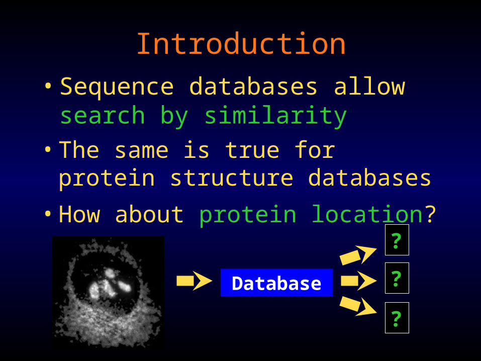
Introduction• Sequence databases allow search by

similarity

Database

?

?

?

• The same is true for protein structure databases

• How about protein location?

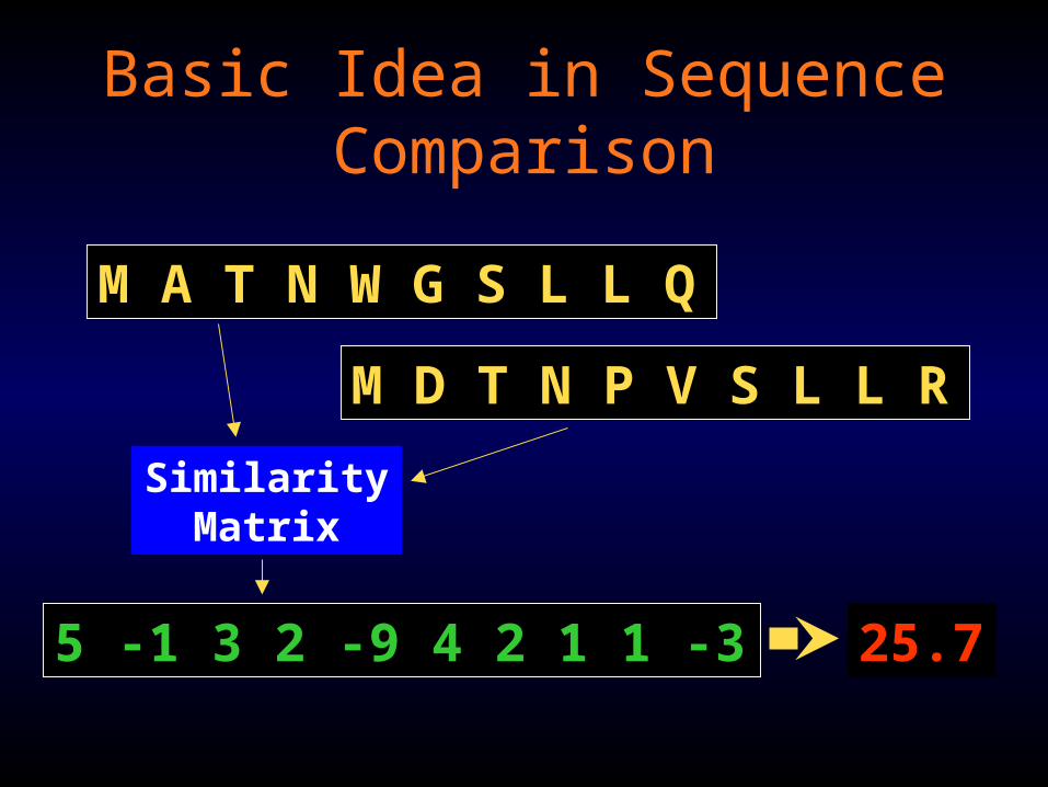
Basic Idea in Sequence Comparison

M A T N W G S L L Q

M D T N P V S L L R

5 -1 3 2 -9 4 2 1 1 -3

Similarity Matrix

25.7

Location Info in Databases

• Unstructured text - most databases

• Standardized keywords - YPD

• Fluorescence microscope images - TRIPLES, YPL.db

• Numerical descriptors needed

7.84 -0.097 24 1 2.3 -31.03 -2

Subcellular Location Features (SLF)

• 49 Zernike Moments• 13 Haralick Texture Features• 22 Morphological Features - derived from

morphological image processing:– Object finding– Edge finding– Convex Hulls

Morphological Features

Area

Distance from COF

Distance from DNA COF

894

89

102

252

23

12

Some Example Features– Number of Objects

– Euler Number

– Average Object Size

– Standard Deviation of Object sizes

– Ratio of the Largest to the Smallest Object Size

– Average Distance of Objects from COF

– Standard Deviation of Object Distances from COF

– Ratio of the Largest to Smallest Object Distance

DNA Features– The average object distance from the COF of the DNA

image– The variance of object distances from the DNA COF– The ratio of the largest to the smallest object to DNA COF

distance– The distance between the protein COF and the DNA COF– The ratio of the area occupied by protein to that occupied

by DNA– The fraction of the protein fluorescence that co-localizes

with DNA

Ten Major Classes of Protein Location

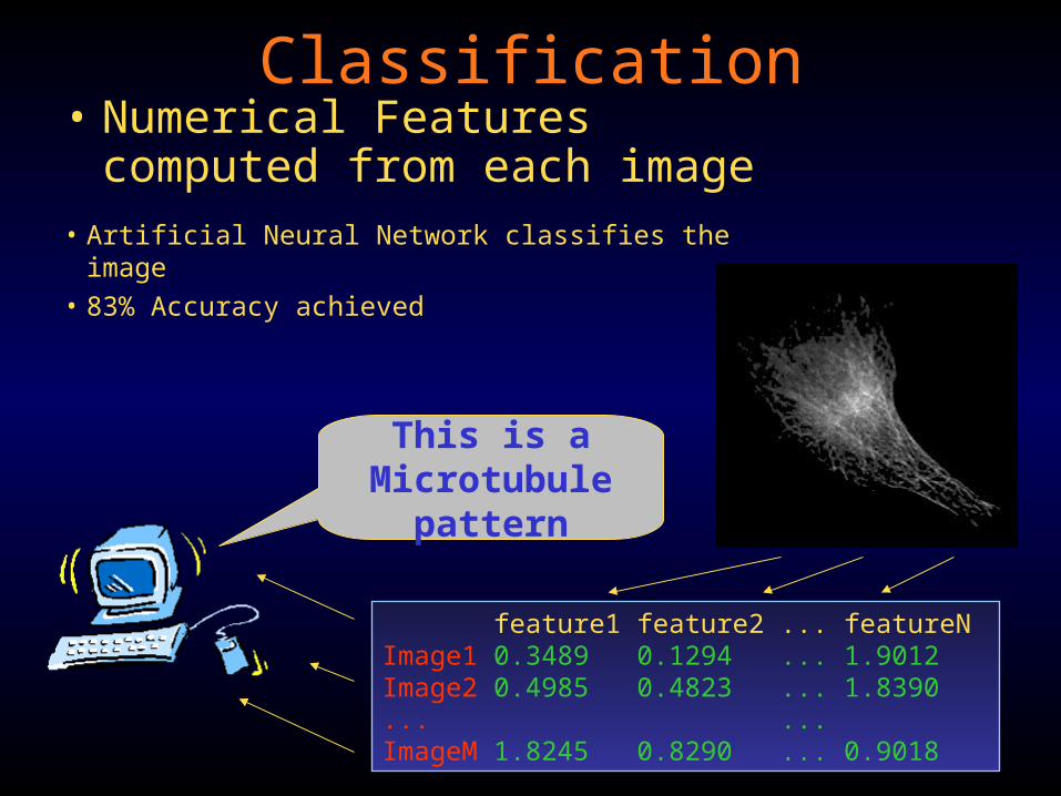
Classification• Numerical Features computed

from each image

This is aMicrotubule

pattern

feature1 feature2 ... featureNImage1 0.3489 0.1294 ... 1.9012Image2 0.4985 0.4823 ... 1.8390... ...ImageM 1.8245 0.8290 ... 0.9018

• Artificial Neural Network classifies the image• 83% Accuracy achieved

Goals

• Implement new 2D features and improve Haralick texture features

• Test performance on mixtures of more than one cell type and more than one microscopy source

• Extend features to 3D

• Develop Object-level classification

• Skeleton Features:– Length of skeleton– Number of branch points– Fraction of object area taken up by skeleton

• Fraction of fluorescence below threshold

New Features (SLF7)

• Based on gray-level co-occurrence

• If image has G gray-levels:– Compute G x G co-occurrence probability

matrix P( i, j)– Compute features by summing and differencing

the matrix

• Features highly dependent on:– Number of gray-levels– Pixel resolution

Haralick Texture Features

Percent Benefit of Texture Features

Baseline accuracy = 86.4%

Solution

• Always down-sample and re-quantize to:– 1.15 um/pixel

– 256 gray-levels

• Resolution-independent robust classification possible

Original Image

256 Gray-levels, 0.23 um/pixel

Down-sampled

256 Gray-levels, 1.15 um/pixel

Classification Results with SLF8

Overall accuracy = 88%

Classification of Images from Mixed Sources

Overall accuracy = 92%

97102Tubul

28981Lyso

23951Golgi

73188DNA

TubulLysoGolgiDNA

Tru

e C

lass

Predicted Class

Extending to 3D• Results for 2-D images can be dependent on

the z-position of the slice

BOTTOM TOP

Extending to 3D

• Features sensitive to 3D distribution will be needed for polarized cells (e.g. epithelial cells)

• Proteins may distribute differently to the basolateral and apical surfaces

Actin (Microfilament)

Tubulin (Microtubule)

Mitochondrial

Endoplasmic Reticulum (ER)

TfR (Endosomal)

LAMP2 (Lysosomal)

Giantin (Golgi)

gpp130 (Golgi)

Nucleolin (Nucleolar)

DNA (Nuclear)

Total-Protein (Cytoplasmic)

Features for 3-D Images• Used a subset of the same Morphological

features as used with 2-D patterns:– Number of Objects– Euler Number– Average Object Size– Standard Deviation of Object sizes– Ratio of the Largest to the Smallest Object Size– Average Distance of Objects from COF– Standard Deviation of Object Distances from COF– Ratio of the Largest to Smallest Object Distance

Separating Components of Distance Features

• Can separate out Horizontal and Vertical components of distance– 2D euclidean for x and y– Signed 1D distance for z

• Some morphological features involve measures of distance– e.g., Average distance of objects from the COF of DNA

Classification with 3D-SLF9 Features

10 classes, Overall accuracy = 91%

Classification with 3D-SLF9 Features

11 classes, Overall accuracy = 91%

11 classes, Overall accuracy = 94%

…with 9 Selected 3D-SLF9 Features

2D Classification with 14 SLF2 Features

11 classes, Overall accuracy = 88%

Set size 9, Overall accuracy = 99.7%

Classification of Sets of 3D Images

Conclusions

• For accurate determination of subcellular location:– High resolution microscopy is essential– 3D images have an advantage over 2D images– SDA can achieve severely sub-optimal results

• Protein Subcellular Location Patterns can be represented as Numerical Vectors

• Can be computed from either 2D or 3D images

• Features are robust to different microscopy methods or cell types

Conclusions

Conclusions

Feature Extractor

38.1

• Quantitative comparison of location is possible

7.84 -0.097 24 1 2.3 -31.03 -2

2.19 +0.271 98 8 0.9 -11.21 0

Roques and Murphy (2002)

• Protein databases can be searched by similarity of location

Database

crp21

froX

CAP-9

Conclusions

• Automated interpretation of location patterns is possible:

– Automated classification of location patterns (Boland and Murphy, 2001; Murphy et al. 2001; Velliste and Murphy, 2002)

– Automated choice of representative images (Markey et al. 1999)

– Rigorous statistical comparison of imaging experiments (Roques and Murphy, 2002)

– Building a “family tree” of protein location

Conclusions

Acknowledgements

• Robert F. Murphy - for being a great thesis advisor

• Michael V. Boland - founding work on 2D Subcellular Location Features

• Simon Watkins and the staff at the Center for Biologic Imaging at UPitt - providing the facilities for and assisting with microscopy

• Aaron C. Rising - help with collecting 3D images

• Gregory Porreca - improving Haralick features and classifying mixed image sets