impact of brine-induced stratiﬁcation on the glacial ... · impact of brine-induced...

Clim. Past, 6, 575–589, 2010www.clim-past.net/6/575/2010/doi:10.5194/cp-6-575-2010© Author(s) 2010. CC Attribution 3.0 License.

Climateof the Past

Impact of brine-induced stratification on the glacial carbon cycle

N. Bouttes1, D. Paillard1, and D. M. Roche1,2

1Laboratoire des Sciences du Climat et de l’Environnement, IPSL-CEA-CNRS-UVSQ, UMR 8212, Centre d’Etudes deSaclay, Orme des Merisiers bat. 701, 91191 Gif Sur Yvette, France2Faculty of Earth and Life Sciences, Section Climate Change and Landscape dynamics, Vrije Universiteit Amsterdam,De Boelelaan, 1085, 1081 HV Amsterdam, The Netherlands

Received: 26 March 2010 – Published in Clim. Past Discuss.: 26 April 2010Revised: 23 August 2010 – Accepted: 31 August 2010 – Published: 15 September 2010

Abstract. During the cold period of the Last Glacial Maxi-mum (LGM, about 21 000 years ago) atmospheric CO2 wasaround 190 ppm, much lower than the pre-industrial con-centration of 280 ppm. The causes of this substantial dropremain partially unresolved, despite intense research. Un-derstanding the origin of reduced atmospheric CO2 duringglacial times is crucial to comprehend the evolution of thedifferent carbon reservoirs within the Earth system (atmo-sphere, terrestrial biosphere and ocean). In this context, theocean is believed to play a major role as it can store largeamounts of carbon, especially in the abyss, which is a car-bon reservoir that is thought to have expanded during glacialtimes. To create this larger reservoir, one possible mecha-nism is to produce very dense glacial waters, thereby strati-fying the deep ocean and reducing the carbon exchange be-tween the deep and upper ocean. The existence of such verydense waters has been inferred in the LGM deep Atlanticfrom sediment pore water salinity andδ18O inferred temper-ature. Based on these observations, we study the impact ofa brine mechanism on the glacial carbon cycle. This mech-anism relies on the formation and rapid sinking of brines,very salty water released during sea ice formation, whichbrings salty dense water down to the bottom of the ocean.It provides two major features: a direct link from the sur-face to the deep ocean along with an efficient way of set-ting a strong stratification. We show with the CLIMBER-2carbon-climate model that such a brine mechanism can ac-count for a significant decrease in atmospheric CO2 and con-tribute to the glacial-interglacial change. This mechanismcan be amplified by low vertical diffusion resulting fromthe brine-induced stratification. The modeled glacial dis-

Correspondence to:N. Bouttes([email protected])

tribution of oceanicδ13C as well as the deep ocean salinityare substantially improved and better agree with reconstruc-tions from sediment cores, suggesting that such a mechanismcould have played an important role during glacial times.

1 Introduction

Proxy data suggest that the climate of the Last Glacial Max-imum (LGM, about 21 000 years ago) was very cold (−2to −6◦C in the Southern Ocean surface (MARGO ProjectMembers, 2009)) with huge Northern Hemisphere ice sheets(Peltier, 2004). The associated carbon cycle was character-ized by low atmospheric CO2 concentrations of∼190 ppm(Monnin et al., 2001) and very negative deep oceanδ13C.The latter is based on the stable carbon isotopic composition(δ13C) of benthic foraminifera which is assumed to reflecttheδ13C of total dissolved inorganic carbon (DIC) in bottomwaters.

The Atlanticδ13C reached low values down to−0.8‰ inthe deep ocean participating in a higher upper to deep oceanicgradient (Duplessy et al., 1988; Curry and Oppo, 2005;Kohler and Bintanja, 2008). The mean upper (−2000 m to0 m) to deep (−5000 m to−3000 m) gradient in the Atlantic,(noted1δ13Catl), was about 1.2‰ in the Atlantic, comparedto only 0.4‰ during the pre-industrial.

LGM climate can be explained by the extended icesheets in connection with a different orbital configuration(Berger, 1978) and lower CO2 (Jahn et al., 2005). To ex-plain the crucial question of the low glacial CO2 numer-ous hypotheses have been proposed. Some of them im-ply changes of physical mechanisms such as modificationsof sea ice coverage (Stephens and Keeling, 2000) or winds(Toggweiler et al., 2006). Many have focused on enhancing

Published by Copernicus Publications on behalf of the European Geosciences Union.

http://creativecommons.org/licenses/by/3.0/

576 N. Bouttes et al.: Brine-induced stratification

or making more efficient the marine biology, for examplethrough higher C/P ratio (Broecker and Peng, 1982), ironfertilization (Martin, 1990), a shift of dominant planktonspecies (Archer and Maier-Reimer, 1994), larger nutrientsavailability (Matsumoto et al., 2002), or modified rain ratio(Brovkin et al., 2007). Other studies have involved coral reeffluctuations (Berger, 1982; Opdyke and Walker, 1992), oroceanic chemistry with carbonate compensation (Broeckerand Peng, 1987). But most only have a small impact on CO2compared to the glacial-interglacial change, or would requireunrealistic modifications to become dominant (Archer et al.,2000, 2003; Kohfeld et al., 2005; Menviel et al., 2008b).Moreover, it has remained especially difficult to correctlysimulate simultaneously the very negativeδ13C in the deepocean inferred from marine sediment cores, although part ofthe change is due to the glacial reduced terrestrial biospherewhich releases light12C leading to a reduction of the globalmean oceanicδ13C (Kohler et al., 2010). Additionally, thestrong link between Antarctic temperatures and atmosphericCO2 variations (Luthi et al., 2008) suggests that mechanismsclosely tied to Southern Ocean surface processes are likely tobe dominant in controlling atmospheric CO2 variability.

The general consensus is that the ocean is at the core of thesolution regarding LGM CO2. It is the biggest carbon reser-voir active on the short time scale studied (a few thousandyears) and the only one that could increase during glacialtimes, since the other two reservoirs, i.e., the atmosphere(Monnin et al., 2001) and terrestrial biosphere (Bird et al.,1994; Crowley, 1995), were both reduced. Observations in-dicate that the deep glacial ocean was much saltier and colderthan today (Adkins et al., 2002), thus more stratified in theabyss. Such a deep stratification has important impacts onthe ocean’s circulation and carbon cycle, as pointed out byclimate models of different complexities (Toggweiler, 1999;Paillard and Parrenin, 2004; Kohler et al., 2005a; Boutteset al., 2009; Tagliabue et al., 2009). In particular, deepstratification is required to reconcileδ13C (Bouttes et al.,2009; Tagliabue et al., 2009). However, only box modelscould significantly reduce atmospheric CO2 when prescrib-ing a reduced Southern ventilation (Watson and Garabato,2005). With models of higher complexity (Bouttes et al.,2009; Tagliabue et al., 2009) the induced CO2 drop remainedtoo small which highlights the need of another mechanismthat would still maintain the benefits of deep stratification(deep negativeδ13C values) while reducing CO2 more dras-tically.

Here we test the impact of the formation and rapid deepsinking of brines, i.e. very salty waters rejected during sea iceformation, on the glacial carbon cycle. The role of brines hasbeen previously proposed as an explanation for the reducedSouthern ventilation (Paillard and Parrenin, 2004; Kohleret al., 2005a; Watson and Garabato, 2005), but they werenot explicitly simulated. Instead, the proposed effect of re-ducing the ventilation was tested by imposing lower mixingin box models only. Here we directly test this mechanism

with a more complex model which physically includes ad-vection and diffusion in the ocean and thus is able to repro-duce the dynamical effect of brines. Because they are en-riched in salt, these “pockets of water” are very dense. In themodern Antarctic they are generally mixed with fresh waterfrom ice shelf melting (Joughin and Padman, 2003). How-ever, during the glacial periods the sea level progressively fell(down to about 120 m at the Last Glacial Maximum) and thenorthward Antarctic ice sheet extent resulted in a progressivereduction of the shelf slope (Ritz et al., 2001) where mod-ern waters are mixed. Tidal dissipation, which is importantin today’s mixing, would then seriously decrease. Accord-ingly, the brine signal, which is diluted today, would be morepreserved at the LGM. Furthermore, the sea ice formationlocation would also shift northward and closer to the conti-nental shelf break. The preserved brine-dense water, whosevolume was increased because of enhanced sea ice forma-tion, would arrive at the shelf break and then flow quicklydown the slope (helped by thermobaricity and supercriticalflux properties) (Foldvik et al., 2004). This mechanism (re-ferred herein thereafter as the brine mechanism) provides twomajor features: a direct link from the surface to the deepocean and an effective physical way of achieving a strongstratification. In this study we test its impact on the carboncycle and compare the modeled results to atmospheric CO2,oceanicδ13C and salinity data inferred from ice core and ma-rine sediment cores.

2 Methods

2.1 CLIMBER-2 model

The brine mechanism has been implemented and tested inCLIMBER-2, an intermediate complexity climate model(Petoukhov et al., 2000) well suited for the long term sim-ulations we run. Indeed, the simulations are run for 20 000years to ensure the equilibrium of the carbon cycle. More-over we realize an ensemble of about 100 simulations to testthe mechanism, which would be unfeasible with a generalcirculation model (GCM) in a reasonable amount of time.The intermediate complexity model, although simpler than astate of the art OGCM, includes the main known processesand mechanisms and computes the dynamics of the oceaniccirculation contrary to box models. Furthermore, like GCMs,CLIMBER-2 does not exhibit box model sensitivity to high-latitude sea ice or presumably stratification (Archer et al.,2003). Additionally, the model compares favourably with astate of the art OGCM and gives the same response in termsof carbon cycle when the circulation is arbitrarily modified(Tagliabue et al., 2009).

CLIMBER-2 has a coarse resolution of 10◦ in latitude by51◦ in longitude in the atmosphere, and 21 depth levels by2.5◦ latitude in the zonally averaged ocean, which is pre-cise enough to take into account geographical changes, while

Clim. Past, 6, 575–589, 2010 www.clim-past.net/6/575/2010/

N. Bouttes et al.: Brine-induced stratification 577

allowing the model to be fast enough to run the long simu-lations considered. The model is composed of various mod-ules simulating the ocean, the atmosphere, and the continen-tal biosphere dynamics. No sediment model is included, themodel thus does not take into account the carbonate com-pensation mechanism. CLIMBER-2 has already been usedand evaluated in previous studies (Ganopolski et al., 2001a;Brovkin et al., 2002a,b, 2007; Bouttes et al., 2009). As themodel version used explicitly computes the evolution of thecarbon cycle and carbon isotopes (such asδ13C) in everyreservoirs, it allows us to compare the model output withdata from sediment cores. In the glacial simulations threeboundary conditions are simultaneously imposed: the icesheets (Peltier, 2004), the solar insolation (Berger, 1978),and the atmospheric CO2 concentration for the radiative forc-ing (190 ppm, not used in the carbon cycle part of the model)(Monnin et al., 2001). To account for the glacial sea levelfall of about 120 m, salinity and nutrients (NO−

3 and PO2−

4 )mean concentrations are increased by 3.3%.

2.2 Implementation of brines in the CLIMBER-2 model

When sea ice is formed, a flux of ions is released into theocean as sea ice is mostly composed of fresh water (Wakat-suchi and Ono, 1983; Rysgaard et al., 2007, 2009). Be-cause the underlying water is then enriched in salt it becomesdenser and can thus sink and transport salt to deeper waters.The rejection of salt by sea ice formation plays an impor-tant role in the formation of deep water, as it is the case forthe Antarctic Bottom Water (AABW) which has been stud-ied for a few decades (Foster and Carmack, 1976; Whitworthand Nowlin, 1987; Foldvik et al., 2004; Nicholls et al., 2009).The brine mechanism has been mostly observed in details inthe Northern Hemisphere oceans (Haarpaintner et al., 2001;Shcherbina et al., 2003; Skogseth et al., 2004, 2008), wheremeasures are easier than in the Southern Ocean. For in-stance, measures in the Arctic fjords indicate that approxi-mately 78% of the brine-enriched shelf water was releasedout of the fjord in the Norwegian Sea (Haarpaintner et al.,2001), i.e. around 62% of the salt flux rapidly released bysea ice formation (the first rapid salt release is∼82% of thetotal salt flux rejected by sea ice formation). The impact ofthe brine formation on the concentration of other geochem-ical variables, especially dissolved inorganic carbon (DIC)has also been studied and it has been shown that DIC is re-jected together with brine from growing sea ice (Rysgaardet al., 2007, 2009). Besides, numerical studies of this localmechanism show that the topography plays an important rolein the transport of salt (Kikuchi et al., 1999).

Thus although today the brine formation around Antarc-tica does not affect the bottom waters (Toggweiler andSamuels, 1995), the formation and sinking of brines is amechanism that can be observed and studied in some placesof the modern ocean and that strongly depends on local con-ditions. The inferred higher salinity in the glacial Southern

Ocean seems to indicate that enhanced brine formation andsinking could well have taken place around Antarctica duringglacial conditions, which should be tested.

In order to assess the potential impact of the sinking ofbrines on the carbon cycle we need to use a global carbon-climate model. Yet the spatial resolution of such models,even state of the art GCMs, is too large to resolve the brinesink, requesting a parameterization. We thus develop a sim-ple parameterization for this mechanism. The simplicity ofthe scheme used permits a first evaluation of such a mech-anism and allows a separation of the different processes tounderstand the reasons of the changes observed.

The sinking of brines initially depends on the amount ofsalt rejected which is determined by the rate of sea ice for-mation. In CLIMBER-2, sea ice formation is computed by aone layer thermodynamic sea ice model with a simple param-eterization for horizontal ice transport (Brovkin et al., 2007).The sea ice extent is increased in winter in agreement withproxy data (Gersonde et al., 2005) although during summersea ice extent is also increased contrary to the data whichindicate a sea ice covered area similar to the modern one.

During the formation of sea ice, in the standard versionof CLIMBER-2 only the flux of salt (FS) was considered.It is usually a good approximation on the first order, yet therelease of other ions and dissolved gases could be of impor-tance for this study. Hence we have added the same processas the release of salt for the other ions and dissolved gasessimulated in the model (dissolved inorganic carbon (DIC), al-kalinity (ALK), nutrients, dissolved organic carbon, oxygen,DI13C, DI14C). As a first approximation the surface oceaniccell is enriched in these geochemical variables in the sameproportion as salt as it has been observed to be not very dif-ferent on the first order (Rysgaard et al., 2007, 2009). Theflux (FX) of any geochemical variableX rejected during seaice formation to the surface ocean is then:

FX =FS

Ssurface·Xsurface (1)

With FS the flux of salt,Ssurface the surface salinity, andXsurface the surface concentration of any geochemical vari-able.

This process is active in all simulations, though it has asmall impact on the standard pre-industrial and LGM simu-lations (atmospheric CO2 is changed by less than 5 ppm).

In the standard version of CLIMBER-2 when sea ice isformed all the salt is released in the corresponding surfaceoceanic cell, which is relatively large according to the coarseresolution of the model and thus dilutes the brine signal.In the brine simulations, a fixed fraction (frac) of this saltflux (and of the other ions flux) will form the sinking brines(Fig. 1a). This fractionfrac can be set to 0 when none ofthe salt sinks to the bottom of the ocean (standard version ofthe model) and 1 when all the salt is used in the brine mech-anism. The very salty (thus dense) brine water sinks to thebottom of the ocean where it modifies the concentration of

www.clim-past.net/6/575/2010/ Clim. Past, 6, 575–589, 2010


ions flux

sea ice formation

(1-frac) x FX

sea ice melting

fresh water flux

surface

bottom

frac x FX

brines

salty dense water

a

b

Fig. 1. (a) Brine sinking mechanism scheme and (b) Potential density difference between thedeep Atlantic ocean (between -5000 m and -3000 m) and the upper Atlantic ocean (between-2000 m and 0 m) as a function of the fraction of salt released by sea ice formation used forthe brine mechanism (fraction of salt frac, 0≤ frac≤ 1). (a) When sea ice is formed salt andother modeled ions (and dissolved gases), such as dissolved inorganic matter (DIC), alkalinity(ALK), dissolved organic carbon (DOC), nutrients, oxygen, DI13C and DI14C are released intothe surface ocean beneath as a flux (FX which is the flux of variable X). A fraction of this flux(frac×FX ) is dedicated to the brine sinking mechanism and is directly transported to the deepocean instead of being diluted in the surface cell as the rest of the flux ((1−frac)×FX ). Thismechanism both creates a link from the surface to the deep ocean and sets an efficient deepocean stratification as the vertical density gradient increases (b).

25

Fig. 1. (a)Brine sinking mechanism scheme and(b) Potential density difference between the deep Atlantic ocean (between−5000 m and−3000 m) and the upper Atlantic ocean (between−2000 m and 0 m) as a function of the fraction of salt released by sea ice formation used forthe brine mechanism (fraction of saltfrac, 0≤ frac≤ 1). (a) When sea ice is formed salt and other modeled ions (and dissolved gases), suchas dissolved inorganic matter (DIC), alkalinity (ALK), dissolved organic carbon (DOC), nutrients, oxygen, DI13C and DI14C are releasedinto the surface ocean beneath as a flux (FX which is the flux of variableX). A fraction of this flux (frac·FX) is dedicated to the brine sinkingmechanism and is directly transported to the deep ocean instead of being diluted in the surface cell as the rest of the flux ((1− frac) ·FX).This mechanism both creates a link from the surface to the deep ocean and sets an efficient deep ocean stratification as the vertical densitygradient increases (b).

any geochemical variableX (salinity, DIC, ALK, nutrients,dissolved organic carbon, oxygen, DI13C and DI14C) as fol-lowing:

VbottomdXbottom

dt= frac·FX ·area (2)

With Vbottom the volume of the bottom cell,Xbottom theconcentration ofX at the bottom and area the area of the sur-face cell. At the surface the rest of the ion flux from sea iceformation not sinking with brines ((1− frac) ·FX) is dilutedin the surface cell. The geochemical variables are thus mod-ified as following:

VsurfacedXsurface

dt= (1− frac) ·FX ·area (3)

Even if this brine mechanism is idealized, it reflects theimpact of intense Antarctic sea ice formation during theLGM. As the glacial Antarctic ice sheet extends close to thelimit of the continental shelf, sea ice formation enhanced bythe strong katabatic winds happens close to the continentalslope. The brines formed by the coeval salt rejection canthen rapidly sink along the continental slope down to thedeep ocean. Unlike convection, the brine mechanism directlytransports this fraction of salt and other ions (frac·FX) to thedeep ocean, and thus represents a direct link from the surfaceto the bottom of the ocean. Because of the salt transport to

the deep ocean this mechanism leads to enhanced stratifica-tion of the ocean as the density gradient between the deepand upper ocean increases (Fig. 1b).

We present model results and compare them to the maincarbon data available for the LGM, e.g. atmospheric CO2concentration andδ13C distribution in the ocean, which con-stitute a major constraint with which to validate this mech-anism. We also compare model results to the glacial deepocean salinity and114C.

3 Results and discussion

3.1 Standard simulation

The CLIMBER-2 version used here has a closed carbon cy-cle i.e. the total (fixed) amount of carbon is interactivelydistributed between the three reservoirs (atmosphere, ter-restrial biosphere and ocean) (Brovkin et al., 2002a), andthe model does not include carbonate compensation. Fromthe pre-industrial value of 280 ppm, atmospheric CO2 risesto 296 ppm for the standard glacial simulation (LGM-std,Fig. 2a). This CO2 rise is due to the prevailing effect ofincreased ocean salinity and terrestrial vegetation decline(of approximately 700 GtC) which increase CO2, despiteincreased nutrient concentration (linked to sea level drop)and colder sea surface temperatures which decrease CO2.This modeled 16 ppm increase adds to the observed 90 ppm



0 0.2 0.4 0.6 0.8 1180

200

220

240

260

280

300A

tmosp

heri

c C

O2 (

ppm

)

LGM data

PI dataandmodel

no saltin brines

LGMstd

all saltin brines

more saltin brines

a

0 0.2 0.4 0.6 0.8 10.2

0.4

0.6

0.8

1.0

1.2

1.4

∆δ1

3Catl (

perm

il)

LGM data

PI data

PI model

LGMstd

more saltin brines

b

0 0.2 0.4 0.6 0.8 1fraction of salt (frac)

34.5

35.0

35.5

36.0

36.5

37.0

37.5

38.0

Deep S

outh

ern

salin

ity (

perm

il)

LGM data

LGMstd more salt

in brines

PI dataPI model

c

Fig. 2. (a) Atmospheric CO2 concentration, (b) ∆δ13Catl (mean upper (-2000 m to 0 m) todeep (-5000 m to -3000 m) gradient in the Atlantic) and (c) salinity in the deep Southern ocean(Atlantic sector, 50 degrees South, 3626 m depth) as a function of the fraction of salt releasedby sea ice formation used for the brine mechanism (fraction of salt frac, 0≤ frac≤ 1). frac =0 corresponds to the standard simulations without any brine mechanism (all the salt and ionsare diluted in the surface cell where sea ice is formed). When frac = 1 all the released saltand other ions sink with the brine mechanism down to the abyss. The Last Glacial Maximum(LGM) and Pre-industrial (PI) data are from Monnin et al., 2001; Curry and Oppo, 2005; Kohlerand Bintanja, 2008; Adkins et al., 2002.

26

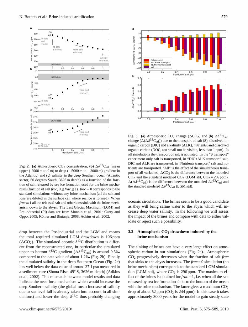
Fig. 2. (a) Atmospheric CO2 concentration,(b) 1δ13Catl (meanupper (-2000 m to 0 m) to deep (−5000 m to−3000 m) gradient inthe Atlantic) and(c) salinity in the deep Southern ocean (Atlanticsector, 50 degrees South, 3626 m depth) as a function of the frac-tion of salt released by sea ice formation used for the brine mecha-nism (fraction of saltfrac, 0≤ frac≤ 1). frac= 0 corresponds to thestandard simulations without any brine mechanism (all the salt andions are diluted in the surface cell where sea ice is formed). Whenfrac= 1 all the released salt and other ions sink with the brine mech-anism down to the abyss. The Last Glacial Maximum (LGM) andPre-industrial (PI) data are from Monnin et al., 2001; Curry andOppo, 2005; Kohler and Bintanja, 2008; Adkins et al., 2002.

drop between the Pre-industrial and the LGM and meansthe total required simulated LGM drawdown is 106 ppm(1CO2). The simulated oceanicδ13C distribution is differ-ent from the reconstructed one, in particular the simulatedupper to bottomδ13C gradient (1δ13Catl) is around 0.5‰compared to the data value of about 1.2‰ (Fig. 2b). Finallythe simulated salinity in the deep Southern Ocean (Fig. 2c)lies well below the data value of around 37.1 psu measured ina sediment core (Shona Rise, 49◦ S, 3626 m depth) (Adkinset al., 2002). This mismatch between model results and dataindicate the need for a mechanism which would increase thedeep Southern salinity (the global mean increase of salinitydue to sea level fall is already taken into account in all sim-ulations) and lower the deepδ13C thus probably changing

0.0 0.2 0.4 0.6 0.8 1.0fraction of salt frac

60

50

40

30

20

10

0

10

Atm

osp

heri

c ∆

CO

2 (

ppm

)

a

S transportDIC+ALK transportNutrients transportAll

0.0 0.2 0.4 0.6 0.8 1.0fraction of salt frac

0.2

0.0

0.2

0.4

0.6

0.8

1.0

∆(∆δ1

3Catl)

(perm

il)

b

Fig. 3. (a) Atmospheric CO2 change (∆CO2) and (b) ∆δ13Catl change (∆(∆δ13Catl)) due tothe transport of salt (S), dissolved inorganic carbon (DIC) and alkalinity (ALK), nutrients, anddissolved organic carbon (DOC, too small too be visible, less than 1 ppm). In all simulationsthe transport of salt is activated. In the “S transport” experiment only salt is transported, in“DIC+ALK transport” salt, DIC and ALK are transported, in “Nutrients transport” salt and nutri-ents are transported. “All” is the effect of the simultaneous transport of all variables. ∆CO2 isthe difference between the modeled CO2 and the standard modeled CO2 (LGM std, CO2 =296ppm). ∆(∆δ13Catl) is the difference between the modeled ∆δ13Catl and the standard modeled∆δ13Catl (LGM std).

27

Fig. 3. (a) Atmospheric CO2 change (1CO2) and (b) 1δ13Catlchange (1(1δ13Catl)) due to the transport of salt (S), dissolved in-organic carbon (DIC) and alkalinity (ALK), nutrients, and dissolvedorganic carbon (DOC, too small too be visible, less than 1 ppm). Inall simulations the transport of salt is activated. In the “S transport”experiment only salt is transported, in “DIC+ALK transport” salt,DIC and ALK are transported, in “Nutrients transport” salt and nu-trients are transported. “All” is the effect of the simultaneous trans-port of all variables.1CO2 is the difference between the modeledCO2 and the standard modeled CO2 (LGM std, CO2 = 296 ppm).1(1δ13Catl) is the difference between the modeled1δ13Catl andthe standard modeled1δ13Catl (LGM std).

oceanic circulation. The brines seem to be a good candidateas they will bring saline water to the abyss which will in-crease deep water salinity. In the following we will assessthe impact of the brines and compare with data to either val-idate or reject such a possibility.

3.2 Atmospheric CO2 drawdown induced by thebrine mechanism

The sinking of brines can have a very large effect on atmo-spheric carbon in our simulations (Fig. 2a). AtmosphericCO2 progressively decreases when the fraction of saltfracthat sinks to the abyss increases. Thefrac= 0 simulation (nobrine mechanism) corresponds to the standard LGM simula-tion (LGM-std), where CO2 is 296 ppm. The maximum ef-fect of the brines is obtained forfrac= 1, i.e. when all the saltreleased by sea ice formation sinks to the bottom of the oceanwith the brine mechanism. The latter gives a maximum CO2drop of about 52 ppm (CO2 is 244 ppm). In this case it takesapproximately 3000 years for the model to gain steady state



-60 -30 0 30 60

4000

3000

2000

1000

0

depth

(m

)PI

a

-60 -30 0 30 60

4000

3000

2000

1000

0LGM, frac=0

b

-60 -30 0 30 60latitude (degree)

4000

3000

2000

1000

0

depth

(m

)

LGM, frac=0.5

c


4000

3000

2000

1000

0LGM, frac=1

d

8

4

0

4

8

12

16

20

24

Fig. 4. Simulated meridional overturning stream function (Sv) in the Atlantic for (a) the Pre-industrial (PI) simulation, (b) the standard LGM simulation (LGM-std) with frac=0 (no impact ofbrines), (c) the LGM simulation with frac=0.5 (medium impact of brines), (d) the LGM simula-tion with frac=1 (maximum impact of brines).

28

Fig. 4. Simulated meridional overturning stream function (Sv) in the Atlantic for(a) the Pre-industrial (PI) simulation,(b) the standard LGMsimulation (LGM-std) withfrac= 0 (no impact of brines),(c) the LGM simulation withfrac= 0.5 (medium impact of brines),(d) the LGMsimulation withfrac= 1 (maximum impact of brines).

again after the onset of the sinking of brines, as the oceancirculation has to adapt to the induced change of density dis-tribution (Fig. 1b).

To understand the reasons of the atmospheric CO2 draw-down, we first assess which variable transport is a major con-tributor to these changes (Fig. 3a). We explore the impact ofthe sinking of salt alone, then we add either dissolved inor-ganic carbon (DIC) and alkalinity (ALK), nutrients (phos-phate and nitrate) or dissolved organic carbon (DOC). Thetransport of salt is activated in all simulations as it is the ini-tial reason for the sinking of the brines.

First we consider only the transport of salt to the deepocean; the other variables do not sink with the brines. Thesalt sink accounts for the largest part of the CO2 drop (ap-proximately 60% of the CO2 drawdown due to the brinemechanism, Fig. 3a). The increased salinity of the bottomwaters results in higher upper to deep ocean density differ-ence (Fig. 1b). Hence the deep stratification is enhancedand the oceanic circulation modified (Fig. 4). In the standardglacial simulation the atlantic meridional overturning circu-lation is slightly different from the pre-industrial one. Theupper branch is shallower while the lower branch more in-tense and penetrates farther north (Fig. 4a and b). With thesinking of salt the vertical density gradient is higher. Thisleads to a more reduced upper branch while the lower branchexpands upwards (Fig. 4c and d). The ventilation of the lowerbranch is reduced resulting in a decoupling between upper

and deep waters. The carbon enriched Antarctic Bottom Wa-ter (AABW) is less mixed with the surrounding waters andconstitutes a greater volume of water. The trapping of CO2released from the remineralization of organic matter in thedeep ocean is then more efficient. The deep carbon reser-voir has thus expanded thanks to the change of circulationinduced by the salt transport alone.

The transport of dissolved inorganic carbon (DIC) and al-kalinity (ALK) by brines also plays a role as it further de-creases atmospheric CO2 (Fig. 3). The direct transport ofDIC and ALK to the abyss helps building an increased deepoceanic carbon reservoir as carbon is brought to the deepocean but can not escape because of the stratification set bythe increased density. In these sensitivity experiments, salt,DIC and ALK are transported. If only DIC and ALK weretransported, the CO2 change would be much greater, but withthe salt transport the DIC and ALK concentrations in the sur-face are already depleted so that the effect of transportingDIC and ALK is not as effective.

The transport of nutrients has an opposite effect, as theirtransport to the abyss decreases their surface concentrationsand thus the biological activity (Fig. 3). The biological pumpbeing less efficient, less atmospheric CO2 is taken up by theocean. Yet this effect is smaller than the two previous ones.Additionaly the transport of DOC is negligible compared tothe other mechanisms (less than 1 ppm).



Now that we have seen that the salt sink is the main driverof the CO2 drop and that the DIC and ALK transport can alsoplay a role, we investigate how they impact the atmosphericCO2. Because of the direct effect of the salt sink (transportfrom the surface to the bottom) and indirect effect (changeof oceanic circulation because of the stratification) the dis-tribution of salinity, DIC and ALK in the ocean is modified(especially the repartition between surface and deep waters).The changed surface concentrations modify the oceanic dis-solved CO2 which ultimately drives atmospheric CO2.

Because of the salt transport by brines, salinity is increasedin the deep ocean (Fig. 2c) and decreased in the surface. Asthe solubility of CO2 increases when salinity decreases itresults in an atmospheric CO2 drawdown. To quantify thisimpact we have run the geochemical module of CLIMBER-2 alone forced by the standard distribution of all variables(from the LGM-std simulation without brines) except salin-ity. For the latter we prescribe the distribution obtained inthe simulation with brines forfrac= 0 to 1. This allows usto get the CO2 change only due to the salinity distributionchange. It appears that the modification of the salinity dis-tribution generally accounts for around 1/4 to a 1/3rd of thetotal CO2 decrease (Fig. 5).

Similarly, DIC and ALK are increased in the deep oceanand decreased in the surface (Fig. 6), both because of thesalt transport induced stratification (we have seen that this isthe main process) and the direct transport of DIC and ALKby brines. To assess the impact of the change of DIC andALK distribution we realize the same test as for salinity.With the geochemical module of CLIMBER-2 we evaluatethe impact of the change of distribution of DIC and ALKalone forfrac= 0 to 1. It shows that the DIC and ALK dis-tribution modification can generally explain between 1/2 and2/3rd of the oceanicpCO2 decrease (Fig. 5). Indeed, as thebrines sink and make the deep ocean saltier, increased verti-cal stratification results. Southern convection (formation ofAntarctic Bottom Water, AABW) is greatly reduced and verylittle exchange exists from the deep ocean to the surface, cre-ating a deep isolated water mass that is enriched in DIC andALK (while the surface is depleted, Fig. 6). With respectto oceanicpCO2, DIC and ALK changes have opposite ef-fects (reduced surface DIC decreasespCO2, reduced ALKincreasespCO2), but the DIC change prevails and results ina net oceanicpCO2 decrease.

3.3 Impact of brines on oceanicδ13C

δ13C is usually used to track oceanic circulation, since theirchanges reflect the changes in ventilation of the different wa-ter masses (Duplessy et al., 1988; Curry and Oppo, 2005;Kohler and Bintanja, 2008). In the brine simulations, themodeled1δ13Catl in the Atlantic Ocean is increased whenthe fraction of saltfrac increases (Fig. 2b), which improvesthe results compared to proxy data. Several mechanisms canaffect 1δ13Catl, as biology and circulation both impact the

0.1 0.2 0.3 0.4 0.5 0.6 0.7 0.8 0.9 1.0fraction of salt frac

0

10

20

30

40

50

pC

O2 d

ecr

ease

(ppm

)

All changesS changes onlyDIC+ALK changes only

Fig. 5. Mean global ocean surface pCO2 decrease due to the brine mechanism as a functionof the fraction of salt rejected by sea ice formation used for the brine mechanism (fraction ofsalt frac, 0≤ frac≤ 1). The pCO2 is calculated from the chemical formulas of the surfaceocean where the geochemical fields (salinity, temperature, DIC and ALK) are imposed andtaken from the simulations with CLIMBER-2. In the pCO2 calculations (except “All changes”)all the geochemical fields are from the standard LGM run (LGM-std, frac=0) except for onevariable. Hence the “S changes only” (red) is the pCO2 change due to the contribution of themodification in the salinity (S) distribution only (the distribution of the other variables is the onefrom the standard simulation). Similarly, the “DIC + ALK changes only” (orange) corresponds tothe contribution of the modification of dissolved inorganic carbon (DIC) and alkalinity (ALK) only.However, “All Changes” (purple) corresponds to the decrease due to the change of distributionof all oceanic variables.

29

Fig. 5. Mean global ocean surfacepCO2 decrease due to the brinemechanism as a function of the fraction of salt rejected by seaice formation used for the brine mechanism (fraction of saltfrac,0≤ frac≤ 1). ThepCO2 is calculated from the chemical formulasof the surface ocean where the geochemical fields (salinity, temper-ature, DIC and ALK) are imposed and taken from the simulationswith CLIMBER-2. In thepCO2 calculations (except “All changes”)all the geochemical fields are from the standard LGM run (LGM-std, frac= 0) except for one variable. Hence the “S changes only”(red) is thepCO2 change due to the contribution of the modificationin the salinity (S) distribution only (the distribution of the other vari-ables is the one from the standard simulation). Similarly, the “DIC+ ALK changes only” (orange) corresponds to the contribution ofthe modification of dissolved inorganic carbon (DIC) and alkalinity(ALK) only. However, “All Changes” (purple) corresponds to thedecrease due to the change of distribution of all oceanic variables.

distribution of δ13C. Indeed, the vertical gradient ofδ13Cis primarily due the biological activity which preferentiallyincorporates12C during photosynthesis. This tends to de-plete the upper waters of12C and hence increaseδ13C. Onthe opposite, when organic matter is remineralized deeper inthe ocean it releases12C thus decreases the deepδ13C. Thisprocess is then modulated by the oceanic circulation whichtransports and mixes water masses with differentδ13C sig-natures and thus modifies theδ13C distribution. With thebrine mechanism these two processes are involved as the salttransport alters circulation, the DIC, ALK and DOC trans-port directly modifies the upper and deepδ13C values, andthe nutrients transport impacts the biological activity.

To assess the role of the salt, DIC and ALK, nutrientsand DOC transport on the increase of1δ13Catl we ana-lyze the same simulations as for CO2, when consideringthe transport of each of the variables (Fig. 3b). As forthe CO2 decrease, the salt transport plays an importantrole. The 1δ13Catl increase is explained entirely by thesalt transport. Because of the brine-induced stratificationand resulting modified circulation (Fig. 4) the waters are lessmixed. Hence the effect of the biological pump becomes



-60 -30 0 30 60

4000

3000

2000

1000

0

depth

(m

)

DIC

frac=0

a

-60 -30 0 30 60

4000

3000

2000

1000

0

depth

(m

)

frac=0.5

c


4000

3000

2000

1000

0

depth

(m

)

frac=1

d

-60 -30 0 30 60

4000

3000

2000

1000

0frac=0

ALKb

-60 -30 0 30 60

4000

3000

2000

1000

0frac=0.5

d


4000

3000

2000

1000

0frac=1

f

1900 2000 2100 2200 2300 2400 2500

Fig. 6. (a,c,d) Dissolved inorganic carbon (DIC) (µmol/kg) and (b,d,f) alkalinity (ALK) (µmol/kg)distribution in the Atlantic for (a, b) the standard simulation (LGM-std) with frac=0 (no impact ofbrines), (c, d) frac=0.5 (medium impact of brines), (e, f) frac=1 (maximum impact of brines).

30

Fig. 6. (a), (c), (e) Dissolved inorganic carbon (DIC) (µmol/kg) and(b), (d), (f) alkalinity (ALK) (µmol/kg) distribution in the Atlantic for(a), (b) the standard simulation (LGM-std) withfrac= 0 (no impact of brines), (c), (d)frac= 0.5 (medium impact of brines), (e), (f)frac= 1(maximum impact of brines).

more important compared to the mixing. The biologicalpump increases the verticalδ13C gradient. On the contrarythe mixing lowers this gradient. Because the mixing is lessintense the vertical gradient increases with lower deepδ13Cand higher upperδ13C.

The DIC and ALK transport as well as nutrient transporthave an opposite yet minor effect. The DIC and ALK trans-port brings high surfaceδ13C values down to the bottom andtends to lower the1δ13Catl, but it has only a small impact ofgenerally less than 0.1‰. The transport of nutrients lowersthe surface nutrient concentration which decreases the bio-logical production. As the latter is responsible for the initial1δ13Catl it also lowers1δ13Catl. However this effect is neg-ligible (less than 0.1‰). Finally the effect of DOC transportis too small to be seen.

It appears that the salt transport is clearly the main pro-cess driving the1δ13Catl increase. On the contrary the othervariables have only a small impact and tend to decrease1δ13Catl. The1δ13Catl is thus improved due to the changeof circulation.

3.4 Amplifications by low vertical diffusion

In the previous simulations, only the impact of brines onconvection and advection was taken into account via salin-ity changes. But it is highly probable that such changeswould also reduce vertical diffusion. CLIMBER-2 prescribesvertical diffusion as a fixed vertical profile, whereas in the-ory it depends on the vertical density profile in the ocean.The brine induced stratification would therefore also change



101 102

Kz (10−4 cm2 /s)

5000

4000

3000

2000

1000

0

Depth

(m

) StandardKz0

Kz1Kz2Kz3

Fig. 7. Vertical diffusion coefficient profiles imposed in the simulations. Kz0 is the standardprofile, Kz1, 2 and 3 are the low diffusion profiles used to test the impact of deep low diffusion.

31

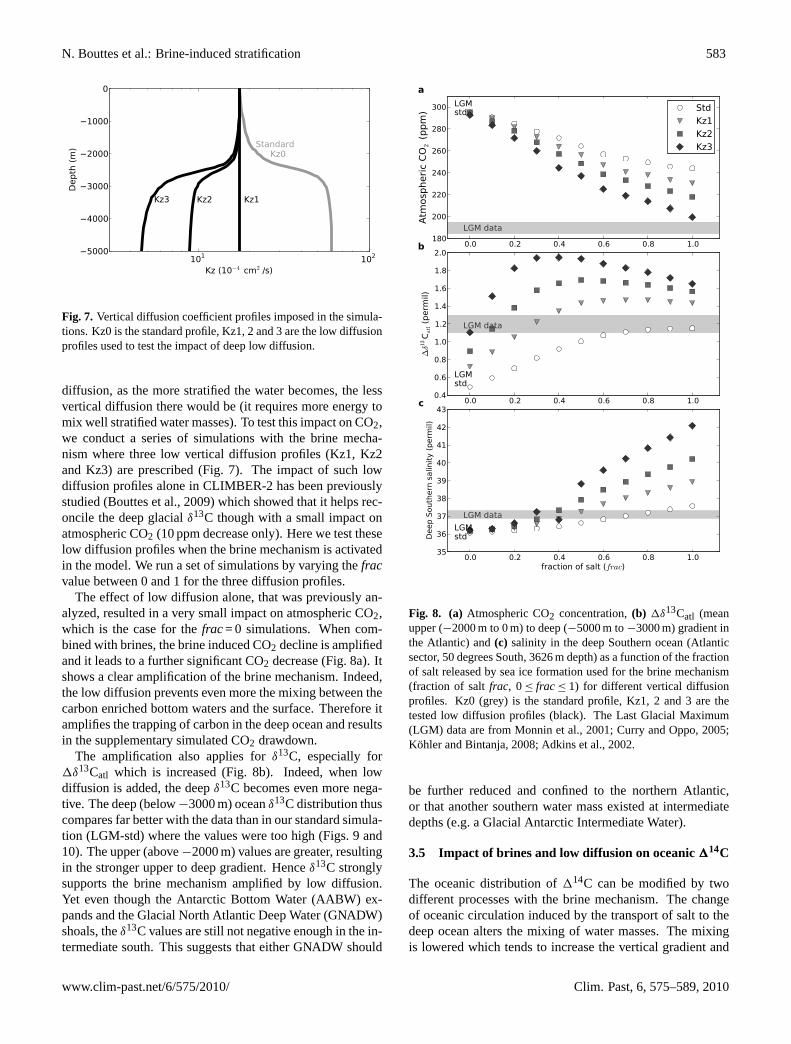
Fig. 7. Vertical diffusion coefficient profiles imposed in the simula-tions. Kz0 is the standard profile, Kz1, 2 and 3 are the low diffusionprofiles used to test the impact of deep low diffusion.

diffusion, as the more stratified the water becomes, the lessvertical diffusion there would be (it requires more energy tomix well stratified water masses). To test this impact on CO2,we conduct a series of simulations with the brine mecha-nism where three low vertical diffusion profiles (Kz1, Kz2and Kz3) are prescribed (Fig. 7). The impact of such lowdiffusion profiles alone in CLIMBER-2 has been previouslystudied (Bouttes et al., 2009) which showed that it helps rec-oncile the deep glacialδ13C though with a small impact onatmospheric CO2 (10 ppm decrease only). Here we test theselow diffusion profiles when the brine mechanism is activatedin the model. We run a set of simulations by varying thefracvalue between 0 and 1 for the three diffusion profiles.

The effect of low diffusion alone, that was previously an-alyzed, resulted in a very small impact on atmospheric CO2,which is the case for thefrac= 0 simulations. When com-bined with brines, the brine induced CO2 decline is amplifiedand it leads to a further significant CO2 decrease (Fig. 8a). Itshows a clear amplification of the brine mechanism. Indeed,the low diffusion prevents even more the mixing between thecarbon enriched bottom waters and the surface. Therefore itamplifies the trapping of carbon in the deep ocean and resultsin the supplementary simulated CO2 drawdown.

The amplification also applies forδ13C, especially for1δ13Catl which is increased (Fig. 8b). Indeed, when lowdiffusion is added, the deepδ13C becomes even more nega-tive. The deep (below−3000 m) oceanδ13C distribution thuscompares far better with the data than in our standard simula-tion (LGM-std) where the values were too high (Figs. 9 and10). The upper (above−2000 m) values are greater, resultingin the stronger upper to deep gradient. Henceδ13C stronglysupports the brine mechanism amplified by low diffusion.Yet even though the Antarctic Bottom Water (AABW) ex-pands and the Glacial North Atlantic Deep Water (GNADW)shoals, theδ13C values are still not negative enough in the in-termediate south. This suggests that either GNADW should

0.0 0.2 0.4 0.6 0.8 1.0180

200

220

240

260

280

300

Atm

osp

heri

c C

O2 (

ppm

)

LGM data

LGMstd

a

StdKz1Kz2Kz3

0.0 0.2 0.4 0.6 0.8 1.00.4

0.6

0.8

1.0

1.2

1.4

1.6

1.8

2.0

∆δ1

3Catl (

perm

il)

LGM data

LGMstd

b

0.0 0.2 0.4 0.6 0.8 1.0fraction of salt (frac)

35

36

37

38

39

40

41

42

43

Deep S

outh

ern

salin

ity (

perm

il)

LGM data

LGMstd

c

Fig. 8. (a) Atmospheric CO2 concentration, (b) ∆δ13Catl (mean upper (-2000 m to 0 m) todeep (-5000 m to -3000 m) gradient in the Atlantic) and (c) salinity in the deep Southern ocean(Atlantic sector, 50 degrees South, 3626 m depth) as a function of the fraction of salt releasedby sea ice formation used for the brine mechanism (fraction of salt frac, 0≤ frac≤ 1) fordifferent vertical diffusion profiles. Kz0 (grey) is the standard profile, Kz1, 2 and 3 are thetested low diffusion profiles (black). The Last Glacial Maximum (LGM) data are from Monnin etal., 2001; Curry and Oppo, 2005; Kohler and Bintanja, 2008; Adkins et al., 2002.32

Fig. 8. (a) Atmospheric CO2 concentration,(b) 1δ13Catl (meanupper (−2000 m to 0 m) to deep (−5000 m to−3000 m) gradient inthe Atlantic) and(c) salinity in the deep Southern ocean (Atlanticsector, 50 degrees South, 3626 m depth) as a function of the fractionof salt released by sea ice formation used for the brine mechanism(fraction of saltfrac, 0≤ frac ≤ 1) for different vertical diffusionprofiles. Kz0 (grey) is the standard profile, Kz1, 2 and 3 are thetested low diffusion profiles (black). The Last Glacial Maximum(LGM) data are from Monnin et al., 2001; Curry and Oppo, 2005;Kohler and Bintanja, 2008; Adkins et al., 2002.

be further reduced and confined to the northern Atlantic,or that another southern water mass existed at intermediatedepths (e.g. a Glacial Antarctic Intermediate Water).

3.5 Impact of brines and low diffusion on oceanic114C

The oceanic distribution of114C can be modified by twodifferent processes with the brine mechanism. The changeof oceanic circulation induced by the transport of salt to thedeep ocean alters the mixing of water masses. The mixingis lowered which tends to increase the vertical gradient and



-60 -30 0 30 60

4000

3000

2000

1000

0

depth

(m

)

DATAinterpolation

a

-60 -30 0 30 60

4000

3000

2000

1000

0

depth

(m

)

frac=0

b

-60 -30 0 30 60

4000

3000

2000

1000

0

depth

(m

)

frac=0.5

d


4000

3000

2000

1000

0

depth

(m

)

frac=1

f

-60 -30 0 30 60

4000

3000

2000

1000

0frac=0, Kz1

c

-60 -30 0 30 60

4000

3000

2000

1000

0frac=0.5, Kz1

e


4000

3000

2000

1000

0frac=1, Kz1

g

1.0 0.6 0.2 0.2 0.6 1.0 1.4

Fig. 9. δ13C (‰) distribution in the Atlantic. The dots represent the LGM data (Curry andOppo, 2005; Kohler and Bintanja, 2008). (a) Interpolation of the data. (b,c,d,e,f,g) Modelledδ13C distribution: (b,d,f) with the standard diffusion profile Kz0 (Figure 7); (c, e, g) with the lowdiffusion profile Kz1 (Figure 7). (b, c) frac=0 (no impact of brines), (d,e) frac=0.5 (mediumimpact of brines), (f,g) frac=1 (maximum impact of brines).

33

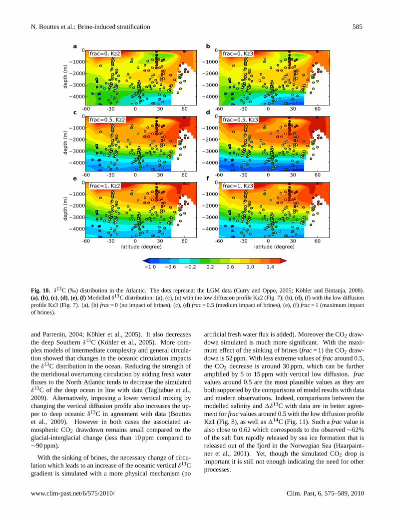
Fig. 9. δ13C (‰) distribution in the Atlantic. The dots represent the LGM data (Curry and Oppo, 2005; Kohler and Bintanja, 2008).(a) Interpolation of the data.(b), (c), (d), (e), (f), (g) Modelled δ13C distribution: (b), (d), (f) with the standard diffusion profile Kz0(Fig. 7); (c), (e), (g) with the low diffusion profile Kz1 (Fig. 7). (b), (c)frac= 0 (no impact of brines), (d), (e)frac= 0.5 (medium impact ofbrines), (f), (g)frac= 1 (maximum impact of brines).

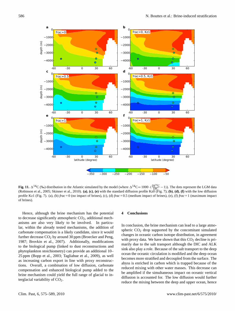
lower δ14C in the deep ocean. On the opposite, the DI14Ctransport during the sinking of brines brings DIC with high14C from the surface to the bottom. It then increases the deep114C values and lower the vertical gradient. The change ofcirculation is the prevailing effect and the deep114C valuesbecome very low (Fig. 11a, c and d). Yet only with the veryextreme and probably unrealisticfrac value (frac=1) can thecirculation capture the increased deep-water ages present inthe data (Robinson et al., 2005; Skinner et al., 2010).

The low diffusion enhances the vertical gradient as thedeep ocean becomes even more isolated. The deep114Cdata values can then be reached with lowerfrac values. Withvery low diffusion profiles (Kz2 and 3, Fig. 12), the deep wa-ter 114C become too low showing that the diffusion shouldbe lowered but not as much.

3.6 Glacial-interglacial carbon cycle changes

Previous studies with simple box models showed that a re-duced Southern ocean vertical mixing rate, which is im-posed in the model, can reduce atmospheric CO2 (Paillard



-60 -30 0 30 60

4000

3000

2000

1000

0

depth

(m

)

frac=0, Kz2a

-60 -30 0 30 60

4000

3000

2000

1000

0

depth

(m

)

frac=0.5, Kz2c


4000

3000

2000

1000

0

depth

(m

)

frac=1, Kz2e

-60 -30 0 30 60

4000

3000

2000

1000

0frac=0, Kz3

b

-60 -30 0 30 60

4000

3000

2000

1000

0frac=0.5, Kz3

d


4000

3000

2000

1000

0frac=1, Kz3

f

1.0 0.6 0.2 0.2 0.6 1.0 1.4

Fig. 10. δ13C (‰) distribution in the Atlantic. The dots represent the LGM data (Curry andOppo, 2005; Kohler and Bintanja, 2008). (a,b,c,d,e,f) Modelled δ13C distribution: (a, c, e) withthe low diffusion profile Kz2 (Figure 7); (b, d, f) with the low diffusion profile Kz3 (Figure 7).(a, b) frac=0 (no impact of brines), (c, d) frac=0.5 (medium impact of brines), (e, f) frac=1(maximum impact of brines).

34

Fig. 10. δ13C (‰) distribution in the Atlantic. The dots represent the LGM data (Curry and Oppo, 2005; Kohler and Bintanja, 2008).(a), (b), (c), (d), (e), (f) Modelledδ13C distribution: (a), (c), (e) with the low diffusion profile Kz2 (Fig. 7); (b), (d), (f) with the low diffusionprofile Kz3 (Fig. 7). (a), (b)frac= 0 (no impact of brines), (c), (d)frac= 0.5 (medium impact of brines), (e), (f)frac= 1 (maximum impactof brines).

and Parrenin, 2004; Kohler et al., 2005). It also decreasesthe deep Southernδ13C (Kohler et al., 2005). More com-plex models of intermediate complexity and general circula-tion showed that changes in the oceanic circulation impactstheδ13C distribution in the ocean. Reducing the strength ofthe meridional overturning circulation by adding fresh waterfluxes to the North Atlantic tends to decrease the simulatedδ13C of the deep ocean in line with data (Tagliabue et al.,2009). Alternatively, imposing a lower vertical mixing bychanging the vertical diffusion profile also increases the up-per to deep oceanicδ13C in agreement with data (Boutteset al., 2009). However in both cases the associated at-mospheric CO2 drawdown remains small compared to theglacial-interglacial change (less than 10 ppm compared to∼90 ppm).

With the sinking of brines, the necessary change of circu-lation which leads to an increase of the oceanic verticalδ13Cgradient is simulated with a more physical mechanism (no

artificial fresh water flux is added). Moreover the CO2 draw-down simulated is much more significant. With the maxi-mum effect of the sinking of brines (frac= 1) the CO2 draw-down is 52 ppm. With less extreme values offrac around 0.5,the CO2 decrease is around 30 ppm, which can be furtheramplified by 5 to 15 ppm with vertical low diffusion.fracvalues around 0.5 are the most plausible values as they areboth supported by the comparisons of model results with dataand modern observations. Indeed, comparisons between themodelled salinity and1δ13C with data are in better agree-ment forfrac values around 0.5 with the low diffusion profileKz1 (Fig. 8), as well as114C (Fig. 11). Such afrac value isalso close to 0.62 which corresponds to the observed∼62%of the salt flux rapidly released by sea ice formation that isreleased out of the fjord in the Norwegian Sea (Haarpaint-ner et al., 2001). Yet, though the simulated CO2 drop isimportant it is still not enough indicating the need for otherprocesses.



-60 -30 0 30 60

4000

3000

2000

1000

0

depth

(m

)

frac=0

a

-60 -30 0 30 60

4000

3000

2000

1000

0

depth

(m

)

frac=0.5

c


4000

3000

2000

1000

0

depth

(m

)

frac=1

e

-60 -30 0 30 60

4000

3000

2000

1000

0frac=0, Kz1

b

-60 -30 0 30 60

4000

3000

2000

1000

0frac=0.5, Kz1

d


4000

3000

2000

1000

0frac=1, Kz1

f

350 300 250 200 150 100 50

Fig. 11. ∆14C (‰) distribution in the Atlantic simulated by the model (where ∆14C= 1000×(DI14C

DIC −1)). The dots represent the LGM data (Robinson et al., 2005; Skinner et al., 2010).(a, c, e) with the standard diffusion profile Kz0 (Figure 7); (b, d, f) with the low diffusion profileKz1 (Figure 7). (a, b) frac=0 (no impact of brines), (c, d) frac=0.5 (medium impact of brines),(e, f) frac=1 (maximum impact of brines).

35

Fig. 11.114C (‰) distribution in the Atlantic simulated by the model (where114C= 1000·(DI14CDIC −1)). The dots represent the LGM data

(Robinson et al., 2005; Skinner et al., 2010).(a), (c), (e) with the standard diffusion profile Kz0 (Fig. 7);(b), (d), (f) with the low diffusionprofile Kz1 (Fig. 7). (a), (b)frac= 0 (no impact of brines), (c), (d)frac= 0.5 (medium impact of brines), (e), (f)frac= 1 (maximum impactof brines).

Hence, although the brine mechanism has the potentialto decrease significantly atmospheric CO2, additional mech-anisms are also very likely to be involved. In particu-lar, within the already tested mechanisms, the addition ofcarbonate compensation is a likely candidate, since it wouldfurther decrease CO2 by around 30 ppm (Broecker and Peng,1987; Brovkin et al., 2007). Additionally, modificationsto the biological pump (linked to dust reconstructions andphytoplankton stoichiometry) can provide an additional 10–25 ppm (Bopp et al., 2003; Tagliabue et al., 2009), as wellas increasing carbon export in line with proxy reconstruc-tions. Overall, a combination of low diffusion, carbonatecompensation and enhanced biological pump added to thebrine mechanism could yield the full range of glacial to in-terglacial variability of CO2.

4 Conclusions

In conclusion, the brine mechanism can lead to a large atmo-spheric CO2 drop supported by the concomitant simulatedchanges in oceanic carbon isotope distribution, in agreementwith proxy data. We have shown that this CO2 decline is pri-marily due to the salt transport although the DIC and ALKsink also play a role. Because of the salt transport to the deepocean the oceanic circulation is modified and the deep oceanbecomes more stratified and decoupled from the surface. Theabyss is enriched in carbon which is trapped because of thereduced mixing with other water masses. This decrease canbe amplified if the simultaneous impact on oceanic verticaldiffusion is accounted for. The low diffusion would furtherreduce the mixing between the deep and upper ocean, hence



-60 -30 0 30 60

4000

3000

2000

1000

0

depth

(m

)frac=0, Kz2

a

-60 -30 0 30 60

4000

3000

2000

1000

0

depth

(m

)

frac=0.5, Kz2c


4000

3000

2000

1000

0

depth

(m

)

frac=1, Kz2e

-60 -30 0 30 60

4000

3000

2000

1000

0frac=0, Kz3

b

-60 -30 0 30 60

4000

3000

2000

1000

0frac=0.5, Kz3

d


4000

3000

2000

1000

0frac=1, Kz3

f

350 300 250 200 150 100 50

Fig. 12. ∆14C (‰) distribution in the Atlantic simulated by the model (where ∆14C= 1000×(DI14C

DIC −1)). The dots represent the LGM data (Robinson et al., 2005; Skinner et al., 2010).(a, c, e) with the low diffusion profile Kz2 (Figure 7); (b, d, f) with the low diffusion profile Kz3(Figure 7). (a, b) frac=0 (no impact of brines), (c, d) frac=0.5 (medium impact of brines), (e, f)frac=1 (maximum impact of brines).

36

Fig. 12. 114C (‰) distribution in the Atlantic simulated by the model (where114C= 1000· (DI14CDIC −1)). The dots represent the LGM

data (Robinson et al., 2005; Skinner et al., 2010).(a), (c), (e) with the low diffusion profile Kz2 (Fig. 7);(b), (d), (f) with the low diffusionprofile Kz3 (Fig. 7). (a), (b)frac= 0 (no impact of brines), (c), (d)frac= 0.5 (medium impact of brines), (e), (f)frac= 1 (maximum impactof brines).

decreasing atmospheric CO2 and increasing the1δ13Catl inline with data. We hypothesize that a combination of the al-ready known carbonate compensation mechanism, iron fer-tilization, brine mechanism and low diffusion would be suf-ficient to reach the glacial value of 190 ppm. The brine mech-anism provides two major features: a physical way of settingthe needed glacial deep ocean stratification and a direct con-nection from surface to deep waters, which is crucial to cre-ate a very large deep ocean carbon reservoir. Beyond the un-derstanding of past climate, this mechanism sheds new lighton ocean dynamics. Brines have a crucial role in the forma-tion of deep water and should therefore be better accountedfor in climate models.

Acknowledgements.We thank Alessandro Tagliabue for commentsand ideas, and Laurent Bopp for discussion. We also thank BillCurry and Peter Kohler for providing theδ13C data and VictorBrovkin for his help on the CLIMBER-2 model. We are greatful toElisabeth Michel for her help with114C, and to two anonymousreviewers and Gerald Ganssen for their comments which helpedimprove this manuscript.

Edited by: G. M. Ganssen

The publication of this article is financed by CNRS-INSU.



References

Adkins, J. F., McIntyre, K., and Schrag, D. P.: The salinity, temper-ature, andδ18O of the glacial deep ocean, Science, 298, 1769–1773, 2002.

Archer, D. and Maier-Reimer, E.: Effect of deep-sea sedimentarycalcite preservation on atmospheric CO2 concentration, Nature,367, 260–263, doi:10.1038/367260a0, 1994.

Archer, D., Winguth, A., Lea, D., and Mahowald, N.: What causedthe glacial/interglacialpCO2 cycles?, Rev. Geophys., 38, 159–189, 2000.

Archer, D. E., Martin, P. A., Milovich, J., Brovkin, V., Plattner,G.-K., and Ashendel, C.: Model sensitivity in the effect ofAntarctic sea ice and stratification on atmosphericpCO2, Paleo-ceanography, 18(1), 1012, doi:10.1029/2002PA000760, 2003.

Berger, A. L.: Long-term variations of daily insolation and Quater-nary climatic changes, J. Atmos. Sci., 35, 2362–2368, 1978.

Berger, W. H.: Increase of carbon dioxide in the atmosphere duringDeglaciation: the coral reef hypothesis, Naturwissenschaften, 69,87–88, 1982.

Bird, M. I., Lloyd, J., and Farquhar, G. D.: Terrestrial carbon stor-age at the LGM, Nature, 371, 566, 1994.

Bopp, L., Kohfeld, K. E., Quere, C. L., and Aumont, O.:Dust impact on marine biota and atmospheric CO2 duringglacial periods, Paleoceanography, 18(2), 1046, doi:10.1029/2002PA000810, 2003.

Bouttes, N., Roche, D. M., and Paillard, D.: Impact of strong deepocean stratification on the carbon cycle, Paleoceanography, 24,PA3203, doi:10.1029/2008PA001707, 2009.

Broecker, W. S. and Peng, T.-H., eds.: Tracers in the Sea, Lamont-Doherty Geological Observatory of Columbia University, Pal-isades, New York, USA, 466–484, 1982.

Broecker, W. S. and Peng, T.-H.: The Role of CaCO3 Compen-sation in the Glacial to Interglacial Atmospheric CO2 Change,Global Biogeochem. Cy., 1(1), 15–29, 1987.

Brovkin, V., Hofmann, M., Bendtsen, J., and Ganopolski, A.:Ocean biology could control atmosphericδ13C during glacial-interglacial cycle, Geochem. Geophys. Geosyst., 3(5), 1027, doi:10.1029/2001GC000270, 2002.

Brovkin, V., Bendtsen, J., Claussen, M., Ganopolski, A., Kubatzki,C., Petoukhov, V., and Andreev, A.: Carbon cycle, vegetation,and climate dynamics in the Holocene: Experiments with theCLIMBER-2 model, Global Biogeochem. Cy., 16(4), 1139, doi:10.1029/2001GB001662, 2002a.

Brovkin, V., Ganopolski, A., Archer, D., and Rahmstorf, S.: Lower-ing of glacial atmospheric CO2 in response to changes in oceaniccirculation and marine biogeochemistry, Paleoceanography, 22,PA4202, doi:10.1029/2006PA001380, 2007.

Crowley, T.: Ice Age Terrestrial Carbon Changes Revisited, GlobalBiogeochem. Cy., 9(3), 377–389, 1995.

Curry, W. B. and Oppo, D. W.: Glacial water mass geometry andthe distribution ofδ13C of 6CO2 in the western Atlantic Ocean,Paleoceanography, 20, PA1017, doi:10.1029/2004PA001021,2005.

Duplessy, J.-C., Shackleton, N., Fairbanks, R., Labeyrie, L., Oppo,D., and Kallel, N.: Deep water source variations during the lastclimatic cycle and their impact on the global deepwater circula-tion, Paleoceanography, 3, 343–360, 1988.

Foldvik, A., Gammelsrød, T., Østerhus, S., Fahrbach, E., Rohardt,G., Schroder, M., Nicholls, K. W., Padman, L., and Woodgate,

R. A.: Ice shelf water overflow and bottom water formation inthe southern Weddell Sea, J. Geophys. Res., 109, C02 015, doi:10.1029/2003JC002008, 2004.

Foster, T. D. and Carmack, E.: Temperature and salinity structurein the Weddell Sea, J. Phys. Oceanogr., 6, 36–44, 1976.

Ganopolski, A., Petoukhov, V., Rahmstorf, S., Brovkin, V.,Claussen, M., Eliseev, A., and Kubatzki, C.: CLIMBER-2: Aclimate system model of intermediate complexity, part II: Modelsensitivity, Clim. Dyn., 17, 735–751, 2001a.

Gersonde, R., Crosta, X., Abelmann, A., et al.: Sea-surface temper-ature and sea ice distribution of the Southern Ocean at the EPI-LOG Last Glacial Maximum – A circum-Antarctic view basedon siliceous microfossil records, Quat. Sci. Rev., 24, 869–896,2005.

Haarpaintner, J., Gascard, J. C., and Haugan, P. M.: Ice productionand brine formation in Storfjorden, Svalbard, J. Geophys. Res,106, 14001–14013, 2001.

Jahn, A., Claussen, M., Ganopolski, A., and Brovkin, V.: Quantify-ing the effect of vegetation dynamics on the climate of the LastGlacial Maximum, Clim. Past, 1, 1–7, doi:10.5194/cp-1-1-2005,2005.

Joughin, I. and Padman, L.: Melting and freezing beneath Filchner-Ronne Ice Shelf, Antarctica, Geophys. Res. Lett., 30, 1477, doi:10.1029/2003GL016941, 2003.

Kikuchi, T., Wakatsuchi, M., and Ikeda, M.: A numerical investiga-tion of the transport process of dense shelf water from a conti-nental shelf to a slope, J. Geophys. Res., 104(C1), 1197–1210,1999.

Kohfeld, K. E., Quere, C. L., Harrison, S. P., and Anderson, R. F.:Role of Marine Biology in Glacial-Interglacial CO2 Cycles, Sci-ence, 308, 74–78, 2005.

Kohler, P. and Bintanja, R.: The carbon cycle during the Mid Pleis-tocene Transition: the Southern Ocean Decoupling Hypothesis,Clim. Past, 4, 311–332, doi:10.5194/cp-4-311-2008, 2008.

Kohler, P., Fischer, H., Munhoven, G., and Zeebe, R. E.: Quanti-tative interpretation of atmospheric carbon records over the lastglacial termination, Global Biogeochem. Cy., 19, GB4020, doi:10.1029/2004GB002345, 2005a.

Kohler, P., Fischer, H., and Schmitt, J.: Atmosphericδ13CO2and its relation topCO2 and deep oceanδ13C during thelate Pleistocene, Paleoceanography, 25, PA1213, doi:10.1029/2008PA001703, 2010.

Luthi, D., Floch, M. L., Bereiter, B., Blunier, T., Barnola, J.-M.,Siegenthaler, U., Raynaud, D., Jouzel, J., Fischer, H., Kawamura,K., and Stocker, T. F.: High-resolution carbon dioxide concentra-tion record 650,000-800,000 years before present, Nature, 453,379–382, doi:10.1038/nature06949, 2008.

MARGO Project Members: Constraints on the magnitude andpatterns of ocean cooling at the Last Glacial Maximum, Nat.Geosci., 2, 127–132, doi:10.1038/ngeo411, 2009.

Martin, J. H.: Glacial-Interglacial CO2 change: the iron hypothesis,Paleoceanography, 5, 1–13, 1990.

Matsumoto, K., Sarmiento, J. L., and Brzezinski, M. A.: Silicicacid leakage from the Southern Ocean: A possible explanationfor glacial atmosphericpCO2, Global Biogeochem. Cy. , 16(3),1031, doi:10.1029/2001GB001442, 2002.

Menviel, L., Timmermann, A., Mouchet, A., and Timm, O.:Meridional reorganizations of marine and terrestrial productiv-ity during Heinrich events, Paleoceanography, 23, PA1203, doi:



10.1029/2007PA001445, 2008b.Monnin, E., Indermuhle, A., Daellenbach, A., Flueckiger, J., Stauf-

fer, B., Stocker, T. F., Raynaud, D., and Barnola, J.-M.: Atmo-spheric CO2 Concentrations over the Last Glacial Termination,Science, 291, 112–114, 2001.

Nicholls, K. W., Østerhus, S., Makinson, K., Gammelsrød, T., andFahrbach, E.: Ice-ocean processes over the continental shelf ofthe southern Weddell Sea, Antarctica: A review, Rev. Geophys.,47, RG3003, doi:10.1029/2007RG000250, 2009.

Opdyke, B. N. and Walker, J. C. G.: Return of the coral reef hy-pothesis: Basin to shelf partitioning of CaCO3 and its effect onatmospheric CO2, Geology, 20, 733–736, 1992.

Paillard, D. and Parrenin, F.: The Antarctic ice sheet and the trig-gering of deglaciations, Earth Planet. Sc. Lett., 227, 263–271,2004.

Peltier, W. R.: Global glacial isostasy and the surface of the ice-age Earth: The ICE-5G (VM2) Model and GRACE, Annu. Rev.Earth Planet. Sci., 32, 111–49, doi:10.1146/annurev.earth.32.082503.144359, 2004.

Petoukhov, V., Ganopolski, A., Eliseev, A., Kubatzki, C., andRahmstorf, S.: CLIMBER-2: A climate system model of inter-mediate complexity, part I: Model description and performancefor present climate, Clim. Dynam., 16, 1–17, 2000.

Ritz, C., Rommelaere, V., and Dumas, C.: Modeling the evolutionof Antarctic ice sheet over the last 420,000 years: Implicationsfor altitude changes in the Vostok region, J. Geophys. Res., 106,31,943–31,964, 2001.

Robinson, L. F., Adkins, J. F., Keigwin, L. D., Southon, J., Fernan-dez, D. P., Wang, S.-L., , and Scheirer, D. S.: Radiocarbon Vari-ability in the Western North Atlantic During the Last Deglacia-tion, Science, 310, 1469–1473, doi:10.1126/science.1114832,2005.

Rysgaard, S., Glud, R. N., Sejr, M. K., Bendtsen, J., and Chris-tensen, P. B.: Inorganic carbon transport during sea ice growthand decay: A carbon pump in polar seas, Geophys. Res., 112,C03 016, doi:10.1029/2006JC003572, 2007.

Rysgaard, S., Bendtsen, J., Pedersen, L. T., Ramløv, H., andGlud, R. N.: Increased CO2 uptake due to sea ice growth anddecay in the Nordic Seas, J. Geophys. Res., 114, 114, doi:10.1029/2008JC005088, 2009.

Shcherbina, A. Y., Talley, L. D., and Rudnick, D. L.: Direct Ob-servations of North Pacific Ventilation: Brine Rejection in theOkhotsk Sea, Science, 302, 1952–1955, doi:10.1126/science.1088692, 2003.

Skinner, L. C., Fallon, S., Waelbroeck, C., Michel, E.,and Barker, S.: Ventilation of the Deep Southern Oceanand Deglacial CO2 Rise, Science, 328(5982), 1147–1151,doi:10.1126/science.1183627, 2010.

Skogseth, R., Haugan, P. M., and Haarpaintner, J.: Ice and brineproduction in Storfjorden from four winters of satellite and insitu observations and modeling, J. Geophys. Res., 109, C10 008,doi:10.1029/2004JC002384, 2004.

Skogseth, R., Smedsrud, L. H., Nilsen, F., and Fer, I.: Observa-tions of hydrography and downflow of brine-enriched shelf wa-ter in the Storfjorden polynya, Svalbard, J. Geophys. Res., 113,C08 049, doi:10.1029/2007JC004452, 2008.

Stephens, B. B. and Keeling, R. F.: The influence of Antarctic seaice on glacial-interglacial CO2 variations, Nature, 404, 171–174,2000.

Tagliabue, A., Bopp, L., Roche, D. M., Bouttes, N., Dutay, J.-C.,Alkama, R., Kageyama, M., Michel, E., and Paillard, D.: Quanti-fying the roles of ocean circulation and biogeochemistry in gov-erning ocean carbon-13 and atmospheric carbon dioxide at thelast glacial maximum, Clim. Past, 5, 695–706, doi:10.5194/cp-5-695-2009, 2009.

Toggweiler, J. and Samuels, B.: Effect of Sea Ice on the Salinityof Antarctic Bottom Waters, J. Phys. Oceanogr., 25, 1980–1997,1995.

Toggweiler, J. R.: Variation of atmospheric CO2 by ventilation ofthe ocean’s deepest water, Paleoceanography, 14(5), 571–588,1999.

Toggweiler, J. R., Russell, J. L., and Carson, S. R.: Midlat-itude westerlies, atmospheric CO2, and climate change dur-ing the ice ages, Paleoceanography, 21, PA2005, doi:10.1029/2005PA001154, 2006.

Wakatsuchi, M. and Ono, N.: Measurements of Salinity and Vol-ume of Brine Excluded From Growing Sea Ice, J. Geophys. Res.,88(C5), 2943–2951, 1983.

Watson, A. J. and Garabato, A. C. N.: The role of Southern Oceanmixing and upwelling in glacial-interglacial atmospheric CO2change, Tellus B, 58(1), 73–87, doi:10.1111/j.1600-0889.2005.00167.x, 2005.

Whitworth, T. and Nowlin, W.: Water Masses and currents of theSouthern Ocean, J. Geophys. Res., 92, 6463–6476, 1987.


impact of brine-induced stratiﬁcation on the glacial ... · impact of brine-induced...

Documents