impact of crisis on eu - welcome -...

1

This project has received funding from the European Union’s Seventh Framework Programmefor research, technological development and demonstration under grant agreement no 266800

FESSUDFINANCIALISATION, ECONOMY, SOCIETY AND SUSTAINABLE

DEVELOPMENT

Working Paper Series

No 150

The impact of the Great Recession on the

European Union countries

Jesus Ferreiro, Catalina Galvez, Carmen Gomez

and Ana Gonzalez

ISSN 2052-8035

2


Title: The impact of the Great Recession on the European Union

countries

Authors: Jesus Ferreiro, Catalina Galvez, Carmen Gomez and Ana Gonzalez

Affiliations of authors: Department of Applied Economics V, University of the Basque

Country UPV/EHU

Abstract: Although the Great Recession has been a global phenomenon affecting most

developed (and emerging) economies, in the case of the European Union (EU), there

are significant differences among EU individual countries and among EU groups of

countries, like euro and non-euro countries regarding the depth and duration of the

crisis. The paper analyses the effects of the economic and financial crisis on a set of

seventeen economic and financial variables, comparing the economic performance of

the EU economies before and after the onset of the crisis. The analysis confirms the

hypotheses, first, of the existence of significant differences on the performance during

the crisis of the EU economies, and, second, that the EU economies most affected by

the crisis have been the euro countries, mainly those that join the euro after 1999. In

this sense, and focusing on the Eurozone, the paper shows a rising divergence in the

macroeconomic performance of euro countries, a divergence process that has been

amplified during the Great Recession.

Key words: Great Recession, economic and financial crisis, Great Recession,

European Union, Eurozone, convergence

Journal of Economic Literature classification: C22, O52, O57, P52

3


Contact details:

Jesus Ferreiro: [email protected]

Catalina Galvez: [email protected]

Carmen Gomez: [email protected]

Ana Gonzalez: [email protected]

Acknowledgments:

The research leading to these results has received funding from the European Union

Seventh Framework Programme (FP7/2007-2013) under grant agreement n° 266800.

Website: www.fessud.eu

4


1. Introduction

Although the Great Recession is a global phenomenon, with roots outside the

European Union (EU), its impact has been deeper and longer lasting in the EU than

elsewhere. Indeed, according to the World Economic Outlook Database (April 2015) of

the International Monetary Fund (IMF), the long-term economic growth forecasts (up

to the year 2020) for the EU are much lower than those of the other regions of the

planet. Thus, in 2014 the real GDP of the European Union and the European Monetary

Union (EMU) were only 4.6 per cent and 2.1 per cent higher respectively than in 2006.

The IMF forecasts that in the year 2020 the real GDP of the EU and the Eurozone will

be 17 and 12 per cent, higher respectively, than in 2006. In contrast, the IMF forecasts

the real GDP of United Kingdom, the United States of America and Asian emerging and

developing economies will be, respectively, 22, 28 and 169 per cent higher in 2020 than

in 2006.

However, the impact of the Great Recession has not been the same in all the European

countries. The objective of this paper is to analyze the different effects of the economic

and financial crisis among the European Union Member States, focusing on the

behavior of a number of real and financial variables since the year 2003 to evaluate the

impact of the crisis.

In this sense, the paper is structured in two different but complimentary sections. In

the first section we will analyze the impact of the individual countries that form the

European Union. In these two sections, our objective is to know the countries that have

been more seriously affected by the crisis and to detect whether the membership to

the Eurozone has led to a significantly different impact regarding non-euro EU

countries. In the second section, our attention will be focused on the performance of

the Euro area, with objective of analyzing whether the crisis has led to a coherence of

the Eurozone. Final section summarizes and concludes.

5


2. The impact of financial and economic crisis on the European Union economies

The objective of this section is to analyze the different effects of the economic and

financial crisis among the European Union Member States, focusing on the behavior

of a number of real and financial variables between the years 2003 and 2013 to evaluate

the impact of the crisis. Since we have used data until 2013, we have excluded Croatia

from the EU countries because it joined the EU in this year. Thus, we will analyze the

performance of seventeen economic variables grouped into seven categories:

1. Economic activity: real GDP growth rate, GDP per capita growth rate, potential GDP

growth rate, output gap

2. Labour market: employment growth rate, unemployment rate, real wages growth

rate, real unit labour costs growth rate

3. Income distribution: adjusted wage share, GINI coefficient

4. Inflation: inflation rate (CPI)

5. Balance of payments: balance on current account

6. Public finances: public budget balance, public debt

7. Financial balance sheets of total economy: financial assets, financial liabilities, net

financial assets

The existence of significantly different impacts of the Great Recession on the European

economies questions the sustainability of the current institutional setting of the

European Union and the Eurozone (Benczes and Szent-Ivanyi 2015). Many studies

argue that the increasing heterogeneity in economic performance in the EU as a whole

and the eurozone countries in particular is the direct consequence of the incorporation

of economies with differing structures to those in the pre-existing member states

(Arestis and Sawyer 2012; Bitzenis, Karagiannis, and Marangos 2015; Carrasco and

Peinado 2015; Gibson, Palivos and Tavlos 2014; Mendonça 2014; Perraton 2011;

Onaran 2011). This higher heterogeneity increases the possibility of asymmetric

6


shocks, and, simultaneously, reduces the effectiveness of single and common rules

for macroeconomic policies (Dodig and Herr 2015).

In this section we will analyze the behavior of the former economic variables for each

of the countries belonging to the European Union (EU-27). Given that our objective is

to analyze the impact of the Great Recession on the economic performance of the EU

economies, we will analyze the changes registered for the analyzed variables between

the average value of each variable in the period before the crisis (2003-2007) and after

the crisis (2008-2013). For most variables, we will also analyze the variation between

the data recorded in the years 2007 and 2013. This data will help us to evaluate both

the depth and the duration of the crisis.

2.1 Economic activity

Figure 1. Real GDP growth rate (%)

Source: our calculations based on Eurostat

Figure 1 shows the real GDP growth rate recorded before and after the onset of the

crisis in 2007. It is easy to note the deep impact of the crisis. Before the crisis all EU

countries recorded positive GDP growth rates, most of them above 2%. However,

-6-4-202468

1012

Bel

gium

Bul

gari

a

Cze

chR

epub

lic

Den

mar

k

Ger

man

y

Esto

nia

Irel

and

Gre

ece

Spai

n

Fran

ce

Ital

y

Cyp

rus

Latv

ia

Lith

uani

a

Luxe

mbo

urg

Hun

gary

Mal

ta

Net

herl

ands

Aus

tria

Pol

and

Por

tuga

l

Rom

ania

Slov

enia

Slov

akia

Finl

and

Swed

en

Uni

ted

Kin

gdom

2003-2007 2008-2013

7


between 2008 and 2013, the average annual GDP growth rate has been negative in 13

EU countries, and in eight countries (Ireland, Greece, Spain, Italy, Latvia, Portugal and

Slovenia) this average GDP growth rate has been below -1%. In this period only four

countries (Malta, Poland, Romania and Sweden) have registered average annual

economic growth rates above 1%

Figure 2. Variation of the real GDP growth rate between 2007 and 2013


An alternative way to evaluate the impact of the crisis is to calculate the difference

between the GDP growth rates in 2007 and 2013. This difference, besides working as a

proxy of the duration of the crisis, also is useful to study the depth of the crisis because

it allows to studying the (partial or total) recovery of the economic growth registered

before the Great Recession. Moreover, by comparing the data of the different

countries, we can evaluate the EU most and least affected by the crisis.

Figure 2 shows that only in one country (Hungary) the economic growth in 2013 was

higher than in 2007. However, this result is explained because the economic crisis

began in Hungary in the year 2007, when the GDP growth rate fell from the 3.9% in

-12

-10

-8

-6

-4

-2

0

2

Cyp

rus

Slov

akia

Slov

enia

Gre

ece

Finl

and

Cze

chR

epub

lic

Lith

uani

a

Latv

ia

Bul

gari

a

Irel

and

Pol

and

Esto

nia

Spai

n

Net

herl

ands

Luxe

mbo

urg

Por

tuga

l

Ital

y

Aus

tria

Ger

man

y

Rom

ania

Bel

gium

Fran

ce

Uni

ted

Kin

gdom

Swed

en

Den

mar

k

Mal

ta

Hun

gary

8


2006 to 0.1%. Therefore, in all the EU countries the GDP growth rate in 2013 is well

below than in 2007. However, this deceleration is not homogenous. It must be

emphasized that the most seriously affected countries are members of the Euro zone,

mainly countries that joined the euro after 1999 (EMU-6). Conversely, it is also relevant

to highlight the (relative) better performance of three economies (United Kingdom,

Sweden and Denmark) that do not belong to the euro area.

The second analyzed variable related to the economic activity is the rate of growth of

potential GDP. As can be seen in the figure 3, all the EU economies recorded before

the crisis positive rates of growth of their potential GDP. The highest rates of growth

took place in Latvia and Lithuania, with average annual growth rates above 6%, and

with other economies like Bulgaria, Estonia and Romania, growing above 5%. Italia

was the country with the worst performance, merely 1%.

Figure 3. Average annual potential GDP growth rate (%)

Source: our calculations based on AMECO

The burst of the crisis led to a generalized collapse in the potential growth in Europe.

Only Poland and Slovakia recorded an average potential GDP growth rate over 3%, with

-2-1012345678

Bel

gium

Bul

gari

a

Cze

chR

epub

lic

Den

mar

k

Ger

man

y

Esto

nia

Irel

and

Gre

ece

Spai

n

Fran

ce

Ital

y

Cyp

rus

Latv

ia

Lith

uani

a

Luxe

mbo

urg

Hun

gary

Mal

ta

Net

herl

ands

Aus

tria

Pol

and

Por

tuga

l

Rom

ania

Slov

enia

Slov

akia

Finl

and

Swed

en

Uni

ted

Kin

gdom

2003-2007 2008-2013

9


Malta and Romania registering a rate hardly over 2%. The worst performance has

taken place in Greece and Italy, which have registered negative rates of growth of the

potential GDP. Ireland and Portugal have recorded a zero growth of their potential

GDP, and in Latvia, Hungary and Finland the average potential GDP growth rate has

been below 0.5%.

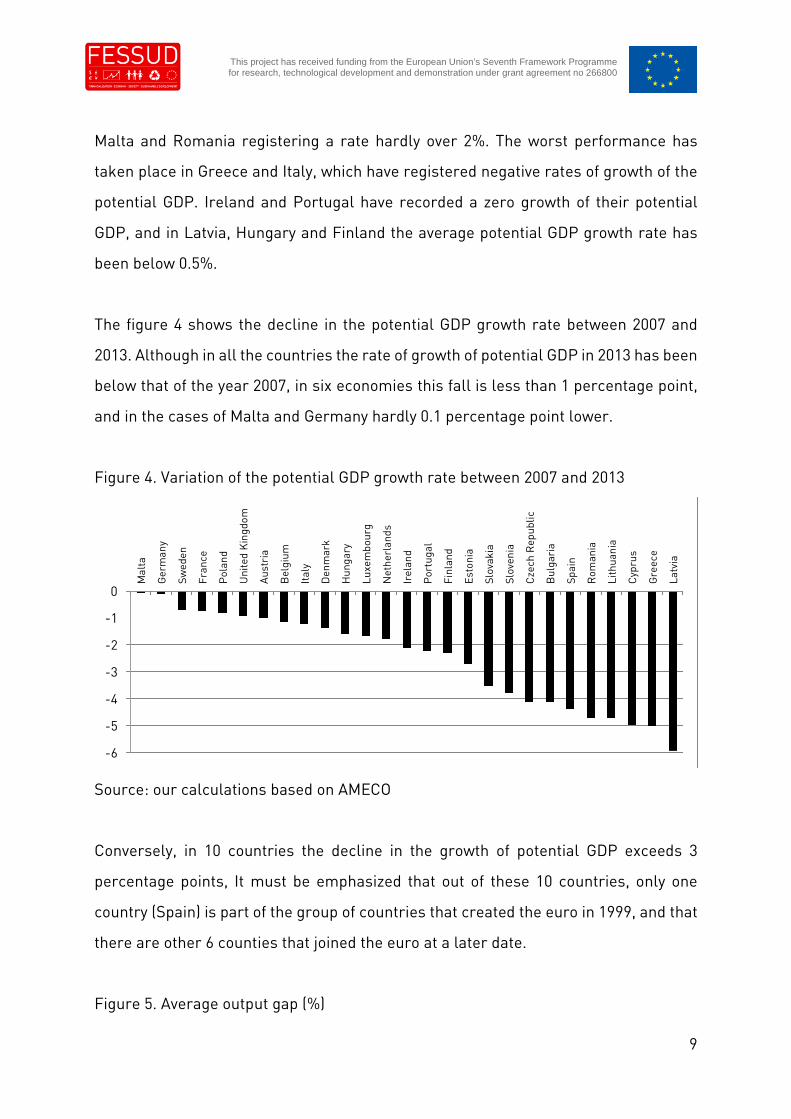
The figure 4 shows the decline in the potential GDP growth rate between 2007 and

2013. Although in all the countries the rate of growth of potential GDP in 2013 has been

below that of the year 2007, in six economies this fall is less than 1 percentage point,

and in the cases of Malta and Germany hardly 0.1 percentage point lower.

Figure 4. Variation of the potential GDP growth rate between 2007 and 2013


Conversely, in 10 countries the decline in the growth of potential GDP exceeds 3

percentage points, It must be emphasized that out of these 10 countries, only one

country (Spain) is part of the group of countries that created the euro in 1999, and that

there are other 6 counties that joined the euro at a later date.

Figure 5. Average output gap (%)

-6

-5

-4

-3

-2

-1

0

Mal

ta

Ger

man

y

Swed

en

Fran

ce

Pol

and

Uni

ted

Kin

gdom

Aus

tria

Bel

gium

Ital

y

Den

mar

k

Hun

gary

Luxe

mbo

urg

Net

herl

ands

Irel

and

Por

tuga

l

Finl

and

Esto

nia

Slov

akia

Slov

enia

Cze

chR

epub

lic

Bul

gari

a

Spai

n

Rom

ania

Lith

uani

a

Cyp

rus

Gre

ece

Latv

ia

10



The output gap can be used to evaluate the business cycle of the EU countries. Looking

of the data of the figure 5, we can see that during the period 2003-2007, all the EU

economies were in an expansion (a positive output gap), with the exceptions of

Germany, Austria Netherlands, Poland and Portugal. The existence of a negative

output gap in these five countries is explained by the bad performance in the first years

of the pre-crisis period. The mirror can be found in Estonia, Latvia, Lithuania and

Romania, whose positive output gaps were above 4%.

On the contrary, during the crisis period (2008-2013), only four countries, Bulgaria,

Cyprus, Slovakia and, mainly, Poland have registered a positive output gap. Measured

by the output gap, the biggest recession has taken place in Greece (-6.5%), followed

by Latvia (-4.4%), Spain (-4.4%), y Portugal (-3.5%). It is remarkable the cases of

Greece, whose output gap reached 14% in 2012 and 2013, and Latvia that in 2009 and

2010 registered an output gap of -11%, when in 2007 its output gap peaked 11.7%.

Figure 6. Variation of the output gap between 2007 and 2013 (percentage points)

-8-6-4-202468

Bel

gium

Bul

gari

a

Cze

chR

epub

lic

Den

mar

k

Ger

man

y

Esto

nia

Irel

and

Gre

ece

Spai

n

Fran

ce

Ital

y

Cyp

rus

Latv

ia

Lith

uani

a

Luxe

mbo

urg

Hun

gary

Mal

ta

Net

herl

ands

Aus

tria

Pol

and

Por

tuga

l

Rom

ania

Slov

enia

Slov

akia

Finl

and

Swed

en

Uni

ted

Kin

gdom

2003-2007 2008-2013

11



Figure 6 shows the variation of the output gap between 2007 and 2013. In six

economies, this variation is above 10 percentage points. But the most remarkable

outcome is that the eight countries that have registered the highest decline in the

output gap belong to the Eurozone, and that only one country, Spain, was one of the

founders of the European Monetary Union in 1999.

2.2 Labour market

The analysis of the impact of the Great Recession on the European labour markets is

carried out on the basis of four variables: the employment growth rate, the

unemployment rate, the rate of growth of real wages, and the rate of growth of real

unit labour costs.

Figure 7. Annual average employment growth rate (%)

-20-18-16-14-12-10

-8-6-4-20

Mal

ta

Ger

man

y

Aus

tria

Bul

gari

a

Bel

gium

Pol

and

Uni

ted

Kin

gdom

Fran

ce

Swed

en

Hun

gary

Net

herl

ands

Ital

y

Luxe

mbo

urg

Irel

and

Por

tuga

l

Rom

ania

Finl

and

Den

mar

k

Cze

chR

epub

lic

Lith

uani

a

Cyp

rus

Spai

n

Latv

ia

Slov

akia

Slov

enia

Esto

nia

Gre

ece

12



The figure 7 shows the average annual total employment growth rate in the EU. If we

focus on the pre-period crisis, the most relevant outcome is that there was a

generalized process of employment creation between 2003 and 2007. Indeed, in these

years only in Portugal and Romania there was a decline in total employment. This

situation changed dramatically after 2008. Between 2008 and 2013 the average annual

employment growth rate has been negative in 16 countries.

As a result, in 17 EU countries the total employment in the year 2013 was below that

existing in 2007 (see figure 8). There are 6 countries where the crisis has destroyed

more than 10 per cent of the employment existing in 2007, and with the only exception

of Bulgaria, all of them belong to the euro area. On the contrary, in 3 economies, there

has been an employment creation process exceeding the figure of 5 per cent.

Figure 8. Variation of total employment in the years 2008 to 2013 (percentage of totalemployment registered in 2007)

-5-4-3-2-1012345

Bel

gium

Bul

gari

a

Cze

chR

epub

lic

Den

mar

k

Ger

man

y

Esto

nia

Irel

and

Gre

ece

Spai

n

Fran

ce

Ital

y

Cyp

rus

Latv

ia

Lith

uani

a

Luxe

mbo

urg

Hun

gary

Mal

ta

Net

herl

ands

Aus

tria

Pol

and

Por

tuga

l

Rom

ania

Slov

enia

Slov

akia

Finl

and

Swed

en

Uni

ted

Kin

gdom

2003-2007 2009-2013

13



Figure 9. Average unemployment rate (%)


It could be expected that the impact of the Great Recession on the European labour

markets had led to a generalized and substantial rise in the unemployment rate. But

this outcome has not taken place. As can be seen in figure 9, in 10 economies the

unemployment rate in 2008-2013 has been lower than that existing in 2003-2007:

Belgium, Bulgaria, Czech Republic, Germany, Netherlands, Poland, Portugal,

-30-25-20-15-10

-505

101520

Gre

ece

Spai

nLa

tvia

Por

tuga

lIr

elan

dLi

thua

nia

Bul

gari

aSl

oven

iaC

roat

iaEs

toni

aD

enm

ark

Ital

yC

ypru

sFi

nlan

dSl

ovak

iaN

ethe

rlan

dsR

oman

iaC

zech

Rep

ublic

Hun

gary

Fran

ceP

olan

dU

nite

dK

ingd

omB

elgi

umSw

eden

Aus

tria

Ger

man

yM

alta

Luxe

mbo

urg

02468

10121416182022

Bel

gium

Bul

gari

a

Cze

chR

epub

lic

Den

mar

k

Ger

man

y

Esto

nia

Irel

and

Gre

ece

Spai

n

Fran

ce

Ital

y

Cyp

rus

Latv

ia

Lith

uani

a

Luxe

mbo

urg

Hun

gary

Mal

ta

Net

herl

ands

Aus

tria

Pol

and

Por

tuga

l

Rom

ania

Slov

enia

Slov

akia

Finl

and

Swed

en

Uni

ted

Kin

gdom

2003-2007 2008-2013

14


Slovenia, Finland and Sweden. However, in most cases, this result is explained by the

high unemployment rates registered in many cases in the early years of the decade of

the 2000s.

Indeed, the results are different when we observe the change in the unemployment

rate between 2007 and 2013 (see figure 10). In these years, the unemployment rate has

increased with only two exceptions: Netherlands and Germany.

Figure 10. Variation of unemployment rate between 2007 and 2013 (percentage points)


In nine countries the unemployment rate has increased in more than 6 percentage

points, standing out the huge increases registered in Greece and Spain (the two

countries with the highest unemployment rate. Again, it must be emphasized that the

six countries with the highest increase of the unemployment rates belong to the

Eurozone.

When we focus on the real wages growth (figure 11), we can see the huge differences

in the real wages growth during the pre-period crisis. The most striking fact is that,

contrary to what happened in the other EU countries, in Germany and Portugal there

was a decline in real wages, with annual real wages growth rates amounting to -0.7

-4-202468

101214161820

Gre

ece

Spai

n

Latv

ia

Irel

and

Luxe

mbo

urg

Ital

y

Rom

ania

Bul

gari

a

Cyp

rus

Lith

uani

a

Slov

akia

Esto

nia

Den

mar

k

Aus

tria

Finl

and

Mal

ta

Fran

ce

Uni

ted

Kin

gdom

Cze

chR

epub

lic

Hun

gary

Swed

en

Bel

gium

Por

tuga

l

Slov

enia

Pol

and

Net

herl

ands

Ger

man

y

15


and -0.1 per cent, respectively. On the contrary, the highest real wages growth rates

took place in Latvia (12.8%), Lithuania (11.4%), Romania (10%) and Estonia (9,6%).

Indeed, in some of these countries the real wages growth rate peaked 20%, as it is the

case of Latvia (2007) and Romania (2005 and 2008). The lowest increase of real wages

took place in Belgium (0.1%), Austria (0.3%) and Spain and Poland (0.4%).

Figure 11. Average real compensation per employee growth rate (%)


With a few exceptions, the Great recession has led to a moderation in the wage growth,

although the number of countries that registers an average negative growth rate of

real wages is low: Czech Republic (-0.1%), Greece (-2.9%), Cyprus (-1.5%), Lithuania

(-0.7%), Hungary (-2.1%) and the United Kingdom (-1%).

However, previous data hide the different behavior of real wages after the onset of the

crisis. In the years 2008 and 2009, real wages only fell in six countries (Lithuania,

Latvia, Czech Republic, Estonia, Hungary and United Kingdom). In most countries, the

real wages kept on rising at similar rates that those registered before the crisis, with

the exceptions of Bulgaria, Ireland and Spain, whose wage growth was substantially

higher than before the crisis (see figure 12).

-4-202468

101214

Bel

gium

Bul

gari

a

Cze

chR

epub

lic

Den

mar

k

Ger

man

y

Esto

nia

Irel

and

Gre

ece

Spai

n

Fran

ce

Ital

y

Cyp

rus

Latv

ia

Lith

uani

a

Luxe

mbo

urg

Hun

gary

Mal

ta

Net

herl

ands

Aus

tria

Pol

and

Por

tuga

l

Rom

ania

Slov

enia

Slov

akia

Finl

and

Swed

en

Uni

ted

Kin

gdom

2003-2007 2008-2013

16


Figure 12. Average real compensation per employee growth rate since 2008 (%)


As can be seen in figure 12, the highest impact of the crisis on real wages has taken

place since 2010. With a few exceptions, the real wages growth rate has been lower in

2010-2013 than in 2008-2009. In 2010-2013 ten economies have registered a decline in

real wages, standing out the negative average annual real wages growth rates of

countries like Portugal (-1%), Spain (-1.2%), Hungary (-2.2%), Cyprus (-2.5), Romania

(-3%) and Greece (-4.7%).

Despite the increase registered in the real wages before the crisis, real unit labour

costs (ULCs) fell in most EU countries in the years previous to the burst of the crisis.

As figure 13 shows, real ULCs only increased in four countries: Estonia, Ireland,

Lithuania and Latvia. It must be highlighted the cases of Bulgaria, Romania, Germany

and Luxembourg, countries in which their real ULCs were declining at an annual rate

above 1.5 per cent.

Figure 13. Average annual real unit labour costs growth rate (%)

-6-5-4-3-2-10123456789

Bel

gium

Bul

gari

a

Cze

chR

epub

lic

Den

mar

k

Ger

man

y

Esto

nia

Irel

and

Gre

ece

Spai

n

Fran

ce

Ital

y

Cyp

rus

Latv

ia

Lith

uani

a

Luxe

mbo

urg

Hun

gary

Mal

ta

Net

herl

ands

Aus

tria

Pol

and

Por

tuga

l

Rom

ania

Slov

enia

Slov

akia

Finl

and

Swed

en

Uni

ted

Kin

gdom

2008-2009 2010-2013

17



This behavior of real ULCs has changed since the year 2008. Real ULCs have increased

between 2008 and 2013 in sixteen countries. As we can see, the larger declines in the

real ULCs have happened in Romania, Latvia, Greece, Lithuania and Cyprus, countries

where the real ULCs are declining since 2008 at an annual rate exceeding 1 per cent.

Figure 14. Real unit labour costs in the European Union (2002=100)

-3.0-2.5-2.0-1.5-1.0-0.50.00.51.01.52.02.53.03.5

Bel

gium

Bul

gari

a

Cze

chR

epub

lic

Den

mar

k

Ger

man

y

Esto

nia

Irel

and

Gre

ece

Spai

n

Fran

ce

Ital

y

Cyp

rus

Latv

ia

Lith

uani

a

Luxe

mbo

urg

Hun

gary

Mal

ta

Net

herl

ands

Aus

tria

Pol

and

Por

tuga

l

Rom

ania

Slov

enia

Slov

akia

Finl

and

Swed

en

Uni

ted

Kin

gdom

2003-2007 2008-2013

18



Figure 14 give us a better idea of the evolution of the real ULCs since 2003. With the

aforementioned four countries, real ULCs were lower in 2007 than in 2002. Therefore,

the loss of competitiveness that most EU countries suffer in relation to Germany is

explained not by an increase of real ULCs in Europe, but by the much more intense

decline registered German real ULCs.

The economic crisis has changed this scenario in a substantial manner. In fourteen

countries, real ULCs are higher in 2013 than in 2002. The decline in real ULCs has been

negligible in countries like Malta, Poland, Portugal and Sweden. On the contrary, a

significant decline in the real ULCs has happened in countries like Greece, Cyprus,

Lithuania, Spain and, mainly, Romania

2.3 Income distribution

To analyse the changes in the income distribution, we will focus both on the functional

and on the personal distribution of income. In the first case, we will analyse the

changes in the adjusted wage share. For a better understanding of the changes

707580859095

100105110115120

Bel

gium

Bul

gari

a

Cze

chR

epub

lic

Den

mar

k

Ger

man

y

Esto

nia

Irel

and

Gre

ece

Spai

n

Fran

ce

Ital

y

Cyp

rus

Latv

ia

Lith

uani

a

Luxe

mbo

urg

Hun

gary

Mal

ta

Net

herl

ands

Aus

tria

Pol

and

Por

tuga

l

Rom

ania

Slov

enia

Slov

akia

Finl

and

Swed

en

Uni

ted

Kin

gdom

2007 2013

19


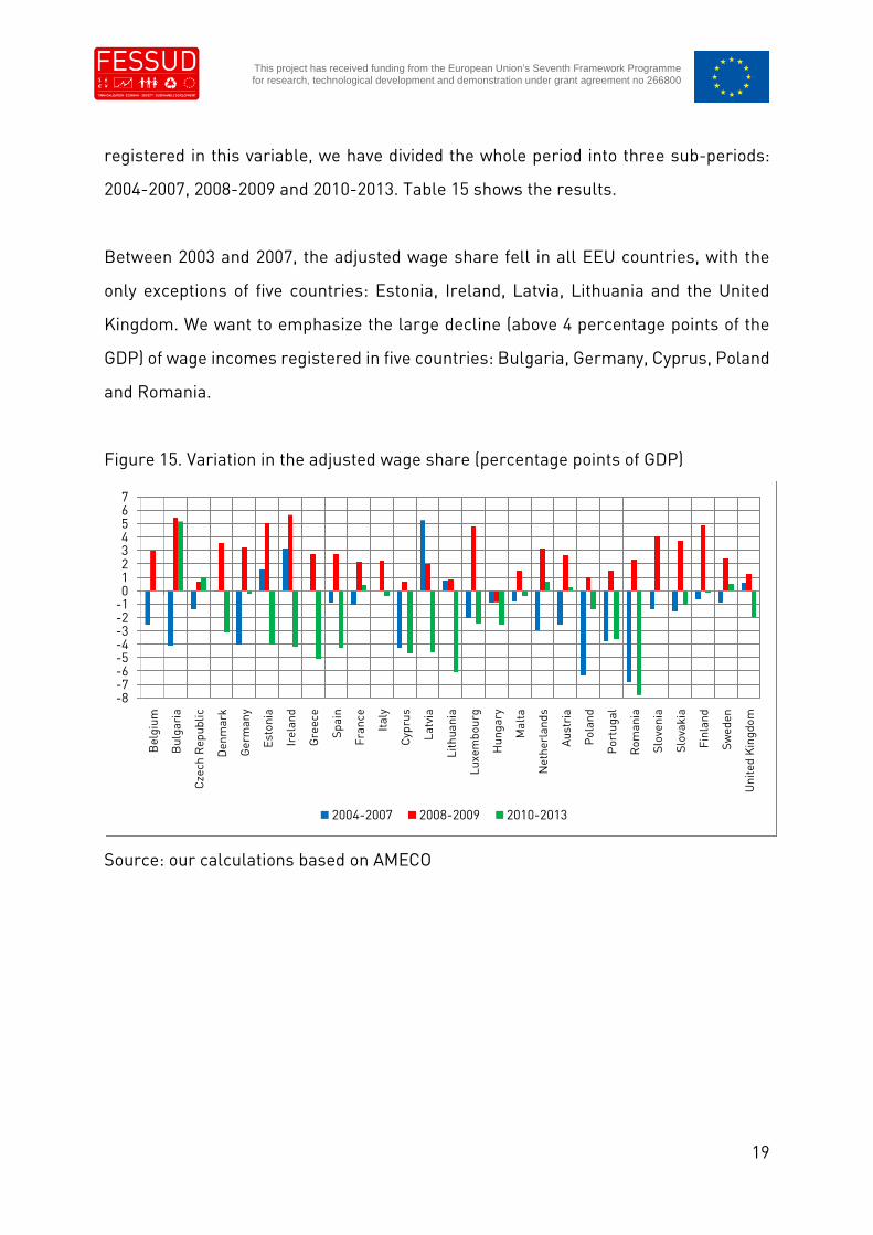
registered in this variable, we have divided the whole period into three sub-periods:

2004-2007, 2008-2009 and 2010-2013. Table 15 shows the results.

Between 2003 and 2007, the adjusted wage share fell in all EEU countries, with the

only exceptions of five countries: Estonia, Ireland, Latvia, Lithuania and the United

Kingdom. We want to emphasize the large decline (above 4 percentage points of the

GDP) of wage incomes registered in five countries: Bulgaria, Germany, Cyprus, Poland

and Romania.

Figure 15. Variation in the adjusted wage share (percentage points of GDP)


-8-7-6-5-4-3-2-101234567

Bel

gium

Bul

gari

a

Cze

chR

epub

lic

Den

mar

k

Ger

man

y

Esto

nia

Irel

and

Gre

ece

Spai

n

Fran

ce

Ital

y

Cyp

rus

Latv

ia

Lith

uani

a

Luxe

mbo

urg

Hun

gary

Mal

ta

Net

herl

ands

Aus

tria

Pol

and

Por

tuga

l

Rom

ania

Slov

enia

Slov

akia

Finl

and

Swed

en

Uni

ted

Kin

gdom

2004-2007 2008-2009 2010-2013

20


Figure 16. Variation of the adjusted wage share between 2007 and 2013 (% of GDP)


This pattern reversed at the beginning of the crisis. Thus, with the only exception of

Hungary, the adjusted wage share increased noticeably, a proof that, at a first stage,

(real) wages and employment were not seriously affected by the crisis. The scene is

dramatically different since 2010. Between 2010 and 2013, the adjusted wage share

has declined in nineteen countries, and in eight countries (Estonia, Ireland, Greece,

Spain, Cyprus, Latvia, Lithuania and Romania) the decline exceeds 4 per cent of the

GDP. As a result of this process, the adjusted wage share as declined since the year

2008 in ten countries (see figure 16).

The second analysis of income distribution is based on the Gini coefficient of

equivalised disposable income. Figure 17 shows the large differences existing in the

European Union related to the income distribution, both before and after the burst of

the financial crisis in 2008. Five countries registered a Gini coefficient below 26:

Slovenia (23.2), Sweden (23.5), Denmark (24.3), Czech Republic (25.5) and Finland

(25.9). It is easy to see that the Scandinavian countries enjoyed the most egalitarian

income distribution in the European Union. On the contrary, the least egalitarian

income distribution happened in Italy and Romania (32.6), United Kingdom (33.4),

-6-4-202468

1012

Bul

gari

a

Finl

and

Slov

enia

Net

herl

ands

Ger

man

y

Bel

gium

Aus

tria

Swed

en

Slov

akia

Fran

ce

Luxe

mbo

urg

Ital

y

Cze

chR

epub

lic

Irel

and

Mal

ta

Esto

nia

Den

mar

k

Pol

and

Uni

ted

Kin

gdom

Spai

n

Por

tuga

l

Gre

ece

Latv

ia

Hun

gary

Cyp

rus

Lith

uani

a

Rom

ania

21


Poland (33.7), Greece (33.9), Estonia (34.4), Lithuania (35), Latvia (36.8), Portugal (37.6).

With the exception of the UK, the least egalitarian countries are Mediterranean and

central and eastern Europe.

Figure 17. Gini coefficient

Source: Our calculations based on Eurostat

The crisis has led to an increase in the income inequalities in eleven countries,

standing out above all the cases, Bulgaria where its Gini coefficient has risen in 6.1

points. The figure 17 confirms that the most and the least egalitarian countries remain,

with minor changes, basically the same. However, if we want to know how much the

crisis has impacted on the personal income distribution in the EU, it is better to look

at figure 18, that shows the changes registered in the Gini coefficients between 2008

and 2013.

Figure 18. Change in the Gini coefficient between 2008 and 2013

20222426283032343638

Bel

gium

Bul

gari

a

Cze

chR

epub

lic

Den

mar

k

Ger

man

y

Esto

nia

Irel

and

Gre

ece

Spai

n

Fran

ce

Ital

y

Cyp

rus

Latv

ia

Lith

uani

a

Luxe

mbo

urg

Hun

gary

Mal

ta

Net

herl

ands

Aus

tria

Pol

and

Por

tuga

l

Rom

ania

Slov

enia

Slov

akia

Finl

and

Swed

en

Uni

ted

Kin

gdom

2003-2007 2008-2013

22



Since the onset of the financial crisis, the income distribution is more egalitarian in 13

countries. It is remarkable the fact that four of the five countries that has registered

the highest decline in the Gini coefficient were, precisely, the countries with the least

egalitarian income in the EU (Poland, Portugal, Romania and the United Kingdom). The

worst performance, on the contrary, is registered in France, Luxembourg, Cyprus,

Hungary and Denmark. With the exception of Denmark, these countries were not

among those with the more egalitarian income distribution. Therefore, we can state

that the crisis, in general has not had a significant negative impact on those countries

that before the crisis has a more egalitarian income distribution.

2.4 Inflation

Figure 19 shows the evolution of inflation rate, measured by the Consumer Price Index

(CPI) in the European Union. The most remarkable fact is that before the crisis, the

most inflationary economies were those that at that time were not member of the

Eurozone. It is surprising that the average annual inflation rate after 2008 has only

been lower than that registered in the period 2003-2007 in 11 countries. However, this

-4-3-2-101234

Fran

ce

Luxe

mbo

urg

Cyp

rus

Hun

gary

Den

mar

k

Spai

n

Mal

ta

Swed

en

Slov

enia

Lith

uani

a

Aus

tria

Ital

y

Bul

gari

a

Gre

ece

Latv

ia

Slov

akia

Bel

gium

Esto

nia

Cze

chR

epub

lic

Ger

man

y

Finl

and

Irel

and

Pol

and

Uni

ted

Kin

gdom

Net

herl

ands

Por

tuga

l

Rom

ania

23


result is explained by the hike registered in the inflation rate in the year 2008: in this

year the inflation rate accelerated in 25 EU countries.

Figure 19. Average annual inflation rate (%)

Source: Our calculations based on AMECO

Figure 20. Average annual inflation rate for the periods 2003-2007 and 2009-2013 (%)


0123456789

10

Bel

gium

Bul

gari

a

Cze

chR

epub

lic

Den

mar

k

Ger

man

y

Esto

nia

Irel

and

Gre

ece

Spai

n

Fran

ce

Ital

y

Cyp

rus

Latv

ia

Lith

uani

a

Luxe

mbo

urg

Hun

gary

Mal

ta

Net

herl

ands

Aus

tria

Pol

and

Por

tuga

l

Rom

ania

Slov

enia

Slov

akia

Finl

and

Swed

en

Uni

ted

Kin

gdom

2003-2007 2008-2013

-10123456789

10

Bel

gium

Bul

gari

a

Cze

chR

epub

lic

Den

mar

k

Ger

man

y

Esto

nia

Irel

and

Gre

ece

Spai

n

Fran

ce

Ital

y

Cyp

rus

Latv

ia

Lith

uani

a

Luxe

mbo

urg

Hun

gary

Mal

ta

Net

herl

ands

Aus

tria

Pol

and

Por

tuga

l

Rom

ania

Slov

enia

Slov

akia

Finl

and

Swed

en

Uni

ted

Kin

gdom

2003-2007 2009-2013

24


To avoid this problem, in figure 20 we show the average annual inflation rates for the

periods 2003-2007 and 2009-2013. Now it is more evident the disinflationary impact of

the Great Recession, mainly in the most inflationary countries before the crisis.

Figure 21. Variation of inflation rate between 2007 and 2013 (percentage points)


However, even with the removal of the year 2008, the inflation rates have been higher

since 2009 than before the crisis (Denmark, Lithuania, Netherlands, Austria, Poland,

Finland and the United Kingdom). This result is due to the fact that in most countries

the inflation rates were declining since 2009.

Thus, when we calculate the change in the inflation rates registered between 2007 and

2013, as we show in figure 21, we can better appreciate the disinflationary impact of

the financial crisis. Thus, in four countries the inflation rate in the year 2013 was higher

than in 2007. In the rest of EU countries the inflation rate was lower in 2013.

-11-10

-9-8-7-6-5-4-3-2-101

Net

herl

ands

Uni

ted

Kin

gdom

Mal

ta

Aus

tria

Luxe

mbo

urg

Fran

ce

Ital

y

Bel

gium

Ger

man

y

Rom

ania

Den

mar

k

Finl

and

Spai

n

Cze

chR

epub

lic

Slov

akia

Pol

and

Slov

enia

Por

tuga

l

Swed

en

Cyp

rus

Esto

nia

Gre

ece

Irel

and

Lith

uani

a

Hun

gary

Bul

gari

a

Latv

ia

25


2.5 Balance on current transactions

The situation of the balances on current transactions of EU countries was

characterized in the years before the crisis by a generalized negative balance. As figure

22 shows, in the years 2003-2007, only eight countries recorded a surplus in the

balance on current transactions: Belgium, Denmark, Germany, Luxembourg,

Netherland, Austria, Finland and Sweden. Out of these countries, in five countries the

surplus on current transactions exceeded 4 per cent of GDP: Finland, 4.3%), Germany

(4.7%), Netherlands (7%), Sweden (7.6%) and Luxembourg (10.6%). In the case of

deficit countries, 13 economies registered deficits above 4% of GDP, standing out the

cases of four countries, whose average annual deficits exceeded 10% of GDP: Greece

(11.7% of GDP), Bulgaria and Estonia (13% of GDP) and Latvia (-15.3 of GDP.

Figure 22. Average balance on current transactions (% of GDP)


The Great Recession, and the consequent decline in the economic activity and the

aggregate demand, has led to a substantial improvement in the balance on current

transactions. Although in the period 2008-2013, only nine countries register surpluses

-16-14-12-10

-8-6-4-202468

1012

Bel

gium

Bul

gari

a

Cze

chR

epub

lic

Den

mar

k

Ger

man

y

Esto

nia

Irel

and

Gre

ece

Spai

n

Fran

ce

Ital

y

Cyp

rus

Latv

ia

Lith

uani

a

Luxe

mbo

urg

Hun

gary

Mal

ta

Net

herl

ands

Aus

tria

Pol

and

Por

tuga

l

Rom

ania

Slov

enia

Slov

akia

Finl

and

Swed

en

Uni

ted

Kin

gdom

2003-2007 2008-2013

26


in the balance on current transactions, in 18 countries there is an improvement in the

balance on current transactions. Out of the other 9 countries, in four countries

(Belgium, Luxembourg, Finland and Sweden), the crisis has come with a decline in

their respective surpluses, in four countries there has been an increase of the balance

on current transactions (France, Italy, Cyprus, Poland and the United Kingdom).

Figure 23. Variation of the balance on current transactions between 2007 and 2013 (%of GDP)


It is important to emphasize that eight countries which, on average, have recorded a

deficit in the balance on current transactions over the years 2003 to 2013, in the year

2013 have registered a surplus in the balance on current transactions: Bulgaria,

Ireland, Spain, Italy, Lithuania, Hungary, Malta and Slovakia.

In this sense, the figure 23 allows a better understanding of the dimension of the

adjustment in the balance on current transactions that has happened during the Great

Recession. Only in eight countries, there has been a worsening in the balance on

current transactions, standing out the substantial worsening that has taken place in

Luxembourg, Belgium and Finland (above 5 per cent of the GDP). On the contrary, in

-10

-5

0

5

10

15

20

25

30

Bul

gari

a

Latv

ia

Lith

uani

a

Esto

nia

Gre

ece

Rom

ania

Hun

gary

Spai

n

Irel

and

Por

tuga

l

Cyp

rus

Slov

enia

Mal

ta

Slov

akia

Den

mar

k

Pol

and

Cze

chR

epub

lic

Ital

y

Net

herl

ands

Ger

man

y

Fran

ce

Aus

tria

Uni

ted

Kin

gdom

Swed

en

Luxe

mbo

urg

Bel

gium

Finl

and

27


twelve countries the improvement in the external balance exceeds 8 per cent of the

GDP.

2.6 Public finances

To analyze the impact of the crisis on the public finances of EU countries we will focus

on two variables related to the size of fiscal imbalances: the public budget balance and

the public debt, both variables being measured as percentages of the GDP.

Figure 24 shows the evolution of the public budget balances since 2003. During the

pre-crisis years, most EU countries registered deficits in their public finances. The

only exceptions were Bulgaria, Denmark, Estonia, Ireland, Spain, Luxembourg,

Finland and Sweden. Out of the 19 deficit countries, in nine countries the fiscal deficit

was above 3 per cent of the GDP (Czech Republic, Greece, France, Italy, Hungary,

Malta, Poland, Portugal and United Kingdom). It must be noticed that in 2007 there was

a generalized deterioration in the situation of public finances in the EU that affected to

24 countries, and thus only in three countries (Austria, Germany and Netherlands) the

public budget balance improved in 2007

Figure 24. Public budget balances (% of GDP)

28



The burst of the crisis led to a strong deterioration of public finances. Thus, in the years

2008 and 2009 only four countries (Denmark, Luxembourg, Finland and Sweden)

generated a fiscal surplus In 17 countries the fiscal deficits were exceeded the 3 per

cent of the GDP; standing out the cases of Ireland (10.6% of GDP) and Greece (12.8%).

Figure 25. Change in the public budget balance in 2008 and 2009 (% of GDP)


Figure 25 shows the accumulated impact of the crisis on the public budget balance

(PBB) in the years 2008 and 2009. We have calculated the difference between the PBB

-16-14-12-10

-8-6-4-2024

Bel

gium

Bul

gari

a

Cze

chR

epub

lic

Den

mar

k

Ger

man

y

Esto

nia

Irel

and

Gre

ece

Spai

n

Fran

ce

Ital

y

Cyp

rus

Latv

ia

Lith

uani

a

Luxe

mbo

urg

Hun

gary

Mal

ta

Net

herl

ands

Aus

tria

Pol

and

Por

tuga

l

Rom

ania

Slov

enia

Slov

akia

Finl

and

Swed

en

Uni

ted

Kin

gdom

2003-2007 2008-2009 2010-2013

-14

-12

-10

-8

-6

-4

-2

0

2

Hun

gary

Mal

ta

Aus

tria

Ger

man

y

Ital

y

Esto

nia

Luxe

mbo

urg

Swed

en

Fran

ce

Cze

chR

epub

lic

Bel

gium

Bul

gari

a

Pol

and

Net

herl

ands

Rom

ania

Slov

akia

Slov

enia

Por

tuga

l

Den

mar

k

Finl

and

Latv

ia

Lith

uani

a

Uni

ted

Kin

gdom

Gre

ece

Cyp

rus

Spai

n

Irel

and

29


registered in 2009 and that of the year 2007. With the exception of Hungary, whose

public finances registered and improvement, all the EU countries saw how their public

finances suffered a strong deterioration, standing out the cases of Greece, Cyprus,

Spain and Ireland.

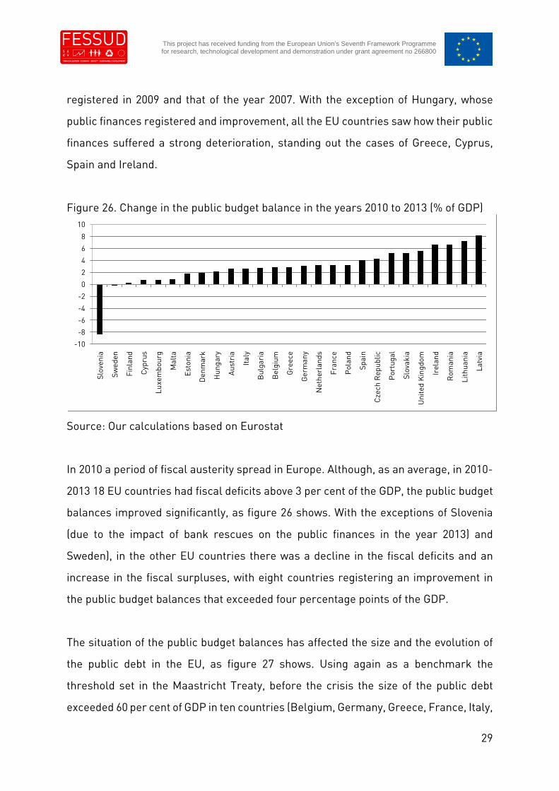
Figure 26. Change in the public budget balance in the years 2010 to 2013 (% of GDP)


In 2010 a period of fiscal austerity spread in Europe. Although, as an average, in 2010-

2013 18 EU countries had fiscal deficits above 3 per cent of the GDP, the public budget

balances improved significantly, as figure 26 shows. With the exceptions of Slovenia

(due to the impact of bank rescues on the public finances in the year 2013) and

Sweden), in the other EU countries there was a decline in the fiscal deficits and an

increase in the fiscal surpluses, with eight countries registering an improvement in

the public budget balances that exceeded four percentage points of the GDP.

The situation of the public budget balances has affected the size and the evolution of

the public debt in the EU, as figure 27 shows. Using again as a benchmark the

threshold set in the Maastricht Treaty, before the crisis the size of the public debt

exceeded 60 per cent of GDP in ten countries (Belgium, Germany, Greece, France, Italy,

-10

-8

-6

-4

-2

0

2

4

6

8

10

Slov

enia

Swed

en

Finl

and

Cyp

rus

Luxe

mbo

urg

Mal

ta

Esto

nia

Den

mar

k

Hun

gary

Aus

tria

Ital

y

Bul

gari

a

Bel

gium

Gre

ece

Ger

man

y

Net

herl

ands

Fran

ce

Pol

and

Spai

n

Cze

chR

epub

lic

Por

tuga

l

Slov

akia

Uni

ted

Kin

gdom

Irel

and

Rom

ania

Lith

uani

a

Latv

ia

30


Cyprus, Hungary, Malta, Austria and Poland). It is striking the fact, that with the

exception of Hungary, the highest indebted countries belonged to the Eurozone.

Figure 27. Public debt (% of GDP)


Figure 28. Accumulated increase in the size of public debt between 2007 and 2013 (%of GDP)


The deterioration in the public budget balances has implied that in the post-period

crisis the size of the public debt is larger than in the period 2003-2007 (with the only

020406080

100120

140160

Bel

gium

Bul

gari

a

Cze

chR

epub

lic

Den

mar

k

Ger

man

y

Esto

nia

Irel

and

Gre

ece

Spai

n

Fran

ce

Ital

y

Cyp

rus

Latv

ia

Lith

uani

a

Luxe

mbo

urg

Hun

gary

Mal

ta

Net

herl

ands

Aus

tria

Pol

and

Por

tuga

l

Rom

ania

Slov

enia

Slov

akia

Finl

and

Swed

en

Uni

ted

Kin

gdom

2003-2007 2008-2013

0102030405060708090

100

Irel

and

Gre

ece

Por

tuga

l

Spai

n

Cyp

rus

Slov

enia

Uni

ted

Kin

gdom

Latv

ia

Ital

y

Fran

ce

Net

herl

ands

Rom

ania

Slov

akia

Lith

uani

a

Finl

and

Cze

chR

epub

lic

Den

mar

k

Bel

gium

Aus

tria

Luxe

mbo

urg

Ger

man

y

Pol

and

Hun

gary

Mal

ta

Esto

nia

Bul

gari

a

Swed

en

31


exception of Bulgaria). However, the figure 27 does not give a correct picture of the

huge increase registered in the public debt in most countries, because, as mentioned,

it shows the average of the two sub-periods, thus hiding the rising trend registered in

most countries

To avoid this problem in the figure 28 we show the change registered in the size of

public debt between the years 2008 and 2013. In seven countries, the increase in the

stock of public debt is below 15 per cent of the GDP (Germany, Poland, Hungary, Malta,

Estonia, Poland and Sweden). On the contrary, the increase in the stock of public debt

is above 40 per cent of the GDP in seven countries (Ireland, Greece, Portugal, Spain,

Cyprus, Slovenia and United Kingdom), with six of these countries belonging to the

euro.

2.7 Financial balance sheets

This sub-section will analyze the impact of the crisis on the size of the financial assets,

financial liabilities and net financial liabilities of the total economy, that is, we will not

make a disaggregated analysis by sectors. Like in the precious section, the source of

the data is Eurostat. The data analyzed refer to the period 2003-2012, because at the

time of elaborating this deliverable data about all EU countries were not available. The

analysis does not include Luxembourg due both to the lack of available data before the

year 2007 and to the huge size in this country of the financial assets and liabilities (6

times larger than the second country in terms of the size of the financial assets and

liabilities measured as a percentage of the GDP).

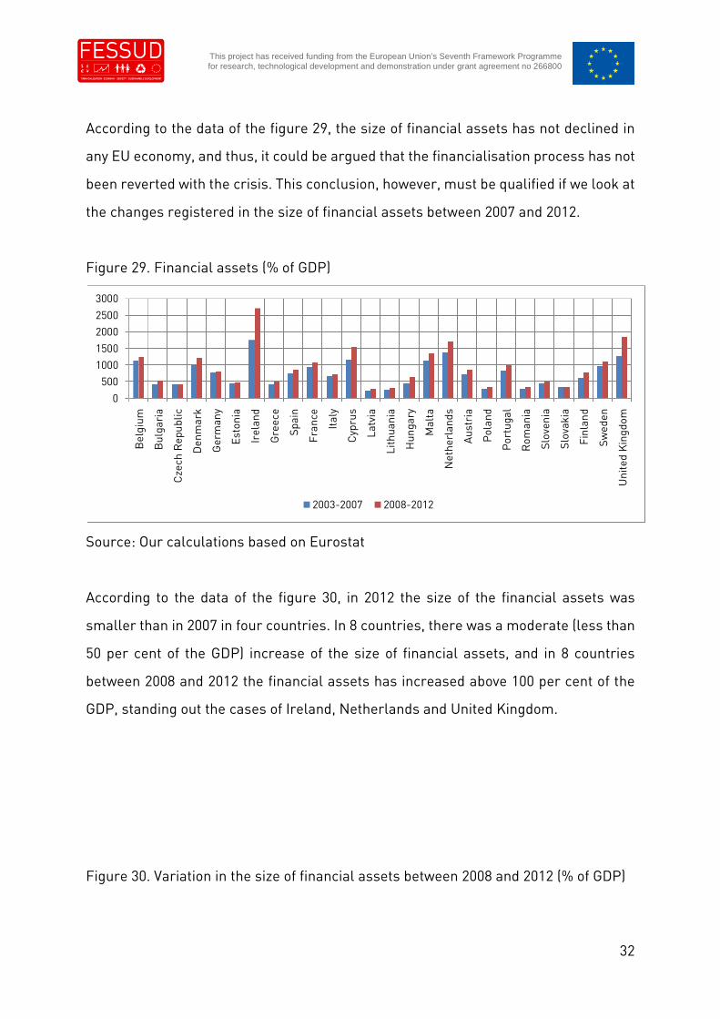
Figure 29 shows the size of the financial assets in the total economy of the EU-27

countries. The figure shows the remarkable differences in the size of financial assets

both before and during the financial and economic crisis, where the smallest size of

the financial assets is registered in the central and eastern European countries.

32


According to the data of the figure 29, the size of financial assets has not declined in

any EU economy, and thus, it could be argued that the financialisation process has not

been reverted with the crisis. This conclusion, however, must be qualified if we look at

the changes registered in the size of financial assets between 2007 and 2012.

Figure 29. Financial assets (% of GDP)


According to the data of the figure 30, in 2012 the size of the financial assets was

smaller than in 2007 in four countries. In 8 countries, there was a moderate (less than

50 per cent of the GDP) increase of the size of financial assets, and in 8 countries

between 2008 and 2012 the financial assets has increased above 100 per cent of the

GDP, standing out the cases of Ireland, Netherlands and United Kingdom.

Figure 30. Variation in the size of financial assets between 2008 and 2012 (% of GDP)

0

50010001500

20002500

3000

Bel

gium

Bul

gari

a

Cze

chR

epub

lic

Den

mar

k

Ger

man

y

Esto

nia

Irel

and

Gre

ece

Spai

n

Fran

ce

Ital

y

Cyp

rus

Latv

ia

Lith

uani

a

Hun

gary

Mal

ta

Net

herl

ands

Aus

tria

Pol

and

Por

tuga

l

Rom

ania

Slov

enia

Slov

akia

Finl

and

Swed

en

Uni

ted

Kin

gdom

2003-2007 2008-2012

33



Similar conclusions are obtained when we analyze the evolution of the financial

liabilities of the total economy (see figures 31 and 32).

Figure 31. Financial liabilities (% of GDP)


Figure 32. Variation in the size of financial liabilities between 2008 and 2012 (% of GDP)

-1000

100200300400500600700800

Irel

and

Net

herl

ands

Uni

ted

Kin

gdom

Finl

and

Mal

ta

Por

tuga

l

Cyp

rus

Den

mar

k

Hun

gary

Gre

ece

Swed

en

Spai

n

Ital

y

Cze

chR

epub

lic

Fran

ce

Pol

and

Slov

akia

Ger

man

y

Aus

tria

Lith

uani

a

Latv

ia

Slov

enia

Bel

gium

Bul

gari

a

Rom

ania

Esto

nia

0

500

1000

1500

2000

2500

3000

Bel

gium

Bul

gari

a

Cze

chR

epub

lic

Den

mar

k

Ger

man

y

Esto

nia

Irel

and

Gre

ece

Spai

n

Fran

ce

Ital

y

Cyp

rus

Latv

ia

Lith

uani

a

Hun

gary

Mal

ta

Net

herl

ands

Aus

tria

Pol

and

Por

tuga

l

Rom

ania

Slov

enia

Slov

akia

Finl

and

Swed

en

Uni

ted

Kin

gdom

2003-2007 2008-2012

34



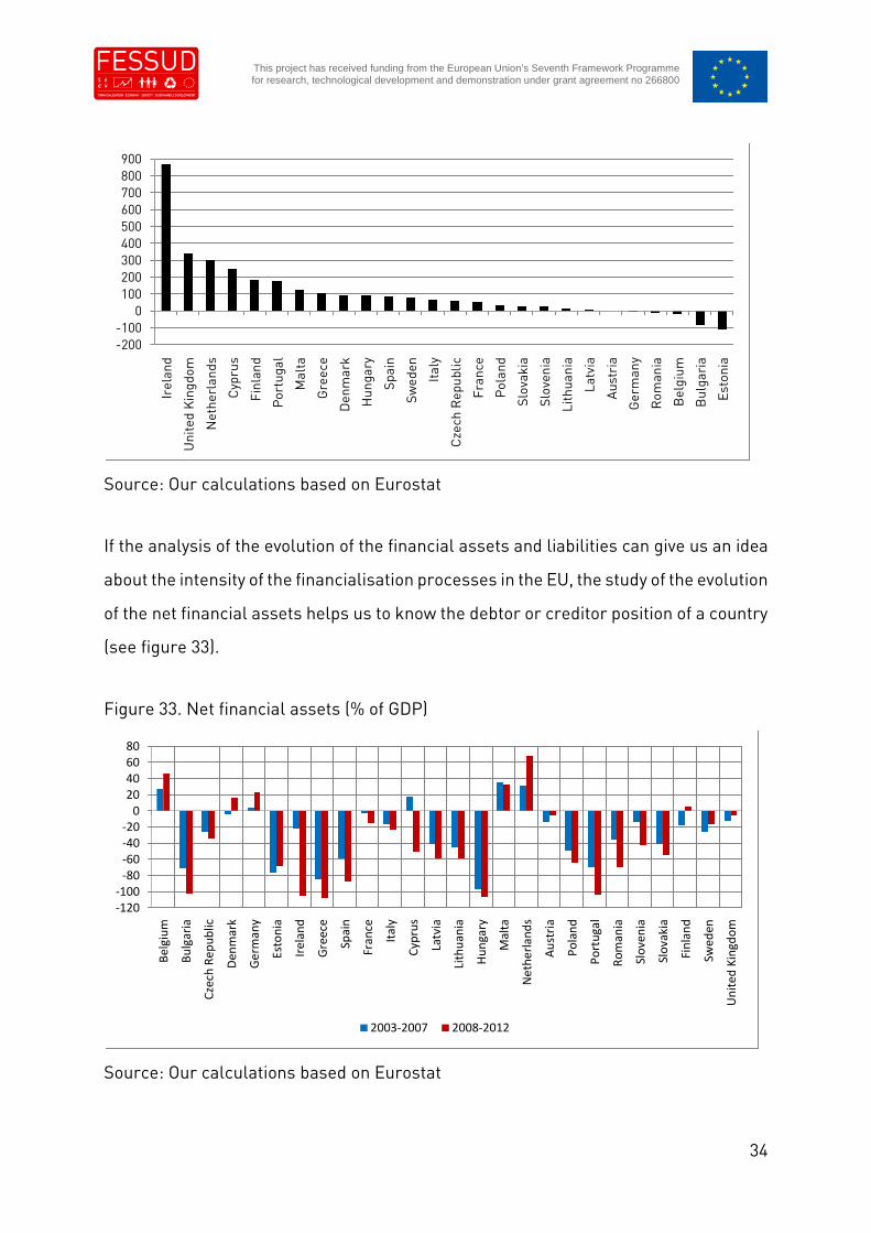
If the analysis of the evolution of the financial assets and liabilities can give us an idea

about the intensity of the financialisation processes in the EU, the study of the evolution

of the net financial assets helps us to know the debtor or creditor position of a country

(see figure 33).

Figure 33. Net financial assets (% of GDP)


-200-100

0100200300400500600700800900

Irel

and

Uni

ted

Kin

gdom

Net

herl

ands

Cyp

rus

Finl

and

Por

tuga

l

Mal

ta

Gre

ece

Den

mar

k

Hun

gary

Spai

n

Swed

en

Ital

y

Cze

chR

epub

lic

Fran

ce

Pol

and

Slov

akia

Slov

enia

Lith

uani

a

Latv

ia

Aus

tria

Ger

man

y

Rom

ania

Bel

gium

Bul

gari

a

Esto

nia

-120-100

-80-60-40-20

020406080

Bel

giu

m

Bu

lgar

ia

Cze

chR

epu

blic

Den

mar

k

Ge

rman

y

Esto

nia

Irel

and

Gre

ece

Spai

n

Fran

ce

Ital

y

Cyp

rus

Latv

ia

Lith

uan

ia

Hu

nga

ry

Mal

ta

Ne

the

rlan

ds

Au

stri

a

Po

lan

d

Po

rtu

gal

Ro

man

ia

Slo

ven

ia

Slo

vaki

a

Fin

lan

d

Swed

en

Un

ited

Kin

gdo

m

2003-2007 2008-2012

35


Before the crisis, only five countries had a creditor financial position: Belgium,

Germany, Cyprus, Malta and Netherlands. The other 21 countries had a debtor

position, standing out the cases of Bulgaria, Estonia, Greece, Spain, Hungary and

Portugal. In the crisis period, only 6 countries registered a creditor financial position:

Belgium, Denmark, Germany, Malta, Netherlands and Finland. But, and being more

important, only five countries registered during the crisis an improvement (small

debtor position or larger creditor position) in their financial position: Netherlands,

Austria, Finland, Sweden and the United Kingdom.

Figure 34. Variation in the size of net financial assets between 2008 and 2012 (% ofGDP)


To avoid the problem generated by working with averages, in the figure 34 we show

the variation in the financial position between 2008 and 2012. A positive value implies

an improvement in the financial position, and vice versa. In twelve out of the 26

countries there is a strong deterioration of the financial position, mainly in the cases

of Ireland and Cyprus. On the contrary, there is a significant improvement (more than

20 per cent of the GDP) in the financial position of Bulgaria, Denmark. Netherlands,

Finland, Malta and Germany.

-120-100

-80-60-40-20

0204060

Bul

gari

a

Den

mar

k

Net

herl

ands

Finl

and

Mal

ta

Ger

man

y

Esto

nia

Bel

gium

Aus

tria

Latv

ia

Hun

gary

Ital

y

Lith

uani

a

Uni

ted

Kin

gdom

Swed

en

Cze

chR

epub

lic

Pol

and

Slov

akia

Spai

n

Fran

ce

Gre

ece

Slov

enia

Por

tuga

l

Rom

ania

Irel

and

Cyp

rus

36


2.8 Conclusions

The analysis of the selected economic (real and financial variables) shows that, in

general, the countries that have had a worst performance during the Great Recession

have been the new member states of the Eurozone, that is those that join the euro after

its creation in 1999. Out of those countries that joined the European Monetary Union in

the year 1999, it is Spain the country that registers the deepest impact of the crisis.

Regarding those countries that are not part of the Eurozone (EU-10), it must be

emphasized that the larger impact of the crisis is registered in two countries, Latvia

and Lithuania, which are nowadays part of the Eurozone.

These results show that the crisis in the European Union is basically a crisis of the

Eurozone, but that even in this area there are different effects, with the new member

states and the peripheral countries, mainly Spain, being the most affected countries.

This allows to concluding that, although the origin of the crisis is the same for the

whole EU, there some circumstances in certain economies that make that the impact

of this common shock has been more severe in these economies.

3. The impact of the crisis on the coherence of the Eurozone

Even before the creation of the European Monetary Union, it was commonly argued

that member states did not form an optimum currency area. By focusing the

convergence requirements into variables of nominal nature, there was no guarantee

that the members that joined, at a first stage or later, the Eurozone achieved a

sufficient real convergence that gave rise to a high synchronization of the national

business cycles, thus avoiding the problems due to the problem of the loss of

autonomy in key areas of the macroeconomic policy, namely the monetary policy and

the loss of the tool of the exchange rate. However, defenders of the process of

37


monetary integration argued that real convergence would be a (medium or long-term)

consequence of the monetary unification (Mongelli, 2013; Gibson, Palivos and Tavlos,

2014).

Therefore, this strategy of creation and subsequent enlargement of the European

Monetary Union implied that the Eurozone was, in an (highly) optimistic view, at least

in the first years of its creation, more prone to suffer asymmetric shocks: that is,

countries could be at different phases of the business cycle (mainly explained by the

existence of domestic shocks), or the intensity (duration) of the booms-busts could be

significantly different (due to the very domestic shocks or because common shocks

could have different impact on the member states).

This problem is more serious if the heterogeneity is not corrected with the time, that

is, if the asymmetric shocks are not temporary but permanent. In other words, if the

desired process of real convergence among the monetary union member states does

not take place or takes longer time than expected1.

This is an even greater problem if the monetary union (or the individual member

states) does not have tools to correct or absorb these shocks, regardless whether it

means that common economic policies are not able to absorb the domestic shocks or

that national economic policies lacks of the required flexibility to correct the deviations

of the domestic business cycle.

Recent literature offers mixed conclusions about the evolution of the heterogeneity of

the Eurozone and the synchronization of the national business cycles. Cavallo and

Ribba (2015), conclude, analyzing eight euro countries, that there exists a significant

macroeconomic heterogeneity in the euro area, where the business cycles of some

1 Obviously this problem increases if there is an enlargement process in monetary union, inwhich the new member states differ significantly of the incumbent ones.

38


countries like Greece, Ireland or Portugal are mainly dominated by local shocks.

Ferroni and Klaus (2015) show a decoupling of Spain of Germany and France. Benzces

and Szent-Ivanyi (2015) argue that there was a convergence process in the European

economies that, however, was reversed after the onset of the economic and financial

crisis. Finally, contrary to these views, Gächter and Riedl (2014) argue that the

introduction of the euro has led to a higher correlation of the business cycles of the

member states, increasing the symmetry of national business cycles.

The analysis of the previous section has clearly shown that the economic and financial

crisis, a shock that can be defined as a common shock for the EU, in general, and the

Eurozone, in particular, has had a different impact in the Member states of both areas.

Regarding the European Monetary Union, the doubt would be whether this differential

effect is purely accidental or, on the contrary, it is the result of a structural behavior

of the Eurozone that proves the existence and the importance of the asymmetric

shocks in the Euro area.

As Carrasco et al. (2016) shows, the different impacts of the Great Recession on the

“old” and “new” euro economies emphasizes the problems of consistency in the

enlargement process of the European Monetary Union, as far as this enlargement

implies greater (macro)economic heterogeneity and increased coordination problems

with (possibly) more frequent asymmetric shocks.

The objective of this section is to analyse the coherence of the Eurozone, understood

as the macroeconomic performance heterogeneity of the euro member states. To be

more precise, our analysis has a dynamic nature. We will analyse whether since the

creation of the European Monetary Union the differences in the macroeconomic

performance of the members states have diminished, maintained, or, on the contrary,

it has increased.

39


3.1. Data and methodology

As mentioned in the previous section, in the section we have analysed the differences

in the economic performance of the Euro area member states. Namely, we have

focused our attention on the evolution of fourteen variables, related to six categories

of real (non-financial) variables:

1. Economic activity: real GDP per capita, real GDP growth rate, GDP per capita growth

rate, potential GDP growth rate, output gap

2. Labour market: employment growth rate, unemployment rate, real wages growth

rate, real unit labor costs growth rate

3. Income distribution: adjusted wage share (% of GDP), GINI coefficient

4. Inflation: inflation rate (CPI)

5. Balance of payments: balance on current account (% of GDP)

6. Public finances: public budget balance (% of GDP), public debt (% of GDP)

The data of these variables have been obtained in Eurostat and the AMECO database.

The period that we have analysed corresponds to the years 1995 to 2013, both included.

Since the last year analysed is 2013, we only analyse seventeen countries, excluding

Latvia and Lithuania, because these two countries joined the euro after this year.

Given that our interest is focused on the national differences existing in the values

registered in the fourteen countries, we have calculated, for the data available for each

year, the standard deviation of each macroeconomic variable. Once that for each

variable we have calculated the evolution of the standard deviation, our objective is to

detect the possible existence of a trend in the evolution of the standard deviation. Thus,

if we are able to detect a trend for this standard deviation to fall over the years, we will

be able to talk of the existence of a convergence process in this variable, but if we

40


detect a trend for this standard deviation to rise throughout the years, we will be able

to talk of the existence of a divergence process in this variable.

In sum, we are developing an analysis of sigma-convergence, where the objective is to

detect the existence of a trend in the evolution over the years of the standard deviation

of the values recorded of a variable in a group of individuals, in this case, countries.

Thus, we are making a regression of the standard deviation of a certain variable, where

the independent variable is a time trend:

StdDevt 0 1trend + ut (Equation 1)

1 is negative, therefore we can talk of the existence of

1 is positive, therefore we can talk

of the existence of a divergence process.

As far as the only independent variable, (besides the constant term) is the time trend,

equation 1 implies the analysis of a process of unconditional convergence, where time

is the only variable that explains the changes in the dependent variable. To detect other

potential determinants of the changes in the differences among individuals of the value

StdDevt 0 1trend + Xt + ut (Equation 2)

In equation 2, Xt is a vector of variables that can influence the change in the standard

variation of the variable in question. In our analysis we have included two different

variables that can constitute a proxy of the economic situation of the countries. The

first variable is called “recession”, and it is a dummy that tries to show the situation of

the Eurozone in the business cycle. Namely, the dummy recession takes the value 0 in

the boom phase of the business cycle, and 1 during the recession phase. The existence

41


of a recession (boom) has been determined by the value of the output gap of each

country in all the years analysed, where a negative output gap is identifies as a

recession and a positive output gap as an expansion. The value and the sign of the

output gap of the Eurozone for each country-year has been obtained as the unweighted

average of the national output gaps. The national output gaps have been obtained at

the AMECO database. Thus, the dummy recession take the value 1 in 9 years: 1995,

1996, 1997, 2003, 2009, 2010, 2011, 2012 and 2013.

The second variable tries to collect the impact of the Great Recession on the

convergence-divergence process of the macroeconomic performance in the Eurozone.

This variable is represented by a dummy called “recession” that takes the value 1

during the years 2009 to 2013 (and 0 between 1995 and 2008).

Therefore, our analysis tries to know whether the process or convergence (divergence)

in the macroeconomic performance in the euro area is influenced by the business

cycle of the Eurozone and whether the extraordinary nature, depth and length of the

current economic and financial crisis is generating an additional impact on the

macroeconomic performance of the euro member states, and, consequently on the

coherence of the Eurozone.

The differences in the national performance in the analysed variables, and, therefore,

in the convergence-divergence process of the Eurozone, however, can be affected by

the existence of extreme cases. This implies that the value of a variable recorded in

one country (or several countries) in a specific year can be significantly higher or lower

than that recorded in the rest of countries, and, consequently, generating a bias that

can influence the result of the analysis.

To avoid the bias generated by these extreme values, we have made two different

42


analysis we have included all the available data. In the second analysis we have

excluded those values (country-year) that can be considered as extreme values. To

define a value as an extreme value, we have made a box-plot analysis, and here for

each year the data considered as a far or close outlier will be defined as an extreme

value, and, therefore, excluded from the analysis.

2.2. Results

As mentioned in previous section, we have estimated by OLS the existence of a process

the macroeconomic performance of the 17 euro economies during the years 1995 to

2013. In this section, we will present and analyze the results of this analysis.

Figure 35 shows the evolution of the standard deviation of the rate of growth of real

GDP with and without outliers. The box plot analysis detected the existence of one

outlier or extreme value: Luxembourg, for the whole period 1995-2013. As expected,

as will happen in all variables), the exclusion of the extreme values makes that the

standard deviation of the economic growth in the Eurozone be less pronounced. Both

with and without Luxembourg, figure 35 shows a rising divergence in the real GDP per

capita within the Eurozone.

Figure 35. Standard deviation of real GDP per capita

43


7,000

8,000

9,000

10,000

11,000

12,000

13,000

14,000

15,000

1996 1998 2000 2002 2004 2006 2008 2010 2012

with outliers without outliers


The regression analysis has detected the existence of a process of conditional

divergence (see table 1). This divergence process is independent on the exclusion or

inclusion in the analysis of Luxembourg conditional to crisis and recessions. The

analysis shows that the diverging process is halted during recessions. Moreover, the

Great Recession has also led to a convergence in the real GDP per capita in the

Eurozone

44


Table 1. OLS regression of the standard deviation of real GDP per capitaModel 1

WithOutliers

Model 2WithoutOutliers

Model 3With

Outliers


Model 5With

Outliers


Model 7Model With

Outliers


C 20749(0.409)

8792(0.000)

10250(0.000)

9383(0.000)

11391(0.000)

8147(0.000)

10643(0.000)

7834(0.000)

Trend -283.2(0.719)

19.1720.729

342.98(0.000)

21.350(0.841)

213.86(0.000)

99.373(0.000)

307.28(0.000)

138.56(0.000)

Dcrisis -2484(0.000)

-567.159(0.002)

-1741.58(0.002)

-730.59(0.008)

Drecession -1335(0.000)

-686(0.000)

-565.19(0.034)

-363.19(0.020)

AR(1) 0.919(0.000)

1.152(0.000)

0.855(0.000)

AR(2) -0.384(0.117)

Mean dependent variable 12828 8873 12683 8794 12683 8717 12683 8717R2 0.910 0.896 0.917 0.954 0.876 0.877 0.935 0.923F-statistic 76.325

(0.000)37.375(0.000)

88.665(0.000)

97.071(0.000)

56.770(0.000)

57.160(0.000)

72.885(0.000)

60.043(0.000)

D-W 1.498 1.806 1.148 1.517 1.314 1.493 1.451 1.359Jarque-Bera 3.002

0.2221.875

(0.395)0.952

(0.621)0.061

(0.969)1.332

(0.513)8.661

(0.013)0.930

(0.627)0.049

(0.975)Breusch-Pagan-Godfrey 0.206

0.6550.990

(0.335)2.545

(0.109)0.734

(0.496)0.071

(0.931)0.348

(0.710)1.846

(0.178)0.721

(0.504)Breusch-Godfrey LM 1.099

(0.362)2.827

(0.102)1.356

(0.289)1.011

(0.392)0.876

(0.438)0.524

(0.602)0.349

(0.711)0.074

(0.526)p-values in parenthesis

45

This project has received funding from the Europeanfor research, technological development and

Figure 36 shows the evolution of the standard deviation of the real GDP growth

rates with and without outliers. The box plot analysis detected the existence of

the following outliers or extreme values: Ireland (1996, 1998, 1999 and 2000),

Estonia (1997, 2000, 2003, 2005, 2006, 2009 and 2011), Luxembourg (1999 and

2000), Slovakia (2000 and 2007), Greece (2010 and 2011) and Cyprus (2013).

Figure 36. Standard deviation of real GDP growth rates

0.5

1.0

1.5

2.0

2.5

3.0

3.5

95 96 97 98 99 00 01 02 03 04 05 06 07 08 09 10 11 12 13



Table 2 shows the regressions made in the eight models analysed (the same for

the fourteen variables): unconditional sigma-convergence with and without

outliers, and conditional sigma-convergence with and without outliers.

46


Table 2. OLS regression of the standard deviation of real GDP growth rateModel 1

With OutliersModel 2WithoutOutliers

Model 3With Outliers




Model 7Model With

Outliers

Model 8Without

Outliers #C 2.262

(0.000)1.619

(0.000)2.432

(0.000)1.580

(0.000)2.137

(0.000)1.583

(0.000)2.212

(0.000)1.026

(0.000)Trend 0.008

(0.650)0.013

(0.447)-0.027(0.297)

0.021(0.437)

0.001(0.935)

0.001(0.534)

-0.007(0.803)

0.072(0.000)

Dcrisis 0.589(0.086)

-0.134(0.692)

0.174(0.730)

-1.069(0.000)

Drecession 0.393(0.045)

0.111(0.568)

0.316(0.289)

0.689(0.000)

AR(1) -0.613(0.005)

AR(2) -0.786(0.003)

Mean dependent variable 2.336 1.737 2.336 1.737 2.336 1.737 2.336 1.706R2 0.012 0.034 0.182 0.044 0.237 0.054 0.243 0.678F-statistic 0.212

(0.650)0.064

(0.447)1.787

(0.199)0.368

(0.697)2.489

(0.114)0.460

(0.639)1.609

(0.229)4.633

(0.016)Wald-F statistic 20.910

(0.000)D-W 2.052 2.043 2.343 2.024 1.959 2.130 2.046 2.138Jarque-Bera 0.352

(0.838)1.581

(0.453)1.075

(0.584)1.611

(0.446)1.069

(0.585)1.196

(0.549)1.150

(0.562)0.891


(0.695)0.002

(0.963)0.311

(0.736)0.119

(0.887)0.075

(0.927)0.030

(0.969)1.184

(0.349)3.917


(0.946)0.571

(0.576)0.792

(0.471)0.609

(0.557)0.067

(0.934)0.840

(0.452)0.310

(0.738)0.187

(0.832)p-values in parenthesis# White Heteroskedasticity-consistent standard errors and covariance

47


Model 8 shows the existence of a significant conditional divergence process. This

divergence process takes place when extreme values are excluded of the

analysis and when the dummy variables related to the existence of a recession

and to the Great Recession are included in the equation. The model allows to

concluding that there is a divergence process when outliers are excluded and

that this divergence process accelerates when the Eurozone is in a recession.

However, the Great Recession has contributed to a strong decline of the

differences in the economic growth of euro countries.

The third variable related to the evolution of the GDP is the potential GDP growth

rate. In this case the box-plot analysis has detected the existence of the following

outliers: Ireland (in the years 1995 to 2001), Slovakia (2010 and 2011) and Greece

(2010 and 2011). A simple look to the figure 37 does not help to reach any

conclusion about the existence of a convergence or divergence process regarding

this variable.

Figure 37. Standard deviation of potential GDP growth rate

0.6

0.8

1.0

1.2

1.4

1.6

1.8

2.0

1996 1998 2000 2002 2004 2006 2008 2010 2012



48


49


Table 3. OLS regression of the standard deviation of potential GDP growth rateModel 1

With OutliersModel 2WithoutOutliers


#

Model 4Without

Outliers #


#

Model 6Without

Outliers #

Model 7Model WithOutliers #

Model 8Without

Outliers #C 1.697

(0.000)1.158

(0.002)1.700

(0.000)0.797

(0.000)1.697

(0.000)1.059

(0.000)1.675

(0.000)0.804

(0.000)Trend -0.025

(0.000)0.008

(0.758)-0.025(0.006)

0.058(0.000)

-0.027(0.000)

0.255(0.018)

-0.024(0.006)

0.057(0.002)

Dcrisis 0.005(0.942)

-0.605(0.006)

-0.050(0.570)

-0.593(0.045)


-0.272(0.021)

0.052(0.178)

-0.009(0.9371)

AR(1) 1.148(0.000)

0.547(0.084)

1.141(0.000)

1.107(0.000)

1.160(0.000)

AR(2) -0.793(0.001)

-0.793(0.002)

-0.813(0.000)

-0.821(0.001)


(0.000)4.726

(0.025)21.131(0.000)

9.050(0.002)

24.520(0.000)

4.962(0.021)

18.588(0.000)

5.659(0.008)

Wald F-statistics 0.074(0.788)

11.317(0.001)

5.540(0.014)

D-W 2.205 1.693 2.223 1.686 2.366 1.269 2.199 1.680Jarque-Bera 1.392

(0.498)0.513

(0.773)1.373

(0.503)1.032

(0.596)0.716

(0.698)0.324

(0.850)0.543

(0.761)1.015


(0.797)0.752

(0.398)0.057

(0.944)5.867

(0.012)3.357

(0.060)3.357

(0.060)5.325

(0.013)3.871


(0.537)1.561

(0.246)0.6670.534

2.116(0.157)

2.045(0.166)

2.045(0.166)

0.331(0.726)

2.301(0.139)

p-values in parenthesis

# White Heteroskedasticity-consistent standard errors and covariance

50


Table 3 shows the results of the different OLS regressions carried out. It must be

emphasized that the results are different depending on the inclusion or exclusion

of the extreme values. When all data are included in the analysis, we detect a

process of unconditional convergence. In this case, neither the existence of a

recession in the Eurozone or the Great Recession exert a significant impact on

this trend. However, the results are different when we exclude the outliers. Now,

we have detected a process of conditional divergence, with the existence of

recessions and the Great Recession leading to a convergence process. It is

important to mention that although by separate both dummies are significant,

when we include the two of them in the regression (model 8), only the dummy

related to the Great Recession remains significant, and its coefficient reaches a

high (negative) value, showing the deep and generalized impact of the crisis,

mainly in the countries with previous high GDP growth rates.

The final variable analyzed related to the evolution of the GDP is the output gap,

a variable that can be used as a proxy of the phase of the business cycle in each

euro country and, also, as a proxy of the depth of the business cycle.

In the case of the output gap, the box-plots have detected a high number of

extreme values or outliers: Estonia (1995, 1996, 1999, 2006, 2007, 2009 and 2010),

Slovakia (1997, 2000 to 2003, and 2007), Portugal (1999), Luxembourg (2000),

Spain (2011) and Greece (2011 to 2013).

In this case, it is a easy to detect in the figure 38 an increase over the years of the

standard deviation of the output gaps in the Eurozone, regardless we are included

or not the extreme values.

Figure 38. Standard deviation of output gap

51


1.0

1.5

2.0

2.5

3.0

3.5

4.0

1996 1998 2000 2002 2004 2006 2008 2010 2012



The regressions (table 4) show a significant process of unconditional divergence,

that takes place with and without outliers. Here, neither the existence of a

recession or the Great Recession exert a significant influence on this trend.

The next four variables are related to the performance of the labour markets in

the Eurozone. The first variable is the annual rate of growth of total employment.

The box-plot analysis has detected the existence of extreme values in seven

countries: Ireland (1998, 1999 and 2009, Estonia (1999 and 2011), Spain (2000,

2002 and 2005), Slovakia (2000 and 2009), Cyprus (2001 and 2007), Greece (2011

and 2012) and Luxembourg (2012).

52


Table 4. OLS regression of the standard deviation of output GDPModel 1

WithOutliers

Model 2Without

Outliers #

Model 3With

Outliers

Model 4Without

Outliers #

Model 5With

Outliers #

Model 6Without

Outliers #

Model 7Model With

Outliers

Model 8Without

Outliers #C 0.832

(0.243)1.083

(0.000)0.795

(0.323)1.043

(0.000)0.838

(0.260)1.077

(0.000)0.783

(0.344)0.912

(0.000)Trend 0.131

(0.032)0.048

(0.005)0.136

(0.081)0.056

(0.000)0.130

(0.051)0.048

(0.003)0.137

(0.090)0.068

(0.000)Dcrisis -0.058

(0.914)-0.136(0.575)

-0.108(0.873)

-0.383(0.232)


0.018(0.836)

0.047(0.895)

0.158(0.217)

AR(1) 0.018(0.016)

0.542(0.019)


(0.000)14.964(0.000)

8.292(0.002)

7.331(0.005)

8.284(0.002)

7.057(0.006)

5.787(0.006)

5.037(0.013)


11.987(0.000)

8.771(0.002)

9.267(0.001)

D-W 1.793 1.716 1.836 1.776 1.774 1.741 1.816 1.806Jarque-Bera 0.746

(0.688)2.229

(0.327)0.736

(0.691)1.044

(0.593)0.747

(0.688)2.570

(0.276)0.733

(0.692)1.547


0.1667.338

(0.014)1.175

(0.305)5.795

(0.012)1.126

(0.350)4.382

(0.030)0.761

(0.534)3.574


(0.576)1.363

(0.285)0.504

(0.616)1.414

(0.275)0.568

(0.580)1.316

(0.299)0.476

(0.630)2.261


53


A look to figure 39 could lead to the conclusion that there has been a divergence

process regarding the evolution of total employment in the euro economies.

However, this conclusion is far from being so evident.

Figure 39. Standard deviation of the annual total employment growth rates

0.5

1.0

1.5

2.0

2.5

3.0

3.5

4.0

1996 1998 2000 2002 2004 2006 2008 2010 2012



Thus, the data of table 5 show that we could talk of a divergence process when

all the data are included. However, if we exclude the outliers of the analysis, we

cannot find any significant trend.

The results change dramatically when we make the analysis of conditional

sigma-convergence including separately in the regressions the dummy variables

recessions and the Great Recession (models 3 to 6). Here, there is no significant

trend in the evolution of the standard deviation of the rate of growth of total

employment, but both dummies are significant (with and without outliers). Thus,

both recessions and the Great Recession are leading to a higher divergence in

the evolution of total employment, being higher the impact of the Great

Recession.

54


Table 5. OLS regression of the standard deviation of total employment growth rateModel 1

WithOutliers


Model 3With

Outliers


Model 5With

Outliers


Model 7Model With

Outliers


C 1.506(0.000)

1.350(0.001)

1.993(0.000)

1.752(0.000)

1.324(0.000)

1.146(0.000)

2.272(0.000)

1.697(0.000)

Trend 0.051(0.083)

0.038(0.1653)

-0.051(0.102)

-0.046(0.156)

0.041(0.136)

0.026(0.268)

-0.076(0.048)

-0.042(0.3081)

Dcrisis 1.683(0.000)

1.388(0.002)

2.208(0.001)

1.284(0.058)


0.647(0.023)

-0.3990.239

0.078(0.831)


(0.083)2.101

(0.165)13.986(0.000)

8.008(0.003)

3.938(0.040)

4.537(0.027)

10.114(0.000)

5.036(0.013)

D-W 1.667 2.123 2.031 2.375 1.766 2.247 2.344 2.349Jarque-Bera 0.816

(0.664)6.708

(0.034)1.353

(0.508)4.223

(0.121)3.073

(0.215)15.773(0.000)

0.579(0.748)

5.074(0.079)

Breusch-Pagan-Godfrey 1.482(0.240)

0.586(0.454)

1.244(0.314)

1.389(0.227)

0.040(0.960)

0.080(0.922)

1.045(0.401)

1.572(0.237)

Breusch-Godfrey LM 0.281(0.758)

0.210(0.812)

0.311(0.737)

0.629(0.547)

0.089(0.914)

0.769(0.482)

1.270(0.313)

0.645(0.540)


55


When we include both dummies in the regressions (models 7 and 8), the

existence of a recession is no longer significant, and only the Great Recession

remains statistically significant, generating a strong diverging process. It is

important to note that we can detect a significant convergence process (a

negative value of the coefficient of the variable trend), but this outcome only takes

place when we included all the data (we include extreme values). If we exclude

the outliers, we are not able to detect any significant trend in the evolution of total

employment

The next variable related to the labour market performance in the unemployment

rate. For this variable we have detected extreme values for only three countries:

Spain (1995 to 1997), Slovakia (2000 to 2005) and Greece (2013).

Figure 40. Standard deviation of unemployment rate

2

3

4

5

6

7

1996 1998 2000 2002 2004 2006 2008 2010 2012



Looking at figure 40, it could be argued the existence of a diverging process in

the evolution of unemployment rates in the euro countries. However, the results

that table 6 shows are not so evident.

56


Table 6. OLS regression of the standard deviation of the unemployment rateModel 1

WithOutliers #

Model 2Without

Outliers #

Model 3With

Outliers #

Model 4Without

Outliers #

Model 5With

Outliers #



Model 8Without

Outliers #C 3.789

(0.000)2.782

(0.001)4.673

(0.000)3.668

(0.000)3.340

(0.000)-2.236(0.818)

4.554(0.000)

3.926(0.000)

Trend 0.029(0.719)

0.077(0.281)

-0.158(0.001)

-0.110(0.001)

0.004(0.937)

0.388(0.395)

-0.147(0.017)

-0.134(0.007)

Dcrisis 3.052(0.001)

3.060(0.000)

2.827(0.010)

3.546(0.001)


0.075(0.829)

0.170(0.650)

-0.370(0.291)

AR(1) 0.870(0.000)


(0.5712.736

(0.116)10.838(0.001)

21.020(0.000)

4.854(0.022)

16.267(0.000)

6.834(0.004)

13.866(0.000)


1.235(0.281)

11.387(0.000)

13.487(0.000)

3.125(0.071)

8.868(0.001)

8.665(0.001)

D-W 0.262 0.320 0.645 1.068 0.664 1.681 0.645 1.129Jarque-Bera 0.128

(0.937)0.794

(0.672)0.969

(0.615)0.986

(0.610)0.832

(0.659)1.431

(0.488)0.771

(0.679)2.623


(0.013)6.445

(0.021)8.127

(0.003)5.255

(0.017)3.337

(0.061)1.789

(0.201)5.022

(0.013)3.991


(0.000)16.145(0.000)

6.313(0.011)

2.425(0.124)

5.256(0.019)

0.198(0.823)

6.037(0.001)

1.860(0.194)

p-values in parenthesis# HAC standard errors and covariance

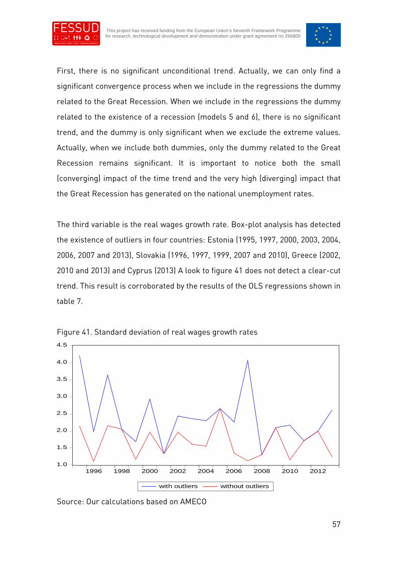
57


First, there is no significant unconditional trend. Actually, we can only find a

significant convergence process when we include in the regressions the dummy

related to the Great Recession. When we include in the regressions the dummy

related to the existence of a recession (models 5 and 6), there is no significant

trend, and the dummy is only significant when we exclude the extreme values.

Actually, when we include both dummies, only the dummy related to the Great

Recession remains significant. It is important to notice both the small

(converging) impact of the time trend and the very high (diverging) impact that

the Great Recession has generated on the national unemployment rates.

The third variable is the real wages growth rate. Box-plot analysis has detected

the existence of outliers in four countries: Estonia (1995, 1997, 2000, 2003, 2004,

2006, 2007 and 2013), Slovakia (1996, 1997, 1999, 2007 and 2010), Greece (2002,

2010 and 2013) and Cyprus (2013) A look to figure 41 does not detect a clear-cut

trend. This result is corroborated by the results of the OLS regressions shown in

table 7.

Figure 41. Standard deviation of real wages growth rates

1.0

1.5

2.0

2.5

3.0

3.5

4.0

4.5

1996 1998 2000 2002 2004 2006 2008 2010 2012



58


Table 7. OLS regression of the standard deviation of real wages growth ratesModel 1

WithOutliers


Model 3With

Outliers


Model 5With

Outliers


Model 7Model With

Outliers


C 2.775(0.000)

1.730(0.000)

2.769(0.000)

1.765(0.000)

2.672(0.000)

1.789(0.000)

1.921(0.000)

1.740(0.000)

Trend -0.040(0.243)

-0.008(0.562)

-0.039(0.474)

-0.014(0.520)

-0.046(0.198)

-0.018(0.118)

0.049(0.183)

-0.012(0.542)

Dcrisis -0.020(0.995)

0.106(0.706)

-1.492(0.024)

-0.113(0.768)


0.135(0.351)

0.795(0.046)

0.198(0.454)

AR(1) -0.432(0.081)

-0.434(0.093)

-0.536(0.047)

-0.571(0.011)

-0.538(0.055)

AR(2) -0.443(0.095)

-0.457(0.097)


(0.243)1.825

(0.195)0.687

(0.517)1.196

(0.346)1.092

(0.359)2.066

(0.148)2.615

(0.048)1.545

(0.253)D-W 2.561 2.169 2.565 2.149 2.572 2.162 2.210 2.184Jarque-Bera 1.411

(0.493)0.825

(0.661)1.381

(0.501)1.393

(0.498)2.375

(0.304)3.899

(0.142)3.845

(0.146)2.476


(0.262)0.004

(0.941)1.094

(0.358)0.699

(0.512)0.372

(0.695)1.171

(0.338)0.833

(0.497)1.108


(0.275)1.741

(0.213)1.455

(0.270)1.948

(0.185)1.185

(0.334)0.053

(0.948)0.202

(0.819)0.213


59


60


We have not detected any conditional or unconditional trend. Moreover, the

dummy variables related to the existence of recession and the Great Recessions

are significant when we include all the data, but they are not longer significant.

In any case it is important to notice that while the existence of a recession leads

to a higher divergence in the unemployment rate in the Eurozone, the Great

Recession has implied a higher convergence in the national unemployment rates.

The fourth variables related to the labour market performance is the real unit

labour costs (ULCs) growth rate. Box-plot analysis have allowed the detection of

a high number of extreme values: Slovakia (1995 and 1996), Estonia (1996, 2007,

2008, 2010 and 2011), Italy (1998), Luxembourg (2001, 2003, 2006, and 2008),

Malta (2001), Greece (2002 and 2013), Cyprus (2002 and 2013) and Ireland (2002,

2004, 2007, 2008 and 2011).

Figure 42. Standard deviation of real unit labour costs growth rates

0.5

1.0

1.5

2.0

2.5

3.0

3.5

1996 1998 2000 2002 2004 2006 2008 2010 2012



61


Table 8. OLS regression of the standard deviation of real unit labour costs growth ratesModel 1

WithOutliers

Model 2Without

Outliers #

Model 3With

Outliers #

Model 4Without

Outliers #

Model 5With

Outliers

Model 6Without

Outliers #

Model 7Model With

Outliers


C 1.791(0.000)

1.159(0.000)

1.661(0.000)

1.301(0.000)

1.795(0.000)

1.143(0.000)

1.479(0.000)

1.535(0.000)

Trend 0.014(0.512)

0.022(0.287)

0.039(0.431)

-0.003(0.887)

0.015(0.529)

0.019(0.353)

0.055(0.198)

-0.024(0.340)

Dcrisis -0.362(0.529)

0.394(0.250)

-0.741(0.252)

0.849(0.064)

Drecession -0.023(0.926)

0.106(0.592)

0.306(0.415)

-0.327(0.261)

AR(1) -0.524(0.085)


(0.512)1.464

(0.243)0.607

(0.557)1.404

(0.276)0.214

(0.809)0.821

(0.458)0.621

(0.612)1.484

(0.267)Wald F-statistics 1.212

(0.287)0.398

(0.678)0.951

(0.408)0.578

(0.572)D-W 1.724 2.368 1.595 2.467 1.722 2.309 1.535 2.094Jarque-Bera 9.819

(0.007)1.229

(0.540)2.489

(0.288)1.199

(0.548)8.817

(0.012)1.341

(0.511)3.111

(0.211)0.726


(0.550)5.734

(0.029)3.051

(0.077)4.416

(0.031)1.420

(0.272)4.075

(0.038)2.303

(0.121)0.998


(0.677)0.679

(0.522)0.532

(0.599)1.181

(0.337)0.377

(0.692)0.625

(0.550)0.661

(0.533)2.441


62


At a glance, it is difficult to find in the figure 42 any clear-cut trend in the evolution

of the standard deviations of real ULCs. Actually, this result is corroborated in

the OLS regressions (see table 8).

We have not been able to detect any significant trend in the evolution of the real

ULCs. Furthermore, the only variable that is statistically significant is the dummy

related to the current economic and financial crisis, which is leading to a higher

divergence in the evolution of the real ULCs. Nonetheless, this result is reached

only when we exclude of the analysis the extreme values.

We want also to emphasize that, contrary to other variables, the explanatory

capacity of the model, measured by the R-squared is very low. This implies that,

besides the non-existence of a trend in the evolution of real ULCs, the evolution

of the dispersion of national ULCs is explained by other variables different than

the very evolution of the business cycle in the Eurozone or the burst of the Great

Recession

Figure 43. Standard deviation of the adjusted wage share

3.0

3.5

4.0

4.5

5.0

5.5

6.0

1996 1998 2000 2002 2004 2006 2008 2010 2012



63


Table 9. OLS regression of the standard deviation of the adjusted wage shareModel 1

WithOutliers


Model 3With

Outliers


Model 5With

Outliers


Model 7Model With

Outliers


C 5.172(0.000)

5.014(0.000)

5.089(0.000)

5.217(0.000)

5.179(0.000)

5.070(0.000)

5.088(0.000)

5.180(0.000)

Trend -0.030(0.273)

-0.030(0.687)

-0.011(0.704)

-0.062(0.479)

-0.028(0.335)

-0.043(0.550)

-0.011(0.720)

-0.059(0.513)

Dcrisis -0.341(0.109)

0.353(0.639)

-0.344(0.161)

0.234(0.802)


-0.175(0.630)

0.003(0.974)

0.118(0.795)

AR(1) 1.208(0.000)

0.630(0.012)

1.324(0.000)

0.582(0.037)

1.228(0.000)

0.596(0.022)

1.324(0.000)

0.577(0.047)

AR(2) -0.659(0.013)

-0.739(0.005)

-0.673(0.015)

-0.739(0.008)


(0.000)5.793

(0.013)10.564(0.000)

3.735(0.036)

8.405(0.001)

3.736(0.036)

7.748(0.002)

2.633(0.082)

D-W 2.330 1.911 1.855 1.966 2.262 1.993 1.855 2.002Jarque-Bera 1.142

(0.564)3.181

(0.203)0.291

(0.864)2.638

(0.267)0.868

(0.647)2.962

(0.227)0.287

(0.866)2.756


(0.380)0.532

(0.476)0.147

(0.863)1.157

(0.340)1.821

(0.198)0.715

(0.505)0.093

(0.962)0.736


0.3861.582

(0.242)0.071

(0.931)1.849

(0.199=0.601

(0.566)2.044

(0.172)0.067

(0.935)2.012


# White Heteroskedasticity-consistent standard errors and covariance

64


The third category of analyzed variables is related to the income distribution in

euro countries. We have analyzed two variables, one related to the income

functional distribution (the adjusted wage share) and the other to the personal

income distribution (the Gini coefficient). In the case of the functional income

distribution, there is only one country that registers extreme values: Slovakia

(1995, 2005, 2007, 2008 and 2009). A look to figure 43 does not allow to detect a

clear-cut trend, and, actually, this preliminary conclusion is corroborated in the

regressions shown in table 9.

We have not found any trend in the evolution of the standard deviation of the

adjusted wage share. Actually, neither the trend nor the two dummy variables

related to the existence of recessions and the Great Recession exert a significant

impact on the dispersion of adjusted wage shares in the Eurozone.

In the case of the dispersion in the personal income distribution, we have not

found any extreme values or outliers. Figure 44 allows to detecting a declining

trend in the dispersion of the Gini coefficient

Figure 44. Standard deviation of the Gini coefficient

2.8

3.2

3.6

4.0

4.4

4.8

5.2

1996 1998 2000 2002 2004 2006 2008 2010 2012


65


The regressions that we have run confirm this idea, detecting a convergence

process in the Gini coefficient (see table 10). The Great Recession would have not

exerted any significant impact. However, the recessions would have a significant

effect, accelerating the process of convergence.

Table 10. OLS regression of the standard deviation of the Gini coefficientModel 1 # Model 2 Model 3 Model 4

C 4.322(0.000)

4.224(0.000)

4.451(0.000)

4.652(0.000)

Trend -0.053(0.037)

-0.032(0.309)

-0.046(0.025)

-0.071(0.059)

Dcrisis -0.338(0.391)

0.469(0.407)


-0.614(0.073)

Mean dependent variable 3.842 3.842 3.842 3.842R2 0.297 0.330 0.437 0.463F-statistic 7.213

(0.015)3.947

(0.040)6.214

(0.010)4.314


(0.036)D-W 1.480 1.591 1.454 1.346Jarque-Bera 0.289

(0.865)0.127

(0.938)0.295

(0.862)0.373


(0.052)1.901

(0.181)1.282

(0.304)1.346


(0.925)0.026

(0.974)0.298

(0.746)0.829


We have also analyzed the existence of a trend in the evolution of national rates

of inflation, measured by the national consumer price indexes (CPI). In this case,

we have found extreme values for 5 countries: Estonia (1995 to 1998, 2007, 2008,

2011 and 2012), Slovenia (1995 to 2000), Slovakia (1998 to 2004, and 2012), Ireland

(2007, 2009, 2010) and Greece (2010, 2012 and 2013). Figure 45 shows the

evolution of the standard deviation of national CPIs with and without these

outliers.

66


Figure 45. Standard deviation of the CPIs


Table 11 confirms the existence of an unconditional convergence process,

regardless the inclusion or exclusion of the outliers. This convergence process

is maintained when we make the analysis of the conditional sigma-convergence.

However, in this case, the impact of the existence of recessions and that of the

Great recession is less obvious.

If we introduce separately both variables, they are significant when we include all

the data (that is when outliers are included), and in both cases the impact is the

same, leading to ha higher divergence in the inflation performance. Excluding

these extreme values, however, implies that they are no longer significant. If we

include simultaneously both variables (models 7 and 8), when outliers are

included no dummy variables is significant. However, the redundant variables

test show that dummy related to the Great Recession is not significant. This

implies that, with and without outliers, only the dummy of the existence of

recessions is significant, and that during recessions there is a higher divergence

in the national inflation rates.

0

1

2

3

4

5

6

7

8

1996 1998 2000 2002 2004 2006 2008 2010 2012


67


Table 11. OLS regression of the standard deviation of the CPIModel 1

WithOutliers #

Model 2Without

Outliers *

Model 3With

Outliers *

Model 4Without

Outliers *

Model 5With

Outliers *


Model 7Model WithOutliers *


C 4.110(0.000)

1.761(0.000)

4.548(0.000)

1.851(0.000)

3.724(0.000)

1.632(0.000)

3.630(0.000)

1.399(0.000)

Trend -0.224(0.004)

-0.077(0.002)

-0.317(0.004)

-0.096(0.010)

-0.246(0.000)

-0.084(0.000)

-0.234(0.009)

-0.055(0.043)

Dcrisis 1.513(0.078)

0.310(0.250)

-0.219(0.852)

-0.542(0.190)


0.408(0.106)

1.318(0.125)

0.648(0.012)


(0.000)23.634(0.000)

17.376(0.000)

12.346(0.000)

24.567(0.000)

19.729(0.000)

15.408(0.000)

14.506(0.000)


13.3190.001)

11.101(0.000)

8.572(0.002)

19.015(0.000)

12.780(0.000)

D-W 0.545 1.064 0.833 1.181 1.189 1.381 1.214 1.551Jarque-Bera 7.311

(0.025)4.818

(0.089)5.099

(0.078)2.271

(0.321)2.322

(0.313)2.233

(0.327)2.065

(0.356)3.777


(0.024)5.235

(0.035)3.348

(0.061)3.371

(0.060)5.222

(0.018)2.359

(0.126)6.083

(0.006)2.350


(0.061)0.377

(0.692)2.390

(0.127)0.267

(0.76891.236

(0.320)0.239

(0.790)1.090

(0.364)1.354

(0.292)p-values in parenthesis# White Heteroskedasticity-consistent standard errors and covariance* HAC standard errors and covariance

68

This project has received funding from the Europeanfor research, technological development and demonstration

In the category of the performance of the national balance of payments, we have

analyzed the dispersion of the balance on current transactions (measured as a

percentage of the GDP). The box-plot analysis has only detected two countries

with extreme values: Luxembourg (1995 and 2000) and Greece (2011). Looking at

the evolution of the standard deviations of this balance (see figure 46), it is

difficult to reach any clear-cur conclusion about the existence of a time trend.

Figure 46. Standard deviation of the balance on current transactions


The regression analysis has detected the existence of a conditional divergence

process that is independent on the inclusion or exclusion of the extreme values

(see table 12). The existence of a recession in the Eurozone is not significant.

However, the Great Recession has generated a high and significant impact,

leading to a strong convergence process in the national balances on current

transactions.

3

4

5

6

7

8

9

1996 1998 2000 2002 2004 2006 2008 2010 2012


69


Table 12. OLS regression of the standard deviation of the balance on current transactionsModel 1

With Outliers*

Model 2Without

Outliers *


#

Model 4Without

Outliers #


#



Model 8Without

Outliers #C 6.172

(0.000)5.933

(0.000)5.406

(0.000)5.084

(0.000)8.887

(0.044)9.730

(0.125)5.448

(0.000)5.098

(0.000)Trend -0.036

(0.462)-0.024(0.755)

0.125(0.011)

0.155(0.006)

-0.244(0.336)

-0.301(0.424)

0.121(0.082)

0.154(0.025)

Dcrisis -2.645(0.003)

-2.931(0.003)

-2.566(0.037)

-2.906(0.022)


-0.302(0.532)

-0.060(0.903)

-0.019(0.967)

AR(1) 0.796(0.001)

0.797(0.001)


(0.462)0.217

(0.646)7.428

(0.005)8.018

(0.007)6.339

(0.006)7.452

(0.003)4.648

(0.017)5.012


(0.754)6.278

(0.009)6.647

(0.007)0.935

(0.415)4.452

(0.019)4.257

(0.023)D-W 0.550 0.496 1.230 1.224 2.202 1.906 1.219 1.221Jarque-Bera 0.174

(0.916)0.233

(0.889)0.165

(0.920)0.625

(0.731)0.665

(0.718)0.254

(0.880)0.173

(0.916)0.632


(0.028)5.433

(0.032)6.320

(0.009)10.037(0.001)

2.886(0.087)

0.211(0.811)

3.921(0.029)

6.243(0.005)


7.635(0.005)

0.837(0.453)

0.786(0.474)

0.202(0.819)

0.272(0.766)

0.812(0.465)

0.755(0.489)

p-values in parenthesis# White Heteroskedasticity-consistent standard errors and covariance* HAC standard errors and covariance

70


The final category analyzed is related to the performance of national public

finances. We have focused our analysis on the evolution of the public budget

balance and the public debt of the general governments, measuring both

variables as percentage of the GDP.

In the case of the public budget balance, the box-plot analysis has detected

extreme values in seven countries: Luxembourg (1997), Greece (2008 and 2013),

Slovenia (2013), Malta (1998), Slovakia (2000) and Ireland (2010 and 2011).

Although the number of outliers is not high, however they lead to relevant

differences in the evolution of the standard deviation of the balance on current

transactions when we exclude these extreme values, as figure 47 shows,

something that could lead to different conclusions depending on the inclusion or

exclusion of these outliers.

Figure 47. Standard deviation of the public budget balance

2

3

4

5

6

7

1996 1998 2000 2002 2004 2006 2008 2010 2012



71


Table 13. OLS regression of the standard deviation of public budget balanceModel 1

WithOutliers


Model 3With

Outliers


Model 5With

Outliers


Model 7Model With

Outliers


C 2.973(0.000)

3.074(0.000)

3.438(0.000)

3.211(0.000)

2.792(0.000)

3.022(0.000)

3.666(0.000)

3.281(0.000)

Trend 0.056(0.172)

-0.005(0.774)

-0.042(0.448)

-0.034(0.250)

0.046(0.258)

-0.008(0.672)

-0.062(0.369)

-0.040(0.279)

Dcrisis 1.605(0.030)

0.471(0.208)

2.037(0.076)

0.603(0.308)


0.166(0.451)

-0.328(0.604)

-0.100(0.765)


(0.172)0.084

(0.774)4.1070.036)

0.903(0.424)

1.931(0.177)

0.339(0.717)

2.708(0.082)

0.598(0.625)

D-W 1.593 1.391 2.209 1.169 1.776 1.225 2.320 1.206Jarque-Bera 26.503

(0.000)1.601

(0.448)16.130(0.000)

0.118(0.942)

23.055(0.000)

0.985(0.610)

14.851(0.000)

0.077(0.961)

Breusch-Pagan-Godfrey 1.192(0.290)

0.104(0.750)

2.123(0.152)

1.670(0.219)

0.761(0.483)

0.410(0.669)

1.495(0.256)

1.378(0.287)


0.936(0.413)

0.358(0.704)

1.440(0.269)

0.348(0.711)

1.303(0.302)

0.576(0.575)

1.158(0.344)


72


As table 13 shows, there is no time trend in the evolution over the years of the

national public budget balances, and consequently we cannot talk of the

existence of a process of conditional or unconditional convergence or divergence

process. It is also important to emphasize that the existence of a recession in the

Eurozone is not significant and that the Great Recession has led to a higher

divergence of national public budgets, although when we exclude the outliers this

variable stops to be significant.

In the case of the public debt, the outliers detected are all of them concentrated

between 1997 and 2002, that is the years before and after the creation of the

European Monetary Union in 1999: Luxembourg (1997, 1998, 1999 and 2000),

Estonia (1997, 1998, 1999 and 2000), Belgium (1997, 1998, 1999, 2000 2001 and

2002), Italy (1997, 1998, 1999 and 2000) and Greece (2000). The large difference

recorded in the evolution of the standard deviation of public debt in these years

makes difficult to find any clear time trend, mainly when all countries and years

are included in the analysis (see figure 48).

Figure 48. Standard deviation of the public debt

10

15

20

25

30

35

40

45

1996 1998 2000 2002 2004 2006 2008 2010 2012



73


Table 14. OLS regression of the standard deviation of public debtModel 1

WithOutliers #

Model 2Without

Outliers #

Model 3With

Outliers #

Model 4Without

Outliers #

Model 5With

Outliers #

Model 6Without

Outliers #


Model 8Without

Outliers #C 3.078

(0.952)21.059(0.000)

31.538(0.000)

22.829(0.000)

27.632(0.000)

19.063(0.000)

30.038(0.000)

16.818(0.002)

Trend 1.899(0.436)

0.878(0.019)

-0.186(0.180)

0.503(0.323)

0.250(0.026)

0.767(0.021)

-0.050(0.766)

1.048(0.025)

Dcrisis 8.438(0.001)

6.114(0.102)

5.606(0.130)

-5.231(0.430)


6.319(0.052)

2.155(0.245)

8.632(0.129)

AR(1) 0.871(0.000)


(0.000)10.534(0.004)

16.631(0.000)

6.096(0.010)

16.664(0.000)

9.427(0.001)

12.242(0.000)

6.267(0.005)


6.648(0.019)

8.864(0.002)

16.247(0.000)

11.132(0.000)

14.603(0.000)

8.068(0.001)

13.736(0.000)

D-W 2.358 0.928 1.113 1.029 1.235 1.619 1.296 1.884Jarque-Bera 1.340

(0.511)0.652

(0.721)0.376

(0.828)0.747

(0.688)1.855

(0.395)1.101

(0.576)1.469

(0.479)1.043


(0.018)9.673

(0.006)6.271

(0.009)6.610

(0.008)2.953

(0.081)7.309

(0.005)3.758

(0.034)6.245


(0.551)1.980

(0.172)1.127

(0.351)1.643

(0.228)0.834

(0.454)0.436

(0.654)0.812

(0.465)1.084


74


Table 14 shows the existence of an unconditional divergence process that takes

place when the outliers are excluded of the analysis (see model 2). This

divergence process accelerates during recessions (models 5 and 6)

4.3 Conclusions

The analysis carried out in the previous section has given rise to different results,

depending on the analyzed variable. In the cases of the adjusted wage share, the

real ULCs growth rate, the real wages growth rate and the public budget balance,

we have not found a significant time trend, and, therefore, we cannot talk of the

existence of a convergence or divergence process.

Only in the cases of the unemployment rate, the Gini coefficient and the inflation

rate there is clear and significant convergence process. On the contrary, in the

cases of the real GDP per capita, the GDP growth rate, the output gap, the balance

on current transactions and the public debt we have detected a significant

divergence process, thus exacerbating the differences existing before the

creation of the European Monetary Union.

If we focus on the dummy variables related to the existence of a recession in the

Eurozone and the current Great Recession, we find again mixed results. Thus,

recessions lead to a divergence in the unemployment rate, the employment

growth rate, the public budget balance and the public debt. Conversely, it

contributes to reduce the national differences in the real GDP per capita and the

balance on current transactions. The Great Recession, on its behalf, is

contributions to a convergence in the real GDP per capita and the balance on

current transactions (like recessions), and to a divergence in the unemployment

rate, the employment growth and the fiscal imbalances.

75


Finally, unclear results have been obtained in some variables like the potential

GDP growth rate, the employment growth and the real GDP growth rate. The

reason is that the results obtained depend on we include or not the extreme

values.

In sum, our analysis has not been able to find a significant convergence in the

macroeconomic performance of EMU countries. On the contrary, our result point

out to a higher divergence in the macroeconomic performance of Eurozone

countries. Moreover, we have found that both recessions and the current crisis

generate a relevant and significant impact on the convergence-divergence

process, implying that the results obtained in previous studies on the

convergence in the Eurozone can be affected by the period analyzed and the

situation of the business cycles in the whole Eurozone and in the member states.

Finally, we want to emphasize that the Great Recession has increased the

divergence in many macroeconomic outcomes, generating the risk of a higher

heterogeneity if the crisis becomes chronic-endemic or makes structural the bad

performance (low growth-stagnation) recorded in many countries.

4. Conclusions

The different descriptive and empirical analyses developed in the deliverable

have shown that the impact of the economic and financial crisis in the European

Union, a shock that can be considered as a common shock for the whole area,

has not been symmetrically distributed and that that impact has been more

intense in euro that in no-euro European Union countries. Moreover, if we focus

our attention on the performance of the Eurozone, it is again clear that within the

euro area, the impact of the crisis has been more severe in the PIIGS countries

(Portugal, Ireland, Italy, Greece and Spain) and in the new member states. In

76


other words, the crisis has been more severe in the peripheral countries that in

the core euro countries.

These results, that is, the facts that, first, the impact of the crisis has been larger

in the Eurozone in relation to other developed and developing economies and

other non-euro EU countries, and, second, that, within the Eurozone the effects

of the crisis have been more severe in the peripheral countries, imply that there

are common (structural problems of competiveness) and individual-endemic

problems (endemic of some economies) affecting the euro countries.

Therefore, the crisis has led to a rising divergence in the euro area, exacerbating

previous differences in the economic performance of euro countries. As far as

this divergence has not only a cyclical nature, but also a structural-permanent

one, the coherence of the Eurozone can diminish, making the working (survival?)

of the (current?) euro area more problematic.

References

Arestis, P. and Sawyer, M. (eds.) (2012) The Euro Crisis, Palgrave Macmillan,

Basingstoke.

Benczes, I. and Szent-Ivanyi (2015) “The European economy in 2014: fragile

recovery and convergence”, Journal of Common Market Studies, 53, S1, pp. 162-

180.

Bitzenis, A., Karagiannisand, N. and Marangos, J. (eds.) (2015) Europe in Crisis.

Problems, Challenges and Alternative Perspectives, Palgrave Macmillan,

Basingstoke.

77


Carrasco, C.A., Ferreiro, J., Gálvez, C., Gómez, C. and González, A. (2016) “The

impact of the financial and economic crisis on European Union Member States”,

in Hein, E., Detzer, D.and Dodig, N. (eds.) Financialisation and the Financial and

Economic Crises. Country Studies, Edward Elgar, Cheltenham , forthcoming.

Carrasco, C.A. and Peinado, P. (2015) “On the origin of European imbalances in

the context of European integration”, Panoeconomicus, 62(2), pp. 177-191.

Cavallo, A. and Ribba, A. (2015) “Common macroeconomic shocks and business

cycle fluctuations in Euro area countries”, International Review of Economics and

Finance, 38, pp 377-392.

Dodig, N. and Herr, H. (2015) “Current account imbalances in the EMU: an

assessment of official policy responses”, Panoeconomicus, 62(2), pp. 193-216.

Ferroni, F. and Klaus, B. (2015) “Euro area business cycles in turbulent times:

convergence or decoupling”, Applied Economics, 47, 34-35, pp. 3791-3815.

Gächter, M. and Riedl, A. (2014) “One money, one cycle? The EMU experience”,

Journal of Macroeconomics, 42, pp. 141-155.

Gibson, H.D., Palivos, T. and Tavlos, G.S. (2014) “The crisis in the Euro area: an

analytical overview”, Journal of Macroeconomics, 39, Part B, pp. 233-239.

Mendonça, A. (2014) “The European crisis and global economy dynamics:

continental enlargement versus Atlantic opening”, Panoeconomicus, 5, Special

Issue, pp. 543-569.

78


Mongelli, F.P. (2013) “The mutating euro area crisis. Is the balance between

“sceptics’’ and “advocates” shifting?” European Central Bank Occasional Paper

Series, No. 144.

Onaran, Ö. (2011) “The crisis in Western and Eastern EU: does the policy reaction

address its origin”, in Arestis, P. Sobreiro, R. and Oreiro, J.L. (eds.) An

Assessment of the Global Impact of the Financial Crisis, pp. 135-158, Palgrave

Macmillan, Basingstoke.

Perraton, J. (2011) “Crisis in the Euro zone”, in Arestis, P. Sobreiro, R. and Oreiro,

J.L. (eds.) An Assessment of the Global Impact of the Financial Crisis, pp. 84-

107, Palgrave Macmillan, Basingstoke.

79


Financialisation, Economy, Society and Sustainable Development (FESSUD) is a

10 million euro project largely funded by a near 8 million euro grant from the

European Commission under Framework Programme 7 (contract number :

266800). The University of Leeds is the lead co-ordinator for the research project

with a budget of over 2 million euros.

THE ABSTRACT OF THE PROJECT IS:

The research programme will integrate diverse levels, methods and disciplinary

traditions with the aim of developing a comprehensive policy agenda for changing

the role of the financial system to help achieve a future which is sustainable in

environmental, social and economic terms. The programme involves an

integrated and balanced consortium involving partners from 14 countries that

has unsurpassed experience of deploying diverse perspectives both within

economics and across disciplines inclusive of economics. The programme is

distinctively pluralistic, and aims to forge alliances across the social sciences, so

as to understand how finance can better serve economic, social and

environmental needs. The central issues addressed are the ways in which the

growth and performance of economies in the last 30 years have been dependent

on the characteristics of the processes of financialisation; how has

financialisation impacted on the achievement of specific economic, social, and

environmental objectives?; the nature of the relationship between

financialisation and the sustainability of the financial system, economic

development and the environment?; the lessons to be drawn from the crisis

about the nature and impacts of financialisation? ; what are the requisites of a

financial system able to support a process of sustainable development, broadly

conceived?’

80


THE PARTNERS IN THE CONSORTIUM ARE:

Participant Number Participant organisation name Country

1 (Coordinator) University of Leeds UK

2 University of Siena Italy

3 School of Oriental and African Studies UK

4 Fondation Nationale des Sciences Politiques France

5 Pour la Solidarite, Brussels Belgium

6 Poznan University of Economics Poland

7 Tallin University of Technology Estonia

8 Berlin School of Economics and Law Germany

9 Centre for Social Studies, University of Coimbra Portugal

10 University of Pannonia, Veszprem Hungary

11 National and Kapodistrian University of Athens Greece

12 Middle East Technical University, Ankara Turkey

13 Lund University Sweden

14 University of Witwatersrand South Africa

15 University of the Basque Country, Bilbao Spain

The views expressed during the execution of the FESSUD project, in whateverform and or by whatever medium, are the sole responsibility of the authors. TheEuropean Union is not liable for any use that may be made of the informationcontained therein.

Published in Leeds, U.K. on behalf of the FESSUD project.

impact of crisis on eu - welcome -...

Documents