impact of electric locomotive traction of the passenger

Mechanics & Industry 18, 222 (2017)c© AFM, EDP Sciences 2017DOI: 10.1051/meca/2016047www.mechanics-industry.org

Mechanics&Industry

Impact of electric locomotive traction of the passenger vehicleRide quality in longitudinal train dynamics in the contextof Indian railways

Sunil Kumar Sharma1,a and Anil Kumar2

1 Centre for Transportation Systems, Indian Institute of Technology Roorkee, India2 Department of Mechanical and Industrial Engineering, Indian Institute of Technology Roorkee, India

Received 9 November 2015, Accepted 12 July 2016

Abstract – Rail transport is one of the major modes of transportation in India. The dynamic performanceof a railway vehicle, in terms of serviceability and safety, was evaluated on the basis of specific performanceindices such as ride quality and comfort. This paper is an attempt to analyse the longitudinal dynamicmodel of the passenger train for the attainment of better vehicle ride quality and comfort. The modellinghas been done in two phases: in the first phase, a mathematical model was analysed which was further usedfor the evaluation of the longitudinal dynamic forces that appear on the buffer, draw gear and fasteningdevices during the braking process. The second phase includes simulation of longitudinal train dynamicsconsidering the effects of forces like rolling resistance, brake force, coupler force and the gravitational forceacting externally on a vehicle for better ride quality and comfort in comparison to the traction effect onWAP-5 and WAP-7 Indian locomotives. The Sperling ride index and ISO 2631 were used respectively tocalculate the ride quality and comfort using filtered RMS accelerations. Simulation results revealed thatWAP-5 was better at an initial speed of 30 km.h−1 and 45 km.h−1, whereas, the WAP-7 gave better ridequality and comfort than WAP-5 at and above the speed of 60 km.h−1.

Key words: Longitudinal vehicle dynamics / traction force / sperling ride index / dynamic behaviour /ride quality / ride comfort

1 Introduction

The efficient working of Indian Railways is dependenton various factors which include safety parameters alongwith the efficiency of its locomotive which is responsiblefor the rapid acceleration of the train, and also its brakingsystem which enables the train to bring it to a standstillat the station, even on an adverse gradient.

Electric engines are the lightweight locomotive vehi-cles that constitute mainly motors and wheel axles. Incomparison to a diesel engine, an electric engine has al-most no moving parts, therefore, electric engines are eas-ier to maintain. Moreover, due to the light weight, theengines resulted in less wear and tear of the railwaytracks [1]. The electric engine draws power from overheadequipment and requires only a transformer and regulatorto convert the power into the operational level. Currently,the electric locomotives used by Indian Railway (IR) forpassenger transports are broad gauge AC traction motive

a Corresponding author: [email protected]

power passenger service locomotives (WAP), i.e. WAP- 4,WAP- 5, WAP- 7 series [1].

IR is contemplating to lay exclusive passenger corri-dors for movement of semi-high speed trains. It is alsoplanned to upgrade the speed of passenger trains upto150 km.h−1 on existing tracks and 200 km.h−1 on pro-posed passenger corridors [2]. For this, Research Designand Standards Organisation (RDSO) conducted a testtrail with 24-coach 1430 tonne passenger rake for acceler-ation and deceleration rate [1]. The trail concluded thatWAP-7 can accelerate faster than the WAP-5, but the ve-hicle ride quality was not observed. This led to the emer-gence of a specific issue, i.e. which locomotive providesbetter stability and comfort at various speeds. Thus, theride stability and comfort becomes a topic to identify theride quality and comfort at various speed. This analy-sis examines the comfort level of passengers caused dueto changes in the movement of a vehicle’s longitudinaldirection, viz. travelling direction. Per contra, the limita-tion while operating a vehicle network at high velocity,high capacity and short trip times might affect passenger

Article published by EDP Sciences

https://doi.org/10.1051/meca/2016047

http://www.mechanics-industry.org

http://www.edpsciences.org

S.K. Sharma and A. Kumar: Mechanics & Industry 18, 222 (2017)

Table 1. Details of the two electric locomotives [1,3,4].

Electric locomotive WAP-5 WAP-7Traction Mo-tors(TM)

ABB’s 6FXA 7059 3-phase squirrel cageinduction motors (1,583/3,147 rpm,2,180 V, 1,150 kW, 370/450 A). Torque6,930/10,000 Nm, partially suspended,Forced-air ventilation, Weight 2,050 kg,96% efficiency

6FRA 6068 3-phase squirrel-cage induc-tion motors (2,180 V, 850 kW, 1,283/2,484rpm, 270/310 A). Torque 6,330–7,140 Nm,nose suspended, axle-hung, forced air ven-tilation, Weight- 2,100 kg, 95% efficiency

Gear Ratio 67:35:17 72:20Axle load (tons) 19.5 t 20.5 tPower Max: 6,000 hp (4,474kW) Max: 6,350 hp (4,740 kW)Tractive effort Max: 258 kN Max: 323 kNWheel diameter New: 1,092 mm, Full-worn: 1,016 mm New: 1,092 mm, Full worn: 1,016 mmBogies Bo-Bo, Henschel Flexifloat Co-Co, Fabricated Flexicoil Mark IVlocomotive weight(tons)

78 t 123 t

Braking Air Braking Air BrakingTrain coupling Central Buffer Couplers Central Buffer Couplers

intolerance due to high longitudinal acceleration. Thus,it implies that the tolerance limit of passengers towardsthe longitudinal acceleration will have an impact on thedesign of the vehicle braking and traction system.

In this paper, a comparative study of WAP -5 andWAP-7 electric locomotives considering a double deckertrain of 14 coaches using a universal mechanism (UM) onMumbai-Ahmedabad rail route in India is presented. Inthis analysis, calculation of the acceleration of train inthe longitudinal direction is done while keeping all otherparameters constant. Moreover, the ride quality and com-fort were evaluated using the Sperling ride index and ISO2631-1997, respectively. For this analysis, different initialspeeds, i.e. 30, 45, 60, 90, 120, 150 and 180 km.h−1 weretaken into consideration. The details of the locomotiveswere given in Table 1.

2 Mathematical modelling of longitudinaltrain dynamics (LTD)

2.1 Longitudinal model of the train

A coach running on track was subjected to the fol-lowing types of forces which exert longitudinally in thetrain. Figure 1 shows the model of a train as a cascadecomposition of mass points in the longitudinal direction.

The mechanical behaviour of the vehicle was simulatedaccording to a quite efficient mono-dimensional model ofthe train which was developed in prior researches [5–7]and is explained by Equation (1) that characterizes themotion of the vehicle as Newton’s second law of motion:where for the ith vehicle the force relationship is devel-oped. xi = the longitudinal displacement of the ith vehi-cle and xi−1, xi+1 = longitudinal displacement of the foreand aft vehicle, respectively.

mixi = ±Fcw(lead)i±Fcw(trl)i

−Fbrki±Ft/db±Fgradi−Frri

(1)

On each vehicle mass (mi) which forms the train at aspeed of v, the following forces act: inertial force, brak-ing force Fbrki , resistance to motion Frri , grade resis-tance Fgradi , traction or braking effort Ft/db and finallythe force from the buffer and draw gear device, i.e. cou-pler force from leading coach Fcw(lead)i

and trailing coachFcw(trl)i

.The solution to the Equation (1) describes that the

movement of vehicles during emergency braking is ob-tained by numerical integration using an original calcula-tor program elaborated in MATLAB [8] for a time periodof t = 10 s. Thus, determination of the state variablesof the system, i.e. the the displacement and the relativevelocity between vehicles can be done. Further, the forcesdeveloped in the buffers and traction devices can be cal-culated. For this purpose, it is necessary to first calculatethe resistances to the motion and braking forces.

Taking into consideration the vehicle ith, the resis-tance to motion is determined by the formula in Equa-tion (2) [9, 10].

Frri = migrvi (2)

where, rvi represents the specific resistance to motion ofthe ith vehicle and g gravitational acceleration. It shouldbe specified that the resistance to motion is a character-istic specific for each type of vehicle, which is calculatedusing empirical formulas, as follows in Equation (3) [11].

rvi = f (v) (3)

Locomotive (WAP 7): 0.754 + 0.00933v + 0.00002641v2

Locomotive (WAP 5): 1.34819 + .02153v + 0.00008358v2

Passenger (LHB): 1.43 + 0.0054v + 0.000253v2

As for the braking force, the vehicle was equipped withaxle mounted disc brakes in order to have an effectivebrake power to halt the train within the emergency brak-ing distance. The brake forces were acted on the discsfitted on the axles. Therefore, the braking force is calcu-lated using Equation (4) [10].

18-page 2


Fig. 1. Longitudinal model of the train [5,6].

Table 2. Brake modelling parameter.

Parameter Description

dbc Brake cylinder diameter (254.8 mm)

FsR Release spring force (1.3 kN )

Do Wheel diameter (1092 mm)

rm Medium friction radius (588 mm)

nbc Number of brake cylinders of the vehicle (i.e. locomotive (8) and coaches (2))

μd The friction coefficient between discs and pads (0.35)

ηbr Mechanical efficiency of the brake rigging (95%)

it Amplification ratio (1.954)

The air brake force

Fbrk(i) =((

πd2bc

4

)ηcylpmax(i) − FsR

)itnbc

2rm

D0μdηbr

(4)Brake modeling parameters is listed in Table 2.

Finally, The couplers used on LHB coaches are tightlock center buffer couplers of AAR type H [12]. The con-nection between two contiguous coaches within a trainis maintained by a “Coupler System” which consists ofa tight lock coupler head (AAR type H) with drawbar,drawbar guide (support) and draft gear (draw and buffinggear). The draft gear plays a very crucial role by absorbingthe superfluous energy in both draw and buff mode. Thedraft gear consists of elastic elements and friction springs,thus are able to transmit both the tensile and compres-sive forces. The modelling for coupler system consistingelastic and friction element in the buffer and draw gearhas also been studied by Craciun and Mazilu [9].

Hence, mathematical modelling for draft gear ismainly aimed to establish a relation between the couplerforces and its relative displacement, in the course of trainbraking. These forces depend on the variation of relativedisplacement and relative velocity due to the rigidity ofelastic elements, as well as the damping degree. In undermentioned Equation (5), ka is a constant which dependson upon the elasticity of the material and kfr which isa frictional spring constant, i.e. a function of the frictionbetween the inner and outer rings [12, 13]. Moreover,the coupler system consists of a tight lock at the couplerhead and it is subjected to a preload for holding the ad-jacent coupler head which is here denoted by P . Thus,

the following Equation (5) is used to evaluate the couplerforces (5).

Fcw(x, x) =

⎧⎨⎩

kabx + kfrb |xi| tanh (u.x) + P for x < 0,P for x = 0,kadx + kfrd |xi| tanh (u.x) + P for x > 0

(5)In Equation (5), the relative displacement of the strokein the draft gear is represented as x and x its relativevelocity. This Equation (5) is used to compute the char-acteristics of the draft gear as shown in Figure 2. If therelative displacement, x < 0 the coupler assembly is incompression (buff), whereas if the relative displacement,x = 0 then the coupler assembly is in preload tensilecondition. Likewise, if the relative displacement is greaterthan 0 (x > 0), the coupler assembly is in tensile mode(draw gear).

For performing simulation, the main parameters usedfor buffers are P = 25 kN, kab = 11 785 kN.m−1, kfrb =5457 kN.m−1 and for draw gear kad = 9430 kN.m−1,kfrd = 4365 kN.m−1. To maintain the standard, themodel must meet the following characteristics: the staticimpedance should be ≤ 1600 kN (maximum), capacity≤35 kJ and the damping factor ought to be ≥60% [13].The respective coupler forces yielded the static impedanceforce of the buff and draw gear as shown in Figures 2aand 2b.

Following is the outcome as given in Table 3 of variousinitial velocities taken into consideration under buff anddraw gear mode.

18-page 3


-0.10 -0.08 -0.06 -0.04 -0.02 0.00 0.02 0.04 0.06 0.08 0.10

-1

0

1

Cou

pler

for

ce (

MN

)

R elative dis placement (m)

B uff

Draw gear

2 m/s1 m/s

0.5 m/s

(a)

(a)

0.0 0.2 0.4 0.6 0.8 1.0 1.2 1.4 1.6

-1

0

1

(b)

0.5 m/s Draw gear 0.5 m/s B uff 1.0 m/s Draw gear 1.0 m/s B uff

2.0 m/s Draw gear 2.0 m/s B uff

Cou

pler

for

ce (

MN

)

T ime (s)

(b)

Fig. 2. (a) Force-displacement characteristic of the coupler. (b) Buffer and draw gear force time history for 0.5,1.0 and 1.5 m.s−1

initial velocity.

Table 3. Effect of initial velocity in the coupler force and displacement.

Initial velocity (m.s−1) Mode Displacement (m) Coupler Force (kN)

0.5Buff 0.020 283.6

Draw gear 0.015 271.2

1Buff 0.041 567.1

Draw gear 0.031 542.6

2Buff 0.081 1134.5

Draw gear 0.060 1085.2

2.2 Traction modules

Tractive effort (TE) is the force generated by a loco-motive in order to generate motion through tractive forceand braking effort (BE). It is a measure of the brakingpower of a vehicle. Nevertheless, the behaviour of locomo-tives was independent and it was necessary to control thatkind of behaviour in relation to speed, time, and position.TE and BE were evaluated experimentally by RDSO [14]as shown in Figures 3a and 3b and the same were taken forthe analysis in Universal Mechanism. Thus, to have ver-satility in the module, the force gradient during tractionimplementation and removal could also be coerced andlastly, the entire power was exposed to the linear varia-tion from zero to maximum power [6]. Moreover, TE/BEalso depends on various factors which include horsepowerof the electric engine, the ability of the main generator,the ability of traction motors, gear ratio and adhesion(weight on driving wheels, rail condition, wheel slip con-trol system, and inverter system).

2.3 Autocorrelation coefficient function

The autocorrelation coefficient function is a mathe-matical phenomenon which is considered for evaluatingthe randomness of the signal. Randomness is calculatedby computing autocorrelation for data values at differ-ent time lags. Its value (results) predict randomness,then in such case, the value of autocorrelation must beclose to zero for each and every time-lag separations. Ifit is non-random, then the value of its autocorrelationswould be significant at non-zero. However, for a signalf(t) as our random forcing function, along the time axis,an average value of the product f(t)f(t + τ) is given

by Equation (6) [15].

Rff (τ) = limx→∞

1T

∫ T

−T2

f (t)f (t + τ ) dt (6)

From the above-mentioned Equation (6), the quantityRff (τ) is always a real-valued even function with amaximum occurring at τ = 0, was a so-called randomauto-correlation function. In physical terms, the autocor-relation function gives the relationship which explains thedependency of a particular instantaneous amplitude valueof the random time signal on the previous occurring am-plitude value. A random process is said to have an ideal-istic condition, the autocorrelation function comprises ofa δ function at τ = 0. The new function, Rff (τ), which iseven, real-valued, goes to zero as τ becomes large (bothpositively and negatively) and obeys the Dirichlet condi-tion given in Equations (7) and (8) [16].

Rf (∞) =[f (t)

]2 (7)

f (t) =√

Rf (∞) (8)

The mean value of f(t) is equal to the positive squareroot of the autocorrelation as the time displacement be-comes very long. Autocorrelation plots were obtained byvertical axis: autocorrelation coefficient is given by Equa-tion (9) [15].

Rh = ch/c0 (9)

ch =1N

N−h∑t−1

(ft − f

) (ft+h − f

)(10)

c0 =∑N

t=1

(ft − f

)2/N (11)

where c0 is variance function, Rh was between –1 and +1and N is the sample size and on the horizontal axis, there

18-page 4


30 60 90 120 150 180

-150

-100

-50

0

50

100

150

200

250

B raking effort

TE/

BE

(kN

)

S peed (km/h)

Tractive effort

(a)(a)

30 60 90 120 150 180

-200

-100

0

100

200

300

(b)B raking effort

Tractive effort

TE/

BE

(kN

)

S peed (km/h)

(b)

Fig. 3. (a), (b): TE/BE v/s Speed forWAP-5, WAP-7 locomotive respectively [14].

Table 4. Ride quality evaluation scales [17].

Ride quality Ride index (Wz)Dangerous 5

Not acceptable for running 4.5Acceptable for running 4

Satisfactory 3Good 2

Very good 1

will be time lag (h = 1, 2, 3 . . .) and ch is auto covariancefunction.

2.4 Sperling ride quality index

Sperling proposed a ride index and developed the so-called Wz method (Werzungzahl). Wz was the frequencyweighted r.m.s value of the different accelerations evalu-ated over defined time intervals or over a defined tracksection. For an arbitrary acceleration signal, which wasnot necessarily a harmonic signal, the frequency-weightedroot mean square value of accelerations (awrms) should beused. The original mathematical expression, introducedby Sperling is given in Equation (12) [17].

Wz = 4.42 (awrms)3/10 (12)

The rail vehicle was accessed on Sperling’s ride evaluationscales mentioned in Table 4, in order to judge the ridequality.

2.5 ISO 2631:1997 for Ride comfort

ISO 2631 provides basic and additional evaluationmethod based on the crest factor. Moreover, ISO 2631-1 Section 6 specifies an r.m.s. based method for evalua-tion of ride comfort [18]. The weighted r.m.s. acceleration

(aw(t) in m.s−2) of a discrete time-domain signal is givenin Equation (13).

aw =

⎡⎣ 1

T

T∫0

a2w (t) dt

⎤⎦

12

(13)

The standard defines the total vibration value of weightedr.m.s. acceleration for all directions in the respective po-sition. At present, however, in that analysis only the lon-gitudinal direction was considered. As per ISO-2631, Ta-ble 5 gives approximate indications of likely reactions tovarious magnitudes of overall vibration values in publictransport.

3 Multibody modeling of WAP-5 and WAP-7for LTD

LTD modelling was done by considering no effectof the vertical or the lateral movement of the vehicle.Based on these assumptions, the forces which were takeninto consideration in the train includes traction forces,air brake forces, in-train forces (coupler forces), dynamicbrake forces, gravitational component, curving resistanceand propulsion resistance. However, in the modelling ofthe passenger train connection systems air brake forcesand in-train forces were probably the two most difficulttask in LTD simulations [5].

3.1 Train modelling

The train model consists of a locomotive, i.e. WAP-7 and WAP-5, double-decker coaches, generator/luggagevan and in train connection called AAR “H”’ Type Tight

18-page 5


Table 5. Ride comfort measure for r.m.s acceleration measuring level.

Perception r.m.s acceleration vibration level

Extremely uncomfortable Greater than 2 m.s−2

Very uncomfortable 1.25 m.s−2to 2.5 m.s−2

Uncomfortable 0.8 m.s−2to 1.6 m.s−2

Fairly uncomfortable 0.5 m.s−2to 1 m.s−2

A little uncomfortable 0.315 m.s−2to 0.63 m.s−2

Comfortable Less than 0.315m.s−2

Fig. 4. Positions of cars in train model.

Lock couplers having balanced type draft gear. Moreover,the train involves a total of 14 coaches and a locomotive.The configuration for both the train with the position oflocomotive and coaches are shown in Figure 4. Where Lstands for the locomotive, C1-C12 are AC double deckerchair car and EOG is generator/luggage van. However,the parameters of train, i.e. code and weight were givenin Table 6 [19].

3.2 Track conditions

In this analysis, a track between Mumbai to Ahmed-abad of Indian Railway was selected. The track length isabout 492.7 km long, and has a maximum grade of twopercent. The track is very straight hence the track cur-vature does not have much influence in the analysis. Thetrack elevation is shown in Figure 5 [19].

3.3 An overview of the Universal Mechanism Tool

In this paper, a program package “Universal Mecha-nism” was utilised to carry out the analysis, which was de-signed to automate the analysis of mechanical objects andrepresented as a multibody system (MBS) [20]. Withinsuch systems, bodies represented as rigid objects werelinked by means of kinematic and force elements. The uni-versal mechanism was facilitated with friendly user inter-face modelling and analysis. The locomotives and coachesin the model were arranged according to train configura-tion shown in Figure 4. The train configured as WAP-7locomotive having Co-Co, Fabricated Flexicoil Mark IVbogies, Double decker coaches, and generator/luggage vanwere shown in Figure 6a and another train which involvesWAP-5 locomotive having Bo-Bo, Henschel Flexifloat bo-gie was shown in Figure 6b.

In the universal mechanism, the PARK solver wasused for the simulation of the longitudinal train vehicledynamics. Moreover, the selection of the solver was madeby comparing rational parameters of different solvers. The

error tolerance in the case of Park solver is 4E-6 to 1E-7 and the time step size was 0.02 s. Moreover, it wasrecommended to set zero value for the minimal step sizefor accurate analysis, but it increases the computationalcost [21]. PARK was an implicit solver of the second orderwith a variable step size which was much more efficientboth for ODE and DAE than another solver [21].

3.4 Model validation

To validate the locomotive model an experimental casestudy was taken into consideration which was tested byRDSO. In that experiment, a test trail was conductedwith 24-coach 1430 tonne passenger rake for accelerationand deceleration rate [1].

The trail concluded that WAP-7 could acceleratequicker than WAP-5. If the WAP-7 was operated on a25 km route then it would be able to attain the speed of0–110 km.h−1 in 240.1 s as compared to 312.1 s of WAP-5.Also, WAP-7 reaches 120–130 km.h−1 in 393.8 s as com-pared to WAP-5 which achieves that speed in 556.2 s asshown in Table 7 [1].

On the other hand, WAP-7 takes 200 s to reach 0–110 km.h−1 and 333.32 s to reach 0–130 km.h−1 as com-pared to WAP-5 which took 287.9 s and 535.2 s respec-tively using Universal Mechanism. The difference in theobservations of the simulation analysis was primarily at-tributable to the consideration of various factors in thex-axis only, whereas in the experimental analysis factorssuch as track irregularity, suspension forces, etc. were con-sidered in all the direction. That led to an emergence of anopportunity for the LTD simulations which could be val-idated through comparative studies by keeping the sameconditions as RDSO has kept in its test trail. The re-sult showed that there was a good agreement between themeasured data and the simulated results. Moreover, foracceleration validation, the numerical simulation is com-pared with the simulation from the Universal Mechanism.The train model with loco +2 coaches is taken for theanalysis. The distribution of acceleration developed in the

18-page 6


Table 6. Types of Coaches and their respective weight [12].

Sr.no Type of Coach and Locomotive CodeWeight in tonsTare Gross

1. WAP-7 WAP-7-LOCO 1232. WAP-5 WAP-5-LOCO 783. Generator cum Luggage van(EOG) LWLRRM 52.12 56.784. Ac double decker chair car (C) ACCC DOUBLE DECKER 45.5 65

0 100 200 300 400 5000

20

40

60

Tra

ck e

leva

tion

(m

)

Dis tance (km)

Fig. 5. Track elevation of Mumbai to Ahmedabad [19].

(a)

(b)

Fig. 6. (a) Model of train 1: WAP-5, double decker and Generator/language van. (b) Model of train 2: WAP-7, double deckerand Generator/language van.

Table 7. Accelerate comparison of the WAP-7 and WAP-5.

Locomotive 0–110 km.h−1 Time (s) 0–110 km.h−1 Time (s) 0–130 km.h−1 Time (s) 0–130 km.h−1 Time (s)experimentally [1] simulation experimentally [1] simulation

WAP-7 312.1 200 393.8 333.32WAP-5 240.1 287.9 556.2 535.2

18-page 7


0 2 4 6 8 10-2

-1

0

1

2

Ac

cel

erat

ion

(m/s

2 )

T ime (s)

Locomotive WAP-5(Univers al mechanism) Locomotive WAP-5(Numerical s imulation) C oach 1-E OG(Univers al mechanism) C oach 1-E OG(Numerical mechanism) C oach 1-C C (Univers al mechanism) C oach 1-C C (Numerical mechanism)

(a)

(a)

0 2 4 6 8 10-2

-1

0

1

2

Ac

cel

erat

ion

(m/s

2 )

T ime (s)

L ocomotive WAP-7(Univers al mechanism) L ocomotive WAP-7(Numerical s imulation)

C oach 1-E OG(Univers al mechanism) C oach 1-E OG(Numerical mechanism)

C oach 1-C C (Univers al mechanism) C oach 1-C C (Numerical mechanism)

(b)

(b)

Fig. 7. Train model hauled by (a) WAP-5 (b) WAP-7.

train body is found via the braking process. In the anal-ysis, to evaluate the acceleration, the train model whichcomprises of a locomotive and 2 coaches were consideredunder the effect of emergency braking at the initial speedof 150 km.h−1 as shown in Figure 1. The result based onnumerical simulation is evaluated using MATLAB. More-over, the measured acceleration from the numerical sim-ulation is compared with the result obtained from the

software for both the trains, i.e. Train 1 hauled by WAP-5 and Train 2 hauled by WAP-7 as shown in Figures 7aand 7b.

The vehicle accelerations from the Universal Mecha-nism and numerical simulation showed a good agreementand were within allowable ranges. The slight variation isdue to the gradient resistance force. In Indian railway,the criterion for the in-train forces of the coupler is not

18-page 8


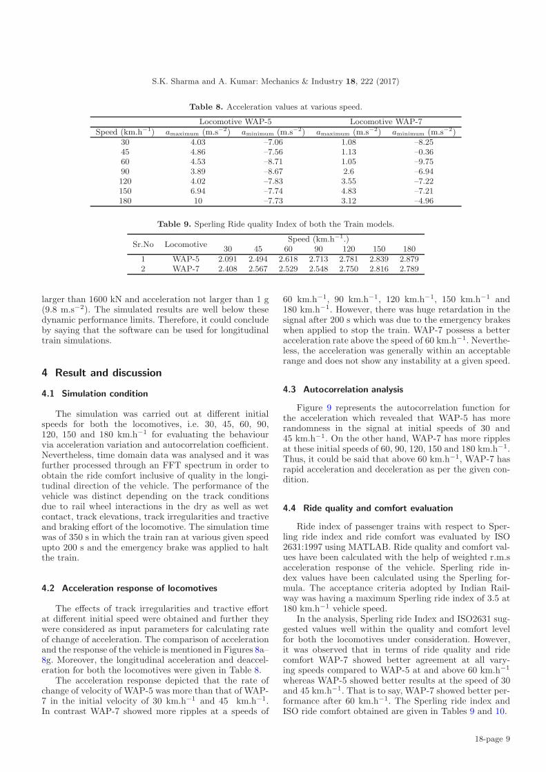
Table 8. Acceleration values at various speed.

Locomotive WAP-5 Locomotive WAP-7

Speed (km.h−1) amaximum (m.s−2) aminimum (m.s−2) amaximum (m.s−2) aminimum (m.s−2)30 4.03 –7.06 1.08 –8.2545 4.86 –7.56 1.13 –0.3660 4.53 –8.71 1.05 –9.7590 3.89 –8.67 2.6 –6.94120 4.02 –7.83 3.55 –7.22150 6.94 –7.74 4.83 –7.21180 10 –7.73 3.12 –4.96

Table 9. Sperling Ride quality Index of both the Train models.

Sr.No LocomotiveSpeed (km.h−1.)

30 45 60 90 120 150 1801 WAP-5 2.091 2.494 2.618 2.713 2.781 2.839 2.8792 WAP-7 2.408 2.567 2.529 2.548 2.750 2.816 2.789

larger than 1600 kN and acceleration not larger than 1 g(9.8 m.s−2). The simulated results are well below thesedynamic performance limits. Therefore, it could concludeby saying that the software can be used for longitudinaltrain simulations.

4 Result and discussion

4.1 Simulation condition

The simulation was carried out at different initialspeeds for both the locomotives, i.e. 30, 45, 60, 90,120, 150 and 180 km.h−1 for evaluating the behaviourvia acceleration variation and autocorrelation coefficient.Nevertheless, time domain data was analysed and it wasfurther processed through an FFT spectrum in order toobtain the ride comfort inclusive of quality in the longi-tudinal direction of the vehicle. The performance of thevehicle was distinct depending on the track conditionsdue to rail wheel interactions in the dry as well as wetcontact, track elevations, track irregularities and tractiveand braking effort of the locomotive. The simulation timewas of 350 s in which the train ran at various given speedupto 200 s and the emergency brake was applied to haltthe train.

4.2 Acceleration response of locomotives

The effects of track irregularities and tractive effortat different initial speed were obtained and further theywere considered as input parameters for calculating rateof change of acceleration. The comparison of accelerationand the response of the vehicle is mentioned in Figures 8a–8g. Moreover, the longitudinal acceleration and deaccel-eration for both the locomotives were given in Table 8.

The acceleration response depicted that the rate ofchange of velocity of WAP-5 was more than that of WAP-7 in the initial velocity of 30 km.h−1 and 45 km.h−1.In contrast WAP-7 showed more ripples at a speeds of

60 km.h−1, 90 km.h−1, 120 km.h−1, 150 km.h−1 and180 km.h−1. However, there was huge retardation in thesignal after 200 s which was due to the emergency brakeswhen applied to stop the train. WAP-7 possess a betteracceleration rate above the speed of 60 km.h−1. Neverthe-less, the acceleration was generally within an acceptablerange and does not show any instability at a given speed.

4.3 Autocorrelation analysis

Figure 9 represents the autocorrelation function forthe acceleration which revealed that WAP-5 has morerandomness in the signal at initial speeds of 30 and45 km.h−1. On the other hand, WAP-7 has more ripplesat these initial speeds of 60, 90, 120, 150 and 180 km.h−1.Thus, it could be said that above 60 km.h−1, WAP-7 hasrapid acceleration and deceleration as per the given con-dition.

4.4 Ride quality and comfort evaluation

Ride index of passenger trains with respect to Sper-ling ride index and ride comfort was evaluated by ISO2631:1997 using MATLAB. Ride quality and comfort val-ues have been calculated with the help of weighted r.m.sacceleration response of the vehicle. Sperling ride in-dex values have been calculated using the Sperling for-mula. The acceptance criteria adopted by Indian Rail-way was having a maximum Sperling ride index of 3.5 at180 km.h−1 vehicle speed.

In the analysis, Sperling ride Index and ISO2631 sug-gested values well within the quality and comfort levelfor both the locomotives under consideration. However,it was observed that in terms of ride quality and ridecomfort WAP-7 showed better agreement at all vary-ing speeds compared to WAP-5 at and above 60 km.h−1

whereas WAP-5 showed better results at the speed of 30and 45 km.h−1. That is to say, WAP-7 showed better per-formance after 60 km.h−1. The Sperling ride index andISO ride comfort obtained are given in Tables 9 and 10.

18-page 9


0 50 100 150 200 250 300 350-10

-8

-6

-4

-2

0

2

4

6

Ac

cel

erat

ion

(m/s

2 )

T ime (s)

8.33 m/s (30 km/h)WAP-5 8.33 m/s (30 km/h)WAP-7

(a)

(a)

0 50 100 150 200 250 300 350-10

-8

-6

-4

-2

0

2

4

6

Ac

cel

erat

ion

(m/s

2 )

T ime (s)

12.5m/s(45km/h)WAP-5 12.5m/s(45km/h)WAP-7

(b)

(b)

0 50 100 150 200 250 300 350-10

-8

-6

-4

-2

0

2

4

6

Ac

cel

erat

ion

(m/s

2 )

T ime (s)


(c)

(c)

0 50 100 150 200 250 300 350-10

-8

-6

-4

-2

0

2

4

6

Ac

cel

erat

ion

(m/s

2 )

T ime (s)

25m/s(90km/h)WAP-5 25m/s(90km/h)WAP-7

(d)

(d)

0 50 100 150 200 250 300 350-10

-8

-6

-4

-2

0

2

4

6

Ac

cel

erat

ion

(m/s

2 )

T ime (s)


(e)

(e)

0 50 100 150 200 250 300 350-10

-8

-6

-4

-2

0

2

4

6

Ac

cel

erat

ion

(m/s

2 )

T ime (s)


(f)

(f)

0 50 100 150 200 250 300 350-10

-8

-6

-4

-2

0

2

4

6

Ac

cel

erat

ion

(m/s

2 )

T ime (s)

50m/s(180km/h)WAP-5 50m/s(180km/h)WAP-7

(g)

(g)

Fig. 8. Vehicle acceleration at speed (a)–(g): 30, 45, 60, 90, 120, 150, 180 km.h−1 respectively.

18-page 10


Table 10. Ride comfort evaluation (ISO 2631) of both the train models.

Speed km.h−1 Locomotive WAP-5 Locomotive WAP-7Ride comfort evaluation

awrms awrms

30 0.083 0.132 comfortable







0 50 100 150 200 250 300 350-0.2

0.0

0.2

0.4

0.6 8.33 m/s (30 km/h)WAP-5 8.33 m/s (30 km/h)WAP-7 12.5m/s(45km/h)WAP-5 12.5m/s(45km/h)WAP-7 16.67m/s(60km/h)WAP-5 16.67m/s(60km/h)WAP-7 25m/s(90km/h)WAP-5 25m/s(90km/h)WAP-7 33.33m/s(120km/h)WAP-5 33.33m/s(120km/h)WAP-7 41.66m/s(150km/h)WAP-5 41.66m/s(150km/h)WAP-7 50m/s(180km/h)WAP-5 50m/s(180km/h)WAP-7

Ac

cel

erat

ion

Aut

o c

orre

lati

on

T ime (s)Fig. 9. Autocorrelation analysis for the acceleration at different initial speed.

5 Conclusion

The analysis of longitudinal train dynamic was doneto evaluate the ride quality and ride comfort. In this pa-per, a comparative analysis was done between WAP-5 andWAP-7 electric locomotives. Rail track corridor betweenMumbai to Ahmedabad (India) was taken into considera-tion. The effect due to TE, BE and variation in the initialspeeds, i.e. 30, 45, 60, 90, 120, 150 and 180 km.h−1 wereanalysed, keeping all the other parameters constant. Inthe suggested analysis, Sperling ride index and ISO2631suggested values were within the quality and comfort levelfor both the locomotives under consideration. However, itcan be observed in the analysis in terms of ride qualityand ride comfort, WAP-7 has shown better agreementat all varying speeds compared to WAP-5 at and above60 km.h−1 whereas WAP-5 performed better at the speedof 30 and 45 km.h−1. It can be concluded from the anal-ysis that WAP-7 performs better above 60 km.h−1.

References

[1] Electric Locomotive Classes – AC WAP7 and WAP-5, 2009, http://www.irfca.org/faq/faq-loco2e.html

(accessed 19 May 2016)[2] S. Pitroda, D. parekh, M. S. Verma, R. Lall, G.

Raghuram, V. Chatterjee, R. Jain, Report of the ExpertGroup for Modernizaion of Indian Railways, Ministry ofRailways, Government of India 2012

[3] Indian locomotive class WAP-5, 2015; https://en.

wikipedia.org/wiki/Indian_locomotive_class_WAP-5

(accessed 03 July 2015)[4] Indian locomotive class WAP-7, 2015 https://en.

wikipedia.org/wiki/Indian_locomotive_class_WAP-7

(accessed 03 July 2016)[5] C. Colin, Longitudinal Train Dynamics, Handbook of

Railway Vehicle Dynamics, CRC Press 2006, pp. 239–277[6] Q. Wu, S. Luo, C. Cole, Longitudinal dynamics and en-

ergy analysis for heavy haul trains, J. Modern Trans. 22(2014) 127–136

18-page 11

http://www.irfca.org/faq/faq-loco2e.html

https://en.wikipedia.org/wiki/Indian_locomotive_class_WAP-5





[7] Y. Sun, C. Cole, M. Spiryagin, T. Godber, S. Hames,M. Rasul, Longitudinal heavy haul train simulationsand energy analysis for typical Australian track routes,Proceedings of the Institution of Mechanical Engineers,Part F: Journal of Rail and Rapid Transit 228 (2013)355–366

[8] L. F. Shampine, Vectorized adaptive quadrature inMATLAB, J. Comput. Appl. Mathem. 211 (2008) 131–140

[9] C. Craciun, T. Mazilu, Simulation of the longitudinal dy-namic forces developed in the body of passenger trains,Ann. Faculty Eng. Hunedoara - Int. J. Eng. 12 (2014)19–26

[10] C. Cruceanu, Train Braking, Reliability and Safetyin Railway, Dr. Xavier Perpinya (Ed.), InTech, 2012.DOI: 10.5772/37552. Available from: http://www.

intechopen.com/books/reliability-and-safety-in-

railway/braking-systems-for-railway-vehicles

[11] M. K. Jain, Train, grade, curve and AccelerationResistance, 2013; https://www.railelectrica.

com/traction-mechanics/train-grade-curve-and-

acceleration-resistance-2/ ( accessed 12 December2015)

[12] K. Chandra, Maintenance manual for BG coaches of LHBdesign, Ministry of Railways, Government of India 2002

[13] A. Swaroop, A technical note in continuation of areasoned document of EOI of AAR ‘H’Type tight-lock

couplers having balanced type draft gear, ResearchDesigns and Standards Organisation, 2011

[14] WAP-5 and WAP-7 tractive effort / braking ef-fort, Technical Data and Notes, Indian Railways,India, 2001. http://www.irfca.org/docs/index.html#

tech (accessed 10-oct, 2015)[15] M. Haag, Autocorrelation of Random Processes, Charlet

Reedstrom, OpenStax Rice University, 2005 https://

cnx.org/contents/cillqc8i@5/Autocorrelation-of-

Random-Proc. (accessed 20 May 2016)[16] T. M. Apostol, Modular functions and Dirichlet series in

number theory, Springer Science & Business Media, 2012[17] R. C. Sharma, Sensitivity Analysis of Ride Behaviour

of Indian Railway Rajdhani Coach using LagrangianDynamics, Int. J. Vehicle Struct. Sys. 5 (2013) 84–89

[18] Y.-T. Fan, W.-F. Wu, Dynamic analysis and ride qualityevaluation of railway vehicles numerical simulation andfield test verification, J. Mech. 22 (2006) 1–11

[19] 12931/mumbai central-Ahmedabad AC double deckerexpress Indian rail info, Indian rail info, 2014.;http://indiarailinfo.com/train/mumbai-central-

ahmedabad-ac-double-decker-express-12931-bct-

to-adi/18711/297/60 ( accessed 10 October 2015)[20] Universal Mechanism software, 2015. http://www.

universalmechanism.com/ (accessed 15 September 2015)[21] Simulation of rail vehicle dynamics user’s manual

Universal Mechanism 7.0 2014

18-page 12

http://www.intechopen.com/books/reliability-and-safety-in-railway/braking-systems-for-railway-vehicles



https://www.railelectrica.com/traction-mechanics/train-grade-curve-and-acceleration-resistance-2/



http://www.irfca.org/docs/index.html#tech

http://www.irfca.org/docs/index.html#tech

https://cnx.org/contents/cillqc8i@5/Autocorrelation-of-Random-Proc.



http://indiarailinfo.com/train/mumbai-central-ahmedabad-ac-double-decker-express-12931-bct-to-adi/18711/297/60



http://www.universalmechanism.com/

http://www.universalmechanism.com/

impact of electric locomotive traction of the passenger

Documents