impact of seismic code provisions in the central u.s.: a

IMPACT OF SEISMIC CODE PROVISIONS IN THE CENTRAL

U.S.: A PERFORMANCE EVALUATION OF A REINFORCED

CONCRETE BUILDING

A Thesis

by

ERIN KUEHT

Submitted to the Office of Graduate Studies of Texas A&M University

in partial fulfillment of the requirements for the degree of

MASTER OF SCIENCE

August 2007

Major Subject: Civil Engineering

IMPACT OF SEISMIC CODE PROVISIONS IN THE CENTRAL

U.S.: A PERFORMANCE EVALUATION OF A REINFORCED

CONCRETE BUILDING

A Thesis

by

ERIN KUEHT

Submitted to the Office of Graduate Studies of Texas A&M University

in partial fulfillment of the requirements for the degree of

MASTER OF SCIENCE

Approved by : Chair of Committee, Mary Beth D. Hueste Committee Members, Joseph M. Bracci Paolo Gardoni Walter Peacock Head of Department, David Rosowsky

August 2007

Major Subject: Civil Engineering

iii

ABSTRACT

Impact of Seismic Code Provisions in the Central U.S.:

A Performance Evaluation of a Reinforced Concrete Building.

(August 2007)

Erin Kueht, B.S. Texas A&M University

Chair of Advisory Committee: Dr. Mary Beth D. Hueste

The close proximity to the New Madrid Seismic Zone and the significant

population and infrastructure presents a potentially substantial risk for central U.S. cities

such as Memphis, Tennessee. However, seismic provisions in currently adopted

Memphis building codes for non-essential structures have a lower seismic design

intensity level than the 2003 International Building Code (IBC) with broader acceptance

nationally. As such, it is important to evaluate structures designed with these local

seismic provisions to determine whether they will perform adequately during two

different design-level earthquakes in this region.

A four-story reinforced concrete (RC) moment frame with wide-module pan

joists was designed according to current building codes relevant to the central U.S.: the

2003 IBC, the City of Memphis and Shelby County locally amended version of the 2003

IBC, and the 1999 Standard Building Code (SBC). Special moment frames (SMFs) were

required for the IBC and SBC designs, but lower design forces in the amended IBC case

study permitted an intermediate moment frame (IMF). However, the margin by which a

SMF was required was very small for the SBC design. For slightly different conditions

IMFs could be used.

Nonlinear push-over and dynamic analyses using synthetic ground motions

developed for Memphis for 2% and 10% probabilities of exceedance in 50 years were

conducted for each of the three designs. The FEMA 356 recommended Basic Safety

Objective (BSO) is to dually achieve Life Safety (LS) for the 10% in 50 years

earthquake and Collapse Prevention (CP) for the 2% in 50 years earthquake. For the

iv

member-level evaluation, the SMF designs met the LS performance objective, but none

of the designs met the CP performance objective or the BSO. However, the margin by

which the SMF buildings exceeded CP performance was relatively small compared to

that of the IMF building. Fragility curves were also developed to provide an estimate of

the probability of exceeding various performance levels and quantitative performance

limits. These relationships further emphasize the benefits of using an SMF as required

by the IBC and, in this case, the SBC.

v

ACKNOWLEDGMENTS

This study was conducted at Texas A&M University and contributes to research

conducted by the Mid-America Earthquake (MAE) Center within the consequence-based

risk management paradigm. This material is based upon work supported under a

National Science Foundation Graduate Research Fellowship. The opinions expressed in

this paper are those of the author and do not necessarily reflect the views or policies of

the sponsors.

I wish to thank my advisor, Dr. Mary Beth Hueste, for her guidance and

encouragement throughout my undergraduate and graduate careers. She has been a first-

rate mentor and I thoroughly appreciate the opportunities she has provided for outreach

and presenting my research on a broader scope. I would also like to gratefully

acknowledge Dr. Joseph Bracci for his help and advice in my research and career goals.

I appreciate the support of my other committee members, Dr. Paolo Gardoni and Dr.

Walter Peacock.

I would like to thank my fellow graduate student, Jong-Wha Bai, for his immense

support in problem solving and gracious answering of my numerous questions, as well

as my other civil engineering graduate student colleagues for their friendship and

support throughout my graduate degree program. Another special thanks goes to my

contacts in the structural engineering consulting industry who answered my technical

questions with extreme patience. Lastly, I thoroughly appreciate the support of all my

family and friends.

vi

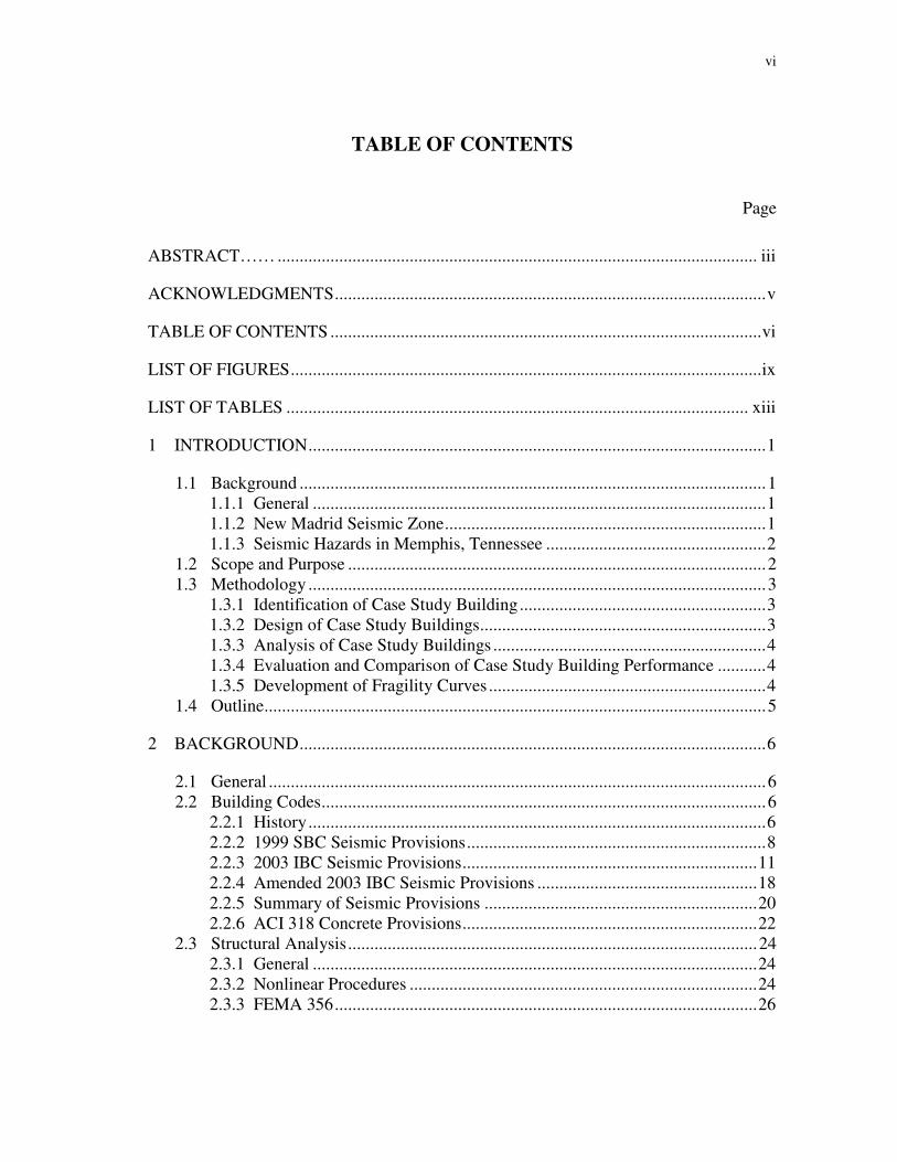
TABLE OF CONTENTS

Page

ABSTRACT…… ............................................................................................................. iii

ACKNOWLEDGMENTS..................................................................................................v

TABLE OF CONTENTS ..................................................................................................vi

LIST OF FIGURES...........................................................................................................ix

LIST OF TABLES ......................................................................................................... xiii

1 INTRODUCTION........................................................................................................1

1.1 Background ..........................................................................................................1 1.1.1 General .......................................................................................................1 1.1.2 New Madrid Seismic Zone.........................................................................1 1.1.3 Seismic Hazards in Memphis, Tennessee ..................................................2

1.2 Scope and Purpose ...............................................................................................2 1.3 Methodology ........................................................................................................3

1.3.1 Identification of Case Study Building........................................................3 1.3.2 Design of Case Study Buildings.................................................................3 1.3.3 Analysis of Case Study Buildings ..............................................................4 1.3.4 Evaluation and Comparison of Case Study Building Performance ...........4 1.3.5 Development of Fragility Curves ...............................................................4

1.4 Outline..................................................................................................................5

2 BACKGROUND..........................................................................................................6

2.1 General .................................................................................................................6 2.2 Building Codes.....................................................................................................6

2.2.1 History........................................................................................................6 2.2.2 1999 SBC Seismic Provisions....................................................................8 2.2.3 2003 IBC Seismic Provisions...................................................................11 2.2.4 Amended 2003 IBC Seismic Provisions ..................................................18 2.2.5 Summary of Seismic Provisions ..............................................................20 2.2.6 ACI 318 Concrete Provisions...................................................................22

2.3 Structural Analysis.............................................................................................24 2.3.1 General .....................................................................................................24 2.3.2 Nonlinear Procedures ...............................................................................24 2.3.3 FEMA 356................................................................................................26

vii

2.3.4 Fragility Curves........................................................................................29 2.4 Vulnerability of Central U.S. Buildings ............................................................32

3 CASE STUDY BUILDING .......................................................................................33

3.1 Introduction........................................................................................................33 3.2 Building Description ..........................................................................................35 3.3 Building Design .................................................................................................36

3.3.1 General .....................................................................................................37 3.3.2 Non-seismic Loads ...................................................................................38 3.3.3 CS1 Seismic Loads...................................................................................42 3.3.4 CS2 Seismic Loads...................................................................................44 3.3.5 CS3 Seismic Loads...................................................................................46 3.3.6 Seismic Load Summary ...........................................................................47

3.4 Analysis for Design Loads.................................................................................48 3.4.1 General .....................................................................................................48 3.4.2 Modeling Assumptions ............................................................................49 3.4.3 Design Fundamental Period .....................................................................50

3.5 Member Design..................................................................................................51 3.5.1 General .....................................................................................................51 3.5.2 Member Dimensions ................................................................................51 3.5.3 Reinforcement ..........................................................................................54 3.5.4 Column-to-Beam Strength Ratios ............................................................64

3.6 Lateral Frame Cost Estimate Comparisons........................................................65

4 NONLINEAR MODELING ......................................................................................68

4.1 Introduction........................................................................................................68 4.2 Analytical Models ..............................................................................................68

4.2.1 General .....................................................................................................68 4.2.2 Building Model ........................................................................................69 4.2.3 Individual Member Modeling ..................................................................72 4.2.4 Confinement Factors ................................................................................74 4.2.5 Loads, Masses and Damping....................................................................77

4.3 Synthetic Ground Motions .................................................................................78

5 ANALYSIS AND EVALUATION ...........................................................................81

5.1 Nonlinear Analysis.............................................................................................81 5.1.1 General .....................................................................................................81 5.1.2 Fundamental Periods ................................................................................81 5.1.3 Push-over Analysis...................................................................................82 5.1.4 Dynamic Analysis ....................................................................................85 5.1.5 Comparison of Push-over and Dynamic Results......................................88

5.2 Performance Evaluation.....................................................................................92

viii

5.2.1 General .....................................................................................................92 5.2.2 Global-level Limits ..................................................................................92 5.2.3 Member-level Limits................................................................................95

6 FRAGILITY ANALYSIS ........................................................................................104

6.1 Introduction......................................................................................................104 6.1.1 Methodology ..........................................................................................104 6.1.2 Additional Ground Motions ...................................................................105

6.2 Qualitative Limits ............................................................................................107 6.2.1 Global-level ............................................................................................107 6.2.2 Member-level .........................................................................................115 6.2.3 Numerical Comparison ..........................................................................128

6.3 Quantitative Limits ..........................................................................................130 6.4 Selection of Default Fragility Curves ..............................................................137

6.4.1 General ...................................................................................................137 6.4.2 Default Fragility Curves.........................................................................137 6.4.3 MAEviz Implementation........................................................................145

7 SUMMARY, CONCLUSIONS AND RECOMMENDATIONS............................148

7.1 Summary ..........................................................................................................148 7.2 Conclusions......................................................................................................149 7.3 Recommendations for Future Research ...........................................................151

REFERENCES…...........................................................................................................153

APPENDIX A GROUND MOTION TIME HISTORIES...........................................158

APPENDIX B MAXIMUM INTERSTORY DRIFTS................................................166

VITA………….. ............................................................................................................174

ix

LIST OF FIGURES

Page

Fig. 2.1. Evolution of seismic design in building codes ...............................................8

Fig. 2.2. Hazard curves for California and Memphis ...................................................19

Fig. 2.3. IBC seismic load cases ...................................................................................21

Fig. 2.4. Fragility curves methodology.........................................................................30

Fig. 2.5. Quantitative drift limit evaluation ..................................................................31

Fig. 3.1. Case study building plan view .......................................................................36

Fig. 3.2. Case study building elevation view...............................................................36

Fig. 3.3. Live load patterns..........................................................................................39

Fig. 3.4. ASCE 7 wind load cases (ASCE 2002) .........................................................40

Fig. 3.5. Typical wind load distribution .......................................................................41

Fig. 3.6. Memphis zip codes.........................................................................................42

Fig. 3.7. Comparison of seismic design coefficients, Cs ..............................................48

Fig. 3.8. ETABS 3-D models .......................................................................................49

Fig. 3.9. Typical wide-module joist cross-section.......................................................54

Fig. 3.10. Typical beam detailing ...................................................................................55

Fig. 3.11. Typical SMF 1st floor N-S exterior beam cross sections...............................61

Fig. 3.12. Typical SMF 1st floor N-S interior beam cross sections ...............................61

Fig. 3.13. Typical IMF 1st floor N-S interior beam cross sections ................................61

Fig. 3.14. Typical IMF 1st floor N-S exterior beam cross sections................................62

Fig. 3.15. Column cross-sections....................................................................................63

Fig. 4.1. Decomposition of a rectangular RC section...................................................69

x

Page

Fig. 4.2. Degrees of freedom and Gauss points of cubic formulation .........................69

Fig. 4.3. ZEUS-NL 2-D frame models .........................................................................70

Fig. 4.4. Typical frame geometry in ZEUS-NL (units in mm).....................................71

Fig. 4.5. Typical node locations for modeling frame members (units in mm).............72

Fig. 4.6. Rigid joint definition ......................................................................................72

Fig. 4.7. ZEUS-NL element cross-sections ..................................................................73

Fig. 4.8. ZEUS-NL material models.............................................................................73

Fig. 4.9. Equivalent point loads applied to E-W members and joists...........................78

Fig. 4.10. Spectral accelerations for Rix-Fernandez ground motions ............................78

Fig. 5.1. Load patterns for push-over analysis .............................................................83

Fig. 5.2. Push-over results (E-W) .................................................................................84

Fig. 5.3. Push-over results (N-S) ..................................................................................85

Fig. 5.4. Comparison of push-over and dynamic analyses (E-W)................................89

Fig. 5.5. Comparison of push-over and dynamic analyses (N-S).................................91

Fig. 5.6. Median maximum interstory drifts (E-W) .....................................................94

Fig. 5.7. Median maximum interstory drifts (N-S).......................................................95

Fig. 5.8. Locations where LS plastic rotation limits are exceeded in CS2 (E-W)........98

Fig. 5.9. Locations where CP plastic rotation limits are exceeded (E-W) ...................99

Fig. 5.10. Locations where LS plastic rotation limits are exceeded in CS2 (N-S).......102

Fig. 5.11. Locations where CP plastic rotation limits are exceeded (N-S)...................103

Fig. 6.1. Spectral accelerations for Wen and Wu ground motions .............................107

Fig. 6.2. Development of global power law equations (E-W)....................................109

Fig. 6.3. Development of global power law equations (N-S).....................................110

xi

Page

Fig. 6.4. Global level fragility curves (E-W)..............................................................113

Fig. 6.5. Global level fragility curves (N-S)...............................................................114

Fig. 6.6. Example loading patterns for member-level push-over analysis .................115

Fig. 6.7. Modal push-over curves and member-level limits (E-W)............................117

Fig. 6.8. Modal push-over curves and member-level limits (N-S).............................118

Fig. 6.9. Critical response push-over curves and member-level limits (E-W) ...........119

Fig. 6.10. Critical response push-over curves and member-level limits (N-S) ............120

Fig. 6.11. Development of member-level power law equations (E-W)........................121

Fig. 6.12. Development of member-level power law equations (N-S).........................122

Fig. 6.13. Modal pattern member-level fragility curves (E-W)....................................124

Fig. 6.14. Modal pattern member-level fragility curves (N-S).....................................125

Fig. 6.15. Critical response member-level fragility curves (E-W) ...............................126

Fig. 6.16. Critical response member-level fragility curves (N-S) ................................127

Fig. 6.17. Triangular push-over curves and quantitative limits (E-W).........................131

Fig. 6.18. Triangular push-over curves and quantitative limits (N-S)..........................132

Fig. 6.19. Locations of inelastic rotation at PMI for triangular push-over (E-W)........133

Fig. 6.20. Locations of inelastic rotation at PMI for triangular push-over (N-S).........134

Fig. 6.21. Quantitative fragility curves (E-W)..............................................................135

Fig. 6.22. Quantitative fragility curves (N-S)...............................................................136

Fig. 6.23. Relationship between performance levels and damage states .....................137

Fig. 6.24. Selection of default fragility curves for CS2 (E-W).....................................139

Fig. 6.25. Default fragility curves for CS1 (E-W)........................................................139


xii

Page




Fig. 6.30. Selection of default fragility curves for CS1 (N-S)......................................142

Fig. 6.31. Default fragility curves for CS1 (N-S) .........................................................142





Fig. 6.36. Comparison of default fragility curves with MAEviz fragility expressions 146

xiii

LIST OF TABLES

Page

Table 2.1. SBC Seismic Performance Categories ..........................................................9

Table 2.2. SBC soil profiles ........................................................................................10

Table 2.3. Coefficient for upper limit on calculated period ........................................11

Table 2.4. Site class definitions ...................................................................................13

Table 2.5. Values of Site Coefficient Fa .....................................................................14

Table 2.6. Values of Site Coefficient Fv ......................................................................14

Table 2.7. Seismic Design Categories based on SDS ...................................................15

Table 2.8. Seismic Design Categories based on SD1 ...................................................15

Table 2.9. Coefficient for upper limit on calculated period ........................................18

Table 2.10. Summarized design procedure ....................................................................20

Table 2.11. Seismic design coefficient, Cs, calculations................................................20

Table 2.12. FEMA 356 acceptance criteria for nonlinear procedures – RC beams controlled by flexure ...................................................................................28

Table 2.13. FEMA 356 acceptance criteria for nonlinear procedures - RC columns controlled by flexure ...................................................................................29

Table 3.1. Post 1990 Shelby County office building inventory ..................................33

Table 3.2. Concrete MRF parameters in Shelby County .............................................34

Table 3.3. Typical Memphis buildings based on engineers’ input...............................34

Table 3.4. Case study buildings and design codes .......................................................37

Table 3.5. Gravity loads ...............................................................................................38

Table 3.6. ASCE 7 Case 1 wind loads .........................................................................40

Table 3.7. Spectral accelerations for various Memphis zip codes ...............................43

xiv

Page

Table 3.8. Calculation of redundancy coefficient for seismic forces in E-W direction.......................................................................................................44

Table 3.9. Comparison of seismic design parameters for CS1 and CS2......................45

Table 3.10. Summary of seismic design parameters ......................................................48

Table 3.11. Controlling E-W design fundamental periods.............................................51

Table 3.12. Typical member sizes..................................................................................52

Table 3.13. Compressive strength of elements...............................................................53

Table 3.14. CS1 N-S interior beam reinforcement.........................................................55

Table 3.15. CS1 N-S exterior beam reinforcement ........................................................56

Table 3.16. CS1 E-W beam reinforcement ....................................................................56







Table 3.23. CS1 negative bar cutoff lengths ..................................................................60



Table 3.26. CS1 column reinforcement..........................................................................63



Table 3.29. Column-to-beam strength ratios..................................................................65

xv

Page

Table 3.30. RS Means material cost data .......................................................................65

Table 3.31. Concrete quantities and costs ......................................................................66

Table 3.32. Reinforcement quantities and costs.............................................................66

Table 4.1. ZEUS-NL material modeling parameter values..........................................74

Table 4.2. ZEUS-NL column confinement factors ......................................................76

Table 4.3. ZEUS-NL beam confinement factors (E-W)...............................................76

Table 4.4. ZEUS-NL beam confinement factors (N-S)................................................77

Table 4.5. 10% in 50 years Rix-Fernandez ground motions ........................................79

Table 4.6. 2% in 50 years Rix-Fernandez ground motions ..........................................80

Table 5.1. Comparison of fundamental periods, T (s) (E-W).......................................82

Table 5.2. ZEUS-NL fundamental periods, T (s) (N-S) ...............................................82

Table 5.3. E-W maximum building drift and base shear ratio (10% in 50 years)........86

Table 5.4. E-W maximum building drift and base shear ratio (2% in 50 years)..........86

Table 5.5. N-S maximum building drift and base shear ratio (10% in 50 years).........87

Table 5.6. N-S maximum building drift and base shear ratio (2% in 50 years)...........88

Table 5.7. Global interstory drift values for concrete frame elements.........................93

Table 5.8. Column plastic rotations (E-W) ..................................................................97

Table 5.9. Exterior frame floor member plastic rotations (E-W).................................97

Table 5.10. Interior frame floor member plastic rotations (E-W) ..................................98

Table 5.11. Column plastic rotations (N-S) .................................................................100

Table 5.12. Exterior frame floor member plastic rotations (N-S) ................................101

Table 5.13. Interior frame floor member plastic rotations (N-S) .................................101

Table 5.14. FEMA 356 BSO evaluation for global and member-level performance...103

xvi

Page

Table 6.1. 10% in 50 years ground motions...............................................................106

Table 6.2. 2% in 50 years ground motions.................................................................106

Table 6.3. Global interstory drift limits......................................................................108

Table 6.4. Reduced 2% in 50 years Wen and Wu motions (CS2 E-W model) ..........111

Table 6.5. Reduced 2% in 50 years Rix-Fernandez motions (CS2 E-W model) .......111

Table 6.6. Qualitative member-level interstory drift limits (E-W) ............................116

Table 6.7. Qualitative member-level interstory drift limits (N-S) .............................116

Table 6.8. Uncertainty parameters for developing the fragility curves......................123

Table 6.9. Probability of exceeding LS for 10% in 50 years Rix-Fernandez motions ......................................................................................................128

Table 6.10. Probability of exceeding LS 10% in 50 years Wen and Wu motions .......128

Table 6.11. Probability of exceeding CP for 2% in 50 years Rix-Fernandez motions 129

Table 6.12. Probability of exceeding CP for 2% in 50 years Wen and Wu motions ...129

Table 6.13. Quantitative interstory drift limits.............................................................131

Table 6.14. Performance levels and corresponding interstory drift (%) limits for default fragility curves ..............................................................................138

Table 6.15. Fragility curve parameters for MAEviz ....................................................147

1

1 INTRODUCTION

1.1 Background

1.1.1 General

Seismic design has progressed significantly over the years due to contributions of

practicing engineers as well as academic and government researchers. Lessons learned

from structural failures in past earthquakes, such as the 1989 Loma Prieta earthquake in

San Francisco and the 1994 Northridge earthquake in the Los Angeles area, combined

with a growing theoretical understanding of earthquakes contributes to the continual

progress of seismic design (Hamburger and Kircher 2000). However, this contemporary

understanding can only improve structural performance in earthquakes if it is applied.

1.1.2 New Madrid Seismic Zone

The New Madrid Seismic Zone (NMSZ) is an intraplate seismic zone located in

the central Mississippi valley extending into four states from northeastern Arkansas to

southern Illinois (CUSEC 2007). It is most well known for three of the five largest

earthquakes to occur in the continental United States in the winter of 1811-1812. From

December 1811 to January 1812, three earthquakes with magnitudes larger than 7.0 on

the Richter scale shook the town of New Madrid, Missouri, with such intensity that

houses were thrown down, large areas sank into the earth, and lakes were permanently

drained. Ground shaking effects were felt over the Eastern U. S., and as far away as

Hartford, Connecticut (Street and Nuttli 1990). Despite the severe ground shaking, there

was little structural damage due to the sparse population and the limited infrastructure in

the region during the early nineteenth century. The population has dramatically

increased since then, and the largest close metropolitan city is Memphis, Tennessee, with

over 911,000 residents in the city and surrounding Shelby County (Census 2000).

_______________

This thesis follows the style and format of the ASCE Journal of Structural Engineering.

2

1.1.3 Seismic Hazards in Memphis, Tennessee

The close proximity to the NMSZ and the relatively large population in this area

presents a potentially substantial risk for Central U.S. cities such as Memphis, Tennessee.

Memphis has been the focus of several loss estimation studies for these reasons, and it

has been shown that another strong New Madrid earthquake would cause substantial

casualties and economic loss. A study conducted by FEMA (1985) estimated multi-

billion dollar direct economic losses for the city of Memphis for an earthquake of

moment magnitude M7.6. In the NCEER Memphis loss assessment report (Abrams and

Shinozuka 1997), over $300 million dollars just in structural repair costs were estimated

for reinforced concrete (RC) and unreinforced masonry (URM) buildings for a M7.5

event. According to the Shelby County building inventory developed by French and

Muthukumar (2004), RC and URM buildings comprise approximately half of the total

non single-family housing building inventory.

Regardless of this prospectively high risk, seismic provisions currently adopted

in the Memphis building codes have a lower design seismic intensity level and building

design category than the 2003 International Building Code (IBC) (ICC 2003), which has

broader acceptance nationally. As such, it is important to evaluate structures designed

according to these local seismic provisions to determine whether they will perform

adequately during a major earthquake in this region. Although many studies have been

conducted to examine the seismic performance of the existing building stock designed

with earlier building codes, there has been little focus on new building construction with

the current buildings codes in the Central U.S. for reinforced concrete joist structures.

1.2 Scope and Purpose

The objectives of this study are to compare the structural vulnerability of a

typical RC frame structure designed according to the three building codes relevant to

new design in the Central U.S.: the 2003 International Building Code, a locally amended

version of the 2003 IBC (City of Memphis and Shelby County 2005), and the 1999

Standard Building Code (SBCCI 1999). Nonlinear push-over and dynamic analyses

were conducted for each of the three designs. Synthetic ground motions for 2% and 10%

3

probabilities of exceedance in 50 years for Memphis, Tennessee, were used in the

dynamic analysis. Fragility curves that link measures of earthquake intensity to the

probability of exceeding specific performance levels were developed using FEMA 356

performance levels as well as quantitative performance criteria to compare the expected

seismic performance of each case study building.

1.3 Methodology

The tasks used to accomplish the objectives are outlined in the following

paragraphs.

1.3.1 Identification of Case Study Building

For a better understanding of current structural design in Memphis, phone

interviews with structural engineers having substantial Memphis design experience were

conducted to determine prevalent structural features and building types. Additionally,

French and Muthukumar (2004) in collaboration with the Mid-America Earthquake

(MAE) Center developed a database for the current building inventory in Shelby County,

Tennessee, with a total of 287,057 building records categorized by building use, square

footage, and year built. Using these sources, a four-story RC moment frame office

building with wide-module joists was chosen as the case study structure.

1.3.2 Design of Case Study Buildings

Three models of the case study structure were designed according to the separate

provisions of the current building codes adopted in Memphis and Shelby County for a

site in downtown Memphis. Case Study 1 (CS1) was designed according to the

provisions of the 2003 International Building Code (IBC), Case Study 2 (CS2) with the

2003 IBC with local amended seismic provisions, and Case Study 3 (CS3) with the

design requirements of the 1999 Standard Building Code (SBC).

Each case study was economically designed in accordance with the

corresponding building code and the American Concrete Institute (ACI) Building Code

Requirements for Reinforced Concrete (ACI 318 1995; 2002). The commercial computer

4

software package ETABS (CSI 2002) was used for the analysis of the structures to

determine member design forces and story deformations. The range of seismic demands

required by each code created variations in structural member layout, member sizes, and

reinforcement quantity and detailing.

1.3.3 Analysis of Case Study Buildings

Nonlinear push-over and dynamic response history analyses were performed

using two-dimensional planar frame models developed with the nonlinear finite element

analysis program, ZEUS-NL (Elnashai 2002). Two types of push-over analyses were

conducted for each case study to capture the range of structural capacity: a rectangular

push-over analysis with equal horizontal forces and a push-over analysis with a vertical

distribution proportional to the fundamental mode shape. The nonlinear dynamic

response history analysis was conducted using sets of synthetic ground motion records

corresponding to 2% and 10% probabilities of exceedance in 50 years for Memphis,

Tennessee. The push-over analysis results were compared to the response history results

to evaluate how well the static analysis represented the dynamic response.

1.3.4 Evaluation and Comparison of Case Study Building Performance

The structural performance criteria provided in FEMA 356 were used for both

global-level and member-level evaluations of the case study building response computed

in the ZEUS-NL analysis. Interstory drifts from the dynamic analysis were compared to

the global drift values suggested by FEMA 356, and plastic rotations at the beam-

column joints from the median ground motion were checked with plastic rotation limits

for the detailed FEMA 356 member-level evaluation. The FEMA 356 Basic Safety

Objective was used to assess acceptable seismic performance for the case studies

designed with the different code provisions.

1.3.5 Development of Fragility Curves

Fragility curves were developed using the approach outlined by Wen et al. (2004)

for the three case studies. The relationship describing demand as a function of seismic

5

intensity was determined from a power law equation fitted to the interstory drift results

of the dynamics analysis versus the corresponding spectral accelerations. To cover a

larger range of seismic demands, the dynamic analysis was expanded to include results

from twenty additional Memphis ground motion records for 2% and 10% probabilities of

exceedance in 50 years, as well as the results from the twenty ground motions used in

the FEMA 356 evaluation. Global-level and member-level performance criteria based on

the FEMA 356 guidelines, as well as quantitative limit states derived using push-over

analyses, were used to define the capacity limits for developing the fragility curves.

1.4 Outline

Section 1 of this thesis includes a brief background, scope, purpose and

methodology. Section 2 summarizes the codes, standards and previous research studies

that contribute and provide background to this investigation. The case study building

description and design parameters are described in Section 3, and the analytical

modeling procedure, assumptions and ground motion data are detailed in Section 4.

Section 5 contains the results from the nonlinear static and dynamic analyses and FEMA

356 evaluation for the three case study buildings. The fragility analysis is discussed in

Section 6. Finally, a summary of results, conclusions and recommendations based on this

research are given in Section 7.

6

2 BACKGROUND

2.1 General

The relevant provisions and background information for the building codes

analyzed in this study are presented in this Section. Literature reviews of research

studies that contribute and correlate with this study are also included to provide

additional background information.

2.2 Building Codes

2.2.1 History

2.2.1.1 General

The first known building code, the Laws of Hammurabi, was written during the

reign of the Mesopotamian ruler Hammurabi in 2285-2242 B.C. Law 229: “If a builder

has built a house for a man and has not made strong his work, and the house he built has

fallen, and he has caused the death of the owner of the house, that builder shall be put to

death.” This was one of the first conditions of performance-based design. Even centuries

later, few changes were made to this building philosophy (Francis and Stone 1998).

During the early twentieth century, the production of explicit model building

codes expanded considerably. Three groups were formed to address structural safety

concerns: the Building Officials and Code Administration (BOCA) in 1915, the

International Conference of Building Officials (ICBO) in 1922, and the Southern

Building Code Congress, International (SBCCI) in 1940. Each of these organizations

established building codes in their particular geographic region. The Uniform Building

Code (UBC) was used west of the Mississippi River, while the National Building Code

(known as BOCA) was utilized in the upper Midwest and northeast. The Standard

Building Code (SBC) was the building code of the South.

7

Each of these building codes reflected the philosophy and character of its

geographic region. Differences in format, content, and appearance created difficulties for

contractors and engineers who worked in more than one region. A call for a single set of

national model codes was initiated by the American Architect’s Association in the 1970s.

The International Code Council (ICC) was formed in 1994 to accomplish this objective.

After much collaboration and deliberation with representatives of the three building

councils, the first International Building Code (IBC) was published in April 2000. With

the development and publication of the IBC, the maintenance and updating of the three

regional building codes was discontinued (Francis and Stone 1998).

2.2.1.2 Seismic Provisions

Due to the frequent number of damaging earthquakes in the Western region, the

UBC was the first model building code to include written seismic regulations in 1927,

although the regulations did not become mandatory until 1961. Elective seismic

provisions did not appear in the SBC until 1976, and mandatory provisions were not

adopted into the main body of the code until 1988 (Beavers 2002).

Natural hazard maps developed by the United States Geological Survey (USGS)

and seismological investigations conducted on behalf of the nuclear power industry

provided clear evidence that earthquakes were not just a problem in California.

Following the 1971 San Fernando earthquake, a national policy for earthquake risk

reduction was created: the National Earthquake Hazard Reduction Program (NEHRP)

(Beavers 2002). In 1994, the SBC and BOCA codes adopted the 1991 NEHRP

Provisions (see Fig. 2.1), in part to a federal executive order preventing federal agencies

from taking space in new buildings that did not conform to the NEHRP Provisions

(Hamburger and Kircher 2000).

In the development process of the IBC from the three regional building codes, it

was decided to use the NEHRP Provisions utilized by BOCA and the SBC as the seismic

provisions. However, the 1991 NEHRP Provisions adopted by the two codes would be

out-of-date by the publication date. In collaboration with the ICC, Building Structural

Safety Council, Structural Engineers Association of California, and American Society of

8

Civil Engineers, the 1997 NEHRP Provisions were developed for adoption into the 2000

IBC. The 2003 IBC seismic provisions were based on the 2000 NEHRP Provisions.

Fig. 2.1. Evolution of seismic design in building codes (adapted from Pezeshk 2004)

2.2.2 1999 SBC Seismic Provisions

2.2.2.1 Design Ground Motions

The seismic provisions in the 1999 Standard Building Code are based on the

1991 NEHRP Provisions (BSSC 1992). Two parameters, the Effective Peak

Acceleration (EPV) and the Effective Peak Velocity (EPV), characterize the intensity of

design ground-shaking, which are related to but not precisely equivalent to peak ground

acceleration and peak ground velocity. The EPA and EPV are proportional to spectral

ordinates for periods in the ranges of 0.1 - 0.5 s and 1 s, respectively.

In the SBC design procedure, the coefficients Aa and Av replace the EPA and

EPV parameters. The value of Aa is determined by dividing the EPA by the gravitational

constant to give a dimensionless coefficient for computing lateral forces. Since EPV is a

velocity with units of in/s the dimensionless coefficient Av is obtained by dividing the

EPV by a velocity-related acceleration coefficient of 0.4/12 in/s. Both quantities

corresponded to a 475-year return period (10% probability of exceedance in 50 years)

San Fernando Earthquake, 1971

ATC, 1978

BSSC, 1985

NEHRP, 1991

NEHRP, 1994

NEHRP, 1997

SBC, 1999

SBC, 1994

IBC, 2000

ANSI, 1982

IBC, 2003

NEHRP, 2000

9

earthquake with 5% damping. It has always been recognized by the BSSC that the maps

and coefficients would be updated with time as design professionals reached a better

understanding about structural performance, risk determination, and seismic hazards

around the country (BSSC 1992).

2.2.2.2 Design Procedure

The Seismic Performance Category (SPC) is based on the building function

(Seismic Hazard Exposure Group) and the peak velocity related acceleration, Av. The

SPC definitions are given in Table 2.1. Soil amplification for the site of a building is not

included in the SPC determination. The SPC dictates seismic detailing requirements, as

well as building height and lateral system limitations.

Table 2.1. SBC Seismic Performance Categories (adapted from SBCCI 1999)

Seismic Hazard Exposure Group Effective Peak Velocity-related Acceleration, Av I II III

Av < 0.05 A A A

0.05 ≤ Av < 0.10 B B C

0.10 ≤ Av < 0.15 C C C

0.15 ≤ Av < 0.20 C D D

0.20 ≤ Av D D E

The most common analysis procedure to calculate seismic design forces in the

SBC is the equivalent lateral force procedure. According to SBC Section 1607.4, the

seismic base shear, V, is calculated using Eq. (2.1) with an upper limit of Eq. (2.2). Soil

effects are not included in the upper limit base shear equation, which controls for

buildings with very short periods. The SBC does not magnify the base shear for essential

or hazardous buildings with an importance factor as in the IBC. A percentage of the base

shear is distributed to each story based on the story mass and height.

10

2 / 3

1.2 v

A SV W

RT= (2.1)

0.5 a

AV W

R≤ (2.2)

where:

Av = Coefficient representing effective peak velocity-related acceleration

Aa = Coefficient representing effective peak acceleration S = Coefficient for the soil profile characteristics of the site R = Response modification factor T = Fundamental period of vibration of the structure in seconds in

the direction under consideration W = Seismic weight of the structure

There are four classifications of soil types in the SBC: rock, intermediate soil,

soft soil, and very soft soil. These soil profile types correspond to site coefficients

ranging from 1.0 to 2.0 (see Table 2.2) to amplify the base shear based on soil effects at

the site. According to Dr. Glenn Rix of the Georgia Institute of Technology, a researcher

for the Mid-America Earthquake Center, the soil deposits in Memphis are about 3,000 ft.

deep and are generally stable deposits of sands, gravels, or stiff clays (personal

communication, Feb. 24, 2006).

Table 2.2. SBC soil profiles (adapted from SBCCI 1999)

Soil type Description S

S1

Rock of any characteristic, either shale-like or crystalline in nature, which has a shear wave velocity greater than 2,500 ft/s or stiff soil conditions where the soil depth is less than 200 ft. and the soil types overlaying rock are stable deposits of sands, gravel or stiff clays

1.0

S2

Deep cohesionlesss or stiff clay conditions, where the soil depth exceeds 200 ft. and soil types overlaying rock are stable deposits of sands, gravels, or stiff clays.

1.2

S3 20 to 40 ft. in thickness of soft to medium-stiff clays with or without intervening layers of cohesionless soils

1.5

S4 Shear wave velocity of less than 500 ft/s containing more than 40 ft. of soft clay.

2.0

11

2.2.2.3 Fundamental Period

The upper limit for the period calculated using SBC Section 1607.4.1.2.1 is

shown in Eq. (2.3) for a concrete moment-resisting frame. The code specifies an upper

limit for the structural period (see Table 2.3) used in calculating the base shear to ensure

a conservative design. The upper limit coefficient is based on the mapped effective peak

velocity related coefficient, Av.

Tmax = Ca0.03(hn)

3/4 (2.3)

where:

Ca = Upper limit coefficient hn = Height from the base (ft.)

Table 2.3. Coefficient for upper limit on calculated period (adapted from SBCCI 1999)

Av Upper limit coefficient, Ca

0.4 1.2

0.3 1.3

0.2 1.4

0.15 1.5

0.1 1.7

0.05 1.7

2.2.3 2003 IBC Seismic Provisions

2.2.3.1 Design Ground Motion

In coordination with the development of the 2000 IBC, the 1997 NEHRP

Provisions underwent significant changes including the development of new site factors,

new USGS hazard mapping, and individual advances in design provisions for the major

structural systems and materials (Holmes 2000). One of the most significant changes to

the 1997 provisions is the updated seismic maps (BSSC 1998). Significant earthquake

12

data was discovered in the 20 or more years since the coefficient design maps in the

earlier editions of the NEHRP Provisions were developed. These advances were

incorporated into the new design procedure involving maps based on short-period and

long-period response spectral accelerations.

The 1997 maps define the maximum considered earthquake (MCE) ground

motion for use in design procedures to provide an approximate uniform margin against

collapse (BSSC 1998). The MCE ground motions are based on a set of rules that depend

on the seismicity of an individual region with a focus on ground motions rather than

earthquake magnitude. The MCE ground motions are uniformly defined as the

maximum level of earthquake ground shaking that is considered reasonable to design

structures to resist. For most of the country, the MCE is based on a 2% probability of

exceedance in 50 years ground motion. This design approach provides an approximate

uniform margin against collapse throughout the U.S. (Leyendecker et al. 2000).

The goal of the new seismic maps was to provide for life safety during the design

earthquake and collapse prevention for the MCE ground motion. To determine the

difference between these two performance levels, an intensive study of actual building

performance in earthquakes was conducted. A “seismic margin” was determined by the

Seismic Design Provisions Group based on past structural performance in California

earthquakes, which were designed for the 10% in 50 years earthquake. Structures were

determined to have a low likelihood of collapse for a ground motion 1.5 times the design

earthquake. Therefore, a factor of 2/3 (1/1.5) was multiplied by the MCE to design for

life safety, but ensure collapse prevention at the MCE (Leyendecker et al. 2000).

13

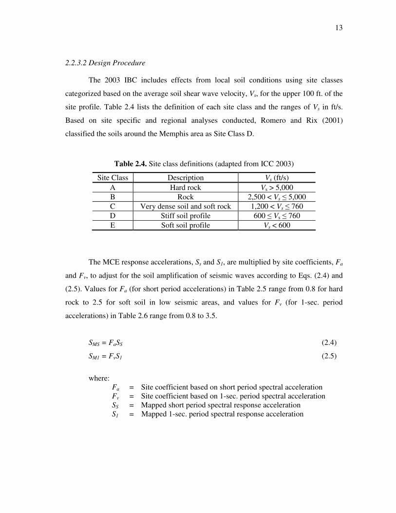
2.2.3.2 Design Procedure

The 2003 IBC includes effects from local soil conditions using site classes

categorized based on the average soil shear wave velocity, Vs, for the upper 100 ft. of the

site profile. Table 2.4 lists the definition of each site class and the ranges of Vs in ft/s.

Based on site specific and regional analyses conducted, Romero and Rix (2001)

classified the soils around the Memphis area as Site Class D.

Table 2.4. Site class definitions (adapted from ICC 2003)

Site Class Description Vs (ft/s)

A Hard rock Vs > 5,000

B Rock 2,500 < Vs ≤ 5,000

C Very dense soil and soft rock 1,200 < Vs ≤ 760

D Stiff soil profile 600 ≤ Vs ≤ 760

E Soft soil profile Vs < 600

The MCE response accelerations, Ss and S1, are multiplied by site coefficients, Fa

and Fv, to adjust for the soil amplification of seismic waves according to Eqs. (2.4) and

(2.5). Values for Fa (for short period accelerations) in Table 2.5 range from 0.8 for hard

rock to 2.5 for soft soil in low seismic areas, and values for Fv (for 1-sec. period

accelerations) in Table 2.6 range from 0.8 to 3.5.

SMS = FaSS (2.4)

SM1 = FvS1 (2.5)

where:

Fa = Site coefficient based on short period spectral acceleration Fv = Site coefficient based on 1-sec. period spectral acceleration SS = Mapped short period spectral response acceleration S1 = Mapped 1-sec. period spectral response acceleration

14

Table 2.5. Values of Site Coefficient Fa (adapted from ICC 2003)

Mapped spectral accelerations at short periods Site Class SS ≤ 0.25 SS = 0.5 SS = 0.75 SS = 1.00 SS ≥ 1.25

A 0.8 0.8 0.8 0.8 0.8

B 1.0 1.0 1.0 1.0 1.0

C 1.2 1.2 1.1 1.0 1.0

D 1.6 1.4 1.2 1.1 1.0

E 2.5 1.7 1.2 0.9 0.9

F Site specific analysis needed

Note: Use straight-line interpolation for intermediate values.

Table 2.6. Values of Site Coefficient Fv (adapted from ICC 2003)

Mapped spectral accelerations at 1-sec. periods Site Class S1 ≤ 0.1 S1 = 0.2 S1 = 0.3 S1 = 0.4 S1 ≥ 0.5

A 0.8 0.8 0.8 0.8 0.8

B 1.0 1.0 1.0 1.0 1.0

C 1.7 1.6 1.5 1.4 1.3

D 2.4 2.0 1.8 1.6 1.5

E 3.5 3.2 2.8 2.4 2.4

F Site specific analysis needed

Note: Use straight-line interpolation for intermediate values.

The adjusted spectral accelerations are multiplied by the reciprocal of the seismic

margin in Eqs. (2.6) and (2.7) to obtain the design spectral response accelerations, which

are used to calculate V and the Seismic Design Category (SDC).

SDS = ⅔SMS (2.6)

SD1 = ⅔SM1 (2.7)

where:

SMS = Adjusted MCE short period spectral response accelerations SM1 = Adjusted MCE 1-sec. period spectral response accelerations

15

Seismic Design Categories determine detailing requirements, structural system

restrictions, height limitations, and analysis procedures for irregular structures. The SDC

is assigned based on the Seismic Use Group, which depends on the function of the

building and how much damage is acceptable after an earthquake, as well as the amount

of ground shaking expected at the site. Unlike the Seismic Performance Category in the

SBC, the SDC includes the effect of soil amplification on the building performance

during a seismic event. The maximum SDC value from Table 2.7 and Table 2.8 controls.

Table 2.7. Seismic Design Categories based on SDS (adapted from ICC 2003)

Seismic Use Group Value of SDS

I II III

SDS < 0.167g A A A

0.167g ≤ SDS < 0.33g B B C

0.33g ≤ SDS < 0.50g C C D

0.50g ≤ SDS D D D

Table 2.8. Seismic Design Categories based on SD1 (adapted from ICC 2003)

Seismic Use Group Value of SD1

I II III

SD1 < 0.067g A A A

0.067g ≤ SD1 < 0.133g B B C

0.133g ≤ SD1 < 0.20g C C D

0.20g ≤ SD1 D D D

The equivalent lateral force procedure can be used for analysis of all structures

except irregular structures in SDC D or higher. The 2003 IBC references ASCE

Minimum Design Loads for Buildings and Other Structures (ASCE 7-02) (ASCE 2002)

for seismic load analysis procedures. The seismic base shear, V, is determined using Eqs.

(2.8) and (2.9) with the limitation of Eq. (2.10). A lower limit of 0.44SDSIW is also

imposed on V. The response modification factor, R, depends on the building type and is

16

intended to reduce the base shear for buildings with greater seismic detailing and

ductility. An occupancy importance factor, IE, is included in the base shear equations to

provide for higher seismic performance for critical facilities.

V = CsW (2.8)

DS

s

E

SC

RI

=

(2.9)

1 D

s

E

SC

RTI

≤

(2.10)

where:

W = Effective seismic weight of the structure Cs = Seismic response coefficient SDS = Design short period spectral response acceleration IE = Occupancy importance factor R = Response modification factor SD1 = Design 1-sec. period spectral response acceleration T = Fundamental period of vibration of the building in the direction

under consideration (s)

The combined effect of horizontal and vertical earthquake-induced forces, E, in

the load combinations represents the ground acceleration in both directions shown in Eq.

(2.11). The effect of horizontal seismic forces, QE, are the forces applied to each story as

a percentage of the total base shear. In high seismic areas, these lateral loads are further

amplified for structures without multiple lateral elements or without an equitable

distribution of lateral elements throughout the structure by the redundancy coefficient, ρ.

0.2E DSE Q S Dρ= ± (2.11)

where:

D = Dead load ρ = Redundancy coefficient QE = Effect of horizontal seismic forces SDS = Design short period spectral response acceleration

17

The redundancy coefficient is determined by the ratio of the design shear resisted

by the most heavily loaded single element to the total shear for a story and the tributary

area of that element. For moment frames, this ratio is represented by the maximum of the

sum of the shears in any two adjacent columns in the plane of a moment frame for a

given direction of loading. The value of ρ is 1.0 for SDC A to C. For SDC D and higher,

ρ is calculated using Eq. (2.12). The redundancy coefficient also affects the number of

lateral resisting members in a particular direction. For concrete moment frame structures,

if ρ is calculated to be greater than 1.25, additional moment frames are needed to

distribute the lateral forces more evenly to reduce ρ to below 1.25.

max

202

x

x

xr A

ρ = − (2.12)

where:

r max x = Maximum sum of the shears in any two adjacent columns in the

plane of a moment frame divided by the total story shear Ax = Floor area of the diaphragm level immediately above the story

2.2.3.3 Fundamental Period

The upper limit for the fundamental period for an RC moment frames is

calculated using Eq. (2.13) where the upper limit coefficient, Cu, depends on the 1-sec.

spectral design acceleration (see Table 2.9), which is different for the 2003 IBC with and

without the local amendments.

Tmax = Cu(0.016)(hn)0.9 (2.13)

where:

Cu = Upper limit coefficient hn = Height from the base (ft.)

18

Table 2.9. Coefficient for upper limit on calculated period (adapted from ICC 2003)

SD1 Upper limit coefficient, Cu

≥ 0.3 1.4

0.2 1.5

0.15 1.6

0.1 1.7

≤ 0.05 1.7

2.2.4 Amended 2003 IBC Seismic Provisions

For California and the rest of the west coast, the 2% in 50 years ground motion

(the MCE used in the 2003 IBC) is approximately 1.5 times the 10% in 50 years ground

motion. When the MCE is multiplied by seismic margin of 2/3 (1/1.5), the design

earthquake becomes approximately a 10% in 50 years hazard for the western U.S. In the

Central U.S., however, the 2% in 50 years earthquake is approximately 4 to 5 times

larger than the 10% in 50 years earthquake (Dowty and Ghosh 2002). This comparison is

shown in Fig. 2.2 for the short period spectral accelerations for the cities of Los Angeles,

San Francisco, and Memphis. Therefore, the use of 2/3 of the MCE design earthquake in

the IBC provisions led to a significantly greater demand for Memphis and the Central

U.S. relative to the previous code provisions. This subject has been hotly debated in this

region, and in the local seismic amendments, Memphis replaced the 2/3 MCE design

earthquake with the 10% in 50 years ground motion.

19

2%

in

50

yea

rs

10

% i

n 5

0 y

ears

.

0.01

0.1

1

10

0.000010.00010.0010.010.1

Annual Frequency of Exceedance

0.2

s S

pec

tral

Acc

eler

atio

n, %

g .

Los Angeles San Fransisco Memphis

California

~ 1.5Memphis

~ 4.8

Fig. 2.2. Hazard curves for California and Memphis (adapted from Leyendecker et al. 2000)

Applying the Memphis amended seismic provisions, Eqs. (2.4) and (2.5) become

Eqs. (2.14) and (2.15). The prime symbol ( ' ) denotes parameters that changed for the

amended IBC. The spectral accelerations for Memphis are reduced by almost 75 percent

from 0.28g to 0.07g for 1-sec. period accelerations and 0.93g to 0.29g for short period

accelerations under the amendments.

SDS' = SMS ' (2.14)

SD1' = SM1 ' (2.15)

where: SMS' = Maximum considered earthquake short period spectral response

accelerations SM1' = Maximum considered earthquake 1-sec. period spectral response

accelerations

The change in the mapped spectral accelerations for the local amendments also

impacts the Seismic Design Category and has a major influence on the structural

members and performance of a structure.

20

2.2.5 Summary of Seismic Provisions

The seismic design procedures outlined in each code are listed in Table 2.10. The

seismic design coefficient, Cs, calculations for the 2003 IBC and 1999 SBC are shown in

Table 2.11. The SBC calculations do not include the Importance Factor, IE, which

increases design forces for essential facilities such as hospitals and hazardous buildings

to provide for better performance. There are no lower limits on the base shear for the

SBC design. Amplification for soil conditions is also more detailed for the IBC design

procedure.

Table 2.10. Summarized design procedure

Parameter 2003 IBC Amended 2003 IBC 1999 SBC

Design map values S1, SS S1 ', SS ' Aa, Av

Design hazard level ⅔ [2% in 50 years] 10% in 50 years 10% in 50 years

Adjusted for soils Fa, Fv Fa ', Fv '

S

Base shear V = CSW

Table 2.11. Seismic design coefficient, Cs, calculations

Building Code Parameter

2003 IBC 1999 SBC

Cs /

DS

E

S

R I

23

1.2 vA S

RT

Upper limit Cs ( )

1

/

D

E

S

T R I

2.5 aA

R

Lower limit Cs

0.044SDSIE None

Lower limit, High seismic

10.5

/ E

S

R I None

21

Once the total base shear is determined for each code, it is distributed to each

level through the lateral force, Fx, calculated as a percentage of the base shear using Eqs.

(2.16) and (2.17).

X VXF C V= (2.16)

1

k

x x

VX nk

i i

i

w hC

w h=

=

∑ (2.17)

where: CVX = Vertical distribution factor V = Design seismic base shear

wx, wi = Portion of the total gravity load of the building, W, located or assigned to level i or x

hx,hi = Height from the base to level i or x (ft.) k = Exponent related to the period of the building

The seismic lateral forces are applied both directly at the center of mass on the

building and at a 5 percent eccentricity of the building length, L, or width, W, from the

center of mass to account for accidental torsion. This results in the total of six seismic

load cases shown in Fig. 2.3.

Fig. 2.3. IBC seismic load cases

22

An allowable drift limit of 2% is imposed in all three seismic code provisions on

the design story drift, ∆, which is defined as the difference of the deflections of the

center of the mass on the top and bottom of the story under consideration. The drift at

level x, δx, is determined from Eq. (2.18).

d xe

x

E

C

I

δδ = (2.18)

where:

δxe = Diaphragm deflection from elastic analysis IE = Occupancy importance factor Cd = Deflection amplification factor in 2003 IBC Table 1617.6

2.2.6 ACI 318 Concrete Provisions

Two different ACI 318 provisions were used in this study; the 2003 IBC

references ACI 318-02 (ACI Committee 318 2002) as the concrete standard, while the

1999 SBC references ACI 318-95 (ACI Committee 318 1995). Most of the applicable

design procedures are the same, except for load factors and moment redistribution

procedures.

ACI 318 Chapter 21 specifies the special seismic detailing provisions for special

moment frames (SMFs) and intermediate moment frames (IMFs). Sections 21.2 through

21.10 provide SMF detailing requirements to improve seismic performance and prevent

the occurrence of story mechanisms in strong earthquakes. The IMF detailing

requirements given in Section 21.12 are less stringent than the SMF requirements, but

still provide for some ductility in an earthquake.

2.2.6.1 SMF Detailing Requirements

Special moment frames are required by the IBC and SBC for SDC D concrete

frame structures and have the most detailed requirements for seismic performance.

According to ACI 318 Section 21.3.2.2, flexural members of a SMF shall have a positive

moment strength at the joint face that is not less than one-half the negative moment

23

strength. The minimum moment strength at any section shall not be less than one-fourth

of the maximum moment strength. Two bars must be provided continuously both top

and bottom for structural integrity.

Seismic hoops must be provided within twice the member depth from the column

face, which is the approximate length of the plastic hinge zone (PHZ), and the first hoop

must be placed within 2 in. of the column face. The spacing of the seismic hoops within

the PHZ must be less than d/4, where d is the distance between the tension reinforcement

and the compression face of the concrete. In this region, every other longitudinal bar

must be supported by a cross-tie with a maximum spacing of 6 in. between transverse

reinforcement. Outside the PHZ, the spacing of the seismic stirrups is determined by the

shear demand with a maximum spacing of d/2. Two-legged stirrups are allowed in this

region.

The SMF joint requirements are provided in ACI 318 Section 21.5. The column

width must be greater than 20 times the diameter of the largest longitudinal bar. The

shear demand of the joint is calculated based on the assumption that the stress in the

flexural tensile reinforcement is 1.25fy. The shear strength depends only on the effective

joint area, concrete compressive strength, and amount of joint confinement per ACI 318

Section 21.5.3. A joint is considered confined if the beam widths framing into it are at

least three-fourths of the column width.

ACI stipulates a strong-column weak-beam design strategy to prevent story

mechanisms from forming. In the vertical plane of the frame considered, the sum of the

nominal flexural strength of the columns at the face of the joint is required to be at least

1.2 times the sum of the beam nominal flexural strength described in Eq. (2.19).

65nc nbM M≥∑ ∑ (2.19)

where:

Mnb = Nominal flexural strength of beam including the slab in tension framing into a joint in a plane

Mnc = Nominal flexural strength of column framing into the joint for the factored axial load consistent with the lateral force direction

24

2.2.6.2 IMF Detailing Requirements

The IMF detailing requirements in ACI 318 Section 21.12 are less stringent than

those for SMFs. The positive moment strength of beams at the face of the joint must be

greater than one-third of the negative moment strength at the joint, and the minimum

moment strength at any section shall not be less than one-fifth the maximum moment

strength.

Joint confinement requirements do not apply to an IMF, which allows smaller

columns and possily a lower concrete strength. The PHZ transverse beam reinforcement

requirements are the same as the SMF, except that every other longitudinal bar does not

have to be laterally supported. IMF column requirements allow larger transverse

reinforcement spacing than SMF columns.

2.3 Structural Analysis

2.3.1 General

Out of the four seismic analysis procedures specified in NEHRP Recommended

Provisions for Seismic Regulations of New Buildings And Other Structures, Part 1:

Provisions (FEMA 450) (BSSC 2004), only the linear response history procedure and

the nonlinear response history procedure predict the response of a structure subjected to

ground motion records. Linear analysis procedures, however, are not capable of

representing the inelastic responses predicted for buildings under large demands from

earthquake loading. Therefore, nonlinear analysis procedures are used in this study to

more accurately predict the seismic performance of the case study buildings.

2.3.2 Nonlinear Procedures

A nonlinear static procedure, commonly called a push-over analysis, involves

monotonically applying lateral load to a structure until a specified displacement is

reached or an instability occurs due to large inelastic deformations. The push-over

analysis can be used to obtain the overall capacity of the structure including yield

25

displacement, peak base shear, as well investigating story mechanisms and the location

of critical members (Jeong and Elnashai 2005).

In the nonlinear dynamic (response history) analysis, ground accelerations are

applied at base of the structure in a finite element analysis to predict the structural

response for the earthquake motions. The response history analysis is considered to be

more accurate than a static analysis because it accounts for the dynamic response of the

structure. However, the response can be highly sensitive to the characteristics of a

particular ground motion. For a better estimate of the dynamic response for a particular

magnitude event or recurrence interval, the median response of multiple ground motions

should be used. FEMA 450 requires at least three ground motions for a response history

analysis, and at least seven ground motion records are needed to use the median response

instead of the maximum response.

Mwafy and Elnashai (2001) investigated the uniform, modal, and inverted

triangular lateral load patterns in a push-over analysis compared with an incremental

inelastic dynamic analysis for twelve RC buildings with different configurations. The

findings indicated that push-over analyses provide insight on the inelastic response of

buildings subjected to ground motions, especially for low rise RC buildings. The benefit

of using more than one load pattern to capture a broader range of expected response was

emphasized.

The basic concepts of the push-over analysis including lateral load patterns and

practical applications were summarized by Krawinkler and Seneviratna (1998). Push-

over drifts were compared with results from a response history analysis with nine ground

motions for a four story steel moment frame building. It was concluded that push-over

analyses can be helpful in exposing design weakness such as story mechanisms,

especially in buildings that vibrate primarily in the first mode. However, additional

evaluation procedures such as inelastic dynamic analysis should be conducted in

conjunction with a push-over analysis for increased accuracy in predicting the dynamic

response.

26

Kalkan and Kunnath (2006) evaluated four types of nonlinear static procedures

using existing 6 and 13 story steel moment frames and 7 and 20 story RC moment frame

buildings. A response history analysis with thirty ground motions was also used for

comparison in the evaluation. The results showed that push-over analyses are more

accurate in lower stories of taller buildings, but when higher modes contributions

become significant, peak roof displacement and interstory drifts can be misrepresented.

Sadjadi et al. (2007) also used nonlinear response history and push-over analyses

to investigate the seismic vulnerability of ductile, nominally-ductile, and gravity load

designed RC moment frame buildings designed with Canadian building codes. Many

other studies which are too numerous to mention have established the common practice

of using both nonlinear static and response history analysis procedures to investigate the

seismic vulnerability of buildings.

2.3.3 FEMA 356

2.3.3.1 General

The Prestandard and Commentary for the Seismic Rehabilitation of Buildings –

FEMA 356 (ASCE 2000) proposed limits for the seismic evaluation of building

structures. FEMA 356 uses target performance levels at certain recurrence intervals to

define the Basic Safety Objective (BSO). Typical global interstory drift values are

suggested as guidance for various building types and plastic rotation limits are provided

for more detailed member-level evaluations.

2.3.3.2 Basic Safety Objective

Three target building performance levels are set based on the amount of damage

a structure sustains during an earthquake:

(1) Immediate Occupancy (IO) – Very limited structural damage has occurred and the structure is safe and functional immediately following the earthquake

(2) Life Safety (LS) – Structural damage occurs, but a significant margin of safety against collapse still remains

27

(3) Collapse Prevention (CP) – Building will continue to support gravity loads, but without a margin against collapse

FEMA 356 defines the BSO as dually meeting the LS performance level under a

10% probability of exceedance in 50 years event and the CP performance level under a

2% probability of exceedance in 50 years event. This objective is intended to allow

limited damage for frequent but moderate earthquakes, with significantly more damage

for higher intensity, infrequent earthquakes.

2.3.3.3 Global and Member-Level Criteria

Intertory drift values are provided for the three structural performance levels to

give an estimation of the global seismic performance for various concrete, steel and

masonry building types. The interstory drifts associated with IO, LS and CP

performance are 1%, 2% and 4%, respectively, for concrete frames. These drift values

are suggested for structures that are designed and detailed for higher seismic demands,

such as SMFs. For structures that are not specially detailed for seismic loading, smaller

global drift values are more appropriate to meet the respective performance levels.

Ramamoorthy et al. (2006) proposed using reduced interstory drift values of 0.5%, 1%

and 2% for the IO, LS and CP performance levels, respectively, for gravity designed

buildings with insufficient column-to-beam strength ratios and section detailing. These

lower values are based on the FEMA 356 member plastic rotation limits, which are

smaller for buildings without special detailing.

The primary evaluation measures in FEMA 356 are member-level acceptance

criteria for concrete, steel, masonry, and wood and light metal framing construction for

various types of elements. These limits are considered more accurate than the global

drift values because they are refined to reflect member design details. Chapter 6

specifies plastic rotation limits for beams, columns, and beam-column joints for RC

moment frames. Plastic rotation is defined as the inelastic rotation beyond the yield

rotation of the member. Tables 2.12 and 2.13 provide the FEMA 356 plastic rotation

28

acceptance criteria to use with nonlinear procedures when evaluating RC beams and

columns controlled by flexure.

Table 2.12. FEMA 356 acceptance criteria for nonlinear procedures – RC beams controlled by flexure (adapted from ASCE 2000)

Plastic rotation acceptance criteria (rad.) 2

Performance level

Component type

Primary Secondary

Conditions

IO LS CP LS CP

'

bal

ρ ρ

ρ

− Transverse Reinforce-

ment1 'w c

V

b d f

≤ 0.0 C ≤ 3 0.01 0.02 0.025 0.02 0.05

≤ 0.0 C ≥ 6 0.005 0.01 0.02 0.02 0.04

≥ 0.5 C ≤ 3 0.005 0.01 0.02 0.02 0.03

≥ 0.5 C ≥ 6 0.005 0.005 0.015 0.015 0.02

≤ 0.0 NC ≤ 3 0.005 0.01 0.02 0.02 0.03

≤ 0.0 NC ≥ 6 0.0015 0.005 0.01 0.01 0.015

≥ 0.5 NC ≤ 3 0.005 0.01 0.01 0.01 0.015

≥ 0.5 NC ≥ 6 0.0015 0.005 0.005 0.005 0.01 Notes: 1. "C" and "NC" are abbreviations for conforming and nonconforming transverse

reinforcement. A component is conforming if, within the flexural plastic hinge region, hoops are spaced at ≤ d/3, and if, for components of moderate and high ductility demand, the strength provided by the hoops (Vs) is at least three-fourths of the design shear. Otherwise, the component is considered nonconforming.

2. Linear interpolation between values listed in the table shall be permitted.

29

Table 2.13. FEMA 356 acceptance criteria for nonlinear procedures - RC columns controlled by flexure (adapted from ASCE 2000)

Plastic rotation acceptance criteria (rad.) 2

Performance level

Component type

Primary Secondary

Conditions

IO LS CP LS CP

'g c

P

A f Transverse reinforce-

ment1 'w c

V

b d f

≤ 0.1 C ≤ 3 0.005 0.015 0.02 0.02 0.03

≤ 0.1 C ≥ 6 0.005 0.012 0.016 0.016 0.024

≥ 0.4 C ≤ 3 0.003 0.012 0.015 0.018 0.025

≥ 0.4 C ≥ 6 0.003 0.01 0.012 0.013 0.02

≤ 0.1 NC ≤ 3 0.005 0.005 0.006 0.01 0.015

≤ 0.1 NC ≥ 6 0.005 0.004 0.005 0.008 0.012

≥ 0.4 NC ≤ 3 0.002 0.002 0.003 0.006 0.01

≥ 0.4 NC ≥ 6 0.002 0.002 0.002 0.005 0.008 Notes: 1. "C" and "NC" are abbreviations for conforming and nonconforming transverse

reinforcement. A component is conforming if, within the flexural plastic hinge region, hoops are spaced at ≤ d/3, and if, for components of moderate and high ductility demand, the strength provided by the hoops (Vs) is at least three-fourths of the design shear. Otherwise, the component is considered nonconforming.

2. Linear interpolation between values listed in the table shall be permitted.

2.3.4 Fragility Curves

The fragility of a component or system is defined as “the conditional probability

of attaining a performance limit state given the occurrence of a particular environmental

demand,” (Wen et al. 2003). Limit states represent a state of unsatisfactory performance,

defined in terms of engineering parameters such as forces or deformations. The

environmental demand in this study is expressed in terms of seismic intensity. The

process for developing fragility curves is shown in Fig. 2.4. To capture a broad scope of

earthquake demand, ground motions with a range of intensities reflecting the seismicity

of the region are needed.

30

Selection of Building Configuration, Material Properties

Design and Analytical Idealization of the Structure

Ground Motion

Uncertainty

Dynamic Analysis

Damage Quantification

Fragility Curves

Push-over

Analysis

Limit State

Definition

Structural

Variability

Selection of Building Configuration, Material Properties

Design and Analytical Idealization of the Structure

Ground Motion

Uncertainty

Dynamic Analysis

Damage Quantification

Fragility Curves

Push-over

Analysis

Limit State

Definition

Structural

Variability

Fig. 2.4. Fragility curves methodology (adapted from Erberik and Elnashai 2004)

The probability of reaching a specified limit state (LS) is calculated using the

following equation (Wen et al. 2004):

P[LS] = Σ P[LS|D=d] P[D=d] (2.20)

where:

LS = Limit state D = Spectrum of uncertain hazards d = Control of interface variable, such as occurrence of a

specific hazard intensity P[LS|D=d] = Fragility P[D=d] = Seismic Hazard

Cornell et al. (2002) and Wen et al. (2004) used the power model in Eq. (2.21) to

predict the seismic demand, D, in the fragility definition. Regression analysis of the

response history results along with corresponding earthquake intensities is conducted to

obtain the power equation parameters.

1

0 ( )a

D S eαα= (2.21)

where: Sa = Spectral acceleration

31

0 1,α α = Parameters determined by regression analysis

e = Unit median error term that describes uncertainty in the relationship

According to Wen et al. (2004), limit states based on interstory drifts for RC

buildings can be found either qualitatively using documented limits such as FEMA 356

performance limit guidelines or quantitatively using nonlinear push-over techniques.

Quantitative limits are determined from the drifts at which yielding initiates in a

nonlinear push-over analysis, expressed as First Yield (FY) and Plastic Mechanism

Initiation (PMI). FY corresponds to the interstory drift at which the member of a story

first begins to yield, and PMI is defined as the interstory drift at which a story

mechanism initiates. PMI can occur when either both ends of a beam yield, as shown in

Fig. 2.5, for all the beams in a story, or when yielding occurs at both ends of each

column in a story.

(a) Building response (b) Corresponding push-over curves

Fig. 2.5. Quantitative drift limit evaluation (Wen et al. 2004)

Estimating and incorporating uncertainty into fragility curves is an integral step

of fragility analysis, as the levels of uncertainty can be quite large. Sources of

uncertainties include ground motion determinations, building response, measures of

performance, modeling material properties and other assumptions (Kinali and

Ellingwood 2007), and can be categorized into three types of uncertainties: demand,

capacity and modeling.

32

There have been many research studies conducted on methodologies for

developing fragility curves to represent the seismic vulnerability of buildings. Only a

few are mentioned here. Erbenik and Elnashai (2004) developed fragility curves for

concrete flat slab buildings and compared them to fragility curves developed for

concrete moment frames by Hwang and Huo (1997) and Singhal and Kiremidijian

(1997). Fragility curves for low rise gravity load designed concrete frames were

developed by Ramamoorthy et al. (2006).

2.4 Vulnerability of Central U.S. Buildings

Research on the seismic vulnerability of Central U.S. structures has primarily

concentrated on the performance of existing buildings designed for older code

requirements as well as retrofit options to improve the seismic performance.

Ramamoorthy et al. (2006), as mentioned previously, assessed the seismic vulnerability

of a low rise gravity load designed RC frame building in Memphis, Tennessee,

representative of past construction. Hueste and Bai (2007) investigated the seismic

performance of an unretrofitted five-story RC flat slab building designed with a 1980s

regional building code prior to the inclusion of seismic provisions. The seismic response

for ground motions for St. Louis, Missouri, and Memphis was compared with the

building response after applying three different retrofit techniques. The seismic fragility

of three different low to mid-rise steel frames designed with three different building

codes adopted prior to 1993 was analyzed by Kinali and Ellingwood (2007) for

Memphis ground motions.

33

3 CASE STUDY BUILDING

3.1 Introduction

To compare modern code provision in the Central U.S., current prevalent RC

building types in this region were investigated. A building inventory database was

compiled for Shelby County, Tennessee, by French and Muthukumar (2004), as part of

the Mid-America Earthquake Center’s research program. A total of 287,057 building

records were categorized using county tax assessor information by building use, square

footage, and year built. The results for post 1990 office buildings are summarized in

Table 3.1. The data indicates that concrete moment resisting frames (MRF) are the

second most prevalent structure type for office buildings constructed in Shelby County/

Memphis, Tennessee after 1990, comprising 4.4% of the total inventory for this category.

Table 3.2 lists the structural characteristics of concrete moment frames in the Shelby

County database. Parameters in bold were chosen for the case study building under

investigation.

Table 3.1. Post 1990 Shelby County office building inventory (adapted from French and Muthukumar 2004)

Structure type No. of office buildings

Percent of total office buildings

Light Metal Frame 955 86.1

Concrete MRF 49 4.4 Reinforced Masonry 42 3.8

Wood Frame 29 2.6

Concrete Tilt-up 25 2.3

Steel Frame 7 0.6

Concrete Shear Wall 1 0.1

34

Table 3.2. Concrete MRF parameters in Shelby County (adapted from French and Muthukumar 2004)

No. of stories

Percent of total

Square footage

Percent of total

Building use Percent of total

01 27.1 ≤ 2,500 8.9 Office 36.4

02 16.1 2,500 -

5,000 10.8

Multi-family residential

32.5

03 – 05 41.4 5000 -

10,000 9.1

Industrial 15.2

06 – 10 9.5 10,000 -

50,000 39.0

Retail/ Wholesale Trade

15.2

over 11 5.9 ≥ 50,000 32.1

Single-family residential

0.7

For a better understanding of current structural design practices in this region,

four of the largest structural engineering firms in Memphis, including the City of

Memphis Engineering Department, were contacted. For each firm, a design engineer

with between eight and twenty years of experience in the Memphis area was interviewed

over the telephone. Most engineering firms agreed on the typical structure types for the

various building categories (see Table 3.3). For multi-family residential construction

(condos, hotels, etc.), wood/ composite deck and steel frame between three and five

stories were the most popular buildings types. Steel frames between two and four stories

were the main building types for office construction, and school buildings were usually

one or two story reinforced masonry buildings. First floor story heights of 14 to 16 ft.

and upper story heights of 10 to 12 ft. were common. Typical span lengths were between

30 and 40 ft.

Table 3.3. Typical Memphis buildings based on engineers’ input

Building category No. of stories Structure type

Multi-family residential 3-5 Wood/ composite deck, Steel frame

Office 2-4 Steel frame

School (K-12) 1-2 Reinforced masonry

35

Although Memphis engineers stated that steel frame construction is more popular

for office buildings at this time due to steel and concrete market costs, the Memphis test

bed inventory shows that there has been a significant number of reinforced concrete

MRFs constructed since 1990. In addition, research involving the seismic vulnerability

of Memphis steel frames is being conducted by other MAE center institutions.

3.2 Building Description

The case study building is a four story RC moment frame with an overall height

of 51 ft. The first story height is 15 ft., with the upper stories of 12 ft. The rectangular

foot print of the building is 150 ft. by 90 ft. with five 30 ft. bays in the East-West (E-W)

direction and three 30 ft. bays in the North-South (N-S) direction.

Wide-module pan joists run in the E-W direction, and the number of moment

frames in this direction depends on the seismic design requirements. While each case

study has interior moment frames in the N-S direction and exterior moment frames in

both directions, CS1 is the only structure with interior moment frames in the E-W

directions. The exterior E-W frames in CS2 and CS3 met the design provision lateral

demand without requiring additional interior moment frames. However, drift limits and

2003 IBC redundancy constraints for the higher lateral forces required N-S interior and

exterior moment frames for CS1. This is explained in more detail later. Figs. 3.1 and 3.2

show the plan and elevation views of the structure.

36

Fig. 3.1. Case study building plan view

Fig. 3.2. Case study building elevation view

3.3 Building Design

Three case study buildings were designed with the requirements of three different

buildings codes and modeled in ETABS, a 3-D structural analysis software program

(CSI 2002), to determine the member forces and story displacements. Member sizes and

reinforcement were designed based on these demands.

37

3.3.1 General

According to the Memphis and Shelby County Office of Construction and Code

Enforcement, Memphis and Shelby County adopted the 2003 International Building

Code (IBC) (ICC 2003) effective January 1, 2006, with local seismic amendments:

Appendix L, Alternate Seismic Protection Calculations and Procedures (City of

Memphis and Shelby County 2005). However, the structural requirements of the 1999

Standard Building Code (SBC) (SBCCI 1999) are still permitted for all structures with

the exception of essential facilities. Essential facilities, such as hospitals and fire stations,

must be designed according to the more stringent design provisions of the 2003 IBC

without local amendments (Allen Medlock, Interim director, personal communication,

Feb. 2, 2006).

Case Study 1 (CS1) was designed according to the load requirements of the 2003

IBC, without local amendments. Case Study 2 (CS2) was designed according to the 2003

IBC with the local seismic amendments. The design of structural components for each of

these case studies was carried out according to the provisions of the American Concrete

Institute (ACI) Building Code Requirements for Reinforced Concrete, ACI 318-02 (ACI

Committee 318 2002). Case Study 3 (CS3) was designed according to the load

requirements of the 1999 SBC, which references ACI 318-95 (ACI Committee 318

1995) as the concrete design standard. Table 3.4 lists the case study buildings and their

respective building codes.

Table 3.4. Case study buildings and design codes

Case study Building code Concrete standard

CS1 2003 IBC ACI 318-02

CS2 2003 IBC (w/ local amendments) ACI 318-02

CS3 1999 SBC ACI 318-95

38

3.3.2 Non-seismic Loads

Non-seismic loads were calculated from Chapter 16 of the 2003 IBC for CS1 and

CS2 and Chapter 16 of the 1999 SBC for CS3. The gravity and wind load provisions

were identical for each case study; the only differences between the three sets of code

provisions applied to the seismic design requirements and the load combinations.

3.3.2.1 Gravity Loads

The design gravity loads were determined as follows. The weight of concrete was

assumed to be 150 pcf when computing the self weight of the RC members. A super-

imposed dead load of 15 psf was applied to account for the service equipment, including

electrical, mechanical, and plumbing. Glass cladding, a common exterior for office

buildings, was chosen with an assumed cladding load of 20 psf over the vertical tributary

area of the perimeter beam members. A 20 psf partition load was applied as live load for

CS1 and CS2 but as dead load for CS3, per SBC specifications. The roof live load of 12

psf for the 13,500 sq. ft. tributary area controlled over snow and rain load. The design

live load of 50 psf was reduced for the columns and the N-S interior beams, which have

the largest tributary due to the framing direction of the wide-module joists. The gravity

loads are summarized in Table 3.5.

Table 3.5. Gravity loads

Load category Load type SBC value (psf) IBC value (psf)

Cladding 20 20

Partition 20 - Dead, D

Superimposed 15 15

Design Live 50 50 Live, L

Partition - 20

Roof live, Lr Roof live 12 12

Live loads were applied on selected spans in addition to a uniform load to

produce the greatest effect at each location under consideration. The same live load

39

patterns were applied to each case study. In accordance with ACI 318 Section 8.9, live

load patterns include factored dead load on all spans and full factored live load on

adjacent spans and full factored live load on alternate spans. Fig. 3.3 shows the

alternating live load patterns used in the design model. Variations of these patterns were

used to capture all the critical loadings.

(a) Alternate span pattern (N-S beams) (b) Adjacent span pattern (N-S beams)

(c) Alternate span pattern (E-W beams) (d) Adjacent span pattern (E-W beams)

Fig. 3.3. Live load patterns

3.3.2.2 Wind Loads

The design wind load was applied as a lateral force to each story diaphragm

combining the load effects from the windward and leeward sides of the building. The

2003 IBC references ASCE 7-02 (ASCE 2002) for wind load calculations, and the 1999

SBC references ASCE 7-95 (ASCE 1995). The wind provisions match for these two

standards. The four wind load cases required from ASCE 7 are illustrated in Fig. 3.4. A

total of 12 wind cases were modeled to capture the effects of the different wind cases for

both the N-S and E-W directions.

40

Fig. 3.4. ASCE 7 wind load cases (ASCE 2002)

The wind loads were calculated from the pressure load multiplied by the vertical

tributary area to each floor and roof level for each side of the building. An additional

uniform uplift pressure was applied to the roof, as shown in Fig. 3.5. The point loads

applied to the center of mass of each diaphragm for ASCE 7 Wind Case 1 are

summarized in Table 3.6. These loads were adapted for the other cases to model torsion

and cross-wind effects. After the analysis, it was determined that wind did not control

for lateral design.

Table 3.6. ASCE 7 Case 1 wind loads

Story level E-W direction (kips) N-S direction (kips)

4 23.5 39.2

3 45.6 75.9

2 43.0 71.6

1 45.1 75.1

41

Fig. 3.5. Typical wind load distribution

3.3.2.3 Load Combinations

The following 2003 IBC factored load combinations were used in the required

strength design for gravity and wind loads for CS1 and CS2. These combinations include

the different live load patterns and twelve wind cases. The seismic load combinations are

discussed in the following sections.

(i) 1.4D (3.1)

(ii) 1.2D + 1.6L + 0.5Lr (3.2)

(iii) 1.2D ± 1.6W + 0.5L + 0.5Lr (3.3)

(iv) 0.9D ± 1.6W (3.4)

where:

D = Dead load L = Live load Lr = Roof live load W = Wind load

The ACI 318-95 factored strength design load combinations listed in Eqs. (3.5)

through (3.7) were used in SBC calculations to compute the factored gravity and wind

effects for CS3. In the SBC, the live load, L, includes roof live loads.

42

(i) U = 1.4D + 1.7L (3.5)

(ii) U = 0.75 (1.4D + 1.7L + 1.7W) (3.6)

(iii) U = 0.9D ± 1.3W (3.7)

3.3.3 CS1 Seismic Loads

The CS1 mapped spectral accelerations for short (0.2 sec.) and 1-sec. periods, Ss

and S1 (Ss = 1.398g, S1 = 0.423g), were determined using the USGS zip code earthquake

ground motion hazard look-up website (http://eqint.cr.usgs.gov/eq/html/zipcode.shtml)

for the zip code 38103 for downtown Memphis. The physical location of the building’s

site in the city has a large impact on the Sa.

Fig. 3.6 shows the location of selected Memphis zip codes and Table 3.7 shows

the corresponding spectral accelerations for short and 1-sec. periods determined from the

USGS website. For CS1, spectral accelerations for a 2% probability of exceedance in 50

years are used. The S1 values range from 0.987g in southeast Memphis to almost 1.5

times this value for downtown Memphis and the surrounding areas. The zip code used in

this investigation is circled in Fig. 3.6 and bolded in Table 3.7

Fig. 3.6. Memphis zip codes

43

Table 3.7. Spectral accelerations for various Memphis zip codes

0.2-sec. Sa, Ss (%g) 1-sec. Sa, S1 (%g) Zip code

10% in 50 years

2% in 50 years

10% in 50 years

2% in 50 years

38115 0.239 0.987 0.061 0.287

38118 0.245 1.056 0.061 0.303

38138 0.261 1.101 0.063 0.312

38117 0.266 1.169 0.064 0.337

38114 0.272 1.235 0.064 0.372

38134 0.284 1.267 0.068 0.388

38109 0.275 1.300 0.065 0.407

38127 0.292 1.398 0.069 0.423

38103 0.292 1.398 0.069 0.423

Site Class D was chosen for the soil site conditions, based on recommendations

by Romero and Rix (2001). Taking into account soil amplification, the design spectral

accelerations, SDS and SD1 were calculated as 0.923g and 0.451g, respectively, and SD1

controlled in the calculation of the base shear, V. The design base shear for CS1 was

determined to be 620 kips using the equivalent lateral force procedure outlined in ASCE

7-02. An office building is classified as Seismic Use Group I (IBC Table 1604.5) with an

importance factor of 1.0. The Seismic Use Group and design spectral accelerations, SDS

and SD1, classify CS1 as Seismic Design Category (SDC) D. For SDC D, a special

moment frame (SMF) is required for the lateral resisting system of an RC frame.

The following 2003 IBC factored load combinations include horizontal seismic

effects as well as a vertical seismic component based on the value of SDS to account for

ground shaking in both directions.

(v) (1.2 + 0.2 SDS)D ± ρQE + 0.5L = 1.39D ± 1.0QE + 0.5L (3.8)

(vi) (0.9 - 0.2 SDS)D ± ρQE = 0.71D ± 1.0QE (3.9)

where:

D = Dead load

44

L = Live load QE = Effect of horizontal seismic forces ρ = Redundancy coefficient

The redundancy coefficient, ρ, was calculated for the controlling seismic load

combination in the N-S and E-W directions without considering accidental torsion. The

maximum shear from the ETABS seismic load combination for a single column was

doubled and divided by the total shear to obtain rmax at each story. The equation to

calculate ρ is given in Section 2. The ρx values for the controlling E-W direction are

shown in Table 3.8. The code lower limit of 1.0 controlled over the maximum computed

ρx. When only E-W exterior moment frames were included in the CS1 model, ρ was

greater than 1.25, which is not allowed for RC moment frames. Therefore, interior

moment frames were added in the final model to calculate the values in Table 3.8.

Table 3.8. Calculation of redundancy coefficient for seismic forces in E-W direction

Story Story shear (k) Max. column shear (k) rmax ρx

1 531.6 28.2 0.106 0.259

2 514.6 30.1 0.117 0.424

3 397.3 22.1 0.130 0.341

4 208.0 13.6 0.111 0.585


For clarity in this study, the IBC seismic parameters that changed due to the

amendments in CS2 are marked with a prime symbol (i.e. Ss'). The main specifications

of Appendix L modify the design earthquake from the IBC recommendation of 2/3 of

the maximum considered earthquake (MCE) (2% in 50 years) to the 10% in 50 years

event. As discussed in Section 2, these design events are similar on the west coast, but

not for Memphis and other cities in the Central U.S. The Ss' and S1' values for the

Memphis local amendments change from 1.398g to 0.29g and 0.423g to 0.069g,

45

respectively. The 10% in 50 years Ss' and S1' were also taken from the USGS zip code

earthquake ground motion hazard look-up website for zip code 38103.

The modified spectral accelerations for soil effects are not multiplied by 2/3 as

they are in CS1, and SD1' = SM1' = 0.166g, and SDS' = SMS' = 0.464g. The CS1 and CS2

seismic parameters are compared in Table 3.9. The final design values SDS' and SD1' of

0.464g and 0.166g are reduced by 50 and 63 percent relative to the 2003 IBC values for

CS1 when Appendix L is applied.

The reductions of SDS' and SD1' also change the SDC from D to C. As a result, an

IMF can be used as the lateral resisting system instead of a SMF for SDC C, reducing

the seismic detailing requirements. However, this increases the seismic design forces by

decreasing the response modification coefficient, R. From IBC Table 1617.6.2, R' is 5.0

for an IMF instead of 8.0 for a SMF. The seismic coefficient increases from 2.4 percent

for SDC D to 3.8 percent for SDC C. The total base shear for the IMF in CS2 was 358

kips. The 1-sec. period design spectral acceleration controlled in the base shear

calculation.

Table 3.9. Comparison of seismic design parameters for CS1 and CS2

Parameter CS1 (IBC) CS2 (IBC amend.)

SS 1.398g 0.290g

S1 0.423g 0.069g

Site Class D D

Fa 1.0 1.6

Fv 1.6 2.4

SMS 1.398g 0.464g

SM1 0.677g 0.166g

SDS 0.932g 0.464g

SD1 0.451g 0.166g

R 8.0 5.0

SDC D C

The IBC amendments also affect the seismic load combinations. The factored

effect on dead load due to seismic forces decreases with the lower SDS' changing the load

46

factors from 1.39 to 1.29 for the strength load combination and from 0.71 to 0.81 for the

uplift load combination.

(iv) (1.2 + 0.2SDS' )D ± ρ1.0QE + 0.5L = 1.29D ± 1.0QE + 0.5L (3.10)

(v) (0.9 - 0.2 SDS' )D ± ρ1.0QE = 0.81D ± 1.0QE (3.11)

For SDC C, the seismic redundancy coefficient, ρ, is equal to 1.0. Without upper

limit restrictions on ρ and a smaller drift demand, exterior moment frames were adequate

to resist the lateral seismic demand in the E-W direction in CS2.


For the 1999 SBC design for CS3, Aa and Av values were each taken as 0.203

based on recommendations from engineers with design experience in downtown

Memphis. The soil profile type S2 was chosen for Memphis based on the

recommendation from Dr. Glenn Rix of the Georgia Institute of Technology, a

researcher for the Mid-America Earthquake Center (personal communication, Feb. 24,

2006).

The total design base shear was calculated as 358 kips, which is 4.2 percent of

the total dead weight of the building. Seismic Hazard Exposure Group I for an office

building and Av value of 0.203 classified CS3 as Seismic Performance Category (SPC) D.

Seismic Performance Categories are the SBC equivalent of Seismic Design Categories in

the IBC with some slight modifications discussed in Section 2. To ease confusion, the

SPC is referred to as SDC in the performance evaluation of this report. For the SPC

seismic classifications, the minimum value for SPC D is Av = 0.20, and the design Av of

0.203 was just above this value. In design practice this number might be rounded down

to SPC C; however, in this study CS3 was designed as a SMF for SPC D. It is

recognized that rounding down to a lower SPC would have had a significant impact on

the design and performance of the structure.

47

Eqs. (3.12) and (3.13) are taken from SBC Section 1609.2 for seismic factored

load combinations. Similar to the IBC load combinations, the earthquake effects are

divided into a vertical and horizontal component.

(iv) U = (1.1 + 0.5Av)D + 1.0L ± 1.0E = 1.2D + 1.0L ± 1.0E (3.12)

(v) U = (0.9 - 0.5Av)D ± 1.0E = 0.8D ± 1.0E (3.13)

where:

D = Dead load L = Live load (includes roof live loads) E = Earthquake load Av = Seismic coefficient representing effective peak-velocity related

acceleration

3.3.6 Seismic Load Summary

The difference in the seismic design level for each case study is clearly illustrated

in the comparison of the design response spectra in Fig. 3.7. The design spectra plot the

seismic response coefficient, Cs, as a function of period. The coefficient Cs is the value

multiplied by the building seismic weight to obtain the seismic base shear for design.

The fundamental period for each case study building, based on the upper limit for the

design period for each code, is also shown. The SBC design base shear (CS3) was

almost half of the IBC value (CS1), and the amended IBC design base shear (CS2) was

almost one-third of the IBC value when comparing the same type of lateral system. CS2

was designed as an IMF, which increased the design forces to almost the level of CS3.

The SMF spectrum for CS2 is provided for reference.

Table 3.10 compares the seismic design parameters for each case study. The IBC

base shear was 7.2% of the seismic weight, W, and the SBC base shear was 4.2% W. The

amended IBC base shear was 3.8% W and was calculated using a smaller response

modification coefficient corresponding to a less ductile lateral system. In addition to the

expected level of ground shaking, differences in the structural period, amplification due

to soil conditions, and the level of ductility in the building contributed to the variation in

these values.

48

CS1

CS2

CS3

0.00

0.02

0.04

0.06

0.08

0.10

0.12

0.00 0.25 0.50 0.75 1.00 1.25 1.50

Period, T (s)

Sei

smic

res

po

nse

co

effi

cien

t, C

S

CS1 (SMF)

CS2 (IMF)

CS2 (SMF)

CS3 (SMF)

.

Fig. 3.7. Comparison of seismic design coefficients, Cs

Table 3.10. Summary of seismic design parameters

Case study

Structural period, T (s)

Building weight, W (k)

Cs

Base shear, V (k)

SDC Lateral system

CS1 0.771 8598 0.072 619.9 D SMF

CS2 0.864 8438 0.038 323.4 C IMF

CS3 0.802 8458 0.042 358.0 D SMF

3.4 Analysis for Design Loads

3.4.1 General

To design each case study building, the finite-element-based structural analysis

program ETABS (CSI 2002), was used to determine member forces based on gravity

and lateral loads. The 3-D models are shown in Fig. 3.8. The only difference between the

models is the presence of interior beams in the long direction for CS1. Gravity and

lateral loads were applied per the requirements of each design code to each of the three

models. A total of 93 load combinations were used for the IBC design and 100 load

combinations were used for the SBC design.

49

(a) CS1

(b) CS2 and CS3

Fig. 3.8. ETABS 3-D models

3.4.2 Modeling Assumptions

Rigid diaphragms were assigned at each floor level, typical for modeling cast-in-

place slabs. Rigid end offsets were defined at the ends of the horizontal and vertical

Interior E-W

moment

frames

Exterior E-W

moment frames

only

50

members so that the member end forces correspond to values at the support face. The

concrete moment frame joints were assigned a rigid zone factor of 1.0, corresponding to

zero joint deformation. The member stiffness properties were defined using estimates of

the effective moment of inertia, Icr. Per ACI 318-02 Section 10.11.1, the following

reduced section properties were used, where Ig is the gross moment of inertia based on

the overall concrete dimensions:

• Beams: Icr = 0.35Ig

• Columns: Icr = 0.7Ig

Beams were modeled as T-sections with effective flange widths calculated using

ACI 318 Section 8.10. Lateral loads were applied as point loads to the center of the mass.

Seismic and wind accidental torsional effects were modeled as additional torsional

moments applied to the structure.

The wide-module joists were not included in the ETABS model since they are

not part of the lateral resisting system. Point loads based on the joist tributary area were

applied to the N-S beams to model the wide-module joist framing, and a uniform gravity

load was applied to the E-W beams for the smaller tributary width of the adjacent slab.

3.4.3 Design Fundamental Period

The period of each structure, T, was determined from the ETABS analysis to be

larger than the upper limit in the code provisions. Therefore, the design periods for CS1,

CS2 and CS3 were 0.771, 0.864, and 0.803 s, respectively, using the code empirical

equations. The E-W fundamental periods were longer than the N-S periods and therefore

control in the determination of the design code upper limits for each case study in Table

3.11. The variability in the ETABS periods reflects the different levels of flexibility in

the case studies due to column size and number of moment frames.

51

Table 3.11. Controlling E-W design fundamental periods

Period, T (s) Case study ETABS Code upper limit

CS1 1.154 0.771

CS2 1.804 0.864

CS3 1.478 0.802

3.5 Member Design

3.5.1 General

The range of seismic demands required by the different code provisions creates

variation in the structural member layout, member sizes, and reinforcement quantity and

detailing. These differences were mainly dependent on the lateral frame type. CS1 and

CS3 were designed with SMF lateral systems, which must meet the requirements of

Sections 21.2-21.7 in ACI 318-02 and ACI 318-95. CS2 was designed with an IMF

lateral system to meet the requirements of Section 21.12 in ACI 318-02. The only

applicable changes between ACI 318-95 and ACI 318-02 are the shear and flexure

reduction factors and the load combinations. Moment redistribution was practiced in all

case study structures to reduce rebar congestion in the columns.

The case study buildings have the same number of moment frames in the short

direction, but the magnitude of the earthquake loads and the code provisions created

differences in the long direction. Lateral frames were not required along the two interior

column lines in the long direction, and the modified wide-module joist layout increased

the loading on the N-S interior beams for CS2 and CS3.

3.5.2 Member Dimensions

Beam and column dimensions are summarized in Table 3.12. The beam sizes are

the same for the two SMF case studies (CS1 and CS3). The beams depth is the same as

the wide-module joists to reduce forming costs, a common practice in design. N-S

interior SMF beams were 22 x 21 in., perimeter beams were 18 x 21 in. and columns

were 24 x 24 in. The CS1 interior E-W beams were also 18 x 21 in. SMF beams widths

52

for CS1 and CS3 were kept smaller than the columns to maintain the strong-column,

weak-beam SMF requirements. Strong-column weak-beam requirements do not apply to

IMF structures, and the smaller design story drift permitted a smaller column size for

CS2 (20 x 20 in.). CS2 N-S interior beams were widened to 24 x 21 in. to maintain a

compressive strength of 4000 psi concrete throughout the structure. Forming costs are

also reduced when the beams are wider than the columns.

Table 3.12. Typical member sizes

Lateral system Frame member bw (in.) h (in.) beff (in.)

Column 24 24 -

N-S Exterior Beam 22 21 48

N-S Interior Beam 18 21 90

SMF (CS1 and CS3)

E-W Beam 18 21 48

Column 20 20 -

N-S Exterior Beam 24 21 48

N-S Interior Beam 18 21 90

IMF (CS2)

E-W Beam 18 21 48

For the CS1 interior columns, the shear demand from the N-S beam

reinforcement exceeded the shear strength for a column confined on all four sides per

ACI 318 Chapter 21 SMF requirements. To increase the shear capacity without

expanding the joint size, the compressive strength (f’c) for the interior SMF columns was

increased to 6000 psi through the second story in CS1. The same SMF requirements

applied to CS3 for the bottom three stories, and the interior column strength was also

increased to 6000 psi. Exterior columns had less shear demand, but still required 5000

psi for the lower stories to meet the demand for the SMF case studies. The confinement

requirements did not apply to the IMF structure, and 4000 psi concrete strength was used

for columns in all stories. The f’c values for each case study is given in Table 3.13.

For the CS1 and CS3 N-S interior beams, heavier seismic and gravity demands

increased the f’c to 5000 psi on the lower floors, while 4000 psi concrete was sufficient

53

for the upper floors. CS3 had one additional level where 5000 psi concrete was needed

due to the higher gravity demands from the joist reconfiguration without interior frames.

The same compressive strength was maintained for all slabs, beams, and wide-module

joists on the same floor. The f’c values for each member is given in Table 3.13.

Table 3.13. Compressive strength of elements

Case study

Element Story level

f’c

(ksi)

1 – 2 6 Interior Columns 3 - 4 5

1 – 2 5 Exterior Columns 3 - 4 4

1 – 2 5

CS1

Beams 3 - 4 4

CS2 All 1 - 4 4

1 - 3 6 Interior Columns 4 5

1 - 3 5 Exterior Columns 4 4

1 - 3 5

CS3

Beams 4 4

Grade 60 reinforcement was used for the transverse and longitudinal

reinforcement in all structural members. The practice of using only odd numbered rebar

for longitudinal reinforcement (#5, 7, 9) to easier differentiate between rebar in the field

was also employed. Transverse reinforcement in ties, stirrups, and hoops consists of #3

or #4 US bars. Cover between the edge of the concrete and the transverse steel was kept

at 1.5 in. for all members.

Wide-module joists span in the E-W direction with a 5 in. one-way slab

reinforced with WW10 mesh (#3@12 in. each way). The slab thickness was determined

based on the minimum thickness for fire rating, which also works for the deflection

requirements of ACI-318 Section 9.5.2.1. The wide-module joists have a 6 in. nominal

54

web width and are formed from 16 in. deep by 66 in. pans, giving a total depth of 21 in.

as shown in Fig. 3.9.

66 in.

16 in.

5 in.

6 in. 66 in.

16 in.

5 in.

6 in.

Fig. 3.9. Typical wide-module joist cross-section

3.5.3 Reinforcement

3.5.3.1 Beams

Gravity demand from the wide-module joists controlled the design of the N-S

interior beams. The E-W beams had a much smaller tributary area and the design was

controlled by lateral loads. The E-W interior and exterior beams have the same

reinforcement. The CS2 and CS3 N-S beams carry slightly more load than CS1 due to

the absence of interior E-W moment frames.

Top (T) and bottom (B) longitudinal and transverse reinforcement (stirrups) are

shown in Tables 3.14 and 3.22 for the case study structures. The N-S exterior beams

have additional skin reinforcement for torsion placed at the middle (M) of the section.

Sections A and C are in the plastic hinge zone (PHZ) near the column face, and section

B is at midspan as shown in Fig. 3.10.

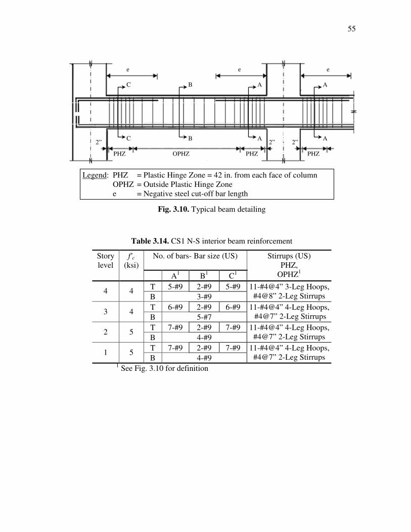
55

e e e

e e e

A

A

A

A

B

BC

C

2” 2” 2”

OPHZPHZ PHZ PHZ

e e e

e e e

A

A

A

A

B

BC

C

2” 2” 2”

OPHZPHZ PHZ PHZ

Fig. 3.10. Typical beam detailing

Table 3.14. CS1 N-S interior beam reinforcement

Story level

f'c

(ksi) No. of bars- Bar size (US)

A1 B1 C1

Stirrups (US) PHZ,

OPHZ1

T 5-#9 2-#9 5-#9 4 4

B 3-#9

11-#4@4” 3-Leg Hoops, #4@8” 2-Leg Stirrups

T 6-#9 2-#9 6-#9 3 4

B 5-#7


T 7-#9 2-#9 7-#9 2 5

B 4-#9


T 7-#9 2-#9 7-#9 1 5

B 4-#9


1 See Fig. 3.10 for definition

Legend: PHZ = Plastic Hinge Zone = 42 in. from each face of column OPHZ = Outside Plastic Hinge Zone e = Negative steel cut-off bar length

56

Table 3.15. CS1 N-S exterior beam reinforcement

Story level

f'c

(ksi) No. of bars- Bar size (US)

A1 B1 C1

Stirrups (US) PHZ,

OPHZ1

T 6-#7 2-#7 6-#7

M 2-#5 4 4

B 4-#7


T 7-#7 2-#7 6-#7

M 2-#5 3 4

B 4-#7


T 5-#9 2-#9 5-#9

M 2-#5 2 5

B 5-#7


T 5-#9 2-#9 5-#9

M 2-#5 1 5

B 5-#7


1 See Fig. 3.10 for more details

Table 3.16. CS1 E-W beam reinforcement

Story level

No. of bars- Bar size (US)

f'c

(ksi) A1 B1 C1

Stirrups (US) PHZ,

OPHZ1

T 4-#7 2-#7 4-#7 4 4

B 4-#5


T 4-#7 2-#7 4-#7 3 4

B 4-#5


T 4-#7 2-#7 4-#7 2 5

B 2-#7/ 2-#5


T 4-#7 2-#7 4-#7 1 5

B 2-#7/ 2-#5



57


No. of bars- Bar size (US) Story level

f’c

(ksi) A1 B1 C1

Stirrups (US) PHZ (Hoops),

OPHZ (Seismic Stirrups)

T 6-#9 2-#9 5-#9 4 4

B 4-#9


T 7-#9 2-#9 6-#9 3 4

B 3-#9/ 2-#7


T 7-#9 2-#9 6-#9 2 4

B 3-#9/ 2-#7


T 7-#9 2-#9 6-#9 1 4

B 3-#9/ 2-#7





f'c

(ksi) A1 B1 C1

Stirrups (US) PHZ,

OPHZ1

T 6-#7 2-#7 6-#7

M 2-#5 4 4

B 4-#7


T 5-#9 2-#9 5-#9

M 2-#5 3 4

B 5-#7


T 5-#9 2-#9 5-#9

M 2-#5 2 4

B 5-#7


T 5-#9 2-#9 5-#9

M 2-#5 1 4

B 5-#7



58



f'c

(ksi) A1 B1 C1

Stirrups (US) PHZ,

OPHZ1

T 3-#7 2-#7 3-#7 4 4

B 4-#5


T 3-#7 2-#7 3-#7 3 4

B 3-#7


T 4-#7 2-#7 4-#7 2 4

B 3-#7


T 4-#7 2-#7 4-#7 1 4

B 3-#7





f’c

(ksi) A1 B1 C1

Stirrups (US) PHZ,

OPHZ1

T 6-#9 2-#9 5-#9 4 4

B 4-#9


T 7-#9 2-#9 6-#9 3 5

B 2-#9/ 4-#7


T 7-#9 2-#9 6-#9 2 5

B 2-#9/ 4-#7


T 7-#9 2-#9 6-#9 1 5

B 2-#9/ 4-#7



59



f’c

(ksi) A1 B1 C1

Stirrups (US) PHZ,

OPHZ1

T 6-#7 2-#7 6-#7

M 2-#5 4 4

B 4-#7


T 5-#9 2-#9 5-#9

M 2-#5 3 5

B 5-#7


T 5-#9 2-#9 5-#9

M 2-#5 2 5

B 5-#7


T 5-#9 2-#9 5-#9

M 2-#5 1 5

B 5-#7





f’c

(ksi) A1 B1 C1

Stirrups (US) PHZ,

OPHZ1

T 3-#7 2-#7 3-#7 4 4

B 3-#7


T 3-#7 2-#7 3-#7 3 5

B 3-#7


T 4-#7 2-#7 4-#7 2 5

B 4-#5


T 4-#7 2-#7 4-#7 1 5

B 4-#5



Two continuous bars must run through the entire beam for the top and bottom

reinforcement. However, the additional negative steel needed near the column face can

be cut-off near the midspan. The number of bars discontinued and the cut off lengths for

CS1, CS2, and CS3 are shown in Tables 3.23 and 3.25.

60

Table 3.23. CS1 negative bar cutoff lengths

Beam location Story level Cut off bars e1 (in.)

1 – 2 5-#9 110

3 4-#9 96 N-S Interior

4 3-#9 74

1 – 3 3-#9 122 N-S Exterior

4 4-#7 96

1 – 3 2-#7 108 E-W

4 1-#7 90 1 See Fig. 3.10 for definition



1 – 3 5-#9 100 N-S Interior

4 4-#9 78

1 – 3 3-#9 106 N-S Exterior

4 4-#7 72

1 – 3 2-#7 66 E-W

4 1-#7 42 1 See Fig. 3.10 for definition



1 – 3 5-#9 105 N-S- Interior

4 4-#9 90

1 – 3 3-#9 92 N-S- Exterior

4 4-#7 68

1 – 2 2-#7 82 E-W

3 – 4 1-#7 75 1 See Fig. 3.10 for definition

Typical PHZ first floor interior and exterior cross sections at the midspan and

column face are shown in Figs. 3.11 and 3.12 for CS1 and CS3 and Figs. 3.13 and 3.14

for CS2. The torsional reinforcement is shown in the exterior beam cross sections.

61

#5 (US) bars #9 (US) bars

5 in.

#4 (US)

hoops

18 in.

21 in.


5 in.

#4 (US)

hoops

18 in.

21 in.


5 in.

#4 (US)

seismic

stirrups

18 in.

21 in.


5 in.

#4 (US)

seismic

stirrups

18 in.

21 in.

(a) Column face (b) Midspan

Fig. 3.11. Typical SMF 1st floor N-S exterior beam cross sections

#4 (US) hoops #9 (US) bars

5 in.

22 in.

16 in.


5 in.

22 in.

16 in.

#4 (US) seismic stirrups #9 (US) bars

5 in.

22 in.

16 in.


5 in.

22 in.

16 in.


Fig. 3.12. Typical SMF 1st floor N-S interior beam cross sections


5 in.

24 in.

16 in.


5 in.

24 in.

16 in.


5 in.

24 in.

16 in.


5 in.

24 in.

16 in.


Fig. 3.13. Typical IMF 1st floor N-S interior beam cross sections

62


5 in.

#3 (US)

hoops

18 in.

21 in.


5 in.

#3 (US)

hoops

18 in.

21 in.


5 in.

#3 (US)

seismic

stirrups

18 in.

21 in.


Fig. 3.14. Typical IMF 1st floor N-S exterior beam cross sections

3.5.3.2 Columns

The column reinforcement for each case study is shown in Fig. 3.15 and Tables

3.26 through 3.28. For the interior columns, the spacing within 24 in. from the joint face

(per ACI 318 Section 21.4.4.4) is given, along with the reinforcement for the remaining

length of the column. The longitudinal column reinforcement was the same for the

columns of the same size. For CS1 and CS3, 12-#8 longitudinal bars provided a

reinforcement ratio, ρ, of 1.4 percent, which is within the allowable range of 1 to 6

percent for SMF structures. The differences in the shear strength reduction factor, φ,

from 0.75 to 0.85 and the load combinations did not have a significant effect. Enough

strength was provided for CS2 by 8-#8 bars for both interior and exterior columns, with

a reinforcement ratio, ρ, of 1.6 percent, as shown in Table 3.27. The interior columns

carried higher axial load, while the exterior columns carried higher moments. The

columns were determined to be non-slender according to ACI 318 Section 10.12.2.

The transverse hoop spacing for CS1 and CS3 was determined by the minimum

cross-sectional area of rectangular hoop reinforcement for SMFs, which depends on

hoop spacing, f’c, and the confinement area in the column. Higher strength concrete

requires smaller transverse hoop spacing. Within the zone where flexural yielding is

likely to occur (24 in. from each joint face as defined by ACI 318), the minimum

transverse spacing was 4 in. for 6000 psi concrete, 5 in. for 5000 psi concrete and 6 in.

63

for 4000 psi concrete. Outside this zone, the minimum spacing increases to 6 in., but was

kept at 5 in. for consistency in the 5000 psi columns. The upper stories did not meet the

strong-column weak-beam requirements; therefore, the flexural yield confinement

reinforcement (#4 bars @ 4 in.) was provided throughout the length of the column per

ACI 318 Section 21.4.2.3. The transverse reinforcement needed for confinement also

provided enough strength for the shear demand. IMF columns have less strict

confinement detailing requirements, and the spacing was increased to 8 in. throughout

the entire column height in CS2.

24 in.

24 in.

12- #8 (US) bars #4 (US) ties

24 in.

24 in.

12- #8 (US) bars

24 in.

24 in.


20 in.

20 in.


20 in.

20 in.


(a) CS1 and CS3 (b) CS2

Fig. 3.15. Column cross-sections

Table 3.26. CS1 column reinforcement

Column location

Story level

No. of bars

Bar size (US) ρ

f’c

(ksi) Tie bar size (US)

and spacing

1 – 2 12-#8 0.014 5 #4@5” Exterior

3 - 4 12-#8 0.014 4 #4@6”

1 – 2 12-#8 0.014 6 7-#4@4”/ #4@6” Interior

3 - 4 12-#8 0.014 5 #4@5”

64


Column location

Story level


ρ

f’c


and spacing

Exterior 1 - 4 8-#8 0.016 4 #3@8”

Interior 1 - 4 8-#8 0.016 4 #3@8”


Column location

Story level


ρ

f’c


and spacing

1 – 3 12-#8 0.014 5 #4@5” Exterior

4 12-#8 0.014 4 #4@4”

1 – 2 12-#8 0.014 6 7-#4@4”/ #4@6”

3 12-#8 0.014 6 #4@4” Interior

4 12-#8 0.014 5 #4@5”

3.5.4 Column-to-Beam Strength Ratios

One of the most important factors in a building’s structural performance under

seismic loading is the column-to-beam strength ratio (Dooley and Bracci 2001). For a

SMF, the column-to-beam strength ratio must be greater than 1.2 according to ACI 318

Section 21.4.2.2 (discussed in Chapter 2). The N-S interior beams control for calculating

the column-to-beam strength ratios to meet this requirement, as they are the strongest

beams. The column-to-beam strength ratios for the first story are summarized in Table

3.29 for use in the performance analysis. The column-to-beam strength ratios are higher

in the E-W direction because the beams are weaker in this direction. For strength

contribution of the beams in the interior frames for CS2 and CS3, the nominal strength

from a single joist was used.

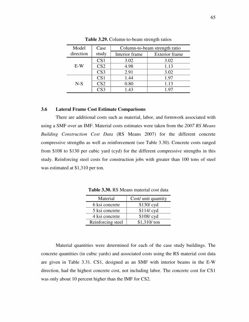
65

Table 3.29. Column-to-beam strength ratios

Column-to-beam strength ratio Model direction

Case study Interior frame Exterior frame

CS1 3.02 3.02

CS2 4.98 1.13 E-W

CS3 2.91 3.02

CS1 1.44 1.97

CS2 0.80 1.13 N-S

CS3 1.43 1.97

3.6 Lateral Frame Cost Estimate Comparisons

There are additional costs such as material, labor, and formwork associated with

using a SMF over an IMF. Material costs estimates were taken from the 2007 RS Means

Building Construction Cost Data (RS Means 2007) for the different concrete

compressive strengths as well as reinforcement (see Table 3.30). Concrete costs ranged

from $108 to $130 per cubic yard (cyd) for the different compressive strengths in this

study. Reinforcing steel costs for construction jobs with greater than 100 tons of steel

was estimated at $1,310 per ton.

Table 3.30. RS Means material cost data

Material Cost/ unit quantity

6 ksi concrete $130/ cyd



Reinforcing steel $1,310/ ton

Material quantities were determined for each of the case study buildings. The

concrete quantities (in cubic yards) and associated costs using the RS material cost data

are given in Table 3.31. CS1, designed as an SMF with interior beams in the E-W

direction, had the highest concrete cost, not including labor. The concrete cost for CS1

was only about 10 percent higher than the IMF for CS2.

66

Since the reinforcement quantities were very similar for the SMF buildings (CS1

and CS3), the comparison only includes CS1 and CS2 (designed as an IMF).

Reinforcement quantities include longitudinal bars and transverse hoops and ties. As

shown in Table 3.32, the SMF buildings had more than twice as much column

reinforcement as the IMF building due to the larger column area and smaller transverse

reinforcement spacing. The beam reinforcement was similar between the two lateral

frame types. The total cost increase for reinforcement quantities, not including

placement, for a SMF versus an IMF was about 15 percent.

Table 3.31. Concrete quantities and costs

Quantity (cyd) Cost f’c

CS1 CS2 CS3 CS1 CS2 CS3

6 ksi 32 - 32 $4,160 - $4,160

5 ksi 811 - 778 $92,450 - $88,690

4 ksi 776 1,501 742 $83,810 $162,110 $80,140

Total 1,619 1,501 1,552 $180,420 $162,110 $172,990

Table 3.32. Reinforcement quantities and costs

Quantity (tons) Cost Location

SMF IMF SMF IMF

Columns 39 18 $51,090 $24,570

Beams 102 101 $133,620 $137,870

Total 141 119 $184,710 $162,440

Some additional structural costs that were not computed include forming and

labor costs, which would vary for the type of lateral system. According to the RS Means

Construction Cost Data (2007), forming can be one of the most expensive costs in

construction. Beams with the same depth as the wide-module joists reduces forming

costs uniformly for each case study; however, there is an additional cost in forming

around the interior E-W beams for CS1, as well as the intersection area of the smaller

67

beams into the columns for the SMF buildings. The additional labor to place the smaller

column tie spacing as well as the greater number of ties within the cross section should

also be taken into consideration.

Professional cost estimates for constructing an ordinary moment frame (OMF)

building and an SMF building were used in a study by Hayes et al. (2005), and the costs

were determined to be 30 percent higher for the SMF. An OMF does not have any

detailing requirements for seismic loading, while an IMF does have some detailing

requirements. The difference in costs for an IMF compared to an SMF should be smaller

than an OMF to an SMF. These costs, however, only include structural costs, which are

generally a small portion of the overall cost of the building. The professional structural

cost estimate in Hayes et al. (2005) was estimated to be about 10 percent of the total

building costs.

68

4 NONLINEAR MODELING

4.1 Introduction

This section presents the modeling procedures for the case study buildings. The

ZEUS-NL program developed by Elnashai et al. (2002) was used for the nonlinear

analysis. The synthetic ground motion records developed by Rix and Fernandez (2006)

for the Memphis, Tennessee, Lowlands for 2% and 10% probabilities of exceedance in

50 years were used in the nonlinear dynamic analysis. The following sections describe

the analytical modeling assumptions and synthetic ground motions.

4.2 Analytical Models

4.2.1 General

ZEUS-NL is a finite element structural analysis program developed for

eigenvalue, push-over, and nonlinear dynamic analysis. The program uses a fiber

element model capable of representing the spread of inelasticity within the member

cross-section and along the member length to model two-dimensional and three-

dimensional steel, reinforced concrete (RC), and composite structures. Effects of

geometric and material nonlinear behavior are taken into account through inelastic cyclic

specified material constitutive relationships. Hueste and Bai (2007), Erbenik and

Elnashai (2004), and Jeong and Elnashai (2005) have also investigated the seismic

vulnerability of RC structures using ZEUS-NL.

The fiber element approach in ZEUS-NL divides the cross section of the material

into individual layers as shown in Fig. 4.1. Each fiber is classified by an appropriate

material stress-strain relationship (Karayannis 1994). The cubic element, used for

modeling members, evaluates the element forces through numerical integration at the

two Gauss points shown in Fig. 4.2.

69

Fig. 4.1. Decomposition of a rectangular RC section (Elnashai et al. 2000)

Fig. 4.2. Degrees of freedom and Gauss points of cubic formulation (Karayannis 1994)

In this study, the constant-average acceleration method (γ=0.5, β=0.25) for the

Newmark integration scheme was used. A time step of 0.005 was used for the dynamic

response history analysis, which matches the time interval for the synthetic ground

motion records.

4.2.2 Building Model

Due to the symmetrical configuration and lack of irregularities, one-half of each

case study structure was modeled as a two-dimensional frame. Both directions (N-S and

E-W) were analyzed in ZEUS-NL to examine effects from the differences in structural

member layout between the case studies. In the long direction (E-W), one exterior and

one interior frame were linked with rigid truss elements that only allow lateral force and

70

displacement transfer between frames. In the short direction (N-S), one exterior and two

interior frames were linked with rigid truss elements. The overall geometry of the frames

modeled in each direction is shown in Fig. 4.3.

Exterior Interior beams

beams (or joists)

(a) E-W direction

Exterior Interior Interior . beams beams beams .

(b) N-S direction

Fig. 4.3. ZEUS-NL 2-D frame models

The effective flange widths for the beams were determined from ACI 318

Section 8.10. Uncracked section properties were used because ZEUS-NL updates the

member properties at each time step interval during the analysis as cracking occurs

under loading. Modeling the 5 in. thick slab without the wide-module pan joists led to

convergence problems in the finite element model. Therefore, single wide-module joists

were included along the E-W interior frames in the CS2 and CS3 models to represent the

additional stiffness contribution of the joists to the lateral system. The actual 6 in. web

Rigid links (typ.)

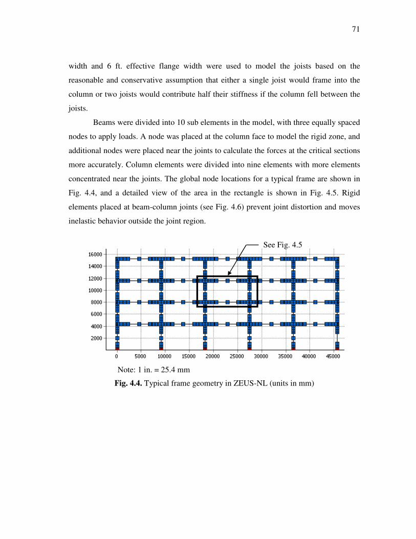
71

width and 6 ft. effective flange width were used to model the joists based on the

reasonable and conservative assumption that either a single joist would frame into the

column or two joists would contribute half their stiffness if the column fell between the

joists.

Beams were divided into 10 sub elements in the model, with three equally spaced

nodes to apply loads. A node was placed at the column face to model the rigid zone, and

additional nodes were placed near the joints to calculate the forces at the critical sections

more accurately. Column elements were divided into nine elements with more elements

concentrated near the joints. The global node locations for a typical frame are shown in

Fig. 4.4, and a detailed view of the area in the rectangle is shown in Fig. 4.5. Rigid

elements placed at beam-column joints (see Fig. 4.6) prevent joint distortion and moves

inelastic behavior outside the joint region.

Note: 1 in. = 25.4 mm

Fig. 4.4. Typical frame geometry in ZEUS-NL (units in mm)

See Fig. 4.5

72

Note: 1 in. = 25.4 mm

Fig. 4.5. Typical node locations for modeling frame members (units in mm)

Fig. 4.6. Rigid joint definition

4.2.3 Individual Member Modeling

The structural members (beams, joists, columns, and rigid connections) were

modeled using a cubic plastic three-dimensional element (cubic). To model the rigid

joints, the joint element (joint) was used. Column cross-sections were defined using the

RC rectangular section (rcrs), and the beam and wide-module joist cross-sections were

defined using the RC T-section (rcts). The rigid joints were modeled with the rectangular

solid section (rss) with high axial stiffness. The ZEUS-NL sections used in this study are

Rigid Joints

Node (typical)

73

shown in Fig. 4.7. To model the reinforcing steel and rigid connections, the bilinear

elasto-plastic material model with kinematic strain hardening (stl1) was used, while the

uniaxial constant confinement concrete material model (conc2) was used to model the

concrete. The material models for stl1 and conc2 are shown in Fig. 4.8.

(a) RC retangular (rcrs) (b) RC flanged (rcts) (c) Rectangular solid (rss)

Fig. 4.7. ZEUS-NL element cross-sections (adapted from Elnashai et al. 2002)

(a) Concrete (con2) (b) Steel (stl1)

Fig. 4.8. ZEUS-NL material models (Elnashai et al. 2002)

74

The stl1 parameters are Young’s modulus (E), yield strength (σy), and a strain-

hardening parameter (µ). Input parameters for the conc2 model include compressive

strength (f’c), tensile strength (ft), maximum strain (εco) and a confinement factor (k). The

material modeling parameters and values are shown in Table 4.1. Confinement factors

are discussed in the following section. The material properties for the rigid connections

had very high values of E and σy to prevent yielding. Three sets of conc2 properties were

used to model the three different concrete compressive strengths.

Table 4.1. ZEUS-NL material modeling parameter values

Material type Parameter Values

E 200,000 N/mm2 (29,000 ksi)

σy 413 N/mm2 (60,000 psi) stl1

(Reinforcing steel) µ 0.02

E 6,890,000 N/mm2 (1,000,000 ksi)

σy 34,500 N/mm2 (5,000,000 psi) stl1

(Rigid connection) µ 0.02

f′c 27.6 N/mm2 (4000 psi)

ft 2.76 N/mm2 (400 psi) conc2

(4 ksi concrete) εco 0.002

f′c 34.5 N/mm2 (5000 psi)



f′c 41.4 N/mm2 (6000 psi)



Note: See Fig. 4.8 for graphical description of variables.

4.2.4 Confinement Factors

ZEUS-NL uses a constant confinement factor, k, to model the effects of

transverse confinement in the members based on the model by Mander et al. (1988).

This factor is dependent on the transverse and longitudinal reinforcement, concrete

75

strength, and member dimensions. The confinement factor provides additional strength

past the initial compressive strength, f’c, and less steep stiffness degradation after the

initiation of yielding in the stress-strain curve in Fig. 4.8. The confinement factor for a

rectangular concrete section with axial compression forces is calculated as the ratio of

the confined concrete compressive strength, f’cc, to the unconfined concrete compressive

strength, f’co, and is calculated using the following equations (Mander et al. 1988).

7.94 ' '' ' 1.254 2.254 1 2

' 'l l

cc co

co co

f ff f

f f

= − + + −

(4.1)

'l e yh

f k fρ= (4.2)

ee

cc

Ak

A= (4.3)

( )2

1

' ' '1 1

6 2 2

ni

e c c

i c c

w s sA b d

b d=

= − − −

∑ (4.4)

( )1cc c ccA A ρ= − (4.5)

where: f’co = Unconfined concrete compressive strength

'lf = Effective lateral confining stresses

ek = Confinement effectiveness coefficient

yhf = Yield strength of transverse reinforcement

eA = Area of effectively confined core concrete

ccA = Area of core within center lines of perimeter spiral or hoops

excluding area of longitudinal steel

cA = Area of core of section within center lines of perimeter spiral

cb = Concrete core dimension to center line of perimeter hoop in x-

direction

cd = Concrete core dimension to center line of perimeter hoop in y-

direction

'iw = ith clear transverse spacing between adjacent longitudinal bars

's = Clear spacing between spiral or hoop bars

ccρ = Ratio of area of longitudinal steel to area of core of section

76

The type of moment frame had the largest effect on the value of k. The SMF case

studies, CS1 and CS3, had confinement factors ranging from 1.27 to 1.43 for the

different f’c values and transverse reinforcement (TR) spacing in the columns as shown

in Table 4.2. The CS2 columns had a smaller k value of 1.12 predominantly due to the

larger TR spacing. These k values applied in both model directions. The beam

confinement factors are shown in Tables 4.3 and 4.4 for the E-W and N-S directions.

The k values changed for the different f’c values, reinforcement, and beam sizes. The N-

S beams were more heavily loaded and reinforced, and correspondingly had higher k

values than the E-W beams. The concrete outside the transverse reinforcement was

considered unconfined with a k equal to 1.0.

Table 4.2. ZEUS-NL column confinement factors

Case study

f’c (ksi)

TR bar size (US) and spacing

Confinement factor, k

4 #4@6” 1.39

5 #4@5” 1.40

6 #4@4” 1.43

CS1 CS3

6 #4@6” 1.27

CS2 4 #3@8” 1.12

Table 4.3. ZEUS-NL beam confinement factors (E-W)

Confinement factor, k Case study

Location f’c

(ksi) Story level Interior Exterior

5 1 – 2 1.16 1.16 PHZ

4 3 – 4 1.21 1.21

5 1 – 2 1.00 1.00 CS1

OPHZ 4 3 – 4 1.00 1.00

PHZ 4 1 – 4 1.12 - CS2

OPHZ 4 1 – 4 1.00 -

5 1 – 3 1.16 - PHZ

4 4 1.21 -

5 1 – 3 1.00 - CS3

OPHZ 4 4 1.00 -

77

Table 4.4. ZEUS-NL beam confinement factors (N-S)

Confinement factor, k Case study

Location f’c

(ksi) Story level Interior Exterior

5 1 – 2 1.33 1.28

4 3 1.40 1.41 PHZ

4 4 1.35 1.41

5 1 – 2 1.10 1.05

4 3 1.10 1.05

CS1

OPHZ

4 4 1.10 1.05

PHZ 4 1 – 4 1.31 1.19 CS2

OPHZ 4 1 – 4 1.14 1.00

5 1 – 3 1.33 1.18 PHZ

4 4 1.40 1.20

5 1 – 3 1.06 1.00 CS3

OPHZ 4 4 1.06 1.00

4.2.5 Loads, Masses and Damping

The gravity loads were applied as point loads to the beams based on the tributary

seismic weight (member self-weight, superimposed dead, and partition loads) using the

approximate load path. ZEUS-NL cannot model distributed loads; therefore, equivalent

point loads based on the concentrated load factors in Table 3-22a of the AISC Steel

Construction Manual (2005) were used for the E-W floor members with a distributed

tributary load, w (see Fig. 4.9). For the N-S beams, the tributary loads from the joists

were applied directly as point loads. In the dynamic analysis, tributary masses were

lumped at the beam-column joints using a lumped mass element (Lmass) to represent the

seismic dead weight.

78

Fig. 4.9. Equivalent point loads applied to E-W members and joists

4.3 Synthetic Ground Motions

Representative strong ground motions for the New Madrid Seismic Zone are not

available due to the lack of recorded strong motion data in this region. Therefore,

synthetic ground motions developed by Rix and Fernandez (2006) for 2% and 10%

probabilities of exceedance in 50 years earthquake scenarios were used in the dynamic

analysis. These ground motions reflect attenuation relationships for soil sites in the

Upper Mississippi Embayment with incorporated effects of epistemic and aleatory

uncertainties in source, path, and site processes, as well as the effect of non-linear soil

behavior. Spectral accelerations for five percent damping for each suite of ten ground

motions are shown in Fig. 4.10. The acceleration time histories are given in Appendix A.

0.0

0.2

0.4

0.6

0.8

1.0

0 1 2 3

Time Period (s)

Sp

ectr

al A

ccel

. (g

)

0.0

0.2

0.4

0.6

0.8

1.0

0 1 2 3

Time Period (s)

Sp

ectr

al A

ccel

. (g

)

(a) 10% in 50 years (b) 2% in 50 years

Fig. 4.10. Spectral accelerations for Rix-Fernandez ground motions

0.103 wL 0.265 wL 0.265 wL 0.265 wL 0.103 wL

L

79

To reduce computational time, the ground motions were truncated at the time

point where the energy reached 95 percent of the total energy. This procedure was based

on recommendations by Trifunac and Brady (1975) that the duration of the strong

ground motion be the time interval remaining between the low and high 5 percent cut-off

of the total energy. The equation to compute the total energy of a strong ground motion

record is given in Eq. (4.6). Tables 4.5 and 4.6 show the ground motion record details.

2

0

( )t

TotalE a t dt=∫ (4.6)

where :

ETotal = Total energy of a ground motion record

a(t) = Acceleration at time, t

Table 4.5. 10% in 50 years Rix-Fernandez ground motions

Ground motion

Peak ground acceleration (g)

Duration (s)

Duration of 95% energy (s)

475_01 0.1565 55.645 47.260

475_02 0.1235 55.390 46.490

475_03 0.1047 58.670 50.500

475_04 0.1309 85.770 74.035

475_05 0.1219 71.660 64.285

475_06 0.1046 71.710 64.320

475_07 0.1610 59.730 51.455

475_08 0.1710 60.095 51.795

475_09 0.1143 43.710 35.840

475_10 0.0975 44.530 37.785

80

Table 4.6. 2% in 50 years Rix-Fernandez ground motions

Ground motion

Peak ground acceleration (g)

Duration (s)

Duration of 95% energy (s)

2475_01 0.3139 55.365 46.200

2475_02 0.3352 54.800 45.320

2475_03 0.2748 58.945 51.970

2475_04 0.3266 84.245 72.615

2475_05 0.2915 73.355 67.145

2475_06 0.3076 72.330 65.670

2475_07 0.3380 59.530 51.540

2475_08 0.3734 57.975 49.400

2475_09 0.3298 43.595 35.045

2475_10 0.3390 43.565 36.815

81

5 ANALYSIS AND EVALUATION

5.1 Nonlinear Analysis

5.1.1 General

The building models were analyzed in both the N-S and E-W directions. The

case studies have the most variation in the E-W direction due to the weaker gravity

designed interior frames in CS2 and CS3. The main distinction in the N-S direction is

between the special (CS1 and CS3) and intermediate (CS2) moment frames. Nonlinear

static push-over analysis was conducted to obtain the overall capacity of each structure.

Nonlinear dynamic response history analysis was also conducted for two sets of

synthetic ground motion records.

5.1.2 Fundamental Periods

ZEUS-NL initially models members using uncracked section properties and

updates the member section properties as cracking occurs under loading according to the

relationships describing the material properties. As a result, the eigenvalue analysis for

each case study produced uncracked fundamental periods. To determine more

representative cracked fundamental periods, the displacement responses were used from

an impulse load of 0.4g corresponding to the maximum peak ground acceleration (PGA)

of the median 2% in 50 years ground motion.

The fundamental periods determined from the ZEUS-NL analysis were compared

to those from the ETABS models with uncracked cracked section properties and cracked

sections properties based on ACI 318 recommendations. The E-W fundamental periods

are summarized in Table 5.1. The CS2 and CS3 ETABS models are more flexible in the

long (E-W) direction because the ETABS models (used for design) only include the

elements designed to resist lateral loads, whereas the ZEUS-NL models (used for

nonlinear analysis) contain all structural members including gravity designed elements.

82

The differences in building stiffness can be seen by comparing the fundamental periods

of each case study.

Table 5.1. Comparison of fundamental periods, T (s) (E-W)

ZEUS-NL ETABS Case Study Cracked Uncracked Cracked Uncracked

CS1 1.27 0.72 1.15 0.77

CS2 1.30 0.96 1.80 1.25

CS3 1.29 0.82 1.48 1.00

The fundamental periods for the ZEUS-NL models in the N-S direction are given

in Table 5.2. The structures are slightly stiffer in this direction, as indicated by the

shorter periods. The smaller columns with a lower f’c in CS2 produced a more flexible

structure and longer periods than CS1 and CS3 in this direction.

Table 5.2. ZEUS-NL fundamental periods, T (s) (N-S)

Case study Cracked Uncracked

CS1 1.13 0.68

CS2 1.25 0.82

CS3 1.08 0.66

5.1.3 Push-over Analysis

Two vertical distributions of lateral loads were used in the static push-over

analysis: a vertical distribution proportional to the fundamental mode shape and a

rectangular uniform distribution (see Fig. 5.1). These load patterns were intended to

produce a lateral response envelope for the structures. The load percentages based on the

first mode shape from the eigenvalue analysis shown in Fig. 5.1(a) vary slightly by case

study and analysis direction. Each modal pattern resembles an inverted triangular shape

and is referred to as the triangular push-over in the following sections. A load control

83

phase was used in the push-over analysis to develop the load deflection curve until

convergence difficulties emerged and the ZEUS-NL analysis automatically switched to a

displacement control phase to capture the post-yield behavior of the structure.

(a) Modal (inverted triangular) pattern (b) Rectangular pattern

Fig. 5.1. Load patterns for push-over analysis

The push-over curves for the E-W direction are shown in Fig. 5.2. The horizontal

axis displays the building drift, defined as the top story displacement divided by the total

building height. The vertical axis is the base shear ratio, V/W, where V is the total base

shear force and W is the seismic weight of the building. The rectangular pattern shows

more strength capacity for each case study than the triangular pattern. In each case, CS1

with interior moment frames, showed greater initial stiffness and strength than CS2 and

CS3. Although CS2 and CS3 had the same interior gravity designed wide-module joists,

the larger columns with special seismic detailing in CS3 exhibited more ductility.

84

0

5

10

15

20

25

30

0 1 2 3 4

Building Drift (%)

V/W

(%

)

CS1CS2CS3

E-W

0

5

10

15

20

25

30

0 1 2 3 4

Building Drift (%)

V/W

(%

)

CS1CS2CS3

E-W

(a) Rectangular push-over (b) Triangular push-over

Fig. 5.2. Push-over results (E-W)

Fig. 5.3 shows the push-over curves for the case studies in the N-S direction. The

similarity in the push-over curves of CS1 and CS3 is due to the same beam and column

sizes in the N-S frames. CS3 had slightly different f’c values and reinforcement, which

may explain the difference in performance past the yield point. The negative slope after

initial yielding in the CS2 push-over curve signifies a soft first story mechanism. The

cut-off points of the CS2 curves corresponds to a strength degradation of twenty percent.

85

0

5

10

15

20

25

30

35

0 1 2 3 4

Building Drift (%)

V/W

(%

) .

CS1

CS2

CS3

N-S

0

5

10

15

20

25

30

35

0 1 2 3 4

Building Drift (%)

V/W

(%

)

CS1

CS2

CS3

N-S

(a) Rectangular push-over (b) Triangular push-over

Fig. 5.3. Push-over results (N-S)

5.1.4 Dynamic Analysis

The nonlinear dynamic analysis was conducted with two suites of synthetic

ground motions developed by Rix and Fernandez (2006) for 2% and 10% probabilities

of exceedance in 50 years hazard levels. Each suite contained 10 ground motions, and

the median response from each ground motions suite was used to compare the case study

responses. The same trends noted for the static analysis were observed when comparing

the case study dynamic response values.

Table 5.3 gives the maximum dynamic response for each case study for the 10%

in 50 years ground motion records in the E-W direction, and Table 5.4 gives the

maximum dynamic response for the 2% in 50 years ground motion records. The median

response is provided in the tables for the median maximum base shear ratio, V/W, and

median maximum building drift for each case study.

86

Table 5.3. E-W maximum building drift and base shear ratio (10% in 50 years)

V/W (%) Max. building drift (%) Ground motion CS1 CS2 CS3 CS1 CS2 CS3

475_01 12.80 11.50 14.78 0.54 0.94 0.96

475_02 13.21 9.61 12.27 0.62 0.56 0.67

475_03 16.44 9.04 15.42 1.22 1.10 1.22

475_04 16.16 9.99 14.47 0.98 1.06 1.15

475_05 12.91 10.38 11.24 0.51 0.59 0.62

475_06 10.38 5.76 10.47 0.34 0.36 0.39

475_07 13.07 7.61 11.04 0.49 0.51 0.50

475_08 15.26 9.76 12.65 0.71 0.63 0.87

475_09 14.43 8.63 12.69 0.60 0.61 0.72

475_10 10.62 7.28 11.83 0.44 0.57 0.60

Median 13.14 9.32 12.46 0.57 0.60 0.69

Table 5.4. E-W maximum building drift and base shear ratio (2% in 50 years)

V/W (%) Max. building drift (%) Ground motion CS1 CS2* CS3 CS1 CS2* CS3

2475_01 19.59 12.79 16.64 2.35 2.34 2.56

2475_02 20.46 16.74 17.83 2.20 1.12 2.94

2475_03 18.50 11.32 16.45 2.85 2.35 3.01

2475_04 21.82 20.90 18.23 6.34 3.09 5.67

2475_05 18.60 13.73 17.89 2.64 2.81 2.53

2475_06 19.04 12.50 16.76 2.67 1.91 2.34

2475_07 21.88 23.53 20.45 1.85 1.33 1.86

2475_08 19.99 12.30 19.78 2.33 1.78 2.92

2475_09 19.07 10.60 18.18 2.47 1.26 2.68

2475_10 20.28 24.75 18.72 3.51 3.59 3.96

Median 19.79 13.26 18.03 2.55 2.13 2.80

*Reported results are values immediately before model became unstable

The median E-W responses for the 10% in 50 years motions show that CS1 had

greater shear demands and lower drifts than CS2 and CS3. The CS3 shear demand was

close to that of CS1, while the CS2 shear demand was significantly lower. For the 2% in

50 years motions, the CS2 nonlinear analysis stopped when the demands exceeded the

capacity of the wide-module joists and large plastic rotation demands occurred leading

87

to instability. Only one of the ten ground motion records ran completely through. The

reported E-W 2% in 50 years results for CS2 are the values computed immediately

before the instabilities. The wide-module joists in CS3 withstood the 2% in 50 years

ground motions without exceeding their capacity, which can be attributed to the higher

ductility and strength in the SMF columns. The 2% in 50 years performance response

showed a similar trend for the case studies to that of the 10% in 50 years response.

However, the wide-module joists exceeded their capacity at lower maximum drifts in

CS2 than the maximum response for CS1 or CS3.

The dynamic results for the 10% in 50 years ground motion records are given in

Table 5.5 for the N-S direction and in Table 5.6 for the 2% in 50 years ground motion

records. As in the push-over analysis, the N-S direction showed greater shear demands

than the E-W direction for each case study.

Table 5.5. N-S maximum building drift and base shear ratio (10% in 50 years)


475_01 15.86 15.63 13.73 0.42 0.68 0.38

475_02 16.44 12.75 16.08 0.46 0.47 0.49

475_03 19.68 16.59 19.76 0.78 0.95 0.66

475_04 20.08 16.03 20.78 0.75 0.78 0.77

475_05 14.39 12.12 16.94 0.42 0.41 0.45

475_06 15.69 10.64 15.89 0.40 0.37 0.48

475_07 17.34 12.16 17.67 0.53 0.49 0.52

475_08 20.58 14.47 21.01 0.77 0.61 0.75

475_09 19.27 14.12 20.49 0.69 0.59 0.79

475_10 18.83 11.05 15.69 0.59 0.34 0.44

Median 18.08 13.43 17.31 0.56 0.54 0.50

88

Table 5.6. N-S maximum building drift and base shear ratio (2% in 50 years)


2475_01 26.64 17.04 25.24 1.96 1.62 1.48

2475_02 26.22 16.79 26.87 2.69 2.27 2.25

2475_03 25.87 16.51 27.55 2.07 1.95 1.91

2475_04 28.43 17.39 28.43 3.14 7.75 2.31

2475_05 26.84 16.55 27.52 2.96 3.00 1.77

2475_06 27.87 16.47 27.78 2.12 2.61 1.85

2475_07 25.78 16.47 25.16 1.55 1.41 1.45

2475_08 25.66 17.02 28.21 3.30 2.89 3.02

2475_09 25.85 16.90 26.22 1.46 2.08 1.38

2475_10 26.08 17.01 26.15 1.48 4.87 1.33

Median 26.15 16.85 27.20 2.10 2.44 1.81

With moment frames along each bay in the N-S direction, the ground motion

records ran completely in the CS2 2% in 50 years analysis and can be more directly

compared with the other case studies. The N-S 10% in 50 years median responses were

similar to the E-W direction. For the 2% in 50 years median response, however, CS3

showed slightly higher median base shear demands and lower drifts than CS1.

5.1.5 Comparison of Push-over and Dynamic Results

The push-over response curves along with the maximum dynamic responses for

each ground motion for the E-W direction are provided in Fig. 5.4. Each discrete data

point represents the maximum dynamic response (maximum base shear and the

maximum building drift) for a ground motion record. The median ground motion

responses for both the 10% and 2% in 50 years motions are circled in each of the figures.

The legend for CS1 in Fig. 5.4. also applies to CS2 and CS3.

89

0

5

10

15

20

25

30

0 1 2 3 4Building Drift (%)

V/W

(%

)

10% in 50 Rect.2% in 50 Tri.

Dynamic Push-over

EW

(a) CS1

0

5

10

15

20

25

30

0 1 2 3 4

Building Drift (%)

V/W

(%

)

EW

(b) CS2

0

5

10

15

20

25

30


V/W

(%

)

EW

(c) CS3

Fig. 5.4. Comparison of push-over and dynamic analyses (E-W)

90

The dynamic results generally fell between the triangular and rectangular push-

over curves, giving an approximate envelope of the structural response. While the CS3

push-over curve in the E-W direction showed a similar initial trend to CS2, the dynamic

results indicated that with stronger columns and special seismic detailing, CS3 actually

had additional lateral resistance for a given drift demand under earthquake loading.

In the N-S direction, the dynamic response is more consistent with the static

response. Fig. 5.5 shows the comparison of the push-over curves in the N-S direction

with the maximum dynamic response for each of the twenty ground motion records. The

push-over analysis shows a story mechanism forming in the N-S direction for CS2, but

the dynamic results do not follow the strength reduction observed in the push-over

analysis. For this particular structure, the maximum drift response for the 2% in 50 years

hazard occurred at lower shear values following the story mechanism, while the

maximum shear occurred directly before the story mechanism occurred. This is not

shown in the plots of maximum drift versus maximum base shear, but would be reflected

by a plot of maximum drift versus the corresponding base shear.

91

0

5

10

15

20

25

30

35


V/W

(%

)

10% in 50 Rect.2% in 50 Tri.

N-S

Dynamic Push-over

(a) CS1

0

5

10

15

20

25

30

35


V/W

(%

)

N-S

(b) CS2

0

5

10

15

20

25

30

35

0 1 2 3 4

Building Drift (%)

V/W

(%

)

N-S

(c) CS3

Fig. 5.5. Comparison of push-over and dynamic analyses (N-S)

92

5.2 Performance Evaluation

5.2.1 General

The structural performance criteria provided in FEMA 356 (ASCE 2000) were

used for both global-level and member-level evaluations of the case study buildings.

FEMA 356 provides suggested interstory drift values as a guideline for assessing global

structural performance, while recommended plastic rotation limits specify criteria for

more detailed member-level evaluations.

FEMA 356 safety objectives are designated to meet a target performance level at

a specific hazard level. Performance levels are used to describe the maximum damage to

a structure. The performance levels included in this study are Life Safety (LS) and

Collapse Prevention (CP). LS performance is defined as significant damage has occurred,

but there is still some margin against structural collapse. CP performance is when a

structure does not have a margin against collapse after an earthquake and can just barely

support gravity loads. The Basic Safety Objective (BSO) suggested by FEMA 356 is LS

performance for the 10% in 50 years hazard level and CP performance for the 2% in 50

years hazard level. Meeting either of these performances without the other is considered

a Limited Objective.

5.2.2 Global-level Limits

5.2.2.1 General

FEMA 356 suggests a typical value of 2% interstory drift associated with LS

performance level and 4% drift for CP performance for concrete frames. These drift

values are suggested for structures that are properly designed for seismic loadings, such

as SMFs. The IMF case study, with a column-to-beam strength ratio of less than 0.8,

would not necessarily qualify. Ramamoorthy et al. (2006) proposed using reduced

interstory drift values of 1% and 2% interstory drift for the LS and CP performance

levels, respectively, for buildings with insufficient column strength and section detailing,

based on the FEMA 356 member-level rotations. These interstory drift limits (see Table

93

5.7) were compared to the maximum interstory drifts from the ZEUS-NL response

history analysis using the median ground motion records for both hazard levels, shown

in Appendix B.

Table 5.7. Global interstory drift values for concrete frame elements

Drift (%) Structural performance level CS1 CS2 CS3

Life Safety (LS) 2 1 2

Collapse Prevention (CP) 4 2 4

5.2.2.2 E-W Direction

A comparison of the E-W maximum interstory drifts for the median 2% and 10%

in 50 years ground motions with the global drift limits is shown in Fig. 5.6. The median

maximum interstory drifts for the 10% in 50 years hazard were less than 1% for each

case study, meeting both the suggested FEMA 356 2% drift value as well as the

modified 1% drift value for LS performance. The CP drift value of 4% was also met for

the CS1 and CS3 2% in 50 years response.

The dynamic analysis for the CS2 model using the median 2% in 50 years

motion did not complete due to model instability when the capacities of the wide-module

joists were exceeded and large plastic rotations occurred. The response of the building

prior to the instability did not meet the modified CP drift value of 2%. Because the

analysis was not completed for the entire 2% in 50 years ground motion record, the CS2

response is denoted by a dotted line in Fig. 5.6. CS1 and CS3 met both the LS and CP

global drift values for the respective hazard levels, satisfying the BSO for the global

response evaluation, while CS2 only met the limited performance objective of LS for the

10% in 50 years hazard.

94

CPLS

0

1

2

3

4

5

0 1 2 3

Sto

ry L

evel

CS2

10%

in 50

2% in 50

IMF response

CP LS

0 1 2 3 4 5

CS1 CS3

10% in 50

2% in 50

SMF response

Fig. 5.6. Median maximum interstory drifts (E-W)

5.2.2.3 N-S Direction

Fig. 5.7 shows the maximum interstory drifts for the median 2% and 10% in 50

years ground motions for the N-S frames, along with the FEMA 356 global drift values.

The median 10% in 50 years maximum interstory drifts were also less than 1% for each

case study in the N-S direction, achieving LS performance for all case studies. The story

mechanism that formed at the first story of CS2 resulted in a predicted maximum median

interstory drift of more than 7%, exceeding the CP performance limit. However, the

median maximum interstory drifts were less than 3% for CS1 and CS3, and satisfied the

suggested 4% CP drift value for well-detailed RC frames. The N-S global results

matched the E-W results for the BSO evaluation with only CS2 not satisfying CP

performance for the 2% in 50 years hazard.

Interstory Drift (%)

95

CPLS

0

1

2

3

4

5

0 1 2 3

Sto

ry L

evel

CS2

10%

in 502% in 50

IMF response

Drifts due

to story

mechanism:

> 7%

CP LS

0 1 2 3 4 5

CS1 CS3

10% in 50

2% in 50

SMF response

Fig. 5.7. Median maximum interstory drifts (N-S)

5.2.3 Member-level Limits

5.2.3.1 General

The FEMA 356 member-level evaluation is based on plastic rotation limits for

RC moment frames. This more detailed evaluation uses rotation acceptance criteria

determined for the LS and CP performance levels based on member reinforcement ratios,

confinement, and shear demand-to-strength ratios for beam and columns controlled by

flexure. The ZEUS-NL plastic rotations for the ground motion record nearest the median

response for each story were used in the evaluation. Plastic rotation, θp, is determined as

the inelastic rotation beyond the yield rotation. The yield rotation is based on the

moment-area theorem. The following expressions are used to determine these values.

maxp yθ θ θ= − (5.1)

6

y

y

c cr

M L

E Iθ = (5.2)

where: θp = Plastic rotation (rad.) θmax = Maximum rotation (rad.)


96

θy = Yield rotation (rad.) My = Design moment (kip-in.) Ec = Modulus of elasticity of concrete (ksi) Icr = Cracked section moment of inertia (in.4) L = Length of member (in.)

FEMA 356 has stricter acceptance criteria for members with poor seismic

detailing based on the transverse reinforcement (TR) spacing. If the plastic hinge zone

TR spacing is less than d/3 (where d is the effective member depth) and the strength

provided by the hoops is at least three-fourths of the design shear, then the member is

considered conforming (C). If a member does not meet this classification, it is

nonconforming (NC) with significantly smaller rotation limits for each limit state.

Members are also classified as primary or secondary for rotation acceptance

limits. The main lateral resisting elements such as the moment frame beams and columns

are primary elements, whereas the interior gravity designed wide-module joists are

secondary elements. Secondary elements have larger rotation limits than elements

originally designed for lateral resistance, although the increase is usually offset if the

members are also nonconforming.

5.2.3.2 E-W Direction

The FEMA 356 plastic rotation limits are summarized in Tables 5.8 through 5.10

for the columns and exterior and interior floor members in the E-W frames. These tables

also contain the median maximum plastic rotation for each case study and story level for

both the 10% and 2% in 50 years hazards. The bolded rotations exceeded the

corresponding limit state member rotation limits, and the CS2 rotations in italics were

the last computed values before the model became unstable. The column rotation limits

depended on the TR spacing, f’c and the axial load. The CS2 columns were classified as

NC due to the larger TR spacing, with smaller rotation limits than the CS1 and CS3

limits. The interior wide-module joists in CS2 and CS3 were also classified as NC;

however, as secondary members, the rotation limits were not always lower than the CS1

moment frame interior floor member limits.

97

Table 5.8. Column plastic rotations (E-W)

FEMA 356 limit (rad.) Max. plastic rot. (rad.) Case study

Story level

TR

LS CP 10% in 50 yrs 2% in 50 yrs

1 C 0.0150 0.0200 0.0060 0.0334 2 C 0.0150 0.0200 0.0062 0.0273 3 C 0.0150 0.0200 0.0054 0.0242

CS1

4 C 0.0150 0.0200 0.0050 0.0223

1 NC 0.0031 0.0041 0.0074 0.0784

2 NC 0.0038 0.0048 0.0067 0.0319

3 NC 0.0046 0.0056 0.0063 0.0259 CS2

4 NC 0.0050 0.0060 0.0034 0.0186

1 C 0.0150 0.0200 0.0068 0.0401 2 C 0.0150 0.0200 0.0064 0.0390 3 C 0.0150 0.0204 0.0055 0.0336

CS3

4 C 0.0150 0.0200 0.0052 0.0306 Note: 1. Rotation in bold exceeded the corresponding limit state limits

2. Rotations in italics were the last computed values before the model became unstable

Table 5.9. Exterior frame floor member plastic rotations (E-W)


Story level

TR


1 C 0.0190 0.0247 0.0036 0.0334 2 C 0.0190 0.0247 0.0027 0.0273 3 C 0.0188 0.0247 0.0013 0.0242

CS1

4 C 0.0188 0.0247 0.0004 0.0223

1 C 0.0187 0.0244 0.0040 0.0249 2 C 0.0187 0.0244 0.0027 0.0197

3 C 0.0200 0.0250 0.0013 0.0155 CS2

4 C 0.0200 0.0250 0.0004 0.0091

1 C 0.0190 0.0245 0.0047 0.0274 2 C 0.0190 0.0245 0.0032 0.0292 3 C 0.0190 0.0245 0.0036 0.0216

CS3

4 C 0.0188 0.0244 0.0027 0.0216

98

Table 5.10. Interior frame floor member plastic rotations (E-W)


Story level

TR


1 C 0.0193 0.0247 0.0050 0.0262 2 C 0.0193 0.0247 0.0045 0.0280 3 C 0.0194 0.0247 0.0036 0.0257

CS1

4 C 0.0194 0.0247 0.0026 0.0235

1 NC 0.0180 0.0271 0.0041 0.0733

2 NC 0.0180 0.0271 0.0037 0.0273

3 NC 0.0180 0.0271 0.0030 0.0226 CS2

4 NC 0.0180 0.0271 0.0000 0.0157

1 NC 0.0171 0.0257 0.0024 0.0357 2 NC 0.0171 0.0257 0.0014 0.0342 3 NC 0.0171 0.0257 0.0005 0.0190

CS3

4 NC 0.0160 0.0240 0.0000 0.0169

For the 10% in 50 years hazard, the CS1 and CS3 median maximum response

values were within the beam and column plastic rotation limits for LS performance.

However, CS2 did not meet the stricter NC column rotation limits for LS performance

for the 10% in 50 years ground motions. The locations in CS2 where the column LS

performance limits were exceeded for the median 10% in 50 years motion are shown in

Fig. 5.8.

Fig. 5.8. Locations where LS plastic rotation limits are exceeded in CS2 (E-W)

= Exceedance of plastic rotation limit

Exterior frame Interior frame

99

All the case studies exceeded the CP performance level for the 2% in 50 years

motions; however, the degree of exceedance varied significantly between the SMF and

IMF buildings. The column plastic rotations of the SMF case studies were at most twice

as large as the corresponding CP rotation limits, compared to up to 18 times the CP

limits for the CS2 columns. As a result, none of the case studies met the BSO in the E-W

direction, and only CS1 and CS3 met the LS limited performance objective. Fig. 5.9

shows the locations where the CP rotation limits were exceeded for the median 2% in 50

years ground motion in each of the case studies.

(a) CS1

(b) CS2

(c) CS3

Fig. 5.9. Locations where CP plastic rotation limits are exceeded (E-W)


100

5.2.3.3 N-S Direction

The N-S evaluation produced similar results to the E-W direction. However,

there were fewer instances of plastic rotation limits being exceeded, indicating that the

E-W direction is more vulnerable. Tables 5.11 through 5.13 give FEMA 356 plastic

rotation limits and the median maximum plastic rotations for each suite of ground

motions in the N-S direction. The column rotation limits were the same as in the E-W

direction, and similarly the only LS plastic rotation limits exceeded for the 10% in 50

years hazard were the CS2 column rotations shown in Fig. 5.10.

Table 5.11. Column plastic rotations (N-S)


Story level

TR


1 C 0.0150 0.0200 0.0063 0.0340 2 C 0.0150 0.0200 0.0052 0.0248 3 C 0.0150 0.0200 0.0044 0.0192

CS1

4 C 0.0150 0.0200 0.0040 0.0149

1 NC 0.0031 0.0041 0.0058 0.0303 2 NC 0.0038 0.0048 0.0051 0.0122 3 NC 0.0046 0.0056 0.0031 0.0062

CS2

4 NC 0.0050 0.0060 0.0028 0.0060 1 C 0.0150 0.0200 0.0058 0.0301 2 C 0.0150 0.0200 0.0046 0.0239 3 C 0.0150 0.0204 0.0032 0.0158

CS3

4 C 0.0150 0.0200 0.0029 0.0102 Note: Rotation in bold exceeded the corresponding performance limits

101

Table 5.12. Exterior frame floor member plastic rotations (N-S)


Story level

TR


1 C 0.0183 0.0241 0.0012 0.0308 2 C 0.0183 0.0241 0.0006 0.0223

3 C 0.0189 0.0244 0.0030 0.0143 CS1

4 C 0.0194 0.0247 0.0022 0.0088

1 C 0.0153 0.0226 0.0014 0.0265 2 C 0.0153 0.0226 0.0003 0.0074

3 C 0.0153 0.0226 0.0000 0.0011 CS2

4 C 0.0168 0.0234 0.0000 0.0023

1 C 0.0148 0.0223 0.0010 0.0253 2 C 0.0148 0.0223 0.0000 0.0194

3 C 0.0148 0.0223 0.0000 0.0150 CS3

4 C 0.0164 0.0231 0.0000 0.0085

Table 5.13. Interior frame floor member plastic rotations (N-S)


Story level

TR


1 C 0.0162 0.0232 0.0024 0.0268 2 C 0.0168 0.0232 0.0011 0.0206

3 C 0.0163 0.0228 0.0003 0.0153 CS1

4 C 0.0169 0.0233 0.0000 0.0108

1 C 0.0138 0.0217 0.0033 0.0224 2 C 0.0138 0.0217 0.0006 0.0065

3 C 0.0138 0.0217 0.0000 0.0020 CS2

4 C 0.0152 0.0225 0.0000 0.0016

1 C 0.0131 0.0211 0.0014 0.0256 2 C 0.0131 0.0211 0.0004 0.0186

3 C 0.0131 0.0211 0.0000 0.0110 CS3

4 C 0.0125 0.0208 0.0000 0.0054

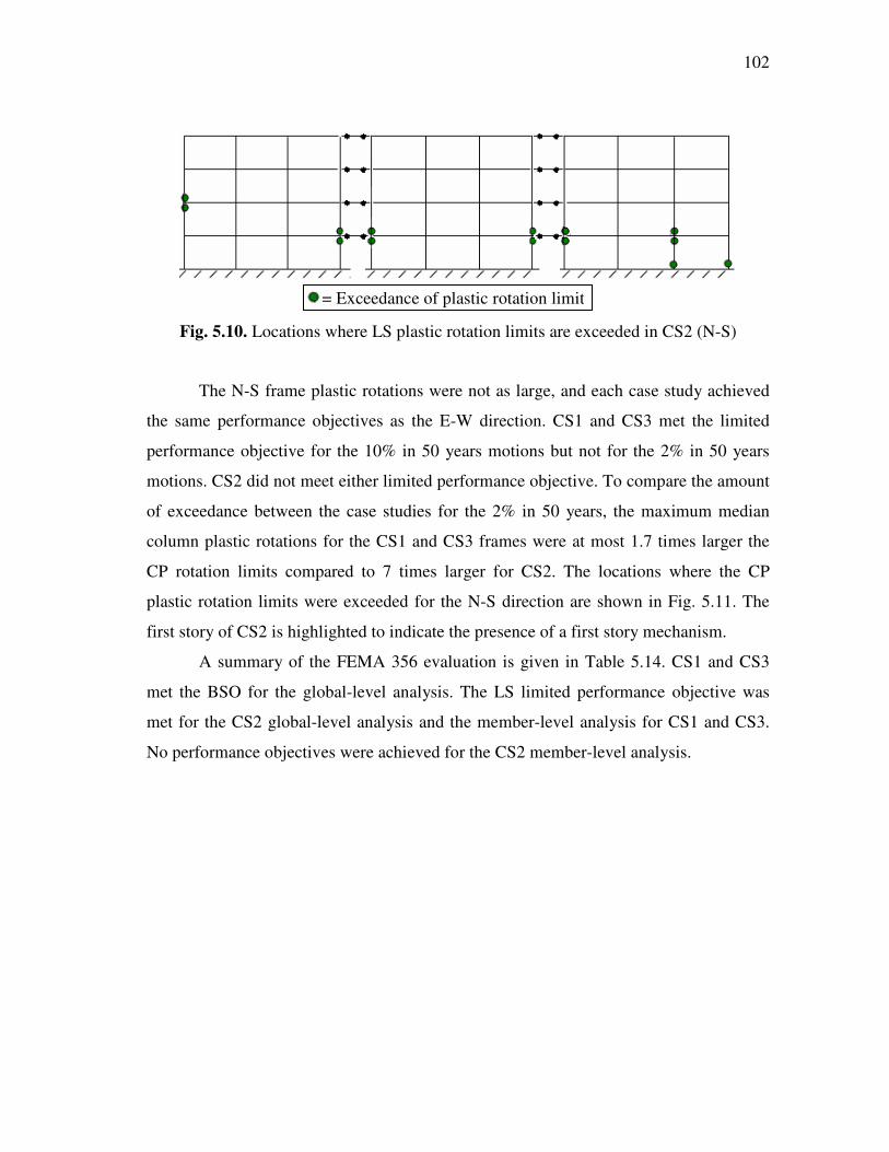
102

Fig. 5.10. Locations where LS plastic rotation limits are exceeded in CS2 (N-S)

The N-S frame plastic rotations were not as large, and each case study achieved

the same performance objectives as the E-W direction. CS1 and CS3 met the limited

performance objective for the 10% in 50 years motions but not for the 2% in 50 years

motions. CS2 did not meet either limited performance objective. To compare the amount

of exceedance between the case studies for the 2% in 50 years, the maximum median

column plastic rotations for the CS1 and CS3 frames were at most 1.7 times larger the

CP rotation limits compared to 7 times larger for CS2. The locations where the CP

plastic rotation limits were exceeded for the N-S direction are shown in Fig. 5.11. The

first story of CS2 is highlighted to indicate the presence of a first story mechanism.

A summary of the FEMA 356 evaluation is given in Table 5.14. CS1 and CS3

met the BSO for the global-level analysis. The LS limited performance objective was

met for the CS2 global-level analysis and the member-level analysis for CS1 and CS3.

No performance objectives were achieved for the CS2 member-level analysis.


103

(a) CS1

(b) CS2

(c) CS3

Fig. 5.11. Locations where CP plastic rotation limits are exceeded (N-S)

Table 5.14. FEMA 356 BSO evaluation for global and member-level performance

Global-level evaluation Member-level evaluation Case study LS

10% in 50 CP

2% in 50 BSO LS

10% in 50 CP

2% in 50 BSO

CS1 O.K. O.K. O.K. O.K. N.G. N.G.

CS2 O.K. N.G. N.G. N.G. N.G. N.G.

CS3 O.K. O.K. O.K. O.K. N.G. N.G.

Key: O.K. = Case study meets performance objective N.G. = Case study does not meet performance objective


104

6 FRAGILITY ANALYSIS

6.1 Introduction

6.1.1 Methodology

Fragility curves were developed to compare the vulnerability of the case study

buildings for varying seismic intensities. The method outlined by Wen et al. (2004) and

summarized in Section 2 was used to develop the fragility curves based on seismic

demands, capacities, and their corresponding uncertainties.

In this study, the seismic demand was determined from the results of the dynamic

analysis with 2% and 10% in 50 years Memphis, Tennessee, ground motions. The

structural capacity was defined as the maximum interstory drift that a member or story

can withstand without reaching a prescribed limit state. The qualitative performance

levels used in this study are taken from the FEMA 356 performance objectives. Along

with the Life Safety (LS) and Collapse Prevention (CP) performance levels from the

earlier FEMA 356 evaluation, the fragility analysis also included the Immediate

Occupancy (IO) performance level. The IO performance level is defined as very minimal

damage such that the building is operational immediately after an earthquake.

Quantitative limit states suggested by Wen et al. (2004) were also used to define

additional structural capacity limits.

The following equation was used to develop the fragility relationships (Wen et al.

2004):

|

2 2 2

|

( | ) 1 a

a

CL D S

a

D S CL M

P LS Sλ λ

β β β

+ = − Φ + +

(6.1)

where: P(LS | Sa) = Probability of exceeding a limit state given the spectral

acceleration at the fundamental period of the building Φ = Standard normal cumulative distribution function

105

CLλ = ln(median drift capacity for a particular limit state), where

drift capacity is expressed as a percentage of the story height

aD Sλ = ln(calculated median demand drift given the spectral

acceleration), where demand drift is determined from a fitted power law equation

aD Sβ = Uncertainty associated with the fitted power law equation

used to estimate demand drift = 2ln(1 )s+

CLβ = Uncertainty associated with the drift capacity criteria, taken

as 0.3 for this study (Wen et al. 2004)

Mβ = Uncertainty associated with analytical modeling of the

structure, taken as 0.3 for this study (Wen et al. 2004)

2s = Square of the standard error =

2

ln( ) ln( )

2

i pY Y

n

− −

∑

iY , pY = Observed demand drift and power law predicted demand

drift, respectively, given the spectral acceleration n = Number of sample data points for demand

6.1.2 Additional Ground Motions

To cover a broader range of seismic demand, the results from an additional

twenty ground motions for Memphis, Tennessee, developed by Wen and Wu (2000) for

2% and 10% probabilities of exceedance in 50 years, were used to define the demand

relationships. Tables 6.1 and 6.2 give the details of these ground motions, and spectral

accelerations with five percent damping are shown in Fig. 6.1 for each suite. The same

method by Trifunac and Brady (1975) was used to truncate the ground motions to 95

percent of the total energy imparted (see Section 4.3). The acceleration time histories are

given in Appendix A.

106

Table 6.1. 10% in 50 years ground motions (Wen and Wu 2000)

Ground motion

PGA

(g)

Duration

(s)

Duration of 95% energy

(s)

Body- wave

magnitude

Focal depth

(mi.)

Epicentral distance

from Memphis (mi.)

475_01wu 0.059 41.0 22.2 6.3 3.2 75

475_02wu 0.075 41.0 19.7 6.4 4.2 36

475_03wu 0.070 41.0 17.5 6.8 11.2 78

475_04wu 0.068 41.0 23.4 6.8 1.3 57

475_05wu 0.108 41.0 14.9 6.2 16.8 66

475_06wu 0.054 150 48.9 6.2 2.0 26

475_07wu 0.070 41.0 20.3 6.5 7.1 37

475_08wu 0.088 20.5 12.4 6.5 14.9 80

475_09wu 0.093 20.5 10.2 6.3 5.9 103

475_10wu 0.064 41.0 18.5 6.8 5.4 22

Table 6.2. 2% in 50 years ground motions (Wen and Wu 2000)

Ground motion

PGA

(g)

Duration

(s)

Duration of 95% energy

(s)

Body- wave

magnitude

Focal depth

(mi.)

Epicentral distance

from Memphis (mi.)

2475_01wu 0.439 150 29.2 8.0 15.9 92

2475_02wu 0.333 150 23.5 8.0 21.1 116

2475_03wu 0.360 150 23.7 8.0 15.9 101

2475_04wu 0.323 150 52.8 8.0 5.7 106

2475_05wu 0.476 150 36.2 8.0 5.7 61

2475_06wu 0.416 150 37.1 8.0 10.8 73

2475_07wu 0.365 150 24.8 8.0 10.8 74

2475_08wu 0.292 150 20.9 8.0 5.7 91

2475_09wu 0.335 150 26.0 8.0 5.7 106

2475_10wu 0.412 150 22.2 8.0 10.8 117

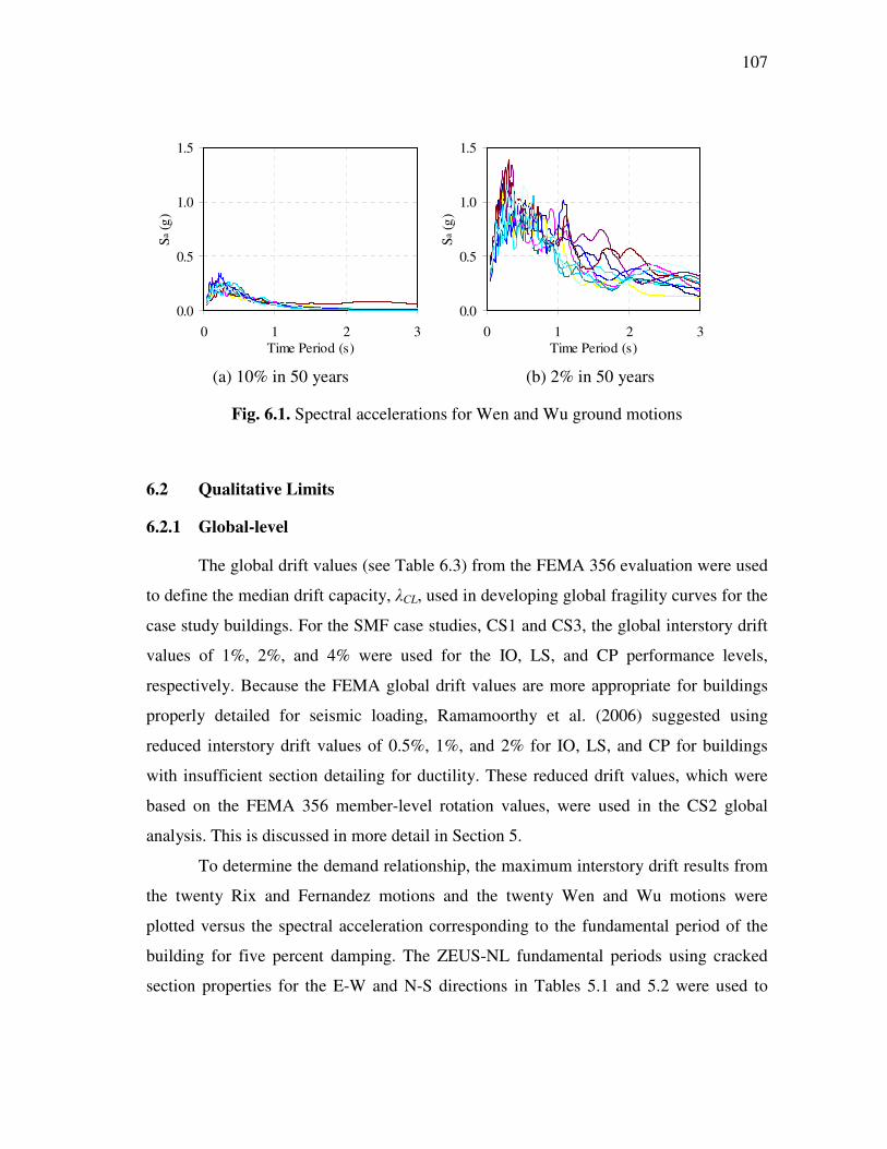
107

0.0

0.5

1.0

1.5

0 1 2 3Time Period (s)

Sa

(g)

0.0

0.5

1.0

1.5

0 1 2 3Time Period (s)

Sa

(g)

(a) 10% in 50 years (b) 2% in 50 years

Fig. 6.1. Spectral accelerations for Wen and Wu ground motions

6.2 Qualitative Limits

6.2.1 Global-level

The global drift values (see Table 6.3) from the FEMA 356 evaluation were used

to define the median drift capacity, λCL, used in developing global fragility curves for the

case study buildings. For the SMF case studies, CS1 and CS3, the global interstory drift

values of 1%, 2%, and 4% were used for the IO, LS, and CP performance levels,

respectively. Because the FEMA global drift values are more appropriate for buildings

properly detailed for seismic loading, Ramamoorthy et al. (2006) suggested using

reduced interstory drift values of 0.5%, 1%, and 2% for IO, LS, and CP for buildings

with insufficient section detailing for ductility. These reduced drift values, which were

based on the FEMA 356 member-level rotation values, were used in the CS2 global

analysis. This is discussed in more detail in Section 5.

To determine the demand relationship, the maximum interstory drift results from

the twenty Rix and Fernandez motions and the twenty Wen and Wu motions were

plotted versus the spectral acceleration corresponding to the fundamental period of the

building for five percent damping. The ZEUS-NL fundamental periods using cracked

section properties for the E-W and N-S directions in Tables 5.1 and 5.2 were used to

108

determine the spectral accelerations corresponding to each ground motion record. A

power law equation was fitted to the forty data points for each case study and direction.

Maximum interstory drifts were used for the controlling story for each ground motion

record in the global fragility analysis. These interstory drifts can be found in Appendix B.

The best fit power equations for the global fragilities are shown in Fig. 6.2 for the E-W

direction and Fig. 6.3 for the N-S direction.

Table 6.3. Global interstory drift limits

Drift (%) Structural performance level

CS1 CS2 CS3

Immediate Occupancy (IO) 1 0.5 1

Life Safety (LS) 2 1 2

Collapse Prevention (CP) 4 2 4

109

y = 4.1287x0.8445

R2 = 0.8252

0

1

2

3

4

5

6

7

8

0.0 0.2 0.4 0.6 0.8 1.0

Sa (g)

Max

. In

ters

tory

Dri

ft (

%)

.

y = 6.3535x0.8812

R2 = 0.7756

0

1

2

3

4

5

6

7

8

0.0 0.2 0.4 0.6 0.8 1.0

Sa (g)

Max

. In

ters

tory

Dri

ft (

%)

.

(a) CS1 (b) CS2

y = 4.8754x0.8316

R2 = 0.8598

0

1

2

3

4

5

6

7

8

0.0 0.2 0.4 0.6 0.8 1.0Sa (g)

Max

. In

ters

tory

Dri

ft (

%)

.

(c) CS3

Fig. 6.2. Development of global power law equations (E-W)

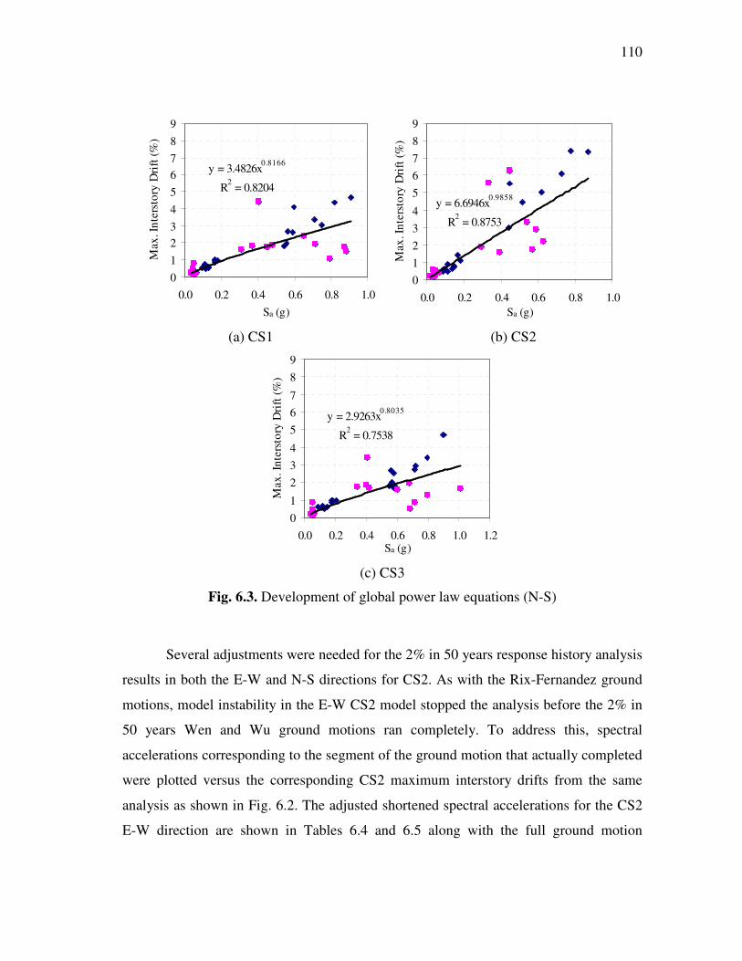
110

y = 3.4826x0.8166

R2 = 0.8204

0

1

2

3

4

5

6

7

8

9

0.0 0.2 0.4 0.6 0.8 1.0

Sa (g)

Max

. In

ters

tory

Dri

ft (

%)

y = 6.6946x0.9858

R2 = 0.8753

0

1

2

3

4

5

6

7

8

9

0.0 0.2 0.4 0.6 0.8 1.0

Sa (g)

Max

. In

ters

tory

Dri

ft (

%)

(a) CS1 (b) CS2

y = 2.9263x0.8035

R2 = 0.7538

0

1

2

3

4

5

6

7

8

9

0.0 0.2 0.4 0.6 0.8 1.0 1.2Sa (g)

Max

. In

ters

tory

Dri

ft (

%)

(c) CS3

Fig. 6.3. Development of global power law equations (N-S)

Several adjustments were needed for the 2% in 50 years response history analysis

results in both the E-W and N-S directions for CS2. As with the Rix-Fernandez ground

motions, model instability in the E-W CS2 model stopped the analysis before the 2% in

50 years Wen and Wu ground motions ran completely. To address this, spectral

accelerations corresponding to the segment of the ground motion that actually completed

were plotted versus the corresponding CS2 maximum interstory drifts from the same

analysis as shown in Fig. 6.2. The adjusted shortened spectral accelerations for the CS2

E-W direction are shown in Tables 6.4 and 6.5 along with the full ground motion

111

spectral accelerations for comparison. Only one 2% in 50 years ground motion fully

completed, and the remaining ground motions completed 30 to 95 percent of the original

duration. Such adjustments were not needed in the N-S direction.

Table 6.4. Reduced 2% in 50 years Wen and Wu motions (CS2 E-W model)

Ground motion

Completed time (s)

Total time (s)

Percent complete

Shortened Sa (g)

Complete Sa (g)

475_01wu 11.65 29.20 39.9 0.132 0.493

475_02wu 19.59 23.44 83.6 0.243 0.395

475_03wu 22.16 23.68 93.6 0.240 0.240

475_04wu 12.68 52.76 24.0 0.240 0.434

475_05wu 15.34 36.20 42.4 0.280 0.676

475_06wu 18.01 37.10 48.5 0.445 0.444

475_07wu 16.25 24.80 65.5 0.267 0.355

475_08wu 15.91 20.90 76.1 0.347 0.592

475_09wu 14.93 26.00 57.4 0.218 0.338

475_10wu 13.41 22.20 60.4 0.241 0.259

Table 6.5. Reduced 2% in 50 years Rix-Fernandez motions (CS2 E-W model)

Ground motion

Completed time (s)

Total time (s)

Percent complete

Shortened Sa (g)

Complete Sa (g)

2475_01wu 46.20 46.20 100.0 0.545 0.550

2475_02wu 34.52 45.32 76.2 0.256 0.672

2475_03wu 48.22 51.97 92.8 0.591 0.591

2475_04wu 46.16 72.62 63.6 0.267 0.743

2475_05wu 66.34 67.14 98.8 0.282 0.596

2475_06wu 47.21 65.67 71.9 0.737 0.737

2475_07wu 34.04 51.54 66.0 0.445 0.445

2475_08wu 32.05 49.40 64.9 0.397 0.832

2475_09wu 16.15 35.05 46.1 0.295 0.472

2475_10wu 15.56 36.81 42.3 0.282 0.481

In addition, the CS2 story mechanism in the N-S direction for the 2% in 50 years

motions caused excessive first story drifts in the ZEUS-NL analysis that were out of the

112

range of reasonable structural performance. For the fitted power equation relationship, a

cutoff drift of 8% was selected as a reasonable upper bound for the IMF CS2 structure.

Three first story drifts between 9 and 26 percent for the Rix-Fernandez motions and two

first story drifts of 10 and 28 percent for the Wen and Wu motions were deemed

unreasonable and were not included for the demand relationship for the fragility curves.

These measures were taken to use only quality data for the fragility relationships. The

CS2 data adjustments were also included in the fitted power law equations for the

member-level fragility analysis.

The global fragility curves for the IO, LS, and CP performance levels are shown

in Figs. 6.4 and 6.5. The effect of the type of lateral system on the seismic fragility is

evident for each performance level and is most pronounced for CP performance. The

probabilities of exceeding the CP performance level for the SMF case studies are

approximately half that of CS2 for a given spectral acceleration. Although the CS1 and

CS3 curve values are similar, CS1 has slightly lower probabilities of exceeding each

performance level in the E-W direction but slightly higher in the N-S direction than CS3

due to the member configuration in each direction.

113

0.0

0.2

0.4

0.6

0.8

1.0

0.0 0.2 0.4 0.6 0.8 1.0Sa (g)

P(L

S|S

a )

IO

LS

CP

(a) CS1

0.0

0.2

0.4

0.6

0.8

1.0

0.0 0.2 0.4 0.6 0.8 1.0Sa (g)

P(L

S|S

a )

IO

LS

CP

(b) CS2

0.0

0.2

0.4

0.6

0.8

1.0

0.0 0.2 0.4 0.6 0.8 1.0Sa (g)

P(L

S|S

a )

IO

LS

CP

(c) CS3

Fig. 6.4. Global level fragility curves (E-W)

114

0.0

0.2

0.4

0.6

0.8

1.0

0.0 0.2 0.4 0.6 0.8 1.0Sa (g)

P(L

S|S

a )

IO

LS

CP

(a) CS1

0.0

0.2

0.4

0.6

0.8

1.0

0.0 0.2 0.4 0.6 0.8 1.0Sa (g)

P(L

S|S

a )

IO

LS

CP

(b) CS2

0.0

0.2

0.4

0.6

0.8

1.0

0.0 0.2 0.4 0.6 0.8 1.0Sa (g)

P(L

S|S

a )

IO

LS

CP

(c) CS3

Fig. 6.5. Global level fragility curves (N-S)

115

6.2.2 Member-level

Member-level fragility analyses for the case study buildings were conducted

using qualitative interstory drift limits based on the plastic rotation performance limits

provided in FEMA 356. The median capacity drift limits were set at the drifts where the

IO, LS, and CP member-level FEMA 356 plastic rotation limits were exceeded in a

push-over analysis for the critical story. Two different push-over patterns were used: a

vertical distribution pattern based on the fundamental mode shape (resembling an

inverted triangle) and a critical story push-over pattern introduced by Dooley and Bracci

(2001). The modal vertical distribution is explained in Section 5. In the critical story

push-over, a lateral force is applied to one story, and the story directly below is

restrained for all but vertical translation. The critical second story push-over is shown in

Fig. 6.6, along with an example of the fundamental mode pattern.

(a) Modal (inverted triangular) loading (b) Critical second story response

Fig. 6.6. Example loading patterns for member-level push-over analysis

Interstory drift limits based on the member-level analyses are shown in Tables

6.6 and 6.7. The critical response (CR) push-over produced larger drift limits than the

modal (MP) push-over for the median drift capacity. Based on the FEMA 356 limits, the

CS2 IO and LS drifts limits were identical, and the CS2 LS and CP drift limits were

significantly smaller than CS1 and CS3.

116

Table 6.6. Qualitative member-level interstory drift limits (E-W)

MP push-over drift limit (%) CR push-over drift limit (%) Case study IO LS CP IO LS CP

CS1 0.46 1.20 1.44 0.92 2.47 3.26

CS2 0.52 0.52 0.60 0.89 0.89 1.07

CS3 0.49 0.93 1.18 1.08 2.62 3.38

Table 6.7. Qualitative member-level interstory drift limits (N-S)

MP push-over drift limit (%) CR push-over drift limit (%) Case study IO LS CP IO LS CP

CS1 0.49 1.68 1.98 1.01 2.48 3.20

CS2 0.46 0.46 0.56 0.82 0.82 1.04

CS3 0.51 1.43 2.23 1.07 2.47 3.14

The push-over curves used to determine the member-level limits based on the

triangular load pattern are shown in Figs. 6.7 and 6.8 for the E-W and N-S directions.

First story drifts controlled for each of the case studies. Figs. 6.9 and 6.10 show the

performance level drift limits for the critical response push-overs. In the critical response

push-over, the second story was critical for CS1 and CS3 in both the N-S and E-W

direction, and the first story was critical for CS2. The difference in the drift limits for

moment frames with and without special seismic detailing can be seen in the member-

level push-over curves. For the CS2 IMF, the rotation limits correspond to lower drifts

than for CS1 with an SMF.

The fitted power law equations to describe the relationship between demand and

spectral acceleration, discussed for the global level analysis, are shown in Figs. 6.11 and

6.12 for the modal push-over analysis. Instead of the maximum interstory drift for any

story as in the global drift demand, only the first story maximum interstory drifts

corresponding to the story push-over curves are used in the member-level drift demand.

In the cases where the second story push-over controlled for the critical response

analysis, the second story maximum interstory drifts were used.

117

0.46

1.2 1.44

0

5

10

15

20

25

30

0 1 2 3 4 5Story Drift (%)

Sto

ry S

hea

r R

atio

, V/W

(%

) .

1st storyIOLSCP

0.52 0.6

0

5

10

15

20

25

30

0 1 2 3 4Story Drift (%)

Sto

ry S

hea

r R

atio

, V/W

(%

) .

1st storyIOLSCP

(a) CS1 (b) CS2

0.49

0.93 1.18

0

5

10

15

20

25

30

0 1 2 3 4Story Drift (%)

Sto

ry S

hea

r R

atio

, V/W

(%

) .

1st storyIOLSCP

(c) CS3

Fig. 6.7. Modal push-over curves and member-level limits (E-W)

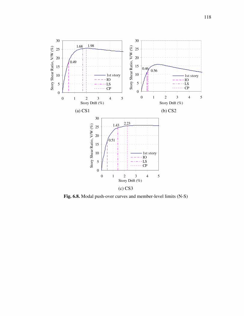
118

0.49

1.68 1.98

0

5

10

15

20

25

30

0 1 2 3 4 5Story Drift (%)

Sto

ry S

hea

r R

atio

, V/W

(%

) .

1st storyIOLSCP

0.460.56

0

5

10

15

20

25

30

0 1 2 3 4 5

Story Drift (%)

Sto

ry S

hea

r R

atio

, V/W

(%

) .

1st storyIOLSCP

(a) CS1 (b) CS2

0.51

1.43 2.23

0

5

10

15

20

25

30

0 1 2 3 4 5Story Drift (%)

Sto

ry S

hea

r R

atio

, V/W

(%

) .

1st storyIOLSCP

(c) CS3

Fig. 6.8. Modal push-over curves and member-level limits (N-S)

119

0.92

2.473.26

0

5

10

15

20

25

30

35

0 1 2 3 4 5 6 7Story Drift (%)

Sto

ry S

hea

r R

atio

, V/W

(%

)

.

2nd story

IO

LS

CP

0.89 1.07

0

5

10

15

20

25

30

35

0 1 2 3 4 5 6 7Story Drift (%)

Sto

ry S

hea

r R

atio

, V/W

(%

) .

1st storyIOLSCP

(a) CS1 (b) CS2

1.08

2.62 3.38

0

5

10

15

20

25

30

35

0 1 2 3 4 5 6 7Story Drift (%)

Sto

ry S

hea

r R

atio

, V/W

(%

) .

2nd story

IO

LS

CP

(c) CS3

Fig. 6.9. Critical response push-over curves and member-level limits (E-W)

120

1.01

2.48 3.20

0

5

10

15

20

25

30

35

40

0 1 2 3 4 5 6 7

Story Drift (%)

Sto

ry S

hea

r R

atio

, V/W

(%

) .

2nd storyIOLSCP

0.82 1.04

0

5

10

15

20

25

30

35

40

0 1 2 3 4 5 6 7

Story Drift (%)

Sto

ry S

hea

r R

atio

, V/W

(%

) .

1st storyIOLSCP

(a) CS1 (b) CS2

1.07

2.47 3.14

0

5

10

15

20

25

30

35

40

0 1 2 3 4 5 6 7Story Drift (%)

Sto

ry S

hea

r R

atio

, V/W

(%

) .

2nd storyIOLSCP

(c) CS3

Fig. 6.10. Critical response push-over curves and member-level limits (N-S)

121

y = 2.8292x0.8574

R2 = 0.8153

0

1

2

3

4

5

6

7

8

0.0 0.2 0.4 0.6 0.8 1.0

Sa (g)

Max

. In

ters

tory

Dri

ft (

%)

.y = 5.909x

0.8715

R2 = 0.7546

0

1

2

3

4

5

6

7

8

0.0 0.2 0.4 0.6 0.8 1.0

Sa (g)

Max

. In

ters

tory

Dri

ft (

%)

.

(a) CS1 (b) CS2

y = 3.4525x0.882

R2 = 0.856

0

1

2

3

4

5

6

7

8

0.0 0.2 0.4 0.6 0.8 1.0Sa (g)

Max

. In

ters

tory

Dri

ft (

%)

.

(c) CS3

Fig. 6.11. Development of member-level power law equations (E-W)

122

y = 3.4376x0.9342

R2 = 0.82

0

1

2

3

4

5

6

7

8

9

0.0 0.2 0.4 0.6 0.8 1.0Sa (g)

Max

. In

ters

tory

Dri

ft (

%)

y = 7.6037x1.0993

R2 = 0.8833

0

1

2

3

4

5

6

7

8

9

0.0 0.2 0.4 0.6 0.8 1.0Sa (g)

Max

. In

ters

tory

Dri

ft (

%)

(a) CS1 (b) CS2

y = 2.874x0.9079

R2 = 0.7656

0

1

2

3

4

5

6

7

8

9

0.0 0.2 0.4 0.6 0.8 1.0 1.2Sa (g)

Max

. In

ters

tory

Dri

ft (

%)

(c) CS3

Fig. 6.12. Development of member-level power law equations (N-S)

The uncertainty parameters in Eq. (6.1) are given in Table 6.8 for the global level

(GL), modal load pattern (MP) and critical response (CR) member-level fragility curves.

The uncertainty parameters associated with estimating the capacity and modeling the

structure ( CLβ and Mβ ) were estimated as 0.3 based on the values Wen et al. (2004) used

in developing fragility curves for RC frame members. The uncertainty associated with

the demand relationship, aD Sβ , was calculated for each set of data and ranged from

0.3787 to 0.5097.

123

Table 6.8. Uncertainty parameters for developing the fragility curves

E-W direction N-S direction Case study

Parameter

GL MP CR GL MP CR

s2 0.2048 0.2259 0.2096 0.1844 0.2421 0.1915

aD Sβ 0.4316 0.4573 0.4362 0.4114 0.4656 0.4186

CLβ 0.3 0.3 0.3 0.3 0.3 0.3 CS1

Mβ 0.3 0.3 0.3 0.3 0.3 0.3

s2 0.2319 0.2549 0.2549 0.1898 0.2164 0.2164

aD Sβ 0.4567 0.4765 0.4765 0.4169 0.4426 0.4426

CLβ 0.3 0.3 0.3 0.3 0.3 0.3 CS2

Mβ 0.3 0.3 0.3 0.3 0.3 0.3

s2 0.1542 0.1789 0.1561 0.2480 0.2967 0.2371

aD Sβ 0.3787 0.4056 0.3809 0.4707 0.5097 0.4613

CLβ 0.3 0.3 0.3 0.3 0.3 0.3 CS3

Mβ 0.3 0.3 0.3 0.3 0.3 0.3

The fragility curves for the member-level fragility analysis are shown in Figs.

6.13 and 6.14 for the modal push-over and in Figs. 6.15 and 6.16 for the critical response

push-over analysis. The member-level limits are considered to be more accurate than the

global limits, and the probabilities of exceedance are higher based on for the member-

level limits from the modal push-over analysis. The critical response fragility curves

more closely resemble the global level fragility curves, as the interstory drift limits based

on the critical response push-over analysis are closer to the global drift limits.

For most of the case studies, the LS and CP curves were closer together than the

IO fragility curves, especially for the critical response loading pattern. With the same

FEMA 356 rotation drift limits for CS2, the IO and LS fragility curves were identical.

For all fragility curve sets, the IMF CS2 has the largest fragility values.

124

0.0

0.2

0.4

0.6

0.8

1.0

0.0 0.2 0.4 0.6 0.8 1.0Sa (g)

P(L

S|S

a )

IO

LS

CP

(a) CS1

0.0

0.2

0.4

0.6

0.8

1.0

0.0 0.2 0.4 0.6 0.8 1.0Sa (g)

P(L

S|S

a )

IO

LS

CP

(b) CS2

0.0

0.2

0.4

0.6

0.8

1.0

0.0 0.2 0.4 0.6 0.8 1.0Sa (g)

P(L

S|S

a )

IO

LS

CP

(c) CS3

Fig. 6.13. Modal pattern member-level fragility curves (E-W)

125

0.0

0.2

0.4

0.6

0.8

1.0

0.0 0.2 0.4 0.6 0.8 1.0Sa (g)

P(L

S|S

a )

IO

LS

CP

(a) CS1

0.0

0.2

0.4

0.6

0.8

1.0

0.0 0.2 0.4 0.6 0.8 1.0Sa (g)

P(L

S|S

a )

IO

LS

CP

(b) CS2

0.0

0.2

0.4

0.6

0.8

1.0

0.0 0.2 0.4 0.6 0.8 1.0Sa (g)

P(L

S|S

a )

IO

LS

CP

(c) CS3

Fig. 6.14. Modal pattern member-level fragility curves (N-S)

126

0.0

0.2

0.4

0.6

0.8

1.0

0.0 0.2 0.4 0.6 0.8 1.0Sa (g)

P(L

S|S

a )

IO

LS

CP

(a) CS1

0.0

0.2

0.4

0.6

0.8

1.0

0.0 0.2 0.4 0.6 0.8 1.0Sa (g)

P(L

S|S

a )

IO

LS

CP

(b) CS2

0.0

0.2

0.4

0.6

0.8

1.0

0.0 0.2 0.4 0.6 0.8 1.0Sa (g)

P(L

S|S

a )

IO

LS

CP

(c) CS3

Fig. 6.15. Critical response member-level fragility curves (E-W)

127

0.0

0.2

0.4

0.6

0.8

1.0

0.0 0.2 0.4 0.6 0.8 1.0Sa (g)

P(L

S|S

a )

IO

LS

CP

(a) CS1

0.0

0.2

0.4

0.6

0.8

1.0

0.0 0.2 0.4 0.6 0.8 1.0Sa (g)

P(L

S|S

a )

IO

LS

CP

(b) CS2

0.0

0.2

0.4

0.6

0.8

1.0

0.0 0.2 0.4 0.6 0.8 1.0Sa (g)

P(L

S|S

a )

IO

LS

CP

(c) CS3

Fig. 6.16. Critical response member-level fragility curves (N-S)

128

6.2.3 Numerical Comparison

The probabilities of exceeding the LS and CP performance levels were compared

for the global level (GL), triangular push-over member-level (MP), and critical response

(CR) fragilities in Tables 6.9 through 6.12. For each case study, the probability of

exceeding the limit state for the median spectral acceleration (Sa) corresponding to each

building’s fundamental period for each of the Rix-Fernandez (RF) and Wen and Wu

(WW) sets of motions was computed.

Table 6.9. Probability of exceeding LS for 10% in 50 years Rix-Fernandez motions

P(LS|Sa) Modeling direction

Case study

Median Sa (g) GL MP CR

CS1 0.1295 0.05 0.07 0.02

CS2 0.1263 0.52 0.84 0.56 E-W

CS3 0.1378 0.09 0.23 0.03

CS1 0.1228 0.03 0.04 0.01

CS2 0.1188 0.37 0.81 0.42 N-S

CS3 0.1206 0.02 0.03 0.01

Table 6.10. Probability of exceeding LS 10% in 50 years Wen and Wu motions

P(LS|Sa) Modeling direction

Case study


CS1 0.0487 0.00 0.00 0.00

CS2 0.0406 0.06 0.29 0.08 E-W

CS3 0.0538 0.00 0.02 0.00

CS1 0.0393 0.00 0.00 0.00

CS2 0.0353 0.01 0.10 0.01 N-S

CS3 0.0375 0.00 0.00 0.00

129

Table 6.11. Probability of exceeding CP for 2% in 50 years Rix-Fernandez motions

P(CP|Sa) Modeling direction

Case study


CS1 0.6024 0.26 0.65 0.20

CS2 0.6141 0.88 1.00 0.98 E-W

CS3 0.5939 0.34 0.74 0.43

CS1 0.5942 0.17 0.65 0.25

CS2 0.6324 0.90 1.00 0.99 N-S

CS3 0.5791 0.12 0.41 0.23

Table 6.12. Probability of exceeding CP for 2% in 50 years Wen and Wu motions

P(CP|Sa) Modeling direction

Case study


CS1 0.4339 0.13 0.47 0.35

CS2 0.4148 0.73 0.99 0.97 E-W

CS3 0.4282 0.19 0.58 0.28

CS1 0.5652 0.15 0.63 0.28

CS2 0.4343 0.74 1.00 0.95 N-S

CS3 0.6360 0.14 0.36 0.20

The GL and CR probabilities were both lower than the MP probabilities as

dictated by the corresponding capacity limits. The RF motions generally produced

higher spectral accelerations for the building fundamental periods and corresponding

higher probabilities of exceedance than the WW motions, with the exception of CS3 in

the N-S direction. The probabilities of exceeding the performance levels were higher in

the E-W direction, determined to be the more vulnerable direction in the analysis and

evaluation discussed in Section 5.

The probabilities of exceeding the LS performance level for the 10% in 50 years

RF motions for CS2 were large, ranging from 52 to 84 percent for the qualitative

fragility analysis. Comparatively, the probabilities of exceeding the LS performance

level were between 2 and 7 percent for CS1 and 1 and 23 percent for CS3 for the RF

130

motions. The probabilities for exceeding the LS performance level for the 10% in 50

years WW motions were much lower.

For the 2% in 50 years RF motions, the probabilities of exceeding the CP

performance level were between 88 and 100 percent for CS2. These values were lower

for CS1 and CS3 for exceeding the CP performance level (26 to 65 percent probability

and a 34 to 74 percent probability, respectively). These ranges were similar for the WW

motions.

6.3 Quantitative Limits

In addition to the FEMA 356 drift limits, quantitative interstory drift limits based

on the member behavior were also used to define the drift capacity. The two limits used

in this study were suggested by Wen et al. (2004):

1) First Yield (FY) – Interstory drift at which a member first begins to yield

under applied lateral loading

2) Plastic Mechanism Initiation (PMI) – Interstory drift at which a story

mechanism or an overall beam sidesway mechanism initiates under applied

lateral loading

The interstory drift limits at which FY and PMI initiate are given in Table 6.13

and Figs. 6.17 and 6.18 for each case study. These drift limits were determined using the

inverted triangular load pattern from the member-level fragility analysis. This pattern for

the first story was determined to provide the critical drifts from the member-level

analysis. Yielding for FY was determined when the moment curvature of the section

reached a yield plateau. PMI was reached when all the columns or beams in story

yielded at the member ends. These terms are discussed in more detail in Section 2.

131

Table 6.13. Quantitative interstory drift limits

Drift limit (%)

E-W direction N-S direction

Case study

FY PMI FY PMI

CS1 0.36 1.55 0.36 1.18

CS2 0.53 1.98 0.41 1.41

CS3 0.55 1.51 0.38 1.32

0.36

1.55

0

1

2

3

4

5

6

7

8

9

0 1 2 3 4 5Story Drift (%)

Sto

ry S

hea

r, V

/W (

%)

1st storyFYPMI

0.53

1.98

0

1

2

3

4

5

6

7

8

9

0 1 2 3 4 5Story Drift (%)

Sto

ry S

hea

r, V

/W (

%)

1st storyFYPMI

(a) CS1 (b) CS2

0.55

1.51

0

1

2

3

4

5

6

7

8

9

0 1 2 3 4 5Story Drift (%)

Sto

ry S

hea

r, V

/W (

%)

1st storyFYPMI

(c) CS3

Fig. 6.17. Triangular push-over curves and quantitative limits (E-W)

132

0.36

1.18

0

2

4

6

8

10

12

14

16

0 1 2 3 4 5Story Drift (%)

Sto

ry S

hea

r, V

/W (

%)

1st storyFYPMI

0.38

1.32

0

2

4

6

8

10

12

14

16

0 1 2 3 4 5Story Drift (%)

Sto

ry S

hea

r, V

/W (

%)

1st storyFYPMI

(a) CS1 (b) CS2

0.41

1.41

0

2

4

6

8

10

12

14

16

0 1 2 3 4 5Story Drift (%)

Sto

ry S

hea

r, V

/W (

%)

1st storyFYPMI

(c) CS3

Fig. 6.18. Triangular push-over curves and quantitative limits (N-S)

Fig. 6.19 shows the locations of inelastic rotation at the PMI performance level in

the E-W direction. For CS2 and CS3, the exterior frame did not fully yield before the

ultimate capacities of the wide-module joists in the interior frames were reached. For

these two cases, the PMI limit state was recorded at the drift where each of the interior

wide-module joists exceeded their capacities. The inelastic rotation locations

corresponding to PMI for CS2 and CS3 are very similar.

The locations of inelastic rotation at the PMI limit state for the N-S model are

shown in Fig. 6.20. The effects of the different beam-column strength ratios can be

observed in the initiation of the plastic mechanism. For CS2, with a column-to-beam

133

strength ratio of 0.8, almost all the story hinging occurred at the columns. CS1 and CS3

had column-to-beam strength ratios greater than 1.4, and the beams yielded before the

columns in many of the bays.

Exterior (typ.) Interior (typ.)

(a) CS1

(b) CS2

(c) CS3

Fig. 6.19. Locations of inelastic rotation at PMI for triangular push-over (E-W)

= Plastic hinge

134

Exterior (typ.) Interior (typ.) Interior (typ.)

(a) CS1

(b) CS2

(c) CS3

Fig. 6.20. Locations of inelastic rotation at PMI for triangular push-over (N-S)

The fragility curves corresponding to the quantitative FY and PMI limit states are

shown in Figs. 6.21 and 6.22. As in the qualitative analysis, CS2 had the highest

probability of exceeding both limit states for both model directions. For the E-W

direction, CS3 showed the lowest probability of exceeding the FY limit state, while CS1

showed the lowest probability of exceeding the PMI limit state. For the N-S direction,

CS1 showed the lowest probabilities of exceeding both FY and PMI.

= Plastic hinge

135

0.0

0.2

0.4

0.6

0.8

1.0

0.0 0.2 0.4 0.6 0.8 1.0Sa (g)

P(L

S|S

a )

FY

PMI

(a) CS1

0.0

0.2

0.4

0.6

0.8

1.0

0.0 0.2 0.4 0.6 0.8 1.0Sa (g)

P(L

S|S

a )

FY

PMI

(b) CS2

0.0

0.2

0.4

0.6

0.8

1.0

0.0 0.2 0.4 0.6 0.8 1.0Sa (g)

P(L

S|S

a )

FY

PMI

(c) CS3

Fig. 6.21. Quantitative fragility curves (E-W)

136

0.0

0.2

0.4

0.6

0.8

1.0

0.0 0.2 0.4 0.6 0.8 1.0Sa (g)

P(L

S|S

a )

FY

PMI

(a) CS1

0.0

0.2

0.4

0.6

0.8

1.0

0.0 0.2 0.4 0.6 0.8 1.0Sa (g)

P(L

S|S

a )

FY

PMI

(b) CS2

0.0

0.2

0.4

0.6

0.8

1.0

0.0 0.2 0.4 0.6 0.8 1.0Sa (g)

P(L

S|S

a )

FY

PMI

(c) CS3

Fig. 6.22. Quantitative fragility curves (N-S)

137

6.4 Selection of Default Fragility Curves

6.4.1 General

A default set of fragility curves was determined from the four sets of fragility

curves developed from the FEMA 356 and quantitative limits for implementation into

loss estimation software, such as MAEviz developed by the MAE Center (2006). Three

performance levels were selected from the FEMA 356 and quantitative fragility curves,

defined generically as Performance Level 1 (PL1), PL2, and PL3. Based on work by Bai

et al. (2007), damage states are defined based on these performance levels, as shown in

Fig. 6.23. The four damage states are classified as insignificant (I), moderate (M), heavy

(H), and complete (C) damage.

Fig. 6.23. Relationship between performance levels and damage states (Bai et al. 2007)

6.4.2 Default Fragility Curves

To define the generic performance levels for the default fragility curves for each

case study, a combination of the member-level FEMA 356 performance levels and the

quantitative limit states were used. The FEMA 356 member-level performance levels

(IO, LS, and CP) using the modal push-over pattern (MP) were more specific to the

138

structural detailing and geometry than the global-level performance limits and more

conservative than the critical response (CR) limits. However, for CS2 the IO and LS

limits were the same for the MP limits; therefore, the CR limits were used for PL2. The

quantitative limit state, PMI, was used as the third performance level in all of the case

studies except of CS1 and CS3 in the N-S direction. The generic performance levels for

each case study and direction are given in Table 6.14 along with the corresponding

interstory drift limits.

Table 6.14. Performance levels and corresponding interstory drift (%) limits for default fragility curves

Direction Case study PL1 PL2 PL3

CS1 IO(MP) = 0.46 LS(MP) = 1.20 PMI = 1.55

CS2 IO(MP) = 0.52 LS(CR) = 0.89 PMI = 1.98 E-W

CS3 IO(MP) = 0.49 LS(MP) = 0.93 PMI = 1.51

CS1 IO(MP) = 0.49 LS(MP) = 1.68 CP(MP) = 1.98

CS2 IO(MP) = 0.46 LS(CR) = 0.82 PMI = 1.41 N-S

CS3 IO(MP) = 0.45 LS(MP) = 1.42 CP(MP) = 2.23

The generic performance levels are shown along with the remaining limit states

for each case study in Figs. 6.24 through 6.35. The emphasized fragility curves in the

first of two figures for each case study and direction correspond to those listed in Table

6.14, and the second figure shows the final performance levels with the corresponding

damage states.

139

0.0

0.2

0.4

0.6

0.8

1.0

0.0 0.2 0.4 0.6 0.8 1.0

Sa (g)

P(L

S|S

a )

.

ML IO

ML LS

ML CP

CR IO

CR LS

CR CP

GL IO

GL LS

GL CP

FY

PMI

Fig. 6.24. Selection of default fragility curves for CS2 (E-W)

0.0

0.2

0.4

0.6

0.8

1.0

0.0 0.2 0.4 0.6 0.8 1.0

Sa (g)

P(L

S|S

a )

.

PL1

PL2

PL3

I

M

H

C

Fig. 6.25. Default fragility curves for CS1 (E-W)

140

0.0

0.2

0.4

0.6

0.8

1.0

0.0 0.2 0.4 0.6 0.8 1.0

Sa (g)

P(L

S|S

a )

.

ML IO

ML LS

ML CP

CR IO

CR LS

CR CP

GL IO

GL LS

GL CP

FY

PMI


0.0

0.2

0.4

0.6

0.8

1.0

0.0 0.2 0.4 0.6 0.8 1.0

Sa (g)

P(L

S|S

a )

.

PL1

PL2

PL3

I

M

H

C


141

0.0

0.2

0.4

0.6

0.8

1.0

0.0 0.2 0.4 0.6 0.8 1.0Sa (g)

P(L

S|S

a )

.

ML IO

ML LS

ML CP

CR IO

CR LS

CR CP

GL IO

GL LS

GL CP

FY

PMI


0.0

0.2

0.4

0.6

0.8

1.0

0.0 0.2 0.4 0.6 0.8 1.0

Sa (g)

P(L

S|S

a )

.

PL1

PL2

PL3

I

M

H

C


142

0.0

0.2

0.4

0.6

0.8

1.0

0.0 0.2 0.4 0.6 0.8 1.0

Sa (g)

P(L

S|S

a )

.

ML IO

ML LS

ML CP

GL IO

GL LS

GL CP

CR IO

CR LS

CR CP

FY

PMI

Fig. 6.30. Selection of default fragility curves for CS1 (N-S)

0.0

0.2

0.4

0.6

0.8

1.0

0.0 0.2 0.4 0.6 0.8 1.0

Sa (g)

P(L

S|S

a )

.

PL1

PL2

PL3

I

M

H

C

Fig. 6.31. Default fragility curves for CS1 (N-S)

143

0.0

0.2

0.4

0.6

0.8

1.0

0.0 0.2 0.4 0.6 0.8 1.0

Sa (g)

P(L

S|S

a )

.

ML IO

ML LS

ML CP

GL IO

GL LS

GL CP

CR IO

CR LS

CR CP

FY

PMI


0.0

0.2

0.4

0.6

0.8

1.0

0.0 0.2 0.4 0.6 0.8 1.0

Sa (g)

P(L

S|S

a )

.

PL1

PL2

PL3

IM

H

C


144

0.0

0.2

0.4

0.6

0.8

1.0

0.0 0.2 0.4 0.6 0.8 1.0

Sa (g)

P(L

S|S

a )

.

ML IO

ML LS

ML CP

GL IO

GL LS

CL CP

CR IO

CR LS

CR CP

FY

PMI


0.0

0.2

0.4

0.6

0.8

1.0

0.0 0.2 0.4 0.6 0.8 1.0

Sa (g)

P(L

S|S

a )

.

PL1

PL2

PL3

I

M

H

C


145

6.4.3 MAEviz Implementation

MAEviz (MAE Center 2006) is a seismic risk assessment software, developed

through a joint effort between the Mid-America Earthquake (MAE) Center and the

National Center for Supercomputing Application (NCSA). The program uses enhanced

graphics and user input options within the consequence-based risk management

methodology to generate damage estimates based on extensive research and

development of earthquake hazards and seismic performance. The goal of the program is

to assist policy-makers and decision-makers in developing risk reduction strategies and

implementing mitigation actions.

To simplify the fragility equations and reduce the number of parameters, Eq.

(6.2) is used to implement the fragility relationships into MAEviz.

ln( | ) a C

a

C

SP LS S

λ

β

−= Φ

(6.2)

where:

P(LS | Sa) = Probability of exceeding a limit state given a spectral acceleration value

Φ = Standard normal cumulative distribution function Sa = Spectral acceleration (g) λC¸ βC = Modification parameters

The original parameters used to describe the fragility curves [Eq. (6.1)] are

different than those in used in the MAEviz simplified equation in Eq. (6.2). As a result,

new fragility curves were fitted to the original fragility curve relationships to determine

the parameters for the MAEviz fragility expressions, as shown in Fig. 6.36 for CS1 in

the E-W direction. The parameters for the MAEviz expressions for each case study are

given in Table 6.15.

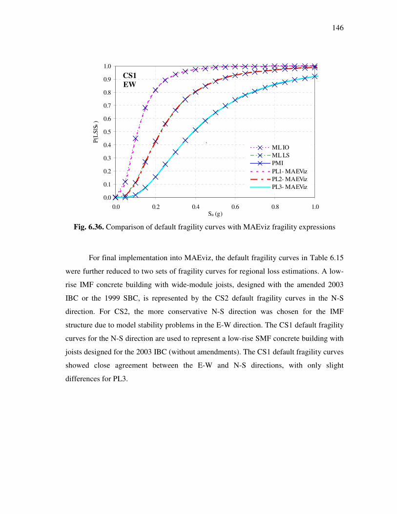
146

0.0

0.1

0.2

0.3

0.4

0.5

0.6

0.7

0.8

0.9

1.0

0.0 0.2 0.4 0.6 0.8 1.0Sa (g)

P(L

S|S

a )

.

ML IO

ML LS

PMI

PL1- MAEViz

PL2- MAEViz

PL3- MAEViz

`

Fig. 6.36. Comparison of default fragility curves with MAEviz fragility expressions

For final implementation into MAEviz, the default fragility curves in Table 6.15

were further reduced to two sets of fragility curves for regional loss estimations. A low-

rise IMF concrete building with wide-module joists, designed with the amended 2003

IBC or the 1999 SBC, is represented by the CS2 default fragility curves in the N-S

direction. For CS2, the more conservative N-S direction was chosen for the IMF

structure due to model stability problems in the E-W direction. The CS1 default fragility

curves for the N-S direction are used to represent a low-rise SMF concrete building with

joists designed for the 2003 IBC (without amendments). The CS1 default fragility curves

showed close agreement between the E-W and N-S directions, with only slight

differences for PL3.

CS1 EW

147

Table 6.15. Fragility curve parameters for MAEviz

Direction Case study Limit state λC βC

PL1 -2.11

PL2 -1.00 N-S

PL3 -0.69

0.72

PL1 -2.00

PL2 -0.93

CS1

E-W

PL3 -0.78

0.68

PL1 -2.63

PL2 -0.93 N-S

PL3 -0.78

0.58

PL1 -2.70

PL2 -2.16

CS2

E-W

PL3 -1.23

0.725

PL1 -1.89

PL2 -0.78 N-S

PL3 -0.28

0.73

PL1 -2.20

PL2 -1.48

CS3

E-W

PL3 -0.94

0.66

148

7 SUMMARY, CONCLUSIONS AND RECOMMENDATIONS

7.1 Summary

The objective of this study was to evaluate the seismic performance of a four-

story reinforced concrete (RC) moment frame designed according to the provisions of

three building codes of significance in the Central United States. Case Study 1 (CS1)

was designed with the 2003 International Building Code (IBC) (ICC 2003) and had a

design base shear of 7.2% W, while CS2 designed with the 2003 IBC with local

amended seismic provisions (City of Memphis and Shelby County 2005) had a design

base shear of 3.8% W. The design base shear for CS3 was 4.2% W using the 1999

Standard Building Code (SBC) (SBCCI).

Higher design accelerations classified CS1 and CS3 as Seismic Design Category

(SDC) D, requiring a special moment frame (SMF) lateral system. CS2 was classified as

SDC C, permitting the use of an intermediate moment frame (IMF). It should be noted

that the SBC design was just above the cut-off for SDC D and could qualify as SDC C

for slightly different conditions. The lateral system type had the largest influence on the

seismic performance of the case study structures. Another critical factor was the number

of moment frames required in each direction. In the long (E-W) direction, higher drift

demands and redundancy provisions required moment frames along each column line for

CS1, while CS2 and CS3 were only required to have exterior lateral frames.

Static push-over and dynamic analyses with synthetic ground motions developed

for 2% and 10% probabilities of exceedance in 50 years for Memphis, Tennessee, were

used in the performance evaluation. The performance difference between lateral systems

is most evident in the N-S (short) direction, for which the same number of moment

frames is used for each case study. The N-S push-over analysis showed that the SMF

buildings had approximately 1.5 times the strength capacity and ductility of the IMF

building. Furthermore, for the 2% in 50 years ground motions, the CS2 model became

149

unstable when the capacities of the wide-module joists were exceeded in the more

vulnerable E-W direction, and a first story mechanism formed in the N-S model.

In the FEMA 356 global interstory drift evaluation, each case study met LS

performance for the 10% in 50 years motions. CS1 and CS3 satisfied CP performance

for the 2% in 50 years motions, but first story drifts in CS2 resulting from the story

mechanism exceeded the CP performance level for the 2% in 50 years hazard. For the

more detailed member-level evaluation based on plastic rotation limits, CS2 was the

only case study that did not meet LS performance for the 10% in 50 years motions. None

of the case studies satisfied the CP performance level for the 2% in 50 years event. The

median maximum column plastic rotations of the SMF case studies for the 2% in 50

years event were a maximum of two times the CP rotation limits in a few locations, as

compared to as much as 18 times the CP limits for the CS2 columns. The exceedance of

the plastic rotation limits by the SMFs may indicate that the FEMA 356 limits for RC

frame members are quite conservative. However, it is recognized that the 2% in 50 years

Memphis motions have significant spectral acceleration values.

The Basic Safety Objective (BSO) in FEMA 356 reflects the general seismic

design code philosophy to accomplish two limited performance objectives: (1) to resist

higher probability of occurrence earthquakes (10% probability of exceedance in 50

years) without loss of life (Life Safety or LS); and (2) to withstand lower probability

earthquakes (2% probability of exceedance in 50 years) without collapse (Collapse

Prevention or CP). CS1 and CS3 met the BSO for the global drift evaluation, but the

second performance objective was not met for the more detailed member-level

evaluation. CS2 did not meet either of the BSO performance objectives.

7.2 Conclusions

This study shows the expected demands and resulting damage for a Central U.S.

RC frame building designed according to the building codes currently adopted in

Memphis, Tennessee. These building codes are also applicable in other parts of the

Central U.S., and the structure type considered is relatively common. The following

conclusions were drawn for this study:

150

1. The comparative performance evaluation of the three case study designs

underscores the importance of the lateral system type (seismic detailing) in the

seismic performance. Even with relatively different design base shears, the IBC

and SBC designs with special moment frames (SMFs) met the same FEMA 356

performance objectives. In contrast, the intermediate moment frame (IMF)

designed with the IBC with local seismic amendments exhibited lower

performance and did not meet either Life Safety (LS) for 10% in 50 years or

Collapse Prevention (CP) performance for 2% in 50 years for the member-level

evaluation. Differences in the structural performance of each lateral resisting

system were also evident in the nonlinear analysis responses and the fragility

curves.

2. Redundancy provisions and higher drift demands also impacted the performance

of the case studies, but to a lesser extent than the lateral system type. The 2003

IBC was the only building code that included redundancy provisions for the

redistribution of lateral forces, which can restrict the moment frame layout. The

higher design drift demands associated with the higher design base shears

influenced the column sizes.

3. The maximum interstory drifts for each case study for the 10% probability of

exceedance in 50 years event were similar and within suggested LS global

interstory drift values. However, the fragility curves show that there is still a

considerable probability of exceeding the LS performance level for the amended

IBC designed building for the 10% in 50 years ground motion based on the

member-level evaluation. Conversely, the probabilities of exceeding the LS

performance level for the SMF case studies were very low for the same hazard

level.

4. For the 2% in 50 years hazard, the case study structure designed with the 2003

IBC with local Memphis seismic amendments (CS2) has a significant probability

of exceeding the CP performance level. The CS2 building model became

unstable when the wide-module joist capacities were exceeded in the more

151

vulnerable long (E-W) direction under the 2% in 50 years motions, and a story

mechanism formed in the short (N-S) direction with predicted first story drifts of

greater than 7%.

5. For the 2% in 50 years Memphis motions, the case study buildings designed as

SMFs showed substantially better performance than the IMF building based on

the nonlinear analysis and FEMA 356 performance evaluation.

6. FEMA 356 member-level CP plastic rotation limits for RC frames were exceeded

by the case studies designed for the most up-to-date seismic code (IBC 2003) for

the 2% in 50 years motions, which may indicate that these limits are conservative.

7. The differences in the fragility curves for the special and intermediate moment

frame buildings show the importance of knowing the type of lateral system when

selecting fragility curves to predict the probabilities of exceeding limits states for

a given earthquake intensity.

7.3 Recommendations for Future Research

The work in this study was limited to a four-story concrete moment frame

building with a wide-module joist floor system. The case study performance was

dependent on the structural layout; therefore, the performance would vary for different

types of structural configurations such as irregular structures and structures with a

greater or lesser number of stories. Some recommendations for complementary research

are listed below.

1. Investigating different structural types and configurations using the same

methodology would broaden the scope of determining the impact of current

building code seismic provisions in the Central U.S. Additional structural types

might include special and intermediate steel moment frames, taller RC frames,

or RC shear wall systems.

2. The building site for this study was located in downtown Memphis, which has

some of the largest seismic design values in the Memphis area. As mentioned

previously, slightly lower seismic design values in the 1999 SBC design would

152

classify the case study structure as Seismic Design Category C, requiring less

seismic detailing, and would significantly affect the performance. Running a

similar analysis with an intermediate moment frame for the 1999 SBC design

instead of a special moment frame to determine the effect on the performance

might be useful.

3. This study utilized synthetic ground motions developed for the Memphis area.

To apply this study to a larger region, ground motions for other vulnerable areas

in the New Madrid Seismic Zone could also be investigated.

4. A more in-depth cost assessment for the special and intermediate moment frame

buildings would be useful in determining practical cost-benefit ratios of

designing for improved seismic performance.

153

REFERENCES

Abrams, D. P., and Shinozuka, M., ed. (1997). "Loss assessment of Memphis buildings." Technical Report NCEER-97-0018. National Center for Earthquake Engineering Research, Buffalo, NY.

ACI Committee 318. (1995). Building Code Requirements for Reinforced Concrete (ACI

318-95), American Concrete Institute, Detroit, MI.

ACI Committee 318. (2002). Building Code Requirements for Reinforced Concrete (ACI

318-02), American Concrete Institute, Farmington, MI.

AISC. (2005). Steel Construction Manual, American Institute of Steel Construction, Inc., Chicago, IL.

ASCE. (1995). ASCE Minimum Design Loads for Buildings and Other Structures (ASCE

7-95), American Society of Civil Engineers, Washington, DC.

ASCE. (2000). Prestandard and Commentary for the Seismic Rehabilitation of Buildings

(FEMA 356), American Society of Civil Engineers, Washington, DC.

ASCE. (2002). ASCE Minimum Design Loads for Buildings and Other Structures (ASCE

7-02), American Society of Civil Engineers, Washington, DC.

Bai, J. W., Hueste, M. B., and Gardoni, P. (2007) "Assessment of the expected seismic structural losses for buildings in Mid-America." submitted to Journal of

Structural Engineering.

Beavers, J. (2002). "A review of seismic hazard description in US design codes and procedures." Progress of Structural Engineering Materials, 4, 46-63.

BSSC. (1992). NEHRP Recommended Provisions for the Development of Seismic

Regulations for New Buildings, Part 1: (Provisions) and Part II: (Commentary), Building Seismic Safety Council, Washington, DC.

BSSC. (1998). NEHRP Recommended Provisions for Seismic Regulations for New

Buildings and Other Structures, Part 1: (Provisions) and Part II: (Commentary), Building Seismic Safety Council, Washington, DC.

BSSC. (2004). NEHRP Recommended Provisions for Seismic Regulations of New

Buildings and Other Structures Part 1: Provisions (FEMA 450), Building Seismic Safety Council, Washington, DC.

154

City of Memphis and Shelby County. (2005). "Appendix L- Alternate Seismic Protection Calculations and Procedures." Memphis and Shelby County 2005 Joint Building Code Local Amendments, Memphis, TN.

Cornell, C. A., Jalayer, F., Hamburger, R. O., and Foutch, D. A. (2002). "Probabilistic basis for the 2000 SAC Federal Emergency Management Agency steel moment frame guidelines." Journal of Structural Engineering, 128(4), 526-533.

CSI. (2002). An Introduction to ETABS: Version 8, Computers and Structures, Inc., Berkeley, CA.

CUSEC. (2007). "New Madrid Seismic Zone." Central United States Earthquake Consortium, <http://www.cusec.org/S_zones/NMSZ/nmsz_home.htm> (Nov. 12, 2007).

Dooley, K. L., and Bracci J. M. (2001). "Seismic evaluation of column-to-beam strength ratios in reinforced concrete frames." ACI Structural Journal, 98(6), 843-851.

Dowty, S., and Ghosh, S. K. (2002). "IBC structural provisions: A better alternative." Building Standards, 12-16.

Elnashai, A. S., Papanikolaou, V. and Lee, D.H. (2002). ZEUS-NL User Manual, Mid-America Earthquake Center, University of Illinois at Urbana-Champaign.

Erberik, M. A., and Elnashai, A.S. (2004). "Fragility analysis of flat-slab structures." Engineering Structures, 26, 937–948.

FEMA. (1985). "An Assessment of Damage and Casualties for Six Cities in the Central United States Resulting from Earthquakes in the New Madrid Seismic Zones." Prepared under contract EMK-C-0057 (CUSEPP), Federal Emergency Management Agency, Washington, DC.

Fernández, J., and Rix, G. (2006). "Soil attenuation relationships and seismic hazard analyses in the Upper Mississippi Embayment." Eighth U.S. National Conference on Earthquake Engineering 8NCEE, San Francisco, CA.

Francis, S., and Stone, J. (1998). "The International Building Code and its impact on wood-frame design and construction." 1998 ASAE Annual International Meeting, Orlando, FL.

French, S., and Muthukumar, S. (2004). "Shelby County Inventory Database." Mid-America Earthquake Center, University of Illinois at Urbana-Champaign.

Hamburger, R., and Kircher, C. (2000). "Recent developments in seismic design: Methodologies and codes." Earthquake Spectra, 16(1), vii-xiii.

155

Hayes, J. R., Woodson, S. C., Pekelnicky, R. G., Poland, C. D., Corely, W. G., and Sozen, M. (2005). "Can strengthening for earthquake improve blast and progressive collapse resistance?" Journal of Structural Engineering, 131(8), 1157-1177.

Holmes, W. (2000). "The 1997 NEHRP recommended provisions for seismic regulations for new buildings and other structures." Earthquake Spectra, 16(1), 101-114.

Hueste, M. B., and Bai, J. W. (2007). "Seismic retrofit of a reinforced concrete flat-slab structure: Part I- seismic performance evaluation." Engineering Structures, 29(6), 1165-1177.

Hwang, H. H. M., and Huo, J-R. (1997). "A method for earthquake motion-damage relationships with application to reinforced concrete frames." Loss-Assessment of Memphis buildings. Technical Report NCEER 97-0008, National Center for Earthquake Engineering Research, Buffalo, NY.

ICC. (2003). International Building Code (IBC 2003), International Code Council, Falls Church, VA.

Jeong, S. H., and Elnashai, A. S. (2005). "Analytical assessment of an irregular RC frame for full scale 3D pseudo-dynamic testing Part I: Analytical model verification." Journal of Earthquake Engineering 9(1), 95-128.

Kalkan, E., and Kunnath, S. (2006). "Assessment of current nonlinear static procedures for seismic evaluation of buildings." Engineering Structures, 29, 305-316.

Karayannis, C. G., Izzuddin, B. A. and Elnashai, A. S. (1994). "Application of adaptive analysis to reinforced concrete frames." Journal of Structural Engineering, 120(10), 2935-2957.

Kinali, K., and Ellingwood, B.R. (2007). "Seismic fragility assessment of steel frames for consequence-based engineering: A case study for Memphis, TN." Engineering Structures, 29(6), 1115-1127.

Krawinkler, H., and Seneviratna, G. D. P. K. (1998). "Pros and cons of a pushover analysis of seismic performance evaluation." Engineering Structures, 20(4-6), 452-464.

Leyendecker, E. V., Hunt, R. J., Frankel, A. D., and Rukstales, K. S. (2000). "Development of maximum considered earthquake ground motion maps." Earthquake Spectra, 16(1), 21-40.

Mander, J. B., Priestley, J.N., and Park, R. (1988). "Observed stress-strain behavior of confined concrete." Journal of Structural Engineering, 114(8), 1827-1849.

156

Mid-America Earthquake Center. (2006). "Earthquake Risk Assessment Using MAEviz." University of Illinois at Urbana-Champaign.

Mwafy, A. M., and Elnashai, A. S. (2001). "Static pushover versus dynamic collapse analysis of RC buildings." Engineering Structures, 23(5), 407-424.

Pezeshk, S. (2004). "Site specific considerations in seismic design." West Tennessee Structural Engineer's Association, Memphis, Tennessee. <http://www.ce. memphis.edu/WTNSEA/Site%20Specific%20Considerations%20in%20Seismic-for%20web%20page.pdf> (Oct. 2, 2006).

Ramamoorthy, S., Gardoni, P., and Bracci, J. (2006). "Probabilistic demand models and fragility curves for reinforced concrete frame." Journal of Structural Engineering, 132(10), 1563-1572.

Rix, G. J., and Fernandez, J.A. (2006). "Probabilistic ground motions for selected cities in the Upper Mississippi Embayment." Georgia Tech, <http://www.ce.gatech.edu /~geosys/soil_dynamics/research/groundmotionsembay/> (Apr. 6, 2006).

Romero, S., and Rix, G. (2001). "Regional variation in near surface shear wave velocity in the Greater Memphis area." Engineering Geology, 62, 137-158.

RS Means. (2007). Building Construction Cost Data 65th Annual Edition, R.S. Means Construction Publishers & Consultants, Kingston, MA.

Sadjadi, R., Kianoush, M.R., and Talebi, S. (2007). "Seismic performance of reinforced concrete moment resisting frames." Engineering Structures, in press.

SBCCI. (1999). Standard Building Code (SBC), Southern Building Code Congress International, Birmingham, AL.

Singhal, A., and Kiremidjian, A. S. (1997). "A method for earthquake motion-damage relationships with application to reinforced concrete frames." Technical Report

NCEER 97-0008. National Center for Earthquake Engineering Research, Buffalo, NY.

Street, R. L., and Nuttli, O. W. (1990). "The great central Mississippi valley earthquakes of 1811-1812." University of Kentucky, Lexington.

Trifunac, M. D., and Brady, A.G. (1975). "A study on the duration of strong earthquake ground motion." Bulletin of the Seismological Society of America, 65(3), 581-626.

Wen, T. K., and Wu, C. L. (2000). "Generation of ground motions for Mid-America cities." Mid-America Earthquake (MAE) Center <http:/mae.ce.uiuc.edu/newsite/ research/rr-1/gmotions/index.html> (27 Jan. 2000).

157

Wen, T. K., Ellingwood, B. R., and Bracci, J. M. (2004). "Vulnerability functions." Mid-America Earthquake Center, University of Illinois at Urbana-Champaign.

Wen, Y. K., Ellingwood, B.R., Veneziano, D. and Bracci, J.M. (2003). "Uncertainity Modeling in Earthquake Engineering." Mid-America Earthquake (MAE) Center Project FD-2 Report, Urbana, IL.

158

APPENDIX A GROUND MOTION TIME HISTORIES

The acceleration time histories for both the Rix and Fernandez ground motion

records (see Section 4.3) and the Wen and Wu ground motions records (see Section

6.1.2) are provided. The vertical dotted line denotes the time step at which 95 percent of

the earthquake energy is imparted, discussed in Section 4.3.

-0.4

-0.2

0.0

0.2

0.4

0 20 40 60 80Time (s)

Acc

eler

atio

n (g)

.

-0.4

-0.2

0.0

0.2

0.4

0 20 40 60 80Time (s)

Acc

eler

atio

n (g)

.

(a) 2475_01wu (b) 2475_02wu

-0.4

-0.2

0.0

0.2

0.4

0 20 40 60 80Time (s)

Acc

eler

atio

n (g)

.

-0.4

-0.2

0.0

0.2

0.4

0 20 40 60 80Time (s)

Acc

eler

atio

n (g)

.

(c) 2475_03wu (d) 2475_04wu

Fig. A.1. Acceleration time histories for 2% in 50 years Wen and Wu motions

159

-0.4

-0.2

0.0

0.2

0.4

0 20 40 60 80Time (s)

Acc

eler

atio

n (g)

.

-0.4

-0.2

0.0

0.2

0.4

0 20 40 60 80Time (s)

Acc

eler

atio

n (g)

.

(e) 2475_05wu (f) 2475_06wu

-0.4

-0.2

0.0

0.2

0.4

0 20 40 60 80Time (s)

Acc

eler

atio

n (g)

.

-0.4

-0.2

0.0

0.2

0.4

0 20 40 60 80Time (s)

Acc

eler

atio

n (g)

.

(g) 2475_07wu (h) 2475_08wu

-0.4

-0.2

0.0

0.2

0.4

0 20 40 60 80Time (s)

Acc

eler

atio

n (g)

.

-0.4

-0.2

0.0

0.2

0.4

0 20 40 60 80Time (s)

Acc

eler

atio

n (g)

.

(i) 2475_09wu (j) 2475_010wu

Fig. A.1. Continued.

160

-0.4

-0.2

0.0

0.2

0.4

0 20 40 60 80Time (s)

Acc

eler

atio

n (g)

.

-0.4

-0.2

0.0

0.2

0.4

0 20 40 60 80Time (s)

Acc

eler

atio

n (g)

.

(a) 475_01wu (b) 475_02wu

-0.4

-0.2

0.0

0.2

0.4

0 20 40 60 80Time (s)

Acc

eler

atio

n (g)

.

-0.4

-0.2

0.0

0.2

0.4

0 20 40 60 80Time (s)

Acc

eler

atio

n (g)

.

(c) 475_03wu (d) 475_04wu

-0.4

-0.2

0.0

0.2

0.4

0 20 40 60 80Time (s)

Acc

eler

atio

n (g)

.

-0.4

-0.2

0.0

0.2

0.4

0 20 40 60 80Time (s)

Acc

eler

atio

n (g)

.

(e) 475_05wu (f) 475_06wu

Fig. A.2. Acceleration time histories for 10% in 50 years Wen and Wu motions

161

-0.4

-0.2

0.0

0.2

0.4

0 20 40 60 80Time (s)

Acc

eler

atio

n (g)

.

-0.4

-0.2

0.0

0.2

0.4

0 20 40 60 80Time (s)

Acc

eler

atio

n (g)

.

(g) 475_07wu (h) 475_08wu

-0.4

-0.2

0.0

0.2

0.4

0 20 40 60 80Time (s)

Acc

eler

atio

n (g)

.

-0.4

-0.2

0.0

0.2

0.4

0 20 40 60 80Time (s)

Acc

eler

atio

n (g)

.

(i) 475_09wu (j) 475_010wu


162

-0.4

-0.2

0.0

0.2

0.4

0 20 40 60 80Time (s)

Acc

eler

atio

n (g)

.

-0.4

-0.2

0.0

0.2

0.4

0 20 40 60 80Time (s)

Acc

eler

atio

n (g)

.

(a) 2475_01 (b) 2475_02

-0.4

-0.2

0.0

0.2

0.4

0 20 40 60 80Time (s)

Acc

eler

atio

n (g)

.

-0.4

-0.2

0.0

0.2

0.4

0 20 40 60 80Time (s)

Acc

eler

atio

n (g)

.

(c) 2475_03 (d) 2475_04

-0.4

-0.2

0.0

0.2

0.4

0 20 40 60 80Time (s)

Acc

eler

atio

n (g)

.

-0.4

-0.2

0.0

0.2

0.4

0 20 40 60 80Time (s)

Acc

eler

atio

n (g)

.

(e) 2475_05 (f) 2475_06

Fig. A.3. Acceleration time histories for 2% in 50 years Rix and Fernandez motions

163

-0.4

-0.2

0.0

0.2

0.4

0 20 40 60 80Time (s)

Acc

eler

atio

n (g)

.

-0.4

-0.2

0.0

0.2

0.4

0 20 40 60 80Time (s)

Acc

eler

atio

n (g)

.

(g) 2475_07 (h) 2475_08

-0.4

-0.2

0.0

0.2

0.4

0 20 40 60 80Time (s)

Acc

eler

atio

n (g)

.

-0.4

-0.2

0.0

0.2

0.4

0 20 40 60 80Time (s)

Acc

eler

atio

n (g)

.

(i) 2475_09 (j) 2475_010


164

-0.4

-0.2

0.0

0.2

0.4

0 20 40 60 80Time (s)

Acc

eler

atio

n (g)

.

-0.4

-0.2

0.0

0.2

0.4

0 20 40 60 80Time (s)

Acc

eler

atio

n (g)

.

(a) 475_01 (b) 475_02

-0.4

-0.2

0.0

0.2

0.4

0 20 40 60 80Time (s)

Acc

eler

atio

n (g)

.

-0.4

-0.2

0.0

0.2

0.4

0 20 40 60 80Time (s)

Acc

eler

atio

n (g)

.

(c) 475_03 (d) 475_04

-0.4

-0.2

0.0

0.2

0.4

0 20 40 60 80Time (s)

Acc

eler

atio

n (g)

.

-0.4

-0.2

0.0

0.2

0.4

0 20 40 60 80Time (s)

Acc

eler

atio

n (g)

.

(e) 475_05 (f) 475_06

Fig. A.4. Acceleration time histories for 10% in 50 years Rix and Fernandez motions

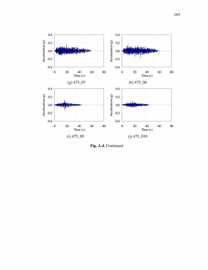
165

-0.4

-0.2

0.0

0.2

0.4

0 20 40 60 80Time (s)

Acc

eler

atio

n (g)

.

-0.4

-0.2

0.0

0.2

0.4

0 20 40 60 80Time (s)

Acc

eler

atio

n (g)

.

(g) 475_07 (h) 475_08

-0.4

-0.2

0.0

0.2

0.4

0 20 40 60 80Time (s)

Acc

eler

atio

n (g)

.

-0.4

-0.2

0.0

0.2

0.4

0 20 40 60 80Time (s)

Acc

eler

atio

n (g)

.

(i) 475_09 (j) 475_010


166

APPENDIX B MAXIMUM INTERSTORY DRIFTS

The maximum interstory drifts for both the 10% and 2% in 50 years hazards for

each case study for the Rix and Fernandez and the Wen and Wu ground motion records

are provided. The median maximum drifts are provided for each case in bold.

0

1

2

3

4

5

0 1 2 3


Sto

ry L

evel

475_01475_02475_03475_04475_05475_06475_07475_08475_09475_10Median

10% in 50 years

0

1

2

3

4

5

0 1 2 3 4 5 6 7 8


Sto

ry L

evel

2475_012475_022475_032475_042475_052475_062475_072475_082475_092475_10Median

2% in 50 years

(a) CS1

Fig. B.1. N-S maximum interstory drifts (Rix and Fernandez motions)

167

0

1

2

3

4

5

0 1 2 3Interstory Drift (%)

Sto

ry L

evel

475_01475_02475_03475_04475_05475_06475_07475_08475_09475_10Median

10% in 50 years

0

1

2

3

4

5

0 1 2 3 4 5 6 7 8Interstory Drift (%)

Sto

ry L

evel

2475_012475_022475_032475_042475_052475_062475_072475_082475_092475_10Median

2% in 50 years

(b) CS2

0

1

2

3

4

5


Sto

ry L

evel

475_01475_02475_03475_04475_05475_06475_07475_08475_09475_10Median

10% in 50 years

0

1

2

3

4

5

0 1 2 3 4 5 6 7 8Interstory Drift (%)

Sto

ry L

evel

2475_012475_022475_032475_042475_052475_062475_072475_082475_092475_10Median

2% in 50 years

(c) CS3

Fig. B.1. Continued.

168

0

1

2

3

4

5

0 1 2 3


Sto

ry L

evel

475_01475_02475_03475_04475_05475_06475_07475_08475_09475_10Median

10% in 50 years

0

1

2

3

4

5

0 2 4 6 8 10 12

Interstory Drift (%)S

tory

Lev

el

2475_012475_022475_032475_042475_052475_062475_072475_082475_092475_10Median

2% in 50 years

(a) CS1

0

1

2

3

4

5

0 1 2 3


Sto

ry L

evel

475_01475_02475_03475_04475_05475_06475_07475_08475_09475_10Median

10% in 50 years

0

1

2

3

4

5

0 2 4 6 8 10 12


Sto

ry L

evel

2475_012475_022475_032475_042475_052475_062475_072475_082475_092475_10Median

2% in 50 years

(b) CS2

Fig. B.2. E-W maximum interstory drifts (Rix and Fernandez motions)

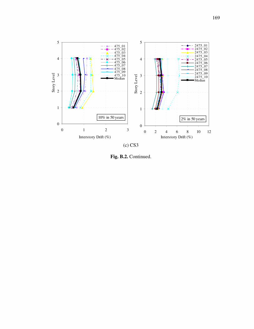
169

0

1

2

3

4

5

0 1 2 3


Sto

ry L

evel

475_01475_02475_03475_04475_05475_06475_07475_08475_09475_10Median

10% in 50 years

0

1

2

3

4

5

0 2 4 6 8 10 12


tory

Lev

el

2475_012475_022475_032475_042475_052475_062475_072475_082475_092475_10Median

2% in 50 years

(c) CS3


170

0

1

2

3

4

5


Sto

ry L

evel

475_01475_02475_03475_04475_05475_06475_07475_08475_09475_10Median

10% in 50 years

0

1

2

3

4

5

0 2 4 6 8 10 12


tory

Lev

el

2475_012475_022475_032475_042475_052475_062475_072475_082475_092475_10Median

2% in 50 years

(a) CS1

0

1

2

3

4

5


Sto

ry L

evel

475_01475_02475_03475_04475_05475_06475_07475_08475_09475_10Median

10% in 50 years

0

1

2

3

4

5

0 2 4 6 8 10 12


Sto

ry L

evel

2475_012475_022475_032475_042475_052475_062475_072475_082475_092475_10Median

2% in 50 years

(b) CS2

Fig. B.3. E-W maximum interstory drifts (Wen and Wu motions)

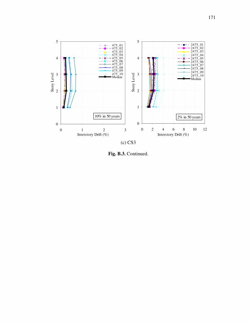
171

0

1

2

3

4

5


Sto

ry L

evel

475_01475_02475_03475_04475_05475_06475_07475_08475_09475_10Median

10% in 50 years

0

1

2

3

4

5

0 2 4 6 8 10 12


tory

Lev

el

2475_012475_022475_032475_042475_052475_062475_072475_082475_092475_10Median

2% in 50 years

(c) CS3


172

0

1

2

3

4

5


Sto

ry L

evel

475_01475_02475_03475_04475_05475_06475_07475_08475_09475_10Median

10% in 50 years

0

1

2

3

4

5

0 2 4 6 8 10 12


tory

Lev

el

2475_012475_022475_032475_042475_052475_062475_072475_082475_092475_10Median

2% in 50 years

(a) CS1

0

1

2

3

4

5


Sto

ry L

evel

475_01475_02475_03475_04475_05475_06475_07475_08475_09475_10Median

10% in 50 years

0

1

2

3

4

5

0 2 4 6 8 10 12


Sto

ry L

evel

2475_012475_022475_032475_042475_052475_062475_072475_082475_092475_10Median

2% in 50 years

(b) CS2

Fig. B.4. N-S maximum interstory drifts (Wen and Wu motions)

173

0

1

2

3

4

5


Sto

ry L

evel

475_01475_02475_03475_04475_05475_06475_07475_08475_09475_10Median

10% in 50 years

0

1

2

3

4

5

0 2 4 6 8 10 12


tory

Lev

el

2475_012475_022475_032475_042475_052475_062475_072475_082475_092475_10Median

2% in 50 years

(c) CS3


174

VITA

Name: Erin Kueht Address: Texas A&M University 3136 TAMU College Station, TX 77843-3136 Email Address: [email protected] Student Organizations: Structural Engineering Association of Texas, Texas A&M student chapter American Society of Civil Engineers, Texas A&M student chapter Education: B.S., Texas A&M University, Civil Engineering, 2004 M.S., Texas A&M University, Civil Engineering, 2007

impact of seismic code provisions in the central u.s.: a

Documents