impact of the optimum routing and least overhead routing approaches on minimum hop routes and...

8/7/2019 Impact of the Optimum Routing and Least Overhead Routing Approaches on Minimum Hop Routes and Connected …

http://slidepdf.com/reader/full/impact-of-the-optimum-routing-and-least-overhead-routing-approaches-on-minimum 1/17

International Journal of Wireless & Mobile Networks (IJWMN) Vol. 3, No. 2, April 2011

DOI : 10.5121/ijwmn.2011.3216 196

IMPACT OF THE OPTIMUM R OUTING AND LEAST

O VERHEAD R OUTING A PPROACHES ON MINIMUM

HOP R OUTES AND CONNECTED DOMINATING

SETS IN MOBILE A D HOC NETWORKS

Natarajan Meghanathan

Jackson State University, 1400 Lynch St, Jackson, MS, [email protected]

A BSTRACT

Communication protocols for mobile ad hoc networks (MANETs) follow either an Optimum Routing

Approach (ORA) or the Least Overhead Routing Approach (LORA): With ORA, protocols tend to

determine and use the optimal communication structure at every time instant; whereas with LORA, a protocol tends to use a chosen communication structure as long as it exists. In this paper, we study the

impact of the ORA and LORA strategies on minimum hop routes and minimum connected dominating sets

(MCDS) in MANETs. Our primary hypothesis is that the LORA strategy could yield routes with a larger

time-averaged hop count and MCDS node size when compared to the minimum hop count of routes and

the node size of the MCDS determined using the ORA strategy. Our secondary hypothesis is that the

impact of ORA vs. LORA also depends on how long the communication structure is being used. Our

hypotheses are evaluated using extensive simulations under diverse conditions of network density, node

mobility and mobility models such as the Random Waypoint model, City Section model and the

Manhattan model. In the case of minimum hop routes, which exist for relatively a much longer time

compared to the MCDS, the hop count of routes maintained according to LORA, even though not

dramatically high, is appreciably larger (6-12%) than those maintained according to ORA; on the other

hand, the number of nodes constituting a MCDS maintained according to LORA is only at most 6%

larger than the node size of a MCDS maintained under the ORA strategy.

K EYWORDS

Minimum hop routes, Minimum connected dominating sets, Optimum routing approach, Least overhead

routing approach, Mobile ad hoc networks, Simulations

1. INTRODUCTION

A mobile ad hoc network (MANET) is a dynamic distributed system of wireless nodes thatmove independently of each other. Routes in MANETs are often multi-hop in nature due to the

limited transmission range of the battery-operated wireless nodes. MANET routing protocolsare of two types [1][2]: proactive and reactive. Proactive routing protocols determine routes

between every pair of nodes in the network, irrespective of their requirement. Reactive or on-

demand routing protocols determine routes between any pair of nodes only if data needs to betransferred between the two nodes and no route is known between the two nodes. Proactive

routing protocols always tend to maintain optimum routes between every source-destination (s-

d ) pair and this strategy is called the Optimum Routing Approach (ORA) [1][3]. In this pursuit,each node periodically exchanges its routing table and link state information with other nodes in

the network, thus generating a significantly larger control overhead. On the other hand, reactiverouting protocols use a Least Overhead Routing Approach (LORA) [1][3] wherein an s-d route

is discovered through a global broadcast flooding-based route discovery process and the

discovered route is used as long as it exists. With node mobility, an s-d route determined to be




197

optimal at a particular time instant need not remain optimal in the subsequent time instants,even though the route may continue to exist. Thus, with LORA, it is possible that the routing

protocols continue to send data packets through sub-optimal routes. On the other hand, withORA, even though, we could send data packets at the best possible route at any time instant, thecost of periodically discovering such a route may be significantly high. In dynamically changing

network topologies, reactive on-demand routing protocols have been preferred over proactive

protocols with respect to the routing control overhead incurred [4][5].

From another perspective, among the routing algorithms and protocols proposed for MANETs,routing based on a connected dominating set (CDS) has been recognized as a suitable approach

in adapting quickly to the unpredictable fast-changing topology and dynamic nature of aMANET [6]. It is considered adaptable because as long as topological changes do not affect the

structure of the CDS, there is no need to reconfigure the CDS since the routing paths based on

the CDS would still be valid. A MANET is often represented as a unit disk graph [7] built of vertices and edges, where vertices signify nodes and edges signify bi-directional links that existbetween any two nodes if they are within each other’s transmission range. In a given graph

representing a MANET, a CDS is a dominating set within the graph whose induced sub graph isconnected. A dominating set of a graph is a vertex subset, such that every vertex is either in the

subset or adjacent to a vertex in the subset [8]. Routing based on a CDS within a MANET

means that routing control messages will be exchanged only amongst the CDS nodes and notbroadcast by all the nodes in the network; this will reduce the number of unnecessary

transmissions in routing [9].

There are multiple ways to form a CDS within a given MANET, and the algorithm used for

CDS formation will affect the performance and lifetime of the CDS and the performance of theMANET as a whole. A popular approach in CDS formation is attempting to form the smallest

possible CDS within a MANET, referred to as a minimum connected dominating set (MCDS).Reducing the size of the CDS will mean reducing the number of unnecessary transmissions.Unfortunately, the problem of determining a MCDS in an undirected graph like that of the unit

disk graph is NP-complete [9][12]. Efficient heuristics [10][11][12] have been proposed toapproximate the MCDS in wireless ad hoc networks. A common thread among these heuristics

is to give the preference of CDS inclusion to nodes that have high neighborhood density. TheMaxD-CDS heuristic [9] that we study in this paper is one such heuristic.

The objective of this paper is to study the impact of adopting the ORA and LORA strategies on

minimum hop routes and the node size of the MCDS in MANETs. Minimum hop routing is a

very widely adopted route selection principle of MANET routing protocols, belonging to bothproactive and reactive categories. Likewise, the primary objective of a majority of the MCDS-

based heuristics is to minimize the number of nodes constituting the CDS. As ORA determines

the best optimal route at any time instant, our primary hypothesis is that the hop count of

minimum hop routes and the node size of MCDS discovered under the LORA strategy would begreater than those discovered under the ORA strategy. Our secondary hypothesis is that the

impact of ORA vs. LORA also depends on how long the communication structure is being used.

We determine the percentage difference in the hop count of minimum hop s-d paths and the

node size of the MCDS determined under the two strategies. We conduct extensive simulationsunder three different network densities and three different mobility models with three differentlevels of node mobility. The three mobility models [13] used are the Random Waypoint model,

City Section model and Manhattan model. Even though performance comparison studies of individual proactive vs. reactive routing protocols as well as the different CDS algorithms are

available in the literature, an extensive simulation based analysis on the impact of the ORA andLORA strategies on the minimum hop count of routes and the node size of the MCDS

algorithms has not been conducted in the literature and therein lies our contribution through this

paper.




198

The rest of the paper is organized as follows: Section 2 discusses the algorithms employed fordetermining minimum hop routes under the ORA and LORA strategies and also illustrates an

example highlighting the difference between the two strategies and their impact on the hopcount of s-d paths. Section 3 discusses the algorithms employed for determining MCDS underthe ORA and LORA strategies and also illustrates an example highlighting the difference

between the two strategies and their impact on the node size of the MCDS. Section 4 reviews

the three different mobility models used in the simulations. Section 5 describes the simulation

environment and presents the simulation results for hop count per s-d path, node size perMCDS, path lifetime and network connectivity. Section 6 concludes the paper and lists future

work. Throughout the paper, the terms ‘node’ and ‘vertex’, ‘edge’ and ‘link’, ‘path’ and ‘route’are used interchangeably. They mean the same.

2. DETERMINATION OF MINIMUM HOP ROUTES UNDER THE ORA AND

LORA STRATEGIES

We use the notion of a mobile graph [14] defined as the sequence G M = G1G2 … GT of static

graphs that represent the network topology changes over the time scale T , representing thesimulation time. We sample the network topology periodically, for every 0.25 seconds, which in

reality could be the instants of data packet origination at the source. Each of the static graphs isa unit disk graph [7] of nodes and edges, wherein there exists an edge if and only if the

Euclidean distance between the two constituent end nodes of the edge is within the transmissionrange of the nodes. We assume every node operates at a fixed transmission range, R.

For the ORA strategy, we determine the sequence of minimum hop s-d paths between a source

node s and a destination node d by running the Breadth First Search (BFS) algorithm [15],starting from the source node s, on each of the static graphs of the mobile graph generated over

the entire time period of the simulation. In the case of LORA, if we do not know a path fromsource s to destination d in static graph Gi, we run BFS (pseudo code in Figure 1), starting from

node s, on Gi and determine the minimum hop path Ps-d from s to d . For subsequent static graphs

Gi+1, Gi+2, …, we simply test the presence of path Ps-d . We validate the existence of a path Ps-d instatic graph G j by testing the existence of every constituent edge of Ps-d in G j. If every

constituent edge of Ps-d exists in G j, then the path Ps-d exists in G j. Otherwise, we run BFS on G j,starting from the source node s, and determine a new s-d path Ps-d . This procedure is repeateduntil the end of the simulation time. The pseudo code of our algorithms to determine the

minimum hop paths under the ORA and LORA strategies is given in Figures 2 and 3

respectively.

Input: Static Graph G = (V , E ), source node s, destination node d Auxiliary Variables/Initialization: Nodes-Explored = Φ, FIFO-Queue = Φ

∀ node v∈V , Parent (v) = NULLBegin Algorithm BFS (G, s, d)

Nodes-Explored = Nodes-Explored U {s}FIFO-Queue = FIFO-Queue U {s}while ( |FIFO-Queue| > 0 ) do

node u = Dequeue(FIFO-Queue) // extract the first nodefor (every edge (u, v) ) do // i.e. every neighbor v of node u

if ( v ∉ Nodes-Explored ) then

Nodes-Explored = Nodes-Explored U {v}

FIFO-Queue = FIFO-Queue U {v}Parent (v) = u

end if

end for




199

end whileif ( | Nodes-Explored | = | V | ) then

Path Pd-s = {d }temp-node = d while (Parent (temp-node) != NULL) do

Pd-s = Pd-s U {Parent (temp-node)}

temp-node = Parent (temp-node)

end whilePath Ps-d = reverse(Pd-s)return Ps-d

end if

else

return NULL // no s-d path

end if End Algorithm BFS

Figure 1: Breadth First Search (BFS) Algorithm to Determine Minimum Hop s-d Path

Input: G M = G1G2 … GT , source s, destination d Auxiliary Variable: i, Path Ps-d

Initialization: i=1; Ps-d = NULL

Begin ORA-MinHopPathswhile (i ≤ T ) do

Path Ps-d = BFS(Gi, s, d )

i = i + 1

end whileEnd ORA-MinHopPaths

Figure 2: Pseudo Code to Find a Sequence of Minimum Hop s-d Paths under the ORA Strategy

Input: G M = G1G2 … GT , source s, destination d Auxiliary Variables: i, j, Path Ps-d Initialization: i=1; j=1; Ps-d = NULLBegin LORA-MinHopPaths

while (i ≤ T ) do

if (Ps-d != NULL) then

for every edge (u, v) in Ps-d doif ( (u, v) does not exist in Gi) then

Ps-d = NULL

end if

end for

end if

if (Ps-d = NULL) then Path Ps-d = BFS(Gi, s, d )

end if i = i + 1

end whileEnd LORA-MinHopPaths

Figure 3: Pseudo Code to Find Sequence of Minimum Hop s-d Paths under the LORA Strategy




200

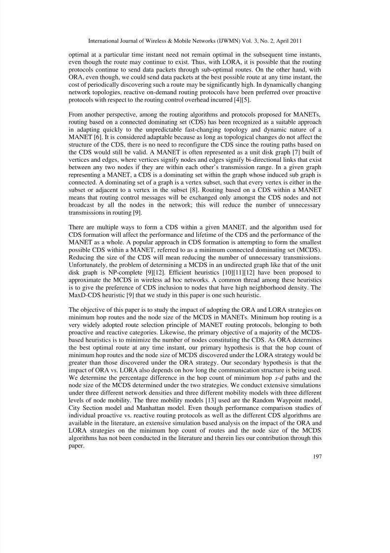
Figure 4: Example to Illustrate the ORA and LORA Strategies for Minimum Hop Routing

Figure 4 is an example to illustrate the difference between the ORA and LORA strategies withrespect to minimum hop routing. We sample the network topology for five consecutive instants

of time as shown. The source and destination node IDs are 1 and 4 respectively. We notice that

under the LORA strategy, we could use path {1 – 2 – 4 – 5} for time instants t 1 and t 2 and path{1 – 7 – 2 – 4} for time instants t 3, t 4 and t 5 respectively. The paths {1 – 2 – 4 – 5} and {1 – 7 –

2 – 4} appear to be the best possible minimum hop paths at the time of discovery, i.e., at time

instants t 1 and t 3 respectively. Nevertheless, after each of these paths is chosen at a particulartime instant, we notice the emergence of relatively shorter paths (i.e., with a lower hop count) in

the static graphs captured at subsequent time instants. But it is not possible to use these paths

under the LORA strategy. With ORA, the strategy is to capture the minimum hop paths at everytime instant.

3. DETERMINATION OF MINIMUM CONNECTED DOMINATING SETS UNDER

THE ORA AND LORA STRATEGIES

The algorithm used to approximate a MCDS is referred to as the MaxD-CDS algorithm [9] as it

prefers to include nodes that have a larger number of uncovered neighbors (density) to be part of the CDS. The MaxD-CDS algorithm uses the following principal data structures:

(i) CDS-Node-List – includes all nodes that are members of the CDS(ii) Covered-Nodes-List – includes all nodes that are in the CDS-Node-List and all nodes

that are adjacent to at least one member of the CDS-Node-List.

Before we run the MaxD-CDS algorithm, we make sure the underlying network graph isconnected by running the Breadth First Search (BFS) algorithm [15]; because, if the underlying

network graph is not connected, we would not be able to find a CDS that will cover all thenodes in the network. We run BFS, starting with an arbitrarily chosen node in the network

graph. If we are able to visit all the vertices in the graph, then the corresponding network is saidto be connected. If the graph is not connected, we simply collect a snapshot of the network topology at the next time instant and start with the BFS test. The pseudo code for the BFS

algorithm is given in Figure 5.




201

Input: Graph G = (V , E )Auxiliary Variables/Initialization: Nodes-Explored = Φ, FIFO-Queue = Φ Begin Algorithm BFS (G, s)

root-node = randomly chosen vertex in V

Nodes-Explored = Nodes-Explored U {root-node}FIFO-Queue = FIFO-Queue U {root-node}

while ( |FIFO-Queue| > 0 ) do

front-node u = Dequeue(FIFO-Queue) // extract the first node

for (every edge (u, v) ) do // i.e. every neighbor v of node u

if ( v ∉ Nodes-Explored ) then

Nodes-Explored = Nodes-Explored U {v}FIFO-Queue = FIFO-Queue U {v}

Parent (v) = u

end if

end for

end while

if ( | Nodes-Explored | = | V | ) then return Connected Graph - trueelse return Connected Graph - false

end if End Algorithm BFS

Figure 5: Modified BFS Algorithm to Test for Graph Connectivity

The MaxD-CDS algorithm (pseudo code in Figure 6) outputs a CDS-Node-List based on a given

input MANET graph. The first node to be included in the CDS-Node-List is the node with the

maximum number of uncovered neighbors (any ties are broken arbitrarily). A CDS member isconsidered to be “covered”, so a CDS member is additionally added to the Covered-Nodes-List

as it is added to the CDS-Node-List . All nodes that are adjacent to a CDS member are also saidto be covered, so the uncovered neighbors of a CDS member are also added to the Covered-

Nodes-List as the member is added to the CDS-Node-List . To determine the next node to beadded to the CDS-Node-List , we must select the node with the largest density amongst the nodes

that meet the criteria for inclusion into the CDS. The criteria for CDS membership selection arethe following: the node cannot already be a part of the CDS (CDS-Node-List), the node must be

in the Covered-Nodes-List , and the node must have at least one uncovered neighbor (at least one

neighbor that is not in the Covered-Nodes-List ). Amongst the nodes that meet these criteria forCDS membership inclusion, we select the node with the largest density (i.e., the largest number

of uncovered neighbors) to be the next member of the CDS. Ties are broken arbitrarily. This

process is repeated until all nodes in the network are included in the Covered-Nodes-List . Onceall nodes in the network are considered to be “covered”, the CDS has been formed and the

algorithm returns a list of the members included in the resultant MaxD-CDS (nodes in the CDS-

Node-List ).

Input: Graph G = (V , E ); V – vertex set, E – edge set

Source vertex, s – vertex with the largest number of uncovered neighbors in V Auxiliary Variables and Functions: CDS-Node-List , Covered-Nodes-List, Neighbors(v) for

every v in V Output: CDS-Node-List Initialization: Covered-Nodes-List = {s}, CDS-Node-List = Φ

Begin Construction of MaxD-CDS (G, s) while ( |Covered-Nodes-List | < |V | ) do




202

Select a vertex r ∈Covered-Nodes-List and r ∉CDS-Node-List such that r has the largest

number of uncovered neighbors that are not in Covered-Nodes-List

CDS-Node-List = CDS-Node-List U {r }

for all u∈ Neighbors(r ) and u∉Covered-Nodes-List

Covered-Nodes-List = Covered-Nodes-List U {u}

end forend while

return CDS-Node-List

End Construction of MaxD-CDS

Figure 6: Pseudo Code for the Algorithm to Construct Maximum Density (MaxD)-based CDS

For the ORA strategy, we determine the sequence of MCDS by running the MaxD-CDSalgorithm, starting from the source node s – the node with the largest number of neighbors, on

each of the static graphs of the mobile graph generated over the entire time period of thesimulation. In the case of LORA, if we do not know a MCDS in static graph Gi, we run the

MaxD-CDS algorithm, starting from the source node s – the node with the largest number of neighbors in Gi and determine the MCDS. For subsequent static graphs Gi+1, Gi+2, …, we simply

test the presence of the MCDS. We validate a MCDS in a static graph G j by first testing the

connectivity among the nodes that constitute the MCDS and then testing whether each non-MCDS node in G j is a neighbor of at least one node in the MCDS. If both these tests return true,

then we consider the MCDS to exist in G j. Otherwise, we run the MaxD-CDS algorithm on G j,

starting from a source node s – the node with the largest number of neighbors in G j anddetermine a new MCDS. This procedure is repeated until the end of the simulation time. A

pseudo code for the algorithm to validate a MCDS is given in Figure 7. The pseudo code of our

algorithms to determine the MCDS under the ORA and LORA strategies is given in Figures 8and 9 respectively.

Input: CDS-Node-List // Set of vertices part of the CDS

Auxiliary Variables and Functions:CDS-Edge-List – Set of edges, ⊆ E , between the vertices that are part of CDS-Node-List

connectedCDS – Boolean variable that stores information whether CDS-Node-List andCDS-Edge-List form a connected sub graph of G.

Output: true or false // true, if the nodes in CDS-Node-List form a connected sub graph of G and every vertex

v∉CDS-Node-List is a neighbor of a vertex u∈CDS-Node-List

// false, if the nodes in CDS-Node-List do not form a connected sub graph of G and/or

there exists at least one vertex v∉CDS-Node-List that has no neighbor in CDS-Node-List

Initialization: CDS-Edge-List = Φ Begin CDS-Validation (CDS-Node-List , time instant t )

for every pair of vertices u, v ∈CDS-Node-List do

if there exists an edge (u, v)∈ E at time instant t thenCDS-Edge-List = CDS-Edge-List U {(u, v)}

end if

end forconnectedCDS = Breadth-First-Search(CDS-Node-List , CDS-Edge-List )

if connectedCDS = true then

for every vertex v∉CDS-Node-List do

if there exists no edge (u, v)∈ E where u∈CDS-Node-List at time instant t then




203

return false

end if

end for

return true

end if

return false // if connectedCDS = false

End CDS-Validation

Figure 7: Pseudo Code for the CDS Validation Algorithm

Input: G M = G1G2 … GT Auxiliary Variable: i, MCDSi

Initialization: i=1; MCDSi = NULL

Begin ORA-MCDS

while (i ≤ T ) do

Choose the source node s – the node with the largest number of neighbors in Gi if BFS (Gi , s) returns true

MCDSi = MaxD-CDS(Gi, s)

end if i = i + 1

end whileEnd ORA-MCDS

Figure 8: Pseudo Code to Determine a Sequence of MCDS under the ORA Strategy

Input: G M = G1G2 … GT , source s, destination d

Auxiliary Variables: i, j, MCDS Initialization: i=1; j=1; MCDS = NULL

Begin LORA-MCDS

while (i ≤ T ) do

if ( MCDS != NULL) then

if ( CDS-Validation (CDS-Node-List of MCDS, time instant i) returns false) then

MCDS = NULL

end if

end if if ( MCDS = NULL) then

Choose the source node s – the node with the largest number of neighbors in Gi if BFS (Gi , s) returns true

MCDS = MaxD-CDS(Gi, s)

end if end if

i = i + 1

end while

End LORA-MCDS

Figure 9: Pseudo Code to Determine Minimum Hop s-d Paths under the LORA Strategy




204

Figure 10: Example to Illustrate the ORA and LORA Strategies for Determining MCDS

Figure 10 is an example to illustrate the difference between the ORA and LORA strategies with

respect to determining MCDS. We sample the network topology for five consecutive instants of

time as shown. To determine a MCDS on a particular network topology, we start with the vertex(node ID 2 in all the cases) that has the largest number of neighbors. While deciding whether a

covered node can be part of the CDS-Node-List of the MCDS, we include the covered node with

the largest number of uncovered neighbors. Any tie in this case is broken in favor of the covered

node that has the lowest ID. We notice that under the LORA strategy, we could use the MCDScomprising of nodes {2, 1, 5} with edges {1 – 2, 2 – 5} for time instants t 1 and t 2 and the MCDS

comprising of nodes {2, 4, 7} with edges {2 – 4, 2 – 7} for time instants t 3, t 4 and t 5 respectively. The average MCDS node size under the LORA approach is 3.0 as there are three

nodes in the MCDS used in each of the five time instants. On the other hand, under the ORAstrategy, we determine MCDS comprising of nodes {2, 1, 5}, {2, 1}, {2, 4, 7}, {2, 4}, {2, 4} at

time instants t 1, t 2, t 3, t 4 and t 5 respectively. Hence, the average MCDS node size is 2.4. Noticethat the absence of link 2 – 1 in the graph at time instant t 3 forced us to choose the MCDS with

nodes {2, 4, 7} at t 3; once this link appears at time instants t 4 and t 5, by adopting the ORA

strategy – we could reduce the number of nodes in the MCDS from three to two; whereas, byadopting the LORA strategy, we end up continuing to stay with a MCDS comprising of three

nodes. Updating the MCDS for every time instant helps to reduce the number of constituent

CDS nodes; however, with a significant control overhead. Using a CDS with a larger number of constituent nodes leads to redundant retransmissions in the case of flooding using the CDS. This

illustrates the difference and trade off between the ORA and LORA strategies.

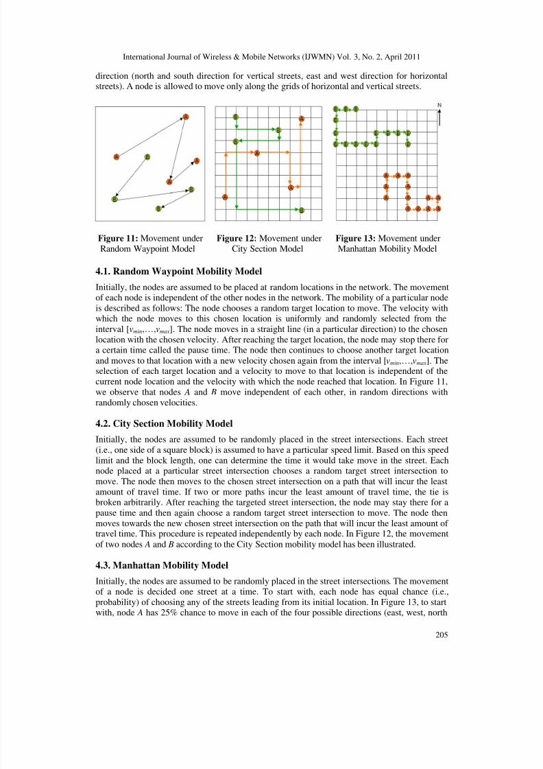
4. REVIEW OF MOBILITY MODELS

All the three mobility models assume the network is confined within fixed boundary conditions.The Random Waypoint mobility model assumes that the nodes can move anywhere within a

network region. The City Section and the Manhattan mobility models assume the network to be

divided into grids: square blocks of identical block length. The network is thus basicallycomposed of a number of horizontal and vertical streets. Each street has two lanes, one for each




205

direction (north and south direction for vertical streets, east and west direction for horizontalstreets). A node is allowed to move only along the grids of horizontal and vertical streets.

Figure 11: Movement under Figure 12: Movement under Figure 13: Movement underRandom Waypoint Model City Section Model Manhattan Mobility Model

4.1. Random Waypoint Mobility Model

Initially, the nodes are assumed to be placed at random locations in the network. The movementof each node is independent of the other nodes in the network. The mobility of a particular node

is described as follows: The node chooses a random target location to move. The velocity withwhich the node moves to this chosen location is uniformly and randomly selected from the

interval [vmin,…,vmax]. The node moves in a straight line (in a particular direction) to the chosen

location with the chosen velocity. After reaching the target location, the node may stop there fora certain time called the pause time. The node then continues to choose another target location

and moves to that location with a new velocity chosen again from the interval [vmin,…,vmax]. Theselection of each target location and a velocity to move to that location is independent of the

current node location and the velocity with which the node reached that location. In Figure 11,

we observe that nodes A and B move independent of each other, in random directions with

randomly chosen velocities.

4.2. City Section Mobility Model

Initially, the nodes are assumed to be randomly placed in the street intersections. Each street

(i.e., one side of a square block) is assumed to have a particular speed limit. Based on this speed

limit and the block length, one can determine the time it would take move in the street. Eachnode placed at a particular street intersection chooses a random target street intersection to

move. The node then moves to the chosen street intersection on a path that will incur the least

amount of travel time. If two or more paths incur the least amount of travel time, the tie isbroken arbitrarily. After reaching the targeted street intersection, the node may stay there for a

pause time and then again choose a random target street intersection to move. The node then

moves towards the new chosen street intersection on the path that will incur the least amount of travel time. This procedure is repeated independently by each node. In Figure 12, the movement

of two nodes A and B according to the City Section mobility model has been illustrated.

4.3. Manhattan Mobility Model

Initially, the nodes are assumed to be randomly placed in the street intersections. The movementof a node is decided one street at a time. To start with, each node has equal chance (i.e.,

probability) of choosing any of the streets leading from its initial location. In Figure 13, to startwith, node A has 25% chance to move in each of the four possible directions (east, west, north




206

or south), where as node B can move only either to the west, east or south with a 1/3 chance foreach direction. After a node begins to move in the chosen direction and reaches the next street

intersection, the subsequent street in which the node will move is chosen probabilistically. If anode can continue to move in the same direction or can also change directions, then the nodehas 50% chance of continuing in the same direction, 25% chance of turning to the east/north and

25% chance of turning to the west/south, depending on the direction of the previous movement.

If a node has only two options, then the node has an equal (50%) chance of exploring either of

the two options. For example, in Figure 13, once node A reaches the rightmost boundary of thenetwork, the node can either move to the north or to the south, each with a probability of 0.5

and the node chooses the north direction. After moving to the street intersection in the north,node A can either continue to move northwards or turn left and move eastwards, each with a

probability of 0.5. If a node has only one option to move (this occurs when the node reaches any

of the four corners of the network), then the node has no other choice except to explore thatoption. For example, in Figure 13, we observe node B that was traveling westward, reaches thestreet intersection, which is the corner of the network. The only option for node B is then to turn

to the left and proceed southwards.

5. SIMULATIONS

Simulations have been conducted in a discrete-event simulator implemented by the author inJava. Network dimensions are 1000m x 1000m. For the Random Waypoint mobility model, we

assume the nodes can move anywhere within the network. For the City Section and Manhattanmobility models, we assume the network is divided into grids: square blocks of length (side)

100m. The network is thus basically composed of a number of horizontal and vertical streets.Each street has two lanes, one for each direction (north and south direction for vertical streets,

east and west direction for horizontal streets). A node is allowed to move only along the grids of horizontal and vertical streets. The wireless transmission range of a node is 250m. The network

density is varied by performing the simulations with 50 (low density), 100 (moderate density)and 150 (high density) nodes. The node velocity values used for each of the three mobility

models are 2.5 m/s (about 5 miles per hour), 12.5 m/s (about 30 miles per hour) and 25 m/s(about 60 miles per hour), representing scenarios of low, moderate and high node mobilityrespectively. For the Random Waypoint mobility model, we assume vmin = vmax.

We obtain a centralized view of the network topology by generating mobility trace files for1000 seconds under each of the three mobility models. The network topology is sampled for

every 0.25 seconds to generate the static graphs and the mobile graph. Two nodes a and b areassumed to have a bi-directional link at time t , if the Euclidean distance between them at time t

(derived using the locations of the nodes from the mobility trace file) is less than or equal to thewireless transmission range of the nodes. Each data point in Figures 14 through 19 and in

Tables 1 to 6 is an average computed over 5 mobility trace files and 20 randomly selected s-d

pairs from each of the mobility trace files. The starting time of each s-d session is uniformlydistributed between 1 to 20 seconds.

The following performance metrics are evaluated:

• Percentage Network Connectivity: The percentage network connectivity indicates the

probability of finding an s-d path between any source s and destination d in networks for agiven density and a mobility model. Measured over all the s-d sessions of a simulation run,

this metric is the ratio of the number of static graphs in which there is an s-d path to the total

number of static graphs in the mobile graph.

• Average Route Lifetime: The average route lifetime is the average of the lifetime of all the

static paths of an s-d session, averaged over all the s-d sessions.

• Average Hop Count : The average hop count is the time averaged hop count of a mobile path

for an s-d session, averaged over all the s-d sessions. The time averaged hop count for an s-




207

d session is measured as the sum of the products of the number of hops per static s-d pathand the lifetime of the static s-d path divided by the number of static graphs in which there

existed a static s-d path. For example, if a mobile path spanning over 10 static graphscomprises of a 2-hop static path p1, a 3-hop static path p2, and a 2-hop static path p3, witheach existing for 2, 3 and 5 seconds respectively, then the time-averaged hop count of the

mobile path would be (2*2 + 3*3 + 2*5) / 10 = 2.3.

• CDS Node Size: This is a time-averaged value of the number of nodes included in the

sequence of minimum connected dominating sets used over the entire duration of the

simulation.

Figure 14: % Connectivity (vel = 2.5 m/s) Figure 15: Lifetime per s-d Path (vel = 2.5 m/s)

Figure 16: % Connectivity (vel = 12.5 m/s) Figure 17: Lifetime per s-d Path (vel = 12.5 m/s)

Figure 18: % Connectivity (vel = 25 m/s) Figure 19: Lifetime per s-d Path (vel = 25 m/s)

5.1. Network Connectivity

The percentage network connectivity (refer Figures 14, 16 and 18) is not dependent on therouting strategy (ORA or LORA) and is dependent only on the mobility model, the level of

node mobility and network density. It is quite natural to observe that for a given mobility modeland level of node mobility, the percentage network connectivity increases with increase innetwork density. In low density networks (50 nodes), the Random Waypoint model provided the

largest network connectivity for a given level of node mobility; the City Section and Manhattan

models yielded a relatively lower network connectivity, differing as large as by 11% . This canbe attributed to the constrained motion of the nodes only along the streets of the network. On

the other hand, as we increase the network density (100 node scenarios), the City Section model

and/or the Manhattan model yielded network connectivity equal or larger than that incurred withthe Random Waypoint model. As more nodes are added to the streets, the probability of finding




208

source-destination routes at any point of time increases significantly. It is also interesting toobserve that for a given network density, the network connectivity provided by each of the three

mobility models almost remained the same for different values of node velocity. Hence,network connectivity is mainly influenced by the number of nodes in the network and theirinitial random distribution. The randomness associated with the mobility models ensure that

node velocity is not a significant factor influencing network connectivity.

5.2. Route Lifetime

The average route lifetime (Figures 15, 17 and 19) is measured only for routes discovered under

the LORA strategy as routes are determined for every static graph under the ORA strategy. WithLORA, a route is used as long as it exists. The average route lifetime of minimum hop routes is

mainly influenced by node velocity and to a lesser extent by the mobility model and network density, in this order. For a given node velocity and network density, minimum hop routes

determined under the City Section model had the largest lifetime and those determined under

the Manhattan model had the smallest lifetime except the scenario of 100 nodes with 12.5 m/svelocity, wherein the Random Waypoint model yielded routes with the lowest average lifetime.

For a given node velocity, the difference in the average lifetime of routes between the City

Section model and the other two mobility models increase with increase in network density. The

City Section model yielded a route lifetime that is 8-20% and 17-26% more than that discoveredunder the Random Waypoint model in low and high density networks respectively. Compared

to the Manhattan model, the City Section model yielded routes that have 15-30% and 12-35%larger lifetime in low and high density networks respectively. For a given mobility model, the

route lifetime seem to decrease proportionately with increase in node velocity. As we increasethe node velocity from 2.5 m/s to 25 m/s, the average lifetime of minimum hop routes

determined under a particular mobility model approximately reduced to 1/10th

of their value atlow node velocity.

5.3. Hop Count of Minimum Hop Routes

For each mobility model, node velocity and network density, we observe that minimum hop

routes discovered under the LORA strategy has a larger hop count than those discovered under

the ORA strategy. But, the increase in the hop count is not substantial and is within 12%. Thisindicates that if the on-demand MANET routing protocols based on the LORA strategy aredesigned meticulously with minimum hop routing as the primary routing principle, they could

discover routes that have at most 12% larger hop count than those discovered by the ORA-basedproactive routing protocols. Among the three mobility models, the maximum increase in the hop

count under the LORA strategy vis-à-vis the ORA strategy is observed with the RandomWaypoint model and the lowest increase in the hop count is observed with the Manhattan

model. However, with regards to the absolute values of the hop count, the minimum hop routes

determined under the Random Waypoint model have the smallest hop count and thosedetermined under the Manhattan model have the largest hop count.

For a given mobility model, the hop count of the minimum hop routes determined for a

particular network density does not seem to be much influenced with different levels of node

mobility. For a given mobility model and node velocity, we also observe that under both theORA and LORA strategies, the average hop count of minimum hop routes decreases with

increase in network density. This can be attributed to the reasoning that with a larger number of nodes in the network, there is a larger probability of finding an s-d path involving only fewer

nodes that lie on the path from the source to the destination. The decrease in the hop count of minimum hop routes with increase in network density is very much appreciable for the

Manhattan model compared to the other two mobility models.




209

Another interesting observation is that for a given network density, the percentage increase inthe average hop count per minimum hop s-d path decreases with increase in node mobility. This

can be attributed to significant decrease in the lifetime of the s-d routes with increase in nodemobility. At higher node mobility, the sub-optimal routes do not exist for a longer time and thesequence of routes determined under the LORA strategy starts getting closer to the sequence of

routes determined under the ORA strategy. This effect is more predominant in the case of

MCDS as the lifetime per CDS under the LORA strategy is significantly smaller than the

lifetime per s-d path.

Table 1: Average Hop Count per s-d Path under Random Waypoint Mobility Model

NodeVelocity

50 Node Network 100 Node Network 150 Node Network

ORA LORAPercentIncrease



2.5 m/s 2.36 2.63 11.51% 2.27 2.50 10.40% 2.21 2.43 9.95%

12.5 m/s 2.40 2.65 10.14% 2.36 2.58 9.46% 2.25 2.46 9.33%

25 m/s 2.40 2.63 9.44% 2.31 2.52 9.31% 2.24 2.44 8.93%

Table 2: Average Hop Count per s-d Path under City Section Mobility Model

Node

Velocity


ORA LORAPercent

IncreaseORA LORA

Percent

IncreaseORA LORA

Percent

Increase

2.5 m/s 2.66 2.86 7.51% 2.45 2.71 10.40% 2.24 2.50 11.60%

12.5 m/s 2.85 3.07 7.66% 2.70 2.93 8.68% 2.55 2.80 9.80%

25 m/s 2.83 3.04 7.39% 2.60 2.82 8.47% 2.37 2.60 9.70%

Table 3: Average Hop Count per s-d Path under Manhattan Mobility Model

Node

Velocity


ORA LORA

Percent

Increase ORA LORA

Percent

Increase ORA LORA

Percent

Increase2.5 m/s 3.31 3.60 8.81% 3.08 3.34 8.38% 2.75 3.03 10.12%

12.5 m/s 3.37 3.60 6.90% 3.00 3.26 8.60% 2.67 2.93 9.82%

25 m/s 3.51 3.74 6.60% 3.03 3.27 7.94% 2.52 2.76 9.35%

5.4. Node Size per Minimum Connected Dominating Sete

For each mobility model, the average node size per MCDS determined under the LORAstrategy is slightly higher than that determined under the ORA strategy. But, the increase is very

minimal and is only within 6%. This implies that the number of retransmissions incurred byadopting the sequence of MCDS determined under the LORA strategy will not be substantially

higher than those incurred using the sequence of MCDS determined under the ORA strategy.

On the other hand, there would be a significant control overhead in updating the MCDS for

every time instant. Hence, the LORA strategy could always be the preferred strategy todetermine and use MCDS in MANETs.

With respect to the absolute magnitude of the MCDS Node Size under the three mobilitymodels, we observe that the MCDS Node Size determined under the Random Waypoint model

is always the smallest and the MCDS Node Size determined under the Manhattan mobility

model is always the largest under the different conditions of node mobility and network density.The MCDS Node Size determined under the City Section mobility model is 16%, 20%-25% and




210

22%-24% larger than that determined under the Random Waypoint model in conditions of low,moderate and high network density respectively. The MCDS Node Size determined under the

Manhattan mobility model is 26%-36%, 31%-34% and 30%-34% larger than that determinedunder the Random Waypoint model in conditions of low, moderate and high network densityrespectively.

Table 4: Average Node Size per MCDS under Random Waypoint Mobility Model

NodeVelocity


ORA LORAPercent

IncreaseORA LORA

Percent

IncreaseORA LORA

Percent

Increase

2.5 m/s 9.80 10.12 3.27% 10.17 10.62 4.47% 10.09 10.65 5.55%

12.5 m/s 9.88 10.23 3.52% 9.93 10.24 3.12% 10.41 10.75 3.25%

25 m/s 9.54 9.94 4.19% 9.81 10.15 3.47% 10.21 10.51 2.93%

Table 5: Average Node Size per MCDS under City Section Mobility Model

Node

Velocity


ORA LORA PercentIncrease



2.5 m/s 11.43 11.78 3.06% 12.18 12.62 3.61% 12.58 13.07 3.89%

12.5 m/s 11.37 11.79 3.69% 12.18 12.65 3.86% 12.91 13.31 3.09%

25 m/s 11.15 11.47 2.87% 12.22 12.46 1.96% 12.68 12.91 1.81%

Table 6: Average Node Size per MCDS under Manhattan Mobility Model

Node

Velocity





2.5 m/s 12.42 12.89 3.78% 13.33 13.61 2.10% 13.53 13.95 3.10%

12.5 m/s 12.90 13.42 4.03% 13.34 13.76 3.15% 13.58 13.98 2.94%

25 m/s 13.01 13.32 2.38% 13.11 13.39 2.14% 13.45 13.73 2.08%

As observed in the case of minimum hop routes, for a given network density, the percentage

increase in the MCDS Node Size decreases with increase in node mobility. This can beattributed to the decrease in the MCDS lifetime by factors of 4 to 5 and 8 to 9 with increase in

the node velocity from 2.5 m/s to 12.5 m/s and 25 m/s respectively. For a given condition of

node mobility and network density, the lifetime per MCDS is only 1/3rd

to 1/4th

of the lifetimeper s-d path determined under similar conditions. Hence, compared to the minimum hop routes,

the CDS-Node-List of the sequence of MCDS formed under the LORA strategy fast coincides

with that of the sequence of MCDS formed under the ORA strategy.

6. CONCLUSIONS AND FUTURE WORK

Our hypothesis that there would be difference in the hop count of minimum hop routes and thenode size of the minimum connected dominating sets (MCDS) discovered under the ORA and

LORA strategies has been observed to be true through extensive simulations, the results of which are summarized in Tables 1 through 6. However, the difference is not significantly high

and is within 6-12% for minimum hop routes and at most 6% for MCDS, depending mainly on

the mobility model employed and the level of node mobility and to a lesser extent on thenetwork density. With respect to absolute values, the Random Waypoint model yields minimum

hop routes with the smallest hop count and MCDS with the smallest node size; whereas, the




211

Manhattan model yields minimum hop routes with the largest hop count and MCDS with thelargest node size. With respect to the increase in the hop count of minimum hop routes due to

the use of LORA strategy vis-à-vis the ORA strategy, we observe that the Random Waypointmodel incurs the maximum increase and the Manhattan model incurs the smallest increase. TheCity Section model is ranked in between the two mobility models with regards to the absolute

value of the hop count and the relative increase in the hop count with the LORA strategy. In the

context of the MCDS, the percentage increase in the number of nodes per MCDS due to the use

of LORA vis-à-vis ORA is about the same for all the three mobility models. With regards to theroute lifetime, the minimum hop routes determined under the City Section model are relatively

more stable (i.e. have larger lifetime) compared to the other two mobility models.

Another interesting observation is that for a given network density, the percentage increase in

the average hop count per minimum s-d path and the number of nodes per MCDS decreases

with increase in node mobility. This can be attributed to the significant decrease in the lifetimeof the s-d routes and the MCDS with increase in node mobility. This effect is more predominantin the case of MCDS as the lifetime per MCDS under the LORA strategy is significantly

smaller than the lifetime per s-d path. Hence, compared to the minimum hop routes, the CDS-

Node-List of the sequence of MCDS formed under the LORA strategy fast coincides with that

of the sequence of MCDS formed under the ORA strategy. As future work, we will be

extending this study and will examine the impact of the ORA vs. LORA strategies and the threemobility models on minimum-hop based multicast routing, minimum-link based multicast

Steiner trees, as well as node-disjoint and link-disjoint multi-path routing for MANETs.

REFERENCES

[1] M. Abolhasan, T. Wysocki and E. Dutkiewicz, “A Review of Routing Protocols for Mobile Ad hoc

Networks,” Ad hoc Networks, vol. 2, no. 1, pp. 1-22, January 2004.

[2] N. Meghanathan, “Survey and Taxonomy of Unicast Routing Protocols for Mobile Ad hoc

Networks,” The International Journal on Applications of Graph Theory in Wireless Ad hoc Networks

and Sensor Networks, vol. 1, no. 1, pp. 1-21, December 2009.

[3] C. Siva Ram Murthy and B. S. Manoj, “Routing Protocols for Ad Hoc Wireless Networks,” Ad Hoc

Wireless Networks: Architectures and Protocols, Chapter 7, Prentice Hall, June 2004.[4] J. Broch, D. A. Maltz, D. B. Johnson, Y. C. Hu and J. Jetcheva, “A Performance of Comparison of

Multi-hop Wireless Ad hoc Network Routing Protocols,” Proceedings of the 4th

Annual ACM/IEEE

Conference on Mobile Computing and Networking, pp. 85 – 97, October 1998.

[5] P. Johansson, T. Larsson, N. Hedman, B. Mielczarek and M. Degermark, “Scenario-based

Performance Analysis of Routing Protocols for Mobile Ad hoc Networks,” Proceedings of the 5th

Annual International Conference on Mobile Computing and Networking, pp. 195 – 206, August

1999.

[6] K. M. Alzoubi, P. J. Wan and O. Frieder, “New Distributed Algorithm for Connected Dominating Set

in Wireless Ad Hoc Networks,” Proceedings of the 35th

Hawaii International Conference on System

Sciences, pp. 3849-3855, 2002.

[7] F. Kuhn, T. Moscibroda and R. Wattenhofer, “Unit Disk Graph Approximation,” Proceedings of the

ACM DIALM-POMC Joint Workshop on the Foundations of Mobile Computing, pp. 17-23, Philadelphia, October 2004.

[8] Y. P. Chen and A. L. Liestman, “Approximating Minimum Size Weakly-Connected Dominating Sets

for Clustering Mobile Ad Hoc Networks,” Proceedings of the ACM International Symposium on

Mobile Ad hoc Networking and Computing, Lausanne, Switzerland, June 9-11, 2002.

[9] N. Meghanathan, “On the Stability of Paths, Steiner Trees and Connected Dominating Sets in Mobile

Ad hoc Networks,” Ad hoc Networks, vol. 6, no. 5, pp. 744-769, July 2008.




212

[10] K. M. Alzoubi, P.-J Wan and O. Frieder, “Distributed Heuristics for Connected Dominating Set in

Wireless Ad Hoc Networks,” IEEE / KICS Journal on Communication Networks, vol. 4, no. 1, pp.

22-29, 2002.

[11] S. Butenko, X. Cheng, D.-Z. Du and P. M. Paradlos, “On the Construction of Virtual Backbone for

Ad Hoc Wireless Networks,” Cooperative Control: Models, Applications and Algorithms, pp. 43-54,

Kluwer Academic Publishers, 2002.

[12] S. Butenko, X. Cheng, C. Oliviera and P. M. Paradlos, “A New Heuristic for the Minimum

Connected Dominating Set Problem on Ad Hoc Wireless Networks,” Recent Developments in

Cooperative Control and Optimization, pp. 61-73, Kluwer Academic Publishers, 2004.

[13] T. Camp, J. Boleng and V. Davies, “A Survey of Mobility Models for Ad Hoc Network Research,”

Wireless Communication and Mobile Computing, vol. 2, no. 5, pp. 483-502, September 2002.

[14] A. Farago and V. R. Syrotiuk, “MERIT: A Scalable Approach for Protocol Assessment,” Mobile

Networks and Applications, vol. 8, no. 5, pp. 567 – 577, October 2003.

[15] T. H. Cormen, C. E. Leiserson, R. L. Rivest and C. Stein, “Single-Source Shortest Paths,”

Introduction to Algorithms, 2nd

Edition, Chapter 24, MIT Press, 2001.

Author

Dr. Natarajan Meghanathan is an Assistant Professor of Computer Science at JacksonState University. He graduated with MS and PhD degrees in Computer Science from

Auburn University and The University of Texas at Dallas respectively. He has

authored more than 100 peer-reviewed publications. He has received federal grants

from the U. S. National Science Foundation the Army Research Lab. He is serving in

the editorial board of several international journals and in the organization/program

committees of several international conferences. His research interests are: Ad hoc

Networks, Sensor Networks, Network Security, Graph Theory and Bioinformatics.

impact of the optimum routing and least overhead routing approaches on minimum hop routes and...

Documents