impacts to essential fish habitat from non-fishing

Impacts to Essential Fish

Habitat from Non-fishing

Activities in Alaska March 14, 2017

Prepared by

National Marine Fisheries Service, Alaska Region Habitat Conservation Division

National Marine Fisheries Service, Alaska Region

C6 EFH Appendix 6 APRIL 2017

Page Intentionally Left Blank


Executive Summary

The Magnuson-Stevens Fishery Conservation and Management Act (MSA) is the primary law

governing marine fisheries management in United States (U.S.) federal waters. First passed in 1976, the

MSA fosters long-term biological and economic sustainability of our nation's marine fisheries out to 200

nautical miles (nm) from shore. In 1996, the U.S. Congress added new habitat conservation provisions

to assist the fishery management councils (FMCs) in the description and identification of Essential Fish

Habitat (EFH) in fishery management plans (FMPs); including adverse impacts on such habitat, and in

the consideration of actions to ensure the conservation and enhancement of such habitat. The MSA also

requires federal agencies to consult with the National Marine Fisheries Service (NMFS) on all actions or

proposed actions that are permitted, funded, or undertaken by the agency that may adversely affect EFH.

To specifically meet national standards, EFH descriptions and any conservation and management

measures shall be based on the best scientific information available and allow for variations among, and

contingencies in, fisheries, fishery resources, and catches. Previous iterations of this report Impacts to

Essential Fish Habitat from Non-fishing Activities in Alaska addressed non-fishing activities requiring

EFH consultations and activities that may adversely affect EFH and offered example conservation

measures for a wide variety of non-fishing activities. In this recent update these activities are grouped

into four broad environmental categories to which impacts usually occur: (1) wetlands and woodlands;

(2) headwaters, streams, rivers, and lakes; (3) marine estuaries and nearshore zones; and (4) open water

marine and offshore zones.

Alaska extends over Arctic, subarctic, and temperate climate zones. Four recognized Large Marine

Ecosystems (LMEs) exist in these climate zones (NMFS 2010, NOAA 2012). A total of seventeen

coastal zones are identified within the nearshore and coastal zones (Piatt and Springer 2007), eight

terrestrial ecoregions are defined above the high tide line to interior Alaska (Nowacki et al. 2001).

Water, the most important EFH feature, moves through all of these ecoregions and habitat types. This

2016 report introduces an ecosystem-based approach to this key feature, and presents the current

understanding of the existing ecosystem processes within these regions and habitats that support EFH

attributes1 necessary for fish and invertebrate survival at different life stages. A new section also

summarizes our current understanding of climate change and ocean acidification; presents the probable

source and influence, current effects on marine EFH, discusses potential cumulative impacts in light of

current emission scenarios, and suggests recommendations for improving our understanding and

monitoring of climate change. Climate scientists, oceanographers, and fisheries biologists have

identified significant change in our atmosphere, oceans, and regional weather patterns. An indicator in

Alaska is the decline in the extent and duration of sea ice. Scientists at NMFS’s Alaska Fisheries

Science Center (AFSC) have suggested that changes to marine conditions have altered trophic dynamics

and influenced the distribution and abundance of some commercial fish species in the Eastern Bering

Sea (EBS). Furthermore, increasing sea surface temperatures (SSTs) in the Gulf of Alaska (GOA) may

have a similar influence on fisheries distribution and abundance.

The NMFS Alaska Regional Division of Habitat Conservation offers this report to inform decision

makers and the public on activities that may affect EFH and possible EFH Conservation

Recommendations to conserve healthy fish stocks and their habitat.

1 An EFH attribute is water and any quality or characteristic given to, or supported by water, related biology, chemistry, or geology that

benefits aquatic or marine species and trophic levels at several possible life history stages.


Impacts to EFH from

DRAFT REPORT – APRIL 2016 Non-fishing Activities in Alaska



Impacts to EFH from


Table of Contents

Introduction ...................................................................................................... 17

Background on Essential Fish Habitat ................................................................. 17

Significance of Essential Fish Habitat ................................................................. 18

Non-fishing Activities .......................................................................................... 18

Purpose of the Document ..................................................................................... 19

Brief History ........................................................................................................ 21

Effect of the Recommendations on Non-fishing Activities ................................. 21

Climate Change and Ocean Acidification ....................................................... 23

Introduction .......................................................................................................... 23

Metrics .................................................................................................... 24

Large Marine Ecosystem ........................................................................ 27

Gulf of Alaska ........................................................................... 27

Bering Sea ................................................................................. 28

Arctic ......................................................................................... 29

Cumulative Impacts of Climate Change to Marine Fisheries .............................. 31

Impacts on Ecosystem Productivity and Habitat .................................... 31

Impacts on marine fish and shellfish ...................................................... 32

Impacts on Fisheries and Fishery Dependent Communities ................... 34

Implications for Future Security of the Food Supply ............................. 36

Potential Adverse Impacts ................................................................................... 37

Recommended Conservation Measures ............................................................... 39

Wetlands and Woodlands ............................................................................... 42

Introduction – Current Condition ........................................................................ 42

Alaska Metrics ..................................................................................................... 42

Wetlands ................................................................................................. 42

Woodlands .............................................................................................. 43

Physical, Biological, and Chemical Processes ..................................................... 44

Wetlands ................................................................................................. 44

Woodlands .............................................................................................. 45


Impacts to EFH from


Source of Potential Impacts ................................................................................. 45

Upland Activities .................................................................................... 45

Silviculture/Timber Harvest ................................................................... 46

Potential Adverse Impacts ......................................................... 46

Recommended Conservation Measures .................................... 50

Pesticides ................................................................................................ 53



Urban and Suburban Development ......................................................... 55



Road Building and Maintenance ............................................................. 59



Headwaters, Streams, Rivers and Lakes ........................................................ 62

Introduction – Current Condition ........................................................................ 62

Alaskan Metrics ................................................................................................... 62

Physical, Biological, and Chemical Processes ..................................................... 63

Hyporheic Zone ...................................................................................... 64

Headwater Streams ................................................................................. 64

Organic Matter ........................................................................................ 65

Marine-Derived Nutrients ....................................................................... 66

Riparian Zones ........................................................................................ 67

Hydrology ............................................................................................... 68

Surface and Groundwater Regimes ........................................................ 68

Channel Morphology .............................................................................. 69


Mining..................................................................................................... 69

Mineral Mining ....................................................................................... 70



Sand and Gravel Mining ......................................................................... 73


Impacts to EFH from




Organic and Inorganic Debris ................................................................. 74

Organic Debris Removal ........................................................................ 75



Inorganic Debris ..................................................................................... 76



Dam Construction and Operation ........................................................... 79



Commercial and Domestic Water Use .................................................... 82



Estuaries and Nearshore Zones ..................................................................... 85

Introduction - Current Condition ......................................................................... 85

Alaska Metrics ..................................................................................................... 85

Regional Coastal Ecosystems ................................................................. 86

Southeast and Gulf of Alaska .................................................... 86

Aleutian Islands ......................................................................... 86

Bering Sea ................................................................................. 87

Arctic ......................................................................................... 88

Physical, Chemical, and Biological Processes ..................................................... 89

Nearshore Fish Nurseries ........................................................................ 89

Estuarine Processes – Terrestrial Influence ............................................ 90

Terrestrial Carbon – Plant Derived Nutrient ............................. 92

Terrestrial Nitrogen - Salmon-Derived Nutrient ....................... 92


Dredging ................................................................................................. 94



Material Disposal and Filling Activities ................................................. 98


Impacts to EFH from


Disposal of Dredged Material ................................................................. 98



Discharge of Fill Material ....................................................................... 99


Recommended Conservation Measures .................................. 100

Vessel Operations, Transportation, and Navigation ............................. 100

Potential Adverse Impacts ....................................................... 101


Invasive Species .................................................................................... 103



Pile Installation and Removal ............................................................... 106

Pile Driving ........................................................................................... 107



Pile Removal ......................................................................................... 110



Overwater Structures ............................................................................ 111



Flood Control/Shoreline Protection ...................................................... 114



Log Transfer Facilities/In-Water Log Storage ...................................... 116



Utility Line, Cables, and Pipeline Installation ...................................... 117



Mariculture ........................................................................................... 120



Impacts to EFH from



Alternative Energy Development ......................................................... 122



Marine and Offshore Zones ........................................................................... 127

Introduction – Current Condition ...................................................................... 127

Alaskan Metrics ................................................................................................. 128

Large Marine Ecosystems ..................................................................... 128

Gulf of Alaska ......................................................................... 128

East Bering Sea ....................................................................... 128

Chukchi Sea ............................................................................ 129

Beaufort Sea ............................................................................ 129

Physical, Chemical and Biological Processes .................................................... 130

Physical Oceanography......................................................................... 130

Currents through LMEs and across Aleutians ......................... 130

Function of Shelf Breaks and Upwelling Nutrients ................ 131

Role of Sea Ice ........................................................................ 132

Temperature and Salinity ........................................................ 132

Marine Processes and Complexity of Trophic Dynamics ....... 134

Source of Potential Impacts ............................................................................... 137

Increasing Vessel Traffic ...................................................................... 137

Bering Sea – Vessel Activity .................................................. 137

Bering Strait and Arctic - Vessel Activity .............................. 138

Arctic Port Facilities ............................................................... 138

Introduced Environmental Risk .............................................. 139


Point-Source Discharges ....................................................................... 141



Seafood Processing Waste—Shoreside and Vessel Operation ............. 144



Water Intake Structures/Discharge Plumes .......................................... 146


Impacts to EFH from




Oil and Gas Exploration, Development, and Production ...................... 148



Habitat Restoration and Enhancement .................................................. 160



Marine Mining ...................................................................................... 162



Literature Cited .............................................................................................. 165


Impacts to EFH from


Acronyms and Abbreviations

AAF Act Alaska Aquatic Farming Act

ac acre(s)

ACC Alaska Coastal Current

ADEC Alaska Department of Environmental Conservation

ADF&G Alaska Department of Fish and Game

ADNR Alaska Department of Natural Resources

ADOT&PF Alaska Department of Transportation and Public Facilities

AEA Alaska Energy Authority

AFSC Alaska Fisheries Science Center

AISWG Alaska Invasive Species Working Group

AMAP Arctic Monitoring and Assessment Programme

AMCC Alaska Marine Conservation Council

AMD acid mine drainage

AMSA Arctic Marine Shipping Assessment

AOGA Alaska Oil and Gas Association

ATTF Alaska Timber Task Force

BEACH Act Beaches Environmental Assessment and Coastal Health Act of 2000

BMP Best Management Practice

BOD biological oxygen demand

BOEM Bureau of Ocean Energy Management

BSEE Bureau of Safety and Environmental Enforcement

°C degree Celsius

CFR Code of Federal Regulations

CH4 methane

cm centimeter(s)

CO2 carbon dioxide

CO32– carbonate

CPOM coarse particular organic matter

CPW central tropical Pacific warming

CSS Center for Streamside Studies

CWA Clean Water Act


http://boem.gov/uploadedFiles/BSEE/About_BSEE/BSEE_Organization_Chart/BSEE%20Org%20Chart%20FINAL.pdf

Impacts to EFH from


CWP Center for Watershed Protection

dB decibel(s)

dB re 1μPa decibel(s) at the reference level of one micropascal

DOM dissolved organic matter

DoN Department of the Navy

EBS East/Eastern Bering Sea

EEZ Exclusive Economic Zone

EFH Essential Fish Habitat

EIS Environmental Impact Statement

EISA Energy Independence and Security Act

ENSO El Niño Southern Oscillation

EPA U.S. Environmental Protection Agency

EPW eastern Pacific warming

ESA Endangered Species Act

°F degrees Fahrenheit

FAD fish aggregation/attraction device

FERC Federal Energy Regulatory Commission

FHWG Fisheries Hydroacoustic Working Group

FL fork length(s)

FMC Fishery Management Council

FMP Fishery Management Plan

FPOM fine particular organic matter

FR Federal Register

ft feet

ft3 cubic feet

FWCA Fish and Wildlife Coordination Act

FWPCA Federal Water Pollution Control Act

g gram(s)

GHG greenhouse gas(es)

GOA Gulf of Alaska

GRS Geographic Response Strategies


Impacts to EFH from


Gt gigaton(nes)

ha hectare(s)

HAPC Habitat Areas of Particular Concern

HCO3– bicarbonate

Hz Hertz

in inch(es)

IPCC Intergovernmental Panel on Climate Change

ISF instream flow

km kilometer(s)

kph kilometer(s) per hour

LME Large Marine Ecosystem(s) or Large Marine Ecoregion(s)

LTF log transfer facilities

LWD large woody debris

m meter(s)

m2 square meter(s)

m3 cubic meter(s)

MDN marine-derived nutrients

mg milligrams

mi mile(s)

mm millimeter(s)

MMS Minerals Management Service

MSA Magnuson-Stevens Fishery Conservation and Management Act

mph mile(s) per hour

NEPA National Enviornmental Policy Act

nm nautical mile(s)

NMDMP National Marine Debris Monitoring Program

NMFS National Marine Fisheries Service

N2O nitrous oxide

NOAA National Oceanic and Atmospheric Administration


Impacts to EFH from


NPDES National Pollutant Discharge Elimination System

NPFMC North Pacific Fishery Management Council

NRC National Research Council

NSIDC National Snow and Ice Data Center

OCS outer continental shelf

ORPC Ocean Renewable Power Company

oz ounce(s)

PAH polycyclic aromatic hydrocarbon

PDO Pacific Decadal Oscillation

PFMC Pacific Fishery Management Council.

POM particulate organic matter

ppb parts per billion

ppt parts per trillion

psu practical salinity units

REAP Renewable Energy Alaska Project

rms root-mean-square

ROW right-of-way

SAFE Stock Assessment and Fisheries Evaluation

SAV submerged aquatic vegetation

MDN salmon-derived nutrients

sec second(s)

SEL sound exposure level

SPL sound pressure level

SST sea surface temperature

TNC The Nature Conservancy

TSS total suspended solids

U.S. United States

U.S.C. United States Code

USACE U.S. Army Corps of Engineers


Impacts to EFH from


USDA U.S. Department of Agriculture

USGS U.S. Geological Survey

VGP Vessel General Permit

WDF Washington Department of Fisheries

WDFW Washington Department of Fish and Wildlife

WDOE Washington Department of Ecology

WestGold Western Gold Exploration and Mining Company

WWF World Wildlife Fund

yd yard(s)

yd3 cubic yards

ZOD zone of deposit


Impacts to EFH from




17

Introduction

Background on Essential Fish Habitat

Congress added the Essential Fish Habitat (EFH) provisions to the Magnuson-Stevens Fishery

Conservation and Management Act (MSA); the federal law that governs United States (U.S.)

marine fisheries management in 1996. The eight regional fishery management councils (FMCs)

and the National Marine Fisheries Service (NMFS) subsequently identified EFH2 for each of the

species managed under the fishery management plans (FMPs) across the nation. The final rule

implementing these provisions provided guidelines for FMCs to identify and conserve necessary

habitats for fish as part of the FMPs. As revised, the MSA requires the Secretary of Commerce to

assist FMCs in the identification of EFH for those fish stocks managed under an FMP. EFH is to

be described in text and depicted on a map per the life history stage of each managed stock. In

addition, EFH descriptions and any conservation and management measures shall be based on

the best scientific information available and allow for variations among, and contingencies in,

fisheries, fishery resources, and catches. The MSA also requires federal agencies to consult with

NMFS on all actions or proposed actions permitted, funded, or undertaken by the agency that

may adversely affect3 EFH.

Federal agencies initiate consultation by preparing and submitting to NMFS a written EFH

Assessment of any adverse effects of the proposed federal action on EFH. If a federal agency

determines that the action will not adversely affect EFH, no consultation is required. To promote

efficiency and avoid duplication, EFH consultation is usually integrated into existing

environmental review procedures under other laws such as the National Environmental Policy

Act (NEPA), Endangered Species Act (ESA), or Fish and Wildlife Coordination Act (FWCA).

The MSA requires NMFS to make conservation recommendations to federal and state agencies

regarding actions that may adversely affect EFH. These EFH conservation recommendations are

advisory, not mandatory, and may include measures to avoid, minimize, mitigate, or otherwise

offset the potential adverse effects to EFH. Within 30 days of receiving NMFS’s conservation

recommendations, federal action agencies must provide a detailed response in writing. The

response must include measures proposed for avoiding, mitigating, or offsetting the impact of a

proposed activity on EFH. State agencies are not required to respond to EFH conservation

recommendations. If a federal action agency chooses not to adopt NMFS’ conservation

recommendations, it must provide an explanation. Examples of federal action agencies that

permit or undertake activities that may trigger EFH consultation include, but are not limited to,

the U.S. Army Corps of Engineers (USACE), the Environmental Protection Agency (EPA),

Bureau of Ocean Energy Management (BOEM), the Federal Energy Regulatory Commission

2 EFH is defined as “those waters and substrate necessary to fish for spawning, breeding, feeding, or growth to maturity.” “Waters” include aquatic

areas and their associated physical, chemical, and biological properties. “Substrate” includes sediment underlying the waters. “Necessary”

means the habitat required to support a sustainable fishery and the managed species’ contribution to a healthy ecosystem. “Spawning, breeding,

feeding, or growth to maturity” covers habitat types utilized by a species throughout its life cycle (50 CFR 600.10). 3 An adverse effect is any impact that reduces the quality and/or quantity of EFH. Adverse effects may include direct or indirect physical, chemical,

or biological alterations of the waters or substrate and loss of, or injury to, benthic organisms, prey species, and their habitat, as well as other

ecosystem components. Adverse effects may be site-specific or habitat-wide impacts, including individual, cumulative, or synergistic consequences of actions (50 CFR 600.910[a]).


18

(FERC), and the Department of the Navy (DoN). FMCs are required to comment on proposed

actions that may substantially affect habitat, including EFH, of an anadromous fishery resource

under its authority.

Significance of Essential Fish Habitat

As Congress recognized in Section 2(a)(9) of the MSA, “one of the greatest long-term threats to

the viability of commercial and recreational fisheries is the continuing loss of marine, estuarine,

and other aquatic habitats.” “Habitat considerations should receive increased attention for the

conservation and management of the fishery resources of the United States.” EFH-designated

waters and substrate are diverse, widely distributed, and closely interconnected with other

aquatic and terrestrial environments.

Section 303(a)(7) of the MSA requires FMPs to describe and identify EFH, minimize the adverse

effects of fishing on EFH to the extent practicable, and identify other actions to encourage the

conservation and enhancement of EFH. FMCs conduct detailed analyses to evaluate the potential

adverse effects of fishing on EFH and must act to address the potential effects to EFH that are

more than minimal and not temporary in nature. FMPs must also identify activities other than

fishing that may adversely affect EFH. For each of these activities, FMPs must describe the

known and potential adverse effects to EFH and identify actions to encourage the conservation

and enhancement of EFH.

This report addresses non-fishing activities that may adversely affect EFH. The scope of these

activities are grouped into four broad categories: (1) wetlands and woodlands; (2) headwaters,

streams, rivers, and lakes; (3) estuaries and nearshore zones; and (4) marine and offshore zones.

This current review also addresses climate change and ocean acidification on large scale. In

Alaska, four large marine ecosystems (LMEs) exist as: 1) the Gulf of Alaska (GOA); 2) the East

Bering Sea (EBS) (including the Aleutian Islands); 3) the Chukchi Sea; and 4) the Beaufort Sea

(Fautin et al. 2010).

Fish, fish habitat, and water are not delineated by distinct jurisdictional boundaries or policies.

Therefore, EFH includes waters and nutrient dynamics that originate as groundwater, rainfall,

and snowmelt. Water filters through wetland areas, recharges groundwater aquifers, and serves

as surface waters in streams and rivers; eventually influencing estuaries, nearshore zones, and

marine waters. The complex interactions of water and nutrients as a habitat fuel nearshore fish

nurseries which support Alaska’s offshore fisheries.

Non-fishing Activities

Non-fishing activities discussed in this document are subject to a variety of regulations and

restrictions designed to limit environmental impacts under federal, state, and local laws. Listing

all applicable environmental laws and management practices is beyond the scope of the

document. Moreover, coordination and consultation required by Section 305(b) of the MSA does

not supersede the regulations, rights, interests, or jurisdictions of other federal or state agencies.

NMFS may use the information in this document when developing conservation

recommendations for specific actions under Section 305(b)(4)(A) of the MSA. NMFS will not


19

recommend that state or federal agencies take actions beyond their statutory authority, and

NMFS’s EFH conservation recommendations are not binding.

Waters and substrates that comprise EFH are susceptible to a wide array of human activities

unrelated to fishing. Broad categories of activities include, but are not limited to: mining,

dredging, fill, water impoundment, non-point discharges, oil and gas development,

transportation, water diversions, thermal additions, sedimentation and hazardous materials. The

potential effects from larger un-manageable influences such as climate change and ocean

acidification associated with human activities exists. Climate change may lead to habitat changes

that alter trophic dynamics and shift the range and distribution of managed species. Warming

ocean conditions may also allow for new shipping routes and new vectors may emerge

introducing invasive or exotic species from ballast water exchanges (Raven et al. 2005).

Purpose of the Document

The general purpose of this document is to identify types of non-fishing activities that may

adversely affect EFH and to provide example EFH Conservation Recommendations for specific

types of activities to avoid or minimize adverse impacts to EFH. According to Section 303(a)(7)

of the MSA, this information must be included in FMPs.

EFH Conservation Recommendations for each activity category are suggestions that the action

agency or others can undertake to avoid, offset, or mitigate impacts to EFH. These conservation

recommendations represent a cursory list of actions that can contribute to the conservation,

enhancement, and proper function of EFH. Recommendations may or may not be applicable on a

site-specific basis. For each site and proposed activity, recommendations may be amended based

on the best and most current scientific information available before or during EFH consultations.

Because many non-fishing activities have similar adverse effects on living marine resources,

there is some redundancy in the impact descriptions and the accompanying conservation

recommendations among sections in this document.

Importantly, this document serves to compliment other NOAA marine policy, directives and

action plans. These plans share vision statements, themes, and objectives; collectively

forwarding marine resource stewardship.

• NOAA Mission: Science, Service, and Stewardship

NOAA Fisheries is responsible for the stewardship of the nation's ocean resources and

their habitat. We are the federal agency entrusted by the public to ensure healthy fish

remain a sustainable resource and are accessible to the public. We manage fish

resources, including their habitat, using the latest and best science available while

employing ecosystem-based management principles. This helps to ensure our fish stocks

are available to markets, conserved or protected from adverse anthropogenic effects, and

compliant with regulation.


http://www.nmfs.noaa.gov/aboutus/our_mission.html

20

• NOAA Strategic Plan:

NOAA’s Strategic Plan presents a commitment to address climate change4 and

associated effects to our nations coastline and marine resources, focusing on human

welfare and sustain the Earth’s oceans. This is a challenging task as the future will bring

change, such as water allocation, water quality, and coastline resiliency to severe

weather events, human population increase, as we become more and more dependent on

our oceans for food, power, and health.

• NOAA Organizational Structure, Mission and Statutory Authority

Simply, NOAA’s Mission Statement is to “Deploy best practices from enterprise

performance and risk management, as well as social science integration to help decision

makers achieve NOAA’s Mission.” Importantly, this statement puts in motion a science-

based, organizational structure to manage the nation’s coastlines, its oceans, its

atmosphere, and its marine resources. Several line offices govern and research our

natural resources and environment, such the fisheries, satellites, forecasting climate,

marine mammals, oceanography, and scientific research platforms, such as vessels and

aircraft. Together, these lines intertwine and lead us to better understand our oceans and

skies and the relation between them.

• Alaska Fisheries Science Plan

The Alaska Fisheries Science Center (AFSC) conducts the research to support NOAA

Fisheries’ stewardship mission on living marine resources and their habitats. Alaska

spans nearly 1.5 million square miles and includes marine waters in the Gulf of Alaska,

Bering Sea, Aleutian Islands, Chukchi Sea, and Beaufort Sea. These waters are habitat

to enormous quantities of fish, and many species of marine mammals, some of which

require; together these waters support some of the most important commercial fisheries

in the world, are home to the largest marine mammal populations in the Nation, and

support some of the most critically endangered marine mammal populations. Many of

the nation’s fisheries lead their industry in market value and offer wild-caught products

• AFSC Annual Guidance Memo

Annually, the AFSC reviews its scientific programs and focuses on those platforms that

meet or exceed NOAA Fisheries mission goals. The challenge is to provide the science

necessary to promulgate healthy and sustainable marine resources, including

conservation and protection of these resources. Simply, research is prioritized as fiscal

4 Additional discussion on NOAA and NMFS climate change strategies can be found in the following reports: 1) Jason S. Link,

Roger Griffis, Shallin Busch (Editors). 2015. NOAA Fisheries Climate Science Strategy. U.S. Dept. of Commerce, NOAA

Technical Memorandum NMFS-F/SPO-155, 70p., and 2) NMFS Draft Climate Science Action Plan, 2016;

http://www.nmfs.noaa.gov/mediacenter/2016/02_February/03_02_draft_bering_sea_climate_science_plan.html


http://www.ppi.noaa.gov/ngsp

http://www.ppi.noaa.gov/

http://www.afsc.noaa.gov/GeneralInfo/FY17StrategicSciencePlan.pdf

http://www.afsc.noaa.gov/GeneralInfo/FINAL%20FY17%20AFSC%20AGM%20v3.pdf

http://www.nmfs.noaa.gov/mediacenter/2016/02_February/03_02_draft_bering_sea_climate_science_plan.html

21

resources allow; the AFSC operates within fiscal limits. Importantly, the AFSC

maintains the highest standard of science to best inform decision making and

stakeholders.

• Alaska EFH Research Plan

The NOAA Fisheries Alaska Regional Office (AKRO) coordinates the Alaska Essential

Fish Habitat (EFH) Research Plan (Plan) with the Alaska Fisheries Science Center

(AFSC) to directly fund research in support of EFH management needs. Specifically, the

purpose of the Plan is to forecast, coordinate, and fund fisheries research in response to

emerging fisheries management needs. The Plan furthers the role of EFH and provides

guidance to prioritize research proposals through an internally-vetted request for funding

of research proposals (RFP). The RFP cycle occurs early in each fiscal year to allow for

budget forecasting. Proposals must be responsive to the Plan and its five priorities.

Additionally, science and policy managers meet annually to identify any emphasis areas

that may have emerged from recent discussions or are pressing issues. Proposals received

undergo scientific review (scoring and ranking) by a diverse panel representing AFSC

programs, known as the Habitat and Ecological Processes Research (HEPR) Program.

Brief History

In 2004, NMFS Alaska, Northwest and Southwest Regions completed a collaborative evaluation

of non-fishing effects to EFH. In 2005, NMFS Alaska Region completed an Federal

Environmental Impact Statement which updated this document to be Alaska specific (Appendix

G of the EIS) (NMFS 2005a). This document was subsequently updated during the 2010 EFH 5

year review. EFH regulations state that FMCs and NMFS should review the EFH provisions of

FMPs at least once every five years and that the EFH provisions should be revised or amended,

as warranted, based on available information (50 CFR 600.815[a][10]). These regulations also

state that the review should evaluate published scientific literature, unpublished scientific

reports, information solicited from interested parties, and previously unavailable or inaccessible

data. The NPFMC completed its most recent five-year review in April 2010, voted to revise the

EFH sections of its FMPs, and completed those revisions in 2012 (NPFMC and NMFS 2012).

This document will serve to update the information on non-fishing impacts to EFH and available

to be included in the FMP’s as part of the 2015 EFH review.

Effect of the Recommendations on Non-fishing Activities

As previously stated, EFH Conservation Recommendations for non-fishing activities included in

this document are nonbinding. They are intended to convey reasonable steps that could be taken

to avoid or minimize adverse effects of categories of non-fishing activities on EFH. Their

implementation is entirely at the discretion of the entities responsible for the activities and the

agencies with applicable regulatory jurisdiction. NMFS fishery habitat biologists may use these

recommendations as a starting point when consulting with federal action agencies on specific

activities that may adversely affect EFH. NMFS develops EFH conservation recommendations


https://alaskafisheries.noaa.gov/habitat/efh

22

for specific activities on a case-by-case basis based on individual circumstances. Therefore,

recommendations in this document may or may not apply to any particular project. This

information is also available to inform Federal action agencies undertaking EFH consultations

with NMFS may use the information provided in this document, to assist in preparing EFH

assessments.


23

Climate Change and Ocean Acidification

Introduction

Scientists and policy makers may debate the level of change, reasons why or potential impacts;

however, climate change is occurring despite our incomplete understanding of human or

environmental influences, or consequences. Climate change is seen in easily measurable

indicators such as glacial retreat and decreasing Arctic sea ice extent, the reduction in the mass

of the Greenland Ice Sheet and changes in regional weather patterns (Dahl-Jensen et al. 2011,

AMAP 2012). These visually measured indicators signal change and are difficult to dispute. Less

visible indicators are also be measured (Table 1).

There is strong evidence to suggest that since the pre-industrial era, increased emissions of

anthropogenic greenhouse gas (GHG) [carbon dioxide (CO2), methane (CH4), and nitrous oxide

(N2O)] have influenced changes in atmospheric and oceanic conditions, and weather patterns.

Increased levels of atmospheric and oceanic CO2 are measurable. Currently, the

Intergovernmental Panel on Climate Change (IPCC) projects that emissions of GHG will

continue to increase and further influence climate change into the foreseeable future (IPCC 2013,

2014). Ocean carbon chemistry is changing in response to increasing concentrations of

atmospheric CO2 (Caldeira and Wickett 2003, Feely et al. 2004, Ainsworth et al. 2011). Higher

atmospheric CO2 levels increase dissolved CO2 and bicarbonate (HCO3–) ions in seawater, which

subsequently leads to a decrease in seawater pH and carbonate (CO32–) ions.5 In general, a

decrease in pH leads to a simultaneous increase in acidity. This phenomenon is collectively

termed “ocean acidification” (Raven et al. 2005, Ainsworth et al. 2011).

Changes in seawater carbon chemistry may affect the marine biota through a variety of

biochemical and subsequent physiological and physical processes. Decreasing pH (increasing

acidity) alters the saturation state for calcium carbonate compounds, affecting calcification rates

in many marine species (Feely et al. 2004, Doney et al. 2009, Feely et al. 2009). Since the

industrial revolution, mean ocean pH has decreased to the lowest level in recorded history

(Crowley and Berner 2001, Caldeira and Wickett 2003). Other measurable indicators such as ice

cores and geologic samples suggest that recent measures of pH may be the lowest in millions of

years. This trend in increasing CO2 and declining pH is expected to continue (Caldeira and

Wickett 2003, Feely et al. 2004, Sabine et al. 2004, Orr et al. 2005, 2013, IPCC 2014). Within

this century, surface waters corrosive to Aragonite6 are expected to first occur at high latitudes

because of the inverse relationship with colder temperatures, and continued interactions between

the atmosphere and global currents (Orr et al. 2005, Feely et al. 2009, Byrne et al. 2010).

Though subtle, there are many other measurable global indicators of climate change documented

by the IPCC (IPCC 2013, 2014). The results in these reports are based on current global

5 If CO2 is added to seawater, the additional hydrogen ions react with CO32– ions and convert them to HCO3

–, reducing the capacity of seawater to

buffer against acidic conditions. 6 Aragonite is the stable form of calcium carbonate in high-latitude cold waters. Aragonite concentration and availability is essential to shell

development in many marine invertebrate species. Seasonal declines in Aragonite concentrations in surface and shallow, subsurface waters

of some northern polar seas have already been documented, and this declining trend is projected to continue into the middle of this century (Fabry et al. 2009).


24

measurements and analyses using several state-of-the-art global climate models that project

future forecasts of the measured indices based on past and current conditions and projected

future trends.

The IPCC concludes that anthropogenic GHG emissions since the pre-industrial era have driven

large increases in atmospheric concentrations of CO2, CH4, and N2O. Approximately 40 percent

of these emissions have remained in the atmosphere while the rest was removed from the

atmosphere and stored on land (in plants and soils) and in the ocean. The oceans are estimated to

have absorbed about 30 percent of the emitted anthropogenic CO2. Total anthropogenic GHG

emissions have continued to increase since 1970, with the larger absolute increases occurring

between 2000 and 2010 despite a growing number of climate change mitigation policies (IPCC

2014).

Emissions of CO2 from fossil fuel combustion and industrial processes contributed to

approximately 78 percent of the total GHG emissions since 1970, with a similar percent increase

occurring from 2000 to 2010. Globally, economic and population growth continue to be the most

important drivers of increases in CO2 emissions from fossil fuel combustion. The contribution of

population growth between 2000 and 2010 remained roughly identical over the previous three

decades, whereas the contribution of economic growth has risen sharply. Global increases in the

use of coal have reversed the long-standing trend of gradual de-carbonization of the world’s

energy supply (IPCC 2013, 2014).

Metrics

Visible evidence of climate change is easily measured with indicators such as sea ice decline, ice

cap and glacial retreat, melting permafrost and shifts in long-standing regional weather

patterns. Declines in multiyear sea ice, ice caps, and glacial retreat are particularly evident in

Arctic and subarctic regions and have been receding at faster rates since 2000 than during any

previous period recorded (Dahl-Jensen et al. 2011, AMAP 2012, NSIDC 2016). In March 2016,

Arctic sea ice reached its annual maximum extent at 14.52 million km2 (5.607 million mi2),

which is now the lowest extent in the satellite record (NSIDC 2016). The majority of ice

caps and glaciers in the Northern Hemisphere have diminished during the last 100 years.7 If

current trends continue, it is projected that Arctic summer sea ice will disappear before the mid-

century (Chapin et al. 2014).

The extent and duration of snow cover and freshwater ice have also decreased across Arctic and

subarctic Alaska. Since 1966, the area of Arctic land mass covered by snow during early summer

has decreased by 18 percent although the overall seasonal snowfall and depth has increased in

other areas of Russia, North America, and Europe (AMAP 2012, NSIDC 2016). Freshwater ice

cover on lakes and rivers in parts of the Northern Hemisphere is also breaking up earlier than

ever previously observed (NSIDC 2016). Permafrost temperatures have risen by up to 2°C

7 Loss in mass from the Greenland Ice Sheet (2.93 million km3 surface area, by 3,000 m thick [0.70 million mi3 by 9,843 ft]), combined with

receding glaciers worldwide is important because of its potential contribution to sea level rise and reduction of salinity and density to marine

surface waters, which could impact marine ecosystems and fisheries (Dahl-Jensen et al. 2011, AMAP 2012, NSIDC 2015).


25

(3.6°F) during the past two to three decades, and the southern limit of permafrost in the Arctic

has shifted more northward in Russia and Canada (AMAP 2012).

Climate change is also evident by changes in regional weather patterns, particularly the increase

in extreme weather events such as heavy precipitation, heat waves, coastal storms, erosion, fires,

droughts, and floods (IPCC 2014). Total annual precipitation has increased in the U.S. and over

land areas worldwide; precipitation has increased at an average rate of 3.8 millimeters (mm)

(0.15 inches [in]) per decade in the contiguous 48 states since 1901 (EPA 2016b). Since 1950,

there has been a 5 percent increase in Arctic precipitation over the land areas north of

55°N. Although this is a modest increase, the five wettest years have all occurred during the past

decade (AMAP 2012). Increased heavy precipitation events are projected to continue in the U.S.

(Walsh et al. 2014).

Winter storms and snow accumulation have increased in frequency and intensity in many regions

since the 1950s. There has also been an increase in the frequency and intensity of damaging

winds, hail and thunderstorms, and tornadoes (Walsh et al. 2014). Longer, ice-free seasons due

to warming temperatures have affected the occurrence of coastal storms in Alaska (Stewart et al.

2013). For instance, an increase in the number of strong storms has been observed along

Alaska’s northern and northwestern coasts where protective sea ice cover is no longer present

during spring, summer, and fall months. The loss of protective sea-ice barriers also intensifies

flooding during storm surge and high-wind events. These storms have led to accelerated coastal

erosion at rates of tens of feet (ft) per year in some areas of Alaska. In addition, rapid

temperature increases during spring can lead to excessive glacial or snow melt at higher

elevations, resulting in flooding (Stewart et al. 2013).

Cumulative impacts of decreasing snow and precipitation, and increasing temperatures have

resulted in the increased frequency of extreme fire events in interior Alaska (Kasischke et al.

2010). These changes in temperature, precipitation, and frequency of fire events influence

surface hydrology, increase sediment loads, and likely alter spawning and rearing habitats of

anadromous species. During the 2000s, 17 percent of the landscape of interior Alaska was

burned which is a 50 percent increase since the 1940s (Kasischke et al. 2010).

As discussed, there are many indicators of climate change. Although less visible than glacial

retreat, storm events, and other metrics described above, the indicators listed in the table 1 below

provide further evidence of a changing climate and measures of the rate of change.8 These

observed changes in the climate system include the warming of the atmosphere and ocean,

diminishing amounts of snow and ice, and rising sea levels (IPCC 2014). The continuous

warming of the Earth’s surface over the last three decades exceeds the temperatures recorded

since 1850. Most of this increased energy in the climate system is stored in the ocean which has

also experienced acidification due to the uptake of CO2 since the beginning of the industrial era.

The warming has also contributed to the melting of glaciers which, together with ocean thermal

expansion from warming, explain about 75 percent of the observed global mean sea level rise.

Specific metrics describing these phenomena are listed below along with GHG emissions which

8 The metrics presented in this table were compiled from IPCC (2013, 2014). Although these reports include many categories of measures and

associated potential impacts, these listed represent what NOAA/NMFS/HCD/AKR concluded were some of the more important indicators related to EFH and associated fisheries in Alaska.


26

have been detected throughout the climate system and are extremely likely to have been the

dominant cause of the observed warming since the mid-20th century (IPCC 2014).

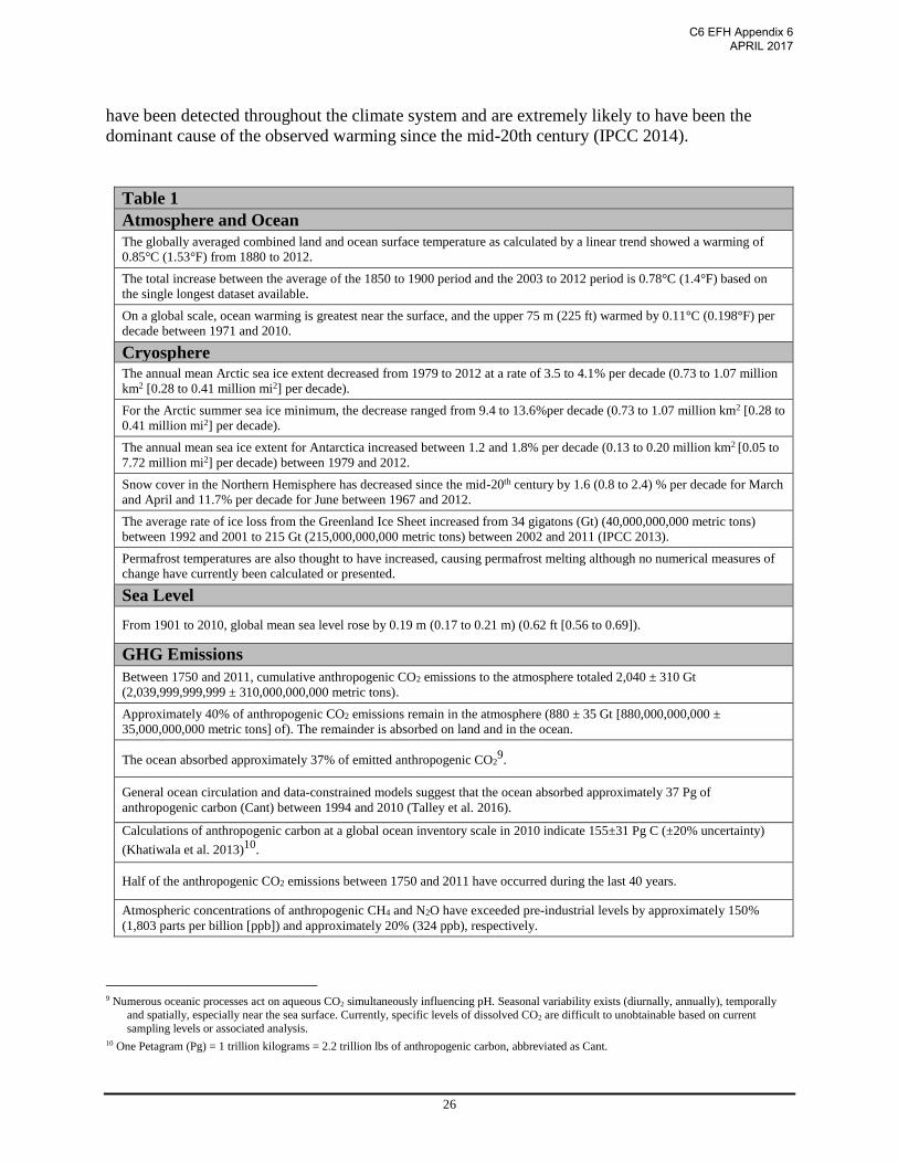
Table 1

Atmosphere and Ocean

The globally averaged combined land and ocean surface temperature as calculated by a linear trend showed a warming of

0.85°C (1.53°F) from 1880 to 2012.

The total increase between the average of the 1850 to 1900 period and the 2003 to 2012 period is 0.78°C (1.4°F) based on

the single longest dataset available.

On a global scale, ocean warming is greatest near the surface, and the upper 75 m (225 ft) warmed by 0.11°C (0.198°F) per

decade between 1971 and 2010.

Cryosphere The annual mean Arctic sea ice extent decreased from 1979 to 2012 at a rate of 3.5 to 4.1% per decade (0.73 to 1.07 million

km2 [0.28 to 0.41 million mi2] per decade).

For the Arctic summer sea ice minimum, the decrease ranged from 9.4 to 13.6%per decade (0.73 to 1.07 million km2 [0.28 to

0.41 million mi2] per decade).

The annual mean sea ice extent for Antarctica increased between 1.2 and 1.8% per decade (0.13 to 0.20 million km2 [0.05 to

7.72 million mi2] per decade) between 1979 and 2012.

Snow cover in the Northern Hemisphere has decreased since the mid-20th century by 1.6 (0.8 to 2.4) % per decade for March

and April and 11.7% per decade for June between 1967 and 2012.

The average rate of ice loss from the Greenland Ice Sheet increased from 34 gigatons (Gt) (40,000,000,000 metric tons)

between 1992 and 2001 to 215 Gt (215,000,000,000 metric tons) between 2002 and 2011 (IPCC 2013).

Permafrost temperatures are also thought to have increased, causing permafrost melting although no numerical measures of

change have currently been calculated or presented.

Sea Level

From 1901 to 2010, global mean sea level rose by 0.19 m (0.17 to 0.21 m) (0.62 ft [0.56 to 0.69]).

GHG Emissions

Between 1750 and 2011, cumulative anthropogenic CO2 emissions to the atmosphere totaled 2,040 ± 310 Gt

(2,039,999,999,999 ± 310,000,000,000 metric tons).

Approximately 40% of anthropogenic CO2 emissions remain in the atmosphere (880 ± 35 Gt [880,000,000,000 ±

35,000,000,000 metric tons] of). The remainder is absorbed on land and in the ocean.

The ocean absorbed approximately 37% of emitted anthropogenic CO29.

General ocean circulation and data-constrained models suggest that the ocean absorbed approximately 37 Pg of

anthropogenic carbon (Cant) between 1994 and 2010 (Talley et al. 2016).

Calculations of anthropogenic carbon at a global ocean inventory scale in 2010 indicate 155±31 Pg C (±20% uncertainty)

(Khatiwala et al. 2013)10.

Half of the anthropogenic CO2 emissions between 1750 and 2011 have occurred during the last 40 years.

Atmospheric concentrations of anthropogenic CH4 and N2O have exceeded pre-industrial levels by approximately 150%

(1,803 parts per billion [ppb]) and approximately 20% (324 ppb), respectively.

9 Numerous oceanic processes act on aqueous CO2 simultaneously influencing pH. Seasonal variability exists (diurnally, annually), temporally

and spatially, especially near the sea surface. Currently, specific levels of dissolved CO2 are difficult to unobtainable based on current

sampling levels or associated analysis. 10 One Petagram (Pg) = 1 trillion kilograms = 2.2 trillion lbs of anthropogenic carbon, abbreviated as Cant.


27

Large Marine Ecosystem

Alaska naturally experiences a wide range of extreme weather and climate events that affect

ecosystem processes, human society, and supporting infrastructure. Recent evidence and

analyses indicate that Alaska has warmed twice as fast as the rest of the U.S. and experienced

significant changes in weather patterns. The state-wide average annual air temperature has risen

by 1.7°C (3°F) and average winter temperature by 3.3°C (6°F) with substantial year-to-year and

regional variability (Stewart et al. 2013).

Gulf of Alaska

Climate and ocean conditions in the North Pacific Ocean and Gulf of Alaska (GOA) have shifted

between cool and warm periods or regimes, particularly over the past 90 years. For example, a

“regime shift” occurred around 1976 and 1977, when ocean conditions shifted from a cold to a

warm phase that has been correlated with the Pacific Decadal Oscillation (PDO). The majority of

fisheries and oceanic scientists, and managers recognize this shift and have acknowledged that a

complex suite of atmospheric and oceanic variables influenced this change.11 In general, this

shift in the GOA is thought to favor the production of some pelagic (upper water column) species

in warm periods and some demersal (bottom dwelling) species in cold periods. An example is

total Alaska salmon production (harvest), which generally inhabit the upper water column, is

reported to be higher in warm regimes than in cool regimes (Mantua et al. 2009).

Potential mechanisms that led to this regime shift are presented in two proposed hypotheses. The

first hypothesis suggests changes in the eastern North Pacific Ocean are driven largely by

atmospheric pressure, related winds and water movements, and subsequent surface layer mixing

and benthic upwelling all influence plankton production (Brodeur et al. 1996, Mantua et al. 1997,

Francis et al. 1998). A second hypothesis suggests that strong recruitment of forage fish and

invertebrates depends on emergence of their larvae at the same time plankton prey are available,

commonly referred to as the “Match-Mismatch” hypothesis (Cushing 1990, Anderson and Piatt

1999). Collectively, climate-forced changes influenced atmospheric and ocean conditions

altering the timing (phenology) and presence of larval and juvenile fish populations to available

plankton prey and possibly exposed larval and juvenile fish populations to increased predation. A

subsequent, weaker climate pulse occurred in 1989 but did not return the GOA or Eastern Bering

Sea to pre-1976/1977 conditions (Hare and Mantua 2000). The prevailing reorganization of the

marine ecosystem produced a dramatic decline in forage fish and invertebrate populations, and a

predominance of groundfish which currently persists (Anderson et al. 1997, Anderson and Piatt

1999, Litzow 2006, Clark et al. 2010).

Anomalously warm water conditions currently continue in the GOA as a result of unusually quiet

winter weather conditions, a weak Aleutian low weather system, and abnormally high sea level

pressure off the coast of the Pacific Northwest. The resulting condition, termed the “warm blob,”

first appeared off Alaska’s southern coast during the fall of 2013 and persists as of this review

11 Multiple hypotheses are proposed on interactions and relationships of Pacific Decadal Oscillation (PDO), El Niño Southern Oscillation (ENSO),

Eastern Pacific warming (EPW), and Central Pacific warming (CPW), all of which influence GOA oceanic conditions, trophic dynamics, and

fisheries. However, these details are beyond the current scope of this report.


28

(Bond et al. 2015, Peterson et al. 2016, Yasumiishi and Zador 2016). This warm water mass is

estimated to be nearly 2,000 km wide and 100 m deep (1,243 mi by 300 ft). Water temperatures

between 1°C and 3°C (1.8°F and 5.4°F) are well above the long-term seasonal average (Bond et

al. 2015, Peterson et al. 2016). The mass may be supported by cyclical weather patterns of high

atmospheric pressure that dominates the weather pattern over western North America (Anderson

et al. 2016). There is speculation that this atmospheric and oceanic influence is generated with

corresponding conditions from the western North Pacific (Zador 2014, Kintisch 2015, Peterson

et al. 2015).

The appearance of the warm blob coincided with a variety of unusual biological events, such as

extremely low chlorophyll levels during late winter/spring of 2014, presumably due to

suppressed nutrient transport into the mixed layer. Several fish species common to warmer

southern waters have been sighted in the GOA and British Columbia. Humboldt squid

(Dosidicus gigas) and skipjack tuna (Katsuwonus pelamis) were caught near the mouth of the

Copper River in July of 2015. Ocean sunfish (Mola mola), and the common thresher shark

(Alopias vulpinus) were documented off the coast of Southeast Alaska far north of their typical

range. Pacific pomfret (Brama japonica) and Pacific saury (Cololabis saira) species associated

with subtropical waters were also abundant in this northern region (Gallagher 2014, Medred

2014, Bond et al. 2015, Orsi 2016, Yasumiishi and Zador 2016). Record high numbers of Fraser

River sockeye salmon (Oncorhynchus nerka) were also documented migrating around the

northern side of Vancouver Island versus the traditional southern migration.

Bering Sea

Historically, the Bering Sea has always exhibited some inter-annual variability in air and sea

surface temperature (SST) and sea ice extent. This seasonal variability has remained relatively

consistent at decadal scales and largely dependent on the frequency and magnitude of low

pressure atmospheric systems (Wyllie-Echeverria and Wooster 1998). Recent atmospheric,

oceanic, and fisheries survey data and analyses indicate subtle changes in Arctic and subarctic

weather patterns and ocean conditions. Stabeno et al. (2001) and Grebmeier et al. (2006b)

identified that SSTs in the Bering Sea had warmed 0.23°C (0.41°F) per decade since 1954.

Between 1972 and 1998, this gradual warming trend was also reflected in the southern extent and

spatial distribution of sea ice. Although the later years in this broad time series reflected a

slightly cooler leveling, SSTs never returned to previous historic lows, sea ice extent was never

as far south, and sea ice residence time was shorter (Stabeno et al. 2001).

As Eisner et al. (2014) present, between 2000 and 2010, the Bering Sea experienced different

multi-year climate shifts (Stabeno et al. 2012b) including above average SSTs and very low sea

ice coverage (2000 to 2005) and a single transition year with average SSTs and sea ice extent

(2006) followed by extremely cold years with extensive sea ice (2007 to 2009). In concurrence

with this warming period (2000 to 2005), there was a decline in Bering Sea walleye pollock

(Gadus chalcogrammus) recruitment which led to a 40 percent decline in the total allowable

commercial harvest (Ianelli et al. 2013). Further data analysis strongly suggested that the decline

in pollock recruitment and biomass during the warm years was a direct result of altered trophic

dynamics from the changing ocean conditions (Farley and Trudel 2009, Coyle et al. 2011, Hunt

et al. 2011, Heintz et al. 2013, Eisner et al. 2014). Simply, the decreased sea ice extent and early

sea ice retreat changed ocean conditions and altered the timing of zooplankton blooms, leading


29

to a decrease in the availability of large lipid-rich plankton, which are normally abundant during

late sea ice retreat, and an increase in the availability of small lipid-poor plankton species.

Pollock juveniles (age 0 to 1) had less prey available in both quality and quantity, experienced

lower energy levels, and became susceptible to predation from other species and cannibalism.

Consequently, the decreased prey availability led to reduced pollock recruitment numbers and

reduced harvest levels (Ianelli et al. 2013).

Just as SST and sea ice extent signaled this extended warm pulse, benthic waters in the same

region reflected a simultaneous warm pulse during the same years. Benthic fisheries and

temperature data suggested a similar trend of increasing benthic temperatures (the cold pool)

between 1982 and 2006 (Mueter and Litzow 2008). The cold pool is a recurrent benthic sea

water zone with persistent temperatures of 0°C to 2°C (32°F to 35.6°F). Sea surface ice cover

provides the character for this benthic zone which is formed as stratification isolates the deeper

cold waters from warmer surface water exchanges. The extent of SST, sea ice cover, and the

benthic character of the cold pool are directly correlated. Consequently, the cold pool had

retreated north from its previous southern extent by approximately 230 km (143 mi), and

subsequent shifts occurred in the distribution of some benthic fish species. Of the 40 taxa that

were analyzed, 11 showed a linear response to shifting benthic temperatures and moved into the

slightly warmer benthic zone previously occupied by the cold pool (Mueter and Litzow 2008). A

similar study conducted by Kotwicki and Lauth (2013) assessed the spatio-temporal

displacement of the same populations in multiple directions using data through 2010. Results

also indicated a reduction in the extent of the cold pool and an increase in the ranges of many of

the same benthic taxa. However, this analysis also introduced additional mechanisms, such as

spatial distribution, nutrition, ontogeny, and spawning, into climate-forced change.

These climate-forced changes represented one of the first well documented occurrences where a

multiyear climate-forced change altered trophic dynamics or influenced the range and

distribution, and abundance of some Bering Sea taxa. Although this warming pattern or pulse

was relatively brief (2000 to 2005) and immediately followed by characteristically cold weather

patterns resuming from 2007 through 2012 (Sigler et al. 2011, Stabeno et al. 2012a, Stabeno et

al. 2012b, Kotwicki and Lauth 2013), current indicators suggest a similar warming pattern may

be occurring presently (2014 through 2016) (Farley 2016). If multiyear climate-forced warming

patterns are more numerous and persistent in the future, projections indicate that there is a

potential for changes in the range, distribution, and abundance of fisheries and increased

uncertainty in modeling predictions and stock assessments (Mueter et al. 2011, Hollowed et al.

2013).

Arctic

The Arctic Ocean is the world’s smallest ocean and has limited exchange with other global

oceans as it is surrounded by continental land masses, has relatively shallow shelves, and is often

covered by ice (NPFMC 2009b). Alaska’s Arctic Ocean is divided into two regional adjacent

seas: the Chukchi Sea and the Beaufort Sea. Generally, fisheries productivity in the Chukchi and

Beaufort Seas is considered low due to extreme environmental conditions. The marine

characteristics of both seas are strongly influenced by terrestrial freshwater runoff; 10 percent of


30

worldwide runoff drains into 3 percent of its total oceanic area (NPFMC 2009b)12. Seasonally,

limited sunlight and freezing Arctic conditions promote the formation of sea ice, which directly

limits trophic interactions and the range and distribution of fish populations. Conversely, melting

summer sea ice nourishes primary production as algae and nutrients are re-released, creating a

highly productive and nutrient-rich, estuarine-like nearshore corridor.

The Chukchi and Beaufort seas are driven by different environmental, climate, nearshore, and

terrestrial influences. Each exhibits different degrees of biological productivity and different

EFH attributes. Comparatively, the Chukchi Sea is generally more productive than the Beaufort

Sea as a result of nutrients and plankton flowing north from the Bering Sea (Woodgate and

Aagaard 2005, NPFMC 2009b). There is also significant seasonal freshwater and nutrient

influence from prevailing western ocean currents and the Yukon River discharge (Dittmar and

Kattner 2003, Dittmar 2004, Woodgate and Aagaard 2005, Spencer et al. 2008, Letscher et al.

2013, McClelland et al. 2016). In the Beaufort during the summer, strong west winds may induce

upwelling of cold, nutrient-rich nearshore waters. Benthic organisms move inshore and support

nearshore fish and invertebrate populations. The McKenzie River plume also influences nutrients

and trophic dynamics in nearshore Beaufort Sea fisheries (Dunton et al. 2006, Dunton et al.

2012, von Biela et al. 2013, Bell et al. 2016).

As Rand and Logerwell (2011) discuss, trends in ocean warming and declines in Arctic sea ice

increase the potential for northward migrations of fish and invertebrate species from the Bering

Sea and North Pacific (IASC 2004, Grebmeier et al. 2006a, Grebmeier et al. 2006b, Mueter and

Litzow 2008, Mueter et al. 2009). As previously discussed, changes from Arctic to subarctic

conditions have been observed in the Bering Sea with a shift from benthic to pelagic fish species

(Overland et al. 2004, (Grebmeier et al. 2006a, Grebmeier et al. 2006b). Similar changes have

been documented in Atlantic and North Sea fish communities (Beare et al. 2004, Perry et al.

2005). The effects of recent record-breaking ice recessions in the Arctic on marine fish

communities are unknown because data are limited or nonexistent (Stroeve et al. 2007, Greene et

al. 2008, Stroeve et al. 2008, Boé et al. 2009).

Currently, no federally managed commercial fishery exists in either the Chukchi or Beaufort

Seas. Marine ecosystem processes that support EFH attributes, such as trophic interactions,

primary and secondary production, and fisheries range and distribution have been assessed but

are not entirely understood (Logerwell et al. 2011, Rand and Logerwell 2011). The seasonal

influence of sea ice significantly limits the ability to access waters to achieve fisheries abundance

and productivity data. Based on surveys conducted in 2010, fish comprised only 6 percent of the

total weight even though 34 taxa of fish were identified. Invertebrate species comprised the

remaining 94 percent of the catch. The majority of fish species that were identified were

nearshore forage fish species that are not federally managed (Logerwell et al. 2011, Rand and

Logerwell 2011) .

The impacts and stressors of climate change appear dramatic in Arctic ecosystems when

considering ocean warming, continued loss of sea ice, and potential ocean acidification (ACIA

2005). However, weather conditions and seasonal sea ice still limit access to prolonged marine

12 Some variability exists in the literature on the volume of freshwater discharge into the Arctic ocean and the total continental shelf area. For

example, Lammers et al. (2001) imply that 11 percent of the world’s freshwater discharge enters 1 percent of the world’s volume in seawater. The Arctic ocean contains 25 percent of the world’s continental shelf.


31

studies or commercial fisheries operations. Generally, little is known of marine fish distribution,

abundance, diversity, or habitat use patterns in the winter (NPFMC 2009a, b). Climate change

and uncertainty in resource availability exacerbate the challenges of predicting impacts or fishery

development.

Cumulative Impacts of Climate Change to Marine Fisheries

Seasonal and decadal variability in climate patterns influence the range, distribution and

abundance of marine fish species at some spatial or temporal scale. Scientists have some

understanding of this influence, and subsequently fisheries scientists and managers account for

some degree of variability in establishing sustainable harvest levels. The influence of climate

change on Alaskan fisheries is presented in the previous examples; one from the Pollock fishery

in the Bering Sea and the second in the changing distribution of southern fish species appearing

in the north Pacific. These examples currently represent relatively short lived “pulse” events,

over a couple years. On the other hand, it needs to be recognized that sea surface temperatures

are predicted to increase in frequency and intensity. These persistent “press” events, in terms of

decades, will exacerbate cumulative impacts subsequently decreasing the precision needed to

implement appropriate fisheries management measures. Increasing frequency of rapid change

complicates accurate assessment of the status of stocks and ability to forecast sustainable levels

of harvest. Numerous subject matter experts have presented how increasing frequency and

intensity of climate change will impact fisheries and fishery-dependent communities through a

complex suite of linked processes and responses (Scavia et al. 2002, Harley et al. 2006, Brander

et al. 2010, Hollowed et al. 2013)13.

Impacts on Ecosystem Productivity and Habitat

If atmospheric CO2 levels continue to increase, global physical models project increased sea

temperatures in many regions, changes in locations and magnitudes of wind patterns and ocean

currents, loss of sea ice in Polar Regions, and a rise in the sea level (IPCC 2014). The

accumulation of CO2 in the atmosphere and associated climate changes is expected to increase

ocean acidification and expand oligotrophic gyres (Doney et al. 2012). These physical and

chemical changes are expected to result in shifts in the timing, species composition, and

magnitude of seasonal phytoplankton production (Cochrane et al. 2009, Wang and Overland

2009, Polovina et al. 2011, Doney et al. 2012). Changes in phytoplankton species composition

may include population shifts to smaller sizes that could lengthen food chains and increase

assimilation losses to higher trophic levels (Mora´n et al. 2010, Bode et al. 2011). These

physical, and resulting biological, changes will occur at different spatial and temporal scales

throughout the world’s oceans (Burrows et al. 2011, Gnanadesikan et al. 2011, King et al. 2011).

Changes in temperature, nutrient supply, mixing, light availability, pH, oxygen, and salinity are

expected to affect the ecological functions and, consequently, the sustainable harvests available

from the ocean’s biological communities (Cochrane et al. 2009, Brander 2010, Denman et al.

2011, Doney et al. 2012). Exposure of marine organisms to ocean acidification and oxygen

depletion will vary regionally, and other anthropogenic impacts (e. g., eutrophication) may also

exacerbate impacts. The vulnerability of the species and a species response under these changes

13 Hollowed et al. (2013), represents a consensus of international subject matter experts in climate change and marine fisheries.

This publication addressing potential cumulative impacts of climate change across large marine ecosystems and associated

fisheries represent potential similar impacts to Alaska’s marine ecosystem processes, fisheries and communities, and was

adopted for use in this report, with permission.


32

varies considerably (Whitney et al. 2007, Feely et al. 2008, Vaquer-Sunyer and Duarte 2008,

Levin et al. 2009, Ries et al. 2009, Rabalais et al. 2010).

Regional differences in primary production are also anticipated. In mid-latitudes the mixed layer

depth (MLD) is projected to shoal, which could decrease nutrient supply and ultimately primary

production. For example, an inter-comparison study of 11 models projected that the ocean’s

MLD will change (decrease or shoal) in most regions of the North Pacific during the 21st century

as the result of increased stratification resulting from warming and/or freshening of the ocean

surface and changes in the winds (Jang et al. 2011). A study using four Earth System Models

(ESMs) found a similar pattern in the North Atlantic (Steinacher et al. 2010). Capotondi et al.

(2012) also provide a global treatment of stratification changes. Primary production in mid-

latitudes is expected to be reduced by this MLD shoaling through decreased nutrient supply

(Hashioka and Yamanaka 2007, Barange and Perry 2009). However, production may increase in

higher latitudes especially in seasonally ice covered areas through increased light levels and a

longer period of production and changes in the ice-edge bloom (Perrette et al. 2011). Increased

stratification caused by sea surface freshening and/or warming is also a main driver of ocean

deoxygenation through decreased ventilation (Whitney et al. 2007). Rykaczewski and Dunne

(2010) hypothesized that decreased ventilation in upwelling zones may increase production due

to increased residence times (the period where producers are retained in the high production

zone) and nutrient remineralization; however, we note that these benefits could be offset by

reduced nutrient supply. There remain important uncertainties regarding how physical and

biological processes are incorporated into projection models (e.g. temperature response; Taucher

and Oschlies 2011) and how these models represent coastal and shelf sea areas (e.g. Holt et al.

2012).

The responses of secondary production to climate change are not clear, partially because the data

available for zooplankton are more limited and the mechanisms linking secondary production to

ocean conditions are complex. In the North Atlantic, the total abundance of zooplankton changed

with sea surface temperature (SST) change (Richardson and Schoeman 2004). However, this

overall pattern masks important trends in the zooplankton community where the abundance of

both herbivorous and carnivorous copepods increased with phytoplankton abundance but the

abundance of neither group was directly correlated with SST. Several authors have recognized

that the phenology of zooplankton may also be affected by a changing climate in both the

Atlantic and Pacific (Chiba et al. 2004, Edwards and Richardson 2004, Mackas et al. 2007).

Although climate change results in an earlier onset of production cycles, the actual timing and

changes in the magnitude of production varied in direction and was influenced by different

mechanisms among regions (Richardson, 2008). Our limited understanding of the trophodynamic

linkages between phytoplankton and zooplankton adds considerable uncertainty to projections of

the responses of these groups to global change (Ito et al. 2010).

Impacts on marine fish and shellfish

Climate-driven changes in the environment may affect the physiology, phenology, and behavior

of marine fish and shellfish at any life-history stage, and any of these effects may drive

population level changes in distribution and abundance (Loeng and Drinkwater 2007, Drinkwater

et al. 2010, Jørgensen et al. 2012). Fish and shellfish will be exposed to a complex mix of

changing abiotic (e.g. temperature, salinity, MLD, oxygen, acidification) and biotic (shifting

distribution, species composition, and abundance of predators and prey) conditions making it


33

more difficult to predict their responses. Climate-driven changes in ocean temperatures may shift

population distributions causing predator–prey overlap, increasing predation mortality or

potentially altering post-recruit abundance. Climate influenced change in the distribution of

predator-prey relationships, for example the decrease in one species and the subsequent increase

in an associated predator species, will lead to increasing levels of uncertainty in stock

assessments (Mueter et al. 2013, Spencer et al. 2016).

Many climate-related changes have already been observed (Perry et al. 2005, Mueter and Litzow,

2008, Barange and Perry 2009, Nye et al. 2009). Kingsolver (2009) identified three types of

potential responses of species to climate change: distribution changes in space and time,

productivity changes, and adaptation. The extent of population-level changes may be mediated

by the capacity for individual species/populations to adapt to changes in important abiotic and

biotic factors through changes in the phenology of important life-history events (e.g. migration,

spawning), or through changes in organismal physiology (e.g. thermal reaction norms of key

traits such as growth; Portner 2010) and/or through acclimation (Donelson et al. 2011).

Mismatches may occur when shifts in the environment lack consistent patterns or out-pace the

species ability to adapt or acclimate to change (Burrows et al. 2011, Duarte et al. 2012).

Changes in life cycle dynamics will occur in concert with climate-induced expansion,

contraction, and/or shifts in the quality and quantity of suitable habitat, and different life stages

may be affected differently by changes in habitat characteristics (Petitgas et al. 2013). Moreover,

in some regions, changes in temperature will be accompanied by changes in other abiotic factors.

For example, expected regional changes in precipitation could lead to decreases or increases in

local salinities which will have major impacts on distributions and productivities of fish species

in coastal and estuarine areas. Thus, perhaps future thermal conditions may be suitable for new

immigrant species, but shifts in salinities could make these waters uninhabitable, illustrating the

challenges of projecting future trends in species richness of fish communities.

Hollowed et. al. (2013) present a summary of 30 recently published studies (2002-2013)

providing evidence that climate change is influencing the spatial distribution of marine fish

species. Although there are many accounts of temperate species moving to higher latitudes,

presumably in response to warming (Beare et al. 2004, Perry et al. 2005), there is less evidence

of contraction of ranges of boreal species (Genner et al. 2004, Rijnsdorp et al. 2010). The

distributional changes may be the result of either active migration of living marine resources to

higher latitudes or from differential productivity of local populations in lower and higher

latitudes (Petitgas et al. 2012), and usually the causal factors are poorly documented. The

sensitivity of fish and shellfish stocks to climate change may differ depending on whether the

stock is at the leading, trailing or center of the species range (Beaugrand and Kirby, 2010). In

some cases, latitudinal shifts will exacerbate mismatches due to concurrent changes in the light

cycle and the duration of the growing season (Kristiansen et al. 2011, Shoji et al. 2011).

The aforementioned impact of climate change on MLD and ocean chemistry has been shown to

exacerbate vertical habitat compression for some highly migratory species of billfish and tunas in

the tropical Northeast Atlantic Ocean. Initial work demonstrated how the near-surface density of

many high-oxygen demand species of pelagic fish was much higher in the eastern than in the

western tropical Atlantic (Prince et al. 2010). Eastern boundary current conditions off the west

coast of Africa create an oxygen minimum zone that is much closer to the surface than in the

western tropical Atlantic. The habitat compression has led to higher vulnerabilities to surface


34

fishing gear and artificially high indications of abundance. Stramma et al. (2011) reported that a

decrease in the upper ocean layer dissolved oxygen occurred in the tropical Northeast Atlantic.

This change equated to an annual habitat loss of approximately 15% over the period 1960–2010.

Climate change is expected to further expand the Atlantic oxygen minimum zone due to

increased ocean temperatures and decreased oxygen levels, potentially threatening the

sustainability of the pelagic fisheries and their associated ecosystems.

Climate change may also influence recruitment success, which will impact population

productivity (e.g. Hare et al. 2010, Mueter et al. 2011). The resilience to shifts in production may

vary by region. In many regions, fish and shellfish have evolved within systems impacted by

intermittent (1–2 years) or longer term events that occur on decadal or multidecadal timescales

(Baumgartner et al. 1992, Hare and Mantua 2000, Greene and Pershing 2007, Di Lorenzo et al.,

2008, Hatun et al. 2009, Overland et al. 2010, Alheit et al. 2012). These events will probably

continue to occur in the future. It is unclear whether species and communities that have

experienced such variability in the past will be better adapted to future climate change. In some

well-documented cases, climate variability is thought to provide opportunities for dominance

switching and ecosystem reorganization (Skud 1982, Southward et al. 1988, Anderson and Piatt

1999, Rice 2001, Stenseth et al. 2002, Chavez et al., 2003). Climate change may interrupt or

accelerate these cycles of dominance switching with unknown implications for both dominant

and subordinate species within each phase of a cycle.

The responses of individual marine species to climate change will vary by species and region

resulting in a broad spectrum of potential shifts in geographic ranges, vertical distributions,

phenologies, recruitment, growth, and survival. Thus, alterations in both the structure (i.e.

assembly and connectivity) and function (i.e. productivity) of biological communities are

expected. Large-scale losses and shifts in community structure, associated with disease, have

been observed elsewhere and are thought to be unprecedented since the Holocene and Late

Pleistocene (Aronson et al. 1998; Greenstein et al. 1998). Physical and chemical changes, and

alterations in temperature influence carbonate saturation, and other climate-driven conditions

increase vulnerability to disease in some fish and shellfish populations (Lafferty 2004, Harvell

2009, Burge 2014). Community responses are the most uncertain types of ecosystem responses

to climate change because they involve more players (all the species in the community and the

habitats that are used), their interactions, and direct as well as indirect effects of climate drivers

(Stock et al. 2011), as well as the spatial and temporal complexity of responses (Burrows et al.

2011; Gnanadesikan et al. 2011). However, there is some evidence that community assemblages

tend to move in concert based on retrospective studies of species spatial patterns and species

richness (Hofstede et al. 2010, Lucey and Nye 2010).

Impacts on Fisheries and Fishery Dependent Communities

Fisheries and fishery-dependent communities have been subjected to fluctuations in fish stocks,

extreme weather events, and natural changes in climate and sea-level throughout history. Coastal

livelihoods have depended on the capacity to cope with such changes through the alteration of

fishing practices or switching to alternative livelihoods (Allison et al. 2009, Perry et al. 2011).

The capacity for human communities to respond to changes in the species composition,

abundance, and availability of marine resources vary regionally (Daw et al. 2009). Climate

change effects on fish and fisheries will occur within the context of existing and future human

activities and pressures, as well as the combined effects of multiple stressors and natural agents


35

of change acting directly and through feedback pathways (Ruckelshaus et al. 2013). In coastal

ecosystems, pollution, eutrophication, species invasions, shoreline development, and fishing

generally play more important roles as drivers of change than on the high seas.

It will be difficult to tease out the additional effect of climate change from other anthropogenic

activities (such as fishing; Rogers et al. 2011). In some cases, where time-series are long enough

or can be re-constructed, the relative importance of different forces can be quantified (e.g. Eero

et al. 2011). Hare et al. (2010) examined the combined effects of fishing and climate in a

modelling context and found that fishing likely remains the dominant pressure, especially at the

historically high fishing levels. Other researchers found that it was difficult to separate the

influence of anthropogenic climate change from decadal environmental variability and fishing

even with a century of data (Engelhard et al. 2011, Hofstede and Rijnsdorp 2011), whereas

others note that fisheries can amplify or moderate climate signals (Ottersen et al. 2006). Some

promising alternative approaches to address these issues include: comparative studies,

experiments, and opportunistic studies of major natural or anthropogenic events (Megrey et al.

2009, Murawski et al. 2010). Ainsworth et al. (2011) used five Ecopath with Ecosim models to

simulate changes in primary production, species range shifts, zooplankton community size

structure in response to ocean acidification, and/or ocean deoxygenation. Fishing pressure was

also included as an additional perturbation to the modelled food web. Their study revealed that

responses to the cumulative effects of climate change and fishing may result in different patterns

than would have been predicted based on individual climate effects, indicating possible

interactions.

The degree to which fisheries are managed sustainably varies globally (Worm and Branch,

2012). In many regions, efforts are underway to prevent overfishing, rebuild overfished stocks,

and implement an ecosystem approach to management (Murawski, 2007). In the future, the

detrimental effects of climate change on fish stocks may, to some extent, be buffered in stocks

that have a large and productive spawning-stock biomass, a less truncated age structure, and

sustainable exploitation rates (Costello et al. 2012). For example, cod have remained abundant

with wide size/age structure in some areas (i.e. Øresund) where exploitation has been low,

although temperatures have increased and while abundance has declined and age structure has

narrowed in neighboring areas [North Sea, Baltic Sea (Lindegren et al. 2010)].

Natural scientists and economists are partnering to develop the projections of how fishers may

respond to changes in fish distribution and abundance (Haynie and Pfeiffer 2012). It is unclear

how complex management systems involving measures such as catch shares, bycatch limits,

mixed species catch or effort limits, and spatial or temporal closures will perform as the species

composition, distribution, and abundance of fish species change (Criddle 2012). An equally

challenging issue is predicting how different nations will utilize the broad range of ecosystem

services that marine ecosystems provide (Halpern et al. 2012). Multispecies management

strategy evaluations can be used to evaluate the expected performance of management

frameworks with respect to balancing these complex issues (Plaga´nyi et al. 2011). However,

selecting the functional form of responses necessary to predict how fishers will respond to

changes in marine resources will continue to be challenging.

The fish stocks, fisheries, and marine ecosystems that coastal communities depend on can be

described as components of coupled marine social-ecological systems (Perry et al. 2011). This is

a particularly useful representation when considering the policy goals of preserving the health of


36

the marine ecosystem while maintaining the supply of desirable goods and services that support

human livelihoods. The representation requires specifying the scale of the system, its properties

(e.g. resilience, biodiversity, productivity, social capital), how it is, or can be, governed, and

what structures and information are required for such governance. Management and governance

approaches may need to be adapted to the available scientific and management capacity

(including financial and social resources). While strengthening capacity may put extra demands

on management agencies and stakeholders, it also brings with it greater sustainable benefits

through reduced uncertainty (Cochrane et al. 2009 and 2011). Anthropogenic climate change is

an increasingly influential driver of change in such social-ecological systems, added to an

already complex set of natural and anthropogenic drivers. The impacts of climate drivers are

manifested on time-scales that are generally longer than most other anthropogenic drivers to

which these social-ecological systems routinely respond.

There is growing recognition of the need for much stronger integration of social and ecological

sciences in developing adaptation options for industries and coastal communities (Allison et al.

2009, Daw et al. 2009, Miller et al. 2010, Gutierrez et al. 2011). In this context, there may be

much to learn from the dynamics of small-scale fisheries in coastal communities. Institutions

such as the FAO and Worldfish are active in working on climate change adaptation in such

systems. Adaptation and mitigation depend on actions and behavioral choices by the

communities who are exploiting the marine resources (whether for fisheries, tourism, or other

goods and services), as well as a supportive wider governance environment to address threats

and constraints to adaptation and mitigation that are outside the control of local communities.

Resource users and communities, within the context of an integrated ecosystem approach, must

have the capacity and the will to adapt and mitigate. Viable adaptation and mitigation actions

require the identification of vulnerabilities at levels from the household to macroeconomic ability

to diversify livelihoods for income and the availability of environmentally sustainable

livelihoods and development options. For example, “co-benefits” of both adaptation and

mitigation can arise from biodiversity conservation, and protection and restoration of mangroves,

and other coastal vegetation (Ruckelshaus et al. 2013). Coastal resources governance can be

encouraged to develop community-based disaster risk management and to integrate climate

change issues into the local and national socio-economic development planning. These actions

may help to prepare communities for climate change impacts on livelihoods that depend on

marine resources.

Implications for Future Security of the Food Supply

The expansion of the world’s human population and current levels of hunger in many parts of the

world have raised concerns over the security of the food supply in the future (OECD 2008,

Godfray et al. 2010 and 2011). Fish currently provide essential nutrition to 4 billion people and

at least 50% of the animal protein consumed by 400 million people (Laurenti 2007, FAO 2012),

currently contributing 17 kg of fish per capita and year. Most of the expected increase in the

human population to 2050 occurs in regions where fish provide most of the non-grain dietary

protein (UN-DESA 2009, UN-WHO 2002). The extent to which marine fisheries will be able to

provide fish for the world’s population in the future will depend on climate driven changes to the

productivity of the world’s oceans and the performance of fisheries management systems (Bell et

al. 2009, Worm et al. 2009, Costello et al. 2012). Several scientists have used outputs from IPCC

global climate models to explore quantitatively or qualitatively the potential consequences of


37

climate change on fish and fisheries production and the implications in terms of food security

targets (e.g. Merino et al. 2012). These studies concluded that even with improved management,

there is only a modest scope for increases in sustainable global yields for capture fisheries (Rice

and Garcia 2011, Brander 2012). However, innovation in both large-scale and small-scale

aquaculture may support a continued increase in production from marine and freshwater systems

(FAO, 2008a, b, OECD 2008, Garcia and Rosenberg 2009, Rice and Garcia 2011, Merino et al.,

2012). At present, global aquaculture production is very unevenly distributed with Asia

accounting for 89% of world production (FAO, 2012). In addition, the effects of climate change

on prospects for fisheries and aquaculture show strong regional differences (Merino et al. 2012).

Substantial political and financial investment in aquaculture will be required in suitable climatic

and environmental regions if it is to provide greater contributions to food security and meet the

growing demand for fish and seafood products. Growing international trade in fish products and

fishing fleet capacities is accentuating regional differences in potential fish consumption

(OECD-FAO 2009, Kim 2010).

Hence, in addition to direct impacts of climate change on fish populations and communities, and

thus food production, there can be indirect impacts through changes to the availability of

alternative sources of protein, to the conditions suitable for intensive culture of fish and shellfish,

and even to the complex interactions of climate on the global trade in food.

Potential Adverse Impacts

It is widely recognized that climate change has the potential to influence ecosystem processes at

regional scales. Examples presented here (Section 2.1.2) of recent observations in the GOA,

Bering Sea, and Arctic exemplify climate induced changes in Alaska’s fisheries. Alaska naturally

experiences a wide range of extreme weather and climate conditions that influence fisheries. The

added influence of climate induced change further complicates our understanding of the natural

variability in these extreme conditions. Currently, it is very difficult to accurately predict the

level of impact to EFH or FMP species.

Despite many of the currently anticipated impacts of climate change, there is no evidence that the

physical oceanic circulation patterns and tides will be altered. Though the severity of an Arctic

winter may decrease, there is no evidence that the length of winter and summer seasons,

specifically the periods of light and darkness will be altered. However, climate change may

influence larger weather patterns and associated seasonal precipitation and snow fall levels.

Some regions may see significant increases in temperatures and water volumes while others

regions may see significant decreases. There is a high level of uncertainty in how future changes

will impact EFH attributes at regional and ecosystem scales.

At the watershed level, throughout Alaska changing seasonal or annual precipitation events may

create more wetlands and wetland complexity. Changes in ground and surface water regimes

may influence instream flows from headwater streams to larger river and estuarine processes.

Precipitation patterns may alter water holding capacity of wetlands and watersheds. Increasing

annual precipitation levels on an already saturated landform may increase flood events and scour

river bottoms. Ice scour in watersheds may damage hyporheic substrates and may prove

detrimental to some anadromous salmon species in their embryonic phase. On the other hand,

warming climate patterns may prove beneficial to many fish species that no longer endure


38

freezing winter conditions. Rising ground and surface water regimes in other regions may

provide increased instream flow or temperatures and prove beneficial to some anadromous

salmon species by minimizing freezing winter conditions under the ice.

In estuarine and nearshore zones, EFH may experience further decreases in the extent and

duration of seasonal ice presence in Arctic and sub-Arctic seas. This may expose entire regions

of Alaska’s coast to continued shoreline erosion. Decreasing sea ice may increase the frequency

and severity of coastal storms and subsequent shoreline erosion. Increased coastal erosion may

alter natural sediment processes and substrate composition, changing trophic dynamics and

further influencing the range and distribution of larval and juvenile fish species in nursery

grounds that represent adults seen later in marine commercial fisheries. As discussed, decreasing

sea ice extent has been shown to impact marine trophic levels and alter abundance and

recruitment of economically valuable marine fish species.

Decreases in sea ice extent allow for increased vessel traffic, and in recent years, the length of

the summer vessel transit season has been longer (Mellgren 2007, Reiss 2008, NPFMC 2009b).

The Arctic Council’s Arctic Marine Shipping Assessment presents an evaluation of impacts due

to increased Arctic shipping activities (Arctic Council 2009, Fretheim et al. 2011). Shipping and

vessel traffic through the Arctic is projected to increase should climate change further reduce the

extent and duration of Arctic sea ice. Expansion of Arctic natural resource development is also

projected; however, that expansion is highly dependent on a multitude of economic influences.

With the exception of northern Norway and northwest Russia, a significant lack of critical

infrastructure limits Arctic marine operations. Extensive gaps in hydrographic, oceanographic,

and meteorological data exist for significant portions of the primary shipping routes, which are

critical for supporting safe navigation. Subsequently, there is an increased potential to introduce

additional anthropogenic stressors, such as the release of oil through accidental or illegal

discharge, ship strikes to marine mammals, increased noise and sonic disruption, and the

introduction of invasive species. Indigenous cultures have expressed concern for the social,

cultural, and environmental impacts of such commercial expansion (ACIA 2005, Arctic Council

2009). Despite potential for increases from climate forced stress in Arctic processes, the winter

season will remain devoid of sun light and remain relatively cold when the suns elevation

declines each winter (Sigler et al. 2011). This in itself may minimize some forms of marine

operations. Additional information on increasing vessel traffic can be found in section 6.4.1.

Continued declines in sea ice may further alter trophic dynamics from primary and secondary

production through apex marine predators. While these impacts may negatively alter one species

range and distribution, it could also prove beneficial to other species increasing their abundance.

Those changes in one species abundance may create additional unseen impacts to other fish

species as a result of predator-prey interactions. Increasing atmospheric temperatures have

already influenced the range, duration and thickness of Arctic sea ice. The continued decline in

the presence of Arctic sea ice may actually accelerate additional decline and may further

influence seasonal weather patterns in Arctic and sub-arctic regions of Alaska.

The continued melting of established tundra permafrost wetlands in the Arctic may increase the

release of greenhouse gases into the atmosphere and may liberate concentrations of terrestrial

carbon, nitrates and phosphates into watersheds and marine systems. These releases may further

exacerbate impacts of climate change in ways we do not currently understand or predict. These

cumulative impacts to freshwater and marine ecosystem processes may be detrimental to some


39

EFH and FMP fish species while having completely beneficial impacts to other species. It is

highly uncertain how the cumulative impacts of so many influences could impact regional

ecosystems.

Climate change may introduce increasing variability in ecosystem processes and species

biodiversity, but it could also stimulate additional development throughout the Arctic. As

permafrost thaws and economic activity in a region expands, the risks associated with

engineering and operations may also increase. Decreasing severity of winter weather patterns

may improve transportation opportunities, infrastructure and shipping logistics, which in turn

may increase opportunities to expand both terrestrial and marine mining (Bankes 2010). A

survey conducted by Jackson (2014) suggests that of the 485 mining industry representatives that

responded to surveys, Alaska ranked in the top 10 of 112 jurisdictions that were favorable and

attractive for future investment.

With increased potential of development comes certain probability of development challenges

associated infrastructure and engineering in the Arctic. In regions where warming or thawing

permafrost have occurred, there is also increased occurrence of compromised foundations and

structural instability of buildings, roads and railways. Thawing permafrost is structurally weak,

resulting in settling that damages infrastructure (Schaefer et al. 2011, Schaefer et al. 2012).

Constructing and maintaining roads, railways, and building structural foundations on unstable,

thawing permafrost is poorly understood (Ljunggren and Rocha 2011). The integrity of

manmade structures and pipelines built on thawing permafrost could collapse and increase the

likelihood of accidents like oil and chemical spills.

Recommended Conservation Measures

NOAA is responsible for applying an “ecosystem approach to sustainable fisheries

management14”. Federally managed species designated with fisheries management plans

(FMPs), must be managed in a manner that ensures long term sustainable yields. To this goal,

species distribution and abundance data is collected and evaluated; spanning diverse habitat

conditions and for various life history stages. Stock assessments are conducted to determine

future sustainable harvest. Many of these indicators are presented in the Ecosystem

Considerations Chapter found within the annual Stock Assessment and Fisheries Evaluation

(SAFE) report (Zador 2015) (NPFMC 2015a, b, e). The report summarizes recent analysis and

highlights trends and changing conditions, that may inadvertently guide future fisheries data

collection and analysis.

As identified in several papers cited in this section, the expanding influence of climate change

has the potential to introduce increasing variability in accurately predicting the condition of

fisheries in the future. Should these currently identified trends continue or intensify, they

14

NOAA Fisheries is responsible for the stewardship of the nation's living marine resources, habitats, interactions

and ecosystems, under mandates derived from numerous key statutes including the: 1) Magnuson-Stevens

Fishery Conservation and Management Act, 2) Endangered Species Act, 3) Marine Mammal Protection Act, 4)

National Aquaculture Act, and 5) National Environmental Protection Act. An ecosystem approach was adopted

to address all these mandates simultaneously and also consider cumulative effects of management decisions and

human influences (Executive Order 13547 of July 19th 2010; Ocean Research Advisory Panel 2013).


40

threaten sustainable management of marine fisheries. Adding to the difficulty, the best indicators

of climate change and ocean acidification (e.g., temperature, salinity, oxygen, and carbonate

chemistry) are not currently collected at spatial and temporal scales that accurately represent

Alaska’s LME’s and subsequent fisheries. A common theme from subject matter experts in

marine fisheries under the influence of climate change, is the need to identify and address key

“data and information gaps” (Griffis et al. 2008, Osgood 2008, NOAA Ocean Acidification

Steering Committee 2010). Without robust and targeted data collection and analysis of key

ecosystem indicators, accurate assessment of change in the fisheries can be increasingly difficult

to identify and consider in management actions.

It is widely recognized that human influences to ecosystem processes in freshwater systems

influence downstream marine estuaries, and nearshore and coastal zones. These potential impacts

are likely further exacerbated by the prevailing influence of climate change. A growing body of

literature identifies many post project marine monitoring programs are chronically under

sampled and limited historical time-series do not provide statistically defensible analysis of

change, or provide the ability to implement adaptive EFH management measures (Bernhardt et

al. 2005 and 2007, Palmer and Febria 2010). Our ability to measure and discern between climate

changes and anthropogenic impacts becomes more possible with targeted data collection and

analysis of marine systems over longer periods.

Functional ecosystem processes (headwater streams through marine systems) provide water

quality and support species biodiversity, abundance and sustainable fisheries. Ecosystem

variables can be measured and monitored to assess marine conditions, such as the physical,

chemical, or biological components of habitats or the presence, abundance, or distribution of

these habitats. Long term measuring and monitoring of marine habitats and their associated

species should be employed to discern between project impacts and climate change.

General Recommendations

• Conduct pre-project, systematic sampling of a projects impacted region to establish a

baseline to discern between climate driven change or project driven impacts.

• Baseline data collection and post-project monitoring efforts should be commensurate

with the project size, level of effect, and expected project life. A longer timeframe may

be needed should the project affect habitats that are less resilient to recover.

• Select habitat attributes that represent physical, chemical, and biological components,

including the presence, absence, abundance, or distribution of EFH species over time.

• Mitigation measures and reasonable alternatives should consider impacts to EFH with

attention to any long-term influences from climate change.

• Projects that will have decadal-scale effects should consult with or brief NMFS and the

NPFMC for interpretation as to whether or not the activity will adversely affect any

federally managed fishery resource.


41

• Projects should include design alternatives to account for the potential of changing

weather patterns, water levels, increased storm activity (buffering techniques), and

exposure to higher energy environments.

• Action agencies should hold combined meetings with local and regional biological

resource managers and communities to detail climate change uncertainties, include

communities and their resources at risk.


42

Wetlands and Woodlands

Introduction – Current Condition

Whether hydrologically confined or connected to surface and groundwater aquifers, wetland and

woodland complexes are extensive throughout Alaska. The ecosystem processes and functions

provided by these biomes are integral components of water quality, the condition of watersheds

and ultimately support fisheries sustainability. Wetlands typically occur in topographic settings

where surface water collects or groundwater discharges, making the area wet for extended

periods of time (Tiner 1996). Wetlands also exist within and between aquatic and woodland

habitats and typically are influenced by both habitats (Welsch et al. 1995). Wetland and

woodland complexes can be characterized as hydrologically connected or confined

(disconnected) to other ground or surface waters (Naiman and Bilby 1998, Northcote and

Hartman 2004, Furniss et al. 2010). Connected watersheds (open waters in riparian areas and

floodplains) have both bidirectional and unidirectional hydrologic exchanges with riverine

systems. Bidirectional flows (i.e., from wetlands or woodlands to streams/rivers and vice versa)

occur through the lateral movement of surface water and groundwater between the channel and

riparian/floodplain areas. In contrast, unidirectional flows (i.e., from wetlands to rivers/streams

but not vice versa) occur in up-gradient areas (e.g., hillslopes and nearby uplands) outside the

floodplains. Confined wetlands (e.g., isolated wetlands in basins, broad flats, or slopes) have the

potential for only unidirectional hydrologic flows from wetlands to the river network through

precipitation or flooding events but have no groundwater connection or influence (EPA 2015).

Confined wetlands are influenced by climate and geography, and occur across various

hydrologic gradients; from wetlands having permanent connections with perennial channels to

isolated wetlands having little to no ground or surface water connections (Tiner et al. 2002, EPA

2015).

Alaska Metrics

Wetlands

Snowmelt and rainfall saturate the Alaskan landscape, forming extensive freshwater wetland

areas ranging from lowlands and depressions to hillsides and slopes (Hall et al. 1994). Alaska's

wetlands occupy approximately 43 percent or 690,000 km2 (266,410 mi2) of the state's 1.7

million km2 (663,267 mi2) surface area (Dahl 1990). The majority of Alaska’s wetlands are in

the interior, Arctic, and western regions of the state. Interior Alaska encompasses 28.7 million

hectares (ha) (71 million acres [ac]), and the Arctic and western regions contain a total of 37.6

million ha (93 million ac) of wetlands. According to the U.S. Fish and Wildlife Service (2013),

only 43 percent of Alaska's wetlands are mapped with 36 percent available digitally via the

internet.

Due to the expansive terrestrial landscape, Alaskan wetland ecosystem types vary considerably

across geographic regions and climatic zones. Treeless expanses of moist and wet tundra

underlain by permafrost occur in most of the Arctic and northwestern portions of Alaska, while

the interior region contains millions of acres of black spruce (Picea marina), muskeg, and


43

floodplain wetlands dominated by deciduous shrubs and emergents. At least two-thirds of

Alaska’s wetlands are comprised of Palustrine scrub/shrub (Hall et al. 1994). Shrub and

herbaceous bogs dominate much of the landscape. Wetlands are also abundant in the valleys and

basins associated with large river systems such as the Yukon, Kuskokwim, Porcupine, Tanana,

and Koyukuk Rivers (Hall et al. 1994).

Predominant freshwater wetland types include bogs, grass wetlands, and sedge wetlands.

Occurring throughout Alaska, bog habitats include shrub-bog and forested-bog types. Shrub-

bogs are characterized by spongy peat deposits, tannic acidic waters, and an overlying vegetative

layer of thick sphagnum moss. Evergreens and shrubs are the most abundant woody plants found

in forested-bog habitats. Alaska’s grass wetland communities are classified as mesic graminoid

herbaceous which are dominated by water-tolerant grass species that occur in clumps or tussocks

and may be intermixed with pure stands of sedges. Sedge wetlands are dominated by tall sedges,

cottonwood grasses, rushes, or bulrushes and are typically inundated with water. These wetlands

occur in very wet areas of floodplains; in the slow-flowing margins of ponds, lakes, streams, and

sloughs; and in depressions of upland areas (Viereck et al. 1992, ADF&G 2006, Walker et al.

2009).

Woodlands

Alaska’s woodlands are extensive; there are approximately 48.6 million ha (120 million ac) of

forestland with >10 percent tree cover in the state. Alaska’s old-growth coastal temperate

rainforest can be subdivided into different habitat types based on the relative mix of species

which, in turn, is a function of soil type and drainage, elevation, and latitude (Viereck et al. 1992,

Gallant et al. 1995). The cooler temperatures, low sun angles, and shorter growing seasons in

high-latitude forests favor dominance by conifers. Old-growth coastal temperate rainforest first

emerges in regions of south central Alaska such Resurrection Bay or in Cook Inlet. However,

this vegetation type dominates Alaska’s coastal zone from Prince William Sound through

Southeast Alaska to the Pacific Northwest. The major coastal temperate rainforests include

western hemlock (Tsuga heterophylla) (46 percent), mixed hemlock/spruce (26 percent), Sitka

spruce (17 percent), cedar (5 percent), and hardwood/deciduous (4 percent) (ADF&G 2006).

Most of this forestland is found in interior Alaska which stretches from the Kenai Peninsula to

the south slope of the Brooks Range and is classified as “boreal forest.” The boreal forest

occupies over 60 percent of the total forest area of Canada and Alaska. About 5.3 million ha (13

million ac) of forest occurs along Alaska’s southeast coast and is classified as coastal temperate

rainforest. Over 95 percent of this coastal temperate rainforest lies within the Tongass and

Chugach National Forests (ADF&G 2006, Albert and Schoen 2007). Boreal forests are

dominated by coniferous trees; species may vary regionally depending on soil conditions and

variations in the microclimate. Broadleaved trees occur in pure stands or are mixed with conifers.

Needleleaf, broadleaf, and mixed forest communities occur in the interior forested lowland and

upland areas across a variety of sites, such as floodplain terraces, streambanks, lake margins, and

highlands; on burned or otherwise disturbed areas; and near timberline. These forests are

dominated by white (P. glauca) and black spruces. Deciduous forests of balsam poplar (Populus

balsamifera), quaking aspens (P. tremuloides), or a mix of these two species develop on

floodplains of meandering rivers and bottomlands (Viereck et al. 1992, Gallant et al. 1995).


44

The Cook Inlet Transition Zone is defined as a region between the interior boreal and coastal

temperate rain forests, generally ranging from south of the Alaska Range surrounding Cook Inlet

and stretching northward into the Susitna River Valley. This zone has the mildest climate in the

boreal region and is generally free from permafrost (ADF&G 2006). Tall scrub communities

dominated by alder and willow form thickets on streambanks, floodplains, and drainage ways.

Coniferous forests include white, black, and Sitka (P. sitchensis) spruces, while deciduous forests

are dominated by quaking aspen (Populus tremuloides), paper birch (Betula papyrifera), and

black cottonwood (P. trichocarpa). Mixed forest types may contain spruce in combination with

any of these other common broadleaf species (Viereck et al. 1992, Gallant et al. 1995).

Alaska’s high latitude Arctic tundra occurs from the crest of the Brooks Range northward to the

Arctic Ocean and is known as the Arctic Slope. The Arctic Slope includes the northern side of

the mountains, the northern foothills, and the flat coastal plain. It is the only true Arctic

biogeographic province in the U.S. The dominant plant species of tundra habitats are sedges, low

and dwarf shrubs, and graminoids interspersed with forbs as well as mat- and cushion-forming

plants and scattered nonvascular bryophytes (ADF&G 2006). Trees are generally unable to

establish in Arctic tundra habitats due to an underlying impermeable permafrost layer

complemented by thin soils (Viereck et al. 1992). Above tree line elevations in the Alaska,

Brooks, and Chugach Mountain Ranges alpine tundra also occurs. Maritime tundra also is

present along the coastal areas of southwestern Alaska and the western Alaska Bering Sea

Islands (ADF&G 2006).

Physical, Biological, and Chemical Processes

Wetlands

Ecosystem functions and bio-chemical processes in Alaska's wetland types vary widely

depending on regional climate patterns, topography, geology, hydrology, and vegetation

(Quinton et al. 2003, King et al. 2012, Walker et al. 2012, Harms et al. 2016). Recent studies

conducted in Alaska indicate wetland processes increase biological productivity supporting EFH

and associated fisheries. These processes regulate water quality and provide refuge to dependent

aquatic species (Wipfli et al. 2007, Whigham et al. 2012). Decomposed plant matter and detritus

form the foundation of nutrient sources and trophic dynamics for many species of freshwater

invertebrates and fish (Fellman et al. 2009, Shaftel et al. 2011, Dekar et al. 2012, King et al.

2012, Walker et al. 2012). Wetlands facilitate natural biochemical processes that facilitate

hydrologic equilibrium throughout watersheds and provide the foundation for several EFH

attributes.

Generally, wetlands regulate surface and groundwater recharge and discharge, maintain water

balance, and in stream flow (Carter 1996, Bullock and Acreman 2003). Many wetlands primarily

serve as discharge areas releasing water to tributaries. Wetlands connected to tributaries provide

temporary storage of water which decreases runoff velocity, reduces flood peaks, and distributes

storm flows over an extended period of time. This natural water level mitigation reduces in

stream erosion and scour of benthic substrates in the stream beds. Wetlands improve water

quality by effectively sequestering, filtering and removing suspended sediments, heavy metals

and pesticides. Through these natural processes wetlands convert anthropogenic constituents into


45

useful and beneficial organic forms. (Carter 1996, Callahan et al. 2015). Wetlands provide

habitats, including breeding and nesting grounds, for a variety of fish and wildlife species.

Woodlands

The ecosystem functions and processes of Alaska's woodland types also vary considerably

depending on regional climate patterns, topography, geology, hydrology, and species of

vegetation (Oakley et al. 1985). Generally, riparian forests are functionally defined as three-

dimensional ecotones of interaction that include both terrestrial and aquatic components,

providing decomposition and recomposition of the existing fauna/flora. These ecotones extend

vertically down into groundwater regimes and above the canopy, and horizontally across

floodplains and the broader terrestrial landscape (Everest and Reeves 2007). Similar to wetlands,

woodlands also provide a variety of biotic functions. Forest canopies regulate water temperature

by providing shade to watersheds. Woodlands provide large volumes of leaf litter fueling

primary and secondary production and aquatic trophic dynamics. Beneficial to freshwater

fisheries, trees deposit large woody debris (LWD) and root wades, creating instream habitat,

promoting lateral channel meander, pools and riffles, and providing organic nutrient (Everest and

Reeves 2007).

Woodland vegetation influences stream water chemistry through processes including direct

chemical uptake and indirect influences such as supplying organic matter to soils and channels,

modifying water movement, and stabilizing soils (Dosskey et al. 2010). Woodlands also play a

critical role in nutrient cycling between terrestrial and aquatic habitats. Nutrient retention,

especially in regulating denitrification by microbial flora/fauna, and organic input (dead plant

material) directly influence the food availability and growth rates of fish in both upstream and

floodplain habitats (ADF&G 2006). Woodland trees also serve as an important food source for

juvenile salmon rearing in watersheds. Aquatic and terrestrial invertebrates that thrive in

woodland watersheds comprise a substantial biomass of organic nutrients (Broadmeadow and

Nisbet 2004, Dekar et al. 2012). Both diversity and density of aquatic invertebrates is higher in

lakes and streams with abundant woodland areas (ADF&G 2006). Trees also influence fish

habitat by providing inputs of LWD, promote channel structure and complexity and maintain

stream bank stability (NRC 2002, Dekar et al. 2012).

Source of Potential Impacts

Upland Activities

Upland activities can impact EFH through both point source and nonpoint source pollution.

Nonpoint source impacts are discussed here. Technically, the term “nonpoint source” means

anything that does not meet the legal definition of point source in Section 502(14) of the Clean

Water Act (CWA); which refers to discernible, confined, and discrete conveyance from which

pollutants are or may be discharged. Land runoff, precipitation, atmospheric deposition, seepage,

and hydrologic modification (generally driven by anthropogenic development), are the major

contributors to nonpoint source pollution (ADEC 2013a). The major sources of nonpoint

pollution discussed in detail in this document include those listed below.


46

▪ Silviculture/Timber Harvest (Section 3.2.2)

▪ Pesticides (Section 3.2.3)

▪ Urban and Suburban Development (Section 3.2.4)

▪ Road Building and Maintenance (Section 3.2.5)

▪ Flood Control/Shoreline Protection (Section 5.2.11)

Nonpoint source pollution is usually lower in intensity than an acute point source event but may

be more damaging to fish habitat in the long term. Deegan and Buchsbaum (2005) place human

impacts to marine habitats into three categories: (1) permanent loss, (2) degradation, and (3)

periodic disturbance. Nonpoint source pollution may be a periodic disturbance that creates a

situation of degradation and leads to permanent loss. It may affect sensitive life stages and

processes, is often difficult to detect, and have impacts that go unnoticed for a long time. When

population impacts are detected, they may not be tied to any one event or source and may be

difficult to correct, clean up, or mitigate.

The impacts of nonpoint source pollution on EFH may not necessarily represent a serious,

widespread threat to all species and life history stages. The severity of the threat of any specific

pollutant to aquatic organisms depends on the pollutant type and concentration and the length of

time a particular species and its life history stages are exposed to the pollutant. For example,

species that spawn in areas that are relatively deep with strong currents and well-mixed water

may not be as susceptible to pollution as species that inhabit shallow, inshore areas near or

within enclosed bays and estuaries. Similarly, species whose egg, larval, and juvenile life history

stages utilize shallow, inshore waters and rivers may be more prone to coastal pollution than

species whose early life history stages develop in offshore, pelagic waters (Baker et al. 2011).

Silviculture/Timber Harvest

Recent revisions to federal and state timber harvest regulations in Alaska and best management

practices (BMPs) have resulted in increased protection of EFH on federal, state, and private

timber lands (USDA 2015a). These revised regulations include forest management practices,

when fully implemented and effective, may prevent or minimize adverse effects to EFH.

However, if these management practices are ineffective or not fully implemented, timber harvest

could have both short- and long-term impacts on EFH throughout many coastal watersheds and

estuaries. Historically, timber harvests in Alaska were not conducted under the current protective

standards, and these past practices may have degraded EFH in some watersheds.


In both small and large watersheds, there are many complex and important interactions between

fish and forests (Northcote and Hartman 2004). If appropriate environmental standards are not

followed, forest conditions after harvest may result in altered or impaired instream habitat

structure and watershed function. However, when implemented modern forestry practices

prevent or minimize most of the potential effects on EFH. Potential impacts to EFH have been

greatly reduced by the adoption of BMPs designed to protect fish and habitat.


47

There are five major categories of silviculture activities that may adversely affect EFH if

appropriate forestry practices are not followed: 1) construction of logging roads, 2) creation of

fish migration barriers, 3) removal of watershed and streamside vegetation, 4) hydrologic

changes and increased sedimentation, and 5) disturbance associated with log transfer facilities

(LTFs) and in-water log storage (Section 5.2.12). Possible effects to EFH include the following

(Trombulak and Frissell 2000, Northcote and Hartman 2004, EPA 2005, Frissell and Shaftel

2014):

▪ Removal of the dominant vegetation and conversion of mature and old-growth upland

and riparian forests to tree stands or forests of early seral stage;

▪ Reduction of soil permeability and increase in the area of impervious surfaces;

▪ Increase in erosion and sedimentation due to surface runoff and mass wasting processes,

which potentially also affect riparian areas;

▪ Impaired fish passages because of inadequate design, construction, and/or maintenance of

stream crossings;

▪ Altered hydrologic regimes resulting in inadequate or excessive surface and stream flows,

increased streambank and streambed erosion, and loss of complex instream habitats;

▪ Changes in benthic macroinvertebrate populations;

▪ Loss of instream and riparian cover resulting in increased water temperatures;

▪ Increase in surface runoff with associated inorganic and organic contaminants (e.g.,

herbicides, fertilizers, heavy metals, dicing salts, and fine sediments) and higher

temperatures;

▪ Alterations in the supply of LWD and sediment which can have negative effects on the

formation and persistence of instream habitat features; and

▪ Excess debris in the form of small pieces of wood and silt which can cover benthic

habitat and reduce dissolved oxygen levels.

Construction of Logging Roads

Improperly engineered, constructed, or maintained logging roads and the use of these roads can

destabilize slopes and increase erosion and sedimentation (as discussed above). Two major types

of erosion may occur: mass wasting and surface erosion. Mass wasting, such as landslides, debris

slides, slumps, earthflows, debris avalanches, and debris flows, can be directly or indirectly

caused or exacerbated by timber harvest and road building on high-hazard soils and unstable

slopes (Spence et al. 1996). Thus, accelerated erosion rates from roads, because of debris slides,

may range from 30 to 300 times the natural rate in forested areas. However, this varies with

terrain in the Pacific Northwest (Sidle et al. 1985). Erosion from roadways is most severe when

construction practices do not include properly located, sized, and installed culverts; proper

ditching; and ditch blocker water bars (Furniss et al. 1991). Contributing up to 90 percent of the

total sediment production, roads are generally considered to be the major source of sediment to

water bodies adjacent to harvested forest lands (EPA 2005). The eroded sediment, such as rill

erosion and channelized flow or sheet erosion or overland flow, delivery to downslope


48

waterways reduces habitat quality and availability for aquatic macroinvertebrates on which

salmon feed and reduces the exchange of oxygenated water in spawning gravels, decreasing the

survival time of salmon eggs and embryos (Murphy 1995). BMPs included in current federal and

state forest practices require the avoidance of hazardous slopes or the development of site-

specific hazard management plans (EPA 2005, USDA 2008).

Creation of Fish Migration Barriers

Stream crossings (bridges and culverts) on forest roads; that are inadequately designed, installed,

or maintained, can alter the existing waterway through changes to the physical habitat structure,

hydrology, and water quality. This can potentially lead to species loss and altered ecosystem

communities. In addition, it can result in full or partial barriers to both upstream and downstream

fish migration, eliminating or reducing access to spawning sites and fragmenting habitat patches

(Daigle 2010, Maitland et al. 2016). For example, in two watersheds in northwestern

Washington, impassable culverts reduced juvenile coho salmon (O. kisutch) rearing capacity by

30 to 58 percent (Roni et al. 2002, Pess et al. 2003). Currently, 36 percent of the stream crossing

structures in the Tongass National Forest meet juvenile fish passage standards for upstream

migration (USDA 2015a). Forest Plan standards stipulate that juvenile fish will have unrestricted

upstream passage within a defined range of stream flows (USDA 2015a). Current fish passage

standards on the Tongass National Forest stipulate that juvenile fish be able to successfully swim

through culverts during approximately 98 percent of the year (USDA 2015a).

Perched and undersized culverts can accelerate stream flows so that these structures become

velocity barriers for migrating fish. However, perched culverts are prohibited under current

BMPs, and all culverts are now subject to sizing requirements designed to allow for the passage

of fish and significant flood events.

Blocked culverts result from undersized designs or inadequate maintenance of removed debris.

When a culvert is blocked, it can result in displacement of the stream from the downstream

channel to the roadway or roadside ditch, resulting in dewatering of the downstream channel and

increased erosion of the roadway. Under modern BMPs, however; culverts must be properly

sized and maintained.

Culverts and bridges deteriorate structurally over time. Failure to replace or remove them at the

end of their useful life may cause partial or total fish passage blockage. Current BMPs require

the removal of culverts upon road closure unless other measures are warranted. Channel incision

can often occur downstream of a culvert and generally moves upstream. An existing culvert can

act as a grade control, halting the upstream progression of a head cut and causing further channel

regrade (Castro 2003); therefore, caution should be used when removing culverts since the

unchecked upstream progression of a head cut can cause further damage to EFH. Additional

information on culverts is available in the Alaska Department of Fish and Game (ADF&G) and

Alaska Department of Transportation and Public Facilities (ADOT&PF) Memorandum of

Agreement for the Design, Permitting, and Construction of Culverts for Fish Passage (ADF&G

and ADOT&PF 2001), NMFS Northwest Region’s Anadromous Salmonid Passage Facility

Design (NMFS 2011), and ADF&G’s Guide to the Procedures and Techniques used to Inventory

and Assess Stream Crossings 2009-2014 (Eisenman and O’Doherty 2014).


49

Removal of Watershed and Streamside Vegetation

Timber harvest activities that remove streamside vegetation increases the amount of solar

radiation reaching the stream and can result in warmer water temperatures, especially in small,

shallow streams of low velocity. In southeastern Alaska, Meehan (1969) found that the

maximum temperatures of logged streams without riparian buffers exceeded that of unlogged

streams by up to 2.3ºC (36.1ºF) but did not reach lethal temperatures. In cold climates, the

removal of riparian vegetation can result in lower water temperatures during winter, increasing

the formation of ice, damaging, and delaying the development of incubating fish eggs and

alevins.

Adverse effects on Pacific salmon from warm-water temperatures include: (1) delayed or

blockage of adult migration; (2) increased adult mortality and reduced spawning success,

including gamete survival during pre-spawning holding; (3) reduced growth of alevins/

juveniles; (4) reduced competitive success relative to other fishes; (5) out-migration from

unsuitable habitats and truncation of spatial distribution; (6) increased disease virulence with

reduced disease resistance; and (7) potentially harmful interactions occurring with other habitat

stressors (Dunham et al. 2001, Materna 2001, McCullough et al. 2001, Sauter et al. 2001, Marine

and Cech 2004). Current BMPs require the retention of riparian buffers for shade which should

limit changes in water temperature and dissolved oxygen.

By removing watershed or streamside vegetation, timber harvest reduces transpiration losses

from the landscape and decreases the absorptive capability of the groundcover. These changes

can result in increased surface runoff during periods of high precipitation and decreased base

flows during dry periods (Myren and Ellis 1984, Heifetz et al. 1986). Reduced soil strength can

result in destabilized slopes and increased sediment and debris input to streams (Swanston 1974).

Sediment deposition in streams can reduce benthic community production (Culp and Davies

1983) with fine sediment causing mortality of incubating salmon eggs and cap sediment causing

the emergence of alevins (Koski 1981, EPA 2005), thus reducing the amount of habitat available

for juvenile salmon (Heifetz et al. 1986). Cumulative sedimentation from logging activities can

significantly reduce the egg-to-fry survival of coho and chum salmon (O. keta) (Cederholm and

Reid 1987). Reductions in the supply of LWD also result when old-growth forests are removed,

thus, causing a loss of habitat complexity which is critical for successful salmonid spawning and

rearing (Bisson et al. 1988, Murphy and Koski 1989). These effects occur when vegetation is

removed within a stream’s watershed but are intensified when streamside vegetation is removed.

Current riparian buffer standards and BMPs are being implemented in most instances (USDA

2008), and long-term effectiveness studies are being conducted to determine if timber harvest has

any effect on habitat condition (Martin and Grotefendt 2001, Martin 2009).

Hydrologic Changes and Increased Sedimentation

According to the Tongass Land Management Plan Revision (USDA 2015c), forest management

activities affect water quality and quantity and the timing of water flows through changes in soil

and watershed conditions. Most watersheds are in a state of dynamic equilibrium where changes

occur naturally because of changes in weather patterns. Because of the overriding influence of

climate and basin resiliency, changes in streamflow and sediment delivery resulting from

management activities (e.g., timber harvest) are difficult to measure.


50

Sediment is water-transported earth material; it may be transported as either a suspended load or

a bedload. A suspended load is carried within the water column, while bedload material moves

(rolls or bounces) along the bottom of the stream or riverbed. Suspended load causes water to

have a turbid or murky appearance. Under natural conditions, the majority of suspended load and

bedload transport occurs during storm runoff events (USDA 2003).

The mass wasting of soil, streams cutting new channels, and bank erosion are the main natural

processes creating sediment. Landslides cause large but temporary increases in suspended and

bedload sediments. Stream and riverbed or bank erosion may contribute to sedimentation over

long periods of time. Steep terrain and large amounts of rainfall make the land sensitive to

natural sediment production and to sediment produced by road construction and timber-

harvesting activities.

Forest management activities that have the greatest potential to affect soil erosion, including

sheet rill, gully, or mass wasting erosion, are associated with timber harvest and include road and

log-landing construction, rock pit development, and some yarding methods. Road construction

increases soil erosion because of the destabilizing effect of cuts, fills, and drainage alteration and

the lack of protective vegetation cover on road surfaces and other disturbed areas. The actual

amount of erosion caused by roads is not known or reliably quantifiable (USDA 2003).

Sediment that settles on or penetrates into the stream bed is of more concern than suspended

sediment and can lead to long-term deleterious changes to fish and invertebrate populations. Soil

mass wasting constitutes the most potentially damaging type of erosion and is thought to be the

major cause of accelerated erosion resulting from silviculture activities. Although mass wasting

has the potential positive effect of providing new sources of woody debris and gravel, it also

negatively affects aquatic habitats by destroying viable eggs via smothering and bed load

overturn and by destroying habitat elements (e.g., pools, riffles, and log discharge) for fish

(USDA 2003). Standards and guides, BMPs, and other relevant mitigation measures are applied

to minimize these potential adverse effects.


The following recommended conservation measures should be viewed as options to prevent and

minimize adverse impacts of silviculture/timber harvest on EFH and to promote the

conservation, enhancement, and proper functioning of EFH. The references listed below apply to

all conservation recommendations.

▪ For all potential adverse impacts to EFH from silviculture/timber harvest, the current

standards and guidelines for the Tongass National Forest in southeast Alaska can be

found at https://fs.usda.gov/Internet/FSE_DOCUMENTS/stelprdb5367422.pdf. This

Forest Plan is currently being amended; the newly proposed plan (USDA 2015c) is

available at http://www.fs.usda.gov/Internet/FSE_DOCUMENTS/fseprd480655.pdf.

▪ The current standards and guidelines for the Chugach National Forest, including soils and

fish, water, and riparian areas, can be found at

http://www.fs.usda.gov/Internet/FSE_DOCUMENTS/fsm8_028736.pdf. This Forest Plan


51

is currently being revised; the newly proposed plan (USDA 2015b) is available at

http://www.fs.usda.gov/Internet/FSE_DOCUMENTS/fseprd486944.pdf.

▪ The Forest Service Region 10 Best Management Practices Policy, Soil and Water

Conservation Handbook, FSH 2509.22 can be found at

http://www.fs.usda.gov/wps/portal/fsinternet/!ut/p/c4/04_SB8K8xLLM9MSSzPy8xBz9C

P0os3gjAwhwtDDw9_AI8zPyhQoY6BdkOyoCAGixyPg!/?ss=1110&navtype=BROWS

EBYSUBJECT&cid=fsbdev2_038796&navid=160000000000000&pnavid=null&positio

n=Not Yet Determined.Html&ttype=detail&pname=Region 10- Land & Resource

Management.

▪ The Alaska Division of Forestry’s booklet on implementing BMPs for timber harvest

operations (ADNR 2011) includes BMP compliance descriptions and guidance for

compliance monitoring and can be found at

http://forestry.alaska.gov/Assets/uploads/DNRPublic/forestry/pdfs/forestpractices/FRPA_

fieldbook_final_5-11_2.pdf.

▪ The State of Alaska Forest Resources & Practices Regulations (ADNR 2013a, ADNR

2013b) can be found at

http://forestry.alaska.gov/Assets/uploads/DNRPublic/forestry/pdfs/forestpractices/PDF_F

orest_Resources_and_Practices_Act_text-May_2013_update.pdf.

▪ The State of Alaska riparian management standards can be found at

http://forestry.alaska.gov/Assets/uploads/DNRPublic/forestry/pdfs/forestpractices/STRE

AMCLASSIFICATIONMATRIX.pdf.

Stream Buffers

Timber operations in watersheds with EFH should adhere to modern forest management

practices and BMPs, including the maintenance of vegetated buffers along all streams to the

extent practicable to reduce sedimentation and supply large wood. In Alaska, buffer width is site-

specific and varies by stream class (Class I, II, III, IV, and Non-streams), stream process groups

(flood plain, glacial outwash, alluvial fan, low gradient contained, moderate gradient/mixed

control, moderate gradient contained, high gradient contained, palustrine, and estuarine), channel

type and stream gradient and is dependent on the use by anadromous and resident fish. Riparian

management standards differ on public and private lands. Riparian buffers required on federal

lands can be found in the Tongass and Chugach National Forests Resource Management Plans

(USDA 2015c, USDA 2015b). Riparian management on the Tongass National Forest is also

performed in accordance with the Tongass Timber Reform Act; which does not allow

commercial harvesting within 30.5 meters (m) (100 ft) on either side (horizontal distance) of

Class I streams and Class II streams that flow directly into a Class I stream. Riparian buffers

required on other lands must comply with the State of Alaska Forest Resources & Practices

Regulations (ADNR 2013a, ADNR 2013b). See the references listed in the previous section for

more details.


52

Estuary and Beach Fringe

For timber operations adjacent to estuaries or beaches, vegetated buffers should be maintained,

as needed, to protect EFH. Estuaries are ecological systems at the mouths of streams where fresh

and salt water mix and where salt marshes and intertidal mudflats are present. The landward

extent of an estuary is the limit of salt-tolerant vegetation (not including the tidally influenced

stream or river channel incised into the forested uplands), and the seaward extent is a stream’s

delta at mean low water. The estuary fringe is an area of approximately 305 m (1,000 ft) slope

distance around all identified estuaries and should be maintained as unmodified forest. The beach

fringe is an area of approximately 305 m (1,000 ft) slope distance inland from mean high tide

around all marine coastlines. The beach fringe should be maintained as mostly undisturbed forest

that contributes to the maintenance of the ecological integrity of the biologically rich tidal and

intertidal zones (USDA 2015c).

Watershed Analysis

A watershed analysis is a procedure for assessing important riparian and aquatic values and

processes in a watershed context. It is designed to:

▪ Help set the stage for project-level planning and decisions,

▪ Strengthen NEPA analyses and decisions, and

▪ Focus interdisciplinary discussions on key watershed resources (USDA 2008).

The scope and intensity of the watershed analysis should be commensurate with the level of risk

associated with the NEPA decision and the information necessary to support that decision.

Watershed analyses require site-specific, field-based site evaluations and include the following

methods: field inventory of all affected stream reaches to verify fish presence, stream classes,

and channel types; consideration of cumulative effects of past, present, and future timber sales

within the watershed; assessment of current condition; and additional analyses. A watershed

analysis should be incorporated into timber and silviculture projects when possible (Nichols et al.

2013).

Forest Roads

The development of forest roads can be a major cause of increased sedimentation in streams, and

road culverts can block or inhibit upstream fish passage. Roads need to be designed to minimize

sediment transport problems and to avoid fish passage problems. Recommended conservation

measures for forest roads include, but are not limited to, those listed below.

▪ Incorporate erosion control and stabilization measures in project plans for stabilizing all

human-caused soil disturbances. Stabilization measures include treating unstable soils

with effective and appropriate erosion control measures to prevent or minimize

sedimentation and erosion of unstable soils.

▪ Improve engineering, construction, and maintenance of logging roads to reduce

landslides. Avoid construction on highly unstable, uplifted marine sediment and on

slopes in excess of the soil’s internal angle of friction. Avoid locating roads and landings


53

on a slope greater than 67 percent, on an unstable slope, or in a slide-prone area. Seed,

mulch, develop terraces, or combine treatments to control erosion after logging road

construction.

▪ Avoid construction of roads across alluvial floodplains, mass wastage areas, and braided

bottom lands.

▪ Seek road locations that avoid fish streams; cross streams only when other locations are

not feasible and fish habitat can be protected. Where roads are located near fish streams,

avoid the introduction of sediment and debris during clearing, construction, and operation

activities. Restrict logging road density or traffic during the wet season and possibly close

logging roads to manage sediment runoff. Excess excavation material must not encroach

upon the stream course; deposit all excess material in a suitable, stabilized upland site.

Leave as much undisturbed ground cover between the road and the stream as feasible.

Require complete end haul of excess excavation where there is the probability of

downhill movement of that material into the stream. To prevent introducing debris into a

stream in sufficient quantity to degrade water quality, fall trees away from all fish-

bearing waters, standing waters, and other surface waters.

▪ Meet fish passage direction at locations where roads cross fish streams. Specify

permissible uses of heavy machinery and the timing of road construction activities.

▪ Design roads so that drainage structures intercept and carry runoff from the hillside and

inside portions of a crowned road surface for forest roads utilizing through-cuts or

partial/full bench road construction.

▪ Install and space drainage structures as necessary to accommodate peak flows or to

ensure adequate drainage of unstable soils. Slope drainage ditches along the roadbed to

the nearest relief culvert. Discharge from road ditches should be cross drained to filter on

natural forest floor rather than flowing directly into streams.

▪ Avoid the introduction or spread of invasive species during road construction,

reconstruction, and maintenance.

Pesticides

Pesticides are a diverse group of chemical substances intended to prevent, destroy, control, repel,

kill, or regulate the growth of undesirable biological organisms in agriculture and a range of non-

agricultural uses (e.g., forestry, irrigation ditches, stagnant water, etc.). They include insecticides,

herbicides, fungicides, nematicides, molluscicides, rodenticides, repellents, fumigants,

disinfectants, wood preservatives, antifoulants, and others. Over 900 different active pesticide

ingredients are currently registered for use in the U.S. and are formulated with a variety of other

inert ingredients that may also be toxic to aquatic life. Legal mandates regulating pesticides

include the CWA and the Federal Insecticide, Fungicide, and Rodenticide Act. Water quality

criteria for the protection of aquatic life have only been developed for a few of the currently used

ingredients (EPA, Office of Pesticide Programs). In Alaska, the Pesticide Control Program is

administered by the Alaska Department of Environmental Conservation’s (ADEC) Division of

Environmental Health (http://www.dec.state.ak.us/EH/pest/index.htm). Nationwide, the most

comprehensive environmental monitoring efforts have been conducted by the U.S. Geological

Survey (USGS) as part of the National Water Quality Assessment Program.


54

While agricultural runoff is a major source of pesticide pollution in the lower 48 states (Ryberg

et al. 2014, Stone et al. 2014), the most common sources of pesticides in Alaska are from other

human activities, such as fire suppression on forested lands, forest site preparation, noxious weed

control, right-of-way (ROW) maintenance (e.g., roads, railroads, power lines), algae control in

lakes and irrigation canals, riparian habitat restoration, and urban and residential pest control

(ADEC 2015a).

Pesticides are frequently detected in freshwater and estuarine systems that provide EFH.

Pesticides can enter the aquatic environment as single chemicals or as complex mixtures. Direct

applications, surface runoff, spray drift, agricultural return flows, and groundwater intrusions are

all examples of transport processes that deliver pesticides to aquatic ecosystems. Habitat

alteration from pesticides is different from more conventional water quality parameters because,

unlike temperature or dissolved oxygen, the presence of pesticides can be difficult to detect due

to limitations in proven methodologies. This monitoring may also be expensive. As analytical

methodologies have improved in recent years, the number of pesticides documented in fish and

their habitats has increased. In addition, pesticides may bioaccumulate in the ecosystem by

retention in sediments and detritus which are ingested by macroinvertebrates which, in turn, are

eaten by larger invertebrates and fish, the process of bio-accumulation and bio-magnification

(Howell et al. 1992).


There are three basic ways that pesticides can adversely affect EFH: (1) a direct, lethal, or

sublethal toxicological impact on the health or performance of exposed fish; (2) an indirect

impairment of aquatic ecosystem structure and function; and (3) a loss of aquatic

macroinvertebrates that are prey for fish and aquatic vegetation which provides physical shelter

for fish.

Fish kills are generally rare when pesticides are used according to their labels. Most effects of

pesticide exposures to fish are sublethal. This is a concern if they impair the physiological or

behavioral performance of individual animals in ways that will decrease their growth or survival,

alter migratory behavior, or reduce reproductive success. In addition to early development and

growth, many pesticides have been shown to impair fish endocrine, immune, nervous, and

reproductive systems (Moore and Waring 2001). Historically, sublethal impacts of pesticides on

fish health were rarely addressed and, therefore, are poorly understood. Over the past few years,

the study of acetylcholinesterase-inhibiting insecticides has shown that sublethal exposures affect

the fitness of exposed salmonids and, ultimately, may result in population-level consequences

(Johnson et al. 2008, Baldwin et al. 2009, NMFS 2009).

Understanding the consequences of sublethal impacts to fish remains a focus of recent and

ongoing NMFS research (Scholz et al. 2000, Sandahl et al. 2005, Laetz et al. 2009). Between

2008 and 2015, NMFS submitted seven biological opinions to the EPA on the registration of 31

active pesticides whose ingredients can have their own toxic properties that may result in adverse

effects on salmon or their prey. Many of these pesticides can produce severe effects on

individuals as well as populations of Pacific salmonids under NMFS jurisdiction

(http://www.nmfs.noaa.gov/pr/consulation/pesticides.htm).


55

The effects of pesticides on ecosystem structure and function can be key factors in determining

the cascading impacts of those chemicals on fish and other aquatic organisms at higher trophic

levels (Preston 2002). These factors include impacts on primary producers (Hoagland et al.

1996), aquatic microorganisms (DeLorenzo et al. 2001), and macroinvertebrates that are prey

species for fish. For example, many pesticides are specifically designed to kill insects. Not

surprisingly, these chemicals are toxic to insects and crustaceans that inhabit river systems and

estuaries. Overall, pesticides will have an adverse impact on fish habitat if they reduce the

productivity of aquatic ecosystems.

Some herbicides are actually toxic to aquatic plants that provide shelter for various fish species.

A loss of aquatic vegetation could damage nursery habitat or other sensitive habitats, such as

eelgrass beds and emergent marshes.



minimize potential adverse impacts of pesticides on EFH and to promote the conservation,

enhancement, and proper functioning of EFH.

▪ Incorporate integrated pest management plans and BMPs as part of the authorization or

permitting process to ensure the reduction of pesticide contamination in EFH (Fulton et

al. 1999). If pesticides must be applied, consider area, terrain, weather, droplet size,

pesticide characteristics, and other conditions to avoid or reduce effects to EFH.

▪ Carefully review labels and ensure that application is consistent with the product’s

directions. Follow local, supplemental instructions such as state-use bulletins, if

available.

▪ Avoid the use of pesticides within 150 m (500 ft; linear) and/or 305 m (1,000 ft; aerial) of

anadromous fish bearing streams.

▪ For forestry vegetation management projects, follow the ADEC measures that establish a

11-m (35-ft) pesticide-free protective area from any surface or marine water body and

require that pesticides not be applied within 61 m (200 ft) of a public water source

(ADEC 2013a).

▪ Consider current and recent meteorological conditions. Rain events may increase

pesticide runoff into adjacent water bodies. Saturated soils may inhibit pesticide

penetration.

▪ Do not apply pesticides when wind speeds exceed 16 kilometers per hour (kph) (10 miles

per hour [mph]).

▪ Begin the application of pesticide products nearest to the aquatic habitat boundary and

proceed away from the aquatic habitat; do not apply pesticides toward a water body.

Urban and Suburban Development

Urban and suburban development is a major (cumulative) threat to EFH (NMFS 1998a, b).

Urban and suburban development and the corresponding infrastructure result in four broad


56

categories of impacts to aquatic ecosystems: hydrological, physical, water quality, and biological

(CWP 2003).


Direct impacts of general urban and suburban development on EFH are discussed below and are

related to the watershed effects of land development, including stormwater runoff. Other

development-related impacts, including dredging (Section 5.4.1), discharge of fill material

(Section 5.4.4), and flood control and shoreline protection (Section 5.4.11), are discussed in later

sections of this document.

Development activities within watersheds and in coastal marine areas can impact EFH during

both long- and short-term timeframes. The Center for Watershed Protection (CWP) conducted a

comprehensive review of the impacts associated with impervious cover and urban development

and found a negative relationship between watershed development and 26 stream quality

indicators (CWP 2003). The primary impacts identified include: (1) the loss of hyporheic zones

(the region beneath and next to streams where surface and groundwater mix) and riparian and

shoreline habitat and vegetation and (2) runoff. Removal of riparian and upland vegetation has

been shown to increase stream water temperatures, reduce supplies of LWD, and reduce sources

of prey and nutrients to the water system. An increase in impervious surfaces in a watershed,

such as the addition of new roads, buildings, bridges, and parking facilities, results in a decreased

infiltration to groundwater and increased runoff volumes. These impacts can adversely affect

water quality and the shape of the hydrograph in downstream water bodies (i.e., estuaries and

coastal waters) (EPA 2007).

The loss of hyporheic zones and riparian and shoreline habitat and vegetation can increase water

temperatures and remove sources of cover. Such impacts can alter the structure of benthic and

fish (i.e., salmon) communities. Shoreline stabilization projects (Section 5.2.5) that alter

reflective wave energy can impede or accelerate natural movements of shoreline substrates,

thereby affecting intertidal and subtidal habitats. The channelization of rivers causes a loss of

floodplain connectivity and a simplification of habitat. The resulting sediment runoff can also

restrict tidal flows and elevations, resulting in losses of important fauna and flora (e.g.,

submerged aquatic vegetation [SAV]).

Runoff from impervious surfaces (e.g., buildings, rooftops, sidewalks, parking lots, roads,

gutters, storm drains, and drainage ditches) is the most widespread source of pollution into the

nation’s waterways (EPA 1995). Runoff from urban development is an emerging threat,

particularly to ecosystems along all coastal margins of the U.S. (McCarthy et al. 2008, Weiss et

al. 2008) since urban and suburban development in the U.S. continues to expand in coastal areas

at a rate approximately four times greater than inland areas. Impacts from urban and suburban

development are generally difficult to control because of the intermittent nature of rainfall and

runoff, the large variety of pollutant source types, and the variable nature of source loadings

(Safavi 1996). Runoff includes pollutants such as construction sediments, oil from vehicles, road

salts, bacteria from failing septic systems, and inorganic and organic contaminants (i.e., heavy

metals). The 2000 National Water Quality Inventory (EPA 2002) reported that runoff from urban

areas is the leading source of impairment in surveyed estuaries and the third largest source of

impairment in surveyed lakes. While our understanding of the individual, cumulative, and


57

synergistic effects of all contaminants on the coastal ecosystem are incomplete, pollution

discharges may cause organisms to be more susceptible to disease; impair reproductive success;

and cause acute, chronic, and sublethal effects in aquatic species (EPA 2005). Urban areas can

have a chronic and insidious pollution potential that one-time events, such as oil spills, do not.

Salmonids and other anadromous fish appear to be particularly impacted by the proportion of

impervious cover in a watershed (CWP 2003). In a study in the Pacific Northwest, coho salmon

were seldom found in watersheds with above 10 or 15 percent of impervious cover (Luchetti and

Feurstenburg 1993). Other studies have shown that impacts to stream quality can be expected

when a watershed exceeds 10 percent impervious cover (CWP 2003). Key stressors in urban

streams, such as higher peak flows, reductions in habitat complexity (e.g., fewer pools, LWD,

and hiding places), and changes in water quality, are believed to change salmon species

composition, favoring cutthroat trout (O. clarkii) populations over the natural coho populations

(May et al. 1997, Livingston et al. 1999).

Stormwater management systems are often built to move water quickly away from roads,

resulting in increased velocities and higher peak volumes of water in streams. Uncontrolled

higher velocities and higher peak flow volumes of urban stormwater have a greater erosive

capacity than stormwater from a forested watershed. Higher velocities and flow volumes erode

streambanks and increase stream sediment loads. In a simulation model comparing an urban

watershed with a forested watershed, Corbett et al. (1997) demonstrated that runoff from an

urban watershed had 5.5 times greater volume and sediment than runoff from a forested

watershed. Additionally, reduced canopy cover can often cause higher stream temperatures.

Literature reviews and ongoing research illustrate the adverse impacts of urban stormwater

discharge and growing communities on fresh water and marine invertebrate, fish, and marine

mammal populations (Beach 2002, Neff 2002, LaLiberte and Ewing 2006, Weiss et al. 2008).

Urban stormwater also discharges nonpoint pollutants to soil and water, leading to their eventual

bioaccumulation in aquatic species. Polycyclic aromatic hydrocarbons (PAHs) are among the

most toxic to aquatic life and can persist for decades (Short 2003). Waterborne PAH levels are

often significantly higher in urbanized than nonurbanized watersheds (Fulton et al. 1993).

Petroleum-based contaminants contain PAHs which can cause acute toxicity to managed species

and their prey at low concentrations when released into the environment through spill,

combustion, and atmospheric deposition; some PAHs are known carcinogens and mutagens

(Neff 1985).

Sublethal effects of fish exposure to many chemical and metal pollutants often associated with

urban stormwater over time may prove more deleterious than concentrations that are

immediately lethal. Subtle sublethal effects on fish may include changes in behavior, feeding

habits, and reproductive success (Murty 1986). Stormwater contaminants have been shown to

negatively alter cellular function and biochemical machinery in many aquatic organisms. These

impacts may lead to increased mortality in fish species via carcinogenesis through oxidized

metabolites, interference with DNA repair mechanisms, and/or initiation of teratogenesis

(prenatal toxicity that causes structural or functional defects in the developing embryo or fetus).

Some stormwater contaminants disrupt neurotoxic and olfactory responses that maintain normal

homing, predator avoidance, and spawning behavior. They can weaken immune system response


58

and inadvertently increase susceptibility and mortality from diseases. These conclusions are well

documented in a variety of fish species (Neff 1985, Muir et al. 1988, Dethloff et al. 1999,

Hansen et al. 1999a, Hansen et al. 1999b, Baldwin et al. 2003, Sandahl et al. 2007).

Failing septic systems and combined sewer overflows are an outgrowth of urban development.

The EPA estimates that 10 to 25 percent of all individual septic systems are failing at any one

time, introducing excrement, detergents, chlorine, and other chemicals into the environment.

Even treated wastewater from urban areas can alter the physiology of intertidal organisms

(Moles and Hale 2003). Sewage discharge is a major source of coastal pollution, contributing 41,

16, 41, and 6 percent of the total pollutant load for nutrients, bacteria, oils, and toxic metals,

respectively (Kennish 1998). Nutrients such as phosphorus concentrations are particularly

indicative of urban stormwater runoff (Holler 1990) and may lead to algal blooms,

eutrophication, loss of biodiversity, and the expansion of invasive species. Sewage wastes may

also contain significant amounts of organic matter that exert a biochemical oxygen demand

(Kennish 1998). Organic contamination contained within urban runoff can also cause

immunosuppression and increased susceptibility to diseases in juvenile salmon (Arkoosh et al.

1998, Arkoosh et al. 2001).



minimize adverse impacts of urban and suburban development on EFH and to promote the

conservation, enhancement, and proper functioning of EFH.

▪ Implement BMPs for sediment control during construction and maintenance operations

(EPA 1993). These BMPs may include: (1) avoiding ground-disturbing activities during

the wet season; (2) minimizing exposure time of disturbed lands; (3) using erosion

prevention and sediment control methods; (4) minimizing the spatial extent of vegetation

disturbance; (5) maintaining buffers of vegetation around wetlands, streams, and drainage

ways; and (6) avoiding building activities in areas with steep slopes and areas prone to

mass wasting events with highly erodible soils. Structural BMPs are also recommended

and may include sediment ponds, sediment traps, vegetated swales, or other facilities

designed to slow water runoff and trap sediment and nutrients.

▪ Avoid using hard engineering structures for shoreline stabilization and channelization

when possible. Use bioengineering approaches (i.e., approaches with principles of

geomorphology, ecology, and hydrology) to protect shorelines and riverbanks. For

example, use native vegetation for soil stabilization. Naturally stable shorelines and river

banks should not be altered.

▪ Encourage comprehensive planning for watershed protection and avoid or minimize

filling and building in coastal and riparian areas affecting EFH. Development sites should

be planned to minimize clearing and grading, cut-and-fill, and new impervious surfaces.

▪ Where feasible, remove obsolete impervious surfaces, such as abandoned parking lots

and buildings, from riparian and shoreline areas and reestablish water regime, wetlands,

and native vegetation.


59

▪ Protect and restore vegetated buffer zones of appropriate width along streams, lakes, and

wetlands that include or influence EFH.

▪ Manage stormwater to replicate the natural hydrologic cycle, maintaining natural

infiltration and runoff rates to the maximum extent practicable.

▪ Where Instream Flows (ISF) are insufficient to maintain the water quality and quantity

needed for EFH, establish conservation guidelines for water use permits and encourage

the purchase or lease of water rights and the use of water to conserve or augment ISFs in

accordance with state and federal water laws.

▪ Use the best available technologies in upgrading wastewater systems to avoid combined

sewer overflow problems and chlorinated sewage discharges into rivers, estuaries, and

the ocean.

▪ Design and install proper wastewater treatment systems away from open waters,

wetlands, and floodplains.

▪ Where vegetated swales are not feasible, install oil/water separators to treat runoff from

impervious surfaces in areas adjacent to marine or anadromous waters. Ensure that

oil/water separators are regularly maintained such that they do not become clogged and

function properly on a continuing basis.

Road Building and Maintenance

Roads and trails have always been part of man’s impact on his environment (Luce and Crowe

2001). Federal, state, and local transportation departments devote huge budgets to the

construction and maintenance of roads. In Alaska, roads play an important part in access and,

thus, are vital to the economy (Conner 2007). The potential impacts to EFH associated with the

building and maintenance of paved and unpaved roads are discussed in the following section.


Current road design construction and management practices are a vast improvement from

previous methods. However, roads still have a negative effect on the biotic integrity of both

terrestrial and aquatic ecosystems (Trombulak and Frissell 2000), and the effects of roads on

aquatic habitat can be profound (Daigle 2010). Potential adverse impacts to aquatic habitats

resulting from the existence of roads in watersheds include: (1) increased surface erosion,

including mass wasting events and deposition of fine sediments; (2) changes in water

temperature; (3) elimination or introduction of migration barriers such as culverts; (4) changes in

streamflow; (5) introduction of invasive species; (6) changes in channel configuration; and (7)

the concentration and introduction of PAHs, heavy metals (e.g., copper, lead, zinc), and other

pollutants.

Road building and maintenance can affect aquatic habitats by increasing rates of natural

disturbances, such as landslides and sedimentation, and even properly designed and constructed

roads can become sources of landslides and sedimentation if they are not maintained. Streams,

wetlands, or other sensitive areas located near roads may experience increased sedimentation

from general road maintenance and use, storms, and snowmelt events. Poorly surfaced or

unpaved roads can substantially increase surface erosion. The rate of erosion is primarily a


60

function of storm intensity, surfacing material, road slope, and traffic levels. This surface erosion

results in an increase in fine sediment deposition (Cederholm and Reid 1987, Bilby et al. 1989,

MacDonald et al. 2001), which has been linked to decreased fry emergence and juvenile

densities, loss of winter carrying capacity, and increased predation of fishes in stream gravels.

Increased fine sediments can reduce benthic production or alter the composition of the benthic

community. For example, embryo-to-emergent fry survival of incubating salmonids is negatively

affected by increases in fine sediments in spawning gravels (Koski 1981, Everest et al. 1987,

Chapman 1988, Scrivener and Brownlee 1989, Young et al. 1991, Weaver and Fraley 1993).

Road crossings also affect benthic communities of stream invertebrates. Additionally, studies

show that populations of noninsect invertebrates tend to increase the farther away they are from a

road (Luce and Crowe 2001).

Beschta et al. (1987) and Hicks et al. (1991) document some of the negative effects of road

construction on fish habitat, including the elevation of stream temperatures beyond the range of

preferred rearing where vegetation has been removed, inhibition of upstream migrations,

increased disease susceptibility, reduced metabolic efficiency, and shifts in species assemblages.

Roads built adjacent to streams can result in changes in water temperature due to increased

sunlight reaching the stream if vegetation is removed and/or altered in composition. Roads can

also degrade aquatic habitat through improperly placed culverts at road-stream crossings that

reduce or eliminate fish passages (Evans and Johnston 1980, Belford and Gould 1989, Clancy

and Reichmuth 1990, Furniss et al. 1991).

Roads have three primary effects on hydrologic processes and, therefore, streamflow. First, they

intercept rainfall directly on the road surface, in road cutbanks, and as subsurface water moving

down the hillslope. Second, they concentrate flow either on the road surfaces or in adjacent

ditches or channels. Third, they divert or reroute water from flow paths that would otherwise be

taken if the road was not present (Furniss et al. 1991). Another possible consequence of road

construction on hydrologic processes is the destabilization of the stream channel by intercepting

groundwater flow and channeling water directly into the stream, thus, increasing the frequency

and volume of floods as well as erosion and other associated natural processes. Erosion is most

severe when poor construction practices are allowed and combined with inadequate attention to

proper road drainage and maintenance practices.

Roads can also serve as vectors for introducing nonnative species to a watershed by creating

suitable habitat for invasive species, planting invasive species along roadsides for erosion

control, and serving as a route for the accidental introduction from vehicular or other traffic

traveling along the road system (Trombulak and Frissell 2000).

Pavement and many paving compounds used in road construction, surfacing, and resurfacing and

especially pavement sealing and repair products contain high levels of PAHs (Grosenheider et al.

2005, Mahler et al. 2005, Barsh et al. 2007, Teaf 2008). The friction between road and tire

surfaces erodes and liberates asphalt, rubber material, and chemical compounds. Further

contributions of automotive fluids, fuel, and brake linings concentrate on or near road surfaces

and eventually reach streams and the ocean (Grosenheider et al. 2005, Simon and Sobieraj 2006,

Weiss et al. 2008). PAHs and heavy metals are toxic to aquatic wildlife, particularly fish and


61

invertebrate populations (Rand 1995, Logan 2007) and accumulate in estuarine, nearshore, and

marine fish and invertebrates (Kennish 1997, Johnson et al. 2002, Kennish 2002).


The following conservation measures should be viewed as options to prevent and minimize

adverse impacts of road building and maintenance to EFH and to promote the conservation,

enhancement, and proper functioning of EFH (EPA 1993).

▪ Roads should be sited to avoid sensitive areas, such as streams, wetlands, and steep

slopes, to the maximum extent possible.

▪ Build bridges rather than culverts for stream crossings when possible. If culverts are to be

used, they should be sized, constructed, and maintained to match the gradient and width

of the stream to accommodate design flood flows, and they should be large enough to

provide for migratory passage of adult and juvenile fishes. If appropriate, use the NMFS

Northwest Region’s Anadromous Salmonid Passage Facility Design (NMFS 2011) or the

culvert guidelines contained in the ADF&G and the ADOT&PF Fish Pass Memorandum

of Agreement (ADF&G and ADOT&PF 2001).

▪ Design bridge abutments to minimize disturbances to stream banks, and place abutments

outside of the floodplain whenever possible.

▪ Specify erosion control measures in road construction plans.

▪ Avoid side casting of road materials on native surfaces and into streams.

▪ Use only native vegetation in stabilization plantings.

▪ Use seasonal restrictions to avoid impacts to habitat during species critical life history

stages (e.g., spawning and egg development periods). Recommended seasonal work

windows are generally specific to regional or watershed-level environmental conditions

and species requirements.

▪ Properly maintain roadway and associated stormwater collection systems.

▪ Limit roadway sanding and the use of deicing chemicals during the winter to minimize

sedimentation and the introduction of contaminants into nearby aquatic habitats. Snow-

melt disposal areas should be silt-fenced and include a collection basin. Roads should be

swept after break up to reduce sediment loading in streams and wetlands.

▪ Plan development sites to minimize clearing and grading and cut-and-fill activities.

▪ Protect existing riparian buffer zones, and wherever practicable, establish new riparian

buffer zones of appropriate width on all permanent and ephemeral streams that include or

influence EFH. Establish buffers wide enough to support shading, LWD input, leaf litter

inputs, sediment and nutrient control, and bank stabilization functions.


62

Headwaters, Streams, Rivers and Lakes


Streams, rivers, and lakes are all essential components of complex aquatic ecosystems. The

majority of Alaska’s water resources are generally pristine due to Alaska’s size, remoteness, and

sparse population. It has the fewest impaired water bodies and the greatest number of unimpaired

water bodies in the country (ADEC 2013b, 2015b). Alaska’s vast watersheds are influenced by

complex geomorphology, regional climate and seasonal weather patterns, and terrestrial

vegetation at enormous spatial and temporal scales. Flowing surface waters directed by these

interactions are also supported by three-dimensional subsurface groundwater regimes.

Groundwater regimes support surface waters providing the foundation for habitat complexity,

ISF, biochemical processes, ecosystem function, and abundant fisheries. According to

Sophocleous (2002), surface and groundwater ecosystems are viewed as linked components of a

hydrological continuum. These hydrologic processes provide the foundation for EFH, associated

biogeochemical processes and sustainable fisheries.

In Alaska, landscape and associated vegetation and hydrologic processes are generally

characterized within eight ecoregion descriptions: Arctic tundra in the north, intermontane and

boreal predominant regions in the southcentral region, Bering coastal tundra and taiga, Aleutian

Island meadows, two other distinct mountain transition zones in the Southcentral region, and the

temperate coastal rainforests of the GOA and Southeast Alaska (Nowacki et al. 2001). Within

these terrestrial complexes, a multitude of watershed interactions afford an infinite range of

variations in stream, river, and lake habitats, all of which provide some measure of ecosystem

process or function to EFH associated with anadromous Pacific salmon, the only anadromous

species recognized within FMPs in Alaska. However, although anadromous salmon maybe found

within all these regional descriptions, the species is not well established in the Arctic tundra

ecoregion north of the Brooks Range.

Alaskan Metrics

Alaska includes 44,659 km2 (17,243 mi2) of inland waterways which consist of 12,000 rivers;

thousands of streams and creeks; over three million lakes greater than 2 ha (5 ac); and an

estimated 100,000 glaciers (Glass 1996, ADF&G 2006, NMFS 2015). Approximately three-

fourths of all freshwater resources in Alaska are stored as glacial ice covering about 5 percent of

the state (ADF&G 2006). Alpine glaciers and ice fields, glacial and clearwater rivers and streams

connect many interior water sheds to Alaska's marine estuarine ecosystem (ADF&G 2006). Over

18,000 Alaskan lakes, rivers, or streams are identified as important habitat for anadromous fish.

Southeastern Alaska contains over 5,200 anadromous salmon streams totaling 40,000 kilometer

(km) (24,855 miles [mi]) in length (Halupka et al. 2000). Over 20,000 water bodies used by

anadromous fish have not yet been catalogued or documented in the Anadromous Fish Catalogue

(Anadromous Fish Act [16.05.087(a)]).

Alaska has approximately 563,270 km (350,000 mi) of primary rivers; however the majority of

secondary and smaller headwaters streams have not been mapped (ADF&G 2016). There remain


Impacts to EFH from


63

thousands of miles of headwater streams and EFH that play an important role in emerging and

rearing salmon that have not been surveyed. For example, fisheries surveys recently conducted

by the Southwest Salmon Habitat Partnership, in areas not previously surveyed (Nushagak and

Kvichak River drainages) documented salmon in the majority of headwater streams (Woody and

O’Neal 2010). Of the 168 km (104.3 mi) of headwater streams surveyed, anadromous salmon

were present and documented in 74 percent of head water tributaries. These data support the

hypothesis that nearly every stream in many headwaters with less than 10 percent gradient may

contain rearing salmon species in some life history stage (7 out of 10 streams).

Alaska’s regional watersheds extend from the interior of the state to the Arctic, northwest, and

southern coasts (NMFS 2015). Thousands of rivers and streams enter the GOA from southcentral

to southeastern Alaska, while numerous rivers and streams enter the Bering Sea from western

Alaska and the Alaskan Peninsula. The Yukon River, the longest river in Alaska and the third

longest in the U.S. (Brabets et al. 2000), drains a watershed of over 855,000 km2 (330,117 mi2)

and flows for 3,187 km (1,980 mi) from its headwaters in Canada to the Bering Sea (NMFS

2015). Other large salmon rivers include the Kuskokwim, Stikine, and Copper (Augerot 2005,

ADF&G 2006). The Arctic region is crossed by many northward flowing streams, the largest of

which is the Colville River. This region also contains continuous permafrost, tundra, and

numerous small lakes and ponds (NMFS 2015). Lake Iliamna is Alaska's largest lake with a

volume of 115 km3 (15,968 ft3) encompassing an area of approximately 2,590 km2 (1,000 mi2).

Other large lakes include Clark, Becharof, Naknek, Ugashik, Teshekpuk, Tustumena, Kenai, and

Wood-Tikchik (Augerot 2005, ADF&G 2006).

Alaska's Harding Icefield (777 km2 [300 mi2]), located in the Kenai Peninsula, is the largest in

North America and one of only four remaining icefields in the U.S. Thirty-five of Alaska's

glaciers stem from the Harding Icefield. These glaciers feed and influence nearly all major

riverine systems in Alaska and provide the headwaters to some of the state's largest rivers,

including the Copper, Susitna, and Tanana (ADF&G 2006). Alaska’s freshwater ecosystems

range from the temperate coastal rainforest of the southeast region with maritime climate and

dense riparian vegetation, to the boreal forest of interior Alaska with continental climate and

modest riparian vegetation, and the Arctic tundra of the North Slope with sparse riparian

vegetation (ADF&G 2006).

Physical, Biological, and Chemical Processes

The MSA defines EFH as waters and substrates necessary for fish. EFH not only includes visible

surface water and hard substrate but also habitat attributes and ecosystem processes that provide

water quality, quantity, and nutrient resources essential for survival. For anadromous Pacific

salmon, these waterways provide migratory corridors for both outbound fry and inbound adults,

water quality and quantity over spawning and rearing substrates, protection from freezing winter

conditions as embryos in hyporheic gravel substrates (wet substrates beneath and adjacent to

streams) and nutrient availability during spring emergence and rearing (Scheuerell et al. 2007).

Salmon require cool waters in sufficient quantities to allow for migration and successful

spawning. Relevant geomorphic stream characteristics include channel width, depth and slope,

substrate composition, and pool and riffle sequences. Organic inputs come from canopy leaf

litters and riparian grasses that provide nutrient subsidies. LWD provides shelter, nutrient as well

as promotes lateral channel meander and geomorphic complexity (Scheuerell et al. 2007).


Impacts to EFH from


64

Salmon themselves inadvertently provide nutrient subsidies to watersheds, numerous aquatic and

terrestrial species of flora and fauna, as well as their own progeny. All these biochemical and

geomorphic influences are the ecosystem processes within watersheds that directly influence the

sustainability of salmon populations at numerous life history stages (Boulton et al. 1998, Gende

et al. 2004).

Hyporheic Zone

The hyporheic zone is the interactive ecotone between surface water and groundwater beneath

and alongside rivers and streams (Stanford and Ward 1988, 1993, Brunke and Gonser 1997,

Boulton et al. 1998). It is the gravel substrate where adult salmon deposit eggs and the salmon

embryos develop over the winter. The condition of that substrate and the water moving through

that substrate plays an integral role in embryo development and over winter survival. Three

major types of hyporheic zones have been characterized: wetted channel, parafluvial, and

floodplain scale (Naiman et al. 2000). Interactions within these hydrologic regimes is regionally

based on geology and riverine topography and is often temporal in response to ISFs and seasonal

influences (Winter et al. 1998, Naiman et al. 2000, Sophocleous 2002, Malcolm et al. 2004,

Youngson et al. 2004). The relative contribution of groundwater and surface water to this zone

also varies spatially according to local channel morphology, riparian-stream linkages, and

hydrology. The hyporheic zone influences various watershed ecosystem processes such as

nutrient cycling, vital gaseous exchange, thermal regimes, and even pollutant buffering (Dahm et

al. 1998, O'Keefe and Edwards 2002, Pinay et al. 2002, Battin et al. 2003, Hancock et al. 2005,

Mulholland and Webster 2010).

Depending on the region, watershed, species, or even individual run, salmon eggs and embryos

can be deposited throughout summer and fall months (Schindler et al. 2010). The embryos reside

there until the following spring when they emerge as fry. The hyporheic zone subsequently

supports salmon egg and embryo survival and development through Alaska’s often harsh winters

under freezing conditions (Cunjak and Power 1986, Cunjak 1988, 1996). In Japan, Urabe et al.

(2014) reported that channel morphology via hyporheic flow was a significant determinant in

maintaining population diversity in chum salmon. Salmon spawning activity is usually observed

in gravel substrate with favorable hydraulic properties water gradients and associated

temperature (Power et al. 1999, Geist 2000, Geist et al. 2002, Garland et al. 2003, Schindler et al.

2003, Malcolm et al. 2005, Smith 2005, Huusko et al. 2007).

Headwater Streams

The watershed network can be partitioned into headwater and network systems based on

hydrologic (e.g., precipitation, heat dynamics), geomorphic (e.g., channel reach type, woody

debris), and biological (e.g., organic matter, energy input) process characteristics. These systems

are important sources of sediments, water, nutrients and organic matter for downstream reaches

(Gomi et al. 2002). Four topographic units compose headwater streams: hillslopes (divergent or

straight contour lines, typically no channelized flow), zero-order basins (an unchannelized

hollow with convergent contour lines), transitional channels (temporary or ephemeral channels

emerging from zero-order basins), and first- (upper-most, unbranched channels with perennial or

sustained intermittent flows) and second- (headwaters) stream channels. The complex interaction

of geomorphic and hydrologic processes affects the biological process at various temporal/spatial


Impacts to EFH from


65

scales. The frequency, intensity, and duration of these spatio-temporal scales are important

factors altering the responses and recovery time of riparian vegetation, channel morphology, and

biological communities (Gomi et al. 2002, Freeman et al. 2007).

Headwater streams are abundant and unique aquatic systems that amongst several other attributes

provide habitat complexity, increased prey availability and simultaneous refuge from predation

(Meyer et al. 2007, Whigham et al. 2012). In Alaska, headwater streams are abundant and can be

an important spawning and rearing habitat for juvenile salmonids (Woody and O’Neal 2010,

Copeland et al. 2014). Unlike higher-order stream reaches that receive large volumes of Marine

Derived Nutrient (MDN)15 from salmon carcasses, food webs in headwater reaches are more

reliant on terrestrial subsidies from invertebrates, riparian areas, and instream nutrients (Piccolo

and Wipfli 2002, Wipfli and Gregovich 2002, Wipfli et al. 2007, Dekar et al. 2012, Shaftel et al.

2012, Walker et al. 2012).

Not all Pacific salmon emerge from substrate and emigrate to the sea. Depending on the region,

watershed, species, habitat conditions, and forage opportunities some salmon species, such as

coho and chinook (O. tshawytscha), disperse into small and non-natal streams to take advantage

of rearing and prey opportunities (Bradford et al. 2001, Ebersole et al. 2006, Daum and Flannery

2011, Copeland et al. 2014). Armstrong et al. (2013) recently documented the freshwater phase

juvenile coho salmon moving considerable distances (350 to 1,300 m [1,148 to 4,265 ft]), up and

down stream, daily between warmer and colder water habitats to take advantage of abundant

prey opportunities. Freshwater phase coho exhibiting these feeding migrations had accelerated

their metabolism and digestion, grew faster, and were better prepared for their marine phase.

Levings and Lauzier (1991) identified juvenile chinook salmon using the main stem river to over

winter. Suitable overwinter habitat is also provided to rearing juvenile salmonid as a result of

hyporheic water processes (e.g., groundwater influence, high levels of dissolved oxygen, low-

flow velocities, instream cover LWD, and even anchor ice) (Heifetz et al. 1986, Cunjak 1996,

Reynolds 1997, Mouw 2004, Roussel et al. 2004, Smith 2005, Huusko et al. 2007, Brown et al.

2011, Huusko et al. 2013).

Organic Matter

Organic matter, particularly Dissolved Organic Matter (DOM), and decomposition are important

sources of nutrients for primary production in freshwater ecosystems. Organic matter is

incorporated into stream ecosystems through autotrophic (macrophytes, periphyton,

phytoplankton) and heterotrophic (protozoans, bacteria, macroinvertebrates, aquatic vertebrates)

pathways. Heterotrophic organisms derive energy from DOM, fine and coarse particular organic

matter. These organic inputs usually come from outside the aquatic ecosystem; naturally falling

into waters or forced during storm events, rain fall, periods of spring flooding and snowmelt. The

majority of these sources arrive in the form of needles and leaf litter, grasses and LWD (Vannote

et al. 1980, Bisson and Bilby 1998). Nutrient subsides are also delivered by adult salmon in

anadromous watersheds (see Marine-Derived Nutrients section below). These organic matter

15

The terms Marine Derived Nutrients (MDN) and Salmon Derived Nutrients (MDN) are used synonymously

throughout the current literature depending on the source, discipline or topic. For simplicity, MDN will be used

throughout this report to signify nutrient derived from any life stage of salmon.


Impacts to EFH from


66

sources provide the foundation for primary and secondary production in watersheds. Energy

flows out of net production through shredding, grazing and decomposition of Particulate Organic

Matter (POM) and gradual excretion of DOM. Of these, the main energy flow from producers is

through direct grazing of living tissues and detritus from external sources (Murphy 1998).

Primary production in Alaskan riverine ecosystems is predominantly by benthic algae found

within a complex assemblage of algae, bacteria, fungi, and periphyton (biofilm) (Verspoor et al.

2010). This energy dynamic changes predictably in response to trends in geomorphology and

fluvial processes (Vannote et al. 1980). Export and retention of organic matter into a stream

channel largely determine the contribution of aquatic primary producers to a stream ecosystem.

Both organic matter and nutrients undergo a cycling process called spiraling (Murphy 1998),

which occurs where nutrients are assimilated by living organisms; returned to the stream by

decomposition, respiration, or excretion; and eventually reincorporated farther downstream

(Bisson and Bilby 1998). Streams with short spirals have high retention capacity and efficiently

utilize organic matter and nutrients (Murphy 1998).

In diverse stream environments, macroinvertebrates have an important influence on nutrient

cycles, primary production, decomposition, and translocation of materials. Benthic invertebrates

graze periphyton from mineral and organic substrates; reduce decomposing vascular plant tissue;

feed directly on living vascular macrophytes, decomposing wood, FPOM, and animal tissue

acting as sieves to remove particulate matter from suspension (Mulholland 1992, Wallace and

Jackson 1996). The linkages between flow parameters, resource availability, respiratory/thermal

requirements, and biotic interactions (e.g., competition and predation) influence the structure and

function of these diverse benthic stream ecosystems. Secondary production within these stream

ecosystems includes a combination of features such as abundance, biomass, growth,

reproduction, survivorship, and generation time (Wallace and Jackson 1996). Estimated

production of macroinvertebrate prey and predators in first and second-order low-gradient

streams indicated that invertebrate predators represented 25 to 35 percent of macroinvertebrate

production (Wallace and Jackson 1996, Piccolo and Wipfli 2002, Wipfli and Gregovich 2002,

Wipfli et al. 2007, Wipfli and Baxter 2010).

Tundra and grassland areas have similar physical, chemical, and biological linkages. The

Alaskan tundra is a cold-climate landscape that has vegetation but is devoid of trees (ADF&G

2006), while dry grassland communities occur across boreal regions of Alaska on dry, south-

facing slopes or well-drained lowland sites (Viereck et al. 1992). The overall annual productivity

of these freshwater ecosystems generally consists of low nutrient input levels, low temperatures,

prolonged periods of ice presence, and short growing seasons. Spring-fed streams with stable

environments exhibit a greater diversity in primary producers. Tundra streams tend to be

ephemeral and low in pH and nutrients with corresponding low productivity. Medium-sized

rivers that drain lakes typically have moderate to high levels of productivity and associated

diversity in invertebrate fauna (Wrona et al. 2005).

Marine-Derived Nutrients

Pacific salmon accumulate up to 99 percent of carbon, nitrogen, and phosphorous (among other

nutrients) in their body mass during their ocean phase growth. The salmon spawning migrations

transport large volumes of these MDN back into watersheds. These nutrients cross traditional


Impacts to EFH from


67

ecosystem boundaries, providing nutrient subsidies to other aquatic species (invertebrates and

fish) and terrestrial species (e.g., bears, wolves, and passerine birds) and fertilize a variety of

riparian vegetation (Willson and Halupka 1995, Cederholm et al. 1999, Gende et al. 2002,

Naiman et al. 2002, Hilderbrand et al. 2004, Quinn 2005, Rüegg 2011). MDN increase stream

and river productivity both immediately after spawning and during the following spring. Studies

indicate that these nutrient subsidies introduced during the summer and fall of one year persist in

hyporheic substrates through the following year, providing nutrient sources to resident fish and

invertebrate populations and inadvertently increasing prey abundance for emerging salmon fry

the following spring (Bilby et al. 1998, Hilderbrand et al. 1999, O'Keefe and Edwards 2002,

Hocking et al. 2009, Rinella et al. 2013).

This process influences food webs through bottom-up effects of increased primary and secondary

production (Schindler et al. 2003, Verspoor et al. 2010, Verspoor et al. 2011) or when consumers

switch their diets to salmon (Gende et al. 2001, Scheuerell et al. 2007, Swain and Reynolds

2015). Salmon also liberate and export nutrient from streams through spawning activities (Moore

et al. 2007). Salmon disturb stream beds during nest digging, thereby suspending nutrient-laden

sediments into the water column (Moore 2006). Salmon smolts also transfer nutrients during

their migration to the ocean (Moore and Schindler 2004, Scheuerell et al. 2005). Salmon are net

importers of nutrients to stream and riparian habitats by evidence of nutrient export (Janetski et

al. 2009, Holtgrieve and Schindler 2011). The assimilation of MDN into riparian ecosystems via

these pathways (e.g., hyporheic flowpaths, epilithon layer) varies over time and among different

areas (Mitchell and Lamberti 2005, Helfield and Naiman 2006, Cak et al. 2008, Albers 2010).

Once in the riparian zone, MDN’s are incorporated into a variety of pools including soil organic

matter, vegetation, microbial biomass, and roots (Ben-David et al. 1998, Bilby et al. 2003, Bartz

and Naiman 2005, Wilkinson et al. 2005, Gende et al. 2007, Fellman et al. 2008). Nutrients not

immediately assimilated into watershed processes are transported downstream from headwater

streams to estuaries and nearshore zones (see Estuaries and Nearshore sections).

Riparian Zones

Rivers, streams, and terrestrial ecosystems (i.e., forested or vegetated hillslopes) are strongly

linked. The riparian zone transitions from aquatic vegetation at the wetted edge to terrestrial

vegetation of the upslope forest. The surrounding riparian vegetation affects stream processes

(e.g., radiation inputs and outputs, supply and storage of organic matter [wood and litter]) and

the structure of stream banks (Richardson et al. 2005). Retention and routing of allochthonous

organic matter (e.g., riparian/lateral input of leaf litter and LWD) are important factors affecting

the biological processes in headwater streams (Gomi et al. 2002). Riparian zones are connected

to lotic systems (e.g., small headwater streams to large braided rivers) via the exchange of

materials and organisms. Aquatic food webs derive energy from both in-stream and terrestrial

sources (Vannote et al. 1980). The basic components of food webs (e.g., nutrients, detritus, and

organisms) cross spatial boundaries (Polis et al. 1997). Terrestrial subsidies (e.g., invertebrates,

coniferous needles, deciduous leaves, and woody materials) act as basal resources for many

aquatic organisms (Gutierrez 2011). For instance, terrestrial invertebrates are an import food

source for salmon in headwater and small streams; they account for 50 percent of the prey

consumed by juvenile salmon (Allan et al. 2003).


Impacts to EFH from


68

Hydrology

The hydrology and geology of freshwater ecosystems influence the physical and chemical

characteristics of rivers and streams. For instance, the quality of surface water and groundwater

is strongly affected by ground strata and bedrock geology (Brabets et al. 2000). Land cover

influences a number of hydrologic factors, such as snow accumulation, soil moisture depletion,

surface runoff, infiltration, and erosion. These factors, in turn, can affect the water quality of a

particular stream or river. The composition of certain types of vegetation may also affect water

quality. In addition, land cover directly influences the permafrost because of the thermal

properties that determine the quantity of heat entering and leaving the underlying ground where

the permafrost occurs (Brabets et al. 2000). Streamflow quantity and variability also have

considerable influence on the quality of surface water. The quantity of water in a stream or river

influences its ability to support aquatic communities, to assimilate or dilute waste discharges,

and to carry suspended sediment and geochemical weathering products (Brabets et al. 2000)

Instream flow dynamics, shoreline and benthic deposition and erosion, and sediment transport in

woodland river and stream ecosystems is largely influenced by the presence of LWD. The

persistence of LWD influences channel dynamics by stabilizing banks and substrate material and

by providing subsequent succession of riparian vegetation cover for terrestrial predators. LWD

also promotes the formation of pool habitats and provides spawning bed integrity and habitat for

aquatic invertebrates, elevating in-stream productivity. LWD groundings often lead to the

formation of downstream islands, bars, and slough habitats in large rivers, whereas in smaller

streams, lakes, and ponds, LWD plays an important role in habitat creation immediately adjacent

to the input point. Decaying terrestrial debris often accumulates near LWD, providing a food

source for aquatic invertebrates (Naiman et al. 2000, Gurnell et al. 2002, ADF&G 2006).

Surface and Groundwater Regimes

Surface water regimes support ISF dynamics which supply the primary medium and energy

source for the movement of water, sediment, organic material, nutrients, and thermal energy

(Ziemer and Lisle 1998). Important hydrologic pathways include subsurface, overland, and

Hortonian overland flows. Subsurface flow accounts for nearly all the water that is delivered to

stream channels from undisturbed forested hillslopes. In channels and floodplains, subsurface

flow is very important to benthic and hyporheic organisms. Surface water flows occur where the

ground strata and soils become fully saturated, consequently forcing subsurface waters to emerge

as flowing surface water regimes. The tendency of water to flow horizontally across land

surfaces when rainfall has exceeded infiltration and storage capacity is Hortonian overland flow.

Increased areas of Hortonian overland flow directly contribute to stream peak flows during

storms in headwater channels and have a greater capacity to erode and transport sediment.

In contrast to hillslope runoff, stream flow pertains only to surface flow in the channel (Ziemer

and Lisle 1998). The surface water/groundwater interface is a crucial point for lateral nutrient

fluxes between uplands and aquatic ecosystems and for upstream/downstream (longitudinal)

processes in lotic systems (Sophocleous 2002). Annual winter and spring floods distribute

sediment and organic debris through the stream system, scour the bed, and remove newly

established vegetation in the active channel. These floods can cause mortality of certain benthic

invertebrates, altering food webs which affect the trophic structure of these communities.


https://en.wikipedia.org/wiki/Fluid_dynamics

https://en.wikipedia.org/wiki/Depression_storage_capacity

Impacts to EFH from


69

Through erosion, scour and deposition, extreme floods can create new surfaces that renew

dynamic processes of both aquatic and riparian ecosystems. Recessional spring and early

summer flows, punctuated by peak flows, control the success of riparian plant seeds to germinate

on stream banks and floodplains. Summer low flows allow the settlement of sediments, clearer

water, and low-energy habitats to expand (Ziemer and Lisle 1998).

Channel Morphology

Stream channels are important avenues of sediment transport that deliver eroded material from

freshwater ecosystems to the ocean. Channels ranging in size from small ephemeral streams to

large rivers exhibit a wide variety of morphologies but share a number of basic processes

(Montgomery and Buffington 1998). Channel morphology is influenced by local, systematic

downstream variations in sediment input from upslope sources (frequency, volume, and size of

sediment supply), the ability of the channel to transport these loads to downslope reaches

(frequency, magnitude, and duration of discharge/valley gradient), and the effects of vegetation

on channel processes (bank strength, in-channel size, rate of delivery/decay, and

orientation/position). Potential channel adjustments to altered discharge and sediment load

include changes in width, depth, velocity, bed slope, roughness, and sediment size (Montgomery

and Buffington 1998). Spatial variability in sediment supply may govern channel morphology in

different portions of a drainage network (Montgomery and Buffington 1998). Positions within a

stream network and differences between the transport capacity to sediment supply ratios allow

segregation of channel reaches into source, transport, and response segments. Source segments

are headwater colluvial channels that act as transport-limited sediment storage sites subject to

intermittent debris flow scour. Transport segments are composed of morphologically resilient,

supply-limited reaches (bedrock, cascade, and step-pool) that rapidly convey increased sediment

inputs. Response segments consist of lower-gradient, more transport-limited reaches (plane-bed,

pool-riffle, and dune-ripple) in which significant morphological adjustments occur in response to

the increased sediment supply. The distribution of these segment types defines watershed-scale

patterns of sensitivity to altered discharge and sediment supply (Montgomery and Buffington

1998).


Mining

Mining within riverine habitats may result in direct and indirect chemical, biological, and

physical impacts to habitats within the mining site and surrounding areas during all stages of

operations. On-site mining activities include exploration, site preparation, mining and milling,

waste management, decommissioning or reclamation, and abandonment (NMFS Starnes and

Gasper 2000, 2005b). Mining and its associated activities from exploration to post-operation

have the potential to cause adverse effects to EFH by reducing or altering fish habitats or

populations in affected watersheds (E&E 2010). The operation of metal, coal, rock quarry, and

gravel pit mining in upland and riverine areas has caused environmental damage in urban,

suburban, and rural areas. Some of the most severe damage, however, occurs in remote areas

where some of the most productive fish habitat is often located (Sengupta 1993). In Alaska,

existing regulations promulgated and enforced by other federal and state agencies are designed to


Impacts to EFH from


70

control and manage these changes to the landscape to prevent and minimize impacts. However,

while environmental regulations may avoid, limit, control, or offset many potential impacts,

mining will, to some degree, always alter landscapes, ground and surface water regimes, and

environmental resources (NRC 1999).

Mineral Mining

Mining and mineral extraction activities take many forms, such as commercial and recreational

suction dredging; placer, open pit, and surface mining; and contour operations. The process for

mineral extraction involves exploration, mine development, mining (extraction), processing, and

reclamation.


The potential adverse effects of mineral mining on fish populations and their habitat are well

documented (Goldstein et al. 1999, Brix et al. 2001, Hansen et al. 2002, Farag et al. 2003) and

depend on the type, extent, and location of the mining activities. Recreational gold mining with

equipment such as pans, motorized or nonmotorized sluice boxes, concentrators, rockerboxes,

and dredges can adversely affect EFH on a local level. Commercial mining is likely to involve

activities on a larger scale, resulting in even greater disturbances (Williamson et al. 1995).

Impacts associated with the extraction of material from within or near a stream or river bed may

include: (1) alteration in channel morphology, hydraulics, lateral migration, and natural channel

meanders; (2) increases in channel incision and bed degradation; (3) disruption in pre-existing

balance of suspended sediment transport and turbidity; (4) direct impacts to fish spawning and

nesting habitats (redds), juveniles, and prey items; (5) simplification of in-channel fluvial

processes and LWD deposition; (6) altered surface and groundwater regimes and hydro-

geomorphic and hyporheic processes; and (7) destruction of the riparian zone during extraction

operations. Loss of stream habitat, in particular, is thought to be the single biggest cause of

declines of anadromous salmonids in general (Nehlsen et al. 1991, Reeves and Sedell 1992). In

addition to the potential loss or alteration of habitat of aquatic waterways, mineral mining effects

may include direct and indirect chemical stressors such as mining-related pollution, acid mine

drainage (AMD), altered temperature regimes, reduction in oxygen concentration, and the release

of toxic materials (e.g., cadmium, copper, zinc) (Johnson et al. 2008, E&E 2010). Many of these

impacts have been previously discussed in this document. The discussion below summarizes the

impacts that have not been previously addressed.

Scientific literature has many examples of spawning substrate selection by salmonid species

being influenced by chemical and physical variables such as instream and inter-substrate flow

(hyporheic zone), dissolved gases, nutrient exchange, and temperature. Mining activities may

disrupt these physical and geochemical systems initiating and promulgating mineral dissolution

or precipitation reactions that can alter pre-mining groundwater quality and chemistry in ways

that may be difficult to predict (Lewis-Russ 1997).

Recent studies suggest that diffuse mining-related pollution in rivers may significantly contribute

to the loading of metals, principally because mine water contribution may be influenced by

altered water tables (Younger 2000). Minerals and metals liberated from rock and soil substrates


Impacts to EFH from


71

interact with atmospheric oxygen and water (Jennings et al. 2000, Younger et al. 2002, Jennings

et al. 2008). The introduction of this metal and mineral rich runoff or AMD into the aquatic

ecosystem can have adverse impacts on the ecology of entire watersheds. Once started, AMD is

difficult to stop or reverse. This acidic drainage can dissolve metals and metalloids, causing them

to leach from the mined rock into the environment potentially in toxic levels. AMD also lowers

pH (increases acidity); salmon populations are adversely impacted by acute and chronic

exposure. Salmon are particularly vulnerable to low pH when undergoing the physiological

changes that occur during smolts’ transition from freshwater to salt water and adult spawners’

transition from salt water to freshwater (Chambers et al. 2012). AMD is known to be toxic to

fish, algae, zooplankton, and aquatic invertebrate populations at the ecosystem, metabolic, and

cellular levels (Buhl and Hamilton 1991, Saiki et al. 1995, West et al. 1995, Barry et al. 2000,

Hansen et al. 2002, Peplow and Edmonds 2005, Levit 2010). For example, the release of

cadmium via AMD can cause salmon mortality, and chronic exposure to cadmium can cause

pronounced sublethal effects such as decreased growth, inhibited reproduction, and population

alterations (Levit 2010). The hyporheic zone is especially vulnerable since this zone supports

salmon spawning and incubating eggs as well as production of aquatic insects and aquatic

vegetation. Groundwater may enter the hyporheic zone in an undiluted condition, leading to

injury and mortality of aquatic organisms (including fish) prior to benefiting from the dilution

effects of the overlying streamflow (Brunke and Gonser 1997, Gandy et al. 2007).

Metal contamination and exposure has been shown to influence simple migratory behavior and

avoidance mechanisms in fish populations (e.g., Goldstein et al. 1999, Hansen et al. 1999a, Brix

et al. 2001, Farag et al. 2003, Sandahl et al. 2004). Numerous studies have shown how exposure

to toxic contaminants in surface waters can impact fish olfaction which is critical for behaviors

such as mating, locating prey, and avoiding predators (see Tierney et al. 2010). Copper

contamination in surface waters is common in watersheds with mining activities. McIntyre et al.

(2012) recently evaluated the effects of copper exposure on juvenile coho salmon predator

avoidance behaviors and found that the exposed juveniles were unresponsive to their

chemosensory environment, unprepared to evade nearby predators, and less likely to survive an

attack sequence. Additional studies indicate that salmonids exposed to sublethal levels of metals

are susceptible to increasing levels of fish pathogens due to stressed immune responses and

metabolisms (Jacobson et al. 2003, Peplow and Edmonds 2005, Spromberg and Meador 2005).

The ability to treat or neutralize AMD is very site specific and often unpredictable. Mine waste

will be exposed to the natural elements of weathering over a long period of time (CSS 2002).

Studies on rivers recovering from metal and mineral contamination concluded that despite efforts

to remediate surface water pollution, community recovery in the hyporheic zone may take longer

than surface macroinvertebrate recovery due to the continued release of metals by reductive

dissolution and exposure to AMD. Depending on the scale of the mining operation and

associated topography and hydrogeomorphic processes, active treatment to neutralize AMD may

need to last in perpetuity to be effective (Kuipers 2000, Jennings et al. 2008).

The creation of waste dumps, tailings impoundments, mine pits, and other facilities that become

permanent physical features of the post-mining landscape can cause fundamental changes in the

physical characteristics of a watershed (O’Hearn 1997). Mining and the placement of spoils in

riparian areas can cause the loss of riparian vegetation and changes in heat exchange, leading to


Impacts to EFH from


72

higher summer temperatures and lower winter stream temperatures (Spence et al. 1996). Bank

instability can also lead to altered width-to-depth ratios which further influence temperature

(Spence et al. 1996). Mining efforts can also bury productive habitats near mine sites. Although

reclamation efforts and mitigation practices may restore topographic land forms to mine sites,

these efforts generally fail to restore natural hydrogeomorphic and aquatic functions and

associated water quantity and quality within measurable time frames (Kilmartin 1989, Mutz

1998). Additionally, commercial operations may involve road building (Section 3.2.5), tailings

disposal, and leaching of extraction chemicals which may affect EFH.

In accessing mineral and ore deposits, many mining methods require withdrawals from

groundwater aquifers. These naturally occurring and often saturated groundwater aquifers sustain

ISFs. Altered water regimes may change instream channel morphologies, stream gradients, and

bank and benthic substrates and disrupt the equilibrium between flow and sediment transport in

tributaries (Johnson et al. 1999, Sophocleous 2002). Often these impacts are seen many miles

upstream and downstream of the actual mine site, thus, impacting EFH and anadromous species

by limiting access to migratory corridors and reducing available spawning and rearing habitat.


The following measures are adapted from recommendations in Spence et al. (1996), NMFS

(2005a), and Washington Department of Fish and Wildlife (2009). These conservation

recommendations should be viewed as options to prevent and minimize adverse impacts to EFH

due to mineral mining and promote the conservation, enhancement, and proper functioning of

EFH.

▪ To the extent practicable, avoid mineral mining in waters, water sources and watersheds,

riparian areas, hyporheic zones, and floodplains providing habitat for federally managed

species.

▪ Schedule necessary in-water activities when the fewest species/least vulnerable life stages

of federally managed species will be present.

▪ Minimize spillage of dirt, fuel, oil, toxic materials, and other contaminants into EFH.

Prepare a spill prevention plan, if appropriate.

▪ Treat wastewater (acid neutralization, sulfide precipitation, reverse osmosis,

electrochemical, or biological treatments) and recycle on site to minimize discharge to

streams. Test wastewater before discharge for compliance with federal and state clean

water standards.

▪ Minimize the effects of sedimentation on fish habitat. Use methods such as contouring,

mulching, and construction of settling ponds to control sediment transport. Additionally,

use methods such as sediment curtains to limit the spread of suspended sediments.

Monitor turbidity during operations and cease operations if turbidity exceeds

predetermined threshold levels.

▪ If possible, reclaim rather than bury mine waste that contains heavy metals, acid

materials, or other toxic compounds to limit the possibility of leachate entering

groundwater.


Impacts to EFH from


73

▪ Restore natural contours and use native vegetation to stabilize and restore habitat function

to the extent practicable. Monitor the site for an appropriate time to evaluate performance

and implement corrective measures, if necessary.

▪ Minimize the aerial extent of ground disturbance (e.g., through phasing of operations)

and stabilize disturbed lands to reduce erosion.

▪ For large scale mining operations, stochastic models (as tools for estimating probability

distributions of potential outcomes) should be employed to make predictions of ground

and surface hydrologic impacts and acid-generating potential in mine pits and tailing

impoundments. Supporting model information should describe how the data were

collected and included in the model and summarize the governing equations and defense

of assumptions made with a sensitivity analysis.

Sand and Gravel Mining

In Alaska, riverine sand and gravel mining is extensive and can involve several methods

including wet-pit mining (i.e., removal of material from below the water table); dry-pit mining

on beaches, exposed bars, and ephemeral streambeds; and subtidal mining.


Primary impacts associated with riverine sand and gravel mining activities include: the creation

of turbidity plumes and re-suspension of sediment and nutrients, the removal of spawning

habitat, and the alteration of channel morphology. These primary impacts often lead to the

following secondary impacts: (1) alteration of migration patterns, (2) creation of physical and

thermal barriers to upstream and downstream migration, (3) increased fluctuation in water

temperature, (4) decreases in dissolved oxygen, (5) high mortality of early life stages, (6)

increased susceptibility to predation, (7) loss of suitable habitat (NMFS 2005a), (8) decreased

nutrients (from loss of floodplain connection and riparian vegetation), and (9) decreased food

production (loss of invertebrates) (Spence et al. 1996).

Turbidity plumes can cause spawning habitat to be moved several kilometers downstream.

Reduction in water clarity by sediment plumes can also have behavioral and physiological

impacts to fish species. Behavioral impacts may include the avoidance of turbid waters and

temporary impacts on the feeding efficiency of fish that rely on visual cues to detect prey. In

addition, fish gills can become clogged or damaged by elevated, persistent suspended-solid

concentrations (CSA 1993) and lead to suffocation, increased energy demands, and other

negative consequences (Michel et al. 2013). Sand and gravel mining in riverine, estuarine, and

coastal environments can also suspend materials at the mining sites. Sedimentation may be

delayed because gravel removal typically occurs at low flow when the stream has the least

capacity to transport fine sediments out of the system. Another delayed sedimentation effect

results when freshets inundate extraction areas that are less stable than they were before the

activity occurred. In addition, for species such as salmon, gravel operations can interfere with

migrations past the site if they create physical or thermal changes either at or downstream from

the work site (Williamson et al. 1995).


Impacts to EFH from


74

Extraction of sand and gravel in riverine ecosystems can reduce or eliminate spawning gravels if

the extraction rate exceeds the deposition rate of new gravel in the system, reduces gravel depth,

or exposes bedrock (Spence et al. 1996). Gravel excavation also reduces the local supply of

gravel to downstream habitats. In addition, mechanical disturbance of spawning habitat by

mining equipment can lead to high mortality rates in early life stages. Mining can alter channel

morphology by making the stream channel wider and shallower. Consequently, the suitability of

stream reaches as rearing habitat for federally managed species may be decreased, especially

during summer low-flow periods when deeper waters are important for survival. Similarly, a

reduction in pool frequency may adversely affect migrating adults that require holding pools

(Spence et al. 1996). Changes in the frequency and extent of bed load movement and increased

erosion and turbidity can also remove spawning substrates, scour redds (resulting in a direct loss

of eggs and young), or reduce their quality by deposition of increased amounts of fine sediments.

Deep pools created by the material removal in streams appear to attract migrating adult salmon

for holding. These concentrations of fish may result in high losses as a result of increased natural

predation or recreational fishing activities in the deep pools. Examples of using gravel removal

to improve habitat and water quality are limited and isolated (Williamson et al. 1995).


The following recommended conservation measures for sand and gravel mining are adapted from

the Federal Interagency Working Group (2006), NMFS (2005a), and Williamson et al. (1995).

They should be viewed as options to prevent and minimize adverse impacts of sand and gravel

mining to EFH and to promote the conservation, enhancement, and proper functioning of EFH.

▪ To the extent practicable, avoid sand/gravel mining in waters, water sources and

watersheds, riparian areas, hyporheic zones, and floodplains the serve as habitat for

federally managed species.

▪ Identify upland or off-channel (where the channel will not be captured) gravel extraction

sites as alternatives to gravel mining sites in or adjacent to EFH, if possible.

▪ If operations in EFH cannot be avoided, design, manage, and monitor sand and gravel

mining operations to minimize potential direct and indirect impacts to living marine

resources and habitat. For example, minimize the areal extent and depth of extraction.

▪ Include restoration, mitigation, and monitoring plans, as appropriate, in sand/gravel

extraction plans.

▪ Implement seasonal restrictions to avoid impacts to habitat during species’ critical life

history stages (e.g., spawning season/egg and larval development periods).

Recommended seasonal work windows are generally specific to regional or watershed-

level environmental conditions and species requirements.

Organic and Inorganic Debris

Organic and inorganic debris and its impacts to EFH extend beyond riverine systems into

estuarine coastal and marine systems. Therefore, this topic is discussed here and also addresses

impacts of debris to other systems.


Impacts to EFH from


75

Naturally occurring flotsam16, such as LWD and macrophyte wrack (i.e., kelp), plays an

important role in aquatic ecosystems and EFH. LWD and wrack promote habitat complexity and

provide structure to various aquatic and shoreline habitats (PFMC and NMFS 2014). The natural

deposition of LWD creates habitat complexity by altering local hydrologic conditions, nutrient

availability, sediment deposition, turbidity, and other structural habitat conditions. In riverine

systems, the physical structure of LWD provides cover for managed species, promotes the

formation of habitats and microhabitats (e.g., pools, riffles, undercut banks, and side channels),

provides spawning bed integrity and habitat for aquatic invertebrates (elevates in-stream

productivity), retains gravel, and helps maintain underlying channel structure (Ralph et al. 1994,

Montgomery et al. 1995, Abbe and Montgomery 1996, Spence et al. 1996, Naiman et al. 2000,

Gurnell et al. 2002, ADF&G 2006). LWD also plays similar role in salt marsh habitats (Maser

and Sedell 1994). In benthic ocean habitats, LWD enriches local nutrient availability as deep-sea

wood borers convert the wood to fecal matter, providing terrestrially based carbon to the ocean

food chain (Maser and Sedell 1994). When deposited on coastal shorelines, macrophyte wrack

creates microhabitats and provides a food source for aquatic and terrestrial organisms, such as

isopods and amphipods, which play an important role in marine food webs.

Conversely, inorganic flotsam and jetsam17 debris can negatively impact EFH. Inorganic marine

debris is a problem along much of the coastal U.S. and consists of a wide variety of man-made

materials, including general litter, plastics, hazardous wastes, and discarded or lost fishing gear.

Marine debris litters shorelines, fouls estuaries, entangles fish and wildlife, and creates hazards

in the open ocean. The debris enters waterbodies indirectly through rivers and storm water

outfalls and directly via ocean dumping and accidental release. Although laws and regulatory

programs exist to prevent or control these issues, marine debris continues to affect aquatic

resources.

Organic Debris Removal

Naturally occurring flotsam, such as LWD and macrophyte wrack (i.e., kelp), is sometimes

intentionally removed from streams, estuaries, and coastal shores due to dam operations,

aesthetic concerns, and commercial and recreational purposes (e.g. active beach log harvests,

garden mulch, and fertilizer). However, the presence of organic debris is important for

maintaining aquatic habitat structure and function.


The removal of organic debris from natural systems may adversely impact habitat quality by

reducing habitat function. For example, the reduction of LWD inputs to estuaries in the Pacific

Northwest has reduced the number of spatially complex and diverse channel systems that

provide productive salmon habitat (NRC 1996). Reductions in LWD inputs to estuaries may also

affect the ecological balance of estuarine systems by altering rates and patterns of nutrient

transport, sediment deposition, and the availability of in-water cover for larval and juvenile fish.

In rivers and streams of the Pacific Northwest, the historic practice of removing LWD to

16 Flotsam is defined as marine debris not deliberately discharged or thrown overboard from a vessel. 17 Jetsam is defined as marine debris deliberately discharged or thrown overboard from a vessel such as to lighten the ship.


Impacts to EFH from


76

improve navigability and facilitate log transport has altered channel morphology and reduced

habitat complexity, thereby negatively affecting habitat quality for spawning and rearing

salmonids (Sedell and Luchessa 1982, Koski 1992).

Beach grooming and wrack removal can substantially alter the macrofaunal community

structure of exposed sand beaches (Dugan et al. 2000). The species richness, abundance, and

biomass of macrofauna associated with beach wrack (e.g., sand crabs [Emerita analoga],

isopods, amphipods, and polychaetes) are higher on ungroomed beaches (Dugan et al. 2000).

The input and maintenance of wrack can strongly influence the structure of macrofaunal

communities, including the abundance of sand crabs (Dugan et al. 2000), an important prey

species for some managed fish species.


The recommended conservation measures for organic debris removal are listed below. They

should be viewed as options to prevent and minimize adverse impacts of organic debris removal

to EFH and to promote the conservation, enhancement, and proper functioning of EFH.

▪ Encourage the preservation of LWD whenever possible. Remove it only when it presents

a threat to life or property.

▪ Encourage appropriate federal, state, and local agencies to aid in the downstream

movement of LWD around dams, culverts, and bridges wherever possible rather than

removing it from the system.

▪ Educate landowners and recreationalists about the benefits of maintaining LWD.

▪ Localize and minimize beach grooming practices whenever possible.

▪ Advise gardeners to only harvest dislodged, dead kelp and leave live, growing kelp

(whether dislodged or not). (See ADF&G brochure “Harvesting Kelp and other Aquatic

Plants in Southcentral Alaska” http://www.adfg.alaska.gov/static-

sf/region2/pdfpubs/kelp.pdf).

Inorganic Debris

Inorganic debris is a chronic problem along much of the U.S. coast and results in littered

shorelines and estuaries with varying degrees of negative effects to coastal ecosystems.

Nationally, land-based sources of marine debris account for about 80 percent of the marine

debris found on beaches and in U.S. waters. Debris can originate from combined sewer

overflows and storm drains; stormwater runoff; landfills; solid waste disposals; poorly

maintained garbage bins; floating structures; and the littering of beaches, rivers, and open waters.

It generally enters waterways indirectly through rivers and storm drains or by direct ocean

dumping. Ocean-based sources of debris, including discarded or lost fishing gear (Johnson et al.

2008) and galley waste and trash from commercial merchant, fishing, military, and other vessels,

also create problems for managed species.

Congress has passed numerous laws intended to prevent the disposal of marine debris in U.S.

ocean waters. The Marine Protection, Research, and Sanctuaries Act, Titles I and II (also known


Impacts to EFH from


77

as the Ocean Dumping Act), implements the International Convention on the Prevention of

Marine Pollution by Dumping of Wastes and Other Matter (London Dumping Convention)

commonly known as the MARPOL Annex V (33 CFR 151) for the United States. The MARPOL

Annex V is intended to protect the marine environment from various types of garbage by

preventing ocean dumping if the ship is less than 46.3 km (25 nautical miles [nm]) from shore.

Dumping of unground food waste and other garbage is prohibited within 22.2 km (12 nm) from

shore, and ground non-plastic or food waste may not be dumped within 5.6 km (3 nm) from

shore.

Laws and regulations that address land-based sources of inorganic debris include the Beaches

Environmental Assessment and Coastal Health Act of 2000 (BEACH Act), the Shore Protection

Act of 1988, and the CWA. The BEACH Act authorizes the EPA to fund state, territorial, Tribal,

and local government programs to test and monitor coastal recreational waters near public access

sites for microbial contaminants and to assess and monitor floatable debris. The Shore Protection

Act contains provisions to ensure that municipal and commercial solid wastes are not deposited

in coastal waters during vessel transport from the source to the waste-receiving station. The

CWA regulates discharges of pollutants into U.S. waters. The basis of the CWA, originally the

Federal Water Pollution Control Act (FWPCA), was enacted in 1948, but the Act was

significantly reorganized and expanded in 1972. "Clean Water Act" became the Act's common

name with amendments in 1977. In accordance with the CWA, the EPA implements pollution

control programs, such as setting wastewater standards for industry and water quality standards

for all contaminants in surface waters. Laws and regulatory programs also prevent or control

debris disposal from ocean sources, including commercial merchant vessels (e.g., galley waste

and other trash), recreational boaters and fishermen, offshore oil and gas exploration activities,

development and production facilities, military and research vessels, and commercial fishing

vessels (Johnson et al. 2008).

Despite these laws and regulations, marine debris continues to adversely impact our waters. The

National Marine Debris Monitoring Program (NMDMP) was a five-year study (2001-2006)

designed to provide statistically valid estimates of marine debris affecting the entire U.S.

coastline and to determine the main sources of the debris. Study results indicate that marine

debris continues to plague the U.S., and certain regions face larger problems than others

(Sheavly 2007, EPA 2011). Alaska was not included in the results of the study because an

insufficient number of surveys meeting the sampling criteria were conducted. Hawaii was the

only location to demonstrate a significant decrease in all debris. In 2008, Alaska conducted a

workshop addressing marine debris problems and potential prevention methods (Williams and

Ammann 2009). Generally, marine debris from both ocean- and land-based activities increased

across the U.S. by over 5 percent each year during the study period. The most abundant debris

items surveyed nationally were straws, plastic beverage bottles, and plastic bags.


Land- and ocean-sourced inorganic marine debris is a very diverse problem, and adverse effects

to EFH are varied. Floating or suspended debris can directly affect managed species via

consumption or entanglement which may lead to subsequent starvation, suffocation, and

increased vulnerability to predation (Kennish 2002). Floating debris, particularly plastics, will

likely increase substantially in estuaries by 2025 due to the continued increase coastal


Impacts to EFH from


78

populations and recreational uses (Kennish 2002). Microplastics, which are defined as less than 5

mm (0.2 in) in size, are an emerging marine pollutant, having accumulated in the oceans and

sediments in recent years (Lusher 2015). They can resemble the prey species of some

commercially important fish species; fish may directly ingest microplastics or ingest lower

trophic organisms that have fed on microplastics (Wright et al. 2013). Some species will not only

ingest microplastics but also draw plastics into the gill cavity due to their ventilation mechanisms

(e.g., shore crab [Carcinus maenas]) (Watts et al. 2014). Nanometer-sized microplastics can

actually pass through cell membranes, thus, effecting organisms at the cellular level (Lusher

2015).

The potential effects of plastic marine debris ingestion by North Pacific and Bering Sea juvenile

salmon and steelhead have been reported to cause direct mortality (e.g., mechanical injury,

starvation, or toxicity) or indirect mortality (e.g., biomagnification/bioaccumulation of toxic

chemicals and transgenerational epigenetic effects on physiology and behavior) (Myers et al.

2013). The ingestion of microplastics by North Pacific zooplankton suggests that these species

(copepods and euphausiids) at the lower trophic levels of the marine food web are mistaking

plastic for food which raises the potential risk to higher trophic level species, such as salmon

(Desforges et al. 2015).

Toxic substances in plastics can kill or impair fish and invertebrates that use the habitats polluted

by these materials (Vegter et al. 2014). In addition, the chemicals that leach from plastics can

persist in the environment and bioaccumulate through the food web. Plastics are also subject to

fouling; harmful algal bloom species are known to thrive on floating plastics (Masó et al. 2003).

Because plastics essentially do not fully degrade in these environments, they pose a long-term

pollution hazard (Kennish 2002).

Once floatable debris settles to the bottom of estuaries, nearshore areas, and the open ocean, it

can continue to cause environmental problems. Plastics and other materials with a large surface

area can cover and suffocate immobile animals and plants, creating large spaces devoid of life.

Currents can carry suspended debris to underwater reef habitats where the debris can become

snagged, damaging these sensitive habitats. The typical floatable debris from combined sewer

overflows includes street litter, sewage containing viral and bacterial pathogens, pharmaceutical

byproducts from human excretion, and pet wastes. Pathogens can also contaminate shellfish beds

and reefs.


Pollution prevention and improved waste management can occur through regulatory controls and

BMPs as reviewed by Lippiatt et al. (2013). The recommended conservation measures listed in

the section below should be viewed as options to prevent and minimize adverse impacts of

inorganic debris to EFH and to promote the conservation, enhancement, and proper functioning

of EFH.

▪ Encourage proper trash disposal, particularly in coastal and ocean settings, and

participate in coastal cleanup activities.


Impacts to EFH from


79

▪ Advocate for local, state, and national legislation that rewards proper disposal of debris

(e.g., implementation of a deposit on all plastic bottles).

▪ Encourage enforcement of regulations addressing marine debris pollution and proper

disposal.

▪ Provide resources and technical guidance for the development of studies and solutions to

address marine debris issues.

▪ Educate the public on the impact of marine debris and provide guidance on how to reduce

or eliminate the release of debris into the environment.

▪ Implement structural controls, such as trash racks, mesh nets, bar screens, and trash

booms, to collect and remove trash before it enters nearby waterways. Concentrate

floating debris and trash and prevent it from traveling downstream.

▪ Consider the use of centrifugal separation to physically separate solids and floatables

from the water in combined sewer outflows by increasing the settling time of trash and

particles.

▪ Encourage the development of incentives and funding mechanisms to recover lost fishing

gear.

▪ Require all existing and new commercial construction projects near the coast (e.g.,

marinas and ferry terminals, recreational facilities, and boat building and repair facilities)

to develop and implement refuse disposal plans.

Dam Construction and Operation

Dams provide sources of hydropower, water storage, and flood control. The construction and

operation of dams may affect basic hydrologic and geomorphic functions including the alteration

of physical, biological, and chemical processes that, in turn, may affect water quality, timing, and

quantity and alter sediment transport [Adapted from (EPA 2007, Johnson et al. 2008)].


The potential effects of dam construction and operation on fish and aquatic habitats include: (1)

complete or partial upstream and downstream migratory impediment; (2) alterations to water

quality and flow patterns; (3) alterations to the distribution and function of ice, sediment, and

nutrient budgets; (4) alterations to the floodplain, including riparian and coastal wetland systems

and associated functions and values; (5) thermal impacts; and, (6) alterations to downstream

estuaries. Salmonids, in particular, face impacts from heavy dam obstruction (Liermann et al.

2012).

Dam construction and operations can impede or block anadromous fish passage and other

aquatic species migration in streams and rivers. Unless proper fish passage structures or devices

are operational, dams may prevent access to productive upstream spawning and rearing habitats

or can alter downstream juvenile migration. Turbines, spillways, bypass systems, and fish

ladders also affect the quality and quantity of EFH available for salmon passage in streams and

rivers (PFMC and NMFS 2014). The construction of a dam can fragment habitat, resulting in

alterations to both upstream and downstream biogeochemical processes.


Impacts to EFH from


80

An understanding of the hydrologic system, including the timing and annual variation of flows

and long-term trends in hydrology and climate, is necessary to determine how changes may alter

habitat, habitat flow needs, and project operations. Dam operations alter downstream water

velocities and change discharge patterns. Water-level fluctuations, altered seasonal and daily

flow regimes, and reduced water velocities may affect the migratory behavior of juvenile

salmonids and reduce the availability of shelter and foraging habitat (PFMC and NMFS 2014).

These modifications can also increase migration times (Raymond 1979). Dam operation effects

include pulse-type flows which are sudden changes in flow over relatively short periods of time.

These flows most often occur in regulated rivers associated with hydroelectric operations and

water resource needs. Based on flow magnitude and various combinations of frequency and

duration, hydropower operations may affect flow, water temperature, turbidity, riparian/organic

matter, and nutrients which, in turn, may affect fish communities and benthic

macroinvertebrates. The effects on anadromous fish can include stranding/trapping of fry and

juvenile fish, isolation of habitat features, loss of productive habitat, disruption of spawning,

dewatering of redds, scour and flushing of redds, and food chain disruption (Reiser 2005, Reiser

et al. 2008).

Many dams have multiple functions including flood control and water storage. Dams that are

used for flood control are designed to suppress peak flows; dams that are designed for water

storage use the reservoir capacity to store peak flows to increase water supply during normally

low-flow periods, thus, dampening flow variation throughout the year (Waples et al. 2009). The

result of flood control and water storage is a reduction in the range of flows in the river, which

can result in a loss of hydrologic and geomorphic functions and reduce the complexity of salmon

rearing habitats. Large floods create new channels and recruit wood from the floodplain. Bank

protection to stop river movements across floodplains also reduces habitat. In addition, inhibiting

channel movement reduces wood recruitment from floodplains and shifts floodplain forest

composition to older age classes over time (Waples et al. 2009). Each of these impacts reduces

salmon habitat diversity in the river landscape and, consequently, leads to reduced salmon life

history diversity because the habitat types necessary for the expression of certain life history

variants are lost (Beechie et al. 2006). These reductions in life history diversity lead to a reduced

resilience of salmon populations (Waples et al. 2009).

The effects on the migratory behavior of anadromous species are additionally complicated by the

development of reservoirs associated with dams. Reservoir affects include impediments to

migration (e.g., increased migration times), thermal barriers, increased predation, and loss of

riparian habitat due to the large range of water level fluctuation.

Changes to the natural flow regime have effects on sediment and LWD transport as well as on

seasonal icing. Ice formation and breakup are important to flood hazards, fluvial morphology,

and fish habitat. An understanding of the relationship between the natural flow regime and ice

development and function is necessary to assess how dam operations will affect these processes.

An understanding of sediment and LWD transport, geomorphic influence, and an overall

sediment budget is also import to understand dam effects. Dam operation can limit the natural

processes associated with flooding and ice breakup and can limit or alter natural sediment and

LWD transport processes by impeding the high flows needed to scour fine sediments and move


Impacts to EFH from


81

gravel and woody debris downstream (PFMC and NMFS 2014). Floods transport sediments,

such as silt, sand, gravel, and aquatic plants and animals, leafy debris, and LWD. Curtailing

these resources will affect the availability of spawning gravels and simplify channel morphology

(Spence et al. 1996).

Changes to the timing and quantity of flow in rivers may result in the loss of riparian wetlands

when water levels increase upstream and result in flow alterations downstream of the dam. In

general, the greater the storage capacity of a dam the more extensive the downstream

geomorphologic and biological impacts (The Heinz Center 2002). Lost wetlands result in a loss

of floodplain and flood storage capacity and, thus, a reduced ability to provide flood control

during storm events (Johnson et al. 2008).

Dams may affect the thermal regimes of streams by raising or lowering water temperatures.

Reductions in river water temperatures are common below dams if the intake of the water is from

lower levels of the reservoir. Stratification of reservoir water not only affects temperature but can

create oxygen-poor conditions in deeper areas and, if these waters are released, can degrade the

water quality of the downstream areas (Johnson et al. 2008). Below a dam, nitrogen

supersaturation may also negatively affect migration, as well as incubation or rearing, salmon by

causing gas-bubble disease.

Dams may also affect the health and extent of downstream estuaries by altering seasonal flow

patterns and reducing the transport of average sediment supply of detritus and nutrients. This can

lead to increased competition with nonnative species, influence the success of predators and

competitors, and influence the virulence of disease organisms (e.g., bacteria, viruses, and

protozoa) (PFMC and NMFS 2014).


The following conservation recommendations should be viewed as options to prevent and

minimize adverse impacts of dams to EFH and to promote the conservation, enhancement, and

proper functioning of EFH [Adapted from (EPA 2007, Johnson et al. 2008)].

▪ Avoid the construction of new dam facilities, where possible.

▪ Construct and design facilities with efficient and functional upstream and downstream

fish passage which ensures the safe, effective, and timely passage of juveniles and adults.

▪ Retrofit existing dams with efficient and functional upstream and downstream fish

passage structures.

▪ Develop and implement monitoring protocols for fish passage.

▪ Operate dams within the natural flow fluctuation rates and timing, mimic the natural

hydrography, allow for sediment and wood transport, and consider and allow for natural

ice function. A run-of-river dam operation in which the volume of water entering an

impoundment exits the impoundment with minimal change in storage is optimal and is

the preferred mode of operation for fishery and aquatic resource interests. Water-flow

monitoring equipment should be installed upstream and downstream of the facility.

Reservoir-level fluctuation should also be monitored.


Impacts to EFH from


82

▪ Understand longer term climatic and hydrologic patterns and how they affect habitat;

plan project design and operation to minimize or mitigate for these changes.

▪ Use seasonal restrictions for the construction, maintenance, and operation of dams to

avoid impacts to habitat during species’ critical life history stages (e.g., spawning and egg

development periods). Recommended seasonal work windows are generally specific to

regional or watershed-level environmental conditions and species requirements.

▪ Construct dam facilities with the lowest hydraulic head practicable for the project.

Develop the project at a location where dam height can be reduced.

▪ Downstream passage should prevent adults and juveniles from passing through the

turbines and provide sufficient water downstream for safe passage.

▪ Coordinate maintenance and operations that require drawdown of the impoundment with

state and federal resource agencies to minimize impacts to aquatic resources.

▪ Develop water and energy conservation guidelines for integration into dam operation

plans and into regional and watershed-based water resource plans.

▪ Encourage the preservation of LWD, whenever possible. If possible, relocate debris as

opposed to removing it completely. Remove LWD only to prevent damage to property or

threats to human health and safety.

Develop a sediment transport and geomorphic maintenance plan to allow for peak flow

mimicking that will result in sediment pulses through the reservoir/dam system and allow

for high-flow geomorphic processes.

Commercial and Domestic Water Use

An increasing demand for potable water combined with the inefficient use of freshwater

resources and natural events (e.g., droughts) have led to serious ecological damage worldwide

(Deegan and Buchsbaum 2005). Because human populations are expected to continue to increase

in Alaska, water use, including water impoundments and diversion, is also assumed to increase

(Gregory and Bisson 1997). Groundwater supplies 83 percent of Alaska’s 1,602 public drinking

water systems. Ninety percent of the private drinking water supplies are groundwater. Roughly

1,500,210 cubic m (m3) (330 million gallons) of water per day from aquifers, which directly

support riverine systems, are used for domestic, commercial (including aquaculture), industrial,

and agricultural purposes in Alaska (ADEC 2008). Surface water sources serve a large number

of people from a small number of public water systems (e.g., Anchorage and several

southeastern communities).


The diversion of freshwater for domestic and commercial uses can adversely affect EFH by (1)

altering natural flows and the process associated with flow rates, (2) altering riparian habitats by

removing water or by submersion of riparian areas, (3) removing the amount and altering the

distribution of prey bases, (4) affecting water quality, and (5) entrapping fishes. Water diversions

can involve either withdrawals (reduced flow) or discharges (increased flow).


Impacts to EFH from


83

Water withdrawal alters natural flow, stream velocity, and channel depth and width. Water

withdrawal can also change sediment and nutrient transport characteristics (Christie et al. 1993,

Fajen and Layzer 1993), increase the deposition of sediments, reduce water depth, and

accentuate diel temperature patterns (Zale et al. 1993). Loss of vegetation along streambanks and

coastlines due to fluctuating water levels can decrease the availability of fish cover and food and

reduce bank stability (Christie et al. 1993). Changes in the quantity and timing of stream flow

alters the velocity of streams which, in turn, affects the composition and abundance of both

insect and fish populations (Spence et al. 1996). Returning irrigation water to a stream, lake, or

estuary can substantially alter and degrade habitat (NRC 1989). Problems associated with return

flows include increased water temperature, increased salinity, the introduction of pathogens,

decreased dissolved oxygen, increased toxic contaminants from pesticides and fertilizers, and

increased sedimentation (Northwest Power Planning Council 1986). Diversions can also

physically divert or entrap EFH-managed species.

Water withdrawn from freshwater lakes during construction projects can result in low dissolved

oxygen levels due to fluctuating water levels, which stress fish and/or cause mortality (Cott et al.

2008). Fish are particularly susceptible to decreased oxygen levels from water withdrawals

during the winter months when lakes are covered by ice; the ice limits the amount of available

habitat for overwintering fish when compared with open-water periods (Cott et al. 2008). Water

level fluctuations can be especially influential on the natural dispersion of larval and juvenile fish

to rearing areas. Aquatic invertebrates can also be significantly impacted by water level

variations outside normal seasonal conditions (Cott et al. 2008).

Responsible water utilization can help reduce domestic and commercial water usage (Flowers

2004) which minimizes the effects to EFH. During 1990, industry, mining, and power (23

percent) was the major commercial water use category in Alaska (ADEC 2008). Prudent

planning and water usage at the commercial scale also has the advantage of being cost effective.


The conservation measures listed below should be viewed as options to prevent and minimize

adverse impacts of commercial and domestic water use to EFH and to promote the conservation,


▪ Design water diversion and impoundment projects to create flow conditions that provide

for adequate fish passage, particularly during critical life history stages. Avoid low water

levels that strand juveniles and dewater redds. Incorporate juvenile and adult fish passage

facilities on all water diversion projects (e.g., fish bypass systems). Install screens at

water diversions on fish-bearing streams, as needed.

▪ Maintain the water quality necessary to support fish populations by monitoring and

adjusting water temperature, sediment loads, and pollution levels.

▪ Maintain appropriate flow velocity and water levels to support continued stream

functions. Maintain and restore channel, floodplain, riparian, and estuarine conditions.


Impacts to EFH from


84

▪ Where practicable, ensure that mitigation is provided for unavoidable impacts to fish and

their habitat. Mitigation can include water conservation measures that reduce the volume

of water diverted or impounded.


85

Estuaries and Nearshore Zones

Introduction - Current Condition

Coastal zones comprise some of the world's most ecologically productive and biologically

diverse marine ecosystems (Sheaves et al. 2015). This interface between land and sea provides a

complex and dynamic exchange of energy, water, nutrients, sediments, and organisms (Beck et

al. 2001, Beck et al. 2003, Sheaves 2009, Gleason et al. 2011). Studies conducted in Alaska

suggest comparable productivity in estuarine and nearshore zones although ecosystem processes

and functions differ considerably from temperate climates.

Alaska’s rugged and extensive coastline provides countless shoreline and nearshore substrate

types from sheltered bays to exposed bedrock outcrops. An infinite combination of substrate

compositions exist including amalgams of muds, sands, pebbles, gravels, and cobble and boulder

beaches. In some regions there are extensive micro- and macro-algal beds, eelgrass meadows,

and kelp forests. In contrast, other regions under the seasonal influence of ice scour have little

evidence of benthic vegetation with the exception of microalgae beds. In the Arctic sea ice plays

a fundamental role in the bio-chemical, and physical processes. Spring sea ice melt releases

trapped algae and nutrient nourishing primary production in nearshore and estuarine zones

providing essential nutrition anadromous and amphidromous fish and invertebrate species

(Loeng 2005, NPFMC 2009b).

Water is the primary medium moving all nutrients, detritus, and organisms back and forth

through estuarine-nearshore-offshore ecosystems. The flow of water, both vertically (e.g.,

upwelling) and horizontally (i.e., currents, tidal movements), is a key determinant of estuarine

and nearshore productivity and consequent food webs. The temporal dynamics of flow (e.g.,

frequency, duration, magnitude, timing, and rate of change) within and among these zones vary

in time and space and influence the physical, chemical, and biological connectivity between

these ecosystems. The physical connection (depth and velocity) of water flow through the

estuary and nearshore zones largely forms the foundation for all chemical and biological

connections (Polis et al. 1997, McClelland et al. 2012, EPA 2015).

Alaska Metrics

In Alaska, large coastal watersheds and rivers provide significant volumes of terrestrially-derived

nutrients and sediments, which in turn provide complexity and support biodiversity in estuaries

and nearshore zones (Hall 1988). Of the 30 coastal and nearshore zones identified in Alaska

(Piatt and Springer 2007), 17 are distinctly associated with estuarine complexes within Arctic,

subarctic, and temperate climate and oceanic influences. Compared to the coastline of the lower

48 states, Alaska’s estuaries and nearshore zones are the most expansive, convoluted, and

complex. Although estuaries and nearshore zones undoubtedly play a significant role in

supporting the most productive fisheries in North America, the associated nearshore ecosystem

processes, functions and bio-chemical interactions, though known to exist remain relatively

unstudied (Emmett et al. 2000).


86

Alaska’s coastline is estimated at over 70,000 km (44,000 mi)18. Within this context, nearshore

EFH is generally defined as waters from the 20 m (60 ft) contour to the high tide line and is

characterized as supratidal, intertidal, and subtidal habitats. The surface area of coastal bays and

estuaries in Alaska is approximately 53,448 km2 (33,211 mi2), nearly three times the estuarine

area found in the lower 48 states (Saupe et al. 2005). These estuarine and nearshore zones have

highly variable water conditions, oceanography and salinity, diverse geomorphology and

substrate types, and complex trophic dynamics, all of which are subject to significant seasonal

climatic and environmental influences (Baker et al. 2011). Marine- and terrestrial-driven

influences fuel the rich biodiversity within these coastal zones (Caddy and Bakun 1995, NMFS

2013).

Regional Coastal Ecosystems

Southeast and Gulf of Alaska

In southeast Alaska, the Alexander Archipelago (>100 ha [247 ac]) has over 2,900 estuaries

encompassing a total surface area of 30,721 km2 (11,861 mi2). At 1,181 ha (2,900 ac), the Stikine

River Delta is the largest of these estuaries (Albert and Schoen 2007). The GOA includes two

large estuary systems: Cook Inlet, which is 370 km2 (230 mi2) long with the second largest tidal

range (12 m [39 ft]) in North America, and Prince William Sound, a nearly enclosed glacially

carved embayment covering over 9,000 km2 (5,600 mi2). Prince William Sound has a convoluted

shoreline that is approximately 4,500 km (2,800 mi) in length (Saupe et al. 2005). From

southeastern Alaska to the end of the Alaska Peninsula, there are thousands of miles of shoreline

inside sheltered and semi-enclosed bays. The ten largest estuaries of the Alexander Archipelago

encompass 30,985 ha (76,747 ac) of habitat supporting salt marsh, mudflat, and algal bed

communities (Carstensen 2007). The extensive 48,000 km (29,800 mi) of coastline provides

ideal habitat for seaweeds (e.g., canopy and understory kelp communities), which occur on

shores from the splash zone to approximately 30 m (90 ft) into the subtidal zone (Lindstrom

2009). Alaskan eelgrass (Zostera marina) beds are distributed along sheltered portions of the

coastline from southeast Alaska to the Seward Peninsula (ADF&G 2006).

In the southcentral GOA, the Copper River Delta, encompassing 500 km2 (311 mi2) of intertidal

mudflats, serves as feeding grounds for a variety of migratory (salmonids and seabirds) and

resident demersal (e.g., Dungeness crabs [Cancer magister]) species (Powers et al. 2002). The

Copper River provides the largest source of freshwater, sediment load and terrestrial nutrient to

the delta. Brabets (1997) reported the delivery of 62 million metric tons (69 million tons) of

suspended sediments annually to the delta from the 63,000 km2 (24,324 mi2) drainage basin of

the Copper River.

Aleutian Islands

The Aleutian Islands lie in a long, porous arc consisting of over 300 small, volcanic islands

extending for 2,260 km (1,404 mi). This arc has a narrow continental shelf with steep slopes

separated by deep-water passes. The bathymetry changes dramatically from benthic depths of the

Aleutian Trench to a sea level rise in a distance of <150 km (<93.2 mi), providing dramatic

18 Estimates of the size of Alaska’s coastline are known to vary among different sources and methods of measure.


87

variety between oceanic-shelf to nearshore habitats (NPFMC 2007, 2015c). The north-south

width of the shelf also varies from east to west, from 4 km (2.5 mi) to >80 km (49.7 mi)

occurring east of Samalga Pass (NPFMC 2007, 2015c). This continental shelf/slope is composed

of a complex mixture of substrates ranging from boulders to sand (NPFMC 2015c). Bedrock

covered by such coarsely fragmented substrates dominate and provide habitat structure in many

of the passes (Fautin et al. 2010). These geologic features influence mixing of ebb and flood

tides between shallow, colder Bering Sea and deep, warmer Pacific Ocean to the South. This

mixing of waters (deep and shallow, warm and cold) provides marine nutrients to fuel complex

food chains that support rich marine biodiversity. Corals and sponge communities are dominant

features of benthic communities on the steep rocky slopes and provide important habitats for a

variety of fish and invertebrate species (Heifetz et al. 2005, Stone 2014). A species and diversity

habitat gradient appears in local food webs along the Aleutian chain with Atka mackerel

(Pleurogrammus monopterygius), Pacific cod (Gadus macrocephalus), and neritic zooplankton

being prominent to the west of the deeper passes and walleye pollock and oceanic zooplankton

being more frequent to the east (Hunt and Stabeno 2005, Logerwell et al. 2005, Neidetcher et al.

2014).

Bering Sea

According to Piatt and Springer (2007), the nearshore coastal region from Unimak Island in the

south to Point Hope in the north, defines one relatively distinct coastal zone. That coastal

expanse represents approximately 6,532.7 km (3,527.4 nm) of nearshore habitat (Lewis 2016).

The Bering Sea is one of the most biologically diverse marine ecosystems in the world and

supports the world’s largest fisheries, there is currently little information on nearshore and

estuary processes north of Cape Newenham. However, similar estuarine bio-chemical processes

documented in arctic and sub-arctic regions, to the North and South, provide similar fish nursery

functions discussed later in the report (Sections 5.3.1 and 5.3.2).

North of Nunivak Island seasonal ice cover in the northern Bering Sea begins in November and

often increases to greater than 80 percent coverage of the Continental Shelf during its maximum

extent in March. Shallow water nearshore zones exposed to seasonal influence of sea ice can be

heavily scoured and may provide little beneficial habitat to larval and juvenile life stages of fish

and invertebrates. Much of the nearshore coastline of the northern Bering Sea, with the exception

of part of the Seward Peninsula, is mostly shallow with offshore bars and lagoons. Sand and silt

are the primary components over most of the seafloor of the Bering Sea, with sand

predominating in waters at a depth of less than 60 m (197 ft) (NMFS 2004, 2005a). Generally,

despite seasonality, benthic substrates deeper than the impact of ice scour is likely EFH to some

species of fish or invertebrates in larval or juvenile life stages.

The dominant circulation pattern of nearshore Bering sea waters begins with the flow of North

Pacific water (the Alaska Stream) into the EBS through the major passes in the Aleutian Islands.

There is net gain in water transport eastward and northward along the north side of the Alaska

Peninsula, eventually flowing northward into Bristol Bay, and around Cape Newenham toward

Nunavak Island, Norton Sound and the Bering Strait (NMFS 2013).

The largest embayments in the Bering Sea are Norton Sound and Bristol Bay which themselves

consist of many smaller estuaries. There are a mutiltude of smaller estuarine embayments


88

draining coastal watersheds such as the Kuskokwim and Hazen Bays. One of the largest Alaskan

riverine deltas, the Yukon, flows into Norton Sound, whereas the second largest river, the

Kuskokwim, flows into Kuskokwim Bay (Kammerer 1990, Brabets et al. 2000). The Nushagak,

Kvichak, and Wood Rivers are three of the largest rivers draining into Bristol Bay (WWF and

TNC 1999, NMFS 2013). The largest salt marsh complex, the Yukon-Kuskokwim Delta in the

Bering Sea, encompasses over 40,469 km2 (15,625 mi2) (Glass 1996). On the Alaska Peninsula

in the southern Bering Sea, the Izembek Lagoon contains the largest eelgrass bed (160 km2 [62

mi2]) in the world (Tippery 2013). Eelgrass cover dominates approximately 31,000 ha (76,600

ac) or 91 percent of the SAV on the lower Alaska Peninsula (Hogrefe et al. 2014).

Because of economic value, the southeastern Bering sea fisheries and marine processes are

extensively studied. A nearshore ecosystem component of that larger marine system is Bristol

Bay, which is comprised of numerous smaller bay and estuary complexes. Notable complexes

are Nushagak and Kvichak Bays, Togiak and Kulukak Bays in the north, Egegik and Ugashik

Bays in the south, and numerous other semi-enclosed bays along the Alaska Peninsula shoreline

(NMFS 2013). Bristol Bay benthic sediments represent a wide range of grain sized muds, clays

and silts, sands, and gravels. Gravels and sands tend to dominate nearshore zones while finer

grained sands, silts and muds tend to dominate as depth and distance increases from the inner

bay influences of tides and river outwelling. This grading is particularly noticeable in Bristol Bay

and immediately westward. The condition occurs because settling velocity of particles decreases

with particle size (Stokes Law), as does the minimum energy necessary to resuspend or tumble

them (Smith and McConnaughey 1999, NPFMC 2015a, NPFMC 2015b, NPFMC 2015e).

Arctic

In the Arctic Ocean, numerous estuaries also exist where freshwater streams enter the Chukchi

and Beaufort Seas. In the Chukchi Sea, Kasegaluk Lagoon is over 190 km (120 mi) long and 8

km (5 mi) wide, and Kotzebue Sound is 160 km (100 mi) long and 110 km (70 mi) wide. In the

Beaufort Sea, the Colville River Delta near Prudhoe Bay spans over 40 km (25 mi) in width with

its shallow waters (<3 m [10 ft]) extending 16 km (10 mi) or more offshore (NMFS 2015). The

adjacent Canadian Mackenzie River Delta (12,170 km [7,562 mi] long) also provides a vast

majority of the freshwater input (~300 km/year [186 mi/year) to the Beaufort Sea (Dunton et al.

2012, Casper et al. 2015).

In northern regions of Alaska, the seasonal influence of ice, tides, currents, storm surge, and

wave energy severely limits suitable shallow nearshore habitat. This is evident along Arctic and

subarctic coastlines and seasonally as far south as Bristol Bay (Weingartner et al. 1998, Gutt

2001). Survival of any life stage of marine species is greatly reduced under these conditions. In

contrast, deeper nearshore habitats below the influence of ice scour remain unaffected along with

the vast majority of Alaska’s coastline and sheltered bays in subarctic zones and farther south.


89

Physical, Chemical, and Biological Processes

Nearshore Fish Nurseries

A growing body of literature identifies Alaska’s nearshore marine zones as some of the most

biologically productive in North America (Robards et al. 1999, Abookire et al. 2000, Dean et al.

2000, Arimitsu et al. 2003, Abookire and Piatt 2005, Arimitsu and Piatt 2008, Johnson et al.

2012). Many species that inhabit nearshore zones and estuaries contribute to Alaska’s economy.

From 2000 to 2004, approximately 15 percent of the total landed weight (25 billion pounds) and

32 percent of the total dollar value ($4.7 billion) of commercial landings in Alaska were directly

attributed to estuarine and nearshore fish and shellfish species harvests (Lellis-Dibble et al.

2008).

In an extended series of nearshore surveys across multiple marine ecoregions in Alaska,

approximately 718,345 fish representing 121 species from 29 families were captured in beach

seines (Johnson et al. 2012). Four commercially important FMP species accounted for 55 percent

of that total catch: walleye pollock, Pacific herring (Culpea pallasii), pink salmon, and chum

salmon. Although species assemblages, abundance, and richness vary considerably within

seasons, nearshore zones and regions surveyed, the majority of species caught were in larval or

juvenile life stages. Ecologically important forage fish species (e.g., Pacific sand lance, Pacific

herring, Pacific sandfish [Trichodon trichodon], and capelin [Mallotus villosus]) were also well

represented in these nearshore surveys. Pacific herring and Pacific sandfish, capelin (97 percent)

and sand lance (83 percent) were also captured in juvenile life stages. Based on estimated sizes at

maturity, juvenile life stages dominated catches for most species, particularly those represented

in federal FMPs for Alaska (Johnson et al. 2012).

Very recent nearshore surveys of the GOA further emphasize the importance of these nearshore

zones as fish nurseries (Ormseth et al. 2016). As Ormseth et al. (2016) describe, the most notable

feature seen in these nearshore fish communities was the strong seasonal (summer) changes in

abundance and species composition that were driven by the arrival of age-0 fishes such as Pacific

cod, walleye pollock, saffron cod, and Hexagrammos spp. Age-0 herring were strongly

represented despite the season, and sand lance were also occasionally in high abundance. Species

specific growth rates were also documented; age-0 Pacific cod, pollock, and saffron cod

appeared in the summer at 50-70 mm length and by fall had grown to 80-110 mm. The research

conducted during these surveys contributed a great deal of new information regarding the

nearshore environment of the GOA. These surveys provided substantial evidence for the

importance of nearshore areas as refuges for fish, particularly early juveniles, because these areas

provide suitable physical habitats and abundant nutrition. Analyses are also being conducted to

further develop habitat suitability models of similar nearshore EFH important to juvenile stages

of offshore FMP groundfish species although these efforts are in their infancy (Pirtle et al. In

prep, Pirtle et al. In review).

Adult stages of many commercially important species (i.e., flatfishes) spawn in offshore waters;

however, their eggs, larvae and juvenile stages are found in nearshore zones. Ocean currents

transport and distribute (through advection) eggs, larval and juvenile stages to nearshore zones

(Nichol 1998, Coyle and Pinchuk 2002, Wilderbuer et al. 2002, Dew and McConnaughey 2005,


90

Norcross and Holladay 2005, Lanksbury et al. 2007, Cooper et al. 2014, Hurst et al. 2015). These

early life stages settle in a variety of rearing substrates and habitat types that provide increased

refuge, forage, and rearing opportunities. Depending on the species range, distribution and

region, larval and juvenile life stages found in nearshore zones gradually move offshore and are

seen as adults in commercial fisheries (Gillanders et al. 2003, Able 2005, Brown 2006,

Lanksbury et al. 2007, Laurel et al. 2007, Hurst et al. 2015). Assemblages of groundfish, forage

fish, invertebrates, and anadromous species are well represented in a variety of different habitat

and substrate types and water conditions in nearshore habitats (Johnson et al. 2012, NMFS 2013,

Ormseth et al. 2016).

Although commercially important FMP species inhabit these nearshore zones at earlier life

stages, less is known about the specific EFH attributes supporting their abundance (Thayer et al.

1978, Beck et al. 2003, Johnson et al. 2012). The survival and abundance of these early life

stages is apparently the result of increased nutrient and refuge availability and subsequent

decreased predation. A growing body of evidence also suggests that terrestrial influences play a

role, especially those nearshore zones influenced by estuaries. Estuaries are recognized as critical

links that transfer DOM and nutrients between terrestrial and coastal marine ecosystems, having

some of the highest areal rates of heterotrophic bacterial production in aquatic ecosystems. The

mixing behavior of terrigenous DOM in estuaries is quite variable and changes seasonally with

riverine discharge. The terrestrial ecosystem processes that alter the timing, magnitude, and

lability of DOM delivery to estuaries have the potential to influence biogeochemical cycling in

nearshore marine ecosystems (Fellman et al. 2010).

Estuarine Processes – Terrestrial Influence

Many of Alaska’s estuaries are allochthonous19 in nature (turbid) with some nearshore waters

often dominated by seasonal freshwater runoff (outwelling) from snowmelt and summer rains.

Coastal watersheds drain to the ocean transporting riverine sediment and nutrients to marine

estuaries and nearshore zones (Milliman and Meade 1983, Milliman and Farnsworth 2011, Day

et al. 2012). Anthropogenic impacts to watersheds, estuaries, and nearshore zones are well

documented (Caddy and Bakun 1995, Hopkinson and Vallino 1995, Jonsson and Jonsson 2003,

Kennish 2016). However, little attention is focused on understanding the natural processes in

pristine systems that link watersheds, nearshore zones and associated fisheries.

Outwelling20 nutrients in the form of detritus, DOM, and POM influence estuarine and nearshore

zones. In regions of Alaska where salmon remain abundant, MDN also contribute to an

ecosystem’s productivity (NMFS 2013). Sediments entrained in outwelling river plumes dictate

the composition of benthic substrates in estuaries. All of these components influence everything

from trophic dynamics to distribution, abundance, and growth of nearshore larval and juvenile

marine species. The turbidity observed in many of these estuaries and nearshore river plumes

also provide refuge for a multitude of marine fish and invertebrate species. This frontal, or

19 In aquatic or marine ecology, allochthonous materials are mobile DOM from leaves and wood, detritus or sediments. Often these mobile

DOM’s and nutrients (C, N, and P) comprise foundational elements of secondary production and food chains. 20 Terrestrial freshwater runoff from large river systems and watersheds drains into marine estuaries. In referenced literature, this runoff is often

referred to as “outflow” or “outwelling.” Outwelling freshwater chemistry, temperature, and nutrient plumes influence marine estuary

chemistry and productivity. One analysis estimates 20 billion tons of dissolved sediments and organic material if transported to the global ocean annually (Milliman and Farnsworth). Current total estimates specific to Alaska do not exist.


91

mixing zone between plume and ocean waters is characterized by strong physical (e.g.,

hydrodynamic convergence) and biological processes (Grimes and Kingsford 1996).

The influence coastal rivers have on estuaries and nearshore zones is a function of the size of the

watershed, terrestrial geology, landform and vegetation, and coastal processes. These factors

determine the composition of the detritus entering a marine estuary. The Columbia River is an

example of a well-studied coastal river which contributes substantial quantities of terrestrial

derived (terrigenous)21 and allochthonous material into nearshore zones (approximately 7,501

m3/second [sec] [264,900 ft3/sec]) (Kudela et al. 2010, Litz et al. 2014). Generally, lighter river

water plumes override heavier ocean water creating frontal and convergence zones. Large

aggregations of terrigenous detritus and sediments provide nutrient and refuge to phytoplankton,

zooplankton, ichthyoplankton, forage fish, juvenile salmon, and fish predators in nearshore zones

(Litz et al. 2014).

During high flow periods, outwelling river plumes modify regional coastal circulation patterns,

frequently becoming bidirectional throughout an ocean driven upwelling season depending on

prevailing wind stress, Coriolis Effect and Ekman Transport22. River plume re-circulation

provides a biological refuge during weak or absent upwelling and promotes trophic transfer of

carbon and nitrogen to higher trophic levels. Providing refuge increases residence times,

increases growth rates and biomass, and collectively enhances biological production and

diversity (Kudela et al. 2010). Litz et al. (2014) reported that abundant numbers of forage and

anadromous fish species sought refuge from predators and took advantage of ample feeding

opportunities in the river plume. Campbell et al. (2011) identified similar seasonal productivity

occurring in the Copper River plume and coastal GOA, that occurred in the Columbia River

plume.

In Alaska, variable freshwater discharges from several watersheds and river systems share

similar characteristics and contribute to estuarine and nearshore marine systems in a comparable

manner. In the GOA, the greater Alexander Archipelago provides significant freshwater flows

(approximately 25,500 m3/sec [1 million ft3/sec]) to southeastern Alaska marine waters (Baker et

al. 2011). The discharge from the Copper River is approximately 1,600 m3/sec (56,500 ft3/sec).

In southcentral Alaska, the Kenai River discharges water at 168 m3/sec (5,922 ft3/sec). In Bristol

Bay, the collective discharge from the Nushagak, Kvichak, and Wood Rivers contribute 1,312

m3/sec (46,323 ft3/sec). More comparable in scale to the Columbia River, the Yukon River

provides 6,428 m3/sec (227,000 ft3/sec). In the Arctic, the Mackenzie River provides freshwater

volumes of approximately 9,911 m3/sec (350,000 ft3/sec).

Turbidity in some estuaries may minimize photosynthesis, associated algal blooms, and primary

production. To the contrary, outwelling nutrients in the form of detritus, DOM, POM, and MDN

provide the foundation of energy-transfer (secondary production) supporting assemblages of

21

Terrigenous sediments are those sediments derived from terrestrial sources such as rocks, sands, muds and silts.

Because DOM comprise elements of muds and silts, they can also be composed of terrestrial plant and organic

sources. 22

Though Wind Stress, Coriolis Effect and Ekman Transport all influence marine ecosystem processes and

productivity, a detailed understanding or each is currently beyond the scope of this report. Additional

information is provided at (http://oceanmotion.org/html/background/ocean-in-motion.htm).


92

minute bacteria, fungi, and algae through larval stages of plankton, invertebrates, juvenile

groundfish, and anadromous species. Surveys of allochthonous Alaskan estuaries have revealed

abundant invertebrate populations. Recognized species found in the estuaries of Bristol Bay and

Cook Inlet include euphausiids, hyperiids, amphipods, copepods, pteropods, chaetognaths, and

polychaetes (Turek et al. 1987, Moulton 1997, Radenbaugh 2010, 2011, 2012, Hartwell et al.

2016). Abundant prey availability at these trophic levels is essential to the fitness and survival of

larval and juvenile fish (Beamish and Mahnken 2001, Beamish et al. 2004, Moss et al. 2005,

Farley et al. 2007, Farley et al. 2011).

Terrestrial Carbon – Plant Derived Nutrient

The contribution of terrestrial detritus has been demonstrated in recent studies of estuarine and

nearshore trophic and fisheries dynamics using stable isotopes (Darnaude 2005, Schlacher et al.

2009). Similarly, in the Arctic, the Mackenzie River Delta is a conduit through which large

volumes of riverine DOM and POM are exported to the coastal marine environment (Walker

1998). In this system, the composition of terrestrial and riverine particulates is a mixture of

freshwater bacteria, phytoplankton, and peaty detrital material distributed over shelf sediments

and benthos (Casper et al. 2015). These DOM/POM nutrient sources have been shown to be

more readily bioavailable to marine fish and invertebrate species in shorter food chains farther

offshore (Dunton et al. 2006, Iken et al. 2010, Letscher et al. 2011, Vinagre et al. 2011, Dunton

et al. 2012, Ortega-Retuerta et al. 2012, von Biela et al. 2013, Casper et al. 2015, Bell et al.

2016). Results strongly indicate that marine production in nearshore trophic dynamics in the

Beaufort Sea is more closely linked to allochthonous riverine outwelling and terrestrial sources

than previously recognized.

The estuarine Beaufort Sea and its inshore lagoons receive most freshwater from the Canadian

Mackenzie River as well as numerous smaller American Arctic rivers (i.e., Colville River). In

these nearshore sediments, 50 to 75 percent of the carbon deposited in these nearshore zones are

of terrigenous origin (Dunton et al. 2012). The brackish band of water extending along 750 km

(466 mi) of the Beaufort Sea coastline provides habitat for numerous anadromous and marine

fishes (e.g., Arctic cisco/cod [Coregonus autumnalis/Arctogadus glacialis]) which feed

exclusively on epibenthic fauna (e.g., polychaetes, mysids, and amphipods) that inhabit the

various coastal bays and lagoons (Craig 1984).

Terrestrial Nitrogen - Salmon-Derived Nutrient

Despite continued declines in worldwide salmon populations, salmon in many regions of Alaska

remain relatively abundant and exist at sustainable populations. The reasons for salmon declines

have been well documented in countless studies and peer-reviewed literature. Lichatowich

(2001), Gresh et al. (2000), and Montgomery (2004) provide well written summaries addressing

the many reasons for these declines and in some cases extinctions.

Because of their cultural, commercial, and recreational importance Alaska’s salmon species have

been the focus of extensive research to gain a better understanding of their reliance on, and

simultaneous contribution to trophic dynamics and ecosystem condition. Salmon represent a

species that transects all types of EFH; from larval and juvenile rearing in headwater streams

tributaries, and estuaries, with adult stages in the EBS, North Pacific, and the Arctic; and back


93

again. Salmon are also recognized as a key indicator of ecosystem condition. In watersheds and

estuarine systems heavily impacted by anthropogenic influences, declining salmonid abundance

is often a direct reflection of these impacts.

Marine nearshore and estuarine habitats serve as transition zones and migratory pathways for

juvenile salmon. They provide increased feeding and refuge opportunities and osmoregulatory

adaptation between marine and freshwater zones. Salmonids not only take advantage of abundant

feeding opportunities in estuarine and nearshore zones but have also demonstrated prolonged

residence time, even seasonally, in estuaries (Murphy 1984, Heifetz et al. 1989, Johnson et al.

1992, Thedinga et al. 1993, Thedinga et al. 1998, Koski and Lorenz 1999, Halupka et al. 2003,

Koski 2009, Hoem Neher et al. 2014). Hoem Neher et al. (2014) identified Alaskan juvenile

coho salmon moving to and from marine and freshwater habitats taking advantage of abundant

prey opportunities.

MDN have been shown to subsidize coastal watersheds with organic nutrients (e.g., carbon,

nitrogen, and phosphorous) first in the form of whole carcasses and large solids and later as

dissolved particulates (Willson et al. 1998, Cederholm et al. 1999, Gende et al. 2002, Naiman et

al. 2002). Salmon carcasses contribute to biologic production in estuaries through seasonal

pulses benefiting both marine estuaries and nearshore zones (Brickell and Goering 1970, Richey

et al. 1975, Reimchen 1994, Bilby et al. 1996, Wipfli et al. 1998, Gende et al. 2004). These

dissolved nutrients fuel estuarine productivity, and the associated bacteria and algae, in turn,

increase the abundance of harpacticoid copepods that serve as primary prey for outbound

juvenile salmon (Fujiwara and Highsmith 1997). Estimates generated from recent nutrient

transport studies indicate that substantial amounts of MDN (46 to 60 percent) move directly back

into the estuary (Mitchell and Lamberti 2005).

Salmon also contribute to estuarine and nearshore productivity in their early marine phase as

smolt. Based on a recent assessment of the contribution of the Nushagak River and Kvichak

River sockeye salmon to trophic dynamics of the EBS, sockeye salmon smolt ranked among the

top ten forage groups and were comparable to Pacific herring or eulachon (Thaleichthys

pacificus) as a nutritional source (Gaichas and Aydin 2010). These conclusions are similar to

results from Moore and Schindler (2004) who found that outbound salmon smolt export

substantial levels of nitrogen and phosphorus seaward. It takes hundreds of millions of outbound

salmon smolt to produce tens of millions of returning inbound adults. Therefore, the trophic

contribution of smolt to marine estuaries and nearshore zones is substantial.


A large portion of Alaska’s population resides near the state’s 54,563-km (33,904-mi) coastline

(NOAA 2010). Alaska’s population centers are sparse, as most areas are not accessible or linked

by a continuous road system. Further, communities ‘boom and bust’ as resource developments

and their associated industries rise and fall. Historically, coastal features such as estuaries and

embayments have been ideal for fishing, farming, and hunting and have provided sheltered

waters with transportation access to rivers and the ocean. Nationally, urban development in

coastal areas is growing at a rate of approximately five times that of other areas of the country,

and over 50 percent of all Americans live within 80 km (50 mi) of the coast (Markham 2006).

The expansion of port facilities, urbanization, filling of aquatic habitat and wetlands, and other


94

forms of development surrounding estuaries and nearshore areas can have adverse impacts on

fish habitat.

The dredging and filling of coastal wetlands for commercial, residential, port, and harbor

development directly removes important coastal habitats and alters the habitat surrounding the

developed area. Physical changes from shoreline construction can result in secondary impacts,

such as increased suspended sediment loading, shading from piers and wharves, and the

introduction of chemical contaminants from land-based human activities (Robinson and

Pederson 2005). Even development projects that appear to have minimal individual impacts can

have significant cumulative effects on the aquatic ecosystem (Johnson et al. 2008).

Dredging

The construction of ports, marinas, and harbors typically involves the dredging of sediments

from intertidal and subtidal habitats to create navigational channels, turning basins, anchorages,

and berthing docks. Additionally, periodic dredging is used to maintain the required depths after

sediment is deposited into these facilities. Dredging is also used to create deepwater navigable

channels and to maintain existing channels that periodically fill with sediments. Port expansion

has become an almost continuous process due to economic growth, competition between ports,

and significant increases in vessel sizes.


Dredging activities can adversely affect benthic and water column habitats. The potential

environmental effects of dredging on managed species and their habitats include: (1) the direct

removal/burial of organisms; (2) increased turbidity and siltation, including light attenuation

from turbidity; (3) contaminant release and uptake, including nutrients, metals, and organics; (4)

the release of oxygen-consuming substances (e.g., chemicals and bacteria); (5) entrainment; (6)

noise disturbances; and (7) alterations to hydrodynamic regimes and physical habitat.

Many managed species forage on infaunal and bottom-dwelling organisms. Dredging may

adversely affect these prey species by directly removing or burying them (Van Der Veer et al.

1985, Newell et al. 1998). Similarly, dredging may also force mobile animals such as fish to

migrate out of the project area. Recolonization studies suggest that recovery may not be

straightforward. Physical factors, including particle size, distribution, currents, and

compaction/stabilization processes, can limit recovery after dredging events. The principal

project-related factors that influence recovery rates include the composition of the beach fill

sediments relative to those of the native beach and the timing of nourishment projects relative to

spring benthic invertebrate larval recruitment periods (Wilber et al. 2009). Rates of recovery are

known to range from several months for estuarine muds to up to two or three years for sands and

gravels. Reported rates of recovery have been rapid when highly compatible beach fill sediments

were used and spring larval recruitment periods were avoided. Conversely, longer recovery

periods have been associated with the use of noncompatible fill and/or the occurrence of

nourishment projects during larval recruitment periods (Wilber et al. 2009). Recolonization can

take up to one to three years in areas with strong currents and five to 10 years in areas with

weaker currents. Additionally, post-dredging recovery in cold waters at high latitudes may

require additional time because these benthic communities can be composed of large, slow-


95

growing species (Newell et al. 1998). Therefore, forage resources for benthic feeders may be

substantially reduced in dredged areas. For example, the shallow subtidal macrobenthos at Port

Valdez, Alaska, had not fully recovered 2.5 years after the dredging event (Blanchard and Feder

2003). Although macrobenthic communities may recover total abundance and biomass within a

few month or years, their taxonomic composition and species diversity may remain different

from pre-dredging to post-dredging for more than three to five years (Michel et al. 2013).

Certain types of dredging equipment can elevate levels of mineral particles or suspended

sediment smaller than silt and organic matter in the water column. The associated turbidity

plumes of suspended particulates may reduce light penetration and lower the rate of

photosynthesis for subaquatic vegetation (Dennison 1987) and the primary productivity of an

aquatic area if particulates remain suspended for extended periods of time (Cloern 1987). If

suspended sediment loads remain high, fish may suffer reduced feeding ability (Benfield and

Minello 1996) and be prone to gill injury (Nightingale and Simenstad 2001a). Prolonged

sediment suspension and extensive turbidity plumes are primarily associated with the suspension

of fine silt/clay particles that have relatively slow settling velocities, whereas sand and gravel

that make up the coarse-grained sediment fraction resettle rapidly in the immediate vicinity of

the dredge before they can be transported offsite (Schroeder 2009).

SAV beds and other sensitive habitats may also be directly and indirectly affected by dredging

operations. Seagrasses provide key ecological services, including organic carbon production and

export, nutrient cycling, sediment stabilization, enhanced biodiversity, and trophic transfers to

adjacent habitats (Orth et al. 2006). Eelgrass beds, in particular, are critical to nearshore food

web dynamics (Wyllie-Echeverria and Phillips 1994, Murphy et al. 2000). Studies have shown

seagrass beds to be among the areas of highest primary productivity in the world (Herke and

Rogers 1993, Hoss and Thayer 1993). This primary production provides high rates of secondary

production in the form of fish (Good 1987, Sogard and Able 1991, Herke and Rogers 1993).

Direct impacts of dredging include the physical removal or burial of the vegetation, while

indirect impacts can result from increased sedimentation/turbidity (Erftemeijer and Lewis 2006).

The suspension of disturbed sediments during the dredging process minimizes the light intensity

that reaches SAV which depends on photosynthesis. Depending on the depth at which the

vegetation occurs, high turbidity can cause a significant reduction in light availability leading to

sublethal effects or death and, in turn, impact the aquatic wildlife which depends on this

vegetation for nourishment and habitat (Erftemeijer and Lewis 2006).

Suspended material from dredging may react with dissolved oxygen in the water and result in

short-term oxygen depletion to aquatic resources (Nightingale and Simenstad 2001a). Dredging

can also disturb aquatic habitats by resuspending bottom sediments and releasing nutrients, toxic

metals (e.g., lead, zinc, mercury, cadmium, copper), hydrocarbons (e.g., polyaromatics),

hydrophobic organics (e.g., dioxins), pesticides, and pathogens into the water column (EPA

2000b, Erftemeijer and Lewis 2006). Toxic metals and organics, pathogenic microorganisms

(i.e., bacteria and viruses), and parasites, notably helminthes and protozoa, may become

biologically available to organisms either in the water column or through food chain processes.

Dredges have the potential to entrain fishes and invertebrates during all life cycle phases

including adults, juveniles, larvae, and eggs. Entrainment is the direct uptake of aquatic

organisms caused by the suction field generated by hydraulic dredges (e.g., hopper and


96

cutterhead dredges). Benthic infauna is particularly vulnerable to entrainment by dredging (Reine

and Clarke 1998) although some mobile epibenthic and demersal species, such as shrimp, crabs,

and fish, can be susceptible to entrainment as well (McGraw and Armstrong 1990, Nightingale

and Simenstad 2001a). Salmonids are frequently cited in studies of fish entrainment. For

instance, in the Fraser River, Canada, juvenile salmonids and eulachon were the dominant taxa

entrained during dredge operations, but nonanadromous estuarine and marine demersal species

were the most frequently entrained at the mouth of the Columbia River and in Grays Harbor

(Larson and Moehl 1990, McGraw and Armstrong 1990). Factors that contribute to higher

entrainment rates include the dredge location and the degree of constriction of the waterway. The

juvenile salmon and smelt in the Fraser River were distributed in closer proximately to the

dredge, while the fish in the Columbia River and Grays Harbor were able to disperse over a

greater area as they migrated due to the expansive mouth of this river and harbor (Reine and

Clarke 1998).

Fish detect and respond to sounds for many life history requirements (Johnson et al. 2008). The

noise generated by pumps, cranes, and the mechanical action of the dredge has the ability to alter

the behavior of fish and other aquatic organisms. The noise levels and frequencies produced

from dredging depend on the type of dredging equipment being used, the depth and thermal

variations in the surrounding water, and the topography and composition of the surrounding sea

floor (Nightingale and Simenstad 2001a, Stocker 2002). Several studies have indicated that

dredge noise occurs in the low frequency range (< 1200 Hertz [Hz]) which is within the audible

range of many species of fish (Reine et al. 2014b). According to a study by Clarke et al. (2003),

cutterhead dredges produce peak sound levels in the range of 100 to 110 decibel (dB) re 1μPa

root-mean-square (rms) with rapid attenuation occurring at short distances from the dredge and

sound levels becoming essentially inaudible at a distance of ~500 m (~1,640 ft). Sound levels

were recently recorded during hydraulic and mechanical dredging operations at depths of 3 and

9.1 m (9.8 and 29.9 ft) (Reine et al. 2014a). Source levels ranged from 170 to 175 dB re 1μPa

rms during hydraulic cutterhead suction dredge operations and from 164 to 179 dB re 1μPa rms

during backhoe dredge operations. The sound pressure levels (SPLs) measured in this study were

below levels that would cause physical injury to any fish species in the study area (Reine et al.

2014a).

Due to the rapid attenuation of low frequencies in shallow water, dredge noise normally is

undetectable underwater at ranges beyond 20 km (12.4 mi) to 25 km (15.5 mi) (Richardson et al.

1995). Established noise exposure thresholds for fishes are limited to interim criteria developed

by the Fisheries Hydroacoustic Working Group (FHWG) for impulsive pile-driving noise, and,

consequently, there are no specific criteria for evaluating the potential impacts of continuous

dredging noise on marine fishes. It has been hypothesized that dredging-induced sound may

block or delay the migration of anadromous fishes, interrupt or impair communication, or impact

foraging behavior (Reine et al. 2014b), and dredging is known to elicit an avoidance response by

marine fishes (Larson and Moehl 1990, McGraw and Armstrong 1990). However, very little is

known about effects of anthropogenic sounds on fish and it is not yet possible to extrapolate

from one experiment to other signal parameters of the same sound, to other types of sounds, to

other effects, or to other species (Popper and Hastings 2009). While noise levels from large ships

may exceed those from dredging, single ships usually do not produce strong noise in one area for


97

a prolonged period of time (Richardson et al. 1995). However, noise from dredging may be

continuous, thus, impacting fish for extended time periods (Nightingale and Simenstad 2001a).

Dredging and dredging equipment, such as pipelines, may physically alter, damage, or destroy

spawning, nursery, and other sensitive habitats including eelgrass and kelp beds. Dredging may

also affect hydrodynamic regimes by modifying current patterns and water circulation via

alterations to substrate morphology. These alterations can cause changes in the direction or

velocity of water flow, water circulation, or dimensions of the waterbody traditionally used by

fish for food, shelter, or reproductive purposes. Altered hydrodynamics may affect estuarine

circulation, including short-term (diel) and long-term (seasonal or annual) changes (Deegan and

Buchsbaum 2005).


The recommended conservation measures for dredging are listed below. They should be viewed

as options to prevent and minimize adverse impacts of dredging operations to EFH and to

promote the conservation, enhancement, and proper functioning of EFH.

▪ Avoid dredging in sensitive habitat areas to the maximum extent practicable. Activities

that would likely require dredging (e.g., placement of piers, docks, marinas) should

instead be located in deeper water or designed to minimize the need for maintenance

dredging.

▪ Reduce the area and volume of material to be dredged to the maximum extent

practicable.

▪ Avoid dredging and the placement of dredging equipment in special aquatic sites and

other high-value habitat areas (e.g., kelp beds, eelgrass beds, salt marshes).

▪ Implement seasonal restrictions to avoid impacts to habitat during species critical life

history stages (e.g., spawning season, egg/larval development periods). Recommended

seasonal work windows are generally specific to regional or watershed-level

environmental conditions and species requirements.

▪ Utilize BMPs to limit and control the amount and extent of turbidity and sedimentation.

Standard BMPs may include silt fences, coffer dams, and operational modifications (e.g.,

use of hydraulic dredge instead of mechanical dredge).

▪ For new dredging projects, undertake multi-season and pre- and post-dredging biological

surveys to assess the cumulative impacts to EFH and allow for implementation of

adaptive management techniques.

▪ Prior to dredging, test the sediments to be dredged for contaminants as per EPA and

USACE requirements.

▪ Provide appropriate compensation for significant impacts (short-term, long-term, and

cumulative) to benthic environments resulting from dredging.

▪ Identify excess sedimentation in the watershed that prompts excessive maintenance

dredging activities. Implement appropriate management actions, if possible, to curtail

those causes.


98

▪ Determine a reasonable background turbidity level based on regular monitoring of

ambient conditions. Establish turbidity limits (percent maximum allowable exceedance

above the best estimates of background turbidity). Apply mitigation measures (e.g.,

temporary cessation or modification of dredging or disposal) if these limits are exceeded

during dredge operations (see Erftemeijer and Lewis 2006).

Material Disposal and Filling Activities

Material disposal and filling activities can directly remove important habitat and alter the habitat

surrounding the developed area. The expansion of navigable waterways is associated with

economic growth and development and generally adversely affects benthic and water column

habitats. The discharge of dredged materials or the use of fill material in aquatic habitats can

result in the covering or smothering existing submerged substrates, loss of habitat function, and

adverse effects on benthic communities.

Disposal of Dredged Material


The disposal of dredged material can reduce the suitability of water bodies for managed species

and their prey by (1) reducing floodwater retention in wetlands; (2) reducing nutrients uptake and

release; (3) decreasing the amount of detrital input, an important food source for aquatic

invertebrates (Mitsch and Gosselink 1993); (4) altering habitat by changing water depth or

substrate type; (5) removing aquatic vegetation and preventing natural revegetation; (6)

impeding physiological processes (e.g., photosynthesis, respiration) to aquatic organisms via

increased turbidity and sedimentation (Arruda et al. 1983, Cloern 1987, Dennison 1987, Barr

1993, Benfield and Minello 1996, Nightingale and Simenstad 2001a); (7) directly eliminating

sessile or semi-mobile aquatic organisms via entrainment or smothering (Larson and Moehl

1990, McGraw and Armstrong 1990, Barr 1993, Newell et al. 1998); (8) altering water quality

parameters (i.e., temperature, oxygen concentration, and turbidity); and (9) releasing

contaminants such as petroleum products, metals, and nutrients (EPA 2000b) [Adapted from

(EPA 2007, Johnson et al. 2008)].



minimize adverse impacts of dredged material disposal to EFH and to promote the conservation,


▪ Avoid disposing of dredged material in wetlands, SAV, and other special aquatic sites

whenever possible. Assess all options, including upland disposal sites, for the disposal of

dredged materials and select disposal sites that minimize adverse effects to EFH.

▪ Test sediment compatibility for open-water disposal per EPA and USACE requirements

for inshore and offshore, unconfined disposal.

▪ Ensure that disposal sites are properly managed (e.g., disposal site marking buoys,

inspectors, the use of sediment capping and dredge sequencing) and monitored (e.g.,


99

chemical and toxicity testing, benthic recovery) to minimize impacts associated with

dredged material.

▪ Acquire and maintain disposal sites for the entire project life when long-term

maintenance dredging is anticipated.

▪ Encourage beneficial uses of dredged materials. Consider using dredged material for

beach replenishment and construction. When dredging material is placed in open water,

consider the possibilities for enhancing marine habitat.

Discharge of Fill Material

Like the discharge of dredged material, the discharge of fill material to create upland areas can

remove productive habitat and eliminate important habitat functions. For example, the loss of

wetland habitats reduces the production of detritus, an important food source for aquatic

invertebrates; alters the uptake and release of nutrients to and from adjacent aquatic and

terrestrial systems; reduces wetland vegetation, an important source of food for fish,

invertebrates, and water fowl; hinders physiological processes in aquatic organisms (e.g.,

photosynthesis, respiration) because of degraded water quality and increased turbidity and

sedimentation; alters hydrological dynamics, including flood control and groundwater recharge;

reduces filtration and absorption of pollutants from uplands; and alters atmospheric functions,

such as nitrogen and oxygen cycles (Mitsch and Gosselink 1993).


Adverse impacts to EFH from the introduction of fill material include the loss of habitat function

and changes in hydrologic patterns. Aquatic habitats sustain remarkably high levels of

productivity and support various life stages of fish species and their prey. These habitats are

often used for multiple purposes, including spawning, breeding, feeding, and supporting growth

to maturity. The introduction of fill material eliminates those functions and permanently removes

the habitat from production.

Fill material can modify current patterns and water circulation by obstructing flow, changing the

direction or velocity of water flow and circulation, or changing the dimensions of a water body.

As a result, adverse changes can occur in the location, structure, and dynamics of aquatic

communities; shoreline and substrate erosion and deposition rates; the deposition of suspended

particulates; the rate and extent of mixing of dissolved and suspended components of the water

body; and water stratification (NMFS 1998a).

In coastal waters, fill that causes the loss of low gradient habitat or native substrate will likely

negatively affect salmon rearing in the area. Nearshore shallow slopes are important to juvenile

salmonids because they provide optimal feeding habitat, shelter from high currents, and shelter

from predators. Both the abundance and productivity of adult salmon and salmon prey are

affected by habitat gradients (Celewycz and Wertheimer 1994). The abundance of food

organisms for juvenile salmon appears to also be affected by habitat gradients (Sturdevant et al.

1994). In addition to salmon, fill in coastal waters may affect juvenile flatfish that rear in

nearshore areas and have specific depth, slope, and substrate preferences (Moles and Norcross

1995) that limit their distribution and abundance. Nearshore juvenile flatfish habitat preferences


100

vary by species, but those that rear in nearshore areas generally prefer intertidal to shallow

subtidal areas with substrate conditions that allow the animal to easily bury itself.

Fill that causes a loss of circulation in the nearshore area may also diminish important food

sources for juvenile salmon and other managed species. Pelagic zooplankton is an important food

source for juvenile pink and chum salmon (Sturdevant et al. 1996). Zooplankton distribution and

abundance depends on currents to transport the zooplankton from offshore areas to nearshore

areas.



minimize adverse impacts from the discharge of fill material on EFH and to promote the


▪ Federal, state, and local resource management and permitting agencies should address the

cumulative impacts of fill operations on EFH and consider them in the permitting process

for individual projects.

▪ Minimize the areal extent of any fill in EFH or avoid it entirely. Mitigate all non-

avoidable adverse impacts, as appropriate.

▪ Consider alternatives to the placement of fill in areas that support managed species.

Identify and characterize EFH functions/services in the project areas so that appropriate

mitigation can be determined, if necessary.

▪ Fill should be sloped to maintain shallow water, photic zone productivity; allow for

unrestricted fish migration; and provide refuge for juvenile fish.

▪ In marine areas of kelp and other aquatic vegetation, fill (including artificial structure fill

reefs) should be designed to maximize kelp colonization and provide areas for juvenile

fish to shelter from high currents and predators.

▪ Fill materials should be tested and be within the neutral range of 7.5 to 8.4 pH. In marine

waters, this pH range will maximize colonization of marine organisms. Excessively

alkaline or acidic fill material should not be used.

Vessel Operations, Transportation, and Navigation

The demand for increased capacity of marine transportation vessels, facilities, and infrastructure

is a global trend in response to the increase of human-based needs in coastal areas. As coastal

areas grow, there are associated increases in vessel operations for cargo handling activities, water

transportation services, and recreational opportunities (Johnson et al. 2008). In Alaska, the

growth in coastal communities is placing demands on port districts to increase infrastructure to

accommodate additional vessel operations for cargo handling and marine transportation. Port

expansion has become an almost continuous process due to economic growth, competition

between ports, and significant increases in vessel sizes. In addition, increased boat sales have led

to additional pressures to improve and build new harbors, which is an important factor in Alaska

because of the limited number of roads.


101


Activities associated with the expansion of port facilities, vessel/ferry operations, and

recreational marinas can directly and indirectly impact EFH. Potential impacts include: (1) the

loss and/or impairment of benthic, shoreline, and pelagic habitats; (2) altered light regimes and

loss of SAV; (3) altered temperature regimes; (4) increased siltation, sedimentation, and

turbidity; (5) the release of contaminants and debris (Section 4.2.6); (6) altered tidal, current, and

hydrologic regimes; and (7) the introduction of invasive or nonnative species (Section 5.2.6).

Potential adverse impacts to EFH can occur during both construction and operation phases. One

of the most obvious habitat impacts related to the construction of a port or marina facility is the

alteration or loss of physical space taken up by the structures required for such a facility. In

Alaska, open cell sheet pile dock faces with backfill are often used to construct or expand

existing facilities. Such designs replace existing areas of shallow, slow moving water with deep,

fast moving water across a sheer sheet pile face. The sheltered areas of slower moving water

where juvenile fish tend to be more abundant are eliminated along with the clearer water

microhabitats in the intertidal area that allow for visual feeding.

An increase in the number and size of operating vessels can cause more wave and surge effects

on shorelines. Vessel wakes can cause a significant increase in shoreline erosion, affect wetland

habitat, and increase water turbidity. Vessel prop wash can also damage aquatic vegetation and

disturb sediments, which may increase turbidity and suspend contaminants (Klein 1997,

Warrington 1999). When anchored in shallow nearshore waters, mooring buoys can drag the

anchor chain across the bottom, destroying submerged vegetation and creating a circular scour

hole (Walker et al. 1989).

The altered light regimes caused by these facilities and operations in coastal waters may affect

primary production. Docks and piers block sunlight penetration, alter water flow, introduce

chemicals, and restrict access and navigation. Piling density can also affect the amount of light

attenuation created by dock structures. The height, width, and composition of the structures, as

well as the orientation of the structure in relation to the sun, can influence how large a shade

footprint an overwater structure may produce and how much of an adverse impact that shading

effect may have on the localized habitat (Fresh 1997, Burdick and Short 1999, Fresh et al. 2001,

Landry et al. 2008, Gladstone and Courtenay 2014).

Nearshore temperature regimes and biological communities can be altered via the construction of

seawalls and bulkheads. Shorelines that have been modified invariably contain less vegetation

than natural shorelines and can reduce natural shading and cause increases in water temperatures

in the nearshore intertidal zone and in rivers. Conversely, seawalls and bulkheads constructed

along north facing shorelines may unnaturally reduce light levels (and primary production rates)

and reduce water temperatures in the water column adjacent to the structures (Johnson et al.

2008).

Changes in water quality due to increased siltation, sedimentation, and turbidity can also result

from marina/port facility construction and operation. The inadequate flushing of marinas may

cause changes in water quality (USACE 1993, Klein 1997). For instance, poor flushing in


102

marinas can increase temperature and raise phytoplankton populations with nocturnal dissolved

oxygen level declines, resulting in organism hypoxia and pollutant inputs (Cardwell et al. 1980).

An exchange of at least 30 percent of the water in the marina during a tidal change should

minimize temperature increases and dissolved oxygen problems (Cardwell et al. 1980). In

addition, vessel operations pose a risk of accidental spills which would affect water quality and,

in turn, the organisms and habitats (Michel et al. 2013). Diesel, the most commonly used fuel, is

considered one of the most acutely toxic types of oil. Fish, invertebrates, and plants that come in

direct contact with a diesel spill may be killed. Fish kills have been reported for small spills in

confined, shallow waters. Crabs and bivalves can also be impacted from small diesel spills in

shallow, nearshore areas. These organisms bioaccumulate the oil but will also depurate the oil,

usually over a period of several weeks after exposure (Michel et al. 2013).

During port development, large sections of shoreline are typically replaced with impervious

surfaces, such as concrete and asphalt. These surfaces exacerbate stormwater runoff and can

increase the siltation and sedimentation loads and contaminants in estuarine and marine habitats.

This increase in hard surfaces close to the marine environment also intensifies nonpoint surface

discharges, adds debris, and reduces buffers between land use and the aquatic ecosystem which

lead to direct, indirect, and cumulative impacts on a variety of habitats including shallow

subtidal, deep subtidal, eelgrass bed, mudflat, sand shoal, rocky reef, and salt marsh habitats.

Bulkheads, jetties, docks, and pilings can create water traps that accumulate contaminants or

nutrients washed in from land-based sources, vessels, and facility structures. These conditions

may create areas of low dissolved oxygen, dinoflagellate blooms, and elevated toxins (Johnson et

al. 2008). Potential impacts would be site specific; structures generally interfere with longshore

sediment transport processes resulting in altered substrate amalgamation, bathymetry, and

geomorphology. Changes in the type and distribution of sediment may alter key plant and animal

assemblages, starve nearshore detrital-based food webs, and disrupt the natural processes that

build spits and beaches (Nightingale and Simenstad 2001b). In addition, the protected, low-

energy nature of marinas and ports may alter fish behavior as juvenile fish show an affinity to

structure and may congregate around breakwaters or bulkheads (Nightingale and Simenstad

2001b).



minimize adverse impacts of vessel operations, transportation infrastructure, and navigation to

EFH and to promote the conservation, enhancement, and proper functioning of EFH.

▪ Locate marinas in areas of low biological abundance and diversity. For example, when

possible, avoid the disturbance of eelgrass or other SAV, including macroalgae, mudflats,

and wetlands, as part of the project design. In situations where such impacts are

unavoidable, consider mitigation as appropriate.

▪ When docks must be constructed over seagrass or other SAV, consider these measures to

minimize impacts to the vegetation (Landry et al. 2008, Gladstone and Courtenay 2014).

o Unless absolutely unavoidable, build docks so that they extend out into deep water for

boating purposes to maintain the integrity of the shallow water seagrass beds between

docks.


103

o Use light transmitting docks (e.g., aluminum mesh decking instead of wooden decks)

to reduce seagrass loss and bed fragmentation due to shading.

o Minimize the effects of shading by minimizing the dock width, maximizing the dock

height, and orienting the dock in a manner that decreases the area and time the space

under the dock is left shaded during the day.

▪ Leave riparian buffers in place to help maintain water quality and nutrient input.

▪ Include low-wake vessel technology, appropriate routes, and BMPs for wave attenuation

structures as part of the design and permit process. Vessels should be operated at

sufficiently low speeds to reduce wake energy, and no-wake zones should be designated

near sensitive habitats.

▪ Incorporate BMPs to prevent or minimize contamination from ship bilge waters,

antifouling paints, shipboard accidents, shipyard work, maintenance dredging and

disposal, and nonpoint source contaminants from upland facilities related to vessel

operations and navigation.

▪ Locate mooring buoys in waters deep enough to avoid grounding and to minimize the

effects of prop wash. Use subsurface floats or other methods to prevent contact of the

anchor line with the substrate.

▪ Use catchment basins for collecting and storing surface runoff from upland repair

facilities, parking lots, and other impervious surfaces to remove contaminants prior to

delivery to any receiving waters.

▪ Locate facilities in areas with enough water velocity to maintain water quality levels

within acceptable ranges.

▪ Locate marinas where they will not interfere with natural processes so as to affect

adjacent habitats.

▪ To facilitate the movement of fish around breakwaters, breach gaps and construct shallow

shelves to serve as “fish benches,” as appropriate. Often benches are expanded shelf

features used in common toe-slope stabilization transitions within the breakwater design.

Benches need to provide for unrestricted fish movement throughout all tidal stages.

▪ Harbor facilities should be designed to include practical measures for reducing,

containing, and cleaning up petroleum spills.

▪ Stage oil spill response equipment at several planned locations throughout the shipping

route to facilitate any accidental spillage of vessel cargo or fuels.

Invasive Species

Based on Presidential Executive Order 13112, an invasive species is a species that is nonnative

to the ecosystem under consideration and whose introduction causes or is likely to cause

economic or environmental harm or harm to human health. The introduction of aquatic invasive

species into estuarine, riverine, and marine habitats has been well documented (Kohler and

Courtenay 1986, Rosecchi et al. 1993, Spence et al. 1996) and can be intentional (e.g., for the

purpose of stock or pest control) or unintentional (e.g., fouling organisms). Exotic fish, shellfish,

pathogens, and plants can be spread via industrial and commercial shipping, recreational boating,


104

aquaculture, biotechnology, and aquariums. The introduction of nonnative organisms to new

environments can have many severe impacts on habitats (Omori et al. 1994).

Ballast water, water that is taken in or released by cargo vessels to compensate for changes in a

ship’s weight as cargo is loaded or unloaded or as fuel and supplies are consumed, is a major

source of introducing invasive species into aquatic ecosystems.23 When a vessel takes in ballast

water, it also takes in aquatic organisms that may be carried from one port to another along the

vessel’s route. When ballast water is released, invasive species may be introduced into new

environments where they can cause environmental harm. The EPA has historically exempted

ballast water discharges and other discharges incidental to the normal operation of vessels

(“incidental discharges”) from the CWA National Pollutant Discharge Elimination System

(NPDES) permit requirements. However, on December 18, 2008, the EPA signed the final

Vessel General Permit (VGP) (73 FR 79473, December 29, 2009) which went into effect in

Alaska on February 6, 2009 (74 FR 7042, February 12, 2009). Under the VGP, all vessels

operating as a means of transportation and that discharge ballast water or other incidental

discharges into U.S. waters require coverage except for (1) recreational vessels as defined in

CWA § 502(25) and (2) vessels of the armed forces as defined in 40 CFR § 1700.3. In addition,

as required by Pub. L. No. 110-299, commercial fishing vessels and nonrecreational vessels that

are less than 24 m (79 ft) in length are not subject to this permit with the exception of ballast

water discharges.

Invasive aquatic species that are considered high priority threats to Alaska’s marine waters

include: northern pike (Esox lucius), Atlantic salmon (Salmo salar), Chinese mitten crab

(Eriocheir sinensis), signal crayfish (Pacifastacus leniusculus), zebra mussel (Dreissena

polymorpha), New Zealand mudsnail (Potamopyrgus antipodarum), water thyme (Hydrilla

verticillata), dotted duckweed (Landoltia [Spirodela] punctata), saltmarsh cordgrass (Spartina

alterniflora), dense-flowered cordgrass (S. densiflora), purple loosestrife (Lythrum salicaria),

Eurasian water-milfoiland (Myriophyllum spicatum), reed canary grass (Phalaris arundinacea),

Japanese knotweed (Polygonum cuspidatum), swollen bladderwort (Utricularia inflata), and

tunicates (Botrylloides violaceus and Didemnum vexillum) (ADF&G 2002).24

Relatively few aquatic invasive species have been documented in Alaska although a wide

diversity of non-native taxonomic groups have colonized coastal ecosystems in other parts of the

U.S. (McGee et al. 2006). Alaska’s geographic isolation, harsh climate conditions, limited

number of highly disturbed habitat areas, stringent plant and animal transportation laws, and

small human population may explain the relative lack of invasion compared to more temperate

sites in North America (ADF&G 2002, McGee et al. 2006). As economic activity and population

size increase and the climate continues to change, the likelihood of aquatic invasive species

establishing in Alaska will increase (Grebmeier et al. 2006b, McGee et al. 2006). According to

ADF&G (2002), “potential introduction pathways include fish farms, the intentional movement

of game or bait fish from one aquatic system to another, the movement of large ships and ballast

water from the U.S. West Coast and Asia, fishing vessels docking at Alaska’s busy commercial

fishing ports, construction equipment, trade of live seafood, aquaculture, and contaminated sport

angler gear brought to Alaska’s world-renowned fishing sites.”

23 http://www.epa.gov/owow/invasive_species/ballastwaterFINAL.pdf 24 http://www.adfg.alaska.gov/index.cfm?adfg=invasiveprofiles.didemnum_characteristics


105

The Alaska Invasive Species Working Group (AISWG) was formed in 2006 to minimize

invasive species impacts in Alaska by facilitating collaboration, cooperation, and communication

among AISWG members and the people of Alaska. The AISWG is composed of representatives

from state, federal, university, citizen, native, conservation, and military organizations. Current

information on invasive species in Alaska can be found at www.uaf.edu/ces/aiswg. The Alaska

Aquatic Nuisance Species Management Plan (ADF&G 2002) focuses on prevention of invasions

by the major invasive threats. The main goals of the plan are to coordinate with the public and

with federal, state, local, and tribal governments for the prevention and monitoring of invasive

species and the development of an effective public information program.

Invasive species pose a serious threat to Alaska’s native flora and fauna. Long borders, long

coastlines, busy shipping centers, and a large amount of imported goods give invasive species a

variety of ways to enter Alaskan waters. Coordination and cooperation among Alaska’s existing

organizations and their available resources is critical to successfully control and prevent invasive

species in Alaska (ADF&G 2002).


Invasive species can create five types of negative effects on EFH: (1) habitat alteration, (2)

trophic alteration, (3) spatial alteration, (4) gene pool alteration, and (5) introduction of diseases.

Habitat alteration includes the excessive colonization by sessile invasive species, which

precludes the growth of endemic organisms. Invasive species may alter community structure,

particularly the trophic structure, by preying on native species and by increasing their own

population levels. Introduced organisms may compete with indigenous species or prey on

indigenous species which can reduce native fish and shellfish populations. For example, in

freshwater lakes on Alaska’s Kenai Peninsula, introduced northern pike have depleted local

salmonid populations through rampant juvenile predation (ADF&G 2007). Spatial alteration

occurs when territorial introduced species compete with and displace native species. The

introduction of invasive organisms also threatens native biodiversity and could lead to changes in

relative abundance of species and individuals that are of ecological and economic importance.

Long-term impacts from the introduction of nonindigenous species can include a decrease in the

overall fitness and genetic diversity of natural stocks. Although hybridization is rare, it may

occur between native and introduced species and can result in gene pool deterioration. Potential

long-term impacts also include the spread of lethal diseases. The introduction of bacteria,

viruses, and parasites is a severe threat to EFH as it may reduce habitat quality. New pathogens

or higher concentrations of disease can be spread throughout the environment, resulting in

deleterious habitat conditions.



minimize adverse impacts of invasive species to EFH and to promote the conservation,



106

▪ Uphold fish and game regulations of the Alaska Board of Fisheries (AS 16.05.251) and

Board of Game (AS 16.05.255) which prohibit and regulate the live capture, possession,

transport, or release of native or exotic fish or their eggs.

▪ Adhere to regulations and use BMPs outlined in the State of Alaska Aquatic Nuisance

Species Management Plan (ADF&G 2002) and Management Plan for Invasive Northern

Pike in Alaska (ADF&G 2007) .

▪ Encourage vessels to perform a ballast water exchange in marine waters (in accordance

with the U.S. Coast Guard’s voluntary regulations) to minimize the possibility of

introducing invasive estuarine species into similar habitats. Ballast water taken on in the

open ocean will contain fewer organisms, and these will be less likely to become invasive

in estuarine conditions than species transported from other estuaries.

▪ Discourage vessels that have not performed a ballast water exchange from discharging

their ballast water into estuarine-receiving waters.

▪ Require vessels brought from other areas over land via trailer to clean any surfaces (e.g.,

propellers, hulls, anchors, fenders) that may harbor non-native plant or animal species.

Bilges should be emptied and cleaned thoroughly by using hot water or a mild bleach

solution. These activities should be performed in an upland area to prevent the

introduction of non-native species during the cleaning process.

▪ Treat effluent from public aquaria displays and laboratories and educational institutes

using non-native species before discharge to prevent the introduction of viable animals,

plants, reproductive material, pathogens, or parasites into the environment.

▪ Encourage the proper disposal of seaweeds and other plant materials used for packing

purposes when shipping fish or other animals. These materials may harbor invasive

species and pathogens and should be treated accordingly.

▪ Undertake a thorough scientific review and risk assessment before any non-native species

are introduced into the environment.

Pile Installation and Removal

Pilings are an integral component of many overwater and in-water structures (Hanson et al.

2005). They support the decking of piers and docks, function as fenders and dolphins to protect

structures, support navigation markers, and assist in breakwater and bulkhead construction.

Materials used in pilings include steel, concrete, wood (both treated and untreated), plastic, or a

combination of these materials (Hanson et al. 2005).

Impact or vibratory hammers are typically used to drive piles into the substrate (Hanson et al.

2005). Impact hammers consist of a heavy weight that is repeatedly dropped onto the top of the

pile to drive the pile into the substrate. Vibratory hammers use a combination of a stationary,

heavy weight and vibration in the plane perpendicular to the long axis of the pile to force the pile

into the substrate. The type of hammer used depends on a variety of factors including pile

material and substrate type. Impact hammers can be used to drive all types of piles, while

vibratory hammers are generally most efficient at driving piles with a cutting edge (e.g., hollow

steel pipe) and are less efficient at driving displacement piles (those without a cutting edge that


107

must displace the substrate). Displacement piles include solid concrete, wood, and closed-end

steel pipe (Hanson et al. 2005).

Pile Driving


Feist et al. (1996) reported that pile-driving operations affected the distribution and behavior of

juvenile pink salmon and chum salmon. Fish may leave an area for more suitable spawning

grounds or may avoid a natural migration path because of noise disturbances. Pile driving can

generate intense underwater sound pressure waves that may adversely affect EFH. These

pressure waves have been shown to injure and kill fish (CalTrans 2001, Longmuir and Lively

2001, Stotz and Colby 2001, Stadler 2002). Waves are much more likely to affect bottom-living

fishes and invertebrates than those in the water column (Hawkins et al. 2014). Fish injuries

associated directly with pile driving are poorly studied but include the rupture of the swim

bladder and internal hemorrhaging (CalTrans 2001, Abbott and Bing-Sawyer 2002, Stadler

2002). However, we still know very little about the effects of anthropogenic sounds on fish, and

the extrapolation of these findings to the same sounds under other conditions, to other fish

species, or to wild animals from caged fish studies is not possible (Popper and Hastings 2009).

The underwater sounds produced by pile driving are typically characterized by multiple rapid

increases and decreases in sound pressure over a very short period of time. The peak pressure is

the highest absolute value of the measured waveform and can be a negative or positive pressure

peak (Popper 2006). The type and intensity of the sounds produced during pile driving depend on

a variety of factors, including the type and size of the pile, the firmness of the substrate into

which the pile is being driven, the depth of water, and the type and size of the pile-driving

hammer. SPLs are positively correlated with the size of the pile since more energy is required to

drive larger piles. Wood and concrete piles appear to produce lower SPLs than hollow-steel piles

of a similar size although it is unclear if the sounds produced by wood or concrete piles are

harmful to fishes. Hollow steel piles with a diameter of 35.5 cm (14 in) in diameter have been

shown to produce SPLs that can injure fish (Reyff 2003). Firmer substrates require more energy

to drive piles and produce more intense SPLs. Sound attenuates more rapidly with distance from

the source in shallow water than it does in deep water (Rogers and Cox 1988, CADoT 2009,

CADoT 2015).

Driving large hollow steel piles with impact hammers produces intense, sharp spikes of sound

that can easily reach injurious levels to fish. Vibratory hammers, on the other hand, produce

sounds of lower intensity with a rapid repetition rate. A key difference between the sounds

produced by impact hammers and those produced by vibratory hammers is the responses they

evoke in fish. When exposed to sounds that are similar to those of a vibratory hammer, fish

consistently displayed an avoidance response (Enger et al. 1993, Dolat 1997, Knudsen et al.

1997, Sand et al. 2000), and they did not habituate to the sound even after repeated exposures

(Dolat 1997, Knudsen et al. 1997). Fish may respond to the first few strikes of an impact hammer

with a startle response. After these initial strikes, the startle response wanes, and fish may remain

within the field of a potentially harmful sound (Dolat 1997, NMFS 2001). The various responses

to these sounds are due to the differences in the duration and frequency of the sounds.


108

When compared to impact hammers, the sounds produced by vibratory hammers are of longer

duration (minutes versus milliseconds) and have more energy in the lower frequency range (15 to

26 Hz versus 100 to 800 Hz) (Würsig et al. 2000, Carlson et al. 2001). Studies have shown that

fish respond to particle acceleration of 0.01 m/sec2 at infrasound frequencies, that the response to

infrasound is limited to the nearfield (less than 1 wavelength), and that the fish must be exposed

to the sound for several seconds (Enger et al. 1993, Knudsen et al. 1994, Sand et al. 2000).

Impact hammers, however, produce such short spikes of sound with little energy in the

infrasound range that fish fail to respond to the particle motion (Carlson et al. 2001). Thus,

impact hammers may be more harmful than vibratory hammers because they produce more

intense pressure waves and because the sounds produced do not elicit an avoidance response in

fishes.

The degree of damage is not related directly to the distance of the fish from the pile but to the

received level and duration of the sound exposure (Hastings and Popper 2005). The degree to

which an individual fish exposed to sound will be affected depends on a variety of variables

including: (1) fish species, (2) fish size, (3) presence of a swim bladder, (4) physical condition of

the fish, (5) peak sound pressure and frequency, (6) shape of the sound wave (rise time), (7)

depth of the water around the pile, (8) depth of the fish in the water column, (9) amount of air in

the water, (10) size and number of waves on the water surface, (11) bottom substrate

composition and texture, (12) effectiveness of bubble curtains and other sound/pressure

attenuation technology, (13) tidal currents, and (14) presence of predators. Depending on these

factors, adverse effects on fish can range from behavioral changes to immediate mortality

(Hastings and Popper 2005, Popper 2006).

Minimal data exist on the SPL required to injure fish. SPLs 100 decibels (dB) above the

threshold for hearing may be sufficient to damage the auditory system in many fishes (Hastings

2002). SPLs of 155 dB re 1μPa may be sufficient to stun small fish. Stunned fish, while perhaps

not physically injured, are more susceptible to predation. In 2008, the FHWG developed the

Agreement in Principal for Interim Criteria for Injury to Fish from Pile Driving Activities. Based

on this agreement, NMFS considers physical injury to begin when peak SPLs reach 206 dB re 1

μPa during a single strike and/or when the accumulated sound exposure level (SEL) from

multiple strikes reaches 187 dB re 1 μPa for large fishes (≥2 grams [g] [0.07 ounces (oz)]) or

183 dB re 1 μPa for small fishes (< 2 g [0.07 oz]) (CADoT 2015). However, our knowledge on

the sound levels at which mortality or injury may occur is limited for juvenile and adult fish and

practically nonexistent for fish eggs and larvae (Popper and Hastings 2009). Fish larvae may

suffer more from underwater sound than older life stages simply because juvenile and adult fish

can actively swim away from a sound source, while planktonic larvae are passively transported

by currents and, therefore, not capable of avoiding sound exposure (Bolle et al. 2012).

Short-term exposure to peak SPLs above 190 dB re 1μPa is thought to impose physical harm on

fish (Hastings 2002). Ruggerone et al. (2008) studied the effects of pile-driving exposure on

yearling coho salmon caged near (1.8 to 6.7 m [5.9 to 21.98 ft]) hollow steel piles. Although the

SPLs reached 208 dB re 1 μPa (with cumulative SEL of 207 dB), no significant changes in

behavior were observed during pile driving, and no fish were physically injured. However,

researchers could not exclude all potential injuries to the test fish because researchers did not


109

examine for potential injuries immediately after exposure or potential injuries to the auditory

system, injuries that may have occurred at the cellular level, or stress caused by pile driving.

Small fish are more prone to injury by intense sound than are larger fish of the same species

(Yelverton et al. 1975). For example, a number of surfperches (shiner [Cymatogaster aggregate]

and striped [Embiotoca lateralis]) were killed during impact pile driving (Stadler 2002). Most of

the dead fish were the smaller C. aggregata and similar-sized specimens of E. lateralis even

though many larger E. lateralis were in the same area. Dissections revealed that the swim

bladder of the smallest fish (80 mm [3.15 in] fork length [FL]) was completely destroyed, while

that of the largest individual (170 mm [6.69 in] FL) was nearly intact, indicating a size-

dependent effect. The SPLs that killed these fish are unknown. Of the reported fish kills

associated with pile driving, all have occurred during use of an impact hammer on hollow-steel

piles (Longmuir and Lively 2001, NMFS 2001, Stotz and Colby 2001, NMFS 2003).

Systems using air bubbles have been successfully designed to reduce the adverse effects of

underwater SPLs of pile driving on fish. Both confined (i.e., metal or fabric sleeve) and

unconfined air bubble systems have been shown to attenuate underwater sound pressures

(Longmuir and Lively 2001, Christopherson and Wilson 2002, Reyff and Donovan 2003). When

using an unconfined air bubble system in areas of strong currents, it is critical that the pile be

fully contained within the bubble curtain. To accomplish this when designing the system,

adequate air flow and ring spacing, both vertically and in terms of distance from the pile, are

factors that should be considered.


Common measures to reduce the underwater sound generated by in-water pile driving include

treatments to reduce the transmission of sound through the water and treatments to reduce the

sound generated by the pile (CADoT 2015). The following recommended conservation measures

should be viewed as options to prevent and minimize adverse impacts of pile driving to EFH and

to promote the conservation, enhancement, and proper functioning of EFH.

▪ Install hollow steel piles with an impact hammer at a time of year when larval and

juvenile stages of fish species with designated EFH are not present.

If this first measure is not possible, then the following measures regarding pile driving should be

incorporated when practicable to minimize adverse effects:

▪ Drive piles during low tide when they are located in intertidal and shallow subtidal areas.

▪ Use a vibratory hammer when driving hollow steel piles. When impact hammers are

required due to seismic stability or substrate type, drive the pile as deep as possible with a

vibratory hammer first and then use the impact hammer to drive the pile to its final

position.

Follow standard procedures to measure and analyze the underwater noise from pile driving (see

CADoT 2015). Implement measures to attenuate the sound should levels exceed the interim

criteria thresholds: when peak SPLs reach 206 dB re 1 μPa during a single strike and/or when the


110

accumulated SEL from multiple strikes reaches 187 dB re 1 μPa for large fishes (≥2 g [0.07 oz])

or 183 dB re 1 μPa for small fishes (< 2 g [0.07 oz]). If sound levels are anticipated to exceed

these acceptable limits, implement appropriate mitigation measures, when practicable. Methods

to reduce the SPLs and SELs include, but are not limited to, the following:

▪ Surround the pile with an air bubble curtain system or air-filled coffer dam.

▪ Because the sound produced has a direct relationship to the force used to drive the pile,

use a smaller hammer to reduce sound pressure.

▪ Use a hydraulic hammer if impact driving cannot be avoided. The force of the hammer

blow can be controlled with hydraulic hammers; reducing the impact force will reduce

the intensity of the resulting sound.

▪ Drive piles when the current is reduced (i.e., centered around slack current) in areas of

strong current to minimize the number of fish exposed to adverse levels of underwater

sound.

Pile Removal


The primary adverse effect of removing piles is the suspension of sediments which may result in

harmful levels of turbidity and the release of contaminants contained in those sediments. The

methods generally used for pile removal are vibratory removal, breaking or cutting below the

mudline, direct pull, and use of a clamshell. Vibratory pile removal tends to cause the sediments

to slough off at the mudline, resulting in relatively low levels of suspended sediments and

contaminants. Vibratory removal of piles is gaining popularity because it can be used on all types

of piles as long as they are structurally sound. Breaking or cutting the pile below the mudline

may suspend only small amounts of sediment provided that the stub is left in place, and little

digging is required to access the pile. Direct pull or use of a clamshell to remove broken piles

may suspend large amounts of sediment and contaminants. When the piling is pulled from the

substrate using these two methods, the sediments clinging to the piling slough off as it is raised

through the water column, producing a potentially harmful plume of turbidity and/or releasing

contaminants. Moreover, the use of a clamshell may suspend additional sediment if it penetrates

the substrate while grabbing the piling.

While there is a potential to adversely affect EFH during the removal of piles, many of the piles

removed in Alaska are old creosote-treated timber piles. The removal of these piles may provide

long-term benefits to EFH since chemicals from the piles can leach out, introducing toxins into

the water column (Perkins 2009). Therefore, in some cases, removing a chronic source of

contamination may outweigh the temporary adverse effects of increased turbidity.



minimize adverse impacts of pile removal to EFH and to promote the conservation,



111

▪ Remove piles completely rather than cutting or breaking them off if they are structurally

sound.

▪ Minimize the suspension of sediments and disturbance of the substrate when removing

piles. Measures to help accomplish this include, but are not limited to, the following:

o When practicable, remove piles with a vibratory hammer rather than using the direct

pull or clamshell methods.

o Remove the pile slowly to allow sediment to slough off at or near the mudline.

o The operator should first hit or vibrate the pile to break the bond between the

sediment and the pile to minimize the potential for the pile to break and to reduce the

amount of sediment sloughing off the pile during removal.

o Encircle the pile or piles with a silt curtain that extends from the surface of the water

to the substrate to help contain the sedimentation.

▪ Complete each pass of the clamshell to minimize suspension of sediment if pile stubs are

removed with a clamshell.

▪ Place piles on a barge equipped with a basin to contain attached sediment and runoff

water after removal. Creosote-treated timber piles should be disposed of properly to

prevent reuse in the marine environment, and all debris, including attached contaminated

sediments, should be disposed of in an approved upland facility.

▪ Using a pile driver, drive broken/cut stubs far enough below the mudline to prevent the

release of contaminants into the water column as an alternative to their removal.

Overwater Structures

Overwater structures include commercial and residential piers and docks, floating breakwaters,

barges, rafts, booms, and mooring buoys. These structures are typically located in intertidal areas

out to about 15 m (49 ft) below the area exposed by the mean lower low tide (i.e., the shallow

subtidal zone) (Hanson et al. 2005).


Overwater structures can primarily adversely affect EFH via: (1) changes in ambient light

conditions, (2) alterations of the wave and current energy regimes, (3) release of contaminants,

and (4) activities associated with the use and operation of the overwater facilities (Nightingale

and Simenstad 2001b). Although the effect of some individual overwater structures on EFH may

be minimal, the overall impact may be substantial when considering cumulative effects of

multiples structures in a given area.

Changes in ambient light conditions are caused by the shade that overwater structures can create

which reduces the light levels below the structure. The size, shape, and intensity of the shadow

cast by a particular structure depends upon its height, width, construction materials, and

orientation. High, narrow piers and docks produce narrower, more diffuse shadows than low,

wide structures. In addition, less light is reflected underneath structures built with light-absorbing

materials (e.g., wood) than structures built with light-reflecting materials (e.g., concrete or steel)

(Hanson et al. 2005). Light-transmitting decking (e.g., aluminum grating) also minimizes


112

shading compared to non-grated material (e.g., wooden planks) (Landry et al. 2008). The

preferred orientation for docks and other overwater structures depends on the orientation of the

shoreline and angle of the sun at the site. Shade can be reduced by minimizing the width and

maximizing the height of the structure and by orienting the structure in a manner that decreases

the area and time the space under the structure is left shaded during the day (Landry et al. 2008,

Gladstone and Courtenay 2014).

The shading caused an overwater structure affects the plant and animal communities below the

structure. Distributions of plants, invertebrates, and fishes appear severely limited in under-dock

environments when compared to adjacent, unshaded, vegetated habitats. Under-pier light levels

can fall below threshold amounts for the photosynthesis of diatoms, benthic algae, eelgrass, and

associated epiphytes. These photosynthesizers are an essential part of the nearshore habitat and

the estuarine and nearshore food webs that support many species of marine and estuarine fishes.

Eelgrass and other macrophytes can be reduced or eliminated through partial shading (Landry et

al. 2008, Gladstone and Courtenay 2014).

Areas under large overwater structures like piers are suboptimal habitats not only for benthic

fishes but also for many of the abundant pelagic fishes (Able et al. 2013). Shading can directly

adversely affect fish which rely on visual cues for spatial orientation, prey capture, schooling,

predator avoidance, and migration (Quinn 2005). The reduced-light conditions found under an

overwater structure may limit the ability of fishes, especially juveniles and larvae, to perform

these essential activities. For instance, several studies have shown that juvenile salmonids

avoided swimming beneath overwater structures, suggesting that these structures may delay the

out-migration of juvenile salmon and increase the risk of predation by exposing young salmon to

larger fish (Toft et al. 2007, Munsch et al. 2014).

Shading from overwater structures may also indirectly affect fish by reducing prey abundance

and habitat complexity via a decrease in aquatic vegetation and phytoplankton abundance

(Kahler et al. 2000, Haas et al. 2002). Glasby (1999) found that epibiotic assemblages on pier

pilings at marinas subject to shading were markedly different than in surrounding areas. Other

studies have shown shaded epibenthos to be reduced relative to that in open areas. These factors

are thought to be responsible for the observed reductions in juvenile fish populations found under

piers and the reduced growth and survival of fishes held in cages under piers when compared to

open habitats (Able et al. 1998, Duffy-Anderson and Able 1999).

The potential alterations of wave and current energy regimes from overwater structures can

impact the nearshore detrital food web by altering the size, distribution, and abundance of

substrate and detrital materials (Hanson et al. 2005). The structures can disrupt transport, thus

altering substrate composition, and can act as barriers to natural processes which build spits and

beaches and provide substrates required for plant propagation, fish and shellfish settlement and

rearing, and forage fish spawning (Hanson et al. 2005).

Treated wood used for pilings and docks releases contaminants into saltwater environments.

PAHs are commonly released from creosote-treated wood. PAHs can cause a variety of

deleterious effects (e.g., cancer, reproductive anomalies, immune dysfunction, and growth and

development impairment) to exposed fish (Johnson et al. 1999, Johnson 2000, Stehr et al. 2000).


113

Wood also is commonly treated with other chemicals such as ammoniacal copper zinc arsenate

and chromated copper arsenate (Poston 2001). These preservatives are known to leach into

marine waters for a relatively short time after installation, but the rate of leaching varies

considerably depending on many factors. Concrete and steel, on the other hand, are relatively

inert and do not leach contaminants into the water.

The construction and maintenance of overwater structures often involve pile driving (Section

5.2.8) and dredging (Section 5.2.1); both of these activities may adversely affect EFH. Please see

these previous sections for descriptions of potential adverse impacts to EFH.



minimize adverse impacts of overwater structures to EFH and to promote the conservation,


▪ Use upland boat storage whenever possible to minimize the need for overwater

structures.

▪ Develop overwater structures in deep enough waters to avoid intertidal and shade

impacts, minimize or preclude dredging, minimize groundings, and avoid displacement

of SAV as determined by a preconstruction survey.

▪ Design piers, docks, and floats to be multiuse facilities to reduce the overall number of

such structures and to limit impacted nearshore habitat.

▪ Incorporate measures that increase the ambient light transmission under piers and docks.

These measures include, but are not limited to, the following:

o Maximize the height of the structure and minimize the width to decrease the shade

footprint.

o Use reflective materials (e.g., concrete or steel instead of materials that absorb light

such as wood) on the underside of the dock to reflect ambient light.

o Use light-transmitting materials (e.g., aluminum grating) instead of non-grated

materials (e.g., wooden planks) (Landry et al. 2008).

o Explore the use of artificial light to mitigate dock shading impacts (see Ono et al.

2010).

o Use the fewest number of pilings necessary to support the structures to allow light

into under-pier areas and minimize impacts to the substrate.

o Align piers, docks, and floats in a north-south orientation to allow the arc of the sun

to cross perpendicular to the structure to reduce the duration of light limitation.

▪ Use floating rather than fixed breakwaters whenever possible, and remove them during

periods of low dock use. Encourage seasonal use of docks and off-season haul-out.

▪ Locate floats in deep water to avoid light limitation and grounding impacts to the

intertidal or shallow subtidal zones.


114

▪ Maintain at least 0.30 m (1 ft) of water between the substrate and the bottom of the float

at extreme low tide.

▪ Conduct in-water work when managed species and prey species are least likely to be

impacted.

▪ To the extent practicable, avoid the use of treated wood timbers or pilings. If possible,

use alternative materials such as untreated wood, concrete, or steel.

▪ Mitigate for unavoidable impacts to benthic habitats. Mitigation should be adequate,

monitored, and adaptively managed.

Flood Control/Shoreline Protection

Structures placed along the shoreline to protect humans from flooding events include berms,

breakwaters, jetties, dikes, levees, ditches, concrete or wood seawalls, rip-rap revetments

(sloping piles of rock placed against the toe of the dune or bluff in danger of erosion from wave

action), dynamic cobble revetments (natural cobble placed on an eroding beach to dissipate wave

energy and prevent sand loss), vegetative plantings, and sandbags. These structures can cause

changes in the physical, chemical, and biological characteristics of shoreline and riparian habitat

and can have long-term adverse effects on tidal marsh and estuarine habitats (PFMC and NMFS

2014).


Although highly variable, tidal marshes typically have freshwater vegetation on the landward

side, saltwater vegetation on the seaward side, and gradients of species in between that are in

equilibrium with the prevailing climatic, hydrographic, geological, and biological features of the

coast. These systems normally drain through tidal creeks that empty into bays or estuaries.

Freshwater entering along the upper end of the marsh drains across the surface and enters the

tidal creeks (PFMC and NMFS 2014). Dikes, levees, ditches, or other flood control structures at

the upper end of a tidal marsh can cut off all tributaries feeding the marsh, preventing the flow of

freshwater, annual renewal of sediments and nutrients, and the formation of new marshes. Water

controls within the marsh can intercept and carry away freshwater drainage, thus blocking

freshwater from flowing across seaward portions of the marsh or increasing the speed of runoff

of freshwater to the bays or estuaries. These effects can lower the water table which may permit

saltwater intrusion into the marsh and create migration barriers for aquatic species (PFMC and

NMFS 2014).

In deeper channels where anoxic conditions prevail, large quantities of hydrogen sulfide may be

produced that are toxic to marsh grasses and other aquatic life. Acid conditions of these channels

may also result in the release of heavy metals from the sediments (PFMC and NMFS 2014).

Contaminants may also be released into the environment via leaching of chemicals (e.g.,

creosote, chromated copper arsenate, and copper zinc arsenate) used on bulkheads or other wood

materials. Potential impacts of these chemicals on salmon include increased mortality and

adverse effects on behavior, development, navigation (Hecht et al. 2007, Sandahl et al. 2007,

Baldwin et al. 2011, McIntyre et al. 2012).


115

Long-term effects of shoreline protection structures on tidal marshes include land subsidence

(sometimes even submergence), soil compaction, conversion to terrestrial vegetation, greatly

reduced invertebrate populations, and general loss of productive wetland characteristics (PFMC

and NMFS 2014). Changes in the hydrology of coastal salt marshes can reduce estuarine

productivity, restrict suitable habitat for aquatic species, and result in salinity extremes during

droughts and floods (Johnson et al. 2008). Armoring shorelines to prevent erosion and to

maintain or create shoreline real estate can reduce the amount of intertidal habitat and affect the

nearshore processes and ecology of numerous species (Williams and Thom 2001). Potential

hydraulic effects on the shoreline include increased energy seaward of the armoring, reflected

wave energy, dry beach narrowing, substrate coarsening, beach steepening, changes in sediment

storage capacity, loss of organic debris, and downdrift sediment starvation. The installation of

breakwaters and jetties can change the local community via burial or removal of resident biota,

changes in cover and preferred prey species, and predator attraction. Similar to armoring,

breakwaters and jetties modify hydrology, nearshore sediment transport, and the movements of

larval forms of numerous species (Williams and Thom 2001).

Restoration projects often use bank stabilization and in-stream structures to create new habitat;

however, these projects often fail to consider the physical, chemical, and biological processes

that drive the riverine ecosystem (Beechie et al. 2010).



minimize adverse impacts of flood control and shoreline protection on EFH and to promote the


▪ Avoid or minimize the loss of coastal wetlands as much as possible; encourage coastal

wetland habitat preservation.

▪ Do not dike or drain tidal marshlands or estuaries.

▪ Wherever possible, use soft approaches (e.g., beach nourishment, vegetative plantings, or

placement of LWD) in lieu of “hard” shoreline stabilization and modifications (e.g.,

concrete bulkheads and seawalls or concrete or rock revetments).

▪ Ensure that the hydrodynamics and sedimentation patterns are properly modeled and that

the structure design avoids erosion to adjacent properties when “hard” shoreline

stabilization is deemed necessary.

▪ Include efforts to preserve and enhance fishery habitat to offset impacts. For example,

provide new gravel for spawning or nursery habitats; remove barriers to natural fish

passage; and use weirs, grade control structures, and low flow channels to provide the

proper depth and velocity for fish.

▪ Avoid installing new water control structures in tidal marshes and freshwater streams. If

the installation of new structures cannot be avoided, ensure that they are designed to

allow for optimal fish passage and natural water circulation.

▪ Ensure water control structures are monitored for potential changes in water temperature,

dissolved oxygen concentration, and other parameters.


116

▪ Use seasonal restrictions to avoid impacts to habitat during species critical life history

stages (e.g., spawning and egg/larval development periods). Recommended seasonal

work windows are generally specific to regional or watershed-level environmental

conditions and species requirements.

▪ Address the cumulative impacts of past, present, and foreseeable future development

activities on aquatic habitats by considering them in the review process for flood control

and shoreline protection projects.

▪ Use an adaptive management plan with ecological indicators to oversee monitoring and

to ensure that mitigation objectives are met. Take corrective action as needed.

Log Transfer Facilities/In-Water Log Storage

Rivers, estuaries, and bays were historically the primary means of transporting and storing logs

in the Pacific Northwest (PFMC and NMFS 2014). In Alaska, the use of estuaries, bays, and

nearby uplands for log storage is still common; most LTFs are in Southeast Alaska with a few in

Prince William Sound. LTFs are constructed wholly or in part in waterways and used to transfer

commercially harvested logs to or from a vessel or log raft or to consolidate logs for

incorporation into log rafts (EPA 2000a). LTFs may use a crane, A-frame structure, conveyor,

slide, or ramp to move logs from land into the water. Logs can also be placed in the water at the

site by helicopters.


The potential physical adverse effects of LTFs on EFH are similar to the shading and other

effects of floating docks and other overwater structures (see Section 5.2.10). However, the

accumulation of bark debris is unique to LTFs (PFMC and NMFS 2014). Bark and wood debris

may accumulate on the ocean floor of the waterway as a result of the abrasion of logs from

transfer equipment during the process of bundling the logs into rafts and hooking them to a tug

for shipment (PFMC and NMFS 2014). The debris can change the benthic habitat and degrade

the water quality (Levings and Northcote 2004). The debris may smother clams, mussels,

seaweed, kelp, and grasses (PFMC and NMFS 2014). These changes may be long term since the

debris can sometimes remain in the area for decades. The accumulation of bark debris in

shallow- and deep-water environments has been shown to decrease benthic species richness and

abundance (Jackson 1986, Kirkpatrick et al. 1998) which can reduce the availability of food for

some groundfish species and life stages (PFMC and NMFS 2014).

Log storage may cause adverse impacts via the leaching of soluble organic compounds from the

stored logs. Log bark may affect groundfish habitat by significantly increasing oxygen demand

within the area of accumulation (Pacific Northwest Pollution Control Council 1971). High

oxygen demand can lead to an anaerobic zone within the bark pile where toxic sulfide

compounds are generated, particularly in brackish and marine waters. Reduced oxygen levels,

anaerobic conditions, and the presence of toxic sulfide compounds can reduce the production of

salmon and their forage organisms as well as the available habitat (PFMC and NMFS 2014). In

addition, soils at onshore facilities where logs are decked can become contaminated with

gasoline, diesel fuel, solvents, and other pollutant from trucks and heavy equipment. These

contaminants could leach into nearshore EFH (PFMC and NMFS 2014).


117



minimize adverse impacts of log transfer and storage facilities to EFH and to promote the


Potential adverse physical, chemical, and biological effects of LTF operations can be

substantially reduced by adhering to appropriate siting and operational constraints (PFMC and

NMFS 2014). In 1985, the Alaska Timber Task Force (ATTF) developed guidelines to

“delineate the physical requirements necessary to construct a log transfer and associated

facilities, and in context with requirements of applicable law and regulations, methods to avoid

or control potential impacts from these facilities on water quality, aquatic and other resources.”

Since 1985, the ATTF guidelines have been applied to new LTFs through the requirements of

NPDES permits and other state and federal programs (EPA 1996). Adherence to the ATTF

operational and siting guidelines and BMPs in the NPDES General Permit will reduce the

amount of bark and wood debris that enters the marine and coastal environment, the potential for

displacement or harm to aquatic species, and the accumulation of bark and wood debris on the

ocean floor. The following conservation measures reflect those guidelines.

▪ Restrict or eliminate storage and handling of logs from waters where state and federal

water quality standards cannot be met at all times outside of the authorized zone of

deposition.

▪ Minimize potential impacts of log storage by employing effective bark and wood debris

control, collection, and disposal methods at log dumps, raft building areas, and mill-side

handling zones; avoiding free-fall dumping of logs; using easy let-down devices for

placing logs in the water; and bundling logs before water storage (bundles should not be

broken except on land and at mill-side zones).

▪ Do not store logs in the water if they will ground at any time or shade sensitive aquatic

vegetation such as eelgrass.

▪ Avoid siting log-storage areas and LTFs in sensitive habitat and areas important for

specified species as required by the ATTF guidelines.

▪ Site log storage areas and LTFs in areas with good currents and tidal exchanges.

▪ Use land-based storage sites, where possible, with the goal of eliminating the in-water

storage of logs.

▪ Also see the following link for LTF guidelines:

http://www.fs.usda.gov/Internet/FSE_DOCUMENTS/stelprdb5445506.pdf.

Utility Line, Cables, and Pipeline Installation

With the continued development of coastal regions comes greater demand for the installation of

cables. These include utility lines for power and other services; and pipelines for water, sewage,

and other utilities. The installation of pipelines, utility lines, and cables can have direct and

indirect impacts on the offshore, nearshore, estuarine, wetland, beach, and rocky shore coastal

zone habitats. Many of the direct impacts occur during construction, such as ground disturbance


118

in the clearing of the ROW, access roads, and equipment staging areas. Direct impacts may also

be caused by dredging during the placement of pipe, cable, and utility lines. Indirect impacts may

include increased turbidity, saltwater intrusion, accelerated erosion, and the introduction of urban

and industrial pollutants due to ground clearing and construction (PFMC and NMFS 2014).


Potential adverse effects on EFH from the installation of pipelines, utility lines, and cables can

occur through (1) the destruction of organisms and habitats, particularly vertically complex hard

bottom habitats (e.g., hard corals and vegetated rocky reef); (2) turbidity impacts; (3) the

resuspension and release of contaminants; and (4) changes in hydrology (Hanson et al. 2005).

Shallow-water environments, rocky reefs, nearshore and offshore rises, wetlands, and estuaries

are more likely to be adversely impacted than open-water habitats due to their higher sustained

biomass and lower water volumes, which decrease their ability to dilute and disperse suspended

sediments (Gowen 1978).

The destruction of organisms and habitats can occur in pipeline or cable ROW and can lead to

long-term or permanent damage depending on the degree and type of habitat disturbance and the

mitigation measures employed. Dredging and pipeline, utility line, and cable burials can alter

bottom habitat by altering substrates used for feeding or shelter. Because vegetated coastal

wetlands provide forage habitat for and protection of commercially important invertebrates and

fish, marsh degradation due to plant mortality, soil erosion, or submergence will eventually

decrease productivity. Vegetation loss and reduced soil elevation within pipeline construction

corridors should be expected with the use of double-ditching techniques (Polasek 1997). Subsea

pipelines that are placed on the substrate have the potential to create physical barriers to benthic

invertebrates during migration and movement. Furthermore, erosion around buried pipelines and

cables can lead to uncovering of the structure and the formation of escarpments. This, in turn,

can interfere with the migratory patterns of benthic species (Johnson et al. 2008).

The increased turbidity resulting from the installation of pipelines, utility lines, and cables can

cause a decrease in primary production (Hanson et al. 2005). Adverse impacts may be

heightened during certain times of the year, such as during highly productive spring

phytoplankton blooms or at times when organisms are already under stressed conditions.

Changes in turbidity can temporarily alter phytoplankton communities. Depending on the

severity of the turbidity, these changes in water clarity may affect the EFH habitat functions of

species higher in the food chain.

The installation of pipelines, utility lines, and cables can also result in the resuspension and

release of contaminants, such as heavy metals and pesticides from the sediment, which can have

lethal effects (Gowen 1978). Spills of petroleum products, solvents, and other construction-

related material can also adversely affect EFH.

Pipeline canals have the potential to change the hydrology of coastal areas facilitating rapid

drainage of interior marshes during low tides or low precipitation, reducing or interrupting

freshwater inflow and associated littoral sediments, and allowing saltwater to move farther

inland during high tides (Chabreck 1972). This intrusion of saltwater intrusion into freshwater


119

marshes often causes a loss of salt-intolerant emergent and submerged aquatic plants (Chabreck

1972, Pezeshki et al. 1987), erosion, and net loss of soil organic matter (Craig et al. 1979).



minimize adverse impacts of cable, pipeline, and utility line installation on EFH and to promote

the conservation, enhancement, and proper functioning of EFH.

▪ Align crossings along the least damaging route. Avoid known fished and sensitive areas

such as deep sea corals, SAV, emergent marshes, and anadromous fish bearing streams.

▪ Use horizontal directional drilling where cables or pipelines would cross anadromous fish

streams, salt marsh, vegetated intertidal zones, or steep erodible bluff areas adjacent to

the intertidal zone.

▪ Store and contain excavated material on uplands. If storage in wetlands or waters cannot

be avoided, use alternate stockpiles to allow continuation of sheet flow. Store stockpiled

materials on construction cloth rather than bare marsh surfaces, seagrasses, or reefs.

▪ Backfill excavated wetlands with either the same or comparable material capable of

supporting similar wetland vegetation. Restore original marsh elevations. Stockpile

topsoil and organic surface material, such as root mats, separately and return it to the

surface of the restored site. Use adequate material so that the proper pre-project elevation

is attained following the settling and compaction of the material. After backfilling,

implement erosion protection measures where needed.

▪ Use existing rights-of-way whenever possible to lessen overall encroachment and

disturbance of wetlands.

▪ Bury pipelines and submerged cables where possible. Unburied pipelines or pipelines

buried in areas where scouring or wave activity eventually exposes them run a much

greater risk of damage leading to leaks or spills.

▪ Remove inactive pipelines and submerged cables unless they are located in sensitive

areas (e.g., marsh, reefs, seagrass). If pipelines are allowed to remain in place, ensure that

they are properly pigged, purged, filled with seawater, and capped.

▪ Use silt curtains or other barriers to reduce turbidity and sedimentation near the project

site whenever possible.

▪ Limit access for equipment to the immediate project area. Tracked vehicles are preferred

over wheeled vehicles. Consider using mats and boards to avoid sensitive areas. Caution

equipment operators to avoid sensitive areas, and clearly mark sensitive areas to ensure

that equipment operators do not traverse them.

▪ Limit construction equipment to the minimum size necessary to complete the work. Use

shallow-draft equipment to minimize effects and to eliminate the necessity for temporary

access channels. Use the push-ditch method in which the trench is immediately backfilled

to minimize the impact duration when possible.

▪ Conduct construction during the time of year when it will have the least impact on

sensitive habitats and species.


120

▪ Suspend transmission lines beneath existing bridges or conduct directional boring under

streams to reduce the environmental impact. If transmission lines span streams, site

towers at least 61 m (200 ft) from streams.

▪ For activities on the continental shelf, implement the following measures to the extent

practicable to avoid and minimize adverse impacts to managed species:

o Shunt drill cuttings through a conduit and either discharge the cuttings near the sea

floor or transport them ashore.

o Locate drilling and production structures, including pipelines, at least 1.6 km (1 mi)

from the base of a hardbottom habitat.

o Bury pipelines at least 0.9 m (3 ft) beneath the sea floor whenever possible. Particular

considerations (i.e., currents, ice scour) may require deeper burial or weighting to

maintain adequate cover. Buried pipelines and cables should be examined

periodically for maintenance of adequate cover.

o Locate alignments along routes that will minimize damage to marine and estuarine

habitat. Avoid laying cable over high-relief bottom habitat and across live bottom

habitats such as corals and sponges.

Mariculture

Productive embayments are often used for commercial culturing and harvesting operations.

These locations provide protected waters for geoduck (Panopea generosa), oyster, and mussel

culturing. In 1988, Alaska passed the Alaska Aquatic Farming Act (AAF Act) which is designed

to encourage the establishment and growth of an aquatic farming industry in the state. In order

for the Alaska Department of Natural Resources (ADNR) to issue an aquatic farm permit, the

AAF Act requires four criteria to be met, including the requirement that the farm may not

significantly affect fisheries, wildlife, or other habitats in an adverse manner.

Shellfish culture in salmon EFH consists primarily of oyster culture although clams, mussels,

and abalone are also harvested (PFMC and NMFS 2014). Shellfish aquaculture tends to have less

impact on EFH than finfish aquaculture because the shellfish generally are not fed or treated with

chemicals (OSPAR Commission 2009). There are several hundred public facilities (federal,

tribal, and state-operated) producing Pacific salmonids for release into fresh and sea water

salmon EFH (NRC 1996). In addition, hundreds of private hatcheries in salmon EFH

commercially produce salmon, trout, catfish, and tilapia (PFMC and NMFS 2014).


Potential adverse impacts to EFH by mariculture operations include: (1) the risk of introducing

undesirable species and disease, (2) the physical disturbance of intertidal and subtidal areas, and

(3) impacts to estuarine food webs, including the disruption of eelgrass habitat (e.g., dumping of

shell on eelgrass beds, repeated mechanical raking or trampling, and impacts from predator

exclusion netting).

Mariculture includes the risk of introducing undesirable species and diseases into the natural

environment. The artificial propagation of native and non-native fish in or adjacent to salmon


121

EFH has the potential to adversely affect that habitat by altering water quality, modifying

physical habitat, and creating impediments to passage (PFMC and NMFS 2014). The escape of

finfish, in particular, may adversely impact EFH. Introduced hatchery fish may prey on native

fish, compete with native fish for food and habitat, spread diseases to wild populations, cause the

release of chemicals into the natural habitat, and establish non-native populations of salmonids

and non-salmonids (Fresh 1997, PFMC and NMFS 2014). Krkošek et al. (2007) reported that the

recurrent outbreaks of parasitic sea lice from salmon farms typically killed over 80 percent of the

wild pink salmon population runs along the central British Columbia coast.

Various methods of shellfish culture and harvest, such as mechanical harvest in eelgrass beds,

harrowing, off-bottom culture, and raft and line culture, also have the potential to adversely

impact salmon EFH. The greatest impacts are temporary and result from mechanical harvest or

harrowing which involve physical disturbance of the benthic zone (PFMC and NMFS 2014).

Hydraulic dredges used to harvest oysters in coastal bays can cause long-term adverse impacts to

eelgrass beds by reducing or eliminating the beds (Phillips 1984). The use of chemicals to

control burrowing organisms detrimental to oyster culture may also adversely affect EFH, and

policies have been developed to regulate the use of chemicals in natural habitat and offset losses

to eelgrass beds (WDF and WDOE 1992).

Concern has also been expressed about extensive shellfish culture in estuaries and its impact on

estuarine food webs. Oysters are efficient filter feeders and reduce microalgae and zooplankton

that are also food for salmon prey species. The extent to which this may adversely affect

managed prey species is unknown. However, because bivalves remove suspended sediments and

phytoplankton from the water column, mariculture may actually improve water quality in

eutrophic areas and can assist in recycling nutrients from water column to the sediment (Emmett

2002).

Mariculture facilities can be attractive to bird and mammal species both as a food source and

shelter/resting facilities. Seals, in particular, have been known to prey on shellfish in cages and

use mariculture facilities as haul outs (OSPAR Commission 2009). This can result in economic

loss to the facility, danger to employees, and possibly injury or death for the offending animal(s).

Diving birds may also be attracted to the cages and have been known to become entangled.

Increased boat traffic, human presence, and the use of scaring devices also may adversely affect

resident bird and mammal species not directly utilizing the mariculture facilities.



minimize adverse impacts of mariculture facilities to EFH and to promote the conservation,


▪ Aquaculture facilities rearing non-native species should be located upland and use

closed-water circulation systems whenever possible.

▪ Site mariculture operations away from kelp or eelgrass beds. If mariculture operations are

to be located adjacent to existing kelp or eelgrass beds, monitor these beds on an annual

basis and resite the mariculture facility if monitoring reveals adverse effects.


122

▪ Do not enclose or impound tidally influenced wetlands for mariculture. Take into account

the size of the facility, migratory patterns, competing uses, hydrographic conditions, and

upstream uses when siting facilities.

▪ Undertake a thorough scientific review and risk assessment before any non-native species

are introduced into the natural environment.

▪ Encourage development of harvesting methods to minimize impacts on plant

communities and the loss of food and/or habitat to fish populations during harvesting

operations.

▪ Provide appropriate mitigation for the unavoidable, extensive, or permanent loss of plant

communities.

▪ Ensure that mariculture facilities, spat, and related items transported from other areas are

free of nonindigenous species. For control of Didemnum tunicates, remove nets, floats,

and other structures from salt water periodically and allow them to dry thoroughly and/or

soak them in fresh water.

Alternative Energy Development

Alternative energy development projects are expanding in Alaska and include the following

sources of renewable energy: biomass (e.g., wood, fish byproducts), geothermal, hydroelectric,

solar, wind, and tidal and wave (AEA and REAP 2013). Of these potential sources of alternative

energy that may impact EFH, tidal and wave energy development is assessed in this document

because nearshore hydrokinetic technology is moving forward in Alaska (PFMC and NMFS

2014). Tidal energy projects have been proposed in Cook Inlet: one on the west side of Fire

Island near Anchorage and another adjacent to the East Foreland in the vicinity of Nikiski on the

Kenai Peninsula. These projects are currently in preliminary testing and environmental

monitoring phases (ORPC 2013). Ocean thermal and offshore wind development are not

discussed because they are not likely to be proposed off the west coast of the U.S. in the near

future (PFMC and NMFS 2014).

Tidal and wave energy can be extracted via hydrokinetic devices which are placed directly in a

river or tidal current and powered by the kinetic energy of the moving water (AEA and REAP

2013). Opposed to traditional hydropower facilities, hydrokinetic devices generate electricity

from water without the need for dams and diversions (Cada et al. 2007). The Energy

Independence and Security Act (EISA) of 2007 defines marine and hydrokinetic renewable

energy as electrical energy from waves, tides, and currents in oceans, estuaries, and tidal areas;

from free flowing water in rivers, lakes, and streams; from free flowing water in man-made

channels; and from differentials in ocean temperature (ocean thermal energy conversion) (DoE

2009).

Hydrokinetic energy conversion devices can be categorized based on rotating machines and

wave energy conversion devices (Bedard 2005). Rotating machines include a rotor which spins

in response to the movements of river or ocean currents. Consisting of conventional propeller-

type blades or helical blades, the rotor can be encased in a duct that channels the flow or open

like a wind turbine. Wave energy converters harness the energy possessed by a body of water


123

because of its elevation (i.e., head) relative to a reference point. Therefore, they oscillate based

on changes in the height of ocean waves (head or elevation changes). All of these devices must

be secured to the river or ocean bottom either via pilings driven into the sediments or via anchors

and mooring cables (Cada et al. 2007).

Hydrokinetic energy development involves four phases of activities that can potentially affect

EFH: preconstruction, construction, operation and maintenance, and decommissioning phases

(DoE 2009, Boehlert and Gill 2010, Kramer et al. 2010). Pre-construction activities may include

site evaluations and technology testing. Construction activities typically include horizontal

directional drilling to land cables from the device to the shoreline, laying of subsea transmission

cable, installation of foundations/moorings, and deployment and commissioning of device(s).

Operation and maintenance activities include monitoring the mechanical functioning of the

devices and appurtenances and inspecting and repairing equipment. Decommissioning at the end

of the project (typically 5 to 30 years) involves the removal of all equipment in the water column

and transmission cables and restoration of the site, if needed. Related activities that pertain to

both the construction and operations phases include the installation and maintenance of

navigation buoys to mark the deployment area and reliable port infrastructure to accommodate

work vessels as well as the delivery and retrieval of large hydrokinetic devices to pier-side for

repair and maintenance (PFMC and NMFS 2014).


Because most hydrokinetic energy projects have not yet been fully developed, there are few

studies of their environmental effects. Potential effects on EFH are thought to result from the

presence and operation of a wave energy convertor device or turbine (PFMC and NMFS 2014).

Potential environmental impacts of a hydrokinetic facility and operations may result from the

following: (1) alteration of river or ocean currents or waves, (2) alteration of bottom substrates

and sediment transport/deposition, (3) alteration of bottom habitats, (4) impacts of noise, (5)

effects of electromagnetic fields from electrical equipment and transmission lines, (6) release of

contaminants, (7) interference with animal movements and migrations, including fish (prey and

predators) and invertebrate attraction to subsurface components of devices, and (8) potential for

injury to aquatic organisms from strike or impingement of rotors or blades (DoE 2009, Kramer et

al. 2010).

Also there is a need to consider the principal factors that may impact fish populations and EFH

from the development and construction of a wave energy facility. These include the introduction

of noise; habitat alterations; entrainment, entrapment, or impingement of organisms; and the

potential for spills of fuels or other hazardous materials (MMS 2007). Although this document

summarizes these potential direct and indirect impacts to fish resources and EFH during

hydrokinetic facility construction and operation, a detailed site-specific analysis would be needed

since impacts can be influenced by site-specific conditions, such as water depth, currents,

topography, and species and types of habitat present, as well as the anticipated spatial and

temporal scales of a project (MMS 2007, Boehlert and Gill 2010). The potential cumulative

effects of multiple devices in the water column also need to be evaluated (PFMC and NMFS

2014).


124

Both the construction and decommissioning of hydrokinetic energy facilities would lead to

alterations in bottom substrates and habitats and increased sedimentation/turbidity (MMS 2007).

Disturbances to the benthic habitat will occur during the temporary anchoring of construction

vessels; the clearing, digging, and refilling of trenches for power cables; and the installation of

permanent anchors, pilings, and other mooring devices. Prior to installation of a buried cable,

debris is typically cleared from the cable route using a ship-towed grapnel (Carter et al. 2009).

Cables are buried using a ship-mounted plow; buried cables are usually exposed and reburied

using a water-jetting technique when needing repair (Carter et al. 2009). The placement/removal

of transmission lines on the seafloor and foundation/mooring installation/removal would disturb

the sediment, increase turbidity due to the suspension of sediments, and possibly alter the benthic

habitat via the crushing/smothering of benthic organisms. The increased turbidity may decrease

SAV due to the limited photosynthesis and in turn may reduce local primary productivity and the

availability of other planktonic organisms that serve as a base of the food chain for fish

resources. The loss of vegetation would also limit the forage and shelter habitats for fish (MMS

2007). The disturbance of sediments during the installation and removal of the foundations,

anchors, and transmission cables may also mobilize contaminants which may impact fish and

their prey and habitats. In addition, contaminants may be released via fuel spills as a result of

vessel accidents or leaks during site construction or decommissioning (MMS 2007).

Noise associated with construction/decommissioning activities could disturb fish resources.

Pilings may be required to anchor the devices; therefore, pile-driving operations may adversely

affect EFH and the distribution and behavior of fish (MMS 2007). See Section 5.2.8 for more

information about the potential impacts of pile-driving operations. Other noise disturbances

during construction may result from the mooring of wave energy generators with other anchoring

systems. However, these activities would likely generate less noise than pile driving, so the

impacts to EFH and fish resources would be minimal. If pilings are installed during construction,

they will need to be removed during decommissioning. The primary adverse effect of removing

piles is not noise but the suspension of sediments which may result in harmful levels of turbidity

and the release of contaminants contained in those sediments (see Section 5.2.9).

Once a hydrokinetic facility is operational, the presence of the structures themselves could

potentially affect the migration and rearing habitat functions of juvenile and adult salmonids

(DoE 2009). The floating and submerged structures, mooring lines, and transmission cables can

create complex structural habitats that act as a fish aggregation/attraction device (FAD) provide

substrate for attachment of invertebrates. Salmonids may be attracted to the physical structure

itself and/or to the forage fish that are attracted to the structure (PFMC and NMFS 2014).

Floating offshore wave energy facilities may also aggregate predators (e.g., fish, marine

mammals, sea birds) which would threaten the safety of a salmon migration corridor via the

increased predation risks to juvenile or adult salmonids. The quality of salmon migration routes

may also be decreased due to captures from passive fishing gear that become entangled on

mooring lines or the devices. The biological and chemical communities near the structures may

also be altered due to the deposition of organic matter from biofouling and the new lighted, fixed

surface structures (devices and navigation buoys marking the project area) which may attract

prey and predators of juvenile and adult salmonids (PFMC and NMFS 2014).


125

The potential effects of noise associated with hydrokinetic energy operations are not well known

due to the limited information on sound levels produced during the operation of ocean energy

conversion devices (PFMC and NMFS 2014). Underwater noise would be produced by the

hydraulic machinery associated with wave energy generation devices, but the sound levels are

currently unknown (MMS 2007). Noise and vibrations associated with the operation of the

generation units would be transmitted into the water column and possibly the sediment

depending on the anchoring system used. Such noises could potentially disturb or displace some

fish within surrounding areas or could mask sounds used by fish for communicating and

detecting prey (MMS 2007). Depending on frequency, amplitude, and propagation, the

operational sounds may also affect rearing and migration corridor habitats (PFMC and NMFS

2014).

Hydrokinetic operations may also impact aquatic organisms via entrainment, impingement, or

entrapment. Depending on the design of the devices, there could be a potential for fish at various

life stages to become impinged on screens, entrained through turbines, or trapped within water

collection chambers. Planktonic organisms may also be prone to entrainment (MMS 2007).

Collisions with fixed submerged structures (e.g., vertical or horizontal support piles, ducts and

nacelles) are most likely in high-flow environments where fish avoidance or evasion response

times are reduced due to flows that combine with swimming speeds to produce high approach

velocities. Instead of swimming around these structures, fish may reach exhaustion by swimming

in front of them and then be swept downstream towards them (Wilson et al. 2007). The greatest

risk of collision for marine vertebrates is with rotating turbines since a fish struck by a rotor

could be injured or killed (MMS 2007). Wilson et al. (2007) suggested that marine vertebrates

may be able to detect and avoid devices at some distance. Hammar et al. (2013) tested a

hydrokinetic turbine rotor (with rotational speeds up to 70 rotations per minute) and found that

fish were able to avoid collision during daylight conditions. However, collision risk may increase

at night when fish have a reduced possibility of visually detecting a rotor. Moreover, even if fish

avoid collisions, the avoidance zone might be larger than the actual rotor and so multiple turbine

systems may hinder fish migration. Large arrays comprising multiple turbines may restrict fish

movements, particularly for large species, with possible effects on habitat connectivity if

migration routes are exploited (Hammar et al. 2013).

Additional potential impacts from operations include the release of contaminants and the

presence of electromagnetic fields (MMS 2007). Hazardous chemical substances may be

introduced into the water column from the devices themselves or as a result of accidental

releases or leaks from service vessels. Anti-fouling coatings inhibit the settling and growth of

marine organisms, and chronic releases of dissolved metals or organic compounds could occur

from these compounds (DoE 2009). In addition, the presence of electromagnetic fields associated

with transmission cables has a potential to affect some fish species. During transmission of

produced electricity, the matrix of vertical and horizontal cables will emit low-frequency

electromagnetic fields. Migrating adult and juvenile salmonids may be exposed to these fields

generated at a project site, which may affect the movement of salmon (PFMC and NMFS 2014).

However, the electromagnetic fields associated with new marine and hydrokinetic energy

designs have not been quantified There is some evidence that electric fields from submarine

cables are detectable by some fish species and may result in attraction or avoidance (Gill 2005).


126



minimize adverse impacts of hydrokinetic energy development and operation on EFH and to


▪ Locate and operate devices at sites and times of the year to avoid salmon migration routes

and seasons, respectively.

▪ Schedule the noisiest activities (i.e., pile driving) at certain times of the year to minimize

exposures to juvenile and adult salmon.

▪ Schedule transmission cable installation to minimize overlap with salmon migration

seasons.

▪ Conduct pre-construction contaminant surveys of the sediment in excavation and scour

areas.

▪ Minimize seafloor disturbance during installation of current energy generation units and

during installation of underwater cables.

▪ To avoid the concentration of predators at the site, above-water structures could have

design features to prevent or minimize pinnipeds hauling out and birds roosting.

▪ Sheath or armor the vertical transmission cable to reduce the transmission of

electromagnetic fields into the water column.

▪ Bury transmission cables on the seafloor to minimize benthic and water column

electromagnetic field exposure.

▪ Align transmission cables along the least environmentally damaging route. Avoid

sensitive habitats (e.g., rocky reef, kelp beds) and critical migratory pathways.

▪ Use horizontal drilling where cables cross nearshore and intertidal zones to avoid

disturbance of benthic and water column habitats.

▪ Design the mooring systems to minimize the footprint by reducing anchor size and

cable/chain sweep.

▪ Develop and implement a device/array maintenance program to remove entangled,

derelict fishing gear and other materials that may affect passage.

▪ Use nontoxic paints and lubricating fluids where feasible.

▪ Use practices and follow operating procedures that reduce the likelihood of vessel

accidents and fuel spills.

▪ Limit the number of devices and size of projects until cumulative effects are better

understood and minimization measures tested. If multiple devices must be used at a site,

install them with gaps of several meters between to allow large fish to pass through

(Hammar et al. 2013).

▪ When turbines are necessary, use brightly colored or fluorescent rotors which can be

more easily visually detected in turbid waters (Hammar et al. 2013).


127

Marine and Offshore Zones


The marine and offshore zones of the LMEs in Alaska include the GOA in the eastern North

Pacific, the EBS (which includes the Aleutian Islands), and the Arctic Ocean’s Chukchi Sea and

Beaufort Sea (NMFS 2010, NOAA 2012). These LMEs support very complex trophic dynamics

and are some of the most productive marine ecosystems on earth (NMFS 2010). Primary and

secondary production are considered to be key drivers of the overall ecological productivity and

function in these fisheries. Phytoplankton and zooplankton transfer energy from inorganic

nutrients using solar input and convert thermal and ultraviolet energy into useable organic forms

of energy. These processes serve as the base for marine food webs through direct consumption

by juvenile groundfish, invertebrates, anadromous salmon, and intermediates such as forage fish.

The timing and magnitude of primary production are driven by natural physical forces that affect

nutrient availability and metabolic activity both locally and in large regional patterns. Estuaries

and nearshore zones are all part of a larger, interconnected oceanic system. Natural physical

forces such as currents, upwelling, downwelling and nutrient outwelling all contribute to the

primary productivity found on the continental shelfs.

Although the range and distribution of specific marine species or trophic interactions may be

influenced by climatic or oceanic drivers, these LMEs generally influence the character of each

other. The GOA, EBS (including the Aleutian Islands), Chukchi Sea, and Beaufort Sea are all

linked by diurnal tides and seasonal sea circulation patterns. Ocean currents generally move in a

counterclockwise flow around the GOA (Spies and Weingartner 2007). A portion of these waters

cross through the Aleutian Islands and into the EBS (Schumacher et al. 1979, Reed and Stabeno

1994, Stabeno et al. 2002, Stabeno et al. 2005b, Weingartner et al. 2005, Aagaard et al. 2006).

Currents carry some of these waters onto the EBS shelf and flow northward through the Bering

Strait (Coachman et al. 1975, Stabeno et al. 1999, Woodgate et al. 2006). Eventually these

waters circulate across the Chukchi Sea (Weingartner et al. 2005, Woodgate et al. 2005) and

Beaufort Sea shelves and move farther into the North Atlantic (Aagaard and Carmack 1989).

This transport represents an important component of larger global hydrologic cycles which move

lower salinity water from the northern Bering Sea and Arctic Ocean to the higher salinity North

Atlantic Ocean (Aagaard and Carmack 1989, Wijffels et al. 1992). The subsequent strength and

temperature of this circulation pattern influences the stratification and ice cover of the Arctic

Ocean as well as the seasonal sea ice extent into the Bering Strait and the EBS (Aagaard and

Carmack 1989, Stabeno et al. 2010, Stabeno et al. 2012a).


128

Alaskan Metrics

Large Marine Ecosystems

LMEs are expansive areas of the ocean with distinct bathymetry, hydrography, and biological

productivity features which link plant and animal populations together in the food chain (NOAA

2012). Of the 64 LMEs designated worldwide, four include Alaska's productive marine and

offshore zones: (1) GOA, (2) EBS, including the Aleutian Islands, (3) Chukchi Sea, and (4)

Beaufort Sea (Fautin et al. 2010). The high tide line to the U.S. Exclusive Economic Zone (EEZ)

off Alaska is approximately 3,518,617 km2 (1,358,675 mi2) and includes over 70 percent of the

total area of the continental shelf in the lower 48 states (NMFS 2015). Alaska’s coastline,

including all known measured islands, is over 70,000 km (44,000 mi).

Gulf of Alaska

The GOA is a large, semicircular bight located in the eastern North Pacific Ocean off the

southern coast of Alaska and the western coast of Canada. It spans both coastal and deepwater

habitats and is characterized by a broad, deep continental shelf with several banks bisected by

submarine canyons (i.e., troughs or valleys). The continental shelf encompasses approximately

160,000 km2 (61,776 mi2) of ocean floor and includes bottom depths ranging from 150 to 200 m

(490 to 660 ft) (Mundy and Cooney 2005, DoN 2006, NPFMC 2015d). The upper slope varies in

depth from approximately 200 to 3,000 m (660 to 9,843 ft), while the relatively flat abyssal plain

is 3,000 to 5,000 m (9,843 to 16,000 ft) below sea level (Airamé et al. 2003, DoN 2011). In the

eastern and central GOA between 270 and 465 km (168 and 289 mi) from shore, approximately

24 major seamounts are arranged in three chains extending perpendicular to the flow of the

North Pacific Current (Maloney 2004, Stone and Shotwell 2007, NOAA 2016). These

submerged volcanic mountains disrupt the monotony of the abyssal plain and rise above the sea

floor from depths as great as 4,200 m (13,780 ft) to as shallow as 170 m (558 ft) (NMFS 2015).

In the western GOA, bathymetry changes dramatically from the deep depths of the Aleutian

Trench to sea level to volcanoes (>1,000 m [3,281 ft] high) in a distance of <150 km (490 ft)

(NPFMC 2007, 2015c).

East Bering Sea

The Bering Sea is a semi-enclosed high-latitude sea that is bounded on the north and west by

Russia, on the east by mainland Alaska, and on the south by the Aleutian Islands. Of its total area

of 2.3 million km2 (888,035 mi2), 44 percent is over the continental shelf, 13 percent is over the

continental slope, and 43 percent is over the deepwater basin with a maximum depth of 3,500 m

(11,483 ft) (Stabeno et al. 1999, NMFS 2015). This relatively shallow sea is subdivided into

southwestern deepwater and northeastern shallow water by the central slope (Katugin and Zuev

2007). At 1,200 km (246 mi) long by 500 km (311 mi) wide, the Bering Sea’s continental shelf is

one of the largest in the world. The shelf is much broader in the EBS than in the West Bering Sea

(<100 km [<62 mi]) (Stabeno et al. 1999). The continental shelf breaks at approximately 170 m

(558 ft) in depth with seven major canyons, including three of the largest submarine canyons in

the world (the Zhemchug, Navarinsky, and Bering Canyons), indenting the continental shelf

(Carlson and Karl 1988, Stone and Shotwell 2007).


129

The EBS LME includes the Aleutian Islands which lie in a long porous arc that consist of over

300 small volcanic islands extending 2,260 km (1,404 mi) from the Alaska Peninsula to the

Kamchatka Peninsula in Russia and form a partial geographic barrier separated by oceanic

passes that connects the waters of the North Pacific with the EBS. The passes between the

Aleutian Islands vary from narrow, shallow passes in the east to wide, deep passes in the west.

The north-south width of the shelf also varies from east to west from 4 km (2.5 mi) to over 80

km (50 mi) east of Samalga Pass (NPFMC 2007, 2015c). Two unique features that lie east and

west of the Aleutian Islands are the Aleutian Trench and Bowers Ridge. The Aleutian Trench

runs along the shelf margin from the southern coastline of Alaska to waters off the northeastern

coast of Siberia and is one of the deepest trenches in the eastern North Pacific. The trench is

approximately 3,700 km (2,299 mi) in length with an average width of 50 km (31 mi) and a

maximum depth of 7,700 m (25,262 ft) (Weingartner 2005). Bowers Ridge is a ~700-km (~435-

mi) long submerged ridgeline north of Petrel Bank in the Aleutian Islands. This ridge spans

depths from as shallow as 11 m (33 ft) to over 3,700 m (12,139 ft) and includes a number of

pinnacles that rise close to the surface as well as submarine canyons and a deep-sea plateau

(AMCC 2004, NMFS 2015).

Chukchi Sea

North of the EBS lies the Chukchi Sea which forms an ecological transition zone between the

boreal-arctic Bering Sea and the high-arctic Beaufort Sea (Day et al. 2013). The Chukchi Sea is

an embayment of the Arctic Ocean bounded on the west by the Siberian coast of Russia and on

the east by the northwestern coast of Alaska. It is predominately a shallow sea covering an area

of about 595,000 km2 (229,731 mi2) with a mean depth of 40 to 50 m (131 to 164 ft) (NPFMC

2009b). The continental shelf is broad (approximately 500 km [311 mi]) and shallow (58 m [190

ft] average depth) and extends roughly 800 km (494 mi) northward from the Bering Strait to the

continental shelf break (Weingartner 2008). The wide, shallow Chukchi Sea shelf is classified as

an inflow shelf to the Arctic Ocean because Bering Sea water flowing from the North Pacific

Ocean influences its characteristics (NPFMC 2009b, Moore and Stabeno 2015). For instance, the

peak of inflow during the summer provides fresh water, heat, nutrients, and plankton to the

Chukchi Sea marine ecosystem (Moore and Stabeno 2015). Beyond the shelf break, water depths

increase quickly beyond 1,000 m (3,281 ft). The western edge of the Chukchi Sea shelf extends

to Herald Canyon, and the eastern edge is defined by Barrow Canyon which separates the

Chukchi and Beaufort Seas (NOAA 2013). The Hanna and Herald Shoals rise to approximately

20 m (60 ft) below sea level (MMS and NOAA 2007), while water depths range from 50 to 200

m (160 to 660 ft) in the Barrow and Hanna Canyons (NOAA 2013).

Beaufort Sea

In contrast to the Chukchi Sea, the Beaufort Sea has a narrow shelf and steep slope culminating

in the deep Canadian Basin (Moore and Stabeno 2015). It is a semi-enclosed basin located east

of the Chukchi Sea off the northern Arctic coast of Alaska and extending generally from Point

Barrow eastward to the end of Demarcation Bay (NPFMC 2009b). Covering an area of

approximately 476,000 km2 (183,785 mi2), the Beaufort Sea’s narrow (100 km [60 mi]), shallow

continental shelf has an average water depth of approximately 37 m (121 ft) and extends from 30

to 80 km (19 to 50 mi) from the coast (NOAA 2013). The narrow Beaufort Sea shelf is classified


130

as an interior shelf which is mostly influenced by river inputs (NPFMC 2009b). Bottom depths

on the shelf increase gradually to a depth of approximately 80 m (262 ft) and then increase

rapidly along the shelf break and continental slope to a maximum depth of approximately 3,800

m (12,467 ft) (Weingartner 2008, NOAA 2013). Numerous narrow and low relief barrier island-

lagoon systems within 1.6 to 32 km (1 to 20 mi) from the coast extend from the western

Mackenzie River Delta to the Colville River (NPFMC 2009b).

Physical, Chemical and Biological Processes

Physical Oceanography

Currents through LMEs and across Aleutians

Pelagic and coastal currents thread all of the LMEs together, while the presence or absence of

seasonal and permanent sea ice helps to differentiate them (Fautin et al. 2010). The ocean

circulation in the GOA is dominated by the counter-clockwise motion of the North Pacific

Subarctic Gyre (also referred to as the Alaska Gyre) and the Alaska Coastal Current (ACC). The

ocean circulation in the interior of the GOA is an important mechanism for cross-shelf transport

and is influenced by three major groupings of eddies (Haida, Sitka, and Yakutat) encompassing

an area between 20,000 and 60,000 km2 (7,722 and 23,166 mi2). The Alaska Gyre is composed

of the North Pacific Current flowing along the GOA's southern boundary; the Alaska Current, a

northward-flowing, warm-water current offshore of the continental shelf; and the Alaska Stream,

an extension of the Alaska Current flowing westward along the Alaska Peninsula and Aleutian

Islands and forming the northern (westward) boundary current of the Alaska Gyre. Circulation

patterns along the shelf divide the GOA inner shelf (ACC) from the mid and outer shelf

including the shelf break. As the most prominent aspect of shelf circulation in the GOA, the

ACC provides a large, ecologically important narrow zone (<40 km [<25 mi]) between the

nearshore (within 35 km [22 mi] of the shore) and oceanic communities (Mundy and Spies 2005,

Weingartner 2005). This “river in sea” is forced along by offshore winds and large freshwater

runoff (Stabeno et al. 2004).

The Aleutian Islands are influenced by the ACC and Alaska Stream in the North Pacific and the

Aleutian North Slope Current in the EBS (NPFMC 2007). Flowing along the south side of the

Aleutian Islands, the ACC enters through the relatively shallow (<80 m [<263 ft]) and narrow

(~30 km [~19 mi]) eastern Aleutian Unimak Pass, while the Alaska Stream flows through the

central and western Aleutian passes connecting the GOA to the Aleutian Islands (Stabeno et al.

1999). Both the ACC and the Alaska Stream flow into the Aleutian North Slope Current which

flows along the northern side of the Aleutian Islands before the steep continental slope forces

much of the flow into the northwest-flowing cyclonic Bering Slope Current (Stabeno et al. 1999,

Stone and Shotwell 2007). This current flows northwestward off the shelf break, and together

with currents of the East Bering Shelf water from the south and the Anadyr water from the west,

it flows northward through the Bering Strait into the Chukchi Sea (Stone and Shotwell 2007).

Pacific water exits the Chukchi Sea shelf through the Barrow Canyon in the east and Herald

Canyon in the west forming an eastward-directed shelf break boundary current that flows along

the nearshore portions of the Alaskan Beaufort Sea shelf (Pickart and Stossmeister 2008). The

ACC influences all of the LMEs and is forced mainly by a combination of coastal, wind-driven

convergence and freshwater runoff from the surrounding land (Mundy 2005).


131

Function of Shelf Breaks and Upwelling Nutrients

The GOA shelf is predominately a downwelling system (Henson and Thomas 2008). Although

downwelling dominates the GOA coastal regions throughout the year (seven to eight months),

short reversals of wind during the summer can occur and lead to brief periods of intense

upwelling (Stabeno et al. 2004). Water transport over submarine canyons, banks, and additional

bathymetric features can also induce upwelling in localized regions along the GOA coast. Farther

offshore, deep waters are upwelled along the continental shelf break and in the Alaska Gyre

(Mundy and Spies 2005, Weingartner 2005). The open-ocean interior of the GOA is generally

considered to be an upwelling region; however, this upwelling is weak (on the order of 1 m [3 ft]

per day) (Sugimoto 1993, Xie and Hsieh 1995). In the Aleutian Islands, Swift and Aagaard

(1976) reported upwelling of relatively saline water that is poor in oxygen and rich in nutrients

from summer hydrographic data from the vicinity of Samalga Pass. Unusually low surface

temperatures and shallow seasonal thermoclines in summer in the region have also contributed to

upwelling.

In the EBS, the Zhemchug and Pribilof Canyons are located in the highly productive “Green

Belt” habitat zone along the broad continental shelf (Springer et al. 1996). Physical processes on

the shelf edge, such as intense tidal mixing, transverse circulation, and stationary mesoscale

eddies in the Bering Slope Current, greatly enhance primary and secondary production through

the upwelling and mixing of nutrient-rich waters into the euphoric zone (Mizobata and Saitoh

2004). In addition, upwelling along the shelf edge and the resultant high flux of phyto-detritus to

the seafloor combined with the availability of hard substrates on canyon slopes also likely sustain

high densities of corals and sponges (Miller et al. 2012). Nutrient-rich upwelling has also been

documented in the West Bering Sea on the Koryak Shelf, west Gulf of Anadyr, and Chirikov

Basin (Kivva and Chulchekov 2013).

In the Chukchi and Beaufort Seas, upwelling of warm, salty Atlantic water onto the continental

shelf is common. This upwelling is particularly pronounced in the three major canyons that cut

into these shelves: Herald and Barrow Canyons in the Chukchi Sea and Mackenzie Canyon in

the Beaufort Sea (Pickart et al. 2009). Along the central Chukchi Sea near the shelf break,

conditions are also favorable for upwelling, nutrient-rich Pacific winter water from the interior

halocline onto the shelf when easterly or northeasterly winds are associated with Aleutian low

storms to the south (Spall et al. 2014). In the eastern Chukchi Sea, an episodic wind-driven

upwelling of deep, nutrient-rich layers along the canyons (e.g., Barrow) has been reported on the

continental slope (Hunt et al. 2013). Shelf-break upwelling is observed in all seasons in both the

Alaskan and Canadian Beaufort Seas. It is most common in the fall and winter months when the

Aleutian low pressure systems passing to the south result in easterly winds along the northern

slopes of Alaska and Canada. Under these conditions, the normally eastward-flowing Pacific

water shelf-break jet reverses to the west, and water halocline is brought onto the shelf. As part

of this wind-driven exchange, heat and freshwater are fluxed offshore in the surface layer, while

nutrients and CO2 are transported upwards and onshore (NOAA 2013).


132

Role of Sea Ice

Formed by the freezing of sea water, sea ice is a dominant feature of the Bering, Chukchi, and

Beaufort Seas. Ice cover on the continental shelves forms seasonally and takes three major

forms: immobile landfast ice, which is attached to the shore and extends to variable distances

offshore; stamukhi, which is grounded, ridged sea ice; and freely-drifting offshore pack ice,

which includes first-year and multi-year ice and moves under the influence of winds and currents

(MMS and NOAA 2007). Ice alters physical relationships on the continental shelves and in the

deep basin by altering tides, currents, mixing, and upwelling, as well as by absorbing and

reflecting light. The cycle of ice formation and retention is important to resident and migratory

wildlife and has very different patterns depending on the region (NOAA 2013). Sea ice controls

the exchange of heat and other properties between the atmosphere and ocean and, together with

snow cover, determines the penetration of light into the sea. Sea ice also provides a surface for

particle and snow deposition and a habitat for plankton and contributes to stratification through

ice melt. The zone seaward of the ice edge is important for plankton production and

planktivorous fish.

In the EBS, seasonal ice forms as early as November and grows to cover over 80 percent of the

continental shelf during its maximum extent in March (NMFS 2015). Ice cover on the northern

shelf is consistently seasonal, while ice cover on the southern shelf is highly variable (Banas et

al. In press). In contrast, the Chukchi Sea can vary from full ice cover to full open water annually

with full ice cover typically extending for six months (approximately December to June). The

southern Chukchi Sea is free of sea ice one to two months longer each year than the northern

Chukchi Sea (MMS and NOAA 2007). In the Beaufort Sea, ice cover lasts 9 to 10 months from

October through July. Over the shallow Chukchi shelf, annual ice from local freezing is most

common. The Beaufort Sea shelf can be affected by perennial ice from the central Arctic

following the circulation of the Beaufort Gyre along the shelf break, as well as annual ice formed

locally over the shelf (Davis et al. 2014). In both the Chukchi and Beaufort Seas, remnants of

annual landfast ice may remain near the coast during the summer even if offshore ice is gone.

There are often areas of open water surrounded by sea ice (polynyas) during the winter and

spring along the Alaskan Chukchi coast and in the Beaufort Sea. Landfast ice and polynyas alter

physical characteristics by forming dense water and represent important areas of biological

productivity during seasons with daylight (NPFMC 2009b).

Temperature and Salinity

The GOA is generally characterized by two SST regimes throughout the year. Relatively warm

surface water occurs over the continental shelf, while colder water is found farther offshore

beyond the shelf break (Royer and Muench 1977). Across the shelf, changes in SSTs are

generally small (approximately 2°C [3.6°F]). The overall difference in annual temperatures

diminishes with depth with annual SSTs being only 1°C (33.8°F) at depths greater than 150 m

(492 ft) (Weingartner 2005). Freshwater entering the eastern North Pacific Ocean inhibits the

development of deep water masses which affects oceanic heat transport. The annual average

freshwater influx is approximately ~33,000 m3/sec (1,165,384 ft3/sec). This discharge accounts

for nearly 40 percent of the freshwater flow into the GOA (Royer and Grosch 2007). The vertical

salinity structure of the GOA and Alaska Gyre consists of a seasonally variable upper layer


133

extending from the surface to approximately 100 m (330 ft) in depth. A halocline (strong,

vertical salinity gradient) extending from 100 to 200m (330 to 660 ft) in depth with salinity

increasing from 33 to 34 psu. A deep layer extending to approximately 1,000 m (3,300 ft) in

depth where the salinity increases slowly to 34.4 psu. Beneath this deep layer, the salinity

increases gradually to a maximum value of approximately 34.7 psu at the seafloor (Mundy

2005).

The patterns of temperature and salinity in the Aleutian Islands are very similar to the GOA.

Temperature values at all depths decrease toward the west. Along the edge of the shelf in the

Alaskan Stream current, a low salinity (>32 psu), tongue-like feature protrudes westward. On the

south side of the central Aleutian Islands, nearshore salinities can reach as high as 33 psu as the

higher saline EBS surface water occasionally mixes southward through the Aleutian Islands.

Proceeding southward, a minimum of approximately 32.2 psu is usually present over the slope in

the Alaskan Stream current; values then rise to above 32.6 psu in the offshore waters. Although

surface salinity increases towards the west as the source of freshwater from the land decreases,

salinity values near 1,500 m (4,921 ft) decrease slightly (NPFMC 2015c).

In the EBS, the year can be divided into two thermal periods based on large-scale features of

SST distribution: winter (November through June) and summer (July through September).

October is considered a transitional period between these two thermal conditions. To a large

extent, the thermal regime in the EBS depends on water exchange with the Pacific Ocean.

Seasonal temperature variations by depth are small and are as follows: 3 to 5°C (37 to 41°F) at

100 m (328 ft); difficult to discern variations at 200 m (656 ft); >0.3°C (33°F) at 500 to 1,000 m

(1,640 to 3,281 ft); variable changes between 1.8 and 1.95°C (35.24 and 35.51°F) at 2,000 m

(6,562 ft); and variable changes between 1.56 and 1.7°C (34.8 and 35°F) at 3,000 m (9,843 ft)

(Luchin et al. 1999). The salinity in the upper water layer of the EBS depends on the advection

of the Pacific Ocean water, the hydrological cycle between the surface layer and the atmosphere,

continental drainage, ice formation, and the melting of sea ice. Salinity in the EBS increases with

depth; however, during the period of ice formation, there may be a slight saline inversion in the

surface layer. During the winter thermal period, daily salinity variations in the upper layer nearly

disappear. In the EBS, the seasonal variability in salinity does not penetrate below 150 m (492

ft). The greatest range of salinity variation (4 to 7 psu) is observed in the surface layer, while the

range of salinity variation is small (0.2 to 0.4 psu) below 150 m (492 ft) (Luchin et al. 1999).

Temperature and salinity in the Chukchi Sea vary seasonally and are influenced by sea ice

formation and melting. During the spring (May through July), warm water (above 0°C [32°F])

appears in the southern Chukchi Sea due to a gradual increase in solar radiation and the warm

water advected through the eastern Bering Strait. In the summer (August), deep waters of the

Chukchi Sea can still be cold (0 to 3°C [32 to 37.4°F]) depending on the location on the shelf.

However, SSTs can be above 9°C (48°F) in the southern Chukchi Sea. During the fall

(September and October), SSTs of the southern Chukchi Sea cool but still remain relatively

warm at 2 to 6°C (35.6 to 42.8°F). Radiative cooling causes the whole Chukchi Sea to fall below

freezing during the winter (November through April) (Chu et al. 1999, NOAA 2013). During this

time of year, shelf waters cool to the freezing point, and salinity increases during sea ice

formation. As the ice melts and Bering Sea water moves onto the shelf during the spring and

summer, the salinity decreases (Weingartner 2008).


134

In the Beaufort Sea, the temperature increases and salinity decreases throughout the summer due

to surface warming and associated ice melting and freshwater input from the rivers. Following

the removal of ice and the first significant wind-mixing event, salinities decrease rapidly in

nearshore areas as a result of low-saline ice meltwater and freshwater input from rivers

(Weingartner et al. 2009). SSTs increase to a maximum value near 8°C (46.4°F), and salinity

varies from 14 to 32 psu with the lowest salinities observed immediately following the decay of

landfast ice (Chu et al. 1999, Weingartner et al. 2009). During this time of year, the profiles of

temperature and salinity show a multilayer structure with a shallow layer of warm, low-saline

water overlying cool, high-saline deep layers. Temperatures decrease to around -1.7°C (-28.9°F)

in the fall and remain near freezing until late June or early July. In October after ice formation,

the salinity increases and ranges from 34 to 35 psu by January due to the expulsion of salt from

growing sea ice. During the winter, the temperature decreases and salinity increases as freezing

expels brine from sea ice. Salinities remain relatively constant through winter and spring and

begin to decrease in June (Weingartner et al. 2009).

Marine Processes and Complexity of Trophic Dynamics

The four LMEs comprising the marine and offshore zones off Alaska are all considered Class II,

moderately productive (150 to 300 grams of carbon per m2 per year) ecosystems (Aquarone and

Adams 2012a, b, Belkin et al. 2012, Heileman and Belkin 2012). The GOA's cold, nutrient-rich

waters support one of the most productive marine ecosystems in the world with numerous

interactions and food webs (Hoem Neher et al. 2015). Primary (phytoplankton) and secondary

(zooplankton) production are considered to be key drivers of the overall ecological productivity

and function in this region. These organisms transfer energy from inorganic nutrients and

transfer thermal and ultraviolet energy into useable organic forms of energy that serve as the

base for marine food webs through either direct consumption or intermediates such as forage

fish. The timing and magnitude of primary production is driven by natural physical forces that

affect nutrient availability, solar input, and metabolic activity (through thermal variability) both

locally and regionally (Mundy 2005). The GOA watersheds, estuaries, fjords, and bays are part

of a larger, interconnected offshore oceanic system (continental shelf, shelf break front,

continental slope including submarine canyons, and abyssal plain intersected with seamounts) in

which natural physical forces, such as currents (ACC and Alaska Gyre), upwelling,

downwelling, precipitation, and freshwater runoff, all play important roles in determining

regional primary productivity (Mundy 2005, Harwell et al. 2010). Species richness and diversity

are the greatest along the shelf break and slope; species richness peaks at or just below the shelf

break, and species diversity peaks deeper on the slope. In general, richness and diversity are

higher in the eastern GOA compared to the western GOA (Zador 2015).

The marine environment of the Aleutian Islands is very dynamic; the islands are oriented east-

west and form a porous boundary between the Bering Sea and the North Pacific Ocean. The

islands are warmed by the North Pacific Ocean to the east and cooled by the Bering Sea to the

west. Due to the dramatic bathymetry variations a very short distance from shore, the islands

provide a variety of habitat coupling between onshore, nearshore, and offshore systems (NPFMC

2007). Many Aleutian environmental attributes change in the vicinity of Samalga Pass,

suggesting that the marine ecosystem of the archipelago may be differentiated into multiple

ecologically distinct regions. For example, the east side contains shallow, narrow passes;


135

Aleutian-Low-influenced weather; warm, fresh water; depleted nutrients; generally high

chlorophyll concentrations; neritic zooplankton; and abundant forage fish/flatfish. In contrast, the

west side contains deep, wide passes; Asian-influenced weather; cold, salty water; abundant

nutrients; generally low chlorophyll concentrations; oceanic zooplankton; and food webs of

demersal fishes (NPFMC 2007).

The combination of a broad continental shelf, extensive winter sea ice coverage, temperature and

seasonal oscillations, and convergence of nutrient-rich current systems characterizes the Bering

Sea as one of the most productive and biologically diverse marine ecosystems in the world

(Loughlin et al. 1999, NMFS 2015). In the southern EBS, the broad continental shelf is

differentiated into three bathymetrically fixed domains which are characterized by water column

structure, currents, and biota. These domains include the coastal domain (depth <50 m [<164 ft])

with a weak stratification, the middle shelf domain (depth 50 to 100 m [164 to 328 ft] with a

wind-mixed surface layer abutting a tidally mixed bottom layer, and the outer shelf domain

(depth 100 to 180 m [328 to 591 ft]) with mixed upper and lower layers separated by a layer with

slowly increasing density. The domains are separated by the following fronts or transitional

zones: a narrow (5 to 30 km [3 to 19 mi]), inner structural front separates the well-mixed coastal

waters and the two-layered middle shelf domain; the middle transition zone lies between the

middle and outer shelf domain; and the outer front domain shelf break separates the outer shelf

from slope waters (Macklin and Hunt 2004, Stabeno et al. 2005a). The balance of wind and tidal

energy plays a major role in shaping the vertical structure of the coastal and middle shelf

domains. These domains provide unique habitats for biota; for example, the mesozooplankton

community is dominated by small-medium copepods in the two shallower domains, while the

outer shelf and oceanic region are dominated by large copepods. The nearshore environment has

little to no connection with the outer shelf or slope environment (NPFMC 2007). In the northern

EBS, changes in topography, tidal energy, and river discharges (e.g., Yukon River) affect the

location of the fronts with the inner front occurring in water depths of 30 m (98 ft) or less

(Macklin and Hunt 2004, Stabeno et al. 2005a).

Detailed mass balanced food web models were constructed to compare ecosystem characteristics

for the EBS, the Aleutian Islands, and the GOA. The results showed the EBS having a much

larger benthic influence on its food web than either the GOA or the Aleutian Islands. Conversely,

the Aleutian Islands ecosystem had the strongest pelagic influence on its food web relative to the

other two systems. The GOA ecosystem appeared balanced between benthic and pelagic

pathways, but this system has smaller fisheries than the other two systems and a high biomass of

fish predators (Aydin et al. 2007).

In general, Arctic ecosystems are expected to have less biological productivity than lower

latitude ecosystems due to seasonal darkness and cold weather; however, there is considerable

variability between Arctic systems. The Chukchi and Beaufort Sea LMEs are physically and

ecologically different (NPFMC 2009b). An Arctic climate along with major and annual changes

in ocean climate, in particular the annual formation and deformation of sea ice, characterize the

relatively shallow inflow shelf of the Chukchi Sea LME (Heileman and Belkin 2012). This LME

remains ice-covered throughout the winter, is well mixed from fall through spring, and is

stratified in the summer due to the input of relatively warm Alaska coastal waters (Wiese et al.

2013). The Chukchi Sea shelf is characterized by high productivity, rich benthic communities,


136

and tight benthic-pelagic coupling which is due to a lack of significant grazing of the primary

production in the water column, resulting in large amounts of organic material settling onto the

seafloor (Iken et al. 2010). The strength of this pelagic-benthic coupling varies with a variety of

factors, including the magnitude of primary production in sea ice and the water column, the

timing of the seasonal sea ice cover, and the structure and trophic dynamics of the zooplankton

community (1,300 mg/m3 dominated by copepods) in relation to phytoplankton development

(Iken et al. 2010, Heileman and Belkin 2012). During the open-water season, two ecosystems

with different food-web structures located adjacent to each other are present in the northeastern

Chukchi Sea. The pelagic-dominated ecosystem contains oceanic zooplankton, a higher

percentage of sand and lower percentage of mud in sediments, lower densities and biomass of

benthic macrofauna and megafauna, and higher densities and species richness of demersal fishes.

In contrast, the benthic-dominated ecosystem has more neritic zooplankton, a lower percentage

of sand and higher percentage of mud in sediments, higher densities and biomass of benthic

macrofauna/megafauna, and lower densities and species richness of demersal fishes (Day et al.

2013). Faunal benthic diversity generally increases to the north in the Chukchi Sea where food

availability in bottom water and surface sediments are greater and more heterogeneous and

where finer grain sediments occur due to the northward flowing currents and strong wind-mixing

upwelling (Wiese et al. 2013).

Like the Chukchi Sea LME, the Beaufort Sea LME exhibits an Arctic climate and extreme

environment which is driven by major seasonal and annual changes in climate with ice coverage

occurring for most of the year. In this oligotrophic sea, productivity is relatively high only in the

summer after the ice melts (Belkin et al. 2012). The Beaufort Sea shelf remains ice covered

throughout the winter, well-mixed from fall through spring, and stratified in the summer due to

warm (~4°C [~39°F]) freshwater input form the Colville and Mackenzie Rivers, water intrusion

from the clockwise flowing Beaufort Gyre, and wind/gyre-induced upwelling of deep Atlantic

Water (Wiese et al. 2013). The Beaufort Sea continental shelf and slope waters generally have

lower productivity and lower levels of benthic biomass than the northern EBS and Chukchi Sea

(Audubon et al. n.d.). In the western portion, the mid shelf typically has higher benthic biomass

levels than the eastern portion (Audubon et al. n.d.). On the narrow Beaufort Sea shelf, benthic

communities are strongly influenced by freshwater inflow from the Mackenzie River and smaller

Alaskan rivers that carry terrestrial, mostly recalcitrant carbon, large sediment loads and

inorganic nutrients within them (Bell In review-in press). These conditions result in generally

lower infaunal biomass (<10 g/m2). Epifaunal biomass is higher on the upper Beaufort Sea slope

near Barrow Canyon than on the Beaufort Sea shelf due to the upwelled, comparatively warm,

Atlantic Water along the slope providing nutrients and Arctic zooplankton onto the shelf and the

nutrient-rich outflow from Barrow Canyon at depth which gets deflected to the east (Pickart et al.

2009, Bluhm et al. 2013).

Productivity and production at lower trophic levels can shape Arctic ecosystems, especially

considering the relatively short food chains that occur in the Arctic. Primary production is

ultimately the foundation of these Arctic ecosystem food webs which are supported by ice algae

that grow on the underside of and within the sea ice itself and phytoplankton which occurs in the

water column and near the ice edge. In the Chukchi and Beaufort Sea ecosystems, a greater

proportion of primary productivity moves through the benthic portion of the food web compared

to more southern regions, such as the southern EBS. This makes productivity of seafloor


137

communities particularly important (Audubon et al. n.d.). Light-limitation, low temperatures, the

timing of ice melt, and the nature of zooplankton advection result in the export of the majority of

the primary/secondary production to the benthos (Wiese et al. 2013). Detailed mass balance food

web models were constructed to compare ecosystem characteristics for the EBS, eastern Chukchi

Sea, and Beaufort Sea. Results indicated that the EBS had the highest benthic biomass, which

was nearly equaled by the eastern Chukchi Sea, while the Beaufort Sea had the lowest benthic

biomass compared to the other two ecosystems (Whitehouse 2012, Wiese et al. 2013)


Increasing Vessel Traffic

The Bering Sea is a highly productive ecosystem and currently supports the largest sustainable

fisheries in the world. To the north, the Bering Strait connects the Bering Sea to the Chukchi and

Beaufort Seas, and the Arctic Ocean. The coastlines of the Beaufort and Chukchi seas, from the

Canadian Border to Point Hope is approximately 4,057.4 km (2,521.7 miles). The Bering Sea

coastline from Point Hope south to the end of Unimak Island in the Bering Sea is approximately

6,532.7km (3,527.4 miles). The combined linear length of that coast line and nearshore zones is

10,590.1 km (6,049.1 miles)25 (USCTI 2016). Though marine surface circulation flows north

from the Bering Sea into the Chukchi, and east into the Beaufort Sea, seasonal winter sea ice

builds and moves in the opposite direction, from the Beaufort and Chukchi seas south through

the Bering Strait, into the Bering Sea. This counter current movement of sea ice is the result of

several simultaneous influences; the rapid expansion of new sea ice, displacement of old sea ice,

rapidly expanding sea ice reduces the north and west circulation pattern, subsequently allowing

the prevailing weather pattern to dominant sea ice migration.

Historically, the Arctic’s Beaufort and Chukchi seas remain frozen for well over half a year

obstructing maritime shipping from October through June. Conversely, recent warming trends

and continually diminished sea ice conditions are extending the navigable open water season

during summer months. Arctic sea ice reached its lowest extent ever previously recorded in

September 2012, representing the longest Arctic navigation season on record (NSIDC 2017). In

the years between 2012 and 2015, the Arctic sea ice minimum extent was the lowest in the

satellite record (1979-2015), and in January 2017, a new record low for winter sea ice extent was

established (ARC 2017, NSIDC 2017).

Bering Sea – Vessel Activity

A variety of vessel types operate in the Bering Sea, south of the Bering Strait. Bering Sea

shipping is currently dominated by traffic through the Aleutian Islands between North America

and East Asia, the Great Circle Route (Fletcher 2016). Year round, commercial fishing vessels

are also very common throughout the Bering Sea. Numerous other vessel types include fuel

tankers, container and refrigerated cargo ships, and the U.S. Coast Guard. Smaller tankers, cargo

ships, and barges also move throughout the eastern Bering Sea serving coastal and inland

communities with goods, supplies and fuel. Cargo ships supporting industrial activities and

25

Adding the length of the Aleutian Islands, from Unimak Island in the east to the far western Island of Attu, the Aleutian

Islands add approximately 1,800km (1,100 miles) to this linear measure to total 12,390.1 km of coastal and nearshore zone.

Dutch Harbor, in the Aleutian Islands is the only deep draft port within the entire expanse that can currently support oil

response capabilities.


138

resource extraction in the region also comprise a significant volume of vessel traffic (Fletcher

2016). Seasonally, the Alaska Marine Highway ferry also serves communities of the Aleutian

Islands archipelago and the Alaskan Peninsula. Other seasonal vessel operations include

government vessels and research ships, some pleasure craft and more recently cruise ships.

Overall, fishing vessels are most common, tankers and bulk carriers comprise the majority of

deep draft vessels, and ocean going tugs are prevalent due to the extensive use of tow barges to

serve Alaskan communities.

Bering Strait and Arctic - Vessel Activity

Vessel traffic through the Bering Strait has always increased in the summer as seasonal winter

sea ice recedes. The primary incentive for the potential increase in shipping through the Bering

Strait and Arctic shipping routes is to save time and reduce shipping expenses between the north

Pacific and north Atlantic ports (Masters, 2013). Accounting for the increased vessel activity is

variable depending upon periods examined, vessel type and size, and tracking mechanism. In

2009, roughly 150 large commercial vessels transited the Bering Strait during the open water

period from July to October (AMSA 2009, Hartsig 2012). Approximately twenty-five were bulk

carriers moving supplies or commodities into or from mining operations near Kivalina, south of

Point Hope. Russian bulk carriers supported communities in the Russian far northeast. The

remaining large vessels comprised fuel barges serving coastal communities, and industry or

government research and survey vessels involved in different phases of marine science or oil and

gas exploration. One report concluded that between 2011 and 2013, transits through the Bering

Strait increased from 410 to 440, and transits through the Northern Sea Route increased from 36

to 71, as compared to only 4 in 2010 (USCMTS 2016). Respectively, a 30 and a 35 vessel trip

increase. Transit statistics reported in another report indicate that during the 2015 season 300

unique vessels accounted for 540 vessel transits through the Bering Strait (NSRIO 2015). These

reports both clearly indicate some degree of increase in vessel traffic.

Arctic Port Facilities

The current trend of diminishing sea ice and predictions of continued decline have stimulated

discussions of new international trade routes through the Arctic. Historically, vessels had very

limited access to the region. There has previously never been a need for a modern Marine

Transportation System (MTS) (CMTS 2016). Nearshore zones are typically very shallow with

poor approaches. Navigation aids such as buoy’s could never be deployed in seas with such

shallow depths, shifting shorelines and heavy seasonal ice scour. Nearshore nautical charts

remain dated. Less than two percent of navigationally significant U.S. Arctic waters have never

been surveyed using current technology and standards (USCTI 2016). Marine transportation in

the Arctic remains hazardous do to extreme weather conditions and unpredictable sea ice extent.

Emergency communications, and response and rescue capabilities are limited further challenging

already difficult and potentially dangerous operations (CMTS 2013). Though vessel activity and

transits through the Arctic may continue to increase, the rise in coastal resource extraction and

associated development is speculative. Currently, there are no firm economic incentives or

justification for investment or development of port facilities in the Arctic. On land, thawing

permafrost provides an unstable construction foundation for buildings, structures, or road and rail

infrastructure (Mellgren 2007, Reiss 2008). Mobilizing manpower and construction material to

remote Arctic areas by air remains extremely expensive.


139

Introduced Environmental Risk

Despite challenges of coastal infrastructure development, shipping through these northern routes

may increase significantly introducing a different suite of risks. Projections of vessel traffic

based on recent industry surveys suggest the region will see further increases in all types of

vessel traffic (CMTS 2013, Lloyd’s 2013). All vessels carry some form of oil products on board

as fuel or lubricating oils. Tankers vary in size but all carry large volumes of oil as cargo

(Fletcher 2016). Some ocean going barges carry more oil cargo than small tankers. The first

luxury cruise ship to transit the North West Passage (Seward Alaska to New York City N.Y.) had

a fuel capacity of 20,600 bbl. This volume of fuel is currently larger than many bulk cargo

carriers or tankers transiting these waters.

Based on vessel operations and purpose, the estimated overall oil exposure risk was identified for

each vessel type (Fletcher 2016). Tankers dominated overall potential oil spill exposure due to

the volume of oil and fuel carried. Currently, at least on the U.S. side, oil cargo is all

“nonpersistent” (Types 1 and 2) oil carried for use in communities or industrial activity in the

region. Most large ships currently use heavy fuel oil for their own propulsion. This “persistent”

oil (Types 3 and 4) typically lasts longer in the environment if spilled than a non-persistent type.

There are currently no reports or analysis that clearly confirm or address tankers are transporting

large volumes of raw crude oil or bitumen. The extraction and refining of bitumen from tar sands

is so recent that bitumen has not been classified into any group of oil regarding persistence in the

environment.

Generally, vessels carry less volume of oil for their own fuel than tankers, however the largest of

the bulk carriers in the analysis had more than 30,000 bbl fuel capacity, which is more than most

tank barges currently carry and more than one third the cargo capacity of the smallest tankers

(Fletcher 2016). To consider the proportionate contribution of different vessel types to oil

exposure in the regions, total exposure was estimated based on persistent or non-persistent oils;

tankers account for 90% of non-persistent oil exposure, bulk carriers represent 38% of persistent

oil exposure, then other cargo vessels are at 36% and tankers were 25%. When exposure for both

oil types is combined, the persistent oil volume accounted for the longer duration of persistent oil

in the environment and thus greater potential impact (Fletcher 2016).


Vessel Operations

▪ Vessel operations and shipping activities should be familiar with Alaska’s Geographic

Response Strategies (GRSs), which detail environmentally sensitive areas of Alaska’s

coastline. Currently, GRSs exist for many different regions and areas including southeast

Alaska, southcentral Alaska, Kodiak Island, Prince William Sound, Cook Inlet, Bristol

Bay, Northwest Arctic, North Slope, and the Aleutian Islands

(see http://www.dec.state.ak.us/spar/perp/grs/home.htm).

▪ Coordinate with other federal and state agencies to access and identify commercial

activities and major infrastructure gaps that promote safe and sustainable Arctic

communities.


http://www.dec.state.ak.us/spar/perp/grs/home.htm

140

▪ Coordinate with other federal and state agencies to develop safe harbor facilities for ships

in need of assistance.

▪ Coordinate with existing data-sharing frameworks, such as Data.gov, the Alaska

Regional Response Team Ocean.gov, and AOOS to facilitate waterways planning and

emergency response.

▪ Continue international collaboration on the Bering Strait Port Access Route Study;

consider appropriate ship routes for the Bering Strait and U.S. Arctic.

▪ Collaboration with international, federal, state and local authorities to ensure readiness of

Arctic maritime and aviation infrastructure for emergency response management.

▪ Support Pan-Arctic response equipment database development, best practices and

information sharing for continued oil spill response planning in the Arctic.

▪ Develop plans to transport critical response equipment from the contiguous United States

(lower 48) into the Arctic.

▪ Evaluate facilities currently available on the north slope for use as seasonal staging areas

for response exercises or research platforms.

▪ Continue scientific support for oil spill response and research directives in the Oil

Pollution Act of 1990 (OPA90).

▪ Develop on-shore facilities for oil spill response (e.g. hazardous/oily waste disposal,

wildlife response, responder housing).

Introduction of Invasive Species

▪ Encourage vessels to perform a ballast water exchange in offshore marine waters (in

accordance with the U.S. Coast Guard’s voluntary regulations) to minimize the

possibility of introducing invasive estuarine species into similar habitats.

▪ Discourage vessels that have to not perform a ballast water exchange into nearshore and

estuarine-receiving waters.

▪ Adhere to regulations and use BMPs outlined in the State of Alaska Aquatic Nuisance

Species Management Plan (ADF&G 2002) and Management Plan for Invasive Northern

Pike in Alaska (ADF&G 2007).


141

Point-Source Discharges

Contaminants enter waterways through point and nonpoint sources. Nonpoint source pollutants

typically enter aquatic systems as relatively diffuse contaminant streams primarily from

atmospheric and terrestrial sources. (See Section 3.2.1 for the discussion on nonpoint source

pollution.) In contrast, point source pollutants are generally introduced via a pipe, culvert, or

similar outfall structure. These discharge facilities are often associated with domestic or

industrial activities or in conjunction with collected runoff from roadways and other developed

portions of the coastal landscape. Waste streams from sewage treatment facilities and watershed

runoff may be combined in a single discharge. Both point source and nonpoint source discharges

introduce inorganic (Section 4.2.6) and organic (Section 4.2.5) contaminants into aquatic habitats

where they may become bioavailable to living marine resources (Johnson et al. 2008).

The practice of disposing of waste materials into rivers, estuaries, and marine waters is not a

modern phenomenon; it has been used as a preferred method since the beginning of human

civilization (Ludwig and Gould 1988, Shahidul Islam and Tanaka 2004). Nevertheless, when the

full spectrum of emissions from land-based activities is taken into account, the use of coastal

waters as a repository for anthropogenic waste has not previously been practiced on as large or

intense a global scale as in recent decades (Williams 1996). Identifying the sources and effects of

anthropogenic contaminants in near-coastal areas of the U.S. is an ongoing scientific effort (EPA

1999).


While the NPDES program has led to ecological improvements in U.S. waters, point sources

continue to introduce pollutants into the aquatic environment, albeit at reduced levels (Johnson et

al. 2008). The CWA includes important provisions to address acute or chronic water pollution

emanating from point source discharges. Currently under the NPDES program, individual state

governments have assumed primacy and authority of each states own water quality standards or

discharge levels. In Alaska, the ADEC has the authority to regulate pollutant discharges from

domestic, industrial, oil and gas facilities; seafood; storm water; mining; and other sources into

surface waters of the U.S. that are within Alaska or which occur in its territorial seas (within 4.82

km [3 mi] of shore). That program is recognized as the Alaska Pollution Discharge Elimination

Program (APDES). For many states, the EPA may remain in an oversight role of many

standards, but still retains authority and regulates discharges from some facilities within Alaska,

including those located in Denali National Park and Preserve and in Indian Country, and retains

oversight responsibility for ADEC-regulated discharges (ADEC 2013c).

Determining the fate and effect of natural and synthetic contaminants in the environment

requires an interdisciplinary approach to identify and evaluate all processes sensitive to

pollutants, which is critical since adverse effects may be manifested at the biochemical level in

organisms (Luoma 1996) in a manner particular to the species or life stage exposed. Exposure to

pollutants can inhibit the following: (1) basic detoxification mechanisms (e.g., production of

metallothioneins or antioxidant enzymes); (2) disease resistance; (3) the ability of individuals or

populations to counteract pollutant-induced metabolic stress; (4) reproductive processes,

including gamete development and embryonic viability; (5) the growth and successful

development through early life stages; (6) normal processes, including feeding, respiration,


142

osmoregulation; and (7) overall Darwinian fitness (Capuzzo and Sassner 1977, Widdows et al.

1990, Nelson et al. 1991, Stiles et al. 1991, Luoma 1996, Thurberg and Gould 2005).

The nature and extent of a pollutant's dispersal depends on a variety of factors including site-

specific ecological conditions, the physical state of the contaminant introduced into the aquatic

environment, and the inherent chemical properties of the substance. Soluble or miscible

substances usually enter waterways in an aqueous phase, ultimately becoming adsorbed onto

organic and inorganic particles (Wu et al. 2005). However, contaminants also enter aquatic

systems as either particle-borne suspensions or solutes (Bishop 1984, Turner and Millward

2002). Physical factors, such as the presence of significant currents or a strong thermocline or

pycnocline, influence the spatial extent of contaminant dispersal. In particular, turbulent mixing

or diffusion disperses contaminant patches in coastal waters which results in larger,

comparatively diluted contaminant distributions farther away from the initial point source—the

mixing zone (Bishop 1984). Subsequent biological activity and geochemical processes intercede

and typically result in contaminant partitioning between the aqueous and particulate phases

(Turner and Millward 2002).

Physical dispersion, biological activity, and other ecological factors play significant roles in the

distribution of contaminants in aquatic habitats; however, the partitioning of contaminants is

largely governed by certain ambient environmental conditions, notably salinity, pH, and the

physical nature of local sediments (Turekian 1978, McElroy et al. 1989, Turner and Millward

2002, Leppard and Droppo 2003, Wu et al. 2005). Typically, highly reactive suspended particles

serve as important carriers of aquatic contaminants and are largely responsible for their

bioavailability, transport, and ecological fate as they disperse into receiving waters (Turner and

Millward 2002). Additionally, hyporheic exchange between overlying water and groundwater

can alter salinity, dissolved oxygen concentration, and other water chemistry aspects in ways that

can influence the affinity of local sediment types for particular contaminants or otherwise affect

contaminant behavior (Ren and Packman 2002).

If located improperly, discharge sites may modify habitat by creating adverse impacts to

sensitive areas such as freshwater shorelines and wetlands, emergent marshes, seagrasses, and

kelp beds. Extreme discharge velocities of effluent may cause scouring at the discharge site and

may also entrain particulates and, thus, create turbidity plumes. These turbidity plumes of

suspended particulates can reduce light penetration and lower the rate of photosynthesis and the

primary productivity of an area while elevated turbidity persists. The contents of the suspended

material can react with the dissolved oxygen in the water and result in oxygen depletion or

smother SAV, including eelgrass beds and kelp beds. Accumulation of outfall sediments may

also alter the composition and abundance of infaunal or epibenthic invertebrate communities

(Ferraro et al. 1991). Many benthic organisms are quite sensitive to grain size, and accumulation

of sediments can also submerge food organisms.

The introduction of pollutants through direct discharges into EFH can create lethal/sublethal

habitat conditions to salmon and their prey. For example, fish kills may be due to a pesticide

runoff event or an increase in water temperatures or when algae blooms caused by excess

nutrients deplete the oxygen content in the receiving water. Pollutant and water quality impacts

can also have chronic effects that are detrimental to fish survival. Contaminants can assimilate


143

into fish tissues by absorption across the gills or through bioaccumulation through consuming

contaminated prey. Pollutants either suspended in the water column (e.g., nitrogen,

contaminants, and fine sediments) or settled on the bottom (through food chain effects) can also

affect salmon. Many heavy metals and persistent organic compounds (e.g., pesticides and

polychlorinated biphenyls) tend to adhere to solid particles. When these solid particles are

deposited, the heavy metals, persistent organic compounds, or their degradation products can

bioaccumulate in benthic organisms at much higher concentrations than in the surrounding

waters (Good et al. 1987, Stein et al. 1995).



minimize adverse impacts of point source discharges to EFH and to promote the conservation,


▪ Locate discharge points in coastal waters well away from shellfish beds, seagrass beds,

corals, and other similar fragile and productive habitats.

▪ Monitor water quality discharges following NPDES/APDES permit requirements from

all discharge points, including municipal stormwater systems, and actively reduce the

size of mixing zones that discharge to coastal areas and watersheds.

▪ Reduce potentially high velocities by diffusing effluent to acceptable velocities.

▪ Determine baseline benthic productivity by sampling before any construction activity

related to the installation of new outfalls to facilitate monitoring of environmental

changes.

▪ Provide for mitigation when degradation or loss of habitat occurs from placement and

operation of the outfall structure and pipeline.

▪ Institute source-control programs that effectively reduce noxious materials to avoid

introducing these materials into the waste stream.

▪ Ensure compliance with pollutant discharge permits which set effluent limitations and/or

specify operation procedures, performance standards, or BMPs. These efforts rely on the

implementation of BMPs to control polluted runoff (EPA 1993).

▪ Establish and update, as necessary, pollution prevention plans, spill control practices, and

spill control equipment for the handling or transporting of toxic substances in EFH.

▪ Treat discharges to the maximum extent practicable including up-to-date methodologies

for reducing discharges of biocides (e.g., chlorine) and other toxic substances (e.g.,

dissolved copper).

▪ Use land-treatment and upland disposal/storage techniques where possible. Limit the use

of vegetated wetlands as natural filters and pollutant assimilators for large-scale

discharges to those instances when other less damaging alternatives are not available.

▪ Avoid siting pipelines and treatment facilities in wetlands and streams.


144

Seafood Processing Waste—Shoreside and Vessel Operation

Seafood processing is conducted throughout much of coastal Alaska. Processing facilities may

be onshore or on vessels (ADEC 2010b). Seafood processing includes any activity that modifies

the physical condition of a fishery resource (ADEC 2010a). The Alaskan fishing industry

produces over one million metric tons of by-product and waste annually. There are over 200 fish-

processing plants in Alaska with fish waste processing occurring at only 10 of the largest shore-

based plants. These plants process 400 metric tons of waste per day or more (DoA 2009). With

the exception of fresh market fish, some form of processing involving butchering, evisceration,

precooking, or cooking is necessary to bring the catch to market. Precooking or blanching

facilitates the removal of skin, bones, shells, gills, and other materials. Seafood processing

facilities generally consist of mechanisms to offload the harvest from fishing boats; tanks to hold

the seafood until the processing lines are ready to accept them; processing lines, process water,

and waste collection systems; treatment and discharge facilities; processed seafood storage areas;

and necessary support facilities such as electrical generators, boilers, retorts, water desalinators,

offices, and living quarters. In addition, recreational fish cleaning at marinas and small harbors

can produce a large quantity of fish waste.

Pollutants of concern from seafood processing wastewater are primarily components of the

biological wastes generated by processing raw seafood into a marketable form, the chemicals

used to maintain sanitary conditions for processing equipment and fish containment structures,

and refrigerants (ammonia and freon) that may leak from the refrigeration systems used to

preserve seafood (ADEC 2010a). Biological waste includes fish parts (heads, fins, bones, and

entrails) and chemicals which are primarily disinfectants that must be used in accordance with

EPA specifications. The EPA is currently developing an amendment to the Effluent Limitation

Guidelines and Standards, national wastewater discharge standards, for the Canned and

Preserved Seafood Category (Seafood Processing, 40 CFR Part 408). The EPA plans to issue a

final rule covering the Alaskan seafood processing subcategories in 2016 (EPA 2016a).


Seafood processing operations have the potential to adversely affect EFH through the discharge

of nutrients, chemicals, fish byproducts, and “stickwater” (water and entrained organics

originating from the draining or pressing of steam-cooked fish products). EPA investigations

illustrate that receiving water quality is directly influenced by the effluent discharge. In areas

with strong currents and high tidal ranges, waste materials disperse rapidly. In areas of quieter

waters, waste materials can accumulate and result in shell banks, sludge piles, dissolved oxygen

depressions, and associated aesthetic problems (Stewart and Tangarone 1977). If adequate

disposal technology is not available or employed in processing facilities that generate large

quantities of nutrient rich fish waste, there is a potential to saturate designated mixing zones

(EPA 1993, LaLiberte and Ewing 2006). Recent research results also suggest that if marine

conditions support the approach grinding fish waste may not be the best approach (Thorne et al.

2006, Tech 2008). Investigations should be conducted to accuaractly assess and account for the

volume of fish waste disgarded on a seasonal basis, as well as tidal volumes, velocities and

effluent dilution. Factors such as tidal return or reflux also need to be considered.


145

The chronic increase in accumulating nutrient load can eventually cause eutrophication and

create anoxic and hypoxic conditions. The impacts and effects of hypoxic conditions are well

documented in coastal benthos and estuarine habitats (Brandt et al. 2005, Breitburg et al. 2009,

Levin et al. 2009, Rose et al. 2009). Seafood processing discharges influence nutrient loading,

eutrophication, and anoxic and hypoxic conditions, significantly influencing marine species

diversity and water quality (Lotze et al. 2003, Roy Consultants Ltd. et al. 2003, Thériault et al.

2006). Ammonia, sulfides, and micro-toxin levels are also shown to be amplified in these

habitats (Lalonde et al. 2008). The impacts to marine water carrying capacity resulting from the

decomposition rate are further influenced by seasonal changes in water temperature as well as

water depth (Ahumada et al. 2004, Verity et al. 2006).

Processors discharging fish waste are required to obtain permits. Various water quality standards,

including those for biological oxygen demand (BOD), total suspended solids (TSS), fecal

coliform bacteria, oil and grease, pH, and temperature, are all considerations in the issuance of

such permits. Although fish waste is biodegradable, fish parts that are ground to fine particles

may remain suspended for some time, thereby overburdening habitats with particle suspension

(NMFS 2005a). Localized effects depend on the differences in habitats and seafood processing

methods.

In Alaska, seafood processors are allowed to deposit fish parts in a zone of deposit (ZOD) (EPA

2001) which can alter benthic habitat, reduce locally associated invertebrate populations via

smothering, and lower dissolved oxygen levels in overlying waters. Impacts from accumulated

processing wastes are not limited to the ZOD; severe anoxic and reducing conditions occur

adjacent to effluent piles which undergo periodic gas eruptions, sending large mats of waste to

the surface and releasing toxic noxious gases (EPA 1982, 2013). Examples of localized damage

to benthic environment include several acres of bottom-driven anoxic piles of decomposing

waste up to 7.9 m (26 ft) deep. Juvenile and adult stages of flatfish are drawn to these areas for

food sources. This attraction may lead to increased predation on juvenile fish species by other

flatfishes, diving seabirds, and marine mammals drawn to the food source (NMFS 2005a).

However, due to the difficulty in monitoring these areas, impacts to species can go undetected.

Scum and foam from seafood waste deposits can also occur on the water surface and/or increase

turbidity. Turbidity decreases light penetration into the water column, reducing primary

production. Reduced primary production decreases the amount of food available for consumption

by higher trophic level organisms. In addition, stickwater takes the form of a fine gel or slime

that can concentrate on surface waters and move onshore to cover intertidal areas.



minimize adverse impacts of fish processing waste to EFH and to promote the conservation,


▪ In developing water quality standards for effluent mixing zones, accurate volumes of

discharge and waste must be represented when assessing potential impacts.


146

▪ When considering potential environmental mechanisms influencing water quality

standards in mixing zones, tidal return and reflex need consideration.

▪ To the maximum extent practicable, base effluent limitations on site-specific water

quality concerns.

▪ Encourage the use of secondary or wastewater treatment systems where possible.

▪ Do not allow designation of new ZODs for fish processing waste. Instead, seek disposal

options that avoid an accumulation of waste. Explore options to eliminate or reduce

ZODs at existing facilities.

▪ Promote sound recreational fish waste management through a combination of fish-

cleaning restrictions, public education, and proper disposal of fish waste.

▪ Encourage alternative uses of fish processing wastes (e.g., fertilizer for agriculture and

animal feed).

▪ Explore options for additional research. Some improvements in waste processing have

occurred, but the technology-based effluent guidelines have not changed in 20 years.

▪ Monitor biological and chemical changes to the site of seafood processing waste

discharges.

▪ Locate waste outfall in areas with adequate natural flushing or exposed to higher currents.

Water Intake Structures/Discharge Plumes

Withdrawals of riverine, estuarine, and marine waters are common for a variety of uses, such as

to cool power-generating stations and create temporary ice roads and ice ponds. In the case of

power plants, the subsequent discharge of heated and/or chemically treated discharge water can

also occur (Johnson et al. 2008).


Water intake structures and effluent discharges can interfere with or disrupt EFH functions in the

source or receiving waters via impacts related to: (1) entrainment, (2) impingement, (3)

degrading water quality, (4) operation and maintenance, and (5) construction.

As discussed in Section 5.2.1, entrainment is the direct uptake of aquatic organisms. With the use

of intake structures, aquatic organisms may be entrained along with the cooling water into the

cooling system. These organisms are usually the egg and larval stages of aquatic species

including managed species and their prey. Entrainment can subject these life stages to adverse

conditions resulting from the effects of increased heat, antifouling chemicals, physical abrasion,

rapid pressure changes, and other detrimental effects. Long-term water withdrawal may

adversely affect fish and shellfish populations by adding another source of mortality to the early

life stage, which often determines recruitment and year-class strength (Travnichek et al. 1993).

Pink salmon are likely to be more susceptible to entrainment because they typically enter

estuarine and marine habitats immediately after emergence and are, therefore, much smaller.

Based on entrainment studies conducted at power plants located in coastal areas, a large


147

percentage of entrained larvae are composed of resident fishes that serve as a forage base for

other species, such as salmon. Power plants located in open coastal environments have far less

potential for population-level effects on fish populations than power plants located in coastal

bays (EPRI 2007).

Impingement occurs when organisms that are too large to pass through in-plant screening

devices become stuck against the screening device or remain in the forebay sections of the

system until they are removed by other means (Grimes 1975, Hanson et al. 1977, Langford et al.

1978, Moazzam and Niaz Rizvi 1980, Helvey 1985, Helvey and Dorn 1987). The organisms

cannot escape due to the water flow that either pushes them against the screen or prevents them

from exiting the intake tunnel. Similar to entrainment, the withdrawal of water can trap particular

species, especially when visual acuity is reduced (Helvey 1985).

Thermal effluents in riverine and inshore habitats can cause severe problems by directly altering

benthic communities or killing organisms, especially ichthyoplankton. Temperature influences

biochemical processes of the environment and the behavior (e.g., migration) and physiology

(e.g., metabolism) of these organisms (Blaxter 1969). Power plants may use once-through

cooling biocides, such as sodium hypochlorite and sodium bisulfate which are extremely toxic to

aquatic life, to periodically clean the intake and discharge structures.



minimize adverse impacts of water intake and discharge to EFH and to promote the


▪ Locate facilities that rely on surface waters for cooling in areas other than estuaries,

inlets, heads of submarine canyons, rock reefs, or small coastal embayments where

managed species or their prey concentrate. Locate discharge points in areas with low

concentrations of living marine resources. Incorporate cooling towers at discharge points

to control temperature, and use safeguards to ensure against release of pollutants into the

aquatic environment in concentrations that reduce the quality of EFH.

▪ Design intake structures to minimize entrainment or impingement. Use velocity caps that

produce horizontal intake/discharge currents and ensure that intake velocities across the

intake screen do not exceed 0.15 m/sec (0.5 ft/sec).

▪ Design power plant cooling structures to meet the best available technology requirements

as developed pursuant to Section 316(b) of the CWA. Use alternative cooling strategies,

such as closed cooling systems, to completely avoid entrainment or impingement impacts

in all industries that require cooling water. When alternative cooling strategies are not

feasible, other options may include fish diversion or avoidance systems; fish return

systems that convey organisms away from the intake; mechanical screen systems that

prevent organisms from entering the intake system; and, if impacts are unavoidable,

habitat restoration measures to mitigate for expected losses of juvenile fish, larvae, and

eggs.


148

▪ Regulate discharge temperatures (both heated and cooled effluent) so they do not

appreciably alter the ambient temperature to an extent that could cause a change in

species assemblages and ecosystem function in the receiving waters. Implement

technologies to diffuse heated effluent.

▪ Avoid the use of biocides (e.g., chlorine) to prevent fouling where possible. Implement

the least damaging antifouling alternatives.

▪ Treat all discharge water from outfall structures to meet state water quality standards at

the terminus of the pipe. Ensure that pipes extend a substantial distance offshore and are

buried deep enough not to affect shoreline processes. Set buildings and associated

structures far enough back from the shoreline to preclude the need for bank armoring.

Oil and Gas Exploration, Development, and Production

The Bureau of Ocean Energy Management (BOEM) and the Bureau of Safety and

Environmental Enforcement (BSEE)26, are responsible for regulating oil and gas operations on

the U.S. Outer Continental Shelf (OCS). The OCS Lands Act directs BOEM and BSEE to

oversee the “expeditious and orderly development [of OCS resources] subject to environmental

safeguards” (43 U.S.C. §§ 1332[3], [6], 1334[a][7]). BOEM is responsible for leasing, plan

administration, environmental studies, NEPA analyses, resource evaluations, and economic

analyses. BSEE is responsible for all field operations, including permitting and research,

inspections, offshore regulatory programs, oil spill response, and training and environmental

compliance functions. The ADNR Division of Oil and Gas exercises similar authority over

Alaska’s state waters (ADNR 1999). Offshore petroleum exploration, development, and

production activities have been conducted in Alaskan waters or on the Alaska OCS since the late

1950s (AOGA 2015). Offshore exploration, development, and production of natural gas and oil

reserves are important aspects of the U.S. economy. As the demand for energy resources grows,

efforts to balance oil and gas development and the protection of the environment will continue.


Offshore oil and gas operations can be classified into exploration, development, and production

activities (which includes transportation). These activities occur at different depths in a variety of

habitats and can cause various physical, chemical, and biological disturbances (Helvey 2002,

NMFS 2005a). Some of these disturbances are summarized below. However, not all of the

potential disturbances in this section apply to each activity.

▪ Noise from seismic surveys, vessel operations, and the construction of drilling platforms

or islands

As discussed in Section 5.2.8 (Pile Driving), noise generates sound pressures that may disrupt or

damage marine life. The range of potential effects to fish from intense sound sources varies and

is primarily influenced by the level of sound exposure. Direct effects such as hearing damage or

loss, tissue damage, or death can occur. However, indirect effects that modify fish behavior are

26

Both the Bureau of Ocean Energy Management (BOEM) and the Bureau of Safety and Environmental

Enforcement (BSEE), were formed from the restricting of the Minerals Management Service (MMS).


149

much more common and likely (NOAA 2011). Oil and gas activities generate noise from drilling

activities, construction, production facility operations, seismic exploration, and vessels

(including baseline levels of noise when under power and icebreaking noise during in-ice

surveys). The effects of the noise generated from seismic surveys and exploratory drilling are a

primary concern to fish and EFH and are followed by concerns of the impacts of noise generated

from regular vessel operations and icebreaking activities (NOAA 2011).

Seismic surveys direct sound waves at and into the seafloor and use the reflected waves to map

the geology of the earth’s subsurface. The energy emitted by a typical airgun shot during seismic

surveys ranges in frequency from 10 Hz to 120 Hz which is within the hearing range of most

fish. Moreover, the sound level can be as high as 255 dB which is well above those levels known

to impact fish (NOAA 2011). Research suggests that the noise from seismic surveys may cause

fish to exhibit behavioral changes including moving away from the acoustic pulse, displaying

alarm responses, changing schooling patterns, changing swimming speeds and position in the

water column, and interruption of feeding and reproduction (Fewtrell and McCauley 2012)

affecting both fish distribution and catch rates (Engås et al. 1996). However, while there is

agreement that noise from seismic surveys affects the behavior of fish, there are differences of

opinion regarding the magnitude of those effects (Wardle et al. 2001, Gausland 2003, McCauley

et al. 2003). In addition, few studies have investigated the effects of seismic surveys specifically

on salmonids. Sverdrup et al. (1994) exposed Atlantic salmon to a simulated airgun blast and

found that the exposed salmon showed signs of injury within 30 minutes of exposure and

experienced short-term changes in stress hormone levels. Studies have also found temporary

auditory threshold shifts in adult northern pike and lake chub (Couesius plumbeus) after

exposure to 5 to 20 airgun blasts with a cumulative SEL of 185 to 191 dB but no threshold shifts

in broad whitefish (Coregonus nasus) exposed to 5 airgun blasts with a cumulative SEL of 187

dB (Popper et al. 2005). Unfortunately, the study did not include detailed necropsies so it is

unknown if the exposed fishes incurred any internal damage. Varying results of the effects of

seismic noise on salmonids and non-salmonids reinforces the need for caution when

extrapolating the effects of seismic airguns on one species to the effects on another species

(PFMC and NMFS 2014). Seismic surveys may also impact fish eggs and larvae which cannot

move away from the sound source to escape exposure; airgun noise would likely need to pass

within meters of the eggs or larvae to cause any detrimental effects (NOAA 2011).

In contrast to seismic surveys, the noise generated from exploratory drilling is less intense but

more stationary and persistent. A drilling operation consists of loud mechanical noises emitted

over a range of frequencies and intensities from a single, fixed source for up to 90 days at a time.

A stationary zone of displacement can be created around the drilling site and could negatively

impact fish if this zone is near important spawning, fish-rearing, or feeding habitats (NOAA

2011).

Baseline vessel noise comes from engines, generators, propellers, and pumps. Some of this noise

falls within the range of fish sensory perception, and fish have been shown to exhibit avoidance

behaviors when confronted with noisy vessels (Mitson and Knudsen 2003). The noise levels

from icebreaking operations vary depending on ice thickness, ice condition, the vessel used, and

vessel speed. Operations can reach peak levels of 190 dB and are typically continuous in nature

(Roth and Schmidt 2010). This sound level is above the threshold to initiate avoidance behavior


150

in fish; however the operations are transient so long-term displacement of fish is not likely

(NOAA 2011).

▪ Physical alterations to habitat from the construction, presence, and eventual

decommissioning and removal of facilities such as islands or platforms; storage and

production facilities; and pipelines to onshore common carrier pipelines, storage

facilities, or refineries

Activities such as vessel anchoring, platform or artificial island construction, pipeline laying,

dredging, and pipeline burial can temporarily or permanently change bottom habitat by altering

substrates used for feeding or shelter. The associated epifaunal communities, which may provide

feeding or predator escape habitats, may also be disturbed by these activities. Benthic organisms,

especially prey species, may avoid recolonizing disturbed areas if the substrate composition is

changed or if facilities are left in place after production ends (NOAA 2011). Dredging,

trenching, and pipe laying generate spoils that may be disposed of on land or in the marine

environment where sedimentation may smother benthic habitat and organisms. Most activities

associated with oil and gas operations are, however, conducted under permits and regulations

that require companies to minimize impacts or to avoid construction or other disturbances in

sensitive marine habitats.

▪ Waste discharges, including well drilling fluids, produced waters, surface runoff and deck

drainage, domestic waste waters generated from the offshore facility, solid waste from

wells (drilling muds and cuttings), and other trash and debris from human activities

associated with the facility

The EPA and the State of Alaska issue permits for discharge of drilling muds and cuttings to

ensure the activities meet Alaska’s water quality standards. The discharge of muds and cuttings

from exploratory and construction activities may change the seafloor and suspend fine-grained

mineral particles in the water column. These alterations may affect feeding, nursery, and shelter

habitat for various life stages of managed species. Drilling muds and cuttings may adversely

affect bottom-dwelling organisms at the site by covering immobile forms or forcing mobile

forms to migrate. Suspended particulates may reduce light penetration and lower the rate of

photosynthesis and the primary productivity of the aquatic area, especially if suspended for long

intervals. High levels of suspended particulates may reduce feeding ability for groundfish and

other fish species, leading to limited growth. The contents of the suspended material may react

with the dissolved oxygen in the water and result in oxygen depletion. In addition, the discharge

of oil drilling muds can change the chemical and physical characteristics of benthic sediments at

the disposal site by introducing toxic chemical constituents. Changes in water clarity and the

addition of contaminants may reduce or eliminate the suitability of water bodies as habitat for

fish species and their prey (NMFS 1998a, b).

▪ Oil spills

Oil, gas, and associated contaminants can enter EFH from several natural and man-made sources.

The chronic release of oil from anthropogenic sources is responsible for the majority of

petroleum hydrocarbon input to both North American waters and the world’s oceans. Estimates


151

of crude-oil seepage demonstrate that 47 percent of oil entering the marine environment is from

natural seeps, whereas 53 percent results from leaks and spills during the extraction,

transportation, refining, storage, and utilization of petroleum (Kvenvolden and Cooper 2003).

The chronic release of oil from natural seeps into long-term receiving bodies has different

environmental transport, fate, and impacts than those associated with the man-made discharges

described in this document (NAS 2003).

Accidental discharge of oil can occur during almost any stage of exploration, development, or

production on the outer continental shelf or in nearshore coastal areas. Sources include

equipment malfunction, ship collisions, pipeline breaks, other human error (e.g., loss of well

control), or severe storms. Support activities associated with product recovery and transportation

may also contribute to oil spills (NMFS 2005a). Federal and state laws and regulations require

numerous oil spill prevention and cleanup response measures. However, spills from oil and gas

development remain a potential source of contamination to the marine environment. Although

major spills (e.g., 50,000 barrels or more) do occur (e.g., the Exxon Valdez in March 1989 and

the Deepwater Horizon in April 2010), smaller spills occur more frequently. From 1995 to 2012,

85 percent of the oil spills in Alaska involved less than one barrel, 99.9 percent of the spills

involved less than 50 barrels, and only 0.1 percent involved more than 500 barrels. Although

large catastrophic oil spills can have adverse impacts on EFH, small spills and chronic releases

can also affect EFH.

There is potential for hydrocarbons to adversely impact EFH between the release of the oil and

the complete biodegradation of the oil. Once in the environment, petroleum products can be

weathered and transformed through physical, chemical, and biological processes (Hazen et al.

2010). Many factors determine the degree of damage from a spill including the type of oil, spill

size and duration, the geographic location, and the season. Oil is not a single substance; there are

many different kinds of oil. When spilled, the various types of oil can affect the environment in

different ways. Oils also differ in how difficult they are to clean up. Oil types differ based on

viscosity, volatility, and toxicity. Viscosity refers to an oil's resistance to flow. Volatility is how

quickly the oil evaporates into the air. Toxicity refers to how toxic or poisonous the oil is to

either people or other organisms. Spill responders group oil into four basic types which are listed

below along with a general summary of how each type can affect EFH.

Very Light Oils (Jet Fuels, Gasoline)

• Highly volatile (should evaporate within 1 to 2 days)

• High concentrations of toxic (soluble) compounds

• Localized, severe impacts to water column and intertidal resources

• No cleanup possible

Light Oils (Diesel, No. 2 Fuel Oil, Light Crudes)

• Moderately volatile; will leave residue (up to one-third of spill amount) after a few days

• Moderate concentrations of toxic (soluble) compounds

• Will "oil" intertidal resources with long-term contamination potential

• Cleanup can be very effective

Medium Oils (Most Crude Oils)


152

• About one-third evaporates within 24 hours

• Oil contamination of intertidal areas can be severe and long-term

• Oil impacts to waterfowl and fur-bearing mammals can be severe

• Cleanup most effective if conducted quickly

Heavy Oils (Heavy Crude Oils, No. 6 Fuel Oil, Bunker C)

• Little or no evaporation or dissolution

• Heavy contamination of intertidal areas likely

• Severe impacts to waterfowl and fur-bearing mammals (coating and ingestion)

• Long-term contamination of sediments possible

• Weathers very slowly

• Shoreline cleanup difficult under all conditions

The toxic effects of oil on EFH vary among the various types of oil. Generally, crude oil spills

are well documented and tend to act in predictable ways in the marine environment. Diesel spills

are more common in Alaska than crude oils spills. As noted above, diesel spills evaporate faster

than heavier oils like bunker and crude oil; however, diesel and lighter oils have a higher acute

toxicity that can kill fish and cause mass die-offs.

Despite measures taken to prevent leakage during the production and shipping of various types

of petroleum hydrocarbons, some are released into the marine environment. Although the

biodegradation of hydrocarbons by marine organisms has been occurring for millennia,

hydrocarbons released during an oil spill can affect marine organisms including fish that are

dependent on EFH. Hydrocarbons released during an oil spill supply plentiful energy resources

to certain marine organisms; however, elements like nitrogen and phosphorus can limit the rate

at which microorganism can breakdown hydrocarbons or bio-remediate. For example, some

coastal areas inundated by crude oil during the Exxon Valdez spill likely exhausted the local

supply of essential nutrients, resulting in a decreased rate of hydrocarbon biodegradation

(Lindstrom et al. 1991, Prince and Bragg 1997).

The impacts of the potential energy contained in hydrocarbons on the marine food webs differ

based on the environment in which the oil is released (e.g. coastal sublittoral, deep water,

temperature etc.). The degradation of oil can have negative effects on marine organisms and EFH

(e.g., algae blooms, eutrophication, smothering) (Joye et al. 2011). Moreover, oil can kill marine

organisms (acute toxicity), cause delayed mortality, reduce their fitness through sublethal effects

(chronic toxicity), and disrupt the structure and function of the marine ecosystem (NRC 2003).

The contaminants contained in the spilled oil can persist in that environment for long periods of

time (e.g., the Exxon Valdez spill impacted coastal areas for a decade or more), causing both

acute and chronic toxic effects on individuals and populations (Peterson et al. 2003, Almeda et

al. 2013a, Almeda et al. 2013b, Fodrie et al. 2014). Similarly, spilled oil can cause acute and

chronic effects to kelp and other marine plants that provide food, spawning habitat, and nursery

habitat for managed species like herring, salmon, and groundfish (BOEM 2012).

Diluted bitumen (dilbit) (e.g., Athabasca oil sands Alberta, Canada) is a petroleum product that

has a greater potential to have adverse effects on EFH and Habitat Areas of Particular Concern

(HAPC) than crude oil or diesel. Dilbit is a petroleum product mixture that is denser than crude


153

oil because it is an asphaltic-dominated petroleum residue. Unlike conventional crude oil, dilbit

floats briefly in water and then sinks as the light components evaporate. The remaining bitumen

can make cleaning up a dilbit spill more difficult than a conventional oil spill, particularly if

dredging is considered too ecologically damaging. Therefore, bitumen spills could result in a

different set of ecological exposure and effects to consider during the assessment of natural

resource injuries under the Oil Pollution Act of 1990. The 2010 dilbit spill on the Kalamazoo

River showed that certain types of petroleum products can increase the likelihood of adverse

impacts to the benthos when released in the environment.

▪ Polycyclic Aromatic Hydrocarbons (PAH’s)

Characterized as petroleum and any derivatives, oil can be a major stressor to fish habitats. Both

large and small quantities of oil can affect habitats and living marine resources. Oil can be toxic

to all marine organisms, but certain species and life history stages are more sensitive than others.

Oil is toxic to fishes and other marine organisms even at low concentrations (parts per trillion

[ppt]) (Incardona et al. 2015). In general, the early life stages (eggs and larvae) are the most

sensitive, juveniles are less sensitive, and adults are the least sensitive (Rice et al. 2000). Impacts

include acute and delayed mortality and interference with the reproduction, cardiac development,

immune function, growth, and behavior (e.g., spawning and feeding) of fishes, especially from

early life stage exposures (Gould et al. 1994). Fish, like herring, exposed to PAHs in the

embryonic or larval stages cause chronic cardiac defects that can be found in adult fish years

after a spill occurs (Incardona et al. 2015).

PAHs are considered to be the most toxic components of crude oil (Almeda et al. 2013a, Almeda

et al. 2013b). PAHs elicit a range of toxic effects depending on their chemical structure and can

persist in marine habitats for many years, creating pathways for biological exposure to lingering

oil and associate adverse effects. Studies conducted following the Exxon Valdez oil spill

described toxicity in eggs, larvae, and juveniles exposed to lingering oil. Fish are particularly

sensitive to 3- and 4-ring PAH compounds that are relatively abundant in oil. Exposure of fish

embryos to PAHs can have population-level consequences through direct mortality and effects

on growth, deformities, reproduction, and behavior with long-term consequences on subsequent

marine survival (Almeda et al. 2013a). Even low levels of petroleum components (e.g., PAHs)

from chronic pollution may accumulate in fish tissues and cause acute and chronic effects,

particularly during embryonic development (Carls et al. 1999, Heintz et al. 1999, Heintz et al.

2000). For example, even low doses of PAHs (1 ppt) can have sublethal effects on embryonic

heart development which can cause permanent secondary changes in the heart shape and cardiac

output in individuals in a population (Peterson et al. 2003). Moreover, studies on the Deepwater

Horizon oil spill reinforced these finding, specifically that PAHs found in crude oil have

deleterious impacts on fish hearts, resulting in acute mortality in individuals and reduced fitness

for some pelagic fish populations (Brette et al. 2014, Incardona et al. 2014).

▪ Nearshore

Accidents and spills occurring during the transport and transfer of oil from ships or pipelines to

refineries are the greatest potential threats to EFH because the spilled oil is likely to affect

shallow nearshore areas or sensitive habitats, such tidal flats, kelp beds, estuaries, river mouths,


154

and streams (PFMC and NMFS 2014). Oil spills may cover and degrade coastal habitats and

associated benthic communities or may produce a slick on the surface waters which disrupts the

pelagic community. A major oil spill can produce a surface slick covering several hundred km2

and oil hundreds of miles of shoreline. The impacts to EFH would depend on a variety of factors

including, but not limited to, the type of oil, the life stage affected, species distribution and

abundance, habitat dependence (e.g., ocean water column, sea surface, benthos), life history

(e.g., anadromous, migratory), the extent and location of spawning areas, species exposure and

sensitivity to oil and gas (e.g., toxicology), impacts to prey species, and the location and timing

of the spill (NOAA 2011).

If the oil spill moves toward land, habitats and species could be affected by oil reaching the

nearshore environment. Immediately after a large spill, hydrocarbons could be acutely toxic to

some organisms including fishes. The oil would contaminate waters beneath and surrounding the

surface slick. Physical and biological forces act to reduce oil concentrations with depth and

distance (NMFS 2005a); generally, the lighter-fraction hydrocarbons evaporate rapidly,

particularly during high winds and wave activity. Heavier oil fractions may settle through the

water column. Suspended sediment and marine snow can adsorb and carry oil to the seabed.

Moreover, hydrocarbons may be physically dispersed as small droplets into the water column by

wave action, which may enhance adsorption to nearshore sediments.

Oil reaching nearshore areas may affect productive nursery grounds or areas containing high

densities of fish eggs and larvae. Spilled oil concentrated along the coastline and at the mouths of

streams or rivers may disrupt migratory patterns for some species, such as eulachon or salmon, if

fish avoid the contaminated areas. In some cases, toxic fractions (e.g., PAHs) of spilled oil could

also reach freshwater areas where salmon eggs are deposited in stream bottoms (BOEM 2012).

Carls et al. (2003) demonstrated that tides and the resultant hydraulic gradients move

groundwater containing soluble and slightly soluble contaminants, such as oil, from beaches

surrounding streams into the hyporheic zone where pink salmon eggs incubate.

An oil spill near an especially important habitat (e.g., a gyre where fish or invertebrate larvae are

concentrated) could cause a disproportionately high loss of a population of marine organisms. In

addition to eggs and larvae, planktonic organisms in the upper seawater column would be at risk.

Eggs, larvae, and planktonic organisms are small, absorb contaminants quickly, and cannot

actively avoid exposure. In addition, some organisms (e.g., zooplankton) do not have efficient

metabolic mechanisms for detoxifying oil chemicals. Their proximity to the surface may make

them vulnerable to photo-enhanced toxicity effects, which can multiply the toxicity of

hydrocarbons (Barron et al. 2003).

Nearshore habitats that are susceptible to damage from oil spills include not only the low-energy

coastal bays and estuaries where oil may accumulate but also the high-energy cobble

environments where wave action drives oil into the sediments. Many of the beaches in Prince

William Sound with the highest persistence of oil following the Exxon Valdez oil spill were high-

energy environments containing large cobbles overlain with boulders. These beaches were

pounded by storm waves that drove the oil into and well below the surface (Michel and Hayes

1999). Oil that mixes into bottom sediments may persist for years. Subsurface oil was still

detected in beach sediments of Prince William Sound 12 years after the Exxon Valdez oil spill;


155

much of the oil was unweathered and more prevalent in the lower intertidal biotic zone than at

higher tidal elevations (Short et al. 2002, Short et al. 2004). Population reductions due to delayed

effects of PAHs in tidal sediments postponed recovery among some species for more than a

decade following the Exxon Valdez oil spill (Peterson et al. 2003).

The unknown impacts of an oil-related event near and within ice are an added concern. Should

oil become trapped in ice, it could affect habitats for months or years after the initial event. Cold

climates are likely to affect the impacts and natural dissipation of oil products. For example, an

oil spill in the Arctic during the winter months will alter the rate of oil weathering and the ability

to respond because of the low temperatures, presence of ice, and length of darkness. Spilled oil

could also be transported with the ice floes to a different region (NMFS 2005a). Spills occurring

under ice could result in the long-term degradation of EFH because of the cleanup difficulties

(BOEM 2012). Onshore and offshore habitat loss due to oiling can result in displacement and

stress in the fish and other organisms that depend on these habitats. Displacement may result in

blocked or impeded access to spawning, rearing, feeding, and migratory habitats important for

survival (NOAA 2011) . It is important to note that even if climate change removes sea surface

ice, to allow for additional drilling and shipping opportunities, the Arctic Ocean will still be

completely dark for three to four months of the year.

▪ Benthos

Spilled oil may affect the benthos (Reddy et al. 2012, Almeda et al. 2013b, Valentine et al.

2014). These impacts may eventually lead to the disruption of community organization and the

trophic dynamics of the affected regions. The effects of large, catastrophic spills on coastal

environments (e.g., Exxon Valdez 1989) have been documented; however, the Deepwater

Horizon oil spill (i.e., Macondo 252 well blowout in 2010) is a reminder that large releases can

also occur from drilling operations in the deep sea far from land where the response strategies

and subsequent transport and fate of the crude oil differed significantly (Peterson et al. 2012).

The Deepwater Horizon spill resulted in the release of 5 million barrels of petroleum at a depth

of 1,500 m (~5,000 ft) over the course of 87 days. Although some of this oil reached the surface

and weathered similarly to vessel accidents, approximately 2 million barrels of liquid and all of

the natural gases remained in an intrusion layer between 1,000 and 1,300 m (3,280 and 4,265 ft)

that persisted for at least six months. A portion of the sub-sea plume was degraded during its

residence time in the water column; however, a significant portion settled at the benthos through

physical and biological processes. In addition, at least some of the oil that reached the surface

was transported to the benthos (Reddy et al. 2012). These dual modes of deposition resulted in a

“bathtub ring;” formed from an oil-rich layer of water literally impinging upon the continental

slope at a depth of 900 to 1,300 m (2,953 to 4,265 ft), and a higher-flux “fallout plume” where

suspended oil particles sank to the underlying sediment at a depth of 1,300 to 1,700 m (4,265 to

5,577 ft). The sedimentation of oil and contaminants resulted from the initial buoyant rise of

hydrocarbons, incorporation into the pelagic biota, biodegradation, and interventions at the well

head (e.g., dispersant use). Overall, the fallout plume of hydrocarbons from the Macondo Well

contaminated 3,200 km2 (790,737 ac) of ocean floor (Valentine et al. 2014). It is important to

note that some fraction of the crude oil released during a deep discharge will be entrapped in

layers above the release depth, resulting in similar hydrocarbon rich layers even in relatively

shallow blowouts (48 m [157 ft]) (e.g., Ixtoc blowout) (Boehm and Fiest 1982, Joye et al. 2011).


156

The adverse impacts of subsurface releases differ significantly from surface spills. During

surface spills, like the Exxon Valdez, highly water soluble components quickly volatize and are

readily lost to the atmosphere, thereby limiting the extent of dissolution into the water column.

Subsurface releases have different impacts on EFH because the volatile components are retained

in the water column for extended periods of time (Reddy et al. 2012). A significant part of the oil

released into the marine environment from surface release or subsurface spill (e.g., well blowout,

shipwreck) is retained in the water column with some portion of that oil reaching the benthos.

The relative amount of oil which resides in the water column is a function of a number of factors

including the chemical and physical nature of the oil, dispersant use, the point of release, the sea

surface turbulence, marine snow, and other hydrographic conditions. During a subsurface spill,

very favorable conditions exist for retention and transport of particulate and dissolved oil in the

water column. For example, the turbulent subsurface release of the oil can enhance the formation

of small droplets of oil. These droplets can be retained in the water column for a period of time

during which ocean currents can carry them away from the oil spill. The formation of droplets

from wave action (e.g., surface spill) or subsurface turbulence (e.g., well blowout) increases the

surface area of the oil, thereby increasing the rates of physical, chemical, and biological

processes such as microbial action.

The vertical transport of marine oil snow (flocculation, sedimentation, accumulation) of surface

spills and well head spills can significantly affect EFH through the contamination of benthic

habitats. The interaction of petroleum compounds with high concentrations of marine snow and

suspended particulate matter in the water column can result in rapid sedimentation from the

surface to the seabed. This process is possibly intensified by the use of chemical dispersants

(Kinner et al. 2014). As the hydrocarbons enter the marine environment, oil rich particles

accumulate on the seafloor with consequences for benthic food webs and fauna (Montagna et al.

2013). The protracted exposure of eggs, embryos, and larvae to, and metabolism of, toxic

petroleum hydrocarbons can adversely affect ecologically and economically important benthic

fishes. Once in the benthos, petroleum toxins will reside for extended period of time due to cold

temperatures, the lack of photochemical alteration, and the low oxygen content if buried.

Zooplankton play a large, relevant role in the distribution of petroleum in the sea (Graham et al.

2010). Zooplankton ingest hydrocarbons and passively adhere droplets of oil on their bodies,

resulting in bioaccumulation of pollutants. PAHs are considered bioaccumulative because they

are lipophilic and can accumulate in organisms, particularly invertebrates. PAHs can be

bioaccumulated and potentially transferred up the food web and contaminate apex predators

(Almeda et al. 2013b). Moreover, zooplankton are able to excrete high concentrations of toxins

like whole oil droplets and PAHs in fecal pellets, speeding the decent of contaminants to

benthos. A deeper understanding of the chronic, delayed, and indirect long-term risk and impacts

of PAH contamination of the deep sea bed is needed to predict impacts to EFH should a large

spill or chronic small spills contaminate the benthos in Alaska.

In summary, large oil spills and chronic small oil spills can adversely affect EFH because

residual oil can build up in sediments and impact living marine resources. Oil can persist in

coastal and oceanic sediments for years after the initial contamination (NAS 2003), interfering

with the physiological and metabolic processes of federally managed demersal fishes


157

(Vandermeulen and Mossman 1996, Incardona et al. 2014). Thus, the chronic toxic effects to

benthic habitat are a real concern, especially for EFH.

▪ Response

Lethal and sublethal impacts can also result from oil spill response methods including chemical

dispersants, burning, and skimming (BOEM 2012). Despite the toxic effects, best practices have

shown it is better to capture, burn, or disperse oil at sea before it can reach the shore (Alaska

Federal/State Preparedness Plan for Response to Oil & Hazardous Substance

Discharges/Releases) (EPA et al. 2010, USCG 2014). These response activities may be more

hazardous to plants and animals than the oil itself and may also adversely affect fish habitat

(PFMC and NMFS 2014). To predict acute and long-term impacts to EFH, it is crucial to

understand the fate of pelagic crude oil not captured by skimming or lost to controlled burns in

the marine environment. While dispersants are likely to be deployed by planes and vessels in

rougher seas, skimming and burning can be effective if equipment is close at hand and calm

weather prevails. Large catastrophic spills in remote areas (e.g., Chukchi Sea) can spread before

gear can be deployed to such an extent that skimming (or burning) becomes much more

complicated (Prince 2015). Moreover, a lack of daylight would further hinder response efforts.

For example, large-scale skimming during the Deepwater Horizon spill resulted in only 3 percent

of the spilled crude oil being recovered and only 5 percent being burned (Lubchenco et al. 2012).

Thus, it is far more likely that an offshore spill in Alaska would be addressed with chemical

dispersants.

Chemical oil dispersants are applied to spills to enhance the rate of oil degradation by physical,

chemical, and biological processes in order to minimize the impacts to nearshore and coastal

areas and surface inhabitants (e.g., birds, marine mammals) (Couillard et al. 2005). Chemical

dispersants are introduced to surface slicks by spraying via an airplane or ship. Then, wave

action and turbulence mixes and breaks up free oil products into small oil droplets that disperse

into the top several meters of the water column. Similarly, dispersants can be used in the subsea

in an uncontrolled well release.

Dispersant toxicity varies by species and dispersant type. Newer dispersant formulations (e.g.,

COREXIT® 9500) appear to be significantly less toxic to fish than oil alone. However, few

species have been tested. Regardless of the type of chemical dispersant deployed, the added

toxicity from oil-dispersant mixtures could be significant for some species (Hemmer et al. 2011).

The use of dispersants causes a larger volume of the water column to be impacted by oil

chemicals, but it may increase dilution and degradation rates. Chemical dispersants move the

impacts associated with spilled oil from the sea surface into the water column, and a portion of

that oil eventually accumulates in benthos. Chemical dispersants are typically applied in waters

deeper than 10 m (33 ft) to avoid or reduce potential toxicity to nearshore organisms (NOAA

2011); however, the offshore application of chemical dispersants could degrade water quality

and impact pelagic organisms.

Dispersants generally increase the total concentrations of petroleum compounds (dissolved and

particulate oil) in seawater (Barron et al. 2003). The use of dispersants in an oil spill increases

the concentration of less water-soluble hydrocarbons, which can induce enzymatic activity that


158

can metabolize PAHs into toxic forms that cause a variety of detrimental effects (Couillard et al.

2005, Van Scoy et al. 2010). The photic zone (0 to 200 m [0 to 656 ft]) is particularly vulnerable

because aromatic hydrocarbons are known to be phototoxic. Sunlight can intensify the toxic

effects (2- to a 1,000-fold increase in toxicity) of oil, especially dispersed oil, on transparent life

stages of embryonic and larval fish (Barron et al. 2003, Incardona et al. 2012a, Incardona et al.

2012b). One study on the impacts of crude versus dispersed oil on salmon post-smoltification

found that dispersant treatment significantly decreased the lethal potency of crude oil to salmon

smolts (Lin et al. 2009).

Components of the planktonic biota mitigate many of the adverse effects of spilled oil by

absorption, transformation, and excretion. The chemical dispersion of the oil results in increased

bioremediation of the oil by microorganisms (Hazen et al. 2010, Prince et al. 2013); however, the

addition of dispersants is known to increase the total concentration of PAH components in the

surrounding water (Couillard et al. 2005). Chemical dispersants accelerate the vertical transport

of oil from the surface through the water column; therefore, there is less opportunity for volatile

hydrocarbons (e.g., PAH) to evaporate at the surface (Prince 2015). Similarly, dispersed oil is

more likely to be concentrated and transported to the benthos through biological interactions in

the food web (Almeda et al. 2013b, North et al. 2015). Consequently, decision makers will need

to consider impacts to benthic communities due to both physical and toxicological impacts of the

petroleum residue as well as the impacts caused by any invasive response actions (Dollhopf et al.

2014).

▪ Platform storage and pipeline decommissioning

Oil and gas platforms may consist of a lattice-work of pilings, beams, and pipes that support

diverse fish and invertebrate populations and are considered de facto artificial reefs (Love and

Westphal 1990, Love et al. 1994, Love et al. 1999, Helvey 2002). Because decommissioning

includes plugging and abandoning all wells and removing the platforms and associated structures

from the ocean, impacts to EFH are possible during removal. The demolition phase may generate

underwater sound pressure waves that impact marine organisms. Removal of these midwater

structures may eliminate habitat for invertebrates and fish. In some areas of the U.S., offshore oil

and gas platforms are left in place or submerged after decommissioning to provide permanent

habitat for some organisms (Hanson et al. 2005).

Depending upon the circumstances, region or marine environment, after an oil and gas platform

has outlived its use, it must be decommissioned according to the terms of the Department of the

Interior (DOI) lease and terms by which the platform was authorized (Broughton 2012). DOI

regulations include a disposal option that, under certain circumstances, allows keeping a

biologically valuable structure in the marine environment as an artificial reef through a process

called “Rigs-to-Reefs.” Artificial reefs not only can enhance aquatic habitat, but also provide an

additional option for conserving, managing, and/or developing fishery resources and can provide

recreational opportunities.


159



minimize adverse impacts of oil and gas exploration and development to EFH and to promote the


▪ Conduct preconstruction biological surveys in consultation with resource agencies to

determine the extent and composition of biological populations or habitat in the proposed

impact area. Construction should be sited to minimize impacts to fishery resources.

▪ During seismic surveys, utilize ramp-up procedures to allow fish to move away from the

source before exposure to detrimental sound levels occur (NOAA 2011). Use marine

vibroseis instead of airguns when possible. Use the least powerful airguns that will meet

the needs of the survey. Survey the smallest area possible to meet the needs of the survey.

When salmon are migrating through the area, provide sufficient breaks in the survey to

allow transit through the area.

▪ Schedule exploration and development activities when the fewest species and least

vulnerable life stages are present. Appropriate work windows can be established based on

the multiple season biological sampling. Recommended seasonal work windows are

generally specific to regional or watershed-level environmental conditions and species

requirements.

▪ Avoid the discharge of produced waters into marine waters and estuaries. Reinject

produced waters into the oil formation whenever possible.

▪ Avoid discharge of muds and cuttings into the marine and estuarine environment. Use

methods to grind and reinject such wastes down an approved injection well or use

onshore disposal wherever possible. When this is not possible, provide for a monitoring

plan to ensure that the discharge meets EPA effluent limitations and related requirements.

▪ To the extent practicable, avoid the placement of fill to support construction of

causeways or structures in the nearshore marine environment.

▪ As required by federal and state regulatory agencies, encourage the use of Geographic

Response Strategies (GRSs) that identify EFH and environmentally sensitive areas.

Identify appropriate cleanup methods and response equipment.

▪ Evaluate the potential impacts to EFH that may result from decommissioning activities.

Minimize such impacts to the extent practicable.

▪ Vessel operations and shipping activities should be familiar with Alaska GRSs which

detail environmentally sensitive areas of Alaska’s coastline. Currently, GRSs exist for the

many different regions and areas including southeast Alaska, southcentral Alaska, Kodiak

Island, Prince William Sound, Cook Inlet, Bristol Bay, Northwest Arctic, North Slope,

and the Aleutian Islands (see http://www.dec.state.ak.us/spar/perp/grs/home.htm).

▪ Avoid using dispersants in areas that could adversely impact EFH or HAPC.

▪ Consider the potential impacts to EFH as part of oil spill response planning.

▪ Include an analysis of impacts to EFH as part of any damage assessment analysis.


http://www.dec.state.ak.us/spar/perp/grs/home.htm

160

▪ Conduct preconstruction water quality sampling specific for PAHs as a tool to determine

or accurately compare PAHs during pre and post events.

Habitat Restoration and Enhancement

Habitat loss and degradation are major, long-term threats to the sustainability of fishery

resources (NMFS 2002). Viable coastal and estuarine habitats are important to maintaining

healthy fish stocks. Good water quality and quantity, appropriate substrate, ample food sources,

and adequate shelter from predators are needed to sustain fisheries. Restoration and/or

enhancement of coastal and riverine habitat that supports managed fisheries and their prey will

assist in sustaining and rebuilding fish stocks by increasing or improving ecological structure and

functions. Habitat restoration and enhancement may include, but are not limited to, the

improvement of coastal wetland tidal exchange or reestablishment of natural hydrology; dam or

berm removal; fish passage barrier removal or modification; road-related sediment source

reduction; natural or artificial reef, substrate, or habitat creation; the establishment or repair of

riparian buffer zones; the improvement of freshwater habitats that support anadromous fishes;

the planting of native coastal wetland and SAV; and improvements to feeding, shade or refuge,

spawning, and rearing areas that are essential to fisheries (PFMC and NMFS 2014). Restoration

efforts should consider a watershed or basin approach. Efforts undertaken without an

understanding of hydrogeological and ecological conditions in the watershed may be

unsuccessful. Additionally, habitat restoration activities based solely on an individual species

without consideration of the immediate ecosystem may not restore habitat function (PFMC and

NMFS 2014).


The implementation of restoration and enhancement activities may have localized and temporary

adverse impacts on EFH. Possible impacts may include: (1) localized nonpoint source pollution,

such as influx of sediment or nutrients; (2) interference with spawning and migration periods; (3)

temporary removal of feeding opportunities; (4) indirect effects from the construction phase of

the activity; (5) direct disturbance or removal of native species; and (6) temporary or permanent

habitat disturbance.

Habitat restoration activities that include the removal of invasive species may cause disturbances

of native species. For example, the netting and trapping of invasive fish species may result in

unwanted bycatch of native fish and other aquatic species.

The temporary or permanent habitat disturbance associated with restoration or enhancement

activities can cause adverse impacts. Fish passage restoration and other hydrologic restoration

activities, such as the removal of culverts or other in-stream structures, installation of fishways,

or other in-water activities will require temporary rerouting of flows around the project area.

(Thorne et al. 2006)This could temporarily disturb onsite or adjacent habitats by altering

hydrologic conditions and flows during project implementation.

Artificial reefs are sometimes used for habitat enhancement; however, these structures could

create a loss of EFH depending on where the reef material is placed and if inappropriate


161

materials are used for construction. Usually, reef materials are set on flat sand bottoms or

“biological deserts” which end up burying or smothering bottom-dwelling organisms at the site

or even preventing mobile forms (e.g., benthic-oriented fish species) from using the area as

habitat. Some materials used as artificial reefs may be inappropriate for the marine environment

(e.g., automobile tires or compressed incinerator ash) and can serve as sources of toxic releases

or physical damage to existing habitat when breaking free of their anchoring systems (Collins et

al. 1994).



minimize adverse impacts of habitat restoration and enhancement activities to EFH and to


▪ Use BMPs to minimize and avoid potential impacts to EFH during restoration activities.

BMPs should include, but are not limited to, the following actions.

o Use turbidity curtains, hay bales, and erosion mats.

o Plan staging areas in advance and keep them to a minimum size.

o Establish buffer areas around sensitive resources.

o Remove invasive plant and animal species from the project site before starting work.

Plant only native plant species. Identify and implement measures to ensure native

vegetation or revegetation success.

o Establish temporary access pathways before restoration activities are implemented to

minimize adverse impacts from project implementation.

▪ Avoid restoration work during critical life stages for fish (e.g., spawning, nursery, and

migration). Determine these periods before project implementation to reduce or avoid any

potential impacts.

▪ Provide adequate training and education for volunteers and project contractors to ensure

minimal impacts to the restoration site. Train volunteers in the use of low-impact

techniques for planting, equipment handling, and any other activities associated with the

restoration activity.

▪ Conduct monitoring before, during, and after project implementation to ensure

compliance with project design and restoration criteria.

▪ To the extent practicable, mitigate any unavoidable damage to EFH within a reasonable

time after the impacts occur.

▪ Remove and, if necessary, restore any temporary access pathways and staging areas used

in the restoration effort.

▪ Determine benthic productivity by sampling before any construction activity in the case

of subtidal enhancement (e.g., artificial reefs). Avoid areas of high productivity to the

maximum extent possible. Develop a sampling design with input from state and federal

resource agencies. Before construction, evaluate of the impact resulting from the change


162

in habitat (e.g., sand bottom to rocky reef). During post-construction monitoring, examine

the effectiveness of the structures for increasing habitat productivity.

Marine Mining

Mining activities, which are described in Sections 3.1.1 and 3.1.2 of the EFH EIS (NMFS

2005a), can lead to the direct loss or degradation of EFH for certain species. Offshore mining,

can increase turbidity, re-suspend fines, or directly injure or displace fish. Further impacts to

eggs, hatched larvae, and adult fish may occur. Mining large quantities of beach gravel can also

impact turbidity and may affect the transport and deposition of sand and gravel along the shore at

the mining site and at down-current sites (NMFS 2005a).

Offshore dredging and the discharge of spoils have the potential to affect aquatic resources via

habitat alteration, including increased turbidity, entrainment of organisms, exposure to trace

metals, noise and disturbances, and fuel spills (MMS 1991). Previous mining operations off

Nome resulted in considerable localized substrate alteration. Sediment fines destabilized by

mining operations were redistributed by local currents and sea conditions (Jewett 1999). Studies

also suggest that recolonization of benthic communities to their original structure may not occur

after mining disturbances; instead, a somewhat different assemblage may result. Actual recovery

times for a community to stabilize (i.e., recolonization of dredged sites to comparable density,

biomass, and number of taxa) are unknown. Studies associated with the Nome Offshore Placer

Project showed that even seven years after mining, seafloor habitats and species assemblages had

not recovered to pre-disturbance conditions (Gardner and Jewett 1994).


Impacts of mining on EFH include both physical impacts (e.g., intertidal dredging) and chemical

impacts (e.g., additives such as flocculates) (NMFS 2005a). Physical impacts may include the

removal of substrates that serve as habitat for fish and invertebrates; habitat creation or

conversion in less productive or uninhabitable sites, such as anoxic holes or silt bottom; the

burial of productive habitats, such as in nearshore disposal sites (as in beach nourishment); the

release of harmful or toxic materials either in association with actual mining or in connection

with machinery and materials used for mining; the creation of harmful turbidity levels; and

adverse modification of hydrologic conditions so as to cause erosion of desirable habitats.

Submarine disposal of mine tailings can also alter the behavior of marine organisms. Submarine

mine tailings may not provide suitable habitat for some benthic organisms. In laboratory

experiments, benthic dwelling flatfishes (Johnson et al. 1998a) and crabs (Johnson et al. 1998b)

strongly avoided mine tailings.

During beach gravel mining, water turbidity increases, and the resuspension of organic materials

can affect less mobile organisms (e.g., eggs and recently hatched larvae) in the area. Benthic

habitats can be damaged or destroyed by these actions. Changes in bathymetry and bottom type

may also alter population and migrations patterns (Hurme and Pullen 1988).

Offshore gold placer mining in the Norton Sound region has occurred for many years. The

Western Gold Exploration and Mining Company (WestGold) conducted the largest and most

notable project, the Nome Offshore Placer Project, from late 1985 through September 1990. The


163

project mined the seafloor with a 170-m (558-ft) dredge vessel incorporating a bucket ladder

system of 134 buckets. Each bucket had a 0.84 m3 (1.1 yd3) capacity. The dredge could operate

in water depths of up to 45 m (148 ft) and cut to a depth of 3 m (10 ft) below the seafloor.

Typically, 7,646 to 15,291 m3 (10,000 to 20,000 yd3) of material were processed each day, and

mining occurred in water depths of 6 to 18 m (20 to 60 ft).

Studies of the WestGold project note several impacts that offshore placer mining may have on

the benthic community: habitat loss, alteration, re-suspension of fine sediments, removal of

benthic infauna and epifauna, and injured marine organisms. Dredged areas can still be

witnessed and are void of re-colonization – to date. Injured organisms may not reach maturity to

reproduce and/or may be subject to increased predation. The long-term result of such

disturbances is an overall decrease in benthic species and their habitats.

WestGold’s studies documented that deeper waters (deeper than 6 m [20 ft]) support more

diverse and abundant species complexes, especially in the cobble habitats. These studies also

suggest that significant storm events and longshore currents cause extensive mixing of nearshore

sediments and alteration of the seafloor. These natural events occur within nearshore waters less

than 7.6 m (25 ft) in depth (Jewett 1999). Ice gouging is also a common occurrence in the region.

The seaward edge of the ice typically extends to the 18-m (60-ft) isobath and may be anchored

by ice keels in depths from 9 to 18 m (30 to 60 ft) (Jewett 1999).

These studies further conclude that the re-colonization of species after disturbance occurs at a

slow rate with a wide range of impacts. Suspended sediments can travel well outside the

disturbed area and settle on other undisturbed marine substrates. Sediment was found in red king

crab stomachs, but it is not known if this was due to increases in suspended sediment or

associated with a food source. Some sediment is probably ingested while feeding on tube worms,

starfish, and sea urchins. Fine sediments may inhibit the growth in some species and smother

benthic organisms.

Benthic communities do not recover quickly from rapid change, and effects may not be easily

measured. NMFS studies related to the effects on benthic substrates and their inhabitants (NMFS

2005a) also found that many seafloor organisms are slow growing and reach their age of

maturity (spawning age) later during their life history. Additionally, in Alaskan waters, many

species’ life history traits are unknown. According to video analysis results, even the smallest of

epifauna (sponge, tunicate, or sea pen) will be in association with a larger fish or crab. Direct

association is unknown; however, the larger species are often attracted to the structure, possibly

for cover or feeding.



minimize adverse impacts of marine mining on EFH and to promote the conservation,


▪ To the extent practicable, avoid mining in waters containing sensitive marine benthic

habitat, including EFH (e.g., spawning, migrating, and feeding sites).

▪ Minimize the areal extent and depth of extraction to reduce recolonization times.


164

▪ Monitor turbidity during operations, and cease operations if turbidity exceeds

predetermined threshold levels. Use sediment or turbidity curtains to limit the spread of

suspended sediments and minimize the area affected.

▪ Monitor individual mining operations to avoid and minimize cumulative impacts. For

instance, three mining operations in an intertidal area could impact EFH, whereas one

may not. The disturbance of previously contaminated mining areas may cause additional

loss of EFH.

▪ Use seasonal restrictions as appropriate to avoid and minimize impacts to EFH during

critical life history stages (e.g., migration and spawning) of managed species.

▪ Deposit tailings within as small an area as possible.

List of Preparers

Main Authors: Doug Limpinsel, Amy Whit (Azura), Joseph Kaskey (Azura), Matthew Eagleton,

Jeanne Hanson

Subject Matter Experts: Jeanne Hanson, Doug Limpinsel, Matthew Eagleton, John Olson, Cindy

Hartmann-Moore, Linda Shaw, Susan Walker, Sean Egen, Seanbob Kelly

Prior Contributors: Brian Lance, Larry Peltz, Eric Rothwell, Katherine Miller, Stanley (Jeep)

Rice, Mandy Lindeberg, Mark Carls


Impacts to EFH from


165

Literature Cited

Aagaard, K. and E. C. Carmack. 1989. The role of sea ice and other fresh water in the Arctic

circulation. Journal of Geophysical Research 94:14485-14498.

Aagaard, K., T. J. Weingartner, S. L. Danielson, R. A. Woodgate, G. C. Johnson, and T. E.

Whitledge. 2006. Some controls on flow and salinity in Bering Strait. Geophysical

Research Letters 33:L19602.

Abbe, T. B. and D. R. Montgomery. 1996. Large woody debris jams, channel hydraulics, and

habitat formation in large rivers. Regulated Rivers: Research and Management 12:201-

221.

Abbott, R. and E. Bing-Sawyer. 2002. Assessment of pile driving impacts on the Sacramento

blackfish (Orthodon microlepidotus). Prepared for CalTrans District 4.

Able, K. W. 2005. A re-examination of fish estuarine dependence: evidence for connectivity

between estuarine and ocean habitats. Estuarine, Coastal and Shelf Science 64:5-17.

Able, K. W., T. M. Grothues, and I. M. Kemp. 2013. Fine-scale distribution of pelagic fishes

relative to a large urban pier. Marine Ecology Progress Series 476:185-198.

Able, K. W., J. P. Manderson, and A. L. Studholme. 1998. The distribution of shallow water

juvenile fishes in an urban estuary: The effects of manmade structures in the lower

Hudson River. Estuaries 21:731-744.

Abookire, A. A. and J. F. Piatt. 2005. Oceanographic conditions structure forage fishes into

lipid-rich and lipid-poor communities in lower Cook Inlet, Alaska, USA. Marine Ecology

Progress Series 287:229–240.

Abookire, A. A., J. F. Piatt, and M. D. Robards. 2000. Nearshore fish distributions in an Alaskan

estuary in relation to stratification, temperature and salinity. Estuarine, Coastal and Shelf

Science 51:45–59.

ACIA (Arctic Climate Impact Assessment). 2005. ACIA scientific report. Cambridge University

Press, Cambridge, UK. Available: http://www.acia.uaf.edu/pages/scientific.html.

ADEC (Alaska Department of Environmental Conservation). 2008. Groundwater in Alaska.

Alaska Department of Environmental Conservation, Division of Environmental Health,

Drinking Water Program, Anchorage, Alaska.

ADEC (Alaska Department of Environmental Conservation). 2010a. Fact sheet Alaska offshore

seafood processors general permit AKG523000. Wastewater Discharge Authorization

Program, Anchorage, Alaska.

ADEC (Alaska Department of Environmental Conservation). 2010b. Ocean discharge criteria

evaluation Alaska offshore seafood processors APDES general permit AKG523000.

Prepared by Tetra Tech, Inc., Fairfax, Virginia.

ADEC (Alaska Department of Environmental Conservation). 2013a. 18 AAC 90: Pesticide

control.

ADEC (Alaska Department of Environmental Conservation). 2013b. Alaska's final 2012

integrated water quality monitoring and assessment report.

ADEC (Alaska Department of Environmental Conservation). 2013c. Alaska Pollutant Discharge

Elimination System (APDES) program, frequently asked questions. Accessed 15 March

2016. http://dec.alaska.gov/water/npdes/APDESFAQs.htm.

ADEC (Alaska Department of Environmental Conservation). 2015a. Alaska Pesticide Control

Program water quality and pesticides plan.


http://www.acia.uaf.edu/pages/scientific.html

http://dec.alaska.gov/water/npdes/APDESFAQs.htm

Impacts to EFH from


166

ADEC (Alaska Department of Environmental Conservation). 2015b. Alaska water quality

monitoring & assessment strategy. Alaska Department of Environmental Conservation,

Division of Water, Water Quality Assessment & Monitoring Program, Juneau, Alaska.

ADF&G (Alaska Department of Fish and Game). 2002. Alaska aquatic nuisance species

management plan. RIR 5J02-10. Alaska Department of Fish and Game and the State of

Alaska, Juneau, Alaska.

ADF&G (Alaska Department of Fish and Game). 2006. Our wealth maintained: a strategy for

conserving Alaska's diverse wildlife and fish resources. Alaska Department of Fish and

Game, Juneau, Alaska.

ADF&G (Alaska Department of Fish and Game). 2007. Management plan for invasive northern

pike in Alaska. Prepared by the Southcentral Alaska Northern Pike Control Committee.

ADF&G (Alaska Department of Fish and Game). 2016. Anadromous waters catalog. Alaska

Department of Fish and Game, Juneau, Alaska. Accessed 20 January 2016.

https://www.adfg.alaska.gov/sf/SARR/AWC/.

ADF&G and ADOT&PF (Alaska Department of Fish and Game and Alaska Department of

Transportation and Public Facilities). 2001. Memorandum of Agreement between Alaska

Department of Fish and Game and Alaska Department of Transportation and Public

Facilities for the design, permitting, and construction of culverts for fish passage.

ADNR (Alaska Department of Natural Resources). 1999. Cook Inlet areawide 1999 oil and gas

lease sale, final finding of the director. Volume II. Appendix B: laws and regulations

pertaining to oil and gas exploration, development, production, and transportation.

ADNR (Alaska Department of Natural Resources). 2011. Implementing best management

practices for timber harvest operations from the Alaska forest resources and practices

regulations. Division of Forestry, Alaska Department of Natural Resources.

ADNR (Alaska Department of Natural Resources). 2013a. Alaska forest resources & practices

regulations 11 AAC 95. Division of Forestry, Alaska Department of Natural Resources.

ADNR (Alaska Department of Natural Resources). 2013b. Alaska Forest Resources and

Practices Act: AS 41.17. Division of Forestry, Alaska Department of Natural Resources.

AEA and REAP (Alaska Energy Authority and Renewable Energy Alaska Project). 2013.

Renewable energy atlas of Alaska: a guide to Alaska' clean, local, and inexhaustible

energy resources. Produced by the Alaska Energy Authority, Anchorage, Alaska.

Ahumada, R., A. Rudolph, and S. Contreras. 2004. Evaluation of coastal waters receiving fish

processing waste: Lota Bay as a case study. Environmental Monitoring and Assessment

90:89-99.

Ainsworth, C. H., J. F. Samhouri, D. S. Busch, W. W. L. Cheung, J. Dunne, and T. A. Okey.

2011. Potential impacts of climate change on Northeast Pacific marine foodwebs and

fisheries. ICES Journal of Marine Science 68:1217–1229.

Airamé, S., S. Gaines, and C. Caldow. 2003. Ecological linkages: marine and estuarine

ecosystems of central and northern California. U.S. Department of Commerce, National

Oceanic and Atmospheric Administration, National Ocean Service, Silver Spring,

Maryland.

Albers, S. J. 2010. The salmon disturbance regime: effects on biofilm, sediment and water.

Master's thesis. University of Northern British Columbia.

Albert, D. and J. Schoen. 2007. A conservation assessment for the coastal forests and mountains

ecoregion of southeastern Alaska and the Tongass National Forest. Chapter 2 in J.

Schoen and E. Dovichin, editors. The coastal forests and mountain ecoregion of


http://www.adfg.alaska.gov/sf/SARR/AWC/

Impacts to EFH from


167

southeastern Alaska and the Tongass National Forest. Audubon Alaska and The Nature

Conservancy, Anchorage, Alaska.

Allan, J. D., M. S. Wipfli, J. P. Caouette, A. Prussian, and J. Rodgers. 2003. Influence of

streamside vegetation on inputs of terrestrial invertebrates to salmonid food webs.

Canadian Journal of Fisheries and Aquatic Sciences 60:309-320.

Almeda, R., Z. Wambaugh, C. Chai, Z. Wang, Z. Liu, and E. J. Buskey. 2013a. Effects of crude

oil exposure on bioaccumulation of polycyclic aromatic hydrocarbons and survival of

adult and larval stages of gelatinous zooplankton. PLoS One 8:e74476.

Almeda, R., Z. Wambaugh, Z. Wang, C. Hyatt, Z. Liu, and E. J. Buskey. 2013b. Interactions

between zooplankton and crude oil: toxic effects and bioaccumulation of polycyclic

aromatic hydrocarbons. PLoS ONE 8:e67212.

AMAP (Arctic Monitoring and Assessment Programme). 2012. Arctic climate issues 2011:

changes in Arctic snow, water, ice and permafrost. SWIPA 2011 overview report. Arctic

Monitoring and Assessment Programme, Oslo, Norway.

AMCC (Alaska Marine Conservation Council). 2004. Bowers Ridge Habitat Area of Particular

Concern. Habitat Areas of Particular Concern (HAPC) proposal #10. Anchorage, Alaska.

Anderson, B. T., D. J. S. Gianotti, J. C. Furtado, and E. Di Lorenzo. 2016. A decadal precession

of atmospheric pressures over the North Pacific. Geophysical Research Letters 43:3921-

3927.

Anderson, P. J., J. E. Blackburn, and B. A. Johnson. 1997. Declines of forage species in the Gulf

of Alaska, 1972-1995, as an indicator of regime shift. Pages 531-544 in Proceedings of

the Forage Fishes in the Marine Ecosystems Symposium. Alaska Sea Grant College

Program.

Anderson, P. J. and J. F. Piatt. 1999. Community reorganization in the Gulf of Alaska following

ocean climate regime shift. Marine Ecology Progress Series 189:117-123.

AOGA (Alaska Oil and Gas Association). 2015. AOGA fact sheet: Cook Inlet oil & gas

production.

Aquarone, M. C. and S. Adams. 2012a. XIV-45 East Bering Sea: LME #1. Available at

http://celebrating200years.noaa.gov/breakthroughs/ecosystems/sup_lmes_map.html#.

Aquarone, M. C. and S. Adams. 2012b. XIV-46 Gulf of Alaska: LME #2. Available at

http://celebrating200years.noaa.gov/breakthroughs/ecosystems/sup_lmes_map.html#.

Arctic Council. 2009. Arctic marine shipping assessment 2009 report. Arctic Council Norwegian

Chairmanship and Protection of the Arctic Marine Environment.

Arimitsu, M. L., M. A. Litzow, J. F. Piatt, M. D. Robards, A. A. Abookire, and G. S. Drew.

2003. Inventory of marine and estuarine fishes in southeast and central Alaska national

parks. NPS Inventory and Monitoring Program final report. USGS-Biological Resources

Division, Alaska Science Center and National Park Service, Alaska Region, Anchorage,

Alaska.

Arimitsu, M. L. and J. F. Piatt. 2008. Forage fish and their habitats in the Gulf of Alaska and

Aleutian Islands: pilot study to evaluate opportunistic use of the U.S. Fish and Wildlife

Refuge support vessel for long-term studies. North Pacific Research Board project 630

final report.

Arkoosh, M. R., E. Casillas, E. Clemons, A. N. Kagley, R. Olson, P. Reno, and J. E. Stein. 1998.

Effect of pollution on fish diseases: potential impacts on salmonid populations. Journal of

Aquatic Animal Health 10:182-190.


http://celebrating200years.noaa.gov/breakthroughs/ecosystems/sup_lmes_map.html

http://celebrating200years.noaa.gov/breakthroughs/ecosystems/sup_lmes_map.html

Impacts to EFH from


168

Arkoosh, M. R., E. Clemons, P. Huffman, A. N. Kagley, E. Casillas, N. Adams, H. R. Sanborn,

T. K. Collier, and J. E. Stein. 2001. Increased susceptibility of juvenile chinook salmon to

vibriosis after exposure to chlorinated and aromatic compounds found in contaminated

urban estuaries. Journal of Aquatic Animal Health 13:257-268.

Armstrong, J. B., D. E. Schindler, C. P. Ruff, G. T. Brooks, K. E. Bentley, and C. E. Torgersen.

2013. Diel horizontal migration in streams: juvenile fish exploit spatial heterogeneity in

thermal and trophic resources. Ecology 94:2066-2075.

Arruda, J. A., G. R. Marzolf, and R. T. Faulk. 1983. The role of suspended sediments in the

nutrition of zooplankton in turbid reservoirs. Ecology 64:1225-1235.

Audubon, OCEANA, Ocean Conservancy, The PEW Charitable Trusts, and WWF (World

Wildlife Fund). n.d. A synthesis of important areas in the U.S. Chukchi and Beaufort

Seas: the best available data to inform management decisions. Available at

http://tinyurl.com/zvp7pl6.

Augerot, X. 2005. Atlas of Pacific salmon: the first map-based status assessment of salmon in the

North Pacific. University of California Press, Berkeley and Los Angeles, California.

Aydin, K., S. Gaichas, I. Ortiz, D. Kinzey, and N. Friday. 2007. A comparison of the Bering Sea,

Gulf of Alaska, and Aleutian Islands large marine ecosystems through food web

modeling. NOAA Technical Memorandum NMFS-AFSC-178. National Oceanic and

Atmospheric Administration, National Marine Fisheries Service, Alaska Fisheries

Science Center.

Baker, L., K. Koski, D. Albert, and N. Cohen. 2011. A conservation action plan for estuarine

ecosystems of southeastern Alaska. The Nature Conservancy.

Baldwin, D. H., J. F. Sandahl, J. S. Labenia, and N. L. Scholz. 2003. Sublethal effects of copper

on coho salmon: impacts on nonoverlapping receptor pathways in the peripheral olfactory

nervous system. Environmental Toxicology and Chemistry 22:2266-2274.

Baldwin, D. H., J. A. Spromberg, T. K. Collier, and N. L. Scholz. 2009. A fish of many scales:

extrapolating sublethal pesticide exposures to the productivity of wild salmon

populations. Ecological Applications 19:2004-2015.

Baldwin, D. H., C. P. Tatara, and N. L. Scholz. 2011. Copper-induced olfactory toxicity in

salmon and steelhead: extrapolation across species and rearing environments. Aquatic

Toxicology 101:295-297.

Banas, N. S., J. Zhang, R. G. Campbell, R. N. Sambrotto, M. W. Lomas, E. Sherr, B. Sherr, C.

Ashjian, D. Stoecker, and E. J. Lessard. In press. Spring plankton dynamics in the

Eastern Bering Sea, 1971-2050: mechanisms of interannual variability diagnosed with a

numerical model. Journal of Geophysical Research.

Bankes, N. 2010. Oil and gas and mining development in the Arctic: legal issues. Polar law

textbook.

Barr, B. W. 1993. Environmental impacts of small boat navigation: vessel/sediment interactions

and management implications. Pages 1756-1770 in O.T. Magoon, editors. Coastal Zone

'93: Proceedings of the Eighth Symposium on Coastal and Ocean Management.

American Shore and Beach Preservation Association, New Orleans, Louisiana.

Barron, M. G., M. G. Carls, J. W. Short, and S. D. Rice. 2003. Photoenhanced toxicity of

aqueous phase and chemically dispersed weathered Alaska North Slope crude oil to

Pacific herring eggs and larvae. Environmental Toxicology and Chemistry 22:650-660.


http://tinyurl.com/zvp7pl6

Impacts to EFH from


169

Barry, K. L., J. A. Grout, C. D. Levings, B. H. Nidle, and G. E. Piercey. 2000. Impacts of acid

mine drainage on juvenile salmonids in an estuary near Britannia Beach in Howe Sound,

British Columbia. Canadian Journal of Fisheries and Aquatic Sciences 57:2032-2043.

Barsh, R., J. Bell, B. Barr, S. Taylor, A. Wilson, and R. Wilbur. 2007. Preliminary evidence for

phenanthrene, a polycyclic aromatic hydrocarbon (PAH), in paving materials used in San

Juan County, WA.

Bartz, K. K. and R. J. Naiman. 2005. Effects of salmon-borne nutrients on riparian soils and

vegetation in southwest Alaska. Ecosystems 8:529-545.

Battin, T. J., L. A. Kaplan, J. D. Newbold, and S. P. Hendricks. 2003. A mixing model analysis

of stream solute dynamics and the contribution of a hyporheic zone to ecosystem

function. Freshwater Biology 48:995-1014.

Beach, D. 2002. Coastal sprawl: the effects of urban design on aquatic ecosystems in the United

States. Prepared for the Pew Oceans Commission by South Carolina Coastal

Conservation League, Arlington, Virginia.

Beamish, R. J. and C. Mahnken. 2001. A critical size and period hypothesis to explain natural

regulation of salmon abundance and the linkage to climate and climate change. Progress

in Oceanography 49:423-437.

Beamish, R. J., C. Mahnken, and C. M. Neville. 2004. Evidence that reduced early marine

growth is associated with lower marine survival of coho salmon. Transactions of the

American Fisheries Society 133:26-33.

Beare, D. J., F. Burns, A. Greig, E. G. Jones, K. Peach, M. Kienzle, E. McKenzie, and D. G.

Reid. 2004. Long-term increases in prevalence of North Sea fishes having southern

biogeographic affinities. Marine Ecology Progress Series 284:269-278.

Beck, M. W., K. L. Heck, Jr. , K. W. Able, D. L. Childers, D. B. Eggleston, B. M. Gillanders, B.

S. Halpern, C. G. Hays, K. Hoshino, T. J. Minello, R. J. Orth, P. F. Sheridan, and M. P.

Weinstein. 2003. The role of nearshore ecosystems as fish and shellfish nurseries. Issues

in Ecology 11:1-12.

Beck, M. W., K. L. Heck, Jr., K. W. Able, D. L. Childers, D. B. Eggleston, B. M. Gillanders, B.

Halpern, C. G. Hays, K. Hoshino, T. J. Minello, R. J. Orth, P. F. Sheridan, and M. P.

Weinstein. 2001. The identification, conservation, and management of estuarine and

marine nurseries for fish and invertebrates. BioScience 51:633-641.

Bedard, R. 2005. Overview of technology classes and key terminology. Pages 5-8 in Proceedings

of the Hydrokinetic and Wave Energy Technologies Technical and Environmental Issues

Workshop. U.S. Department of Energy, Washington, D.C.

Beechie, T., E. Buhle, M. Ruckelshaus, A. Fullerton, and L. Holsinger. 2006. Hydrologic regime

and the conservation of salmon life history diversity. Biological Conservation 130:560-

572.

Beechie, T. J., D. A. Sear, J. D. Olden, G. R. Pess, J. M. Buffington, H. Moir, P. Roni, and M.

M. Pollock. 2010. Process-based principles for restoring river ecosystems. BioScience

60:209-222.

Belford, D. A. and W. R. Gould. 1989. An evaluation of trout passage through six highway

culverts in Montana. North American Journal of Fisheries Management 9:437-445.

Belkin, I., M. C. Aquarone, and S. Adams. 2012. XI-30 Beaufort Sea: LME #55. Available at

http://celebrating200years.noaa.gov/breakthroughs/ecosystems/sup_lmes_map.html#site2

.




Impacts to EFH from


170

Bell, L. In review-in press. The influence of terrestrial matter in marine food webs of the

Beaufort Sea shelf and slope. Master's thesis. University of Alaska Fairbanks.

Bell, L. E., B. A. Bluhm, and K. Iken. 2016. Influence of terrestrial organic matter in marine

food webs of the Beaufort Sea shelf and slope. marine Ecology Progress Series 550:1-24.

Ben-David, M., T. A. Hanley, and D. M. Schell. 1998. Fertilization of terrestrial vegetation by

spawning Pacific salmon: the role of flooding and predator activity. Oikos 83:47-55.

Benfield, M. C. and T. J. Minello. 1996. Relative effects of turbidity and light intensity on

reactive distance and feeding of an estuarine fish. Environmental Biology of Fishes

46:211-216.

Beschta, R. L., R. E. Bilby, G. W. Brown, L. B. Holtby, and T. D. Hofstra. 1987. Stream

temperature and aquatic habitat: fisheries and forestry interactions. Pages 191-232 in E.

Salo and T. Cundy, editors. Streamside management: forestry and fishery interactions.

University of Washington, College of Forest Resources, Seattle, Washington.

Bilby, R. E., E. W. Beach, B. R. Fransen, J. K. Walter, and P. A. Bisson. 2003. Transfer of

nutrients from spawning salmon to riparian vegetation of western Washington.

Transactions of the American Fisheries Society 132:733-745.

Bilby, R. E., B. R. Fransen, and P. A. Bisson. 1996. Incorporation of nitrogen and carbon from

spawning coho salmon into the trophic system of small streams: evidence from stable

isotopes. Canadian Journal of Fisheries and Aquatic Sciences 53:164-173.

Bilby, R. E., B. R. Fransen, P. A. Bisson, and J. K. Walter. 1998. Response of juvenile coho

salmon (Oncorhynchus kisutch) and steelhead (Oncorhynchus mykiss) to the addition of

salmon carcasses to two streams in southwestern Washington, U.S.A. Canadian Journal

of Fisheries and Aquatic Sciences 55:1909-1918.

Bilby, R. E., K. Sullivan, and S. H. Duncan. 1989. The generation and fate of road-surface

sediment in forested watersheds in southwestern Washington. Forest Science 35:453-468.

Bishop, J. M. 1984. Applied oceanography. M.E. McCormick and R. Bhattacharyya, editors.

John Wiley & Sons, New York, New York.

Bisson, P. A. and R. E. Bilby. 1998. Organic matter and trophic dynamics. Pages 373-398 in R.J.

Naiman and R.E. Bilby, editors. River ecology and management: lessons from the Pacific

Coastal ecoregion. Springer, New York.

Bisson, P. A., J. L. Nielsen, and J. W. Ward. 1988. Summer production of coho salmon stocked

in Mount St. Helens streams 3–6 years after the 1980 eruption. Transactions of the

American Fisheries Society 117:322-335.

Blanchard, A. L. and H. M. Feder. 2003. Adjustment of benthic fauna following sediment

disposal at a site with multiple stressors in Port Valdez, Alaska. Marine Pollution Bulletin

46:1590–1599.

Blaxter, J. H. S. 1969. Development: eggs and larvae. Pages 177-252 in W.S. Hoar and D.J.

Randall, editors. Fish physiology. Academic Press, New York, New York.

Bluhm, B. A., J. M. Grebmeier, and K. Iken. 2013. Benthos in the Pacific Arctic Region (PAR).

Whitepaper presented at the Interagency Arctic Research Policy Committee workshop:

developing a conceptual model of the Arctic marine ecosystem, 30 April – 2 May 2013,

Washington, D.C.

Boé, J., A. Hall, and X. Qu. 2009. September sea-ice cover in the Arctic Ocean projected to

vanish by 2100. Nature Geoscience 2:341-343.

Boehlert, G. W. and A. B. Gill. 2010. Environmental and ecological effects of ocean renewable

energy development: A current synthesis. Oceanography 23:68-81.


Impacts to EFH from


171

Boehm, P. D. and D. L. Fiest. 1982. Subsurface distributions of petroleum from an offshore well

blowout. The Ixtoc I blowout, Bay of Campeche. Environmental Science & Technology

16:67-74.

BOEM (Bureau of Ocean Energy Management). 2012. Outer continental shelf oil and gas

leasing program: 2012-2017. Final programmatic environmental impact statement. OCS

EIS/EA BOEM 2012-030. U.S. Department of the Interior, Bureau of Ocean Energy

Management.

Bolle, L. J., C.A.F. de Jong, S. M. Bierman, P.J.G. van Beek, O.A. van Keeken, P. W. Wessels,

C.J.G. van Damme, H. V. Winter, D. de Haan, and R. P. A. Dekeling. 2012. Common

sole larvae survive high levels of pile-driving sound in controlled exposure experiments.

PLoS One 7:e33052.

Bond, N. A., M. F. Cronin, H. Freeland, and N. Mantua. 2015. Causes and impacts of the 2014

warm anomaly in the NE Pacific. Geophysical Research Letters 42:3414-3420.

Boulton, A. J., S. Findlay, P. Marmonier, E. H. Stanley, and H. M. Valett. 1998. The functional

significance of the hyporheic zone in streams and rivers. Annual Review of Ecology and

Systematics 29:59-81.

Brabets, T. P. 1997. Geomorphology of the Lower Copper River, Alaska. USGS professional

paper 1581. U.S. Department of the Interior, U.S. Geological Survey.

Brabets, T. P., B. Wang, and R. H. Meade. 2000. Environmental and hydrologic overview of the

Yukon River Basin, Alaska and Canada. Water-resources investigations report 99-4204.

U.S. Geological Survey, Anchorage, Alaska.

Bradford, M. J., J. A. Grout, and S. Moodie. 2001. Ecology of juvenile chinook salmon in a

small non-natal stream of the Yukon River drainage and the role of ice conditions on

their distribution and survival. Canadian Journal of Zoology 79:2043-2054.

Brandt, S., S. Ludsin, D. Mason, B. Boicourt, M. Roman, and D. Kimmel. 2005. Hypoxia effects

on the living resources of the northern Gulf of Mexico. National Oceanic and

Atmospheric Administration, Great Lakes Environmental Research Laboratory.

Breitburg, D. L., J. K. Craig, R. S. Fulford, K. A. Rose, W. R. Boynton, D. C. Brady, B. J. Ciotti,

R. J. Diaz, K. D. Friedland, J. D. Hagy, III, D. R. Hart, A. H. Hines, E. D. Houde, S. E.

Kolesar, S. W. Nixon, J. A. Rice, D. H. Secor, and T. E. Targett. 2009. Nutrient

enrichment and fisheries exploitation: interactive effects on estuarine living resources and

their management. Hydrobiologia 629:31-47.

Brette, F., B. Machado, C. Cros, J. P. Incardona, N. L. Scholz, and B. A. Block. 2014. Crude oil

impairs cardiac excitation-contraction coupling in fish. Science 343:772-776.

Brickell, D. C. and J. J. Goering. 1970. Chemical effects of salmon decomposition on aquatic

ecosystems. Pages 125-138 in R.S. Murphy, editor. First international symposium on

water pollution control in 70 cold climates. U.S. Government Printing Office,

Washington, D.C.

Brix, K. V., D. K. DeForest, and W. J. Adams. 2001. Assessing acute and chronic copper risks to

freshwater aquatic life using species sensitivity distributions for different taxonomic

groups. Environmental Toxicology and Chemistry 20:1846-1856.

Broadmeadow, S. and T. R. Nisbet. 2004. The effects of riparian forest management on the

freshwater environment: a literature review of best management practice. Hydrology and

Earth System Sciences 8:286-305.

Brodeur, R. D., B. W. Frost, S. R. Hare, R. C. Francis, and W. J. Ingraham, Jr. 1996. Interannual

variations in zooplankton biomass in the Gulf of Alaska, and covariation with California


Impacts to EFH from


172

Current zooplankton biomass. California Cooperative Oceanic Fisheries Investigations

Report 37:80-99.

Broughton, K. 2012. Office of National Marine Sanctuaries Science Review of Artificial Reefs.

Marine Sanctuaries Conservation Series ONMS-12-05. US Department of Commerce,

National Oceanic and Atmospheric Administration, Office of National Marine

Sanctuaries, Silver Spring, MD.

Brown, J. A. 2006. Using the chemical composition of otoliths to evaluate the nursery role of

estuaries for English sole Pleuronectes vetulus populations. Marine Ecology Progress

Series 306:269-281.

Brown, R. S., W. A. Hubert, and S. F. Daly. 2011. A primer on winter, ice, and fish: what

fisheries biologists should know about winter ice processes and stream-dwelling fish.

Fisheries 36:8-26.

Brunke, M. and T. Gonser. 1997. The ecological significance of exchange processes between

rivers and groundwater. Freshwater Biology 37:1-33.

Buhl, K. J. and S. J. Hamilton. 1991. Relative sensitivity of early life stages of arctic grayling,

coho salmon, and rainbow trout to nine inorganics. Ecotoxicology and Environmental

Safety 22:184-197.

Bullock, A. and M. Acreman. 2003. The role of wetlands in the hydrological cycle. Hydrology

and Earth System Sciences 7:358-389.

Burdick, D. M. and F. T. Short. 1999. The effects of boat docks on eelgrass beds in coastal

waters of Massachusetts. Environmental Management 23:231-240.

Byrne, R. H., S. Mecking, R. A. Feely, and X. Liu. 2010. Direct observations of basin-wide

acidification of the North Pacific Ocean. Geophysical Research Letters 37:L02601.

Cada, G., J. Ahlgrimm, M. Bahleda, T. Bigford, S. D. Stavrakas, D. Hall, R. Moursund, and M.

Sale. 2007. Potential impacts of hydrokinetic and wave energy conversion technologies

on aquatic environments. Fisheries 32:174-181.

Caddy, J. F. and A. Bakun. 1995. Marine catchment basins and anthropogenic effects on coastal

fishery ecosystems. Pages 119-133 in Effects of riverine inputs on coastal ecosystems

and fisheries resources. FAO fisheries technical paper no. 349.

CADoT (California Department of Transportation). 2009. Technical guidance for assessment and

mitigation of the hydroacoustic effects of pile driving on fish. Final report. Prepared for

California Department of Transportation by ICF Jones and Stokes and Illingworth and

Rodkin, Inc.

CADoT (California Department of Transportation). 2015. Technical guidance for assessment and

mitigation of the hydroacoustic effects of pile driving on fish. Report no. CTHWANP-

RT-15-306.01.01. Division of Environmental Analysis, California Department of

Transportation, Sacramento, California.

Cak, A. D., D. T. Chaloner, and G. A. Lamberti. 2008. Effects of spawning salmon on dissolved

nutrients and epilithon in coupled stream-estuary systems of southeastern Alaska.

Aquatic Sciences 70:169-178.

Caldeira, K. and M. E. Wickett. 2003. Oceanography: anthropogenic carbon and ocean pH.

Nature 425:365-365.

Callahan, M. K., M. C. Rains, J. C. Bellino, C. M. Walker, S. J. Baird, D. F. Whigham, and R. S.

King. 2015. Controls on temperature in salmonid-bearing headwater streams in two

common hydrogeologic settings, Kenai Peninsula, Alaska. Journal of the American

Water Resources Association 51:84-98.


Impacts to EFH from


173

CalTrans. 2001. Fisheries impact assessment, pile installation demonstration project for the San

Francisco - Oakland Bay Bridge east span seismic safety project. California Department

of Transportation, Sacramento, California.

Campbell, R., A. Schroth, and J. Crusius. 2011. Seasonal changes in productivity in the Copper

River plume and coastal Gulf of Alaska. Oral presentation at the 13th Copper River Delta

Science Symposium, March 2011, Cordova, Alaska.

Capuzzo, J. M. and J. J. Sassner, Jr. 1977. The effect of chromium on filtration rates and

metabolic activity of Mytilus edulis L. and Mya arenaria L. Pages 225-237 in F.J.

Vernberg et al., editors. Physiological responses of marine biota to pollutants. Academic

Press, San Diego, California.

Cardwell, R. D., M. I. Carr, and E. W. Sanborn. 1980. Water quality and flushing of five Puget

Sound marinas. Technical report no. 56. Washington Department of Fisheries Research

and Development, Olympia, Washington.

Carls, M. G., S. D. Rice, and J. E. Hose. 1999. Sensitivity of fish embryos to weathered crude

oil: Part 1. Low level exposure during incubation causes malformations and genetic

damage in larval Pacific herring (Clupea pallasi). Environmental Toxicology and

Chemistry 18:481-493.

Carls, M. G., R. E. Thomas, M. R. Lilly, and S. D. Rice. 2003. Mechanism for transport of oil-

contaminated groundwater into pink salmon redds. Marine Ecology Progress Series

248:245-255.

Carlson, P. R. and H. A. Karl. 1988. Development of large submarine canyons in the Bering Sea,

indicated by morphologic, seismic, and sedimentologic characteristics. Geological

Society of America Bulletin 100:1594-1615.

Carlson, T. J., G. Ploskey, R. L. Johnson, R. P. Mueller, M. A. Weiland, and P. N. Johnson.

2001. Observations of the behavior and distribution of fish in relation to the Columbia

River navigation channel and channel maintenance activities. Prepared for the U.S. Army

Corps of Engineers by Pacific Northwest National Laboratory, Richland, Washington.

Carstensen, R. 2007. Coastal habitats of southeast Alaska. Chapter 5.3 in J. Schoen and E.

Dovichin, editors. The coastal forests and mountain ecoregion of southeastern Alaska and

the Tongass National Forest. Audubon Alaska and The Nature Conservancy, Anchorage,

Alaska.

Carter, L., D. Burnett, S. Drew, G. Marle, L. Hagadorn, D. Bartlett-McNeil, and N. Irvine. 2009.

Submarine cables and the oceans: connecting the world. UNEP-WCMC biodiversity

series no. 31. The United Nations Environment Programme World Conservation

Monitoring Centre.

Carter, V. 1996. Technical aspects of wetlands: wetland hydrology, water quality, and associated

functions. Pages 35-48 in J.D. Fretwell, J.S. Williams, and P.J. Redman, compilers.

National water summary on wetland resources. U.S. Geological Survey water-supply

paper 2425.

Casper, A. F., M. Rautio, C. Martineau, and W. F. Vincent. 2015. Variation and assimilation of

arctic riverine seston in the pelagic food web of the Mackenzie River delta and Beaufort

Sea transition zone. Estuaries and Coasts 38:1656–1663.

Castro, J. 2003. Geomorphologic impacts of culvert replacement and removal: avoiding channel

incision. U.S. Fish and Wildlife Service, Portland, Oregon.


Impacts to EFH from


174

Cederholm, C. J., M. D. Kunze, T. Murota, and A. Sibatani. 1999. Pacific salmon carcasses:

essential contributions of nutrients and energy for aquatic and terrestrial ecosystems.

Fisheries 24:6-15.

Cederholm, C. J. and L. M. Reid. 1987. Impact of forest management on coho salmon

(Oncorhynchus kisutch) populations of the Clearwater River, Washington: a project

summary. Pages 373-398 in E.O. Salo and T.W. Cundy, editors. Streamside management:

forestry and fishery interactions. University of Washington, Institute of Forest Resources,

Seattle, Washington.

Celewycz, A. G. and A. C. Wertheimer. 1994. Distribution, abundance, size, and growth of

juvenile pink and chum salmon in western Prince William Sound after the Exxon Valdez

oil spill. Chapter 2 in A.C. Wertheimer, et al., editors. Impact of the oil spill on juvenile

pink and chum salmon and their prey in critical nearshore habitats. Exxon Valdez oil spill,

state/federal damage assessment final report. Alaska Fisheries Science Center, Auke Bay

Laboratory, Juneau, Alaska.

Chabreck, R. H. 1972. Vegetation, water and soil characteristics of the Louisiana coastal region.

Louisiana State University Agriculture Experiment Station, Baton Rouge, Louisiana.

Chambers, D., R. Moran, and L. Trasky. 2012. Bristol Bay’s wild salmon ecosystems and the

Pebble Mine: key considerations for a large-scale mine proposal. Wild Salmon Center

and Trout Unlimited.

Chapin, F. S., III, S. F. Trainor, P. Cochran, H. Huntington, C. Markon, M. McCammon, A. D.

McGuire, and M. Serreze. 2014. Chapter 22: Alaska. Pages 514-536 in J.M. Melillo, T.C.

Richmond, and G.W. Yohe, editors. Climate change impacts in the United States: the

third national climate assessment. U.S. Global Change Research Program.

Chapman, D. W. 1988. Critical review of variables used to define effects of fines in redds of

large salmonids. Transactions of the American Fisheries Society 117:1-21.

Christie, D., E. Allen, and G. J. Jobsis. 1993. Diversions. Pages 181-186 in C.F. Bryan and D.A.

Rutherford, editors. Impacts on warmwater streams: guidelines for evaluation. American

Fisheries Society, Little Rock, Arkansas.

Christopherson, A. and J. Wilson. 2002. Technical letter report regarding the San Francisco-

Oakland Bay Bridge east span project noise energy attenuation mitigation. Prepared for

Campbell, George, & Strong, L.L.P. by Peratrovich, Nottingham & Drage, Inc.,

Anchorage, Alaska.

Chu, P. C., Q. Wang, and R. H. Bourke. 1999. A geometric model for the Beaufort/Chukchi Sea

thermohaline structure. Journal of Atmospheric and Oceanic Technology 16:613-632.

Clancy, C. G. and D. R. Reichmuth. 1990. A detachable fishway for steep culverts. North

American Journal of Fisheries Management 10:244-246.

Clark, R., A. Ott, M. Rabe, D. Vincent-Lang, and D. Woodby. 2010. The effects of a changing

climate on key habitats in Alaska. Special publication no. 10-14. Prepared for the Alaska

Department of Fish and Game, Divisions of Sport and Commercial Fisheries, Habitat,

and Wildlife Conservation, Anchorage, Alaska.

Clarke, D., C. Dickerson, and K. Reine. 2003. Characterization of underwater sounds produced

by dredges. Third Specialty Conference on Dredging and Dredged Material Disposal.

Cloern, J. E. 1987. Turbidity as a control on phytoplankton biomass and productivity in

estuaries. Continental Shelf Research 7:1367-1381.

Coachman, L. K., K. Aagaard, and R. B. Tripp. 1975. Bering Strait—the regional physical

oceanography. University of Washington Press, Seattle, Washington.


Impacts to EFH from


175

Collins, K. J., A. C. Jensen, A. P. M. Lockwood, and S. J. Lockwood. 1994. Coastal structures,

waste materials and fishery enhancement. Bulletin of Marine Science 55:1240-1250.

Conner, B. 2007. Building Alaska. Accessed 18 March 2016.

http://www.buildingalaskamovie.com/interviews_billy.html

Cooper, D. W., J. T. Duffy-Anderson, B. L. Norcross, B. A. Holladay, and P. J. Stabeno. 2014.

Nursery areas of juvenile northern rock sole (Lepidopsetta polyxystra) in the eastern

Bering Sea in relation to hydrography and thermal regimes. ICES Journal of Marine

Science 71:1683–1695.

Copeland, T., D. A. Venditti, and B. R. Barnett. 2014. The importance of juvenile migration

tactics to adult recruitment in stream-type chinook salmon populations. Transactions of

the American Fisheries Society 143:1460-1475.

Corbett, C. W., M. Wahl, D. E. Porter, D. Edwards, and C. Moise. 1997. Nonpoint source runoff

modeling: a comparison of a forested watershed and an urban watershed on the South

Carolina coast. Journal of Experimental Marine Biology and Ecology 213:133-149.

Cott, P. A., P. K. Sibley, W. M. Somers, M. R. Lilly, and A. M. Gordon. 2008. A review of

water level fluctuations on aquatic biota with an emphasis on fishes in ice-covered lakes.

Journal of the American Water Resources Association 44:343-359.

Couillard, C. M., K. Lee, B. Légaré, and T. L. King. 2005. Effect of dispersant on the

composition of the water-accommodated fraction of crude oil and its toxicity to larval

marine fish. Environmental Toxicology and Chemistry 24:1496-1504.

Coyle, K. O., L. B. Eisner, F. J. Mueter, A. I. Pinchuk, M. A. Janout, K. D. Cieciel, E. V. Farley,

and A. G. Andrews. 2011. Climate change in the southeastern Bering Sea: impacts on

pollock stocks and implications for the oscillating control hypothesis. Fisheries

Oceanography 20:139-156.

Coyle, K. O. and A. I. Pinchuk. 2002. The abundance and distribution of euphausiids and zero-

age pollock on the inner shelf of the southeast Bering Sea near the Inner Front in 1997-

1999. Deep-Sea Research Part II 49:6009-6030.

Craig, N. J., R. E. Turner, and J. W. Day, Jr. 1979. Land loss in coastal Louisiana (U.S.A.).

Environmental Management 3:133-144.

Craig, P. C. 1984. Fish use of coastal waters of the Alaskan Beaufort Sea: a review. Transactions

of the American Fisheries Society 113:265-282.

Crowley, T. J. and R. A. Berner. 2001. CO2 and climate change. Science 292:870-872.

CSA (Continental Shelf Associates Inc.). 1993. Synthesis and analysis of existing information

regarding environmental effects of marine mining. OCS Study MMS 93-0006. Prepared

for U.S. Department of the Interior, Minerals Management Service by Continental Shelf

Associates, Inc., Jupiter, Florida.

CSS (Center for Streamside Studies). 2002. Environmental impacts of hardrock mining in

Eastern Washington. College of Forest Resources and Ocean and Fishery Sciences,

University of Washington, Seattle, Washington.

Culp, J. M. and R. W. Davies. 1983. An assessment of the effects of streambank clear-cutting on

macroinvertebrate communities in a managed watershed. Canadian Technical Report of

Fisheries and Aquatic Sciences No. 1208. Department of Fisheries and Oceans, Fisheries

Research Branch, Pacific Biological Station, Nanaimo, British Columbia.

Cunjak, R. A. 1988. Behaviour and microhabitat of young Atlantic salmon (Salmo salar) during

winter. Canadian Journal of Fisheries and Aquatic Sciences 45:2156-2160.


http://www.buildingalaskamovie.com/interviews_billy.html

Impacts to EFH from


176

Cunjak, R. A. 1996. Winter habitat of selected stream fishes and potential impacts from land-use

activity. Canadian Journal of Fisheries and Aquatic Sciences 53:267-282.

Cunjak, R. A. and G. Power. 1986. Winter habitat utilization by stream resident brook trout

(Salvelinus fontinalis) and brown trout (Salmo trutta). Canadian Journal of Fisheries and


Cushing, D. H. 1990. Plankton production and year-class strength in fish populations: an update

of the match/mismatch hypothesis. Advances in Marine Biology 26:249-293.

CWP (Center for Watershed Protection). 2003. Impacts of impervious cover on aquatic systems.

Watershed protection research monograph no. 1. Center for Watershed Protection,

Ellicott City, Maryland.

Dahl-Jensen, D., J. Bamber, C. E. Bøggild, M. van den Broeke, E. Buch, J. H. Christensen, K.

Dethloff, M. Fahnestock, S. Marshall, M. Rosing, K. Steffen, R. Thomas, M. Truffer, and

C. van der Veen. 2011. The Greenland Ice Sheet in a changing climate. Chapter 8 in

Snow, water, ice and permafrost in the Arctic (SWIPA): climate change and the

cryosphere. Arctic Monitoring and Assessment Programme, Oslo, Norway.

Dahl, T. E. 1990. Wetlands losses in the United States 1780's to 1980's. U.S. Fish and Wildlife

Service, Washington, D.C.

Dahm, C. N., N. B. Grimm, P. Marmonier, H. M. Valett, and P. Vervier. 1998. Nutrient

dynamics at the interface between surface waters and groundwaters. Freshwater Biology

40:427-451.

Daigle, P. 2010. A summary of the environmental impacts of roads, management responses, and

research gaps: a literature review. BC Journal of Ecosystems and Management 10:65–89.

Darnaude, A. M. 2005. Fish ecology and terrestrial carbon use in coastal areas: implications for

marine fish production. Journal of Animal Ecology 74:864–876.

Daum, D. W. and B. G. Flannery. 2011. Canadian-origin chinook salmon rearing in nonnatal

U.S. tributary streams of the Yukon River, Alaska. Transactions of the American

Fisheries Society 140:207-220.

Davis, P. E. D., C. Lique, and H. L. Johnson. 2014. On the link between arctic sea ice decline

and the freshwater content of the Beaufort Gyre: insights from a simple process model.

Journal of Climate 27:8170-8184.

Day, J. W., Jr, W. M. Kemp, Y. Ã. Alejandro, and B. C. Crump, eds. 2012. Estuarine ecology.

John Wiley & Sons.

Day, R. H., T. J. Weingartner, R. R. Hopcroft, L. A. M. Aerts, A. L. Blanchard, A. E. Gall, B. J.

Gallaway, D. E. Hannay, B. A. Holladay, J. T. Mathis, B. L. Norcross, J. M. Questel, and

S. S. Wisdom. 2013. The offshore northeastern Chukchi Sea, Alaska: a complex high-

latitude ecosystem. Continental Shelf Research 67:147-165.

Dean, T. A., L. Haldorson, D. R. Laur, S. C. Jewett, and A. Blanchard. 2000. The distribution of

nearshore fishes in kelp and eelgrass communities in Prince William Sound, Alaska:

associations with vegetation and physical habitat characteristics. Environmental Biology

of Fishes 57:271–287.

Deegan, L. A. and R. N. Buchsbaum. 2005. The effect of habitat loss and degradation on

fisheries. Pages 67-96 in R. Buchsbaum, J. Pederson, W.E. Robinson, editors. The

decline on fisheries resources in New England: evaluating the impact of overfishing,

contamination, and habitat degradation. MIT Sea Grant College Program, Cambridge,

Massachusetts.


Impacts to EFH from


177

Dekar, M. P., R. S. King, J. A. Back, D. F. Whigham, and C. M. Walker. 2012. Allochthonous

inputs from grass-dominated wetlands support juvenile salmonids in headwater streams:

evidence from stable isotopes of carbon, hydrogen, and nitrogen. Freshwater Science

31:121-132.

DeLorenzo, M. E., G. I. Scott, and P. E. Ross. 2001. Toxicity of pesticides to aquatic

microorganisms: a review. Environmental Toxicology and Chemistry 20:84-98.

Dennison, W. C. 1987. Effects of light on seagrass photosynthesis, growth and depth

distribution. Aquatic Botany 27:15-26.

Desforges, J.-P. W., M. Galbraith, and P. S. Ross. 2015. Ingestion of microplastics by

zooplankton in the northeast Pacific Ocean. Archives of Environmental Contamination

and Toxicology 69:320-330.

Dethloff, G. M., D. Schlenk, S. Khan, and H. C. Bailey. 1999. The effects of copper on blood

and biochemical parameters of rainbow trout (Oncorhynchus mykiss). Archives of

Environmental Contamination and Toxicology 36:415-423.

Dew, C. B. and R. A. McConnaughey. 2005. Did trawling on the brood stock contribute to the

collapse of Alaska's king crab? Ecological Applications 15:919-941.

Dittmar, T. 2004. Evidence for terrigenous dissolved organic nitrogen in the Arctic deep sea.

Limnology and Oceanography 49:148-156.

Dittmar, T. and G. Kattner. 2003. The biogeochemistry of the river and shelf ecosystem of the

Arctic Ocean: a review. Marine Chemistry 83:103-120.

DoA (U.S. Department of Agriculture). 2009. Phase II: rural coastal Alaska fish waste

conversion. Scientific Fishery Systems, Inc. Accessed 15 March 2016.

https://www.sbir.gov/sbirsearch/detail/300147.

DoE (U.S. Department of Energy). 2009. Report to Congress on the potential environmental

effects of marine and hydrokinetic energy technologies. U.S. Department of Energy,

Wind and Hydropower Technologies Program.

Dolat, S. W. 1997. Acoustic measurements during the Baldwin Bridge demolition. Prepared for

White Oak Construction by Sonalysts, Inc., Waterford, Connecticut.

Dollhopf, R. H., F. A. Fitzpatrick, J. W. Kimble, D. M. Capone, T. P. Graan, R. B. Zelt, and R.

Johnson. 2014. Response to heavy, non-floating oil spilled in a Great Lakes river

environment: a multiple-lines-of-evidence approach for submerged oil assessment and

recovery. Pages 434-448 in International Oil Spill Conference Proceedings.

DoN (Department of the Navy). 2006. Marine resources assessment for the Gulf of Alaska

Operating Area. Contract number N62470-02-D-9997, CTO 0029. Prepared for Pacific

Division, Naval Facilities Engineering Command, Pearl Harbor, Hawaii by Geo-Marine,

Inc., Plano, Texas.

DoN (Department of the Navy). 2011. Gulf of Alaska Navy training activities preliminary final

environmental impact statement/overseas environmental statement. Volume I. U.S.

Department of the Navy, U.S. Pacific Fleet, Pearl Harbor, Hawaii.

Doney, S. C., V. J. Fabry, R. A. Feely, and J. A. Kleypas. 2009. Ocean acidification: the other

CO2 problem. Annual review of marine science 1:169-192.

Dosskey, M. G., P. Vidon, N. P. Gurwick, C. J. Allan, T. P. Duval, and R. Lowrance. 2010. The

role of riparian vegetation in protecting and improving chemical water quality in streams.

Journal of the American Water Resources Association 46:261-277.


http://www.sbir.gov/sbirsearch/detail/300147

Impacts to EFH from


178

Duffy-Anderson, T. J. and W. K. Able. 1999. Effects of municipal piers on the growth of

juvenile fishes in the Hudson River estuary: a study across a pier edge. Marine Biology

133:409-418.

Dugan, J. E., D. M. Hubbard, D. L. Martin, J. M. Engle, D. M. Richards, G. E. Davis, K. D.

Lafferty, and R. F. Ambrose. 2000. Macrofauna communities of exposed sandy beaches

on the southern California mainland and Channel Islands. Pages 339-346 in D.R. Brown,

K.L. Mitchell, and H.W. Chang, eds. Proceedings of the Fifth California Islands

Symposium. Minerals Management Service Publication # 99-0038.

Dunham, J., J. Lockwood, and C. Mebane. 2001. Salmonid distributions and temperature. Report

prepared as part of Region 10 temperature water quality criteria guidance development

project.

Dunton, K. H., S. V. Schonberg, and L. W. Cooper. 2012. Food web structure of the Alaskan

nearshore shelf and estuarine lagoons of the Beaufort Sea. Estuaries and Coasts 35:416–

435.

Dunton, K. H., T. Weingartner, and E. C. Carmack. 2006. The nearshore western Beaufort Sea

ecosystem: circulation and importance of terrestrial carbon in arctic coastal food webs.

Progress in Oceanography 71:362–378.

E&E (Ecology and Environment Inc.). 2010. An assessment of ecological risk to wild salmon

systems from large-scale mining in the Nushagak and Kvichak Watersheds of the Bristol

Bay Basin. Prepared for The Nature Conservancy by Ecology and Environment, Inc.

Ebersole, J. L., P. J. Wigington, Jr., J. P. Baker, M. A. Cairns, M. R. Church, B. P. Hansen, B. A.

Miller, H. R. LaVigne, J. E. Compton, and S. G. Leibowitz. 2006. Juvenile coho salmon

growth and survival across stream network seasonal habitats. Transactions of the

American Fisheries Society 135:1681–1697.

Eisenman, M. and G. O’Doherty. 2014. Culvert inventory and assessment for fish passage in the

State of Alaska: a guide to the procedures and techniques used to inventory and assess

stream crossings 2009-2014. Special Publication No. 14-08. Alaska Department of Fish

and Game Division of Sport Fish, Research and Technical Services, Anchorage, Alaska.

Eisner, L. B., J. M. Napp, K. L. Mier, A. I. Pinchuk, and A. G. Andrews, III. 2014. Climate-

mediated changes in zooplankton community structure for the eastern Bering Sea. Deep-

Sea Research II 109:157-171.

Emmett, B. 2002. A discussion document associated with shellfish aquaculture in Baynes Sound.

Prepared for Mr. Joe Truscott, Coast and Marine Planning Office, Ministry of Sustainable

Resource Management.

Emmett, R., R. Llansó, J. Newton, R. Thom, M. Hornberger, C. Morgan, C. Levings, A.

Copping, and P. Fishman. 2000. Geographic signatures of North American west coast

estuaries. Estuaries 23:765-792.

Engås, A., S. Løkkeborg, E. Ona, and A. V. Soldal. 1996. Effects of seismic shooting on local

abundance and catch rates of cod (Gadus morhua) and haddock (Melanogrammus

aeglefinus). Canadian Journal of Fisheries and Aquatic Sciences 53:2238-2249.

Enger, P. S., H. E. Karlsen, F. R. Knudsen, and O. Sand. 1993. Detection and reaction of fish to

infrasound. ICES Marine Science Symposia 196:108-112.

EPA (U.S. Environmental Protection Agency). 1982. Impact of seafood cannery waste on the

benthic biota and adjacent waters at Dutch Harbor, Alaska. Institute of Marine Science,

University of Alaska, Fairbanks, Alaska.


Impacts to EFH from


179

EPA (U.S. Environmental Protection Agency). 1993. Guidance specifying management

measures for sources of nonpoint pollution in coastal waters. 840-B-92-002.

Environmental Protection Agency, Office of Water, Washington, D.C.

EPA (U.S. Environmental Protection Agency). 1995. National water quality inventory: 1994

report to Congress. EPA-841-R-95-005. Environmental Protection Agency, Office of

Water, Washington, D.C.

EPA (U.S. Environmental Protection Agency). 1996. Authorization to discharge under the

National Pollutant Discharge Elimination System (NPDES) for Section 402

modifications of Section 404 permits for log transfer facilities which received a Section

404 permit prior to October 22, 1985. NPDES permit number AK-G70-1000. EPA

response to comments from September 1996.

EPA (U.S. Environmental Protection Agency). 1999. Combined sewer overflow management

fact sheet: pollution prevention. EPA 832-F-99-038. U.S. Environmental Protection

Agency, Office of Water.

EPA (U.S. Environmental Protection Agency). 2000a. Authorization to discharge under the

National Pollutant Discharge Elimination System (NPDES) for Section 402

modifications of Section 404 permits for log transfer facilities which received a Section

404 permit prior to October 22, 1985. NPDES permit number AK-G70-0000. Seattle,

Washington.

EPA (U.S. Environmental Protection Agency). 2000b. Environmental screening checklist and

workbook for the water transportation Industry.

EPA (U.S. Environmental Protection Agency). 2001. Reissuance of the NPDES general permit

for seafood processors operating throughout Alaska in waters of the United States

(NPDES General Permit No. AK–G52–0000). Federal Register 66:39166-39167.

EPA (U.S. Environmental Protection Agency). 2002. National water quality inventory: 2000

report to Congress. EPA-841-R-02-001. Environmental Protection Agency, Office of

Water, Washington, D.C.

EPA (U.S. Environmental Protection Agency). 2005. National management measures to control

nonpoint source pollution from urban areas. EPA-841-B-05-004. U.S. Environmental

Protection Agency, Washington, D.C.

EPA (U.S. Environmental Protection Agency). 2007. National management measures to control

nonpoint source pollution from hydromodification. EPA 841-B-07-002. Nonpoint Source

Control Branch; Office of Wetlands, Oceans and Watersheds; U.S. Environmental

Protection Agency; Office of Water.

EPA (U.S. Environmental Protection Agency). 2011. Marine debris in the North Pacific: a

summary of existing information and identification of data gaps. EPA-909-R-11-006.

U.S. Environmental Protection Agency, San Francisco, California.

EPA (U.S. Environmental Protection Agency). 2013. Alaskan seafood processing effluent

limitations guidelines. Federal Register 78:66916-66929.

EPA (U.S. Environmental Protection Agency). 2015. Connectivity of streams and wetlands to

downstream waters: a review and synthesis of the scientific evidence. EPA/600/R-

14/475F. Office of Research and Development, U.S. Environmental Protection Agency,

Washington, DC.

EPA (U.S. Environmental Protection Agency). 2016a. Alaskan seafood processing effluent

guidelines. Accessed 15 March 2016. https://www.epa.gov/eg/alaskan-seafood-

processing-effluent-guidelines.


http://www.epa.gov/eg/alaskan-seafood-processing-effluent-guidelines

http://www.epa.gov/eg/alaskan-seafood-processing-effluent-guidelines

Impacts to EFH from


180

EPA (U.S. Environmental Protection Agency). 2016b. Climate change indicators in the United

States. Accessed 31 March 2016.

https://www3.epa.gov/climatechange/science/indicators/weather-climate/index.html.

EPA (U.S. Environmental Protection Agency), USCG (United States Coast Guard), and ADEC

(Alaska Department of Environmental Conservation). 2010. The Alaska federal/state

preparedness plan for response to oil and hazardous substance discharges/releases

(Unified plan).

EPRI (Electric Power Research Institute). 2007. Assessment of cooling water intake structure

impacts to California coastal fisheries. Electric Power Research Institute, Palo Alto,

California.

Erftemeijer, P. L. A. and R. R. R. Lewis, III. 2006. Environmental impacts of dredging on

seagrasses: a review. Marine Pollution Bulletin 52:1553-1572.

Evans, W. A. and B. Johnston. 1980. Fish migration and fish passage: a practical guide to

solving fish passage problems. EM-7100-2. U.S. Forest Service, Washington, D.C.

Everest, F. H., R. L. Beschta, J. C. Scrivener, K. V. Koski, J. R. Sedell, and C. J. Cederholm.

1987. Fine sediment and salmonid production: a paradox. Pages 98-143 in E. Salo and T.

Cundy, eds. Streamside management: forestry and fishery interactions. Proceedings of a

symposium held at the University of Washington, 12-14 February 1986, Seattle,

Washington.

Everest, F. H. and G. H. Reeves. 2007. Riparian and aquatic habitats of the Pacific Northwest

and southeast Alaska: ecology, management history, and potential management

strategies. General technical report PNW-GTR-692. United States Department of

Agriculture, Forest Service, and Pacific Northwest Research Station, Portland, Oregon.

Fabry, V. J., J. B. McClintock, J. T. Mathis, and J. M. Grebmeier. 2009. Ocean acidification at

high latitudes: The bellwether. Oceanography 22:160-171.

Fajen, O. F. and J. B. Layzer. 1993. Agricultural practices. Pages 257-267 in C.F. Bryan and

D.A. Rutherford, editors. Impacts on warmwater streams: guidelines for evaluation.

American Fisheries Society, Little Rock, Arkansas.

Farag, A. M., D. Skaar, D. A. Nimick, E. MacConnell, and C. Hogstrand. 2003. Characterizing

aquatic health using salmonid mortality, physiology, and biomass estimates in streams

with elevated concentrations of arsenic, cadmium, copper, lead, and zinc in the Boulder

River Watershed, Montana. Transactions of the American Fisheries Society 132:450-467.

Farley, E. 2016. The potential impact of loss of sea ice on Alaska’s subarctic and arctic large

marine ecosystems. Presentation at the American Association of the Advancement of

Science, Arctic Division (Arctic AAAS), Plenary Session III, 29 March, Anchorage,

Alaska.

Farley, E. V., Jr., J. M. Murphy, M. Adkison, and L. Eisner. 2007. Juvenile sockeye salmon

distribution, size, condition and diet during years with warm and cool spring sea

temperatures along the eastern Bering Sea shelf. Journal of Fish Biology 71:1145-1158.

Farley, E. V., Jr. and M. Trudel. 2009. Growth rate potential of juvenile sockeye salmon in

warmer and cooler years on the eastern Bering Sea shelf. Journal of Marine Biology

2009:10.

Farley, E. V., A. Starovoytov, S. Naydenko, R. Heintz, M. Trudel, C. Guthrie, L. Eisner, and J.

R. Guyon. 2011. Implications of a warming eastern Bering Sea for Bristol Bay sockeye

salmon. ICES Journal of Marine Science 68:1138-1146.


Impacts to EFH from


181

Fautin, D., P. Dalton, L. S. Incze, J.-A. C. Leong, C. Pautzke, A. Rosenberg, P. Sandifer, G.

Sedberry, J. W. Tunnell, Jr., I. Abbott, R. E. Brainard, M. Brodeur, L. G. Eldredge, M.

Feldman, F. Moretzsohn, P. S. Vroom, M. Wainstein, and N. Wolff. 2010. An overview

of marine biodiversity in United States waters. PLoS ONE 5:e11914.

Federal Interagency Working Group. 2006. Sediment removal from active stream channels in

Oregon: considerations for federal agencies for the evaluation of sediment removal

actions from Oregon streams. Developed with support from U.S. Fish and Wildlife

Service, National Marine Fisheries Service, U.S. Army Corps of Engineers, and U.S.

Environmental Protection Agency.

Feely, R. A., S. C. Doney, and S. R. Cooley. 2009. Ocean acidification: present conditions and

future changes in a high-CO2 world. Oceanography 22:36-47.

Feely, R. A., C. L. Sabine, K. Lee, W. Berelson, J. Kleypas, V. J. Fabry, and F. J. Millero. 2004.

Impact of anthropogenic CO2 on the CaCO3 system in the oceans. Science 305:362-366.

Feist, B. E., J. J. Anderson, and R. Miyamoto. 1996. Potential impacts of pile driving on juvenile

pink (Oncorhynchus gorbuscha) and chum (O. keta) salmon behavior and distribution.

FRI-UW-9603. Fisheries Research Institute-University of Washington, Seattle,

Washington.

Fellman, J. B., E. Hood, D. V. D’Amore, R. T. Edwards, and D. White. 2009. Seasonal changes

in the chemical quality and biodegradability of dissolved organic matter exported from

soils to streams in coastal temperate rainforest watersheds. Biogeochemistry 95:277-293.

Fellman, J. B., E. Hood, R. T. Edwards, and D. V. D'Amore. 2008. Return of salmon-derived

nutrients from the riparian zone to the stream during a storm in southeastern Alaska.

Ecosystems 11:537-544.

Fellman, J. B., R. G. M. Spencer, P. J. Hernes, R. T. Edwards, D. V. D'Amore, and E. Hood.

2010. The impact of glacier runoff on the biodegradability and biochemical composition

of terrigenous dissolved organic matter in near-shore marine ecosystems. Marine

Chemistry 121:112-122.

Ferraro, S. P., R. C. Swartz, F. A. Cole, and D. W. Schults. 1991. Temporal changes in the

benthos along a pollution gradient: discriminating the effect of natural phenomena from

sewage-industrial wastewater effects. Estuarine, Coastal and Shelf Science 33:383-407.

Fewtrell, J. L. and R. D. McCauley. 2012. Impact of air gun noise on the behaviour of marine

fish and squid. Marine Pollution Bulletin 64:984–993.

Flowers, B. 2004. Domestic water conservation: greywater, rainwater and other innovations.

Accessed 6 November 2009. http://www.csa.com/discoveryguides/water/overview.php.

Fodrie, F. J., K. W. Able, F. Galvez, K. L. Heck, Jr., O. P. Jensen, P. C. López-Duarte, C. W.

Martin, R. E. Turner, and A. Whitehead. 2014. Integrating organismal and population

responses of estuarine fishes in Macondo spill research. BioScience 64:778-788.

Francis, R. C., S. R. Hare, A. B. Hollowed, and W. S. Wooster. 1998. Effects of interdecadal

climate variability on the oceanic ecosystems of the NE Pacific. Fisheries Oceanography

7:1-21.

Freeman, M. C., C. M. Pringle, and C. R. Jackson. 2007. Hydrologic connectivity and the

contribution of stream headwaters to ecological integrity at regional scales. Journal of the

American Water Resources Association 43:5-14.

Fresh, K. 1997. The role of competition and predation in the decline of Pacific salmon and

steelhead. In D. Stouter, P. Bisson, and R.J. Naiman, editors. Pacific salmon and their

ecosystems: status and future options. Chapman and Hall, New York, New York.


http://www.csa.com/discoveryguides/water/overview.php

Impacts to EFH from


182

Fresh, K. L., B. W. Williams, S. Wyllie-Echeverria, and T. Wyllie-Echeverria. 2001. Mitigating

impacts of overwater floats on eelgrass Zostera marina L. in Puget Sound, Washington.

Proceedings of Puget Sound Research 2001: The Fifth Puget Sound Research

Conference. 12-14 February 2001, Bellevue, Washington.

Fretheim, A., E. McLanahan, and S. Gudmundsdottir. 2011. Arctic Council Arctic Marine

Shipping Assessment (AMSA). 2011 International Oil Spill Conference. American

Petroleum Institute.

Frissell, C. A. and R. Shaftel. 2014. Foreseeable environmental impact of potential road and

pipeline development on water quality and freshwater fishery resources of Bristol Bay,

Alaska. Appendix G in an assessment of potential mining impacts on salmon ecosystems

of Bristol Bay, Alaska. EPA 910-R-14-001C. Report prepared for University of Alaska

Anchorage, Environment and Natural Resources Institute, and Alaska Natural Heritage

Program, Seattle, Washington.

Fujiwara, M. and R. C. Highsmith. 1997. Harpacticoid copepods: potential link between inbound

adult salmon and outbound juvenile salmon. Marine Ecology Progress Series 158:205-

216.

Fulton, M. H., D. W. Moore, E. F. Wirth, G. T. Chandler, P. B. Key, J. W. Daugomah, E. D.

Strozier, J. Devane, J. R. Clark, M. A. Lewis, D. B. Finley, W. Ellenberg, K. J. Karnaky,

Jr., and G. I. Scott. 1999. Assessment of risk reduction strategies for the management of

agricultural nonpoint source pesticide runoff in estuarine ecosystems. Toxicology and

Industrial Health 15:200-213.

Fulton, M. H., G. I. Scott, A. Fortner, T. F. Bidleman, and B. Ngabe. 1993. The effects of

urbanization on small high salinity estuaries of the southeastern United States. Archives

of Environmental Contamination and Toxicology 25:476-484.

Furniss, M. J., T. D. Roelofs, and C. S. Yee. 1991. Road construction and maintenance. Pages

297-323 in W.R. Meehan, editor. Influences of forest and rangeland management on

salmonid fishes and their habitats. American Fisheries Society, Bethesda, Maryland.

Furniss, M. J., B. P. Staab, S. Hazelhurst, C. F. Clifton, K. B. Roby, B. L. Ilhadrt, E. B. Larry, A.

H. Todd, L. M. Reid, S. J. Hines, K. A. Bennett, C. H. Luce, and P. J. Edwards. 2010.

Water, climate change, and forests: watershed stewardship for a changing climate.

General technical report PNW-GTR-812. U.S. Department of Agriculture, Forest Service,

Pacific Northwest Research Station, Portland, Oregon.

Gaichas, S. and K. Aydin. 2010. The importance of Bristol Bay salmon in North Pacific Ocean

ecosystems. Resource Ecology and Ecosystem Modeling Program, NOAA NMFS Alaska

Fisheries Science Center, Seattle, Washington.

Gallagher, D. 2014. “Warm blob” keeps possible record sockeye run away from U.S. waters. The

Bellingham Herald.

Gallant, A. L., E. F. Binnian, J. M. Omernik, and M. B. Shasby. 1995. Ecoregions of Alaska.

U.S. Geological Survey professional paper 1567. United States Department of the

Interior.

Gandy, C. J., J. W. N. Smith, and A. P. Jarvis. 2007. Attenuation of mining-derived pollutants in

the hyporheic zone: a review. Science of the Total Environment 373:435-446.

Gardner, L. A. and S. C. Jewett. 1994. To evaluate the suitability of a coarse-grain hydraulic

bucket sampler for marine placer deposits and mine tailings sites. 1993 benthic

monitoring results final report. Document no. 6938-001-400 Box :16.


Impacts to EFH from


183

Garland, R. D., K. F. Tiffan, D. W. Rondorf, J. Skalicky, and D. R. Anglin. 2003. Assessment of

chum and fall chinook salmon habitat near Ives and Pierce Islands in the Columbia River.

Annual report 1999-2001. Prepared for the U.S. Department of Energy by the U.S.

Geological Survey and U.S. Fish and Wildlife Service.

Gausland, I. 2003. Seismic surveys impact on fish and fisheries. Prepared for Norwegian Oil

Industry Association.

Geist, D. R. 2000. Hyporheic discharge of river water into fall chinook salmon (Oncorhynchus

tshawytscha) spawning areas in the Hanford Reach, Columbia River. Canadian Journal of

Fisheries and Aquatic Sciences 57:1647-1656.

Geist, D. R., T. P. Hanrahan, E. V. Arntzen, G. A. McMichael, C. J. Murray, and Y.-J. Chien.

2002. Physicochemical characteristics of the hyporheic zone affect redd site selection by

chum salmon and fall chinook salmon in the Columbia River. North American Journal of

Fisheries Management 22:1077-1085.

Gende, S. M., R. T. Edwards, M. F. Willson, and M. S. Wipfli. 2002. Pacific salmon in aquatic

and terrestrial ecosystems. BioScience 52:917-928.

Gende, S. M., A. E. Miller, and E. Hood. 2007. The effects of salmon carcasses on soil nitrogen

pools in a riparian forest of southeastern Alaska. Canadian Journal of Forest Research

37:1194-1202.

Gende, S. M., T. P. Quinn, M. F. Willson, R. Heintz, and T. M. Scott. 2004. Magnitude and fate

of salmon-derived nutrients and energy in a coastal stream ecosystem. Journal of

Freshwater Ecology 19:149-160.

Gende, S. M., T. P. Quinn, and M. F. Wilson. 2001. Consumption choice by bears feeding on

salmon. Oecologia 12:372-382.

Gill, A. B. 2005. Offshore renewable energy: ecological implications of generating electricity in

the coastal zone. Journal of Applied Ecology 42:605-615.

Gillanders, B. M., K. W. Able, J. A. Brown, D. B. Eggleston, and P. F. Sheridan. 2003. Evidence

of connectivity between juvenile and adult habitats for mobile marine fauna: an important

component of nurseries. Marine Ecology Progress Series 247:281-295.

Gladstone, W. and G. Courtenay. 2014. Impacts of docks on seagrass and effects of management

practices to ameliorate these impacts. Estuarine, Coastal and Shelf Science 136:53-60.

Glasby, T. M. 1999. Effects of shading on subtidal epibiotic assemblages. Journal of

Experimental Marine Biology and Ecology 234:275-290.

Glass, R. L. 1996. Alaska wetland resources. Pages 107-114 in J.D. Fretwell, J.S. Williams, and

P.J. Redman, compilers. National water summary on wetland resources. U.S. Geological

Survey water-supply paper 2425.

Gleason, M. G., S. Newkirk, M. S. Merrifield, J. Howard, R. Cox, M. Webb, J. Koepcke, B.

Stranko, B. Taylor, M. W. Beck, R. Fuller, P. Dye, D. V. Schaaf, and J.Carter. 2011. A

conservation assessment of West Coast (USA) estuaries. The Nature Conservancy,

Arlington, Virginia.

Goldstein, J. N., D. F. Woodward, and A. M. Farag. 1999. Movements of adult chinook salmon

during spawning migration in a metals-contaminated system, Coeur d'Alene River, Idaho.

Transactions of the American Fisheries Society 128:121-129.

Gomi, T., R. C. Sidle, and J. S. Richardson. 2002. Understanding processes and downstream

linkages of headwater systems. BioScience 52:905-916.

Good, J. W. 1987. Mitigating estuarine development impacts in the Pacific Northwest: from

concept to practice. Northwest Environmental Journal 3:93-111.


Impacts to EFH from


184

Good, J. W., R. G. Hildreth, R. E. Rose, and G. Skillman. 1987. Oregon territorial sea

management study: executive summary. Prepared for the Oregon Department of Land

Conservation and Development by Marine Resource Management Program, College of

Oceanography, Oregon State University and Ocean and Coastal Law Center, University

of Oregon Law School, Corvallis, Oregon.

Gould, E., P. E. Clark, and F. P. Thurberg. 1994. Pollutant effects on dermersal fishes. Pages 30-

40 in R.W. Langton, J.B. Pearce, and J.A. Gibson, editors. Selected living resources,

habitat conditions, and human perturbations of the Gulf of Maine: environmental and

ecological considerations for fishery management. NOAA Technical Memorandum

NMFS-NE-106. U.S. Department of Commerce, National Oceanic and Atmospheric

Administration.

Gowen, A. W. 1978. The environmental effects of OCS pipelines: initial findings. New England

River Basins Commission, Boston, Massachusetts.

Graham, W. M., R. H. Condon, R. H. Carmichael, I. D’Ambra, H. K. Patterson, L. J. Linn, and J.

Frank J. Hernandez. 2010. Oil carbon entered the coastal planktonic food web during the

Deepwater Horizon oil spill. Environmental Research Letters 5:045301.

Grebmeier, J. M., L. W. Cooper, H. M. Feder, and B. I. Sirenko. 2006a. Ecosystem dynamics of

the Pacific-influenced northern Bering and Chukchi Seas in the Amerasian Arctic.

Progress in Oceanography 71:331-361.

Grebmeier, J. M., J. E. Overland, S. E. Moore, E. V. Farley, E. C. Carmack, L. W. Cooper, K. E.

Frey, J. H. Helle, F. A. McLaughlin, and S. L. McNutt. 2006b. A major ecosystem shift

in the northern Bering Sea. Science 311:1461-1464.

Greene, C. H., A. J. Pershing, T. M. Cronin, and N. Ceci. 2008. Arctic climate change and its

impacts on the ecology of the North Atlantic. Ecology 89:S24-S38.

Gregory, S. V. and P. A. Bisson. 1997. Degradation and loss of anadromous salmonid habitat in

the Pacific Northwest. Pages 277-314 in J.D. Stouder, P.A. Bisson, and R.J. Naiman,

editors. Pacific salmon and their ecosystems: status and future options. Chapman and

Hall, New York, New York.

Gresh, T., J. Lichatowich, and P. Schoonmaker. 2000. An estimation of historic and current

levels of salmon production in the Northeast Pacific ecosystem: evidence of a nutrient

deficit in the freshwater systems of the Pacific Northwest. Fisheries 25:15-21.

Griffis, R. B., R. L. Feldman, N. K. Beller-Simms, K. E. Osgood, and N. Cyr, eds. 2008.

Incorporating climate change into NOAA's stewardship responsibilities for living marine

resources and coastal ecosystems: a strategy for progress. NOAA Technical

Memorandum NMFS-F/SPO-95. National Oceanic and Atmospheric Administration,

National Marine Fisheries Service, Alaska Fisheries Science Center.

Grimes, C. B. 1975. Entrapment of fishes on intake water screens at a steam electric generating

station. Chesapeake Science 16:172-177.

Grimes, C. B. and M. J. Kingsford. 1996. How do riverine plumes of different sizes influence

fish larvae: do they enhance recruitment? Marine and Freshwater Research 47:191-208.

Grosenheider, K. E., P. R. Bloom, T. R. Halbach, and M. R. Johnson. 2005. A review of the

current literature regarding polycyclic aromatic hydrocarbons in asphalt pavement.

Mn/DOT contract no. 81655. University of Minnesota, Minneapolis, Minnesota.

Gurnell, A. M., H. Piégay, F. J. Swanson, and S. V. Gregory. 2002. Large wood and fluvial

processes. Freshwater Biology 47:601-619.


Impacts to EFH from


185

Gutierrez, L. 2011. Terrestrial invertebrate prey for juvenile chinook salmon: abundance and

environmental controls in an interior Alaska River. Master's thesis. University of Alaska

Fairbanks, Fairbanks, Alaska.

Gutt, J. 2001. On the direct impact of ice on marine benthic communities, a review. Polar

Biology 24:553-564.

Haas, M. A., C. A. Simenstad, J. R. Cordell, D. A. Beauchamp, and B. S. Miller. 2002. Effects of

large overwater structures on epibenthic juvenile salmon prey assemblages in Puget

Sound, Washington. Final research report no. WA-RD 550.1. Prepared for the

Washington State Transportation Commission and the U.S. Department of

Transportation.

Hall, J. V. 1988. Alaska coastal wetlands survey. National wetlands inventory, Alaska.

Cooperative report for the U.S. Fish and Wildlife Service and National Oceanic and

Atmospheric Administration.

Hall, J. V., W. E. Frayer, and W. O. Wilen. 1994. Status of Alaska wetlands. U.S. Fish and

Wildlife Service, Alaska Region, Anchorage, Alaska.

Halupka, K. C., M. D. Bryant, M. F. Willson, and F. H. Everest. 2000. Biological characteristics

and population status of anadromous salmon in southeast Alaska. General technical

report PNW-GTR-468. U.S. Department of Agriculture, Forest Service, Pacific

Northwest Research Station, Portland, Oregon.

Halupka, K. C., M. F. Willson, M. D. Bryant, F. H. Everest, and A. J. Gharrett. 2003.

Conservation of population diversity of Pacific salmon in southeast Alaska. North


Hammar, L., S. Andersson, L. Eggertsen, J. Haglund, M. Gullström, J. Ehnberg, and S.

Molander. 2013. Hydrokinetic turbine effects on fish swimming behaviour. PLoS ONE

8:e84141.

Hancock, P. J., A. J. Boulton, and W. F. Humphreys. 2005. Aquifers and hyporheic zones:

towards an ecological understanding of groundwater. Hydrogeology Journal 13:98-111.

Hansen, J. A., J. Lipton, and P. G. Welsh. 2002. Relative sensitivity of bull trout (Salvelinus

confluentus) and rainbow trout (Oncorhynchus mykiss) to acute copper toxicity.

Environmental Toxicology and Chemistry 21:633-639.

Hansen, J. A., J. C. A. Marr, J. Lipton, D. Cacela, and H. L. Bergman. 1999a. Differences in

neurobehavioral responses of chinook salmon (Oncorhynchus tshawytscha) and rainbow

trout (Oncorhynchus mykiss) exposed to copper and cobalt: behavioral avoidance.


Hansen, J. A., J. D. Rose, R. A. Jenkins, K. G. Gerow, and H. L. Bergman. 1999b. Chinook

salmon (Oncorhynchus tshawytscha) and rainbow trout (Oncorhynchus mykiss) exposed

to copper: neurophysiological and histological effects on the olfactory system.


Hanson, C. H., J. R. White, and H. W. Li. 1977. Entrapment and impingement of fishes by power

plant cooling water intakes: an overview. Marine Fisheries Review 39:7-17.

Hanson, J., M. Helvey, and R. Strach, eds. 2005. Nonfishing effects on West Coast groundfish

essential fish habitat and recommended conservation measures. Appendix D of Pacific

coast groundfish fishery management plan for the California, Oregon, and Washington

groundfish fishery. Prepared for the Pacific Fishery Management Council by National

Marine Fisheries Service (NOAA Fisheries), Alaska Region, Northwest Region,

Southwest Region.


Impacts to EFH from


186

Hare, S. R. and N. J. Mantua. 2000. Empirical evidence for North Pacific regime shifts in 1977

and 1989. Progress in Oceanography 47:103-145.

Harms, T. K., J. W. Edmonds, H. Genet, I. F. Creed, D. Aldred, A. Balser, and J. B. Jones. 2016.

Catchment influence on nitrate and dissolved organic matter in Alaskan streams across a

latitudinal gradient. Journal of Geophysical Research: Biogeosciences 121.

Hartwell, S. I., A. D. Apeti, A. Pait, and T. Radenbaugh. 2016. Bioeffects assessment in Kvichak

and Nushagak Bay, Alaska: characterization of soft bottom benthic habitats, animal body

burdens and contaminant baseline assessment. NPRB project 1315 final report. North

Pacific Research Board.

Harwell, M. A., J. H. Gentile, K. W. Cummins, R. C. Highsmith, R. Hilborn, C. P. McRoy, J.

Parrish, and T. Weingartner. 2010. A conceptual model of natural and anthropogenic

drivers and their influence on the Prince William Sound, Alaska, ecosystem. Human and

Ecological Risk Assessment 16:672-726.

Hastings, M. C. 2002. Clarification of the meaning of sound pressure levels and the known

effects of sound on fish. Document in support of the Biological Assessment for San

Francisco-Oakland Bay Bridge east span seismic safety project.

Hastings, M. C. and A. N. Popper. 2005. Effects of sound on fish. Prepared for the California

Department of Transportation by Jones & Stokes, Sacramento, California.

Hawkins, A. D., A. E. Pembroke, and A. N. Popper. 2014. Information gaps in understanding the

effects of noise on fishes and invertebrates. Reviews in Fish Biology and Fisheries 25:39-

64.

Hazen, T. C., E. A. Dubinsky, T. Z. DeSantis, G. L. Andersen, Y. M. Piceno, N. Singh, J. K.

Jansson, A. Probst, S. E. Borglin, J. L. Fortney, W. T. Stringfellow, M. Bill, M. E.

Conrad, L. M. Tom, K. L. Chavarria, T. R. Alusi, R. Lamendella, D. C. Joyner, C. Spier,

J. Baelum, M. Auer, M. L. Zemla, R. Chakraborty, E. L. Sonnenthal, P. D'haeseleer, H.-

Y. N. Holman, S. Osman, Z. Lu, J. D. Van Nostrand, Y. Deng, J. Zhou, and O. U. Mason.

2010. Deep-sea oil plume enriches indigenous oil-degrading bacteria. Science 330:204-

208.

Hecht, S. A., D. H. Baldwin, C. A. Mebane, T. Hawkes, S. J. Gross, and N. L. Scholz. 2007. An

overview of sensory effects on juvenile salmonids exposed to dissolved copper: applying

a benchmark concentration approach to evaluate sublethal neurobehavioral toxicity.

Heifetz, J., S. W. Johnson, K. V. Koski, and M. L. Murphy. 1989. Migration timing, size, and

salinity tolerance of sea-type sockeye salmon (Oncorhynchus nerka) in an Alaska

estuary. Canadian Journal of Fisheries and Aquatic Sciences 46:633-637.

Heifetz, J., M. L. Murphy, and K. V. Koski. 1986. Effects of logging on winter habitat of

juvenile salmonids in Alaskan streams. North American Journal of Fisheries

Management 6:52-58.

Heifetz, J., B. L. Wing, R. P. Stone, P. W. Malecha, and D. L. Courtney. 2005. Corals of the

Aleutian Islands. Fisheries Oceanography 14:131-138.

Heileman, S. and I. Belkin. 2012. XI-31 Chukchi Sea: LME #54. Available at


.

Heintz, R. A., S. D. Rice, A. C. Wertheimer, R. F. Bradshaw, F. P. Thrower, J. E. Joyce, and J.

W. Short. 2000. Delayed effects on growth and marine survival of pink salmon

Oncorhynchus gorbuscha after exposure to crude oil during embryonic development.

Marine Ecology Progress Series 208:205-216.




Impacts to EFH from


187

Heintz, R. A., J. W. Short, and S. D. Rice. 1999. Sensitivity of fish embryos to weathered crude

oil: Part II. Increased mortality of pink salmon (Onchorhynchus gorbuscha) embryos

incubating downstream from weathered Exxon Valdez crude oil Environmental

Toxicology and Chemistry 18:494-503.

Heintz, R. A., E. C. Siddon, E. V. Farley, Jr., and J. M. Napp. 2013. Correlation between

recruitment and fall condition of age-0 pollock (Theragra chalcogramma) from the

eastern Bering Sea under varying climate conditions. Deep-Sea Research II 94:150-156.

Helfield, J. M. and R. J. Naiman. 2006. Keystone interactions: salmon and bear in riparian

forests of Alaska. Ecosystems 9:167-180.

Helvey, M. 1985. Behavioral factors influencing fish entrapment at offshore cooling-water intake

structures in southern California. Marine Fisheries Review 47:18-26.

Helvey, M. 2002. Are southern California oil and gas platforms essential fish habitat? ICES

Journal of Marine Science 59:S266-S271.

Helvey, M. and P. B. Dorn. 1987. Selective removal of reef fish associated with an offshore

cooling-water intake structure. Journal of Applied Ecology 24:1-12.

Hemmer, M. J., M. G. Barron, and R. M. Greene. 2011. Comparative toxicity of eight oil

dispersants, Louisiana sweet crude oil (LSC), and chemically dispersed LSC to two

aquatic test species. Environmental Toxicology and Chemistry 30:2244-2252.

Henson, S. A. and A. C. Thomas. 2008. A census of oceanic anticyclonic eddies in the Gulf of

Alaska. Deep-Sea Research I 55:163-176.

Herke, W. H. and B. D. Rogers. 1993. Maintenance of the estuarine environment. Pages 263-286

in C.C. Kohler and W.A. Hubert, editors. Inland fisheries management in North America.

American Fisheries Society, Bethesda, Maryland.

Hicks, B. J., J. D. Hall, P. A. Bisson, and J. R. Sedell. 1991. Chapter 14: Responses of salmonids

to habitat changes. In W.R. Meehan, editor. Influences of forest and rangeland

management on salmonid habitat. American Fisheries Society Special Publication 19.

Bethesda, Maryland.

Hilderbrand, G. V., S. D. Farley, C. C. Schwartz, and C. T. Robbins. 2004. Importance of salmon

to wildlife: implications for integrated management. Ursus 15:1-9.

Hilderbrand, V. G., A. T. Hanley, T. C. Robbins, and C. C. Schwartz. 1999. Role of brown bears

(Ursus arctos) in the flow of marine nitrogen into a terrestrial ecosystem. Oecologia

121:546-550.

Hoagland, K. D., J. P. Carder, and R. L. Spawn. 1996. Effects of organic toxic substances. Pages

469-496 in R.J. Stevenson, M.L. Bothwell, and R.L. Lowe, editors. Algal ecology:

freshwater benthic ecosystems. Academic Press, New York, New York.

Hocking, M. D., R. A. Ring, and T. E. Reimchen. 2009. The ecology of terrestrial invertebrates

on Pacific salmon carcasses. Ecological Research 24:1091-1100.

Hoem Neher, T., B. Ballachey, K. Hoffman, K. Holderied, R. Hopcroft, M. Lindeberg, M.

McCammon, and T. Weingartner. 2015. Quantifying temporal and spatial ecosystem

variability across the northern Gulf of Alaska to understand mechanisms of change.

Science synthesis report for the Gulf Watch Alaska Program. Program numbers:

14120114 and 14120120. Exxon Valdez Oil Spill Trustee Council.

Hoem Neher, T. D., A. Rosenberger, C. Zimmerman, C. Walker, and S. Baird. 2014. Use of

glacier river-fed estuary channels by juvenile coho salmon: transitional or rearing

habitats? Environmental Biology of Fishes 97:839-850.


Impacts to EFH from


188

Hogrefe, K. R., D. H. Ward, T. F. Donnelly, and N. Dau. 2014. Establishing a baseline for

regional scale monitoring of eelgrass (Zostera marina) habitat on the lower

Alaska peninsula. Remote Sensing 6:12447-12477.

Holler, J. D. 1990. Nonpoint source phosphorus control by a combination wet detention/filtration

facility in Kissimmee, Florida. Florida Scientist 53:28-37.

Hollowed, A. B., M. Barange, R. J. Beamish, K. Brander, K. Cochrane, K. Drinkwater, M. G. G.

Foreman, J. A. Hare, J. Holt, S.-i. Ito, S. Kim, J. R. King, H. Loeng, B. R. MacKenzie, F.

J. Mueter, T. A. Okey, M. A. Peck, V. I. Radchenko, J. C. Rice, M. J. Schirripa, A.

Yatsu, and Y. Yamanaka. 2013. Projected impacts of climate change on marine fish and

fisheries. ICES Journal of Marine Science 70:1023-1037.

Holtgrieve, G. W. and D. E. Schindler. 2011. Marine-derived nutrients, bioturbation, and

ecosystem metabolism: reconsidering the role of salmon in streams. Ecology 92:373-385.

Hopkinson, C. and J. Vallino. 1995. The relationships among man’s activities in watersheds and

estuaries: a model of runoff effects on patterns of estuarine community metabolism.

Estuaries 18:598-621.

Hoss, D. E. and G. W. Thayer. 1993. The importance of habitat to the early life history of

estuarine dependent fishes. American Fisheries Society Symposium 14:147-158.

Howell, P., A. Howe, M. Gibson, and S. Ayvazian. 1992. Fishery management plan for inshore

stocks of winter flounder Pleuronectes americanus. Fishery management report no. 21.

Atlantic States Marine Fisheries Commission.

Hunt, G. L., Jr., A. L. Blanchard, P. Boveng, P. Dalpadado, K. F. Drinkwater, L. Eisner, R. R.

Hopcroft, K. M. Kovacs, B. L. Norcross, P. Renaud, M. Reigstad, M. Renner, H. R.

Skjoldal, A. Whitehouse, and R. A. Woodgate. 2013. The Barents and Chukchi Seas:

comparison of two Arctic shelf ecosystems. Journal of Marine Systems 109-110:43–68.

Hunt, G. L., Jr., K. O. Coyle, L. B. Eisner, E. V. Farley, R. A. Heintz, F. Mueter, J. M. Napp, J.

E. Overland, P. H. Ressler, S. Salo, and P. J. Stabeno. 2011. Climate impacts on eastern

Bering Sea foodwebs: a synthesis of new data and an assessment of the oscillating control

hypothesis. ICES Journal of Marine Science 68:1230–1243.

Hunt, G. L., Jr. and P. J. Stabeno. 2005. Oceanography and ecology of the Aleutian Archipelago:

spatial and temporal variation. Fisheries Oceanography 14:292-306.

Hurme, A. K. and E. J. Pullen. 1988. Biological effects of marine sand mining and fill placement

for beach replenishment: lesson for other use. Marine Mining 7:123-136.

Hurst, T. P., D. W. Cooper, J. T. Duffy-Anderson, and E. V. Farley. 2015. Contrasting coastal

and shelf nursery habitats of Pacific cod in the southeastern Bering Sea. ICES Journal of

Marine Science 72:515-527.

Huusko, A., L. Greenberg, M. Stickler, T. Linnansaari, M. Nykänen, T. Vehanen, S. Koljonen, P.

Louhi, and K. Alfredsen. 2007. Life in the ice lane: the winter ecology of stream

salmonids. River Research and Applications 23:469-491.

Huusko, A., T. Vehanen, and M. Stickler. 2013. Salmonid habitats in riverine winter conditions

with ice. Pages 177-192 in I. Maddock, A. Harby, P. Kemp, and P. Wood, editors.

Ecohydraulics: an integrated approach. John Wiley & Sons, Ltd, Chichester, United

Kingdom.

Ianelli, J. N., T. Honkalehto, S. Barbeaux, S. Kotwicki, K. Aydin, and N. Williamson. 2013.

Assessment of the walleye pollock stock in the eastern Bering Sea. NPFMC Bering Sea

and Aleutian Islands SAFE. Alaska Fisheries Science Center, National Marine Fisheries

Service.


Impacts to EFH from


189

IASC (International Arctic Science Committee). 2004. Arctic climate impact assessment.

Cambridge University Press, Cambridge, UK.

Iken, K., B. Bluhm, and K. Dunton. 2010. Benthic food-web structure under differing water mass

properties in the southern Chukchi Sea. Deep-Sea Research II 57:71-85.

Incardona, J. P., M. G. Carls, L. Holland, T. L. Linbo, D. H. Baldwin, M. S. Myers, K. A. Peck,

M. Tagal, S. D. Rice, and N. L. Scholz. 2015. Very low embryonic crude oil exposures

cause lasting cardiac defects in salmon and herring. Scientific Reports 5:13499.

Incardona, J. P., L. D. Gardner, T. L. Linbo, T. L. Brown, A. J. Esbaugh, E. M. Mager, J. D.

Stieglitz, B. L. French, J. S. Labenia, C. A. Laetz, M. Tagal, C. A. Sloan, A. Elizur, D. D.

Benetti, M. Grosell, B. A. Block, and N. L. Scholz. 2014. Deepwater Horizon crude oil

impacts the developing hearts of large predatory pelagic fish. Proceedings of the National

Academy of Sciences 111:E1510-E1518.

Incardona, J. P., C. A. Vines, B. F. Anulacion, D. H. Baldwin, H. L. Day, B. L. French, J. S.

Labenia, T. L. Linbo, M. S. Myers, O. P. Olson, C. A. Sloan, S. Sol, F. J. Griffin, K.

Menard, S. G. Morgan, J. E. West, T. K. Collier, G. M. Ylitalo, G. N. Cherr, and N. L.

Scholz. 2012a. Unexpectedly high mortality in Pacific herring embryos exposed to the

2007 Cosco Busan oil spill in San Francisco Bay. Proceedings of the National Academy

of Sciences 109:E51–E58.

Incardona, J. P., C. A. Vines, T. L. Linbo, M. S. Myers, C. A. Sloan, B. F. Anulacion, D. Boyd,

T. K. Collier, S. Morgan, G. N. Cherr, and N. L. Scholz. 2012b. Potent phototoxicity of

marine bunker oil to translucent herring embryos after prolonged weathering. PLoS ONE

7:e30116.

IPCC (Intergovernmental Panel on Climate Change). 2013. Summary for policymakers. In T.F.

Stocker, D. Qin, G.-K. Plattner, M. Tignor, S.K. Allen, J. Boschung, A. Nauels, Y. Xia,

V. Bex, and P.M. Midgley, editors. Climate change 2013: the physical science basis.

Contribution of Working Group I to the Fifth Assessment Report of the

Intergovernmental Panel on Climate Change. Cambridge University Press, Cambridge,

United Kingdom and New York, New York.

IPCC (Intergovernmental Panel on Climate Change). 2014. Climate change 2014: synthesis

report. Core Writing Team, R.K. Pachauri, and L.A. Meyer, editors. Contribution of

working groups I, II and III to the fifth assessment report of the Intergovernmental Panel

on Climate Change. Geneva, Switzerland.

Jackson, R. G. 1986. Effects of bark accumulation on benthic infauna at a log transfer facility in

southeast Alaska. Marine Pollution Bulletin 17:258-262.

Jackson, T. 2014. Survey of mining companies 2014. The Fraser Institute.

Jacobson, K. C., M. R. Arkoosh, A. N. Kagley, E. R. Clemons, T. K. Collier, and E. Casillas.

2003. Cumulative effects of natural and anthropogenic stress on immune function and

disease resistance in juvenile chinook salmon. Journal of Aquatic Animal Health 15:1-12.

Janetski, D. J., D. T. Chaloner, S. D. Tiegs, and G. A. Lamberti. 2009. Pacific salmon effects on

stream ecosystems: a quantitative synthesis. Oecologia 159:583-595.

Jennings, S. R., D. J. Dollhopf, and W. P. Inskeep. 2000. Acid production from sulfide minerals

using hydrogen peroxide weathering. Applied Geochemistry 15:235-243.

Jennings, S. R., D. R. Neuman, and P. S. Blicker. 2008. Acid mine drainage and effects on fish

health and ecology: a review. Prepared for U.S. Fish and Wildlife Service, Anchorage

Fish and Wildlife Field Office by Reclamation Research Group, LLC, Bozeman,

Montana.


Impacts to EFH from


190

Jewett, S. C. 1999. Assessment of red king crabs following offshore placer gold mining in

Norton Sound. Alaska Fishery Research Bulletin 6.

Johnson, L. 2000. An analysis in support of sediment quality thresholds for polycyclic aromatic

hydrocarbons (PAHs) to protect estuarine fish. White paper prepared by the National

Marine Fisheries Service, Northwest Fisheries Science Center, Seattle, Washington.

Johnson, L. L., T. K. Collier, and J. E. Stein. 2002. An analysis in support of sediment quality

thresholds for polycyclic aromatic hydrocarbons (PAHs) to protect estuarine fish.

Aquatic Conservation: Marine and Freshwater Ecosystems 12:517-538.

Johnson, L. L., S. Y. Sol, G. M. Ylitalo, T. Hom, B. French, O. P. Olson, and T. K. Collier.

1999. Reproductive injury in English sole (Pleuronectes vetulus) from the Hylebos

Waterway, Commencement Bay, Washington. Journal of Aquatic Ecosystem Stress and

Recovery 6:289-310.

Johnson, M. R., C. Boelke, L. A. Chiarella, P. D. Colosi, K. Greene, K. Lellis-Dibble, H.

Ludemann, M. Ludwig, S. McDermott, J. Ortiz, D. Rusanowsky, M. Scott, and J. Smith.

2008. Impacts to marine fisheries habitat from nonfishing activities in the northeastern

United States. NOAA Technical Memorandum NMFS-NE-209. U.S. Department of

Commerce, National Oceanic and Atmospheric Administration, National Marine

Fisheries Service, Gloucester, Massachusetts.

Johnson, S. W., A. D. Neff, J. F. Thedinga, M. R. Lindeberg, and J. M. Maselko. 2012. Atlas of

nearshore fishes of Alaska: a synthesis of marine surveys from 1998 to 2011. NOAA

Technical Memorandum NMFS-AFSC-239. U.S. Department of Commerce, National

Oceanic and Atmospheric Administration, National Marine Fisheries Service.

Johnson, S. W., S. D. Rice, and D. A. Moles. 1998a. Effects of submarine mine tailings disposal

on juvenile yellowfin sole (Pleuronectes asper): a laboratory study. Marine Pollution

Bulletin 36:278-287.

Johnson, S. W., R. P. Stone, and D. C. Love. 1998b. Avoidance behavior of ovigerous Tanner

crabs Chionoecetes bairdi exposed to mine tailings: a laboratory study. Alaska Fishery

Research Bulletin 5:39-45.

Johnson, S. W., J. F. Thedinga, and K. V. Koski. 1992. Life history of juvenile ocean-type

chinook salmon (Oncorhynchus tshawytscha) in the Situk River, Alaska. Canadian

Journal of Fisheries and Aquatic Sciences 49:2621-2629.

Jonsson, B. and N. Jonsson. 2003. Migratory Atlantic salmon as vectors for the transfer of

energy and nutrients between freshwater and marine environments. Freshwater Biology

48:21-27.

Joye, S. B., I. R. MacDonald, I. Leifer, and V. Asper. 2011. Magnitude and oxidation potential of

hydrocarbon gases released from the BP oil well blowout. Nature Geoscience 4:160-164.

Kahler, T., M. Grassley, and D. Beauchamp. 2000. A summary of the effects of bulkheads, piers,

and other artificial structures and shorezone development on ESA-listed salmonids in

lakes. Final report. Prepared for City of Bellevue, Bellevue, Washington by The

Watershed Company and University of Washington.

Kammerer, J. C. 1990. Largest rivers in the United States. Water fact sheet. Open-file report 87-

242. U.S. Department of Interior, U.S. Geological Survey.

Kasischke, E. S., D. L. Verbyla, T. S. Rupp, A. D. McGuire, K. A. Murphy, R. Jandt, J. L.

Barnes, E. E. Hoy, P. A. Duffy, M. Calef, and M. R. Turetsky. 2010. Alaska’s changing

fire regime — implications for the vulnerability of its boreal forests. Canadian Journal of

Forest Research 40:1313-1324.


Impacts to EFH from


191

Katugin, O. N. and N. N. Zuev. 2007. Distribution of cephalopods in the upper epipelagic

northwestern Bering Sea in autumn. Reviews in Fish Biology and Fisheries 17:283-294.

Kennish, M. J. 1997. Practical handbook of estuarine and marine pollution. CRC Press Inc.

Kennish, M. J. 1998. Pollution impacts on marine biotic communities. CRC Press, New York,

New York.

Kennish, M. J. 2002. Environmental threats and environmental future of estuaries.

Environmental Conservation 29:78-107.

Kennish, M. J. 2016. Anthropogenic impacts. Pages 29-35 in M.J. Kennish, editor. Encyclopedia

of estuaries. Springer Netherlands.

Khatiwala, S., T. Tanhua, S. M. Fletcher, M. Gerber, S. Doney, H. Graven, N. Gruber, G.

McKinley, A. Murata, and A. Ríos. 2013. Global ocean storage of anthropogenic carbon.

Biogeosciences (BG) 10:2169-2191.

Kilmartin, M. P. 1989. Hydrology of reclaimed opencast coal-mined land: a review. International

Journal of Surface Mining 3:71-82.

King, R. S., C. M. Walker, D. F. Whigham, S. J. Baird, and J. A. Back. 2012. Catchment

topography and wetland geomorphology drive macroinvertebrate community structure

and juvenile salmonid distributions in south-central Alaska headwater streams.

Freshwater Science 31:341–364.

Kinner, N. E., L. Belden, and P. Kinner. 2014. Unexpected sink for Deepwater Horizon oil may

influence future spill response. Eos, Transactions American Geophysical Union 95:176-

176.

Kintisch, E. 2015. ‘The Blob’ invades Pacific, flummoxing climate experts. Science. American

Association for the Advancement of Science.

Kirkpatrick, B., T. C. Shirley, and C. E. O’Clair. 1998. Deep-water bark accumulation and

benthos richness at log transfer and storage facilities. Alaska Fishery Research Bulletin

5:103-115.

Kivva, K. and D. Chulchekov. 2013. Evidence of local upwellings in the north-western Bering

Sea in 2012. Oral presentation at the North Pacific Marine Science Organization (PICES)

2013 Annual Meeting, 11-20 October 2013, British Columbia, Canada.

Klein, R. 1997. The effects of marinas & boating activity upon tidal waterways. Community &

Environmental Defense Services, Owings Mills, Maryland.

Knudsen, F. R., P. S. Enger, and O. Sand. 1994. Avoidance responses to low frequency sound in

downstream migrating Atlantic salmon smolt, Salmo salar. Journal of Fish Biology

45:227-233.

Knudsen, F. R., C. B. Schreck, S. M. Knapp, P. S. Enger, and O. Sand. 1997. Infrasound

produces flight and avoidance responses in Pacific juvenile salmonids. Journal of Fish

Biology 51:824-829.

Kohler, C. C. and W. R. Courtenay, Jr. 1986. American Fisheries Society position on

introductions of aquatic species. Fisheries 11:39-42.

Koski, K. and M. Lorenz. 1999. Duck Creek watershed management plan. Prepared for the Duck

Creek Advisory Group and the 319 Program of The Clean Water Act by the National

Oceanic and Atmospheric Administration, National Marine Fisheries Service, Alaska

Fisheries Science Center.

Koski, K. V. 1981. The survival and quality of two stocks of chum salmon (Oncorhynchus keta)

from egg deposition to emergence. Rapports et procès-verbaux des réunions / Conseil

permanent international pour l'exploration de la mer 178:330-333.


Impacts to EFH from


192

Koski, K. V. 1992. Restoring stream habitats affected by logging activities. Pages 343-404 in

G.W. Thayer, editor. Restoring the nation’s marine environment. Publication UM-SG-

TS-92-06. Maryland Sea Grant College, College Park, Maryland.

Koski, K. V. 2009. The fate of coho salmon nomads: the story of an estuarine-rearing strategy

promoting resilience. Ecology and Society 14:4.

Kotwicki, S. and R. R. Lauth. 2013. Detecting temporal trends and environmentally-driven

changes in the spatial distribution of bottom fishes and crabs on the eastern Bering Sea

shelf. Deep-Sea Research II 94:231-243.

Kramer, S., M. Previsic, P. Nelson, and S. Woo. 2010. Deployment effects of marine renewable

energy technologies: framework for identifying key environmental concerns in marine

renewable energy projects. RE Vision DE - 003. Prepared for U.S. Department of Energy

by RE Vision Consulting, LLC.

Krkošek, M., J. S. Ford, A. Morton, S. Lele, R. A. Myers, and M. A. Lewis. 2007. Declining

wild salmon populations in relation to parasites from farm salmon. Science 318:1772-

1775.

Kudela, R. M., A. R. Horner-Devine, N. S. Banas, B. M. Hickey, T. D. Peterson, R. M. McCabe,

E. J. Lessard, E. Frame, K. W. Bruland, D. A. Jay, J. O. Peterson, W. T. Peterson, P. M.

Kosro, S. L. Palacios, M. C. Lohan, and E. P. Dever. 2010. Multiple trophic levels fueled

by recirculation in the Columbia River plume. Geophysical Research Letters 37:L18607.

Kuipers, J. R. 2000. Hardrock reclamation bonding practices in the western United States.

Prepared for National Wildlife Federation by Center for Science in Public Participation.

Kvenvolden, K. A. and C. K. Cooper. 2003. Natural seepage of crude oil into the marine

environment. Geo-Marine Letters 23:140-146.

Laetz, C. A., D. H. Baldwin, T. K. Collier, V. Hebert, J. D. Stark, and N. L. Scholz. 2009. The

synergistic toxicity of pesticide mixtures: implications for risk assessment and the

conservation of endangered Pacific salmon. Environmental Health Perspectives 117:348-

353.

LaLiberte, D. and R. D. Ewing. 2006. Effect on Puget Sound chinook salmon of NPDES

authorized toxic discharges as permitted by Washington Department of Ecology. Liberte

Environmental Associates and Biotech Research and Consulting, Inc.

Lalonde, B. A., P. Jackman, K. Doe, C. Garron, and J. Aubé. 2008. Toxicity testing of sediment

collected in the vicinity of effluent discharges from seafood processing plants in the

maritimes. Archives of Environmental Contamination and Toxicology 56:389-396.

Lammers, R. B., A. I. Shiklomanov, C. J. Vörösmarty, B. M. Fekete, and B. J. Peterson. 2001.

Assessment of contemporary Arctic river runoff based on observational discharge

records. Journal of Geophysical Research: Atmospheres 106:3321-3334.

Landry, J. B., W. J. Kenworthy, and G. D. Carlo. 2008. The effects of docks on seagrasses, with

particular emphasis on the threatened seagrass, Halophila johnsonii. Prepared for the

National Marine Fisheries Service, Protected Resources Division by the Center for

Coastal Fisheries and Habitat Research, Beaufort, North Carolina.

Langford, T. E., N. J. Utting, and R. H. A. Holmes. 1978. Factors affecting the impingement of

fishes on power station cooling-water intake screens. Pages 281-288 in D.S. McLusky

and A.J. Berry, editors. Physiology and behaviour of marine organisms. Pergamon Press,

Oxford and New York.


Impacts to EFH from


193

Lanksbury, J. A., J. T. Duffy-Anderson, K. L. Mier, M. S. Busby, and P. J. Stabeno. 2007.

Distribution and transport patterns of northern rock sole, Lepidopsetta polyxystra, larvae

in the southeastern Bering Sea. Progress in Oceanography 72:39-62.

Larson, K. and C. Moehl. 1990. Entrainment of anadromous fish by hopper dredge at the mouth

of the Columbia River. Pages 102-112 in C.A. Simenstad, editor. Effects of dredging on

anadromous Pacific coast fishes. University of Washington Sea Grant.

Laurel, B. J., A. W. Stoner, C. H. Ryer, T. P. Hurst, and A. A. Abookire. 2007. Comparative

habitat associations in juvenile Pacific cod and other gadids using seines, baited cameras

and laboratory techniques. Journal of Experimental Marine Biology and Ecology 351:42-

55.

Lellis-Dibble, K. A., K. E. McGlynn, and T. E. Bigford. 2008. Estuarine fish and shellfish

species in U.S. commercial and recreational fisheries: economic value as an incentive to

protect and restore estuarine habitat. NOAA Technical Memorandum NMFS-F/SPO-90.

U.S. Department of Commerce, National Oceanic and Atmospheric Administration,

National Marine Fisheries Service.

Leppard, G. G. and I. G. Droppo. 2003. The need and means to characterize sediment structure

and behaviour prior to the selection and implementation of remediation plans.

Hydrobiologia 494:313-317.

Letscher, R. T., D. A. Hansell, and D. Kadko. 2011. Rapid removal of terrigenous dissolved

organic carbon over the Eurasian shelves of the Arctic Ocean. Marine Chemistry 123:78-

87.

Letscher, R. T., D. A. Hansell, D. Kadko, and N. R. Bates. 2013. Dissolved organic nitrogen

dynamics in the Arctic Ocean. Marine Chemistry 148:1-9.

Levin, L. A., W. Ekau, A. J. Gooday, F. Jorissen, J. J. Middelburg, S. W. A. Naqvi, C. Neira, N.

N. Rabalais, and J. Zhang. 2009. Effects of natural and human-induced hypoxia on

coastal benthos. Biogeosciences 6:2063-2098.

Levings, C. D. and R. B. Lauzier. 1991. Extensive use of the Fraser River basin as winter habitat

by juvenile chinook salmon (Oncorhynchus tshawytscha). Canadian Journal of Zoology

69:1759-1767.

Levings, C. D. and T. G. Northcote. 2004. Effects of forestry on estuarine ecosystems supporting

fishes. Pages 320-335 in T.G. Northcote and G.F.Hartman, editors. Fishes and forestry

worldwide watershed interactions and management. Blackwell Publishing.

Levit, S. M. 2010. A literature review of effects of cadmium on fish. Prepared for The Nature

Conservancy by the Center for Science in Public Participation, Bozeman, Montana.

Lewis-Russ, A. 1997. Ground water quality. Pages 162-165 in J.J. Marcus, editor. Mining

environmental handbook: effects of mining on the environment and American

environmental controls on mining. Imperial College Press, London, England.

Lewis, S. 2016. Personal communication. GIS coordinator and analysis, analytical team, Alaska

Regional Office, Juneau, Alaska. Discussion on the linear measures of coastal reaches in

Alaska. Information was provided for this report.

Lichatowich, J. A. 2001. Salmon without rivers: a history of the Pacific salmon crisis. Island

Press.

Liermann, C. R., C. Nilsson, J. Robertson, and R. Y. Ng. 2012. Implications of dam obstruction

for global freshwater fish diversity. BioScience 62:539-548.

Lin, C. Y., B. S. Anderson, B. M. Phillips, A. C. Peng, S. Clark, J. Voorhees, H.-D. I. Wu, M. J.

Martin, J. McCall, C. R. Todd, F. Hsieh, D. Crane, M. R. Viant, M. L. Sowby, and R. S.


Impacts to EFH from


194

Tjeerdema. 2009. Characterization of the metabolic actions of crude versus dispersed oil

in salmon smolts via NMR-based metabolomics. Aquatic Toxicology 95:230-238.

Lindstrom, J., R. Prince, J. Clark, M. Grossman, T. Yeager, J. Braddock, and E. Brown. 1991.

Microbial populations and hydrocarbon biodegradation potentials in fertilized shoreline

sediments affected by the T/V Exxon Valdez oil spill. Applied and Environmental

Microbiology 57:2514-2522.

Lindstrom, S. C. 2009. The biogeography of seaweeds in Southeast Alaska. Journal of

Biogeography 36:401-409.

Lippiatt, S., S. Opfer, and C. Arthur. 2013. Marine debris monitoring and assessment:

recommendations for monitoring debris trends in the marine environment. NOAA

Technical Memorandum NOS-OR&R-46. National Oceanic and Atmospheric

Administration, Marine Debris Program.

Litz, M. N. C., R. L. Emmett, P. J. Bentley, A. M. Claiborne, and C. Barceló. 2014. Biotic and

abiotic factors influencing forage fish and pelagic nekton community in the Columbia

River plume (USA) throughout the upwelling season 1999–2009. ICES Journal of Marine

Science 71:5-18.

Litzow, M. A. 2006. Climate regime shifts and community reorganization in the Gulf of Alaska:

how do recent shifts compare with 1976/1977? ICES Journal of Marine Science 63:1386-

1396.

Livingston, E. H., J. R. Maxted, R. R. Horner, and C. W. May. 1999. Impervious cover, benthic

community health, and stormwater BMPs: is there a relationship? In Proceedings of the

Sixth Biennial Stormwater Research and Watershed Management Conference, 14-17

September 1999, Tampa, Florida.

Ljunggren, D. and E. Rocha. 2011. Insight: Arctic has great riches, but greater challenges.

Available:

http://mobile.reuters.com/article/topNews/idUSTRE77U21420110831?irpc=932.

Reuters.

Loeng, H. 2005. Chapter 9: Marine systems. Pages 453-538 in C. Symon, L. Arris, and B. Heal,

editors. Arctic climate impact assessment. Cambridge University Press, New York.

Logan, D. 2007. Perspective on ecotoxicology of PAHs to fish. Human and Ecological Risk

Assessment 13:302-316.

Logerwell, E., K. Rand, and T. J. Weingartner. 2011. Oceanographic characteristics of the

habitat of benthic fish and invertebrates in the Beaufort Sea. Polar Biology 34:1783-1796.

Logerwell, E. A., K. Aydin, S. Barbeaux, E. Brown, M. E. Conners, S. Lowe, J. W. Orr, I. Ortiz,

R. Reuter, and P. Spencer. 2005. Geographic patterns in the demersal ichthyofauna of the

Aleutian Islands. Fisheries Oceanography 14:93-112.

Longmuir, C. and T. Lively. 2001. Bubble curtain systems for use during marine pile driving.

Fraser River Pile & Dredge Ltd., New Westminster, British Columbia.

Lotze, H., I. Milewski, B. Worm, and Z. Koller. 2003. Nutrient pollution: a eutrophication

survey of eelgrass beds in estuaries and coastal bays in northern and eastern New

Brunswick. Conservation Council of New Brunswick Inc.

Loughlin, T. R., I. N. Sukhanova, E. H. Sinclair, and R. C. Ferrero. 1999. Chapter 19: Summary

of biology and ecosystem dynamics in the Bering Sea. Pages 387-407 in T.R. Loughlin

and K. Ohtani, editors. Dynamics of the Bering Sea. University of Alaska Sea Grant, AK-

SG-99-03, Fairbanks, Alaska.


http://mobile.reuters.com/article/topNews/idUSTRE77U21420110831?irpc=932

Impacts to EFH from


195

Love, M., J. Hyland, A. Ebeling, T. Herrlinger, A. Brooks, and E. Imamura. 1994. A pilot study

of the distribution and abundances of rockfishes in relation to natural environmental

factors and an offshore oil and gas production platform off the coast of Southern

California. Bulletin of Marine Science 55:1062-1085.

Love, M. S., M. Nishimoto, D. Schroeder, and J. Caselle. 1999. The ecological role of natural

reefs and oil and gas production platforms on rocky reef fishes in southern California.

Final interim report. USGS/BRD/CR-1999-007. U.S. Geological Survey, Biological

Resources Division.

Love, M. S. and W. Westphal. 1990. Comparison of fishes taken by a sportfishing party vessel

around oil platforms and adjacent natural reefs near Santa Barbara, California. Fishery

Bulletin 88:599-605.

Lubchenco, J., M. K. McNutt, G. Dreyfus, S. A. Murawski, D. M. Kennedy, P. T. Anastas, S.

Chu, and T. Hunter. 2012. Science in support of the Deepwater Horizon response.

Proceedings of the National Academy of Sciences 109:20212-20221.

Luce, A. and M. Crowe. 2001. Invertebrate terrestrial diversity along a gravel road on Barrie

Island, Ontario, Canada. Great Lakes Entomologist 34:55-60.

Luchetti, G. and R. Feurstenburg. 1993. Relative fish use in urban and non-urban streams.

Proceedings of a conference on wild salmon. Vancouver, British Columbia, Canada.

Luchin, V. A., V. A. Menovshchikov, V. M. Lavrentiev, and R. K. Reed. 1999. Chapter 3:

Thermohaline structure and water masses in the Bering Sea. Pages 61-92 in T.R.

Loughlin and K. Ohtani, editors. Dynamics of the Bering Sea. University of Alaska Sea

Grant, AK-SG-99-03, Fairbanks, Alaska.

Ludwig, M. and E. Gould. 1988. Contaminant input, fate and biological effects. Pages 305-322

in A.L. Pacheco, editor. Characterization of the middle Atlantic water management unit

of the Northeast Regional Action Plan. NOAA Technical Memorandum NMFS-F/NEC-

56 U.S. Department of Commerce, National Oceanic and Atmospheric Administration,


Luoma, S. N. 1996. The developing framework of marine ecotoxicology: pollutants as a variable

in marine ecosystems? Journal of Experimental Marine Biology and Ecology 200:29-55.

Lusher, A. 2015. Chapter 10 Microplastics in the marine environment: distribution, interactions

and effects. Pages 245-307 in M. Bergmann, L. Gutow, and M. Klages, editors. Marine

anthropogenic litter. Springer International Publishing.

MacDonald, L. H., R. W. Sampson, and D. M. Anderson. 2001. Runoff and road erosion at the

plot and road segment scales, St John, US Virgin Islands. Earth Surface Processes and

Landforms 26:251-272.

Macklin, S. A. and G. L. Hunt, Jr. 2004. The southeast Bering Sea ecosystem: implications for

marine resource management. Final report: southeast Bering Sea carrying capacity.

NOAA Coastal Ocean Program Decision Analysis Series No. 24. National Oceanic and

Atmospheric Administration, National Ocean Service, Center for Sponsored Coastal

Ocean Research/Coastal Ocean Program, Silver Spring, Maryland.

Mahler, B. J., P.C. Van Metre, T. J. Bashara, J. T. Wilson, and D. A. Johns. 2005. Parking lot

sealcoat: an unrecognized source of urban polycyclic aromatic hydrocarbons.

Environmental Science & Technology 39:5560-5566.

Maitland, B. M., M. Poesch, A. E. Anderson, and S. N. Pandit. 2016. Industrial road crossings

drive changes in community structure and instream habitat for freshwater fishes in the

boreal forest. Freshwater Biology 61:1-18.


Impacts to EFH from


196

Malcolm, I. A., C. Soulsby, A. F. Youngson, and D. M. Hannah. 2005. Catchment-scale controls

on groundwater–surface water interactions in the hyporheic zone: implications for salmon

embryo survival. River Research and Applications 21:977-989.

Malcolm, I. A., C. Soulsby, A. F. Youngson, D. M. Hannah, I. S. McLaren, and A. Thorne.

2004. Hydrological influences on hyporheic water quality: implications for salmon egg

survival. Hydrological Processes 18:1543-1560.

Maloney, N. E. 2004. Sablefish, Anoplopoma fimbria, populations on Gulf of Alaska seamounts.

Marine Fisheries Review 66:1-12.

Mantua, N., I. Tohver, and A. Hamlet. 2009. Impacts of climate change on key aspects of

freshwater salmon habitat in Washington State. Chapter 6 in The Washington Climate

Change Impacts Assessment: Evaluating Washington's Future in a Changing Climate,

Climate Impacts Group, University of Washington, Seattle, Washington.

Mantua, N. J., S. R. Hare, Y. Zhang, J. M. Wallace, and R. C. Francis. 1997. A Pacific

Interdecadal Climate Oscillation with impacts on salmon production. Bulletin of the

American Meteorological Society 78:1069-1079.

Marine, K. R. and J. J. Cech, Jr. 2004. Effects of high water temperature on growth,

smoltification, and predator avoidance in juvenile Sacramento River chinook salmon.

North American Journal of Fisheries Management 24:198-210.

Markham, V. D. 2006. U.S. national report on population and the environment. New Canaan

(CT): Center for Environment and Population.

Martin, D. J. 2009. Status and trends of fish habitat condition on private timberlands in southeast

Alaska: 2008 summary. Prepared for Sealaska Corporation and Alaska Department of

Environmental Conservation by Martin Environmental, Seattle, Washington.

Martin, D. J. and D. J. Grotefendt. 2001. Buffer zones and LWD supply. Prepared for Alaska

Forest Association and Alaska Department of Environmental Conservation.

Maser, C. and J. R. Sedell. 1994. From the forest to the sea: the ecology of wood in streams,

estuaries and oceans. St. Lucie Press, Delray Beach, Florida.

Masó, M., E. Garcés, F. Pagès, and J. Camp. 2003. Drifting plastic debris as a potential vector

for dispersing Harmful Algal Bloom (HAB) species. Scientia Marina 67:107-111.

Materna, E. 2001. Temperature interaction. Report prepared as part of EPA Region 10

temperature water quality criteria guidance development project. EPA-910-D-01-004.

U.S. Environmental Protection Agency.

May, C. W., R. R. Horner, J. R. Karr, B. W. Mar, and E. B. Welch. 1997. Effects of urbanization

on small streams in the Puget Sound lowland ecoregion. Watershed Protection

Techniques 2:483-494.

McCarthy, S. G., J. P. Incardona, and N. L. Scholz. 2008. Coastal storms, toxic runoff, and the

sustainable conservation of fish and fisheries. American Fisheries Society Symposium

64:7-27.

McCauley, R. D., J. Fewtrell, and A. N. Popper. 2003. High intensity anthropogenic sound

damages fish ears. Journal of Acoustical Society of America 113:638-642.

McClelland, J. W., R. M. Holmes, K. H. Dunton, and R. W. Macdonald. 2012. The Arctic Ocean

estuary. Estuaries and Coasts 35:353-368.

McClelland, J. W., R. M. Holmes, B. J. Peterson, P. A. Raymond, R. G. Striegl, A. V. Zhulidov,

S. A. Zimov, N. Zimov, S. E. Tank, R. G. M. Spencer, R. Staples, T. Y. Gurtovaya, and

C. G. Griffin. 2016. Particulate organic carbon and nitrogen export from major Arctic

rivers. Global Biogeochemical Cycles 30:629-643.


Impacts to EFH from


197

McCullough, D., S. Spalding, D. Sturdevant, and M. Hicks. 2001. Summary of technical

literature examining the physiological effects of temperature on salmonids. Report

prepared as part of EPA Region 10 temperature water quality criteria guidance

development project. EPA-910-D-01-005. U.S. Environmental Protection Agency.

McElroy, A., J. Farrington, and J. Teal. 1989. Bioavailability of polycyclic aromatic

hydrocarbons in the aquatic environment. Pages 2-39 in U. Varanasi, editor. Metabolism

of polycyclic aromatic hydrocarbons in the aquatic environment. CRC Press, Boca Raton,

Florida.

McGee, S., R. Piorkowski, and G. Ruiz. 2006. Analysis of recent vessel arrivals and ballast

water discharge in Alaska: toward assessing ship-mediated invasion risk. Marine

Pollution Bulletin 52:1634-1645.

McGraw, K. and D. Armstrong. 1990. Fish entrainment by dredges in Grays Harbor,

Washington. Pages 113-131 in C.A. Simenstad, editor. Effects of dredging on

anadromous Pacific coast fishes. University of Washington Sea Grant.

McIntyre, J. K., D. H. Baldwin, D. A. Beauchamp, and N. L. Scholz. 2012. Low-level copper

exposures increase visibility and vulnerability of juvenile coho salmon to cutthroat trout

predators. Ecological Applications 22:1460-1471.

Medred, C. 2014. Unusual species in Alaska waters indicate parts of Pacific warming

dramatically. Alaska Dispatch News.

Meehan, W. R. 1969. Some effects of clearcutting on salmon habitat of two southeast Alaska

streams. Institute of Northern Forestry, Pacific Northwest Forest and Range Experiment

Station, U.S. Department of Agriculture, Juneau, Alaska.

Mellgren, D. 2007. Global warming and new technology heat up race for riches in melting

Arctic. Available: http://www.enn.com/sci-tech/article/6245. Environmental News

Network.

Meyer, J. L., D. L. Strayer, J. B. Wallace, S. L. Eggert, G. S. Helfman, and N. E. Leonard. 2007.

The contribution of headwater streams to biodiversity in river networks. Journal of the

American Water Resources Association 43:86-103.

Michel, J., A. C. Bejarano, C. H. Peterson, and C. Voss. 2013. Review of biological and

biophysical impacts from dredging and handling of offshore sand. OCS Study BOEM

2013-0119. U.S. Department of the Interior, Bureau of Ocean Energy Management,

Herndon, Virginia.

Michel, J. and M. O. Hayes. 1999. Weathering patterns of oil residues eight years after the Exxon

Valdez oil spill. Marine Pollution Bulletin 38:855-863.

Miller, R. J., J. Hocevar, R. P. Stone, and D. V. Fedorov. 2012. Structure-forming corals and

sponges and their use as fish habitat in Bering Sea submarine canyons. PLoS ONE

7:e33885.

Milliman, J. D. and K. L. Farnsworth. 2011. River discharge to the coastal ocean: a global

synthesis. Cambridge University Press, Cambridge, UK.

Milliman, J. D. and R. H. Meade. 1983. World-wide delivery of river sediment to the oceans.

The Journal of Geology 91:1-21.

Mitchell, N. L. and G. A. Lamberti. 2005. Responses in dissolved nutrients and epilithon

abundance to spawning salmon in southeast Alaska streams. Limnology and


Mitsch, W. J. and J. G. Gosselink. 1993. Wetlands. Van Nostrand Reinhold, New York, New

York.


http://www.enn.com/sci-tech/article/6245

Impacts to EFH from


198

Mitson, R. B. and H. P. Knudsen. 2003. Causes and effects of underwater noise on fish

abundance estimation. Aquatic Living Resources 16:255-263.

Mizobata, K. and S. Saitoh. 2004. Variability of Bering Sea eddies and primary productivity

along the shelf edge during 1998–2000 using satellite multisensor remote sensing.

Journal of Marine Systems 50:101-111.

MMS (Minerals Management Service). 1991. Alaska Outer Continental Shelf (OCS) mining

program. Norton Sound lease sale. Final environmental impact statement.

MMS (Minerals Management Service). 2007. Programmatic environmental impact statement for

alternative energy development and production and alternate use of facilities on the outer

continental shelf. Final environmental impact statement. Volume I: executive summary

through chapter 4. OCS EIS/EA MMS 2007-046 U.S. Department of the Interior,

Minerals Management Service, Herndon, Virginia.

MMS (Minerals Management Service) and NOAA (National Oceanic and Atmospheric

Administration). 2007. Seismic surveys in the Beaufort and Chukchi Seas, Alaska. Draft

programmatic environmental impact statement. OCS EIS/EA MMS 2007-01. Minerals

Management Service (Alaska OCS Region) and National Oceanic and Atmospheric

Administration (NMFS).

Moazzam, M. and S. H. Niaz Rizvi. 1980. Fish entrapment in the seawater intake of a power

plant at Karachi coast. Environmental Biology of Fishes 5:49-57.

Moles, A. and N. Hale. 2003. Use of physiological responses in Mytilus trossulus as integrative

bioindicators of sewage pollution. Marine Pollution Bulletin 46:954-958.

Moles, A. and B. L. Norcross. 1995. Sediment preference in juvenile pacific flatfishes.

Netherlands Journal of Sea Research 34:177-182.

Montagna, P. A., J. G. Baguley, C. Cooksey, I. Hartwell, L. J. Hyde, J. L. Hyland, R. D. Kalke,

L. M. Kracker, M. Reuscher, and A. C. E. Rhodes. 2013. Deep-sea benthic footprint of

the Deepwater Horizon blowout. PLoS ONE 8:e70540.

Montgomery, D. R. 2004. King of fish: the thousand-year run of salmon. Basic Books.

Montgomery, D. R. and J. M. Buffington. 1998. Channel processes, classifications, and response.

Pages 13-42 in R.J. Naiman and R.E. Bilby, editors. River ecology and management:

lessons from the Pacific coastal ecoregion. Springer, New York.

Montgomery, D. R., J. M. Buffington, R. D. Smith, K. M. Schmidt, and G. Pess. 1995. Pool

spacing in forest channels. Water Resources Research 31:1097-1105.

Moore, A. and C. P. Waring. 2001. The effects of a synthetic pyrethroid pesticide on some

aspects of reproduction in Atlantic salmon (Salmo salar L.). Aquatic Toxicology 52:1-12.

Moore, J. W. 2006. Animal ecosystem engineers in streams. BioScience 56:237-246.

Moore, J. W. and D. E. Schindler. 2004. Nutrient export from freshwater ecosystems by

anadromous sockeye salmon (Oncorhynchus nerka). Canadian Journal of Fisheries and


Moore, J. W., D. E. Schindler, J. L. Carter, J. Fox, J. Griffiths, and G. W. Holtgrieve. 2007.

Biotic control of stream fluxes: spawning salmon drive nutrient and matter export.

Ecology 88:1278-1291.

Moore, S. E. and P. J. Stabeno. 2015. Synthesis of Arctic Research (SOAR) in marine

ecosystems of the Pacific Arctic. Progress in Oceanography 136:1-11.

Moss, J. H., D. A. Beauchamp, A. D. Cross, K. W. Myers, E. V. Farley, Jr., J. M. Murphy, and J.

H. Helle. 2005. Evidence for size-selective mortality after the first summer of ocean

growth by pink salmon. Transactions of the American Fisheries Society 134:1313-1322.


Impacts to EFH from


199

Moulton, L. L. 1997. Early marine residence, growth, and feeding by juvenile salmon in northern

Cook Inlet, Alaska. Alaska Fishery Research Bulletin 4:154-177.

Mouw, J. E. B. 2004. Overwintering and spawning ecology of fishes in cold climates: an

annotated bibliography. Prepared for Region II FRPA Riparian Management Science &

Technical Committee by Alaska Department of Fish and Game, Sport Fish Division.

Mueter, F. J., N. A. Bond, J. N. Ianelli, and A. B. Hollowed. 2011. Expected declines in

recruitment of walleye pollock (Theragra chalcogramma) in the eastern Bering Sea

under future climate change. ICES Journal of Marine Science 68:1284-1296.

Mueter, F. J., C. Broms, K. F. Drinkwater, K. D. Friedland, J. A. Hare, G. L. Hunt Jr, W. Melle,

and M. Taylor. 2009. Ecosystem responses to recent oceanographic variability in high-

latitude Northern Hemisphere ecosystems. Progress in Oceanography 81:93-110.

Mueter, F. J. and M. A. Litzow. 2008. Sea ice retreat alters the biogeography of the Bering Sea

continental shelf. Ecological Applications 18:309-320.

Muir, D. C. G., R. J. Norstrom, and M. Simon. 1988. Organochlorine contaminants in arctic

marine food chains: accumulation of specific polychlorinated biphenyls and chlordane-

related compounds. Environmental Science & Technology 22:1071-1079.

Mulholland, P. J. 1992. Regulation of nutrient concentrations in a temperate forest stream: roles

of upland, riparian, and instream processes. Limnology and Oceanography 37:1512-1526.

Mulholland, P. J. and J. R. Webster. 2010. Nutrient dynamics in streams and the role of J-NABS.

Journal of the North American Benthological Society 29:100-117.

Mundy, P. R. and R. T. Cooney. 2005. Physical and biological background. Pages 15-23 in P.R.

Mundy, editor. The Gulf of Alaska: biology and oceanography. Alaska Sea Grant College

Program, University of Alaska, Fairbanks, Alaska.

Mundy, P. R., ed. 2005. The Gulf of Alaska: biology and oceanography. Alaska Sea Grant

College Program, University of Alaska Fairbanks, Fairbanks, Alaska.

Mundy, P. R. and R. Spies. 2005. Introduction. Pages 1-14 in P.R. Mundy, editor. The Gulf of

Alaska: biology and oceanography. Alaska Sea Grant College Program, University of

Alaska, Fairbanks, Alaska.

Munsch, S. H., J. R. Cordell, J. D. Toft, and E. E. Morgan. 2014. Effects of seawalls and piers on

fish assemblages and juvenile salmon feeding behavior. North American Journal of

Fisheries Management 34:814-827.

Murphy, M. L. 1984. Primary production and grazing in freshwater and intertidal reaches of a

coastal stream, Southeast Alaska. Limnology and Oceanography 29:805-815.

Murphy, M. L. 1995. Forestry impacts on freshwater habitat of anadromous salmonids in the

Pacific Northwest and Alaska--requirements for protection and restoration. NOAA

Coastal Ocean Program Decision Analysis Series No. 7. NOAA National Marine

Fisheries Service, Alaska Fisheries Science Center, Auke Bay Laboratory.

Murphy, M. L. 1998. Primary production. Pages 144-168 in R.J. Naiman and R.E. Bilby, editors.

River ecology and management: lessons from the Pacific Coastal ecoregion. Springer-

Verlag, New York.

Murphy, M. L., S. W. Johnson, and D. J. Csepp. 2000. A comparison of fish assemblages in

eelgrass and adjacent subtidal habitats near Craig, Alaska. Alaska Fishery Research

Bulletin 7:11-21.

Murphy, M. L. and K. V. Koski. 1989. Input and depletion of woody debris in Alaska streams

and implications for streamside management. North American Journal of Fisheries

Management 9:427-436.


Impacts to EFH from


200

Murty, A. S. 1986. Toxicity of pesticides to fish. Volume 2. CRC Press, Boca Raton, Florida.

Mutz, M. 1998. Stream system restoration in a strip-mining region, eastern Germany: dimension,

problems, and first steps. Aquatic Conservation: Marine and Freshwater Ecosystems

8:159-166.

Myers, K. W., N. D. Davis, R. V. Walker, and M. E. Atcheson. 2013. Potential mechanisms of

ocean mortality of juvenile salmon and steelhead due to ingestion of plastic marine

debris. North Pacific Anadromous Fish Commission Bulletin 9:169-170.

Myren, R. T. and R. J. Ellis. 1984. Evaportranspiration in forest succession and long-term effects

upon fishery resources: a consideration for management of our old-growth forests. Pages

183-186 in M.R. Meehan, T.R. Merrill, Jr., and T.A. Hanley, editors. Fish and wildlife

relationships in old growth forests. American Institute of Fishery Research Biologists.

Naiman, R. J., R. E. Bilby, and P. A. Bisson. 2000. Riparian ecology and management in the

Pacific coastal rain forest. BioScience 50:996-1011.

Naiman, R. J. and R. E. Bilby, eds. 1998. River ecology and management: lessons from the

Pacific Coastal ecoregion. Springer-Verlag, New York.

Naiman, R. J., R. E. Bilby, D. E. Schindler, and J. M. Helfield. 2002. Pacific salmon, nutrients,

and the dynamics of freshwater and riparian ecosystems. Ecosystems 5:399-417.

NAS. 2003. Oil in the sea III: inputs, fates, and effects. National Academy Press, Washington,

D.C.

Neff, J. M. 1985. Polycyclic aromatic hydrocarbons. Pages 416-454 in G.M. Rand and S.R.

Petrocelli, editors. Fundamentals of aquatic toxicology. Methods and applications. Taylor

& Francis, New York, New York.

Neff, J. M. 2002. Bioaccumulation in marine organisms. Effect of contaminants from oil well

produced water. Elsevier Science Ltd, Kidlington, Oxford, UK.

Nehlsen, W., J. E. Williams, and J. A. Lichatowich. 1991. Pacific salmon at the crossroads:

stocks at risk from California, Oregon, Idaho, and Washington. Fisheries 16:4-21.

Neidetcher, S. K., T. P. Hurst, L. Ciannelli, and E. A. Logerwell. 2014. Spawning phenology and

geography of Aleutian Islands and eastern Bering Sea Pacific cod (Gadus

macrocephalus). Deep-Sea Research Part II 109:204-214.

Nelson, D. A., J. E. Miller, D. Rusanowsky, R. A. Greig, G. R. Sennefelder, R. Mercaldo-Allen,

C. Kuropat, E. Gould, F. P. Thurberg, and A. Calabrese. 1991. Comparative reproductive

success of winter flounder in Long Island Sound: A three-year study (biology,

biochemistry, and chemistry). Estuaries 14:318-331.

Newell, R. C., L. J. Seiderer, and D. R. Hitchcock. 1998. The impact of dredging on biological

resources of the sea bed. Oceanography and Marine Biology Annual Review 36:127-178.

Nichol, D. R. 1998. Annual and between sex variability of yellowfin sole, Pleuronectes asper,

spring-summer distributions in the eastern Bering Sea. Fishery Bulletin 96:547-561.

Nichols, J., K. Schroeder, B. Frenette, J. Williams, A. Crupi, and K. Smikrud. 2013. A user guide

for performing stream habitat surveys in southeast Alaska. Special Publication No. 13-04.

Alaska Department of Fish and Game, Divisions of Sport Fish and Commercial Fisheries,

Anchorage, Alaska.

Nightingale, B. and C. A. Simenstad. 2001a. Dredging activities: marine issues. Prepared for

Washington State Transportation Commission, U.S. Department of Transporation.

Nightingale, B. and C. A. Simenstad. 2001b. Overwater structures: marine issues. Prepared for

Washington State Transportation Commission, U.S. Department of Transporation.


Impacts to EFH from


201

NMFS (National Marine Fisheries Service). 1998a. Final recommendations: essential fish habitat

for Pacific coast groundfish. Prepared by the Core Team for EFH for Pacific Coast

Groundfish, Seattle, Washington.

NMFS (National Marine Fisheries Service). 1998b. Non-fishing threats and water quality: a

reference for EFH consultation. Draft document.

NMFS (National Marine Fisheries Service). 2001. Biological opinion for the San Francisco-

Oakland Bay Bridge east span seismic safety project. Administrative record

151422SWR99SR190. Santa Rosa, California.

NMFS (National Marine Fisheries Service). 2002. Environmental assessment. NOAA Fisheries'

implementation plan for the community-based restoration program. Prepared by the

NOAA Restoration Center, Office of Habitat Conservation, Silver Spring, Maryland.

NMFS (National Marine Fisheries Service). 2003. Biological opinion for the Benicia-Martinez

new bridge project. Administrative record 151422SWR02SR6292. Santa Rosa,

California.

NMFS (National Marine Fisheries Service). 2004. Alaska groundfish fisheries final

programmatic supplemental environmental impact statement. U.S. Department of

Commerce, National Oceanic and Atmospheric Administration, National Marine

Fisheries Service Alaska Region.

NMFS (National Marine Fisheries Service). 2005a. Final environmental impact statement for

essential fish habitat identification and conservation in Alaska. National Marine Fisheries

Service, Alaska Region, Juneau, Alaska.

NMFS (National Marine Fisheries Service). 2005b. National gravel extraction guidance.

National Oceanic and Atmospheric Administration, Silver Spring, Maryland.

NMFS (National Marine Fisheries Service). 2009. National Marine Fisheries Service

Endangered Species Act Section 7 consultation: biological opinion, Environmental

Protection Agency registration of pesticides containing carbaryl, carbofuran, and

methomyl. U.S. Department of Commerce, National Oceanic and Atmospheric

Administration, National Marine Fisheries Service, Silver Spring, Maryland.

NMFS (National Marine Fisheries Service). 2010. NOAA Alaska Fisheries Science Center

science plan. National Marine Fisheries Service, Alaska Fisheries Science Center.

NMFS (National Marine Fisheries Service). 2011. Anadromous salmonid passage facility design.

National Marine Fisheries Service, Northwest Region, Portland, Oregon.

NMFS (National Marine Fisheries Service). 2013. Biological characterization: an overview of

Bristol, Nushagak, and Kvichak Bays; essential fish habitat, processes, and species

assemblages. Prepared by National Marine Fisheries Service, Alaska Region.

NMFS (National Marine Fisheries Service). 2015. Our living oceans: habitat. Status of the

habitat of U.S. living marine resources. NOAA Technical Memorandum NMFS-F/SPO-

75. U.S. Department of Commerce, National Oceanic and Atmospheric Administration,


NOAA (National Oceanic and Atmospheric Administration). 2010. Office of Ocean and Coastal

Resource Management. Ocean and Coastal Management in Alaska. Accessed 2010.

http://coastalmanagement.noaa.gov/mystate/ak.html.

NOAA (National Oceanic and Atmospheric Administration). 2011. Effects of oil and gas

activities in the Arctic Ocean. Draft environmental impact statement. Volume I: chapters

1-3. U.S. Department of Commerce, National Oceanic and Atmospheric Administration,


http://coastalmanagement.noaa.gov/mystate/ak.html

Impacts to EFH from


202

National Marine Fisheries Service, Office of Protected Resources, Silver Spring,

Maryland.

NOAA (National Oceanic and Atmospheric Administration). 2012. General characteristics of

large marine ecosystems. Accessed 8 January 2016.

http://celebrating200years.noaa.gov/breakthroughs/ecosystems/welcome.html#characteris

tics

NOAA (National Oceanic and Atmospheric Administration). 2013. Effects of oil and gas

activities in the Arctic Ocean: supplemental draft environmental impact statement. U.S.

Department of Commerce, National Oceanic and Atmospheric Administration, National

Marine Fisheries Service, Office of Protected Resources, Silver Spring, Maryland.

NOAA (National Oceanic and Atmospheric Administration). 2016. NOAA, Alaska Regional

Office, Essential Fish Habitat, Habitat Conservation Areas (HCA) and Habitat Protection

Areas (HPA). Accessed 28 March 2016. https://alaskafisheries.noaa.gov/rules-

notices/search/category/essential-fish-habitat-efh-25?search_api_views_fulltext=.

NOAA Ocean Acidification Steering Committee. 2010. NOAA ocean and Great Lakes

acidification research plan. NOAA special report.

Norcross, B. L. and B. A. Holladay. 2005. Feasibility to design and implement a nearshore

juvenile flatfish survey - eastern Bering Sea. Final technical report. Prepared for

Cooperative Institute for Arctic Research by University of Alaska Fairbanks, Fairbanks,

Alaska.

North, E. W., E. E. Adams, A. E. Thessen, Z. Schlag, R. He, S. A. Socolofsky, S. M. Masutani,

and S. D. Peckham. 2015. The influence of droplet size and biodegradation on the

transport of subsurface oil droplets during the Deepwater Horizon spill: a model

sensitivity study. Environmental Research Letters 10:024016.

Northcote, T. G. and G. F. Hartman, eds. 2004. Fishes and forestry: worldwide watershed

interactions and management. Blackwell Publishing, Oxford, United Kingdom.

Northwest Power Planning Council. 1986. Compilation of information on salmon and steelhead

losses in the Columbia River Basin. Columbia River Basin and Wildlife Program,

Portland, Oregon.

Nowacki, G., P. Spencer, M. Fleming, T. Brock, and T. Jorgenson. 2001. Ecoregions of Alaska:

2001. U.S. Geological Survey open-file report 02-297. Accessed 15 March 2016.

http://agdc.usgs.gov/data/usgs/erosafo/ecoreg/.

NPFMC (North Pacific Fishery Management Council). 2007. Aleutian Islands fishery ecosystem

plan. North Pacific Fishery Management Council, Anchorage, Alaska.

NPFMC (North Pacific Fishery Management Council). 2009a. Environmental assessment,

regulatory impact review, final regulatory, flexibility analysis, for the Arctic Fishery

Management Plan and Amendment 29 to the Fishery Management Plan for Bering

Sea/Aleutian Islands king and Tanner crabs.

NPFMC (North Pacific Fishery Management Council). 2009b. Fishery management plan for fish

resources of the Arctic management area. North Pacific Fishery Management Council,

Anchorage, Alaska.

NPFMC (North Pacific Fishery Management Council). 2015a. Appendix B: stock assessment

and fishery evaluation report for the groundfish resources of the Bering Sea/Aleutian

Islands regions. North Pacific Fishery Management Council, Anchorage, Alaska.


http://celebrating200years.noaa.gov/breakthroughs/ecosystems/welcome.html#characteristics

http://celebrating200years.noaa.gov/breakthroughs/ecosystems/welcome.html#characteristics

http://agdc.usgs.gov/data/usgs/erosafo/ecoreg/

Impacts to EFH from


203

NPFMC (North Pacific Fishery Management Council). 2015b. Appendix B: stock assessment

and fishery evaluation report for the groundfish resources of the Gulf of Alaska. North

Pacific Fishery Management Council, Anchorage, Alaska.

NPFMC (North Pacific Fishery Management Council). 2015c. Fishery management plan for

groundfish of the Bering Sea and Aleutian Islands management area. North Pacific

Fishery Management Council, Anchorage, Alaska.

NPFMC (North Pacific Fishery Management Council). 2015d. Fishery management plan for

groundfish of the Gulf of Alaska. North Pacific Fishery Management Council,

Anchorage, Alaska.

NPFMC (North Pacific Fishery Management Council). 2015e. Stock assessment and fishery

evaluation report for the king and Tanner crab fisheries of the Bering Sea and Aleutian

Islands regions. 2015 final crab SAFE. North Pacific Fishery Management Council,

Anchorage, Alaska.

NPFMC and NMFS (North Pacific Fishery Management Council and National Marine Fisheries

Service). 2012. Final environmental assessment for essential fish habitat (EFH) omnibus

amendments. North Pacific Fishery Management Council and National Marine Fisheries

Service, Alaska Region.

NRC (National Research Council). 1989. Irrigation-induced water quality problems: what can be

learned from the San Joaquin Valley experience. National Academy Press, Washington,

D.C.

NRC (National Research Council). 1996. Upstream: salmon and society in the Pacific

Northwest. National Academy Press, Washington, D.C.

NRC (National Research Council). 1999. Hardrock mining on federal lands. National Academy

Press, Washington, D.C.

NRC (National Research Council). 2002. Riparian areas: functions and strategies for

management. National Academy Press, Washington, D.C.

NRC (National Research Council). 2003. Cumulative environmental effects of oil and gas

activities on Alaska’s North Slope. Committee on the Cumulative Environmental Effects

of Oil and Gas Activities on Alaska’s North Slope. The National Academies Press,

Washington, D.C.

NSIDC (National Snow and Ice Data Center). 2015. 2015 melt season in review. Greenland Ice

Sheet Today. Accessed 31 March 2016. http://nsidc.org/greenland-today/2015/11/2015-

melt-season-in-review/.

NSIDC (National Snow and Ice Data Center). 2016. Another record low for Arctic sea ice

maximum winter extent. Accessed 28 March 2016. http://nsidc.org/arcticseaicenews/.

O'Keefe, T. C. and R. T. Edwards. 2002. Evidence for hyporheic transfer and removal of marine-

derived nutrients in sockeye streams in southeast Alaska. American Fisheries Society

Symposium 33:99-107.

O’Hearn, J. 1997. Surface water quantity. Pages 221-225 in J.J. Marcus, editor. Mining

environmental handbook: effects of mining on the environment and American

environmental controls on mining. Imperial College Press, London, England.

Oakley, A. L., J. A. Collins, L. B. Everson, D. A. Heller, J. C. Howerton, and R. E. Vincent.

1985. Riparian zones and freshwater wetlands. Pages 57-80 in E.R. Brown, editor.

Management of wildlife and fish habitats in forests of western Oregon and Washington.

Part 1 - Chapter narratives. U.S. Department of Agriculture, Forest Service, Pacific

Northwest Region.


http://nsidc.org/greenland-today/2015/11/2015-melt-season-in-review/

http://nsidc.org/greenland-today/2015/11/2015-melt-season-in-review/

http://nsidc.org/arcticseaicenews/

Impacts to EFH from


204

Omori, M., S. van der Spoel, and C. P. Norman. 1994. Impact of human activities on pelagic

biogeography. Progress in Oceanography 34:211-219.

Ono, K., C. A. Simenstad, J. D. Toft, S. L. Southard, K. L. Sobocinski, and A. Borde. 2010.

Assessing and mitigating dock shading impacts on the behavior of juvenile Pacific

salmon (Oncorhynchus spp.): can artificial light mitigate the effects? Washington State

Department of Transportation research report.

Ormseth, O., K. Rand, and A. DeRobertis. 2016. Fishes and invertebrates in Gulf of Alaska bays

and islands: results from nearshore ecosystem surveys in 2011 and 2013. Resources

Ecology and Fisheries Management Division, Alaska Fisheries Science Center, NOAA

Fisheries.

ORPC (Ocean Renewable Power Company). 2013. ORPC projects - Alaska. Accessed 14 March

2016. http://orpc.co/content.aspx?p=Yojopy2b9VQ%3d.

Orr, J. C., V. J. Fabry, O. Aumont, L. Bopp, S. C. Doney, R. A. Feely, A. Gnanadesikan, N.

Gruber, A. Ishida, F. Joos, R. M. Key, K. Lindsay, E. Maier-Reimer, R. Matear, P.

Monfray, A. Mouchet, R. G. Najjar, G.-K. Plattner, K. B. Rodgers, C. L. Sabine, J. L.

Sarmiento, R. Schlitzer, R. D. Slater, I. J. Totterdell, M.-F. Weirig, Y. Yamanaka, and A.

Yool. 2005. Anthropogenic ocean acidification over the twenty-first century and its

impact on calcifying organisms. Nature 437:681-686.

Orsi, J. 2016. Personal communication. Fisheries Research Scientist, Ted Stevens Marine

Research Institute, Juneau, Alaska. Discussion on warming sea surface temperatures and

occurrence of southern fish species in northern waters. Information was provided for this

report.

Ortega-Retuerta, E., W. H. Jeffrey, M. Babin, S. Bélanger, R. Benner, D. Marie, A. Matsuoka, P.

Raimbault, and F. Joux. 2012. Carbon fluxes in the Canadian Arctic: patterns and drivers

of bacterial abundance, production and respiration on the Beaufort Sea margin.

Biogeosciences 9:3679-3692.

Orth, R. J., T. J. B. Carruthers, W. C. Dennison, C. M. Duarte, J. W. Fourqurean, K. L. Heck, Jr.,

A. R. Hughes, G. A. Kendrick, W. J. Kenworthy, S. Olyarnik, F. T. Short, M. Waycott,

and S. L. Williams. 2006. A global crisis for seagrass ecosystems. BioScience 56:987-

996.

Osgood, K. E., ed. 2008. Climate impacts on U.S. living marine resources: National Marine

Fisheries Service concerns, activities and needs. NOAA Technical Memorandum NMFS-

F/SPO-89. National Oceanic and Atmospheric Administration, National Marine Fisheries

Service, Alaska Fisheries Science Center.

OSPAR Commission. 2009. Assessment of impacts of mariculture. Publication number

442/2009. London, United Kingdom.

Pacific Northwest Pollution Control Council. 1971. Log storage and rafting in public waters.

Task force report.

Peplow, D. and R. Edmonds. 2005. The effects of mine waste contamination at multiple levels of

biological organization. Ecological Engineering 24:101-119.

Perkins, R. A. 2009. Creosote treated timber in the Alaskan marine environment. Volume I.

FHWA-AK-RD-09-08. Prepared for the Alaska Department of Transportation & Public

Facilities by Alaska Department of Transportation, Research, Development, and

Technology Transfer.

Perry, A. L., P. J. Low, J. R. Ellis, and J. D. Reynolds. 2005. Climate change and distribution

shifts in marine fishes. Science 308:1912-1915.


http://orpc.co/content.aspx?p=Yojopy2b9VQ%3d

Impacts to EFH from


205

Pess, G. R., T. J. Beechie, J. E. Williams, D. R. Whitall, J. I. Lange, and J. R. Klochak. 2003.

Watershed assessment techniques and the success of aquatic restoration activities. Pages

185-201 in R.C. Wissmar and P.A. Bisson, editors. Strategies for restoring river

ecosystems: sources of variability and uncertainty in natural and managed systems.

American Fisheries Society, Bethesda, Maryland.

Peterson, C. H., S. S. Anderson, G. N. Cherr, R. F. Ambrose, S. Anghera, S. Bay, M. Blum, R.

Condon, T. A. Dean, M. Graham, M. Guzy, S. Hampton, S. Joye, J. Lambrinos, B. Mate,

D. Meffert, S. P. Powers, P. Somasundaran, R. B. Spies, C. M. Taylor, R. Tjeerdema, and

E. E. Adams. 2012. A tale of two spills: novel science and policy implications of an

emerging new oil spill model. BioScience 62:461-469.

Peterson, C. H., S. D. Rice, J. W. Short, D. Esler, J. L. Bodkin, B. E. Ballachey, and D. B. Irons.

2003. Long-term ecosystem response to the Exxon Valdez oil spill. Science 302:2082-

2086.

Peterson, W., N. Bond, and M. Robert. 2016. The blob (part three): Going, going, gone? PICES

Press 24:46-48.

Peterson, W., M. Robert, and N. Bond. 2015. The warm blob – conditions in the northeastern

Pacific Ocean. PICES Press 23:36-38.

Pezeshki, S. R., R. D. De Laune, and W. H. Patrick. 1987. Response of the freshwater marsh

species, Panicum hemitomon Schult., to increased salinity. Freshwater Biology 17:195-

200.

PFMC and NMFS (Pacific Fishery Management Council and National Marine Fisheries

Service). 2014. Final environmental assessment and regulatory impact review. Pacific

coast salmon plan, amendment 18: incorporating revisions to Pacific salmon essential fish

habitat. Regulatory identifier number 0648-BC95.

Phillips, R. C. 1984. The ecology of eelgrass meadows in the Pacific Northwest: a community

profile. FWS/OBS-84/24. U.S. Fish and Wildlife Service.

Piatt, J. F. and A. M. Springer. 2007. Marine ecoregions of Alaska. Pages 522-526 in R. Spies,

editor. Long-term ecological change in the northern Gulf of Alaska. Elsevier,

Amsterdam.

Piccolo, J. J. and M. S. Wipfli. 2002. Does red alder (Alnus rubra) in upland riparian forests

elevate macroinvertebrate and detritus export from headwater streams to downstream

habitats in southeastern Alaska? Canadian Journal of Fisheries and Aquatic Sciences

59:503–513.

Pickart, R. S., G. W. K. Moore, D. J. Torres, P. S. Fratantoni, R. A. Goldsmith, and J. Yang.

2009. Upwelling on the contintental slope of the Alaskan Beaufort Sea: storms, ice, and

oceanographic response. Journal of Geophysical Research 114:C00A13.

Pickart, R. S. and G. Stossmeister. 2008. Outflow of Pacific water from the Chukchi Sea to the

Arctic Ocean. Chinese Journal of Polar Science 19:135-148.

Pinay, G., J. C. Clément, and R. J. Naiman. 2002. Basic principles and ecological consequences

of changing water regimes on nitrogen cycling in fluvial systems. Environmental

Management 30:481-491.

Pirtle, J. L., S. K. Shotwell, and C. N. Rooper. In prep. Presence-only habitat suitability models

to improve essential fish habitat definitions for Gulf of Alaska groundfish species

demersal life stages. NOAA Technical Memorandum NMFS-AFSC-X. National Oceanic

and Atmospheric Administration, National Marine Fisheries Service, Alaska Fisheries

Science Center.


Impacts to EFH from


206

Pirtle, J. L., S. K. Shotwell, M. Zimmermann, J. A. Reid, and N. Golden. In review. Habitat

suitability models for groundfish in the Gulf of Alaska. Deep-Sea Research II GOA-

IERP Special Issue 2.

Polasek, L. G. 1997. Assessment of wetland habitat alterations resulting from construction of a

pipeline through coastal marshes in Orange County, Texas. Final report. Texas Parks and

Wildlife Department, Port Arthur, Texas.

Polis, G. A., W. B. Anderson, and R. D. Holt. 1997. Toward an integration of landscape and food

web ecology: the dynamics of spatially subsidized food webs. Annual Review of Ecology

and Systematics 28:289-316.

Popper, A. N. 2006. What do we know about pile driving and fish? Pages 26-28 in Proceedings

of the 2005 International Conference on Ecology and Transportation. North Carolina

State University, Raleigh, North Carolina.

Popper, A. N. and M. C. Hastings. 2009. The effects of anthropogenic sources of sound on

fishes. Journal of Fish Biology 75:455-489.

Popper, A. N., M. E. Smith, P. A. Cott, B. W. Hanna, A. O. MacGillivray, M. E. Austin, and D.

A. Mann. 2005. Effects of exposure to seismic airgun use on hearing of three fish species.

Journal of the Acoustical Society of America 117:3958-3971.

Poston, T. 2001. Treated wood issues associated with overwater structures in marine and

freshwater environments. White paper submitted to the Washington Department of Fish

and Wildlife, Washington Department of Ecology and Washington Department of

Transportation by Batelle.

Power, G., R. S. Brown, and J. G. Imhof. 1999. Groundwater and fish—insights from northern

North America. Hydrological Processes 13:401-422.

Powers, S. P., M. A. Bishop, J. H. Grabowski, and C. H. Peterson. 2002. Intertidal benthic

resources of the Copper River Delta, Alaska, USA. Journal of Sea Research 47:13–23.

Preston, B. L. 2002. Indirect effects in aquatic ecotoxicology: implications for ecological risk

assessment. Environmental Management 29:311-323.

Prince, R. C. 2015. Oil spill dispersants: boon or bane? Environmental Science & Technology

49:6376-6384.

Prince, R. C. and J. R. Bragg. 1997. Shoreline bioremediation following the Exxon Valdez oil

spill in Alaska. Bioremediation Journal 1:97-104.

Prince, R. C., K. M. McFarlin, J. D. Butler, E. J. Febbo, F. C. Y. Wang, and T. J. Nedwed. 2013.

The primary biodegradation of dispersed crude oil in the sea. Chemosphere 90:521-526.

Quinn, T. P. 2005. The behavior and ecology of Pacific salmon and trout. University of

Washington Press, Seattle, Washington.

Quinton, W. L., M. Hayashi, and A. Pietroniro. 2003. Connectivity and storage functions of

channel fens and flat bogs in northern basins. Hydrological Processes 17:3665-3684.

Radenbaugh, T. 2010. Personal communication. Assistant Professor Environmental Science.

University of Alaska Fairbanks, Bristol Bay Campus, Bristol Bay Environmental Science

Lab. Discussion regarding recent surveys and data collection in Nushagak and Kvichak

Bays.

Radenbaugh, T. 2011. Personal communication. Assistant Professor Environmental Science.

University of Alaska Fairbanks, Bristol Bay Campus, Bristol Bay Environmental Science

Lab. Discussion regarding recent surveys and data collection in Nushagak and Kvichak

Bays.

Radenbaugh, T. 2012. Benthic faunal zones of Nushagak Bay. In press.


Impacts to EFH from


207

Ralph, S. C., G. C. Poole, L. L. Conquest, and R. J. Naiman. 1994. Stream channel morphology

and woody debris in logged and unlogged basins of western Washington. Canadian

Journal of Fisheries and Aquatic Sciences 51:37-51.

Rand, G. M., ed. 1995. Fundamentals of aquatic toxicology: effects, environmental fate and risk

assessment. Taylor and Francis Publishing, Washington, D.C.

Rand, K. M. and E. A. Logerwell. 2011. The first demersal trawl survey of benthic fish and

invertebrates in the Beaufort Sea since the late 1970s. Polar Biology 34:475–488.

Raven, J., K. Caldeira, H. Elderfield, O. Hoegh-Guldberg, P. Liss, U. Riebesell, J. Shepherd, C.

Turley, A. Watson, R. Heap, R. Banes, and R. Quinn. 2005. Ocean acidification due to

increasing atmospheric carbon dioxide. Policy document 12/05. The Royal Society,

Cardiff, United Kingdom.

Raymond, H. L. 1979. Effects of dams and impoundments on migrations of juvenile chinook

salmon and steelhead from the Snake River, 1966 to 1975. Transactions of the American

Fisheries Society 108:505-529.

Reddy, C. M., J. S. Arey, J. S. Seewald, S. P. Sylva, K. L. Lemkau, R. K. Nelson, C. A.

Carmichael, C. P. McIntyre, J. Fenwick, G. T. Ventura, B. A. S. Van Mooy, and R.

Camilli. 2012. Composition and fate of gas and oil released to the water column during

the Deepwater Horizon oil spill. Proceedings of the National Academy of Sciences

109:20229-20234.

Reed, R. K. and P. J. Stabeno. 1994. Flow along and across the Aleutian Ridge. Journal of

Marine Research 52:639-648.

Reeves, G. H. and J. R. Sedell. 1992. An ecosystem approach to the conservation and

management of freshwater habitat for anadromous salmonids in the Pacific Northwest.

Transactions of the North American Wildlife and Natural Resources Conference

1992:408-415.

Reimchen, T. E. 1994. Further studies of predator and scavenger use of chum salmon in stream

and estuarine habitats at Bag Harbour, Gwaii Haanas. Prepared for Canadian Parks

Service, Queen Charlotte City, British Columbia, Canada.

Reine, K. and D. Clarke. 1998. Entrainment by hydraulic dredges: a review of potential impacts.

Technical note DOER-E1. U.S. Army Engineer Research and Development Center,

Vicksburg, Mississippi.

Reine, K. J., D. Clarke, and C. Dickerson. 2014a. Characterization of underwater sounds

produced by hydraulic and mechanical dredging operations. Journal of the Acoustical

Society of America 135:3280–3294.

Reine, K. J., D. Clarke, C. Dickerson, and G. Wikel. 2014b. Characterization of underwater

sounds produced by trailing suction hopper dredges during sand mining and pump-out

operations. Final report ERDC/EL TR-14-3. Prepared for U.S. Army Corps of Engineers,

Washington, D.C.

Reiser, D. W. 2005. Effects of pulse type flows on benthic macroinvertebrates and fish: a review

and synthesis of information. R2 Resources Consultants, Inc.

Reiser, D. W., T. L. Nightengale, A. N. Hendrix, and S. M. Beck. 2008. Effects of pulse-type

flows on aquatic biota. Hydro Review.

Reiss, B. 2008. The race to own the Arctic. Pages 4-5 Parade.

Ren, J. and A. Packman. 2002. Effects of background water composition on stream-subsurface

exchange of submicron colloids. Journal of Environmental Engineering 128:624-634.


Impacts to EFH from


208

Reyff, J. and P. Donovan. 2003. Benicia-Martinez Bridge bubble curtain test - underwater sound

measurement data. Prepared for Department of Transportation by Illingworth & Rodkin,

Inc., Petaluma, California.

Reyff, J. A. 2003. Underwater sound levels associated with seismic retrofit construction of the

Richmond-San Rafael Bridge. Measurements results for the driving of temporary and

permanent piles.

Reynolds, J. B. 1997. Ecology of overwintering fishes in Alaskan freshwaters. Pages 281-308 in

A.M. Milner and M.W. Oswood, editors. Freshwaters of Alaska – ecological synthesis,

ecological studies 119. Springer-Verlag, Inc., New York.

Rice, S. D., J. W. Short, R. A. Heintz, M. G. Carls, and A. Moles. 2000. Life-history

consequences of oil pollution in fish natal habitat. Pages 1210-1215 in P. Catania, editor.

Energy 2000. Balaban Publishers, Lancaster, England.

Richardson, J. S., R. J. Naiman, F. J. Swanson, and D. E. Hibbs. 2005. Riparian communities

associated with Pacific Northwest headwater streams: assemblages, processes, and

uniqueness. Journal of the American Water Resources Association 41:935-947.

Richardson, W. J., C. R. Greene, Jr., C. I. Malme, and D. H. Thomson. 1995. Marine mammals

and noise. Academic Press, San Diego, California.

Richey, J. E., M. A. Perkins, and C. R. Goldman. 1975. Effects of Kokanee salmon

(Oncorhynchus nerka) decomposition on the ecology of a subalpine stream. Journal of

the Fisheries Research Board of Canada 32:817-820.

Rinella, D. J., M. S. Wipfli, C. M. Walker, C. A. Stricker, and R. A. Heintz. 2013. Seasonal

persistence of marine-derived nutrients in south-central Alaskan salmon streams.

Ecosphere 4:122.

Robards, M. D., J. F. Piatt, A. B. Kettle, and A. A. Abookire. 1999. Temporal and geographic

variation in fish communities of lower Cook Inlet, Alaska. Fishery Bulletin 97:962-977.

Robinson, W. E. and J. Pederson. 2005. Contamination, habitat degradation, overfishing - an

"either-or"debate? Pages 1-10 in R. Buchsbaum, J. Pederson, W.E. Robinson, editors.

The decline of fisheries resources in New England: evaluating the impact of overfishing,

contamination, and habitat degradation. MIT Sea Grant College Program, Cambridge,

Massachusetts.

Rogers, P. H. and M. Cox. 1988. Underwater sound as a biological stimulus. Pages 131-149 in J.

Atema, R.R. Fay, A.N. Popper, and W.N. Tavolga, editors. Sensory biology of aquatic

animals. Springer-Verlag, New York, New York.

Roni, P., T. J. Beechie, R. E. Bilby, F. E. Leonetti, M. M. Pollock, and G. R. Pess. 2002. A

review of stream restoration techniques and a hierarchical strategy for prioritizing

restoration in Pacific Northwest watersheds. North American Journal of Fisheries

Management 22:1-20.

Rose, K. A., A. T. Adamack, C. A. Murphy, S. E. Sable, S. E. Kolesar, J. K. Craig, D. L.

Breitburg, P. Thomas, M. H. Brouwer, C. F. Cerco, and S. Diamond. 2009. Does hypoxia

have population-level effects on coastal fish? Musings from the virtual world. Journal of

Experimental Marine Biology and Ecology 381, Supplement:S188-S203.

Rosecchi, E., A. J. Crivelli, and G. Catsadorakis. 1993. The establishment and impact of

Pseudorasbora parva, an exotic fish species introduced into lake Mikri Prespa (north-

western Greece). Aquatic Conservation: Marine and Freshwater Ecosystems 3:223-231.

Roth, E. H. and V. Schmidt. 2010. Noise levels generated by research icebreakers and marine

seismic sources in the deep-water, Arctic Ocean. U.S. Geological Survey coastal and


Impacts to EFH from


209

marine geology report on Cooperative Agreement G09AC00352. Marine Physical

Laboratory, Scripps Institution of Oceanography, University of California San Diego, La

Jolla, California.

Roussel, J.-M., R. A. Cunjak, R. Newbury, D. Caissie, and A. Haro. 2004. Movements and

habitat use by PIT-tagged Atlantic salmon parr in early winter: the influence of anchor

ice. Freshwater Biology 49:1026-1035.

Roy Consultants Ltd., NATECH Environmental Services Inc., and OCL Group Environmental

Management Consultants. 2003. Lamèque Bay environmental management study. Report

no 133-01.

Royer, T. C. and C. E. Grosch. 2007. Update of a freshwater discharge model for the Gulf of

Alaska. North Pacific Research Board Final Report 734. Old Dominion University.

Royer, T. C. and R. D. Muench. 1977. On the ocean temperature distribution in the Gulf of

Alaska, 1974–1975. Journal of Physical Oceanography 7:92-99.

Rüegg, J. 2011. Responses of stream biofilm to Pacific salmon (Oncorhynchus spp.) spawners:

the role of environmental context and scale. PhD dissertation. University of Norte Dame,

Norte Dame, Indiana.

Ruggerone, G. T., S. E. Goodman, and R. Miner. 2008. Behavioral response and survival of

juvenile coho salmon exposed to pile driving sounds. Prepared for Port of Seattle by

Natural Resources Consultants, Inc., Seattle, Washington.

Ryberg, K. R., A. V. Vecchia, R. J. Gilliom, and J. D. Martin. 2014. Pesticide trends in major

rivers of the United States, 1992–2010. Scientific investigations report 2014–5135. U.S.

Geological Survey, National Water-Quality Assessment Program.

Sabine, C. L., R. A. Feely, N. Gruber, R. M. Key, K. Lee, J. L. Bullister, R. Wanninkhof, C. S.

Wong, D. W. R. Wallace, B. Tilbrook, F. J. Millero, T.-H. Peng, A. Kozyr, T. Ono, and

A. F. Rios. 2004. The oceanic sink for anthropogenic CO2. Science 305:367-371.

Safavi, H. R. 1996. Quality control of urban runoff and sound management. Hydrobiologia:

Diapause in the Crustacea:131-141.

Saiki, M. K., D. T. Castleberry, T. W. May, B. A. Martin, and F. N. Bullard. 1995. Copper,

cadmium, and zinc concentrations in aquatic food chains from the upper Sacramento

River (California) and selected tributaries. Archives of Environmental Contamination and

Toxicology 29:484-491.

Sand, O., P. S. Enger, H. E. Karlsen, F. Knudsen, and T. Kvernstuen. 2000. Avoidance responses

to infrasound in downstream migrating European silver eels, Anguilla anguilla.

Environmental Biology of Fishes 57:327-336.

Sandahl, J. F., D. H. Baldwin, J. J. Jenkins, and N. L. Scholz. 2004. Odor-evoked field potentials

as indicators of sublethal neurotoxicity in juvenile coho salmon (Oncorhynchus kisutch)

exposed to copper, chlorpyrifos, or esfenvalerate. Canadian Journal of Fisheries and


Sandahl, J. F., D. H. Baldwin, J. J. Jenkins, and N. L. Scholz. 2005. Comparative thresholds for

acetylcholinesterase inhibition and behavioral impairment in coho salmon exposed to

chlorpyrifos. Environmental Toxicology and Chemistry 24:136-145.

Sandahl, J. F., D. H. Baldwin, J. J. Jenkins, and N. L. Scholz. 2007. A sensory system at the

interface between urban stormwater runoff and salmon survival. Environmental Science

& Technology 41:2998-3004.


Impacts to EFH from


210

Saupe, S. M., J. Gendron, and D. Dasher. 2005. The condition of southcentral Alaska's bays and

estuaries. A statistical summary for the National Coastal Assessment Program. Prepared

for the Alaska Department of Environment Conservation.

Sauter, S. T., J. McMillan, and J. Dunham. 2001. Salmonid behavior and water temperature.

Report prepared as part of EPA Region 10 temperature water quality criteria guidance

development project. EPA-910-D-01-001. U.S. Environmental Protection Agency.

Schaefer, K., H. Lantuit, V. Romanovsky, and E. Schuur. 2012. Policy implications of warming

permafrost. United Nations Environmental Programme (UNEP).

Schaefer, K., T. Zhang, L. Bruhwiler, and A. P. Barrett. 2011. Amount and timing of permafrost

carbon release in response to climate warming. Tellus 63B:165–180.

Scheuerell, M. D., P. S. Levin, R. W. Zabel, J. G. Williams, and B. L. Sanderson. 2005. A new

perspective on the importance of marine-derived nutrients to threatened stocks of Pacific

salmon (Oncorhynchus spp.). Canadian Journal of Fisheries and Aquatic Sciences

62:961-964.

Scheuerell, M. D., J. W. Moore, D. E. Schindler, and C. J. Harvey. 2007. Varying effects of

anadromous sockeye salmon on the trophic ecology of two species of resident salmonids

in southwest Alaska. Freshwater Biology 52:1944-1956.

Schindler, D. E., R. Hilborn, B. Chasco, C. P. Boatright, T. P. Quinn, L. A. Rogers, and M. S.

Webster. 2010. Population diversity and the portfolio effect in an exploited species.

Nature 465:609-612.

Schindler, D. E., M. D. Scheuerell, J. W. Moore, S. M. Gende, T. B. Francis, and W. J. Palen.

2003. Pacific salmon and the ecology of coastal ecosystems. Frontiers in Ecology and the

Environment 1:31-37.

Schlacher, T. A., R. M. Connolly, A. J. Skillington, and T. F. Gaston. 2009. Can export of

organic matter from estuaries support zooplankton in nearshore, marine plumes? Aquatic

Ecology 43:383-393.

Scholz, N. L., N. K. Truelove, B. L. French, B. A. Berejikian, T. P. Quinn, E. Casillas, and T. K.

Collier. 2000. Diazinon disrupts antipredator and homing behaviors in chinook salmon

(Oncorhynchus tshawytscha). Canadian Journal of Fisheries and Aquatic Sciences

57:1911-1918.

Schroeder, P. R. 2009. USACE technical guidelines for predicting the 3Rs of environmental

dredging. Proceedings of the Western Dredging Association Twentyninth Technical

Conference and 40th Annual Texas A&M Dredging Seminar. Tempe, Arizona.

Schumacher, J. D., T. H. Kinder, D. J. Pashinski, and R. L. Charnell. 1979. A structural front

over the continental shelf of the eastern Bering Sea. Journal of Physical Oceanography

9:79-87.

Scrivener, J. C. and M. J. Brownlee. 1989. Effects of forest harvesting on spawning gravel and

incubation survival of chum (Oncorhynchus keta) and coho salmon (O. kisutch) in

Carnation Creek, British Columbia. Canadian Journal of Fisheries and Aquatic Sciences

46:681-696.

Sedell, J. R. and K. J. Luchessa. 1982. Using the historical record as an aid to salmonid habitat

enhancement. Pages 210-222 in N. B. Armantrout, editor. Acquisition and utilization of

aquatic habitat inventory information. American Fisheries Society, Western Division,

Bethesda, Maryland.

Sengupta, M. 1993. Environmental impacts of mining: monitoring, restoration, and control. CRC

Press, Inc., Boca Raton, Florida.


Impacts to EFH from


211

Shaftel, R. S., R. S. King, and J. A. Back. 2011. Breakdown rates, nutrient concentrations, and

macroinvertebrate colonization of bluejoint grass litter in headwater streams of the Kenai

Peninsula, Alaska. Journal of the North American Benthological Society 30:386-398.

Shaftel, R. S., R. S. King, and J. A. Back. 2012. Alder cover drives nitrogen availability in Kenai

lowland headwater streams, Alaska. Biogeochemistry 107:135-148.

Shahidul Islam, M. and M. Tanaka. 2004. Impacts of pollution on coastal and marine ecosystems

including coastal and marine fisheries and approach for management: a review and

synthesis. Marine Pollution Bulletin 48:624-649.

Sheaves, M. 2009. Consequences of ecological connectivity: the coastal ecosystem mosaic.

Marine Ecology Progress Series 391:107-115.

Sheaves, M., R. Baker, I. Nagelkerken, and R. M. Connolly. 2015. True value of estuarine and

coastal nurseries for fish: incorporating complexity and dynamics. Estuaries and Coasts

38:401-414.

Sheavly, S. B. 2007. National marine debris monitoring program: final program report, data

analysis and summary. Prepared for U.S. Environmental Protection Agency, Office of

Water by Ocean Conservancy, Washington, D.C.

Short, J. 2003. Long-term effects of crude oil on developing fish: lessons from the Exxon Valdez

oil spill. Energy Sources 25:509-517.

Short, J. W., M. R. Lindeberg, P. M. Harris, J. Maselko, and S. D. Rice. 2002. Vertical oil

distribution within the intertidal zone 12 years after the Exxon Valdez oil spill in Prince

William Sound, Alaska. Pages 57-72 in Proceedings of the Twenty-fifth Arctic and

Marine Oilspill Program (AMOP) Technical Seminar. Environment Canada, Ottawa,

Ontario.

Short, J. W., M. R. Lindeberg, P. M. Harris, J. M. Maselko, J. J. Pella, and S. D. Rice. 2004.

Estimate of oil persisting on the beaches of Prince William Sound 12 years after the

Exxon Valdez oil spill. Environmental Science & Technology 38:19-25.

Sidle, R. C., A. J. Pearce, and C. L. O'Loughlin. 1985. Hillslope stability and land use. American

Geophysical Union, Washington D.C.

Sigler, M. F., M. Renner, S. L. Danielson, L. B. Eisner, R. R. Lauth, K. J. Kuletz, E. A.

Logerwell, and G. L. Hunt, Jr. 2011. Fluxes, fins, and feathers: relationships among the

Bering, Chukchi, and Beaufort Seas in a time of climate change. Oceanography 24:250–

265.

Simon, J. A. and J. A. Sobieraj. 2006. Contributions of common sources of polycyclic aromatic

hydrocarbons to soil contamination. Remediation Journal 16:25-35.

Smith, J. W. N. 2005. Groundwater–surface water interactions in the hyporheic zone. Science

report SC030155/SR1. Environment Agency, Almondsbury, Bristol.

Smith, K. R. and R. A. McConnaughey. 1999. Surficial sediments of the eastern Bering Sea

continental shelf: EBSSED database documentation. NOAA Technical Memorandum

NMFS AFSC-104. U.S. Department of Commerce, National Oceanic and Atmospheric

Administration, National Marine Fisheries Service.

Sogard, S. M. and K. W. Able. 1991. A comparison of eelgrass, sea lettuce macroalgae, and

marsh creeks as habitats for epibenthic fishes and decapods. Estuarine, Coastal and Shelf

Science 33:501-519.

Sophocleous, M. 2002. Interactions between groundwater and surface water: the state of the

science. Hydrogeology Journal 10:52-67.


Impacts to EFH from


212

Spall, M. A., R. S. Pickart, E. T. Brugler, G. W. K. Moore, L. Thomas, and K. R. Arrigo. 2014.

Role of shelfbreak upwelling in the formation of a massive under-ice bloom in the

Chukchi Sea. Deep-Sea Research II 105:17-29.

Spence, B. C., G. A. Lomnicky, R. M. Hughes, and R. P. Novitzki. 1996. An ecosystem

approach to salmonid conservation. 21TR-4501-96-6057. ManTech Environmental

Technology, Inc., Corvallis, Oregon.

Spencer, R. G. M., G. R. Aiken, K. P. Wickland, R. G. Striegl, and P. J. Hernes. 2008. Seasonal

and spatial variability in dissolved organic matter quantity and composition from the

Yukon River basin, Alaska. Global Biogeochemical Cycles 22:GB4002.

Spies, R. B. and T. Weingartner. 2007. Chapter 4: long-term change. Pages 259-418 in R. B.

Spies, editor. Long-term ecological change in the northern Gulf of Alaska. Elsevier.

Springer, A. M., C. P. McRoy, and M. V. Flint. 1996. The Bering Sea Green Belt: shelf-edge

processes and ecosystem production. Fisheries Oceanography 5:205-223.

Spromberg, J. A. and J. P. Meador. 2005. Relating results of chronic toxicity responses to

population-level effects: modeling effects on wild chinook salmon populations.

Integrated Environmental Assessment and Management 1:9-21.

Stabeno, P., J. Napp, C. Mordy, and T. Whitledge. 2010. Factors influencing physical structure

and lower trophic levels of the eastern Bering Sea shelf in 2005: sea ice, tides and winds.

Progress in Oceanography 85:180–196.

Stabeno, P. J., N. A. Bond, A. J. Hermann, N. B. Kachel, C. W. Mordy, and J. E. Overland.

2004. Meteorology and oceanography of the northern Gulf of Alaska. Continental Shelf

Research 24:859-897.

Stabeno, P. J., N. A. Bond, N. B. Kachel, S. A. Salo, and J. D. Schumacher. 2001. On the

temporal variability of the physical environment over the south-eastern Bering Sea.

Fisheries Oceanography 10:81-98.

Stabeno, P. J., E. V. Farley, Jr., N. B. Kachel, S. Moore, C. W. Mordy, J. M. Napp, J. E.

Overland, A. I. Pinchuk, and M. F. Sigler. 2012a. A comparison of the physics of the

northern and southern shelves of the eastern Bering Sea and some implications for the

ecosystem. Deep-Sea Research II 65:14-30.

Stabeno, P. J., G. L. Hunt, Jr., J. M. Napp, and J. D. Schumacher. 2005a. Physical forcing of

ecosystem dynamics on the Bering Sea shelf. Chapter 30 in A.R. Robinson and K. Brink,

editors. The Sea, volume 14. Harvard University Press, Cambridge, Massachusetts.

Stabeno, P. J., D. G. Kachel, N. B. Kachel, and M. E. Sullivan. 2005b. Observations from

moorings in the Aleutian Passes: temperature, salinity and transport. Fisheries


Stabeno, P. J., N. B. Kachel, S. E. Moore, J. M. Napp, M. Sigler, A. Yamaguchi, and A. N.

Zerbini. 2012b. Comparison of warm and cold years on the southeastern Bering Sea shelf

and some implications for the ecosystem. Deep-Sea Research II 65-70:31-45.

Stabeno, P. J., R. K. Reed, and J. M. Napp. 2002. Transport through Unimak Pass, Alaska. Deep-

Sea Research II 49:5919-5930.

Stabeno, P. J., J. D. Schumacher, and K. Ohtani. 1999. Chapter 1: The physical oceanography of

the Bering Sea. Pages 1-28 in T. R. Loughlin and K. Ohtani, editors. Dynamics of the

Bering Sea. University of Alaska Sea Grant, AK-SG-99-03, Fairbanks, Alaska.

Stadler, J. H. 2002. Personal observation of fish-kill occurring during pile driving activity at the

Winslow Ferry Terminal, Winslow, Washington on 7 October 2002 by J.H. Stadler, fish

biologist, DOC/NOAA/National Marine Fisheries Service/HCD, Lacey, Washington.


Impacts to EFH from


213

Stanford, J. A. and J. V. Ward. 1988. The hyporheic habitat of river ecosystems. Nature 335:64–

66.

Stanford, J. A. and J. V. Ward. 1993. An ecosystem perspective of alluvial rivers: connectivity

and the hyporheic corridor. Journal of the North American Benthological Society 12:48-

60.

Starnes, L. B. and D. C. Gasper. 2000. AFS policy statement #13: effects of surface mining on

aquatic resources in North America (revised). American Fisheries Society.

Stehr, C. M., D. W. Brown, T. Hom, B. F. Anulacion, W. L. Reichert, and T. K. Collier. 2000.

Exposure of juvenile chinook and chum salmon to chemical contaminants in the Hylebos

Waterway of Commencement Bay, Tacoma, Washington. Journal of Aquatic Ecosystem

Stress and Recovery 7:215-227.

Stein, J., T. Hom, T. Collier, D. Brown, and U. Varanasi. 1995. Contaminant exposure and

biochemical effects in outmigrant juvenile chinook salmon from urban estuaries of Puget

Sound, WA. Environmental Toxicology and Chemistry 14:1019-1029.

Stewart, B. C., K. E. Kunkel, L. E. Stevens, L. Sun, and J. E. Walsh. 2013. Regional climate

trends and scenarios for the U.S. national climate assessment. Part 7. Climate of Alaska.

NOAA Technical Report NESDIS 142-7. U.S. Department of Commerce; National

Oceanic and Atmospheric Administration; National Environmental Satellite, Data, and

Information Service.

Stewart, R. K. and D. R. Tangarone. 1977. Water quality investigations related to seafood

processing wastewater discharges at Dutch Harbor, Alaska - October 1975 and October

1976. Working paper #EPA 910/8-77-100. U.S. Environmental Protection Agency.

Stiles, S., J. Choromanski, D. Nelson, J. Miller, R. Greig, and G. Sennefelder. 1991. Early

reproductive success of the hard clam (Mercenaria mercenaria) from five sites in Long

Island Sound. Estuaries 14:332-342.

Stocker, M. 2002. Fish, mollusks and other sea animals' use of sound, and the impact of

anthropogenic noise in the marine acoustic environment. Journal of Acoustical Society of

America 112:2431.

Stone, R. P. 2014. The ecology of deep-sea coral and sponge habitats of the central Aleutian

Islands of Alaska. NOAA professional paper NMFS 16. U.S. Department of Commerce,

Seattle, Washington.

Stone, R. P. and S. K. Shotwell. 2007. State of deep coral ecosystems in the Alaska region: Gulf

of Alaska, Bering Sea and the Aleutian Islands. Pages 65-108 in S.E. Lumsden, T.F.

Hourigan, A.W. Bruckner, and G. Dorr, editors. The state of deep coral ecosystems of the

United States. NOAA Technical Memorandum CRCP-3. Silver Spring, Maryland.

Stone, W. W., R. J. Gilliom, and K. R. Ryberg. 2014. Pesticides in U.S. streams and rivers:

occurrence and trends during 1992−2011. Environmental Science & Technology

48:11025-11030.

Stotz, T. and J. Colby. 2001. January 2001 dive report for Mukilteo wingwall replacement

project. Washington State ferries memorandum.

Stroeve, J., M. M. Holland, W. Meier, T. Scambos, and M. Serreze. 2007. Arctic sea ice decline:

faster than forecast. Geophysical Research Letters 34:L09501.

Stroeve, J., M. Serreze, S. Drobot, S. Gearheard, M. Holland, J. Maslanik, W. Meier, and T.

Scambos. 2008. Arctic sea ice extent plummets in 2007. Eos, Transactions American

Geophysical Union 89:13-14.


Impacts to EFH from


214

Sturdevant, M. V., A. C. Wertheimer, and J. L. Lum. 1994. Diet of juvenile pink and chum

salmon in oiled and non-oiled nearshore habitats in Prince William Sound, 1989 and

1990. Chapter 4 in A.C. Wertheimer, et al., editors. Impact of the oil spill on juvenile

pink and chum salmon and their prey in critical nearshore habitats. Exxon Valdez oil spill,

state/federal damage assessment final report. Alaska Fisheries Science Center, Auke Bay

Laboratory, Juneau, Alaska.

Sturdevant, M. V., A. C. Wertheimer, and J. L. Lum. 1996. Diets of juvenile pink and chum

salmon in oiled and non-oiled nearshore habitats in Prince William Sound, 1989 and

1990. Pages 578-592 in S.D. Rice, et al., editors. American Fisheries Society Symposium

18, Proceedings of the Exxon Valdez Oil Spill Symposium

Sugimoto, T. 1993. Gross structures and decadal scale variations in the basin-scale climatic and

oceanic conditions. Pages 33-35 in B. Hargreaves and T. Sugimoto, editors. Part 2:

subarctic gyre. PICES Scientific Report No. 1. North Pacific Marine Science

Organization (PICES), Sidney, B.C., Canada.

Sverdrup, A., E. Kjellsby, P. G. Krüger, R. Fløysand, F. R. Knudsen, P. S. Enger, G. Serck-

Hanssen, and K. B. Helle. 1994. Effects of experimental seismic shock on vasoactivity of

arteries, integrity of the vascular endothelium and on primary stress hormones of the

Atlantic salmon. Journal of Fish Biology 45:973-995.

Swain, N. R. and J. D. Reynolds. 2015. Effects of salmon-derived nutrients and habitat

characteristics on population densities of stream-resident sculpins. PLoS ONE

10:e0116090.

Swanston, D. N. 1974. The forest ecosystem of southeast Alaska: soil mass movement. General

technical report PNW-17. Pacific Northwest Forest and Range Experiment Station, U.S.

Department of Agriculture, Forest Service, Portland, Oregon.

Swift, J. H. and K. Aagaard. 1976. Upwelling near Samalga Pass. Limnology and Oceanography

21:399-408.

Talley, L., R. Feely, B. Sloyan, R. Wanninkhof, M. Baringer, J. Bullister, C. Carlson, S. Doney,

R. A. Fine, and E. Firing. 2016. Changes in Ocean Heat, Carbon Content, and

Ventilation: A Review of the First Decade of GO-SHIP Global Repeat Hydrography*.

Annual review of marine science 8:185-215.

Teaf, C. M. 2008. Polycyclic aromatic hydrocarbons (PAHs) in urban soil: a Florida risk

assessment perspective. International Journal of Soil, Sediment and Water 1:Article 2.

Thayer, G. W., H. H. Stuart, W. J. Kenworthy, J. F. Ustach, and A. B. Hall. 1978. Habitat values

of salt marshes, mangroves, and seagrasses for aquatic organisms. Pages 235-247 in P. E.

Greeson, J. R. Clark, and J. E. Clark, editors. Wetland functions and values: the state of

our understanding. American Water Resources Association, Minneapolis, Minnesota.

The Heinz Center. 2002. Dam removal: science and decision making. The H. John Heinz III

Center for Science, Economics and the Environment, Washington, D.C.

Thedinga, J. F., S. W. Johnson, and K. V. Koski. 1998. Age and marine survival of ocean-type

chinook salmon (Oncorhynchus tshawytscha) from the Situk River, Alaska. Alaska

Fishery Bulletin 5:143-148.

Thedinga, J. F., S. W. Johnson, K. V. Koski, J. M. Lorenz, and M. L. Murphy. 1993. Potential

effects of flooding from Russell Fiord on salmonids and habitat in the Situk River,

Alaska. NMFS-AFSC processed report 93-01. National Marine Fisheries Service, Alaska

Fisheries Science Center, Auke Bay Laboratory, Juneau, Alaska.


Impacts to EFH from


215

Thériault, M.-H., S. C. Courtenay, C. Godin, and W. B. Ritchie. 2006. Evaluation of the

Community Aquatic Monitoring Program (CAMP) to assess the health of four coastal

areas within the southern Gulf of St. Lawrence with special reference to the impacts of

effluent from seafood processing plants. Canadian technical report of fisheries and

aquatic sciences 2649.

Thorne, R., G. Thomas, and M. Bishop. 2006. Alternative seafood waste disposal procedures for

Alaskan waters. Pages 1-4 in OCEANS 2006. IEEE.

Thurberg, F. P. and E. Gould. 2005. Pollutant effects upon cod, haddock, pollock, and flounder

of the inshore fisheries of Massachusetts and Cape Cod Bays. Pages 43-66 in R.

Buchsbaum, J. Pederson, and W. E. Robinson, editors. The decline of fisheries resources

in New England: evaluating the impact of overfishing, contamination, and habitat

degradation. MIT Sea Grant College Program, Cambridge, Massachusetts.

Tierney, K. B., D. H. Baldwin, T. J. Hara, P. S. Ross, N. L. Scholz, and C. J. Kennedy. 2010.

Olfactory toxicity in fishes. Aquatic Toxicology 96:2-26.

Tiner, R. W. 1996. Technical aspects of wetlands: wetland definitions and classification in the

United States. Pages 27-34 in J.D. Fretwell, J.S. Williams, and P.J. Redman, compilers.

National water summary on wetland resources. U.S. Geological Survey water-supply

paper 2425. United States Geological Survey.

Tiner, R. W., H. C. Bergquist, G. P. DeAlessio, and M. J. Starr. 2002. Geographically isolated

wetlands: a preliminary assessment of their characteristics and status in selected areas of

the United States. Prepared for the U.S. Department of the Interior, Fish and Wildlife

Service, Northeast Region, Hadley, Massachusetts.

Tippery, A. C. 2013. A temporal comparison of the eelgrass (Zostera marina L.) food web and

community structure at Izembek Lagoon, Alaska from the mid-1970's to 2008. Master's

thesis. University of Alaska Fairbanks.

Toft, J. D., J. R. Cordell, C. A. Simenstad, and L. A. Stamatiou. 2007. Fish distribution,

abundance, and behavior along city shoreline types in Puget Sound. North American

Journal of Fisheries Management 27:465-480.

Travnichek, V. H., A. V. Zale, and W. L. Fisher. 1993. Entrainment of ichthyoplankton by a

warmwater hydroelectric facility. Transactions of the American Fisheries Society

122:709-716.

Trombulak, S. C. and C. A. Frissell. 2000. Review of ecological effects of roads on terrestrial

and aquatic communities. Conservation Biology 14:18-30.

Turek, J. G., T. E. Goodger, T. E. Bigford, and J. S. Nichols. 1987. Influence of freshwater

inflows on estuarine productivity. NOAA Technical Memorandum NMFS-F/NEC-46.

National Oceanic and Atmospheric Administration, National Marine Fisheries Service,

Northeast Fisheries Center.

Turekian, K. 1978. The fate of estuaries. EPA-600/9-78-038. U.S. Environmental Protection

Agency, Washington, D.C.

Turner, A. and G. E. Millward. 2002. Suspended particles: their role in estuarine biogeochemical

cycles. Estuarine, Coastal and Shelf Science 55:857-883.

Urabe, H., K. Shimoda, and F. Nakamura. 2014. Effect of channel morphology in sustaining

population diversity in chum salmon via hyporheic flow. American Fisheries Society

Annual Meeting, 17-21 August 2014, Quebec, Canada.

USACE (U.S. Army Corps of Engineers). 1993. Engineering and design: environmental;

engineering for small boat basins. EM 1110-2-1206. Washington, D.C.


Impacts to EFH from


216

USCG (United States Coast Guard). 2014. Assessment of essential fish habitat for the Alaska

federal/state preparedness plan for response to oil & hazardous substance

discharges/releases (Unified plan). Windward Environmental LLC.

USDA (U.S. Department of Agriculture). 2003. Tongass land management plan revision. Final

supplemental environmental impact statement: roadless area evaluation for wilderness

recommendations. Volume I: final SEIS. R10-MB-481a. U.S. Department of Agriculture

Forest Service, Alaska Region.

USDA (U.S. Department of Agriculture). 2008. Stream simulation: an ecological approach to

providing passage for aquatic organisms at road-stream crossings. U.S. Department of

Agriculture, Forest Service, National Technology and Development Program, San Dimas,

California.

USDA (U.S. Department of Agriculture). 2015a. Fiscal year 2014 Tongass National Forest

annual monitoring and evaluation report. Summary overview: monitoring questions and

technical evaluation. R10-MB-770. Forest Service Alaska Region.

USDA (U.S. Department of Agriculture). 2015b. Proposed revised land management plan for the

Chugach National Forest. U.S. Forest Service, Alaska Region.

USDA (U.S. Department of Agriculture). 2015c. Tongass National Forest: proposed land and

resource management plan. U.S. Forest Service, Alaska Region.

USFWS (U.S. Fish and Wildlife Service). 2013. Alaska national wetland survey. Accessed

February 16, 2016. http://www.fws.gov/alaska/fisheries/nwi/what.htm.

Valentine, D. L., G. B. Fisher, S. C. Bagby, R. K. Nelson, C. M. Reddy, S. P. Sylva, and M. A.

Woo. 2014. Fallout plume of submerged oil from Deepwater Horizon. Proceedings of the

National Academy of Sciences 111:15906-15911.

Van Der Veer, H. W., M. J. N. Bergman, and J. J. Beukema. 1985. Dredging activities in the

Dutch Wadden Sea: effects on macrobenthic infauna. Netherlands Journal of Sea

Research 19:183-190.

Van Scoy, A. R., C. Y. Lin, B. S. Anderson, B. M. Philips, M. J. Martin, J. McCall, C. R. Todd,

D. Crane, M. L. Sowby, M. R. Viant, and R. S. Tjeerdema. 2010. Metabolic responses

produced by crude versus dispersed oil in Chinook salmon pre-smolts via NMR-based

metabolomics. Ecotoxicology and Environmental Safety 73:710-717.

Vandermeulen, J. H. and D. Mossman. 1996. Sources of variability in seasonal hepatic

microsomal oxygenase activity in winter flounder (Pleuronectes americanus) from a coal

tar contaminated estuary. Canadian Journal of Fisheries and Aquatic Sciences 53:1741-

1753.

Vannote, R. L., G. W. Minshall, K. W. Cummins, J. R. Sedell, and C. E. Cushing. 1980. The

river continuum concept. Canadian Journal of Fisheries and Aquatic Sciences 37:130-

137.

Vegter, A. C., M. Barletta, C. Beck, J. Borrero, H. Burton, M. L. Campbell, M. F. Costa, M.

Eriksen, C. Eriksson, A. Estrades, K. V. K. Gilardi, B. D. Hardesty, J. A. Ivar do Sul, J.

L. Lavers, B. Lazar, L. Lebreton, W. J. Nichols, C. A. Ribic, P. G. Ryan, Q. A. Schuyler,

S. D. A. Smith, H. Takada, K. A. Townsend, C. C. C. Wabnitz, C. Wilcox, L. C. Young,

and M. Hamann. 2014. Global research priorities to mitigate plastic pollution impacts on

marine wildlife. Endangered Species Research 25:225-247.

Verity, P. G., M. Alber, and S. B. Bricker. 2006. Development of hypoxia in well-mixed

subtropical estuaries in the southeastern USA. Estuaries and Coasts 29:665-673.


http://www.fws.gov/alaska/fisheries/nwi/what.htm

Impacts to EFH from


217

Verspoor, J. J., D. C. Braun, and J. D. Reynolds. 2010. Quantitative links between Pacific

salmon and stream periphyton. Ecosystems 13:1020-1034.

Verspoor, J. J., D. C. Braun, M. M. Stubbs, and J. D. Reynolds. 2011. Persistent ecological

effects of a salmon-derived nutrient pulse on stream invertebrate communities. Ecosphere

2:1-17.

Viereck, L. A., C. T. Dyrness, A. R. Batten, and K. J. Wenzlick. 1992. The Alaska vegetation

classification. General technical report PNW-GTR-286. Department of Agriculture,

Forest Service, Pacific Northwest Research Station, Portland, Oregon.

Vinagre, C., J. Salgado, H. N. Cabral, and M. J. Costa. 2011. Food web structure and habitat

connectivity in fish estuarine nurseries—impact of river flow. Estuaries and Coasts

34:663-674.

von Biela, V. R., C. E. Zimmerman, B. R. Cohn, and J. M. Welker. 2013. Terrestrial and marine

trophic pathways support young-of-year growth in a nearshore Arctic fish. Polar Biology

36:137–146.

Walker, C., R. King, M. C. Rains, D. Whigham, S. Baird, and J. Bellino. 2009. Headwater

stream wetland settings and shallow ground water influence: relationships to juvenile

salmon habitat on the Kenai Peninsula, Alaska. Final report. Prepared for the U.S.

Environmental Protection Agency, Region 10.

Walker, C. M., R. S. King, D. F. Whigham, and S. J. Baird. 2012. Landscape and wetland

influences on headwater stream chemistry in the Kenai Lowlands, Alaska. Wetlands

32:301-310.

Walker, D. I., R. J. Lukatelich, G. Bastyan, and A. J. McComb. 1989. Effect of boat moorings on

seagrass beds near Perth, Western Australia. Aquatic Botany 36:69-77.

Walker, H. J. 1998. Arctic deltas. Journal of Coastal Research 14:718-738.

Wallace, J. B. and R. W. Jackson. 1996. The role of macroinvertebrates in stream ecosystem

function. Annual Review of Entomology 41:115-139.

Walsh, J., D. Wuebbles, K. Hayhoe, J. Kossin, K. Kunkel, G. Stephens, P. Thorne, R. Vose, M.

Wehner, J. Willis, D. Anderson, S. Doney, R. Feely, P. Hennon, V. Kharin, T. Knutson,

F. Landerer, T. Lenton, J. Kennedy, and R. Somerville. 2014. Chapter 2: our changing

climate. Pages 19-67 in J. M. Melillo, T.C. Richmond, and G. W. Yohe, editors. Climate

change impacts in the United States: the third national climate assessment. U.S. Global

Change Research Program.

Waples, R. S., T. Beechie, and G. R. Pess. 2009. Evolutionary history, habitat disturbance

regimes, and anthropogenic changes: What do these mean for resilience of Pacific salmon

populations? Ecology and Society 14:3[online].

Wardle, C. S., T. J. Carter, G. G. Urquhart, A. D. F. Johnstone, A. M. Ziolkowski, G. Hampson,

and D. Mackie. 2001. Effects of seismic air guns on marine fish. Continental Shelf

Research 21:1005-1027.

Warrington, P. D. 1999. Impacts of outboard motors on the aquatic environment.

Watts, A. J. R., C. Lewis, R. M. Goodhead, S. J. Beckett, J. Moger, C. R. Tyler, and T. S.

Galloway. 2014. Uptake and retention of microplastics by the shore crab Carcinus

maenas. Environmental Science & Technology 48:8823-8830.

WDF and WDOE (Washington Department of Fisheries and Washington Department of

Ecology). 1992. Supplemental environmental impact statement: use of the insecticide

carbaryl to control ghost and mud shrimp in oyster beds of Willapa Bay and Grays


Impacts to EFH from


218

Harbor. Washington Department of Fisheries and Washington Department of Ecology,

Olympia, Washington.

WDFW (Washington Department of Fish and Wildlife). 2009. Gold and fish rules for mineral

prospecting and placer mining.

Weaver, T. M. and J. J. Fraley. 1993. A method to measure emergence success of westslope

cutthroat trout fry from varying substrate compositions in a natural stream channel. North


Weingartner, T. 2005. Physical and geological oceanography: coastal boundaries and coastal and

ocean circulation. Pages 35-48 in P. R. Mundy, editor. The Gulf of Alaska: biology and

oceanography. Alaska Sea Grant College Program, University of Alaska, Fairbanks,

Alaska.

Weingartner, T. 2008. Physical oceanography. Pages 6-17 in Hopcroft, R., B. Blum, and R.

Gradinger, editors. 2008. Arctic Ocean synthesis: analysis of climate change impacts in

the Chukchi and Beaufort Seas with strategies for future research. Institute of Marine

Sciences, University of Alaska, Fairbanks, Alaska.

Weingartner, T., K. Aagaard, R. Woodgate, S. Danielson, Y. Sasaki, and D. Cavalieri. 2005.

Circulation on the north central Chukchi Sea shelf. Deep-Sea Research II 52:3150-3174.

Weingartner, T. J., D. J. Cavalieri, K. Aagaard, and Y. Sasaki. 1998. Circulation, dense water

formation, and outflow on the northeast Chukchi Shelf. Journal of Geophysical Research

103:7647-7661.

Weingartner, T. J., S. L. Danielson, J. L. Kasper, and S. R. Okkonen. 2009. Circulation and

water property variations in the nearshore Alaskan Beaufort Sea (1999-2007). Final

report, MMS Contract M03PC00015, OCS Study MMS 2009-035. Minerals Management

Service, Alaska Outer Continental Shelf Region, Anchorage, Alaska.

Weiss, P. T., G. LeFevre, and J. S. Gulliver. 2008. Contamination of soil and groundwater due to

stormwater infiltration practices: a literature review. Project report no.515. Prepared for

the Minnesota Pollution Control Agency by University of Minnesota, Minneapolis,

Minnesota.

Welsch, D. J., D. L. Smart, J. N. Boyer, P. Minkin, H. C. Smith, and T. L. McCandless. 1995.

Forested wetlands: functions, benefits and the use of best management practices. NA-PR-

01-95. United States Department of Agriculture, Forest Service, Natural Resources

Conservation Service, United States Army Corps of Engineers, United States

Environmental Protection Agency, and United States Department of the Interior Fish and

Wildlife Service.

West, C. M., L. T. Galloway, and J. S. Lyon. 1995. Mines, stormwater pollution, and you: a

citizen's handbook to stopping water pollution from mines. Mineral Policy Center,

Washington, D.C.

Whigham, D. F., C. M. Walker, R. S. King, and S. J. Baird. 2012. Multiple scales of influence on

wetland vegetation associated with headwater streams in Alaska, USA. Wetlands 32:411-

422.

Whitehouse, A. 2012. The Chukchi Sea food web. Prepared for the Pew Environmental Group,

U.S. Arctic Program by the School of Aquatic and Fishery Sciences, University of

Washington.

Widdows, J., K. A. Burns, N. R. Menon, D. Page, and S. Soria. 1990. Measurement of

physiological energetics, scope for growth, and chemical contaminants in mussel Arca


Impacts to EFH from


219

zebra transplanted along a contamination gradient in Bermuda. Journal of Experimental

Marine Biology and Ecology 138:99-117.

Wiese, F. K., R. Merrick, G. Auad, D. Williams, P. Stabeno, and B. Kelly. 2013. Strawman

conceptual ecosystem model for the Chukchi and Beaufort Seas. Whitepaper presented at

the Interagency Arctic Research Policy Committee Workshop: Developing a Conceptual

Model of the Arctic Marine Ecosystem. 30 April – 2 May 2013, Washington, D.C.

Wijffels, S. E., R. W. Schmitt, H. L. Bryden, and A. Stigebrandt. 1992. Transport of freshwater

by the oceans. Journal of Physical Oceanography 22:155-162.

Wilber, D., D. Clarke, G. Ray, and R. V. Dolah. 2009. Lessons learned from biological

monitoring of beach nourishment projects. Fortieth Texas A&M Dredging Seminar,

Tempe, Arizona.

Wilderbuer, T. K., A. B. Hollowed, W. J. Ingraham, Jr., P. D. Spencer, M. E. Conners, N. A.

Bond, and G. E. Walters. 2002. Flatfish recruitment response to decadal climatic

variability and ocean conditions in the eastern Bering Sea. Progress in Oceanography

55:235–247.

Wilkinson, C. E., M. D. Hocking, and T. E. Reimchen. 2005. Uptake of salmon-derived nitrogen

by mosses and liverworts in coastal British Columbia. Oikos 108:85-98.

Williams, C. 1996. Combatting marine pollution from land-based activities: Australian

initiatives. Ocean & Coastal Management 33:87-112.

Williams, G. D. and R. M. Thom. 2001. Marine and estuarine shoreline modification issues.

White paper submitted to Washington Department of Fish and Wildlife, Washington

Department of Ecology, Washington Department of Transportation.

Williams, M. and E. Ammann, eds. 2009. Marine debris in Alaska: coordinating our efforts.

Alaska Sea Grant College Program, University of Alaska Fairbanks, Fairbanks, Alaska.

Williamson, K. J., D. A. Bella, R. L. Beschta, G. Grant, P. C. Klingeman, H. W. Li, and P.

Nelson. 1995. Gravel disturbance impacts on salmon habitat and stream health. Volume

1: summary report. Prepared for the Oregon Division of State Lands by the Oregon Water

Resources Research Institute, Oregon State University.

Willson, M. F., S. M. Gende, and B. H. Marston. 1998. Fishes and the forest. Bioscience 48:455-

462.

Willson, M. F. and K. C. Halupka. 1995. Anadromous fish as keystone species in vertebrate

communities. Conservation Biology 9:489-497.

Wilson, B., R. S. Batty, F. Daunt, and C. Carter. 2007. Collision risks between marine renewable

energy devices and mammals, fish and diving birds. Strategic environmental assessment

of marine renewable energy development in Scotland. Report prepared for the Scottish

Executive by the Scottish Association for Marine Science, Oban, Scotland.

Winter, T. C., J. W. Harvey, O. L. Franke, and W. M. Alley. 1998. Ground water and surface

water a single resource. U.S. Geological Survey Circular 1139. Denver, Colorado.

Wipfli, M. S. and C. V. Baxter. 2010. Linking ecosystems, food webs, and fish production:

subsidies in salmonid watersheds. Fisheries 35:373-387.

Wipfli, M. S. and D. P. Gregovich. 2002. Export of invertebrates and detritus from fishless

headwater streams in southeastern Alaska: implications for downstream salmonid

production. Freshwater Biology 47:957-969.

Wipfli, M. S., J. Hudson, and J. Caouette. 1998. Influence of salmon carcasses on stream

productivity: response of biofilm and benthic macroinvertebrates in southeastern Alaska,

U.S.A. Canadian Journal of Fisheries and Aquatic Sciences 55:1503-1511.


Impacts to EFH from


220

Wipfli, M. S., J. S. Richardson, and R. J. Naiman. 2007. Ecological linkages between headwaters

and downstream ecosystems: transport of organic matter, invertebrates, and wood down

headwater channels. Journal of the American Water Resources Association 43:72-85.

Woodgate, R. A. and K. Aagaard. 2005. Revising the Bering Strait freshwater flux into the

Arctic Ocean. Geophysical Research Letters 32:L02602.

Woodgate, R. A., K. Aagaard, and T. Weingartner. 2005. A year in the physical oceanography of

the Chukchi Sea: moored measurements from autumn 1990–1991. Deep-Sea Research II

52:3116-3149.

Woodgate, R. A., K. Aagaard, and T. J. Weingartner. 2006. Interannual changes in the Bering

Strait fluxes of volume, heat and freshwater between 1991 and 2004. Geophysical

Research Letters 33:L15609.

Woody, C. A. and S. L. O’Neal. 2010. Fish surveys in headwater streams of the Nushagak and

Kvichak River drainages, Bristol Bay, Alaska, 2008-2010. Prepared for The Nature

Conservancy by Fisheries Research and Consulting, Anchorage, Alaska.

Wright, S. L., R. C. Thompson, and T. S. Galloway. 2013. The physical impacts of microplastics

on marine organisms: a review. Environmental Pollution 178:483-492.

Wrona, F. J., T. D. Prowse, and J. D. Reist. 2005. Chapter 8.0 Freshwater ecosystems and

fisheries. Pages 353-452 in C. Symon, L. Arris, and B. Heal, editors. Arctic climate

impact assessment. Cambridge University Press, New York.

Wu, Y., R. Falconer, and B. Lin. 2005. Modelling trace metal concentration distributions in

estuarine waters. Estuarine, Coastal and Shelf Science 64:699-709.

Würsig, B., C. R. Greene, Jr. , and T. A. Jefferson. 2000. Development of an air bubble curtain to

reduce underwater noise of percussive piling. Marine Environmental Research 49:79-93.

WWF (World Wildlife Fund) and TNC (The Nature Conservancy). 1999. Ecoregion-based

conservation in the Bering Sea: identifying important areas for biodiversity conservation.

D. Banks, M. Williams, J. Pearce, A. Springer, R. Hagenstein, and D. Olson, editors.

World Wildlfie Fund and The Nature Conservancy of Alaska.

Wyllie-Echeverria, S. and R. C. Phillips. 1994. Seagrasses of the Northeast Pacific. Pages 1-4 in

S. Wyllie-Echeverria, A. M. Olson, and M. J. Hershman, editors. Seagrass science and

policy in the Pacific Northwest: proceedings of a seminar series (SMA 94-1) EPA 910/R-

94-004. U.S. Environmental Protection Agency.

Wyllie-Echeverria, T. and W. S. Wooster. 1998. Year-to-year variations in Bering Sea ice cover

and some consequences for fish distributions. Fisheries Oceanography 7:159-170.

Xie, L. and W. W. Hsieh. 1995. The global distribution of wind-induced upwelling. Fisheries


Yasumiishi, E. and S. Zador. 2016. Update on the status of marine ecosystems. Presentation

provided as personal communication and delivered at the Salmon Ocean Ecology

Conference, 29 March, Juneau, Alaska.

Yelverton, J. T., D. R. Richmond, W. Hicks, K. Saunders, and R. Fletcher. 1975. The

relationship between fish size and their response to underwater blast. Prepared for the

Defense Nuclear Agency by the Lovelace Foundation for Medical Education and

Research, Albuquerque, New Mexico.

Young, M. K., W. A. Hubert, and T. A. Wesche. 1991. Selection of measures of substrate

composition to estimate survival to emergence of salmonids and to detect changes in

stream substrates. North American Journal of Fisheries Management 11:339-346.


Impacts to EFH from


221

Younger, P. L. 2000. The adoption and adaptation of passive treatment technologies for mine

waters in the United Kingdom. Mine Water and the Environment 19:84-97.

Younger, P. L., S. A. Banwart, and R. S. Hedin. 2002. Mine water: hydrology, pollution,

remediation. Springer Pub, New York, New York.

Youngson, A. F., I. A. Malcolm, J. L. Thorley, P. J. Bacon, and C. Soulsby. 2004. Long-

residence groundwater effects on incubating salmonid eggs: low hyporheic oxygen

impairs embryo development. Canadian Journal of Fisheries and Aquatic Sciences

61:2278-2287.

Zador, S., ed. 2014. Ecosystem considerations 2013: status of Alaska's ecosystems. North Pacific


Zador, S., ed. 2015. Ecosystem considerations 2015: status of Alaska's ecosystems. North Pacific


Zale, A. V., O. E. Maughan, D. J. Orth, and W. Layher. 1993. Withdrawals. Pages 271-281 in C.

F. Bryan and D. A. Rutherford, editors. Impacts on warmwater streams: guidelines for

evaluation. American Fisheries Society, Little Rock, Arkansas.

Ziemer, R. R. and T. E. Lisle. 1998. Hydrology. Pages 43-68 in R. J. Naiman and R. E. Bilby,

editors. River ecology and management: lessons from the Pacific Coastal ecoregion.

Springer, New York.


impacts to essential fish habitat from non-fishing

Documents