(im)perfect robustness and adaptation of metabolic networks subject to metabolic and gene-expression...

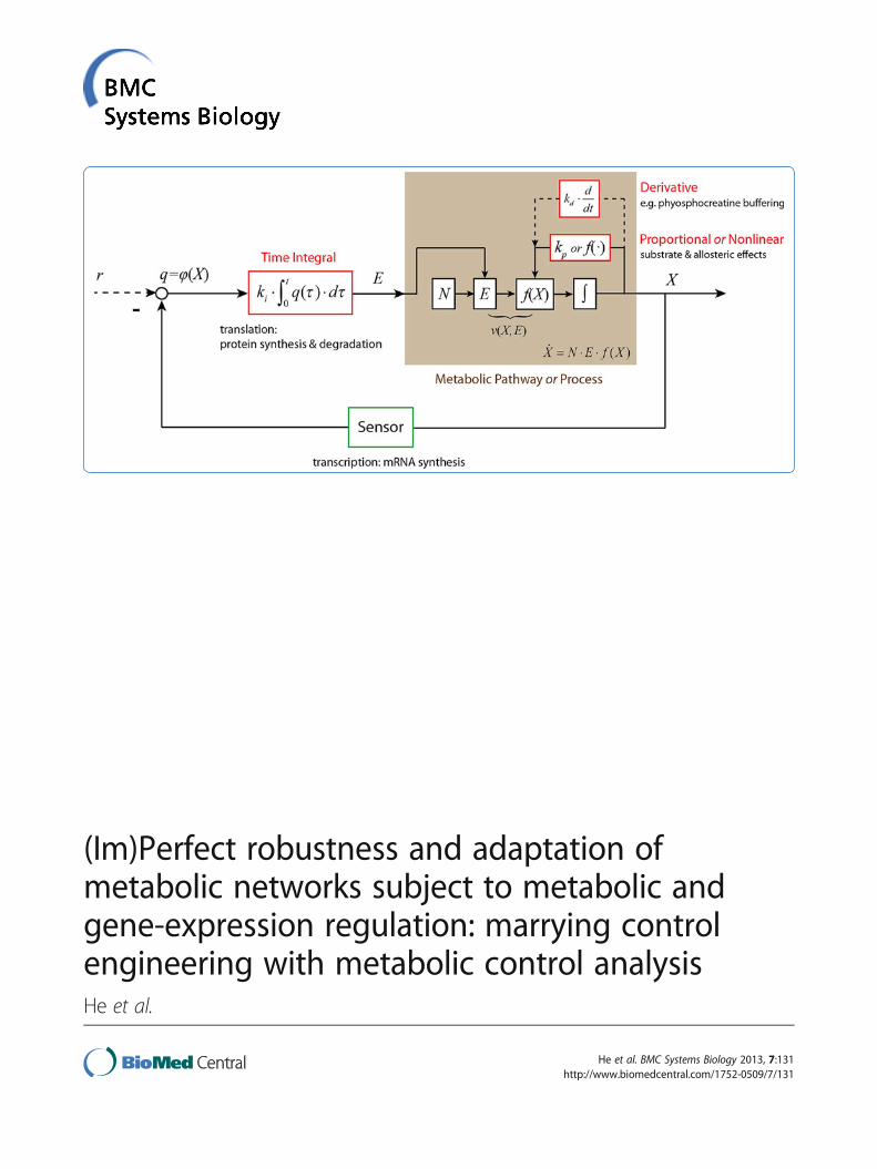
(Im)Perfect robustness and adaptation ofmetabolic networks subject to metabolic andgene-expression regulation: marrying controlengineering with metabolic control analysisHe et al.

He et al. BMC Systems Biology 2013, 7:131http://www.biomedcentral.com/1752-0509/7/131

METHODOLOGY ARTICLE Open Access

(Im)Perfect robustness and adaptation ofmetabolic networks subject to metabolic andgene-expression regulation: marrying controlengineering with metabolic control analysisFei He1,3, Vincent Fromion2 and Hans V Westerhoff1,4,5*

Abstract

Background: Metabolic control analysis (MCA) and supply–demand theory have led to appreciable understanding ofthe systems properties of metabolic networks that are subject exclusively to metabolic regulation. Supply–demandtheory has not yet considered gene-expression regulation explicitly whilst a variant of MCA, i.e. Hierarchical ControlAnalysis (HCA), has done so. Existing analyses based on control engineering approaches have not been veryexplicit about whether metabolic or gene-expression regulation would be involved, but designed different waysin which regulation could be organized, with the potential of causing adaptation to be perfect.

Results: This study integrates control engineering and classical MCA augmented with supply–demand theory andHCA. Because gene-expression regulation involves time integration, it is identified as a natural instantiation of the‘integral control’ (or near integral control) known in control engineering. This study then focuses on robustness againstand adaptation to perturbations of process activities in the network, which could result from environmentalperturbations, mutations or slow noise. It is shown however that this type of ‘integral control’ should rarely beexpected to lead to the ‘perfect adaptation’: although the gene-expression regulation increases the robustness ofimportant metabolite concentrations, it rarely makes them infinitely robust. For perfect adaptation to occur, theprotein degradation reactions should be zero order in the concentration of the protein, which may be rarebiologically for cells growing steadily.

Conclusions: A proposed new framework integrating the methodologies of control engineering and metabolic andhierarchical control analysis, improves the understanding of biological systems that are regulated both metabolicallyand by gene expression. In particular, the new approach enables one to address the issue whether the intracellularbiochemical networks that have been and are being identified by genomics and systems biology, correspond to the‘perfect’ regulatory structures designed by control engineering vis-à-vis optimal functions such as robustness. To theextent that they are not, the analyses suggest how they may become so and this in turn should facilitate syntheticbiology and metabolic engineering.

Keywords: Metabolic control analysis, Control engineering, Transcriptional regulation, Synthetic biology, Robustness

* Correspondence: [email protected] Manchester Centre for Integrative Systems Biology, ManchesterInterdisciplinary Biocentre, University of Manchester, Manchester M1 7DN, UK4Department of Synthetic Systems Biology and Nuclear Organization,Swammerdam Institute for Life Sciences, University of Amsterdam, SciencePark 904, NL-1098 XH Amsterdam, The NetherlandsFull list of author information is available at the end of the article

© 2013 He et al.; licensee BioMed Central Ltd. This is an open access article distributed under the terms of the CreativeCommons Attribution License (http://creativecommons.org/licenses/by/2.0), which permits unrestricted use, distribution, andreproduction in any medium, provided the original work is properly cited.

He et al. BMC Systems Biology 2013, 7:131http://www.biomedcentral.com/1752-0509/7/131

mailto:[email protected]

http://creativecommons.org/licenses/by/2.0

BackgroundWith the development of quantitative functional genomicsapproaches, it has become possible to analyse the cellularadaptation of cell physiology to altered environmentalconditions experimentally, by monitoring changes influxes, metabolites, proteins or mRNAs. Such adaptationstend to occur at multiple regulatory levels if not simultan-eously, then subsequently, depending on the time scales ofobservation [1-3]. In principle, an adaptive change in therate of an enzyme (or flux) can be mediated by changes in(i) the concentration of metabolites (e.g. substrates, prod-ucts and effectors) with direct, cooperative and allostericeffects on the activity of the enzyme [4], (ii) changes in theconcentration of the enzyme through gene-expression al-terations, and (iii) covalent modification via signal trans-duction. The first is termed metabolic (or enzymatic)regulation. The second is known as gene-expression (me-diated) regulation and the third as signal-transduction(mediated) regulation. Because of similar properties, thelatter two types of regulation have been considered to-gether under the term ‘hierarchical regulation’ [2,5,6]. Al-though in this paper only the former two types of adaptivechanges will be discussed explicitly, because of the above-mentioned similarities, the third type is addressed impli-citly. Until now, significant progress has been made on themodelling of genome-scale metabolic networks in micro-organisms integrating metabolic and gene-expressionregulation [7,8]. The steady-state properties of a numberof representative metabolic regulatory mechanisms, suchas end-product inhibition, have been investigated substan-tially both in terms of metabolic control analysis (MCA)[9,10] and by the supply–demand theory championed byHofmeyr and Cornish-Bowden [11-13]. In order to takegene-expression regulation into account, hierarchical con-trol analysis (HCA) [14,15] has been developed as an ex-tension to MCA, but it has not yet been linked up withthe supply–demand theory. Developing such a link wouldseem useful as in quantitative experimental studies gene-expression regulation turned out to be as important asmetabolic regulation [1,2,5,16].The adaptive changes of reaction rates through meta-

bolic and genetic regulation are usually due to feedbackand/or feed-forward mechanisms. In biology, there is aperception that evolutionary optimization has madethese mechanisms perfect. If this were so, this wouldsuggest that such mechanisms might be identical to ‘per-fect’ regulatory mechanisms designed by control engin-eering [17]. Indeed, Csete and Doyle [18] have suggestedthat such a convergent evolution of engineering andbiology may have occurred. In particular, they came withan integral control structure containing both an actuatorunit (corresponding to an integrator) and a controller/sensor unit. They showed that this regulatory structurewould lead to a phenomenon called perfect adaptation

and then proposed that such structures should be com-mon to biology. In systems biology contexts, several bio-chemical processes have been discussed in terms of theircontrol system structures. For example, robust perfectadaptation in bacterial chemotaxis signalling system, inmammalian iron and calcium homeostasis, and in yeastosmoregulation, have been interpreted as integral feed-back control systems [19-22], without however provingthat they corresponded precisely to the very same regu-latory topology or even performance. A recent studyidentified the three different types of control structuresused in control engineering, i.e. proportional, integral,and derivative control, in the regulation of energy me-tabolism [23]. With the exception of [22], the abovework focused only on metabolic regulation, whereas[22] did not compare metabolic regulation with gene-expression regulation. In this study, the integration ofmetabolic and gene-expression regulation plus the in-tegration between Metabolic Control Analysis andControl Engineering will be investigated.Control engineering has examined which network

structures may make adaptation of a network upon asustained perturbation of a network component, ‘perfect’.Perfection was defined as the phenomenon that someimportant system variables (known as ‘controlled vari-ables’) should be completely robust to the perturbations,i.e. with steady states values unaffected by the perturba-tions. Such perfect robustness can be achieved when atime integrator is applied to any variation of the con-trolled variable (or system error). This control feature isknown as ‘integral control’. Through this time integral,the network would continue to change until the con-trolled variable is restored completely to its initial value.Because there must be some compensation for the per-turbation, a different system variable then has to moveaway from its initial state. This so-called ‘manipulatedvariable’ is non-robust (fragile) to the perturbation, butenables the controlled variable to be robust.If the control action is proportional to the variation of

the perturbed variable itself, or a function thereof that iszero when that variation equals zero, the ultimate devi-ation of the controlled variable from its value before theperturbation, will be nonzero. This is the so-called ‘pro-portional control’ of control engineering. Perturbationsmay also result in a sustained oscillation of the con-trolled variable and to prevent this from happening, thethird type of control focused on by control engineeringcan be useful, i.e. so-called ‘derivative control’, which willnot be discussed in this paper, but has been exemplified inreference [23].As mentioned above, the mechanism of integral con-

trol is often referred to as ‘perfect adaptation’. Other au-thors have referred to similar network behaviour thatwas not based on the same integrative mechanism by

He et al. BMC Systems Biology 2013, 7:131 Page 2 of 21http://www.biomedcentral.com/1752-0509/7/131

the same phrase of perfect adaptation. One such case isthat all steps in a metabolic pathway are regulated iden-tically, i.e. their activities being modulated by the samefactor. Tyson et al. [24] referred to this as perfect adap-tation, but the mechanism hinges on precise regulationof various steps, we would suggest to refer to this as‘perfect regulation’ since the adaptation part is not cru-cial. Kacser and Acerenza [25] called this the universalmethod for metabolic engineering. Fell and Thomas [26]proposed that this may be a common motif in biologicalregulation and Adamczyk et al. [27] elaborated it intothe stealthy engineering principle. This paper will notdiscuss this perfect regulation mechanism, but focus onthe robust perfect adaptation mechanism operatingthrough integral control loops.In this work, we shall try to bridge two rather uncon-

nected approaches in analysing regulation of networkproperties. The one is that of control engineering whichhas devised networks structures that lead to perfect or im-perfect adaptation. The other is that of biochemistry withMCA and supply–demand theory, as well as true-to-lifeexamples of intracellular biochemical networks involvingboth metabolism and gene expression. We shall focus onpathways synthesizing precursors for macromolecule syn-thesis (proteins, nucleic acids) in which that precursoroften inhibits an enzyme early in the pathway, both directlyand through gene expression. Such end-product regulatorystructures allow for some simplifications [28]. This makesthem suitable for illustrating our relatively simple conclu-sions that are however valid more generally. We shallhypothesize that because a time integration of protein syn-thesis is involved, gene-expression regulation should be aprime example of integral control, whilst metabolic regula-tion is our candidate for the role of proportional control.We shall then interpret both these steady-state robustnessproperties and the control properties in terms of a newhierarchical supply–demand framework.

MethodsKinetic description and classical control analysisIn this section, we demonstrate that the unique steadystate of a metabolic network under regulations can beanalysed by both the kinetics-based analysis and bymetabolic (or hierarchical) control analysis. A hierarch-ical supply–demand theory linking hierarchical controlanalysis with classical supply–demand analysis, is devel-oped for when gene-expression regulation is active. As aresult the steady state properties of a metabolic networksubject to various regulatory mechanisms can be ana-lysed within a unified theoretical framework.

Basic regulatory architecture and kinetic analysisThe overall regulatory behaviour of a pathway can bedecomposed into a number of elementary structures.

Feedback inhibition by end-product has been reportedfor quite a few metabolic pathways, particularly in anab-olism [29]. Another regulatory motif is the feed-forwardactivation of downstream enzymes (see Appendix A and[30]). In addition, in many metabolic pathways one or afew reactions are product insensitive. The reactions cata-lyzed by hexokinase, phosphofructokinase, and pyruvatekinase in mammalian glycolysis [31] and several steps inthe central carbon metabolism in B. subtilis [28], consti-tute examples. The activities and concentrations of someof these enzymes are regulated by allosteric effectors, co-valent modification or transcription. In this study we takea linear pathway with metabolic and gene-expressionregulation of the first reaction through the end metaboliteas the example of choice [28] (Figure 1). The first reaction(catalyzed by enzyme E1) is assumed to be insensitive toits immediate product. With this example we will be ableto illustrate the essence of the principles we are after.The following differential equations describe this end-

product regulation pathway:

_x2 tð Þ ¼ E1 tð Þ⋅ f 1 x1 tð Þ; xn tð Þ; p tð Þð Þ− E2 tð Þ⋅ f 2 x2 tð Þ; x3 tð Þð Þ_x3 tð Þ ¼ E2 tð Þ⋅ f 2 x2 tð Þ; x3 tð Þð Þ− E3 tð Þ⋅ f 3 x3 tð Þ; x4 tð Þð Þ⋮ ⋮ ⋮

_xn tð Þ ¼ En−1 tð Þ⋅ f n−1 xn−1 tð Þ; xn tð Þð Þ−En tð Þ⋅ f n xn tð Þð Þ_E1 tð Þ ¼ g xn tð Þð Þ− kED⋅E1 tð Þ

ð1ÞHere, we assume that the concentration of the sub-

strate x1 is not influenced by the pathway and that onlyE1 is regulated through gene-expression. xi is the con-centration of ith metabolite, and fi describes the kineticsof the ith reaction. Parameter p corresponds to other fac-tors that could affect the activity of the first enzyme, e.g.co-factors or external metabolic modulators. Such effectson other enzymes are not addressed here. The gene ex-pression function g is here assumed to depend on the ul-timate metabolite only, the latter acting on the synthesisof the first enzyme. More realistic situations involvingthe dynamics of mRNA will be discussed in later sec-tions. This paper is relevant for gene-expression regula-tion in general, i.e. includes regulation at the level oftranscription, translation and post-translational modifi-cation, but our examples will mostly deal with only onetype of these at a time and mainly consider transcriptionregulation. kED is the degradation rate constant of thefirst enzyme. In fast growing organisms and for stableproteins kED may merely represent the dilution effectdue to cell growth and division (i.e. kED = μ, μ denotingthe specific growth rate) [5,28], but in other cases it willdepend on proteolysis, which will be discussed later.By definition of the steady-state in living cells [32], x1(t)

and p(t) are constants at steady state, i.e. x1 tð Þ ¼ �x1 andp tð Þ ¼ �p . Similarly, the concentrations of the enzymes are


constants and equal to �E2;…; �En respectively. Accordingly,if such a constant steady-state regime exists, and it is theunique solution of the following equation:

f 1 �x1; �xn; �pð Þ⋅ g �xnð ÞkED

¼ �En⋅ fn �xnð Þ ð2Þ

which only depends on the first and the end enzymefeatures and is only a function of the end product con-centration xn. Usually, both f 1 �x1; xn; �pð Þ and g(xn) aremonotonically decreasing functions of xn, which de-scribe the negative, metabolic and gene-expressionregulation, respectively. Likewise, fn(xn) is usually amonotonically increasing function of xn. As shown byEquation (2), the steady-state regimen corresponds tothe intersection of the two functions, and is unique dueto the monotonic characteristics of f1, fn and g, as illus-trated in Figure 2.Alternatively, if the ith reaction (i > 1) is product insensi-

tive but the first reaction is not, then f1 is re-defined and it

also becomes a function of x2, while the kinetic functionof the ith step only depends on xi. It can be proven that atsteady state, x2 then only depends on functions f2, …, fiand is independent of fi + 1, …, fn − 1. This conclusion isboth theoretically attractive and practically useful, becausethe steady state properties of an otherwise complex meta-bolic pathway may only depend on a limited number ofenzyme features [33]. This is a case where the complexityof a pathway is limited; its flux and the concentrations ofthe upstream metabolites are only controlled by the prop-erties of the upstream enzymes and the correspondinggenes.We will now examine how metabolic control analysis

and supply–demand theory deal with these types ofmetabolic control structures.

Metabolic regulation: MCA and the supply–demand theoryMetabolic Control Analysis (MCA) has mostly dealtwith the steady state properties of the metabolic part of

Figure 1 The end-product module with gene-expression and metabolic regulation. x1, x2,…, xn represent the concentrations of metabolitesin the pathway; E1, E2,… are the concentrations of enzymes catalysing each reaction. For illustration, only the enzyme of the first reaction (E1) isassumed negatively regulated via both metabolic (allosteric) effect and gene-expression regulation through the end product xn.

Figure 2 Illustration of the unique steady state regimen of a end-product module in terms of kinetics-based analysis.


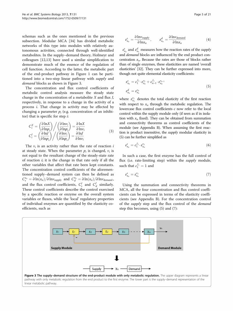
schemas such as the ones mentioned in the previoussubsection. Modular MCA [34] has divided metabolicnetworks of this type into modules with relatively au-tonomous activities, connected through well-identifiedmetabolites. In the supply–demand theory, Hofmeyr andcolleagues [12,13] have used a similar simplification todemonstrate much of the essence of the regulation ofcell function. According to the latter, the metabolic partof the end-product pathway in Figure 1 can be parti-tioned into a two-step linear pathway with supply anddemand blocks as shown in Figure 3.The concentration and flux control coefficients of

metabolic control analysis measure the steady statechange in the concentration of a metabolite X and flux J,respectively, in response to a change in the activity of aprocess i. That change in activity may be effected bychanging a parameter pi (e.g. concentration of an inhibi-tor) that is specific for step i:

CXi ¼ ∂ lnX

∂ lnpi

� ��∂ lnvi∂ lnpi

� �¼ ∂ lnX∂ lnvi

CJi ¼ ∂ lnJ

∂ lnpi

� ��∂ lnvi∂ lnpi

� �¼ ∂ lnJ∂ lnvi

ð3Þ

The vi is an activity rather than the rate of reaction iat steady state. When the parameter pi is changed, vi isnot equal to the resultant change of the steady-state rateof reaction i; it is the change in that rate only if all theother variables that affect that rate been kept constants.The concentration control coefficients of the aforemen-tioned supply–demand system can then be defined asCxn

s ¼ ∂ ln xnð Þ=∂ lnvsupply and Cxnd ¼ ∂ ln xnð Þ=∂ lnvdemand ,

and the flux control coefficients, CJs and CJ

d similarly.These control coefficients describe the control exercisedby a specific reaction or enzyme on the overall systemvariables or fluxes, while the ‘local’ regulatory propertiesof individual enzymes are quantified by the elasticity co-efficients, such as

εsxn ¼ ∂ lnvsupply∂ lnxn

; εdxn ¼ ∂ lnvdemand

∂ lnxnð4Þ

εsxn and εdxn measures how the reaction rates of the supplyand demand blocks are influenced by the end product con-centration xn. Because the rates are those of blocks ratherthan of single enzymes, these elasticities are named ‘overallelasticities’ [32]. They can be further expressed into more,though not quite elemental elasticity coefficients:

εsxn ¼ c J11 ⋅ εv1xn þ c J1n−1⋅ ε

vn−1xn

εdxn ¼ εvnxn

ð5Þ

where εv1xn denotes the total elasticity of the first reactionwith respect to xn through the metabolic regulation. Thelowercase flux control coefficients c now refer to the localcontrol within the supply module only (if seen as if in isola-tion with xn fixed). They can be obtained from summationand connectivity theorems as control coefficients of themodule (see Appendix B). When assuming the first reac-tion is product insensitive, the supply modular elasticity in(5) can be further simplified as

εsxn ¼ c J11 ⋅ εv1xn ð6Þ

In such a case, the first enzyme has the full control offlux (i.e. rate-limiting step) within the supply module,

such that c J11 ¼ 1 and

εsxn ¼ εv1xn ð7Þ

Using the summation and connectivity theorems inMCA, all the four concentration and flux control coeffi-cients can be expressed in terms of the elasticity coeffi-cients (see Appendix B). For the concentration controlof the supply step and the flux control of the demandstep this becomes, using (5) and (7):

Figure 3 The supply–demand structure of the end-product module with only metabolic regulation. The upper diagram represents a linearpathway with only metabolic regulation from the end product to the first enzyme. The lower part is the supply–demand representation of thelinear metabolic pathway.


Cxns ¼ 1

εdxn− εsxn

¼ 1εvnxn− ε

v1xn

CJd ¼ CJ

vn ¼ εsxnεsxn− ε

dxn

¼ 1

1 þ εdxn=εsxn

�� ¼ 11 þ εvnxn=ε

v1xnj j

ð8ÞThese equations show that if the first reaction has

complete flux control within the supply module, the con-trol of steady state end-product concentration and flux areonly functionally depend on two elasticity coefficients, i.e.the ones that correspond to the first and last reactions.When the feedback is very strong, i.e. εv1xn

�� ≫ εvnxn�� , the con-

trol of the demand flux CJd is close to 1. The MCA and

supply–demand simplification thereof discussed in thissection partially explain the state-steady properties of theaforementioned full regulatory system, but only for thecase of metabolic regulation. When including the gene-expression regulation, a more complete interpretation canbe achieved by using the hierarchical control analysis anda new ‘hierarchical supply-demand’ theory as investigatedin the next subsection.

Gene-expression and metabolic regulation: hierarchicalsupply–demand theoryWesterhoff and coworkers have developed hierarchicalcontrol analysis (HCA), an extension of MCA that can takegene-expression regulation and signal transduction intoaccount [14,26]. We shall here implement this by extend-ing the meaning of the elasticity coefficients in the previoussubsection to include regulation through gene expressions.When considering the metabolic part of the network

alone, i.e. if gene expression were always the same, thecontrol on the concentration of intermediate X in a sup-ply–demand system follows (8). If the roles of the synthe-sis and degradation of metabolic enzymes are consideredexplicitly, as illustrated in Figure 4, HCA has to be intro-duced, and the corresponding hierarchical control coeffi-cient becomes:

HXs ¼ ∂ lnX

∂ lnvsupply¼ 1

εdX −�εsX

ð9Þ

Capital H is here used for the hierarchical control co-efficients as defined in Table 1. �εsX is an “overall” elasti-city coefficient, including a classical ‘direct elasticity’only related with metabolic responses (i.e. εsX similar tothe εsxn defined in the MCA in (8)) and an ‘indirect elas-ticity’ due to gene-expression regulation:

�εsX ¼ εsX þ εsEs⋅ cEs

a ⋅ εaX

ð10Þ

The lower case c is used for ‘metabolic control coeffi-cients’, i.e. control coefficients that only take the localnetwork (metabolic, or gene expression but not theircombination) into account. εsEs

is often equal to 1, i.e.when the rate of the reaction in isolation is proportionalto the concentration of the enzyme catalyzing it.Using metabolic control analysis for the gene expres-

sion part of the network, the control coefficient of theprotein synthesis reaction with respect to the concentra-tion of the protein synthesized is:

cEsa ¼ 1

εbEs− εaEs

ð11Þ

Combining the above expressions, one can express thehierarchical coefficient quantifying the control exertedby the supply enzyme on the concentration of the meta-bolic intermediate X in terms of all the elasticity coeffi-cients in the network:

HXs ¼ 1

εdX− εsX−

εsEs ⋅εaX

εbEs−εaEs

¼ 1

εdX þ − εsXð Þ þ εsEs ⋅ −εaXð ÞεbEsþ −εaEsð Þ

¼ −HXd

ð12ÞThe terms in parentheses are usually positive. The

equation shows that the control by supply (i) decreaseswith the absolute magnitudes of the elasticities with re-spect to X of the supply, of the demand, and of the pro-tein synthesis, but (ii) increases for increasing elasticitiesof the protein synthesis and degradation reactions withrespect to the concentration of the enzyme. The equa-tion also shows that for finite non-zero magnitudes ofthe elasticities, the hierarchical control coefficients forcontrol by supply may be decreased by elasticities in thegene-expression network, but is usually not brought

Figure 4 Illustration of hierarchical control. The lower partrepresents a metabolic supply–demand system, in which the supplyis catalyzed by enzyme Es (or enzymes stemming from an operon).The upper part describes the synthesis of enzyme Es in process aand its degradation in process b. Full arrows represent chemicalconversions. Dashed arrows represent allosteric influences orcatalysis. ‘s’ and ‘d’ stand for ‘supply’ and ‘demand’, respectively.


down all the way to zero. The same applies to the con-trol by demand, which is equal to minus the control bysupply.Now let us recall the end-product module with both

metabolic and gene-expression regulatory feedbacks ofFigure 1. As the end product (xn) regulates the first reactionthrough both metabolic regulation and gene-expressionregulation, the corresponding ‘overall’ elasticity (see Table 1)of the first reaction can be expressed as:

�εv1xn ¼ εv1xn þ εv1E1⋅cE1

vTrans ⋅εvTransxn

ð13Þwhere εv1xn denotes the elasticity through metabolic regula-

tion, cE1vTrans denotes the control of gene expression (i.e. tran-

scription and translation) on the concentration of the firstenzyme [15,35]. By replacing the εv1xn in (7) with the more

complete expression (13), i.e. using εsxn ¼�εv1xn , the hier-archical control coefficient Hxn

s can be expressed into elas-ticity coefficients, in a similar manner as (12). Since bothmetabolic and gene-expression regulation constitute nega-tive feedbacks, εsxn is negative and becomes more negativewith increasing xn due to increasing product inhibition.

εdxn is positive and decreases asymptotically to zerowith increasing xn. Therefore, the relationship betweenthe reaction rate and end product concentration can bedescribed in terms of the elasticities as depicted inFigure 5. Figure 5 explains the unique steady-stateresults obtained from classical steady state analysis(see Figure 2).An illustration of the supply–demand relationship

similar to Figure 5 has been presented in [13]. However,here we extend the interpretation of the system and cor-responding elasticity coefficients to the more generalcase that includes gene-expression regulation. As an ex-tension to the classical supply–demand theory, the ana-lysis given in this section can be named the ‘hierarchicalsupply-demand’ theory.

Control engineeringThe discipline of Control Engineering first identifies aso-called controlled variable, which it sees as the outputof the system. In metabolic biochemistry, output oftenrelates to a flux, but can also be the concentration of animportant metabolite in the pathway. Control engineer-ing next examines the various categories of mechanismthat may contribute to the capability of the network of

Table 1 The list of symbols and definitions

Symbol Definition & comments

Cfi or c

fi Metabolic control coefficients as defined in (3). f is the system function of interest (i.e. a particular flux, Jj, or a metabolite concentration X).

Lowercase c is used to represent control within a local network (e.g. supply module). The index i refers the process that is controlling.

Hfi Hierarchical control coefficient. Its mathematical definition is in the same form as metabolic control coefficients in (3), but the system

under study can be more general. MCA only studies the control in a metabolic pathway or a signal transduction cascade, but not theircombination. HCA investigates the control in a hierarchical regulatory network with interactions at different levels, i.e. metabolic, signaltransduction, and gene-expression.

ℜfi MCA (or HCA) based robustness coefficient.

ℜfi≡

1

∂ lnf∂ lnei

� �≡ 1Cfior 1

Hfi.

Ffi Fragility coefficient. It is the inverse of the robustness coefficient and identical to the control coefficient. Ffi≡∂ lnf∂ lnei

≡ 1ℜf

i≡Cf

i or Hfi :

εvjxi Elasticity coefficient defined in MCA. It denotes the immediate influences of metabolite xi with respect to the reaction rate in the jth stepin the pre-steady state.

εsxi or εdxi Elasticity coefficient of metabolite xi with respect to the metabolic supply (s) or demand (d) module, as defined in (4).

�εvjxi ,�εsxi

(or �εdxi )The overall elasticity (see [32]) for a reaction step under both metabolic and gene expression regulation, or the overall elasticity in ahierarchical supply or demand module.

vTrsc orvTrnl

Reaction rate of transcription or translation

vRD or vED Reaction rate of mRNA or protein degradation

kRD or kED mRNA or protein degradation rate constant

kiproteolysis Rate constant of ith order proteolysis

μ The cells’ specific growth (division) rate

E Concentration of enzyme

X or xi Concentration of intermediate metabolite

R Concentration of mRNA

r Reference signal.


maintaining the controlled variable close to its originalsteady state value when the system is subject to a sus-tained perturbation. The ‘error (function)’ is the devi-ation (δX) of the value of the controlled variable (X)from its value before the perturbation, or the differenceto a reference signal r. The network ‘adapts’ to the per-turbation of the controlled variable, i.e. to the errorfunction, in a so-called ‘control action’. RNA polymeraseplus the ribosomes that together translate changes in theconcentration of metabolites to changes in gene expres-sion, or direct metabolic regulation of the activity of anenzyme correspond to such control actions. The outputof the control action (or of the ‘controller’) is oftennamed the manipulated variable. In metabolism, reac-tion rates v(X, E) are variables manipulated either by theconcentration of metabolites (f (X)) or by the concentra-tion of the enzyme that catalyses the reaction concentra-tion (E). A mechanical control system often includes anactuator that converts the control signal into some kindof mechanical motion. For a biochemical system dis-cussed in this study, this may correspond to the enzymecatalysing the reaction synthesizing or degrading X. Usu-ally there exists a sensor measures the controlled variableand translates its error function into the input signal ofthe controller. In a gene-expression regulation, the tran-scription factor can be regarded as the sensor.The three most widely used categories of control

are the proportional, integral, and derivative (PID)control mechanisms [17]. They differ depending onwhether the control system’s response is a function ofthe ‘error function’ itself, the time integral thereof orthe time derivative thereof, respectively. In systemsbiology literature, the proportional control mechanism

has already been referred to in terms of metabolicregulation [19,20,23] (e.g. feedback inhibition). However,when Control Engineering discusses proportional controlmechanisms, response is proportional to the error func-tion. In actual biochemistry, enzyme activity is rarely alinear function of the concentrations of metabolites X,which includes the enzyme’s substrate, its product andallosteric modifiers. MCA accommodates this nonlinearityby allowing the elasticity coefficient to differ from 1.Metabolic regulation by the ‘error function’, is part of thenonlinear dynamics of the process or system, i.e. f (X),both conceptually and in the mathematical modelling. Itwould seem therefore that the proportional control ofControl Engineering can be nonlinear in biochemicalnetworks.Integral control action through the accumulation of

molecules in the metabolic process has also been reported[19,20,23]. Here the systems response should be a functionnot of the error function itself but of the integral of thaterror function. In the present study we examine gene-expression regulation from this point of view, since pro-tein synthesis requires time integration and depend on theerror function, and because changes in protein concentra-tion directly affect the rate of the reaction the protein maycatalyzes. We may expect that this integral control some-how corresponds to the ‘indirect elasticities’ of HCA.Whether indeed gene-expression regulation correspondsto an exact (or ideal) integral control mechanism will befurther discussed in the Results and Discussion section.Whether there exists a derivative control action andwhether it relates to a specific type of regulation in a meta-bolic pathway will not be investigated in this paper. Refer-ence [23] already identified an example.

Figure 5 Illustration of the steady state properties of a supply-demand system in terms of changes in the flux, intermediateconcentration and elasticity coefficients.


Considering the dynamics of a metabolic system, wecan write the time dependence of the concentrations ofits metabolites as:

_X ¼ N⋅v X;Eð Þ ¼ N⋅E⋅f Xð Þ ð14Þ

N is the stoichiometry matrix. E is a diagonal matrixwith the concentrations of the enzymes that catalyse thevarious reactions along its diagonal. f (X) is a vectorfunction of the concentrations of the metabolites andkinetic parameter values. The regulated metabolic path-way can be described in terms of a closed-loop feedbackcontrol system, as indicated in Figure 6, in which kp, kiand kd are the PID control parameters. We here notethat Figure 6 and subsequent figures refrain from bio-chemical detail. This is because the analysis in thepresent paper aims at obtaining a set of conclusions withgeneral significance. Being specific in the schemes weuse as illustrations would detract from this aim.When considering a sustained perturbation γ∙δp (e.g.

change in a parameter p) and denoting by δ the (small)deviation from the steady state prior to this perturb-ation, the time dependent variation in the metaboliteconcentrations may be observed:

δ _X ¼ N ⋅ δv X; Eð Þ ¼ N⋅Ess⋅f ′ Xð Þ⋅ δX þ N⋅ f Xð Þss⋅ δE þ γ⋅ δp

ð15Þ

The subscript ss refers to the steady state values. Bysubstituting the time integration of gene expression, i.e.

ki⋅Z t

0q τð Þ⋅dτ , for δE, and assuming the proportional

and derivative actions a part of the metabolic process(14),

δ _X¼N⋅ Ess⋅ f ′ Xð Þ⋅ δX þ N⋅ f Xð Þss⋅ ki⋅Z

0δφ Xð Þ⋅ dt þ γ⋅ δp

ð16Þ

This describes the overall dynamics of a closed-loopmetabolic system under perturbation as a sum of threeterms. The first term of these is a nonlinear function of(or in first order proportional to) the perturbation of thecontrolled variable (i.e. the error function) δX. This termdescribes all the direct elasticities, including non-regulatorysystem kinetics such as substrate and product effects, and(other) metabolic regulation such as allosteric activation.The second term corresponds to a time integral of a func-tion of the perturbation of the controlled variable δX, andcan also depend on other system variables as discussed inthe Results and Discussion section.We shall now examine whether these two terms in the

equation (16), correspond to the proportional and integralcontrol loops of Control Engineering.

Figure 6 The closed-loop control structure of a metabolic pathway subject to various types of regulation. There are three types offeedback control mechanisms: i) proportional or nonlinear control that is related to the substrate or allosteric effects; ii) derivative control that canbe related with signalling, e.g. phyosphocreatine buffering; and iii) integral control introduced by gene-expression regulation because proteinsynthesis requires time integration. The former two control loops i) and ii) are often modelled together with the dynamics of the metabolicprocess. Here, metabolite concentration X is the output of a metabolic process and is the controlled variable of different control loops. Reactionrates v(X,E) are the manipulated variables because they are functions of both enzyme concentration E, i.e. the output of integral control loop(gene-expression regulation), and metabolic process (f(X)), i.e. the outputs of proportional/nonlinear and derivative control loops (metabolicregulation or signalling). Here, the integral control input q(t) is a function of the controlled variable (q(t) = φ(X(t)) or the difference (or error)between the controlled variable and a reference signal (r).


Results and discussionA simple example of combined metabolic andgene-expression regulation of an important intracellularprocess: ATP (energy) metabolismLet us consider the simple example given in Figure 7, i.e.a two-step pathway with ATP and ADP as combinedintermediate and with the expression of the gene encod-ing the first enzyme E increasing in proportion to theconcentration of ADP. The ‘moiety conservation sum’ Cis the sum of the concentrations of ATP and ADP and aconstant here (i.e. C = [ATP] + [ADP]) because the reac-tions only convert the one into the other. The metabolicregulation addresses the interplay between the supplyand demand processes (s and d).The dynamics of ADP and enzyme E are here assumed

to follow mass action kinetics:

d ADP½ �=dt ¼ −ks⋅E⋅ ADP½ � þ kd⋅ C− ADP½ �ð ÞdE=dt ¼ ka⋅ ADP½ �−kb⋅E−k0

ð17Þ

The degradation of the enzyme is here written as thesum of two terms, which will serve to emphasize the im-plication of this degradation to be independent (for kb = 0)or dependent (for k0 = 0; see below) on the enzyme con-centration. The first order degradation rate reflects the

assumption that there is a rather unspecific protease activ-ity for which the particular enzyme E we are consideringhere is a minority substrate. The zero order degradationwould reflect a case where there is a specific proteasesystem for enzyme E (e.g. an ubiquitination followed by ageneric protease) that is saturated by the already highconcentration of the enzyme relative to the KM of the ubi-quitin transferase. In (17) all rate constants are considerednon-negative and k0 = 0 whenever E is non-positive. Theclosed-loop control system structure of the pathway canbe represented as in Figure 8.The control system diagram suggests that the ADP

concentration is the controlled variable and the en-zyme concentration E a manipulated variable in thegene-expression control loop. The zero order degrad-ation rate k0 can be treated as a reference signal tothe system. The metabolic regulation is included as apart of the ADP kinetic process. By considering aperturbation of kd from its steady state value (i.e.δkd), and reformulating the kinetics of ADP and E(see Appendix C), we have

δ ADP½ �: ¼ − ks⋅Ess þ kdð Þ⋅ δ ADP½ �− ks⋅ ADP½ �ss⋅

Z ∞

0

ka⋅ δ ADP½ �− kb⋅ δEð Þ⋅ dtþ C− ADP½ �ss�

⋅δkdð18Þ

Comparing this to a general closed-loop controlsystem (16), with ADP for X, we recognize on the right-hand side first a proportional response term, then anintegral response term, and then the perturbation term.The proportional response corresponds to the direct‘elasticity’ of the supply and demand reactions with re-spect to the error function δ[ADP], which is a metabolicand instantaneous regulation. The integral response isrelated to the protein synthesis and degradation and thusto gene-expression regulation.When the degradation of enzyme is zero order in terms

of E (i.e. when kb = 0), the gene-expression regulation be-comes an ideal integral control loop, and the metabolicnetwork can exhibit robust perfect adaptation to the exter-nal or parametric perturbations. This can be understoodby requiring (18) to be valid in a steady state, i.e. with timeindependent values for [ADP] and E. Because the time in-tegral reaches to infinity this requires that the argument ofthe integral, i.e. ka ⋅ δ[ADP] − kb ⋅ δE, must equal zero. Themechanism for this perfect adaptation is that after the per-turbation the concentration of the enzyme will vary untilit makes the time dependences equal zero by itself, forgo-ing the more usual process in metabolic regulation thatchanges in the controlled variable arrange for the steadystate to be re-attained in the presence of the sustainedperturbation.

Figure 7 ATP energy metabolism in a two-step pathway withgene-expression regulation. The lower part represents a simplifiedATP/ADP energy metabolism process, in which ADP acquires energyfrom the supply process (s) (i.e. phosphorylation) and produce ATP;also ATP can release energy in the demand process (d) (i.e.hydrolysis) and be converted to ADP. The supply is catalyzed byenzyme E (or enzymes stemming from an operon). The upper partdescribes the synthesis of enzyme E in process a and its degradationin process b.


For the more general case where the enzyme degradationmay depend on the enzyme’s concentration, the (hierarch-ical) control of the enzyme level by the demand reactioncan be expressed in terms of the kinetic parameters andthe steady-state ADP concentration (see Appendix C):

HEkd ¼ ∂ lnE

∂ ln kd¼

ks⋅kakb

⋅ ADP½ �ss� 2

kd⋅C þ ks⋅ ADP½ �ss� 2⋅ kakb

¼ 1−1

1 þ ks⋅ ADP½ �ssð Þ2kd⋅C

⋅ kakbð19Þ

The flux control exercised by the demand reaction isquantified by:

HJkd

¼ ∂ ln J∂ ln kd

¼ 1−ADP½ �ssC

1 þ ks⋅ ADP½ �ssð Þ2kd⋅C

⋅ kakb

ð20Þ

Both the control of enzyme level and the control of de-mand flux by the perturbation equal 1 minus a hyperbolicfunction of kb. For the ideal integral control scenario ofkb = 0, the enzyme concentration E tracks the activity ofthe pathway degrading ATP perfectly, i.e. HE

kd ¼ 1. Moreimportantly, the pathway flux perfectly tracks the perturb-ation in the demand flux and HJ

kd¼ 1. This is the case of

robust perfect adaptation. For other cases when kb ≠ 0, theadaptation of the pathway to the perturbation will not beperfect and both control coefficients are smaller than 1.Also the robustness coefficient [36] of the ADP con-

centrations vis-à-vis perturbations in the demand reac-tion can be expressed in terms of kinetic constants andthe concentration of ADP (see Table 1 for definition):

ℜ ADP½ �kd

¼ 1∂ ln ADP½ �∂ ln kd

¼ kd⋅C þ ks⋅ ADP½ �ss� 2⋅ kakb

C− ADP½ �ss�

⋅kdð21Þ

Only if kb = 0, kd = 0, or [ATP]ss =0, the ADP and ATP

are perfectly robust (ℜ ADP½ �kd

¼ ∞ ) versus perturbations.

The fragility [36] of the ADP concentration vis-à-vis per-turbation in the demand reaction, which is the inverse ofthe robustness, can be quantified by the concentrationcontrol coefficient for the concentration of ADP with re-spect to the degradation process. It reads as:

F ADP½ �kd

≡1=ℜ ADP½ �kd

¼ ∂ ln ADP½ �∂ ln kd

¼ C− ADP½ �ssC þ ADP½ �ss

� 2⋅ ks⋅kakd ⋅kb

ð22Þ

This fragility is a hyperbolic function of the first orderdegradation rate constant of the enzyme and hence zerowhen that degradation is zero-order (see Figure 9 for il-lustration). The fragility has the ATP/(ADP + ATP) ratioas its maximum value (hence the minimum robustnessequals the (ADP + ATP)/ATP ratio). Half maximum fra-gility is attained for:

kb ¼ ADP½ �ss� 2

C⋅ks⋅kakd

ð23Þ

This means that the fragility may be low for a substan-tial magnitude of the first order rate constant of proteindegradation if the rate constant for protein synthesis isalso high. The control coefficients for the enzyme levelHE

kd and the demand flux HJkd

attain a maximum of 1and a value of ½ when the fragility of ADP is halfmaximal.These conclusions can be generalized somewhat by

directly implementing HCA and hierarchical supply–de-mand result given in (12). For the above model the elas-ticity coefficients assume the following magnitudes:

εsADP½ � ¼ εaADP½ � ¼ εsE ¼ 1

εaE ¼ 0

εdADP½ � ¼ −ADP½ �

C− ADP½ �

ð24Þ

Figure 8 Control system structure of ATP energy metabolism. k0 and kb are the zero and first order protein degradation rate constants. ka isthe protein synthesis rate constant.


For the robustness of the ADP concentration vis-à-visincreased demand one then finds:

1

H ADP½ �d

¼ −εdADP½ � þ εsADP½ � þεsE⋅ε

aADP½ �

εbE−εaE

¼ CC− ADP½ � þ

1

εbE

ð25ÞThis shows that robustness is infinite if the enzyme

degradation reaction is zero order (i.e. εbE ¼ 0), and thatthe robustness becomes smaller with increasing order(elasticity) of this reaction.The most important conclusion here is that there is

no discontinuity in the ability of integral control loopsto lead to good adaptation. The closer the degradationof the enzyme that enables the adaptation is to a zero-order reaction, the stronger its tracking of the perturb-ation in the demand flux, and the higher the robustnessof the variable that is to be kept homeostatic. Importantperhaps is the phenomenon that the robustness is notdetermined by the magnitude of the degradation reac-tion but by its kinetic order (i.e. elasticity of effective Hillcoefficient). The corresponding conclusions pertain tothe tracking of the demand by the enzyme level E andthe control of the pathway flux by the demand reaction.A further issue in control engineering is the robustness

of systems versus perturbations at various frequencies.In engineering, an airplane wing has to be robust to vari-ations of air pressures at high frequencies, as well at lowfrequencies. In order to achieve this combined robust-ness, different control loops may have to be put in placesimultaneously, although a trade-off limits what one can

do [18]. In systems biology, this can be illustrated for theend-product feedback regulation in Figure 1. If the fluxdemand of the pathway increases rapidly, the concentra-tion of the end product decreases rapidly and as a resultof the direct allosteric product inhibition effect, the ac-tivity of the first enzyme will increase quickly too. Thismetabolic control of enzyme activity is a fast actuator ofthe system. However, if there is a further increase in theflux demand, the first enzyme may ‘lose’ its control cap-acity since its activity may be approaching its maximumcapacity (kcat). At this stage, the system may thenundergo a second ‘adaptation’ through gene expressionwhich should be expected to be slower because the cellhas to produce enzyme, but still ultimately lead to anincrease in the concentration of the first enzyme. Thisincrease should then decrease the direct metabolicstimulation of the catalytic activity of the enzyme dis-cussed above. In this sense, the regulation of the first en-zyme of the pathway is bi-functional in dynamic terms[18]: The metabolic regulation rapidly rejects high fre-quency perturbations but possibly with small amplitudeor capability, while the gene-expression regulation isslow to adapt, but may be able to reject very large con-stant perturbations.

Conditions for integral and pseudo-integral control:end-product pathwayIn this section, we recall the end-product module ex-ample (of which the simple ATP metabolism example isa special case) to analyse gene-expression regulation in amore general metabolic pathway. In particular, the con-ditions will be identified for which the gene-expressionregulation constitutes ideal integral control or pseudo-integral control will be discussed. A simple but represen-tative end-product example is given in Figure 10, i.e. alinear pathway with three metabolites, where for all thethree enzymes the gene expression is regulated by thelast metabolite. The kinetic model of this example withall the parameters is provided in [5].Gene transcription and translation are modelled here

explicitly by further including the dynamic function ofmRNA as

_R ¼ vTrsc− vRD ¼ gTrsc x3ð Þ− kRD⋅R_E ¼ vTrnl− vED ¼ gTrnl Rð Þ− kED⋅ E ð26Þ

Here gTrnl(R) = kTrnl ⋅ R is a function of mRNA concen-tration R. kED essentially consists of three parts. Oneterm is due to dilution, which is proportional to the spe-cific cell growth rate μ. The other terms correspond toproteolysis, as below:

kED ¼ μ þ k1proteolysis þ k0proteolysis=E ð27Þ

Figure 9 The fragility of the ADP concentration with respect toperturbation in the demand flux as the protein degradationrate constant kb changes. The fragility is zero when the kb is zero;the maximum fragility equals the ATP/(ADP + ATP) ratio. The solidline represents the fragility under a ATP/(ADP + ATP) ratio of 0.5 atsteady state; the dot-dash line is with a ratio of 0.4; and the dashedline is with a ratio of 0.6. The half maximum fragility is attained whenkb satisfies (23), e.g. kb = 0.3333 under a ATP/(ADP + ATP) ratio of 0.5.


The final term denotes the zero order proteolysis aswould be caused by proteases that are saturated with theprotein of interest. We here assume that the specificgrowth rate μ is independent of the activity of the path-way under study, an assumption that is sometimes butnot always realistic. Since after multiplying with E thelast term is independent of the protein concentration,it is convenient to move this term into the protein syn-thesis function gTrnl(R). Hence, the new protein degrad-ation rate can be defined as,

kED ¼ μ þ k1proteolysis ð28Þand the protein dynamics can be re-written as,

_E ¼ gTrnl Rð Þ− kED⋅E¼ kTrnl⋅R− k0proteolysis� �

− μ þ k1proteolysis� �

⋅ Eð29Þ

In the exponential growth phase or if proteolysis isfirst order (i.e. kED ≠ 0), the above pathway examplecorresponds to a pseudo- or non-integral controlscenario. The control structure of the regulatory system isthen given by Figure 11. The dynamics of the ‘sensor’is decomposed here by addressing both transcriptionand the translation through mRNA. At steady state,often gTrnl(R)ss = kED ⋅ Ess ≠ 0. Therefore, after perturb-ation of a system parameter (i.e. kinetic constants),the new steady state values of x3, R, and gTrnl(R) willno longer be the same as the old steady state values,which indicates that then the regulatory system doesnot achieve perfect adaptation. However, when kTnD isvery small, near-perfect adaptation behaviour shouldbe observed.

An ideal integral control scenario will happen onlywhen cell enters a stationary phase and there only existszero order proteolysis, i.e. kED ¼ μ þ k1proteolysis ¼ 0 . In

such case, at steady state, gTrnl(R)ss ≡ 0 due to integralcontrol, and R and x3 will also always keep the sameconstant values at steady state, no matter how the sys-tem parameters are perturbed. The adaptation of thesystem is then perfect in the sense of making the systemproperties R and x3 robust against the perturbations.The functions gTrnl(·) and gTrsc(·) can also be multivari-ate, i.e. contain other system variables. Only if those var-iables do not depend functionally on the proteinconcentration (E), the adaptation vis-à-vis perturbationsof the system kinetic parameters will remain perfect.The ideal integral control scenario that we considered

above led to the perfect robustness of certain systemvariables with respect to certain (external or parametric)perturbations. A second aspect of the perfect adaptationscenario is the perfect tracking by a second system vari-able of perturbations. Perfect tracking means that therelative change in the variable is identical to the relativechange in the perturbing parameter. If the parameter isthe activity of a process, then this means that the corre-sponding control coefficient is equal to 1. The perfecttracking of references and the perfect robustness of con-trolled variables to perturbations are two aspects of inte-gral control systems, i.e. the two features can beobserved simultaneously for the same system. A specificpathway then shows perfect robustness of a system vari-able vis-à-vis multiple perturbations (or parameters) butperfect tracking with respect to only a limited set of pa-rameters (e.g. a reference signal r).

Figure 10 A linear end-product pathway with gene-expression and metabolic regulation. The metabolites are denoted by xi, mRNA by mRand enzymes by E. S and P are the external metabolites. Metabolite x3 inhibits the rate of enzyme 1 through metabolic regulation and thesynthesis of enzyme 1, 2 and 3 through gene-expression regulation. Enzymes 1, 2 and 3 are encoded on the same operon.


For the aforementioned example, the zero order proteoly-sis can be regarded as a ‘reference’ signal r ¼ k0proteolysis . Ef-

fectively perturbation of this rate constant corresponds toan external perturbation of protein synthesis. The effect isthat even at an ideal integral control case, i.e. when kED = 0,the steady state concentration of mRNA will not become 0.Rather, it will always ‘track’ the reference r (i.e. R = r/kTrnl ≠0) whenever _Ess ¼ 0. The reference tracking control systemstructure is included in Figure 11 with reference r referredto by a dashed arrow, and with gTrnl(R) then representingkTrnl ⋅ R.

Practical concerns and assumptions on degradation rateconstant kEDIn general, kED ¼ μ þ k1proteolysis > 0 . It may seem that

the condition of integral control can be approached,when either i) kED < < α with α a very small positivevalue, or ii) kED < < kTrnl (or kED · E < < gTrnl(R)). In thelatter case, for the level of protein to remain bounded,there should be a background degradation rate of theprotein independent of the concentration of that protein.This would be so if:

μ þ k1proteolysis≪k0proteolysis=E ð30Þ

During the exponential growth phase of bacteria suchas E. coli less than 1% of a protein may be degraded dur-ing a cell division cycle [37]. Consequently the majorterm in the protein degradation is the dilution term μand this term is generally very small. Indeed, by defin-ition, eμ ⋅ T = 2, where T is the doubling time of the bac-teria and then μ = ln2/T. Practically, the smallest value

for T is close to 20 minutes [38], which correspondingto the fastest growth rate of E. coli:

μ≈ ln 2= 20 � 60ð Þ ¼ 5:8 � 10−4 s−1� ð31Þ

Such a growth rate in microbes such as E. coli andyeast, which is fast for organisms but slow at the timescale of RNA and protein synthesis, produces a small ef-fective degradation rate constant for the proteins. Belowwe shall see whether such a small degradation rateconstant suffices to produce near-perfect adaptationbehaviour in practice, which would be interpreted asa quasi-perfect integral control system.

Simulation studyIn this section, both the integral and the non-integral con-trol scenarios are simulated based on the example given inFigure 10 with all the kinetic parameters given in [5]. Threedifferent systems are considered, with kED = 0, 0.2, and 0.4,respectively. All three systems are simulated from the sameinitial condition. The concentration changes of mRNA, Eand x3 are shown in Figure 12. After a period of time (e.g.30 seconds) the three systems reach different steady states.Then at 50 seconds we perturb one system parameter (i.e.the kcat of the third reaction) by 20% for all three cases.After a while the three systems reach new steady states.After perturbation only the system with zero order proteindegradation (i.e. kED = 0), returns to the same steady statevalues for mRNA and x3 as those before perturbation,which indicates perfect adaptation: this is an ideal integralcontrol system. In this case the manipulated variable,the enzyme level E, varies strongly. Its adaptation enablesx3 and mRNA to be completely robust vis-à-vis the

Figure 11 Control system structure of a pseudo-integral or an ideal integral control problem. hTrsc(·) denotes the transcription process.gTrnl(·) denotes the rate of protein synthesis. The pseudo-integral control system becomes an ideal integral control only when the dashed lineconnecting the degradation rate kED is removed.


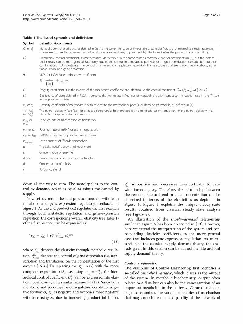
perturbations of the kcat of the third reaction. In the othertwo cases (i.e. kED = 0.2 or 0.4), the change in enzyme levelis smaller, but the new steady state values of mRNA andx3 deviate from their previous steady-state values andadaptation is not perfect. However, the deviations are notlarge; only 3% for x3 and 4% for mRNA when kED = 0.2,and 4% for x3 and 8% for mRNA when kED = 0.4.Now let us consider the reference tracking scenario.

The responses of enzyme and mRNA to a 20% perturb-ation in the protein stability (r) at t = 50 seconds, aregiven in Figure 13 for three different rate constants ofenzyme degradation kED. Only when kED = 0 the mRNAconcentration tracked the reference value with zerosteady state ‘deviation’. This indicates the existence of aperfect integral action of the feedback regulatory system.When kED was not equal to zero (i.e. kED = 0.2 or kED =0.4), the mRNA response did not track the reference sig-nal, indicating that in these two cases the controller ofthe system was not an ideal integral controller, althoughit changed less than did the reference signal.

HCA and an hierarchical supply–demand interpretationThis simulation example can be represented by a hier-archical supply–demand structure such as in Figure 4.To obtain ideal integral control, both protein synthesisand protein degradation should be independent of theconcentration of the protein that is being degraded (i.e._E ¼ gTrnl Rð Þ). Since this implies that protein degradationis zero order in protein concentration:

εbEs¼ εaEs

¼ 0 ð32ÞSo that the hierarchical control coefficient of the me-

tabolite concentration becomes

HXs ¼ 1

εdX−εsX−

εsEs ⋅εax

εbEs−εaEs

¼ 1

εdX þ −εsXð Þ þ εsEs ⋅ −εaxð Þ0

¼ 0

ð33Þ

Here εaEs¼ εvTrnlE , εbEs

¼ εvEDE , HXs ¼ Hx3

3 for the biosyn-thetic pathway example. Because the hierarchical controlby supply and demand must add to zero (due to theconcentration control summation law [15]), also thecontrol by demand on the metabolite concentration be-comes precisely equal to zero in the zero order proteindegradation case.

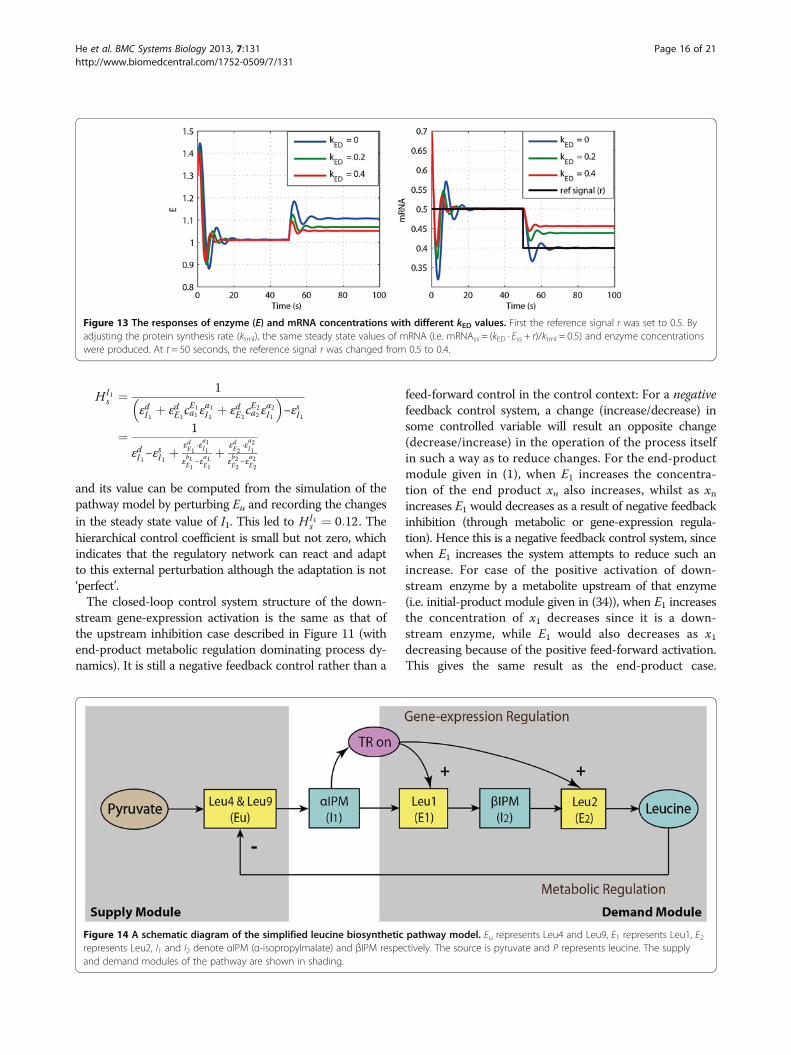
Feed-forward activation: a case study of a leucinebiosynthetic pathwayIn previous sections, either a metabolic intermediate(ADP) or a penultimate product (xn) inhibited or re-pressed upstream enzymes. In this section a differentregulatory structure is investigated, one in which ametabolite activates downstream enzymes throughgene-expression. A simplified mathematical model de-scribing the leucine biosynthetic pathway in Saccharo-myces cerevisiae [39] is used to demonstrate that theanalysis integrating hierarchical supply–demand the-ory and control engineering continues to apply. Thepathway converts pyruvate to leucine by the sequen-tial reactions described in Figure 14. There are twomajor regulatory mechanisms in the pathway. One isa metabolic feedback inhibition of Leu4 and Leu9 byleucine, which is an end-product module similar tothe ones discussed above. The other is the transcrip-tional (gene-expression) activation of downstream en-zymes Leu1 (E1) and Leu2 (E2) by αIPM (I1) (throughtranscription factor Leu3), which we shall call initial-product modules (see Appendix A and Figure 17).The model predictions fit the experimental data andall the parameter values have been estimated andprovided in [39].The hierarchical control coefficient quantifying the con-

trol of supply enzymes Es with respect to the concentrationof I1 (αIPM) can be expressed into the various elasticity co-efficients (see also Figure 15),

Figure 12 The responses of mRNA, enzyme (E), x3 under perturbation with different kED values.


HI1s ¼ 1

εdI1 þ εdE1cE1a1 ε

a1I1 þ εdE2

cE2a2 ε

a2I1

� �−εsI1

¼ 1

εdI1−εsI1 þ εdE1

⋅εa1I1εb1E1−εa1E1

þ εdE2⋅εa2I1

εb2E2−εa2E2

and its value can be computed from the simulation of thepathway model by perturbing Eu and recording the changesin the steady state value of I1. This led to HI1

s ¼ 0:12. Thehierarchical control coefficient is small but not zero, whichindicates that the regulatory network can react and adaptto this external perturbation although the adaptation is not‘perfect’.The closed-loop control system structure of the down-

stream gene-expression activation is the same as that ofthe upstream inhibition case described in Figure 11 (withend-product metabolic regulation dominating process dy-namics). It is still a negative feedback control rather than a

feed-forward control in the control context: For a negativefeedback control system, a change (increase/decrease) insome controlled variable will result an opposite change(decrease/increase) in the operation of the process itselfin such a way as to reduce changes. For the end-productmodule given in (1), when E1 increases the concentra-tion of the end product xn also increases, whilst as xnincreases E1 would decreases as a result of negative feedbackinhibition (through metabolic or gene-expression regula-tion). Hence this is a negative feedback control system, sincewhen E1 increases the system attempts to reduce such anincrease. For case of the positive activation of down-stream enzyme by a metabolite upstream of that enzyme(i.e. initial-product module given in (34)), when E1 increasesthe concentration of x1 decreases since it is a down-stream enzyme, while E1 would also decreases as x1decreasing because of the positive feed-forward activation.This gives the same result as the end-product case.

Figure 14 A schematic diagram of the simplified leucine biosynthetic pathway model. Eu represents Leu4 and Leu9, E1 represents Leu1, E2represents Leu2, I1 and I2 denote αIPM (α-isopropylmalate) and βIPM respectively. The source is pyruvate and P represents leucine. The supplyand demand modules of the pathway are shown in shading.

Figure 13 The responses of enzyme (E) and mRNA concentrations with different kED values. First the reference signal r was set to 0.5. Byadjusting the protein synthesis rate (ktrnl), the same steady state values of mRNA (i.e. mRNAss = (kED · Ess + r)/ktrnl = 0.5) and enzyme concentrationswere produced. At t = 50 seconds, the reference signal r was changed from 0.5 to 0.4.


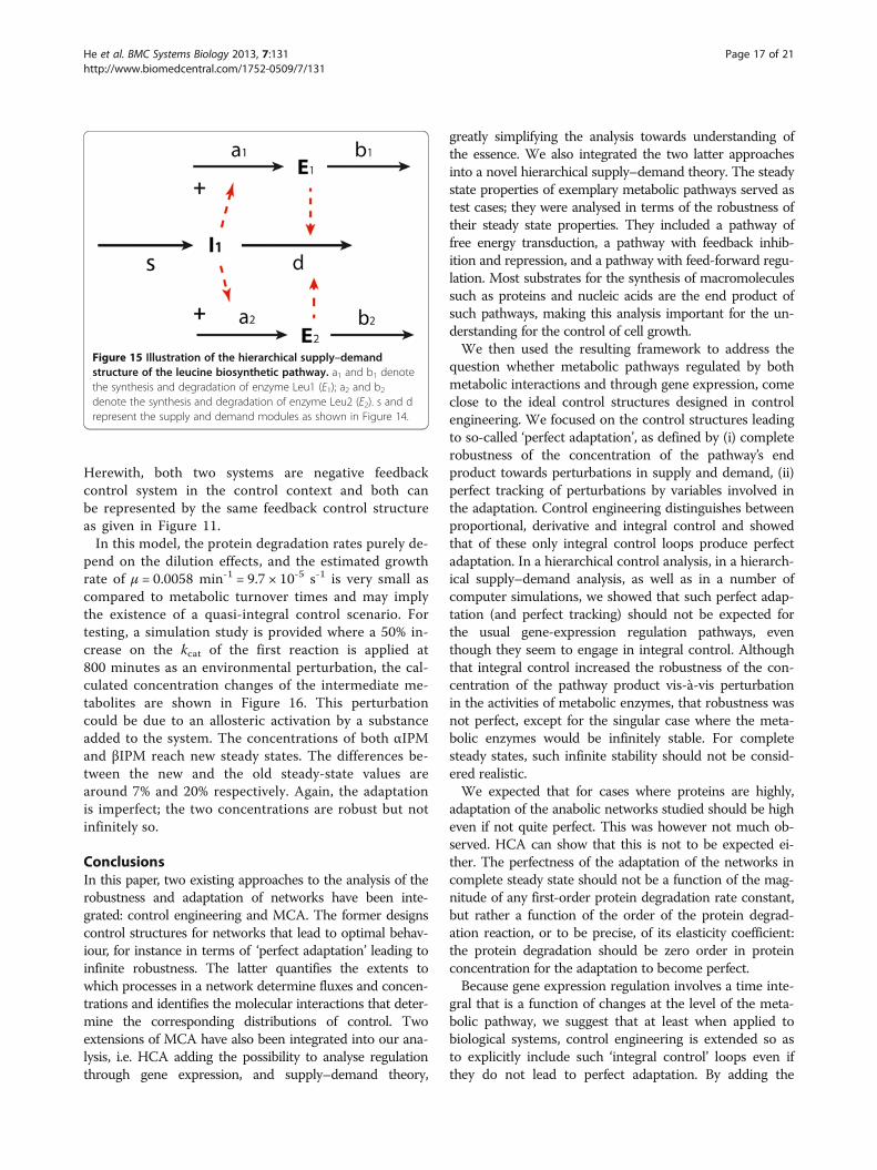
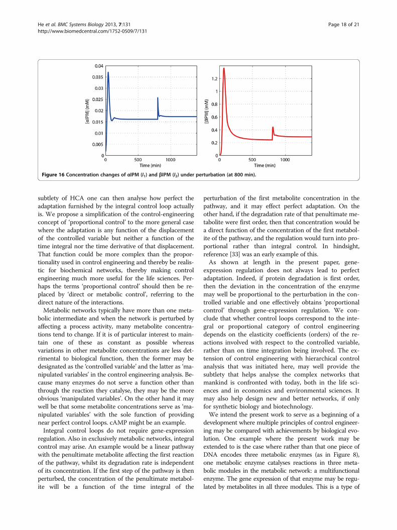
Herewith, both two systems are negative feedbackcontrol system in the control context and both canbe represented by the same feedback control structureas given in Figure 11.In this model, the protein degradation rates purely de-

pend on the dilution effects, and the estimated growthrate of μ = 0.0058 min-1 = 9.7 × 10-5 s-1 is very small ascompared to metabolic turnover times and may implythe existence of a quasi-integral control scenario. Fortesting, a simulation study is provided where a 50% in-crease on the kcat of the first reaction is applied at800 minutes as an environmental perturbation, the cal-culated concentration changes of the intermediate me-tabolites are shown in Figure 16. This perturbationcould be due to an allosteric activation by a substanceadded to the system. The concentrations of both αIPMand βIPM reach new steady states. The differences be-tween the new and the old steady-state values arearound 7% and 20% respectively. Again, the adaptationis imperfect; the two concentrations are robust but notinfinitely so.

ConclusionsIn this paper, two existing approaches to the analysis of therobustness and adaptation of networks have been inte-grated: control engineering and MCA. The former designscontrol structures for networks that lead to optimal behav-iour, for instance in terms of ‘perfect adaptation’ leading toinfinite robustness. The latter quantifies the extents towhich processes in a network determine fluxes and concen-trations and identifies the molecular interactions that deter-mine the corresponding distributions of control. Twoextensions of MCA have also been integrated into our ana-lysis, i.e. HCA adding the possibility to analyse regulationthrough gene expression, and supply–demand theory,

greatly simplifying the analysis towards understanding ofthe essence. We also integrated the two latter approachesinto a novel hierarchical supply–demand theory. The steadystate properties of exemplary metabolic pathways served astest cases; they were analysed in terms of the robustness oftheir steady state properties. They included a pathway offree energy transduction, a pathway with feedback inhib-ition and repression, and a pathway with feed-forward regu-lation. Most substrates for the synthesis of macromoleculessuch as proteins and nucleic acids are the end product ofsuch pathways, making this analysis important for the un-derstanding for the control of cell growth.We then used the resulting framework to address the

question whether metabolic pathways regulated by bothmetabolic interactions and through gene expression, comeclose to the ideal control structures designed in controlengineering. We focused on the control structures leadingto so-called ‘perfect adaptation’, as defined by (i) completerobustness of the concentration of the pathway’s endproduct towards perturbations in supply and demand, (ii)perfect tracking of perturbations by variables involved inthe adaptation. Control engineering distinguishes betweenproportional, derivative and integral control and showedthat of these only integral control loops produce perfectadaptation. In a hierarchical control analysis, in a hierarch-ical supply–demand analysis, as well as in a number ofcomputer simulations, we showed that such perfect adap-tation (and perfect tracking) should not be expected forthe usual gene-expression regulation pathways, eventhough they seem to engage in integral control. Althoughthat integral control increased the robustness of the con-centration of the pathway product vis-à-vis perturbationin the activities of metabolic enzymes, that robustness wasnot perfect, except for the singular case where the meta-bolic enzymes would be infinitely stable. For completesteady states, such infinite stability should not be consid-ered realistic.We expected that for cases where proteins are highly,

adaptation of the anabolic networks studied should be higheven if not quite perfect. This was however not much ob-served. HCA can show that this is not to be expected ei-ther. The perfectness of the adaptation of the networks incomplete steady state should not be a function of the mag-nitude of any first-order protein degradation rate constant,but rather a function of the order of the protein degrad-ation reaction, or to be precise, of its elasticity coefficient:the protein degradation should be zero order in proteinconcentration for the adaptation to become perfect.Because gene expression regulation involves a time inte-

gral that is a function of changes at the level of the meta-bolic pathway, we suggest that at least when applied tobiological systems, control engineering is extended so asto explicitly include such ‘integral control’ loops even ifthey do not lead to perfect adaptation. By adding the

Figure 15 Illustration of the hierarchical supply–demandstructure of the leucine biosynthetic pathway. a1 and b1 denotethe synthesis and degradation of enzyme Leu1 (E1); a2 and b2denote the synthesis and degradation of enzyme Leu2 (E2). s and drepresent the supply and demand modules as shown in Figure 14.


subtlety of HCA one can then analyse how perfect theadaptation furnished by the integral control loop actuallyis. We propose a simplification of the control-engineeringconcept of ‘proportional control’ to the more general casewhere the adaptation is any function of the displacementof the controlled variable but neither a function of thetime integral nor the time derivative of that displacement.That function could be more complex than the propor-tionality used in control engineering and thereby be realis-tic for biochemical networks, thereby making controlengineering much more useful for the life sciences. Per-haps the terms ‘proportional control’ should then be re-placed by ‘direct or metabolic control’, referring to thedirect nature of the interactions.Metabolic networks typically have more than one meta-

bolic intermediate and when the network is perturbed byaffecting a process activity, many metabolite concentra-tions tend to change. If it is of particular interest to main-tain one of these as constant as possible whereasvariations in other metabolite concentrations are less det-rimental to biological function, then the former may bedesignated as the ‘controlled variable’ and the latter as ‘ma-nipulated variables’ in the control engineering analysis. Be-cause many enzymes do not serve a function other thanthrough the reaction they catalyse, they may be the moreobvious ‘manipulated variables’. On the other hand it maywell be that some metabolite concentrations serve as ‘ma-nipulated variables’ with the sole function of providingnear perfect control loops. cAMP might be an example.Integral control loops do not require gene-expression

regulation. Also in exclusively metabolic networks, integralcontrol may arise. An example would be a linear pathwaywith the penultimate metabolite affecting the first reactionof the pathway, whilst its degradation rate is independentof its concentration. If the first step of the pathway is thenperturbed, the concentration of the penultimate metabol-ite will be a function of the time integral of the

perturbation of the first metabolite concentration in thepathway, and it may effect perfect adaptation. On theother hand, if the degradation rate of that penultimate me-tabolite were first order, then that concentration would bea direct function of the concentration of the first metabol-ite of the pathway, and the regulation would turn into pro-portional rather than integral control. In hindsight,reference [33] was an early example of this.As shown at length in the present paper, gene-

expression regulation does not always lead to perfectadaptation. Indeed, if protein degradation is first order,then the deviation in the concentration of the enzymemay well be proportional to the perturbation in the con-trolled variable and one effectively obtains ‘proportionalcontrol’ through gene-expression regulation. We con-clude that whether control loops correspond to the inte-gral or proportional category of control engineeringdepends on the elasticity coefficients (orders) of the re-actions involved with respect to the controlled variable,rather than on time integration being involved. The ex-tension of control engineering with hierarchical controlanalysis that was initiated here, may well provide thesubtlety that helps analyse the complex networks thatmankind is confronted with today, both in the life sci-ences and in economics and environmental sciences. Itmay also help design new and better networks, if onlyfor synthetic biology and biotechnology.We intend the present work to serve as a beginning of a

development where multiple principles of control engineer-ing may be compared with achievements by biological evo-lution. One example where the present work may beextended to is the case where rather than that one piece ofDNA encodes three metabolic enzymes (as in Figure 8),one metabolic enzyme catalyses reactions in three meta-bolic modules in the metabolic network: a multifunctionalenzyme. The gene expression of that enzyme may be regu-lated by metabolites in all three modules. This is a type of

Figure 16 Concentration changes of αIPM (I1) and βIPM (I2) under perturbation (at 800 min).


network structure that control engineering may come upwith as serving a function of coordination. And it will be ofinterest whether this type of network may serve a similarfunction in Biology.

AppendicesA. The initial-product moduleThe initial-product feed-forward regulation module givenin Figure 17 can be mathematically described by thefollowing differential equations:

_x1 tð Þ ¼ v0 tð Þ−E1 tð Þf 1 x1 tð Þ; p tð Þð Þ_x2 tð Þ ¼ E1 tð Þf 1 x1 tð Þ; p tð Þð Þ−E2 tð Þf 2 x2 tð Þ; x3 tð Þð Þ⋮ ⋮ ⋮

_xn tð Þ ¼ En−1 tð Þf n−1 xn−1 tð Þ; xn tð Þð Þ−En tð Þf n xn tð Þð Þ_E1 tð Þ ¼ g x1 tð Þð Þ−kEDE1 tð Þ

ð34ÞThe first reaction here is still assumed product insensitive

and other factors p can act on the enzyme. Different fromthe end-product module, the function g is assumed to bean increasing function of its argument. It has been demon-strated in [28] that if a constant steady-state regimen exists,the following simple relationship should be satisfied, with�E1 ¼ g �x1ð Þ=kED and g �x1ð Þ=kEDð Þ⋅f 1 �x1ð Þ ¼ v1 . Here, it isassumed the intermediate reactions of the metabolic path-ways do not ‘saturate’.

B. Calculation of global and local control coefficients in asupply–demand systemAccording to the summation and connectivity laws, for asupply–demand system, we have

CJd þ CJ

s ¼ 1

Cxnd þ Cxn

s ¼ 0

CJd⋅ε

dxn þ CJ

s⋅εsxn ¼ 0

Cxnd ⋅ε

dxn þ Cxn

s ⋅εsxn ¼ −1

By solving the above four equations, the ‘global’ con-centration and flux control coefficients with respect tothe supply and demand steps can be derived as

Cxns ¼ 1

εdxn−εsxn

; Cxnd ¼ −1

εdxn−εsxn

CJs ¼ −εdxn

εsxn−εdxn

; CJd ¼ εsxn

εsxn−εdxn

The expressions of the ‘local’ flux control coefficientsgiven in (5) can be obtained by solving the followingsummation and connectivity laws with respect to thelocal linear pathway within the supply module as givenin Figure 3.

cJ11 þ cJ12 þ⋯þ cJ1n−1 ¼ 1

cJ11 εv1x2 þ cJ12 ε

v2x2 ¼ 0

⋮cJ1n−2ε

vn−2xn−1 þ cJ1n−1ε

vn−1xn−1 ¼ 0

C. Steady state analysis of the ATP metabolism exampleThe steady state values of ADP and E before the per-turbation are determined when d[ADP]/dt = 0 and dE/dt = 0:

Ess ¼ kd⋅ C− ADP½ �ss� ks⋅ ADP½ �ss

ADP½ �ss ¼ kb⋅Ess þ k0ka

8>><>>:

ð35Þ

and

k0 ¼ ka⋅ ADP½ �ss−kb⋅kd⋅ C− ADP½ �ss� ks⋅ ADP½ �ss

ð36Þ

It is assumed that cell function requires ADP concen-tration to be at a certain level (i.e. [ADP]ss) and that inthe absence of the perturbation; the cell has adjusted Ess

Figure 17 The initial-product module with gene-expression and metabolic regulation.


and the rate constant k0 (and perhaps kd and ks) to meetthis requirement. We assume that the cell will do thisalso at different values of kb. The implication is that ifdifferent values of kb are considered, ka is also differentas defined by (36).Considering a perturbation of kd from its steady state

value, one finds for the time dependence of the variationin the enzyme level:

δ _E ¼ ka⋅ δ ADP½ �− kb⋅ δE ð37Þand for the time dependence of the variation in the levelof ADP:

δ ADP½ �:

¼ − ks⋅ Ess þ kdð Þ⋅ δ ADP½ �− ks⋅ ADP½ �ss⋅ δEþ C− ADP½ �ss�

⋅ δkdð38Þ

By integrating the time dependence of the change inenzyme level δE in (37) into (38) one finds (18). By sub-stituting the steady state condition of Ess in (35),

δ ADP½ �:

¼ −kd⋅C ⋅ δ ln ADP½ �− ks⋅ ADP½ �ss⋅ δEþ C− ADP½ �ss�

⋅ kd⋅ δ lnkd ð39ÞFor that change in ADP level to be time independent,

the integrand in the integral control term should equalzero around steady state, so that:

δE ¼ kakb⋅δ ADP½ � ð40Þ

By using this expression to eliminate the change in en-zyme level from (39) for the time dependence of thechange in ADP level and set the latter to zero, the ro-bustness coefficient in (21) can be obtained. Similarly, byusing (40) to eliminate the change in ADP level from(39), the control of enzyme level (19) can be obtained.

Competing interestsThe authors declare that they have no competing interests.

Authors’ contributionsFH and HVW jointly discussed and developed the main ideas of paper, and bothauthors wrote the manuscript. FH developed the hierarchical supply–demandtheory, proposed the control engineering analysis of the regulatory systems, andimplemented the simulation studies. HVW provided the MCA and HCA analysis,developed the first ATP metabolism example, identified the three terms incontrol analysis, and interpreted the results biochemically. VF contributed to thekinetic analysis of the end-product and initial-product modules. All authors readand approved the final manuscript and HVW rewrote the final version.

AcknowledgementsThis study was supported by the Netherlands Organization for ScientificResearch NWO through the MOSES-SysMO grant, as well as by the BBSRC(BRIC-BBSRC)/EPSRC’s funding of the Manchester Centre for Integrative SystemsBiology (DTC, BB/F003528/1, BB/C008219/1), BBSRC’s MOSES-SysMO project(DTC, BB/F003528/1), various other BBSRC projects (BB/G530225/1, BB/I004696/1,BB/I017186/1, BB/I00470X/1, BB/I004688/1, BB/J500422/1, BB/J003883/1, BB/J020060/1), and the EU-FP7 projects SYNPOL, EC-MOAN, UNICELLSYS, ITFoM,and BioSim. FH is partially supported by EPSRC and the European Research

Council (ERC) Advanced Investigator Grant. We thank an anonymous reviewerfor suggestions for improvements and additions that we took on board.

Author details1The Manchester Centre for Integrative Systems Biology, ManchesterInterdisciplinary Biocentre, University of Manchester, Manchester M1 7DN, UK.2Unité Mathématique, Informatique et Génomes, Institut National RechercheAgronomique, UR1077, F-78350 Jouy-en-Josas, France. 3Department ofAutomatic Control and Systems Engineering, The University of Sheffield,Sheffield S1 3JD, UK. 4Department of Synthetic Systems Biology and NuclearOrganization, Swammerdam Institute for Life Sciences, University ofAmsterdam, Science Park 904, NL-1098 XH Amsterdam, The Netherlands.5Department of Molecular Cell Physiology, Faculty of Earth and Life Sciences,VU University Amsterdam, De Boelelaan 1085, NL-1081 HV Amsterdam, TheNetherlands.

Received: 8 July 2013 Accepted: 12 November 2013Published: 21 November 2013

References1. Rossell S, Van Der Weijden CC, Lindenbergh A, van Tuijl A, Francke C, Bakker BM,

Westerhoff HV: Unraveling the complexity of flux regulation: a new methoddemonstrated for nutrient starvation in Saccharomyces cerevisiae. Proc NatlAcad Sci 2006, 103:2166–2171.

2. Ter Kuile BH, Westerhoff HV: Transcriptome meets metabolome: hierarchicaland metabolic regulation of the glycolytic pathway. FEBS Letters 2001,500(3):169–171.

3. Gerosa L, Sauer U: Regulation and control of metabolic fluxes inmicrobes. Curr Opin Microbiol 2011, 22(4):566–575.

4. Holzer H, Duntze W: Metabolic regulation by chemical modification ofenzymes. Annu Rew Biochem 1971, 40:345–374.

5. Bruggeman FJ, de Haan J, Hardin H, Bouwman J, Rossell S, van Eunen K,Bakker BM, Westerhoff HV: Time-dependent hierarchical regulation analysis:deciphering cellular adaptation. IEE Syst Biol 2006, 153(5):318–322.

6. Bruggeman FJ, Snoep JL, Westerhoff HV: Control, responses andmodularity of cellular regulatory networks: a control analysisperspective. IEE Syst Biol 2008, 2(6):397–410.

7. Feist AM, Herrgard MJ, Thiele I, Reed JL, Palsson BO: Reconstruction ofbiochemical networks in microbial organisms. Nat Rev Microbiol 2009,7(2):129–143.

8. McCloskey D, Palsson BO, Feist AM: Basic and applied uses of genome-scalemetabolic network reconstructions of Escherichia coli. Mol Syst Biol2013, 9:661.

9. Fell DA: Understanding the control of metabolism. London and Miami:Portland Press; 1997.

10. Kacser H, Burns JA: The control of flux. Symp Soc Exp Biol 1973, 27:65–104.11. Hofmeyr JH: Metabolic regulation: a control analytic perspective.

J Bioenerg Biomembr 1995, 27(5):479–490.12. Hofmeyr JH, Cornish-Bowden A: Quantitative assessment of regulation in

metabolic systems. Eur J Biochem 1991, 200:223–236.13. Hofmeyr JH, Cornish-Bowden A: Regulating the cellular economy of

supply and demand. FEBS Letters 2000, 476:47–51.14. Kahn D, Westerhoff HV: Control theory of regulatory cascades. J Theor Biol

1991, 153(2):255–285.15. Snoep JL, van der Weijden CC, Andersen HW, Westerhoff HV, Jensen PR:

DNA supercoiling in Escherichia coli is under tight and subtlehomeostatic control, involving gene-expression and metabolicregulation of both topoisomerase I and DNA gyrase. Eur J Biochem 2002,269:1662–1669.

16. Daran-Lapujade P, Rossell S, van Gulik WM, Luttik MA, de Groot MJ, Slijper M,Heck AJ, Daran JM, de Winde JH, Westerhoff HV, Pronk JT, Bakker BM: The fluxthrough glycolytic enzymes in Saccharomyces cerevisiae are predominantlyregulated at posttranscriptional levels. Proc Natl Acad Sci USA 2007,104:15753–15758.

17. Nise NS: Control systems engineering. 4th edition. Hoboken, NJ, USA: JohnWiley & Sons Inc; 2004.

18. Csete ME, Doyle J: Reverse engineering of biological complexity.Science 2002, 295:1664–1669.

19. Yi TM, Huang Y, Simon MI, Doyle J: Robust perfect adaptation in bacterialchemotaxis through integral feedback control. Proc Natl Acad Sci USA2000, 97:4649–4653.


20. El-Samad H, Goff JP, Khammash M: Calcium homeostasis and parturienthypocalcemia: an integral feedback perspective. J Theor Biol 2002,214:17–29.

21. Ni XY, Drengstig T, Ruoff P: The control of controller: molecularmechanisms for robust perfect adaptation and temperaturecompensation. Biophysical Journal 2009, 97:1244–1253.

22. Muzzey D, Gomez-Uribe CA, Mettetal JT, van Oudenaarden A: A systems-levelanalysis of perfect adaptation in yeast osmoregulation. Cell 2009,138(1):160–171.

23. Cloutier M, Wellstead P: The control systems structures of energymetabolism. J. R. Soc. Interface 2010, 7:651–665. 2010.

24. Tyson JJ, Chen KC, Novak B: Sniffers, buzzers, toggles and blinkers:dynamics of regulatory and signaling pathways in the cell. Curr Opin CellBiol 2003, 15:221–231.

25. Kacser H, Acerenza L: A universal method for achieving increases inmetabolite production. Eur J Biochem 1993, 216(2):361–367.

26. Fell DA, Thomas S: Physiological control of metabolic flux: therequirement for multisite modulation. Biochem J 1995, 311:35–39.

27. Adamczyk M, Westerhoff HV: Engineering of self-sustaining systems:substituting the yeast glucose transporter plus hexokinase for theLactococcus lactis phosphotransferase system in a Lactococcus lactisnetwork in silico. Biotech J 2012, 7(7):877–883.

28. Goelzer A, Briki FB, Marin-Verstraete I, Noirot P, Bessieres P, Aymerich S,Fromion V: Reconstruction and analysis of the genetic and metabolicregulatory networks of the central metabolism of Bacillus subtilis.BMC Systems Biology 2008, 2:20.

29. Gerhart JC, Pardee AB: The enzymology of control by feedback inhibition.J Biol Chem 1962, 237:891–896.

30. Shen-Orr SS, Milo R, Mangan S, Alon U: Network motifs in thetranscriptional regulation network of Escherichia coli. Nature Genet 2002,31:64–68.

31. Berg JM, Tymoczko JL, Stryer L: Biochemistry. 5th edition. New York: W HFreeman; 2002.

32. Westerhoff HV, Van Dam K: Thermodynamics and control of biologicalfree-energy transduction. Amsterdam: Elsevier; 1987.

33. Teusink B, Westerhoff HV: ‘Slave’ metabolites and enzymes. A rapid wayof delineating metabolic control. Eur J Biochem 2000, 267:1889–1893.

34. Schuster S, Kahn D, Westerhoff HV: Modular analysis of the control ofcomplex metabolic pathways. Biophys Chem 1993, 48(1):1–17.

35. Westerhoff HV, Koster JG, Van Workum M, Rudd KE: On the control of geneexpression. In Control of metabolic processes. Edited by Cornish-Bowden A.New York: Plenum; 1990:399–412.

36. Quinton-Tulloch MJ, Bruggeman FJ, Snoep JL, Westerhoff HV: Trade-off ofdynamic fragility but not of robustness in metabolic pathways in silico.FEBs Journal 2013, 280:160–173.

37. Roostalu J, Joers A, Luidalepp H, Kaldalu N, Tenson T: Cell division inEscherichia coli cultures monitored at single cell resolution.BMC Microbiology 2008, 8:68.

38. Vieira-Silva S, Rocha EPC: The systemic imprint of growth and its uses inecological (meta)genomics. PLoS Genet 2010, 6(1):e1000808.

39. Chin CS, Chubukov V, Jolly ER, DeRisi J, Li H: Dynamics and designprinciples of a basic regulatory architecture controlling metabolicpathways. PLoS Biol 2008, 6(6):1343–1356.

doi:10.1186/1752-0509-7-131Cite this article as: He et al.: (Im)Perfect robustness and adaptation ofmetabolic networks subject to metabolic and gene-expressionregulation: marrying control engineering with metabolic controlanalysis. BMC Systems Biology 2013 7:131. Submit your next manuscript to BioMed Central

and take full advantage of:

• Convenient online submission

• Thorough peer review

• No space constraints or color figure charges

• Immediate publication on acceptance

• Inclusion in PubMed, CAS, Scopus and Google Scholar

• Research which is freely available for redistribution

Submit your manuscript at www.biomedcentral.com/submit


(im)perfect robustness and adaptation of metabolic networks subject to metabolic and gene-expression...

Documents