Improved Estimation of the Covariance Matrix of Stock Returns

With an Application to Portfolio Selection

Olivier Ledoit

Anderson Graduate School of Management

University of California Los Angeles

and

Equities Division

Credit Suisse First Boston

Michael Wolf ∗

Dept. of Economics and Business

Universitat Pompeu Fabra

September 2002

Abstract

This paper proposes to estimate the covariance matrix of stock returns by an optimally

weighted average of two existing estimators: the sample covariance matrix and single-index

covariance matrix. This method is generally known as shrinkage, and it is standard in

decision theory and in empirical Bayesian statistics. Our shrinkage estimator can be seen

as a way to account for extra-market covariance without having to specify an arbitrary

multi-factor structure. For NYSE and AMEX stock returns from 1972 to 1995, it can

be used to select portfolios with significantly lower out-of-sample variance than a set of

existing estimators, including multi-factor models.

JEL CLASSIFICATION NOS: C13, C51, C61, G11, G15.

KEY WORDS: Covariance matrix estimation; Factor models; Portfolio selection; Shrinkage

method.

∗Michael Wolf, Dept. of Economics and Business, Universitat Pompeu Fabra, Ramon Trias Fargas 25–27,

E-08005 Barcelona, Spain; Phone: +34-93-542-2552, Fax: +34-93-542-1746, E-mail: michael.wolf@econ.upf.es.

We wish to thank Andrew Lo, John Heaton, Bin Zhou, Timothy Crack, Bruce Lehmann, Richard Michaud,

Richard Roll, Pedro Santa-Clara, and Jay Shanken for their feedback. Also, the paper has benefited from seminar

participants at MIT, the NBER, UCLA, Washington University in Saint Louis, Yale, Chicago, Wharton, UBC,

Pompeu Fabra, and Universitat Dortmund. All remaining errors are our own.

Research of the second author supported by DGES grant BEC2001-1270.

1

1 Introduction

The objective of this paper is to estimate the covariance matrix of stock returns. This is a

fundamental question in empirical Finance with implications for portfolio selection and for

tests of asset pricing models such as the CAPM.

The traditional estimator — the sample covariance matrix — is seldom used because it

imposes too little structure. When the number of stocks N is of the same order of magnitude

as the number of historical returns per stock T , the total number of parameters to estimate

is of the same order as the total size of the data set, which is clearly problematic. When N

is larger than T , the sample covariance matrix is always singular, even if the true covariance

matrix is known to be non-singular.1

These severe problems may come as a surprise, since the sample covariance matrix has

appealing properties, such as being maximum likelihood under normality. But this is to forget

what maximum likelihood means. It means the most likely parameter values given the data. In

other words: let the data speak (and only the data). This is a sound principle, provided that

there is enough data to trust the data. Indeed, maximum likelihood is justified asymptotically

as the number of observations per variable goes to infinity. It is a general drawback of maximum

likelihood that it can perform poorly in small sample. For the covariance matrix, small sample

problems occur unless T is at least one order of magnitude larger than N .

The cure is to impose some structure on the estimator. Ideally, the particular form of

the structure should be dictated by the problem at hand. In the case of stock returns, a

low-dimensional factor structure seems natural. But this leaves two very important questions:

How much structure should we impose? And what factors should we use?

To address these questions properly, we have to be more specific about how we impose

a low-dimensional factor structure. One possible way is to specify a K-factor model with

uncorrelated residuals. Then K controls how much structure we impose: the fewer the factors,

the stronger the structure. The advantages of this approach are that it is quite familiar to

the Finance profession, and that the factors sometimes have economic interpretation. The

disadvantages are that there is no consensus on the identity of the factors — except for the

first one, which represents a market index —, and that there is no consensus on the number

of factors K either (Connor and Korajczyk, 1995). In other words, choosing between factor

models is very ad hoc. It does not mean that none of them works well, it means that we do not

know which one works well a priori. For example, if we are interested in selecting portfolios

with low out-of-sample variance, in any given data set there may exist a factor model that

performs well, but it may be a different one for every data set, and there is no way of telling

which one works well without looking out-of-sample, which is cheating. The art of choosing a

factor model adapted to a given data set without seeing its out-of-sample fit is just that: an

art.

1In typical applications, there can be over a thousand stocks to choose from, but rarely more than ten years

of monthly data, i.e., N = 1, 000 and T = 120.

2

This is why, in this paper, we study another way of imposing factor structure. It is to

take a weighted average of the sample covariance matrix with Sharpe’s (1963) single-index

model estimator. The weight α (between zero and one) assigned to the single-index model

controls how much structure we impose: the heavier the weight, the stronger the structure.

This is a well-known technique in Statistics called shrinkage dating back to Stein (1956): α is

called the shrinkage intensity, and the single-index model is our choice of shrinkage target. The

advantages are that there is strong consensus on the nature of the single factor (a market index),

and that there is a way of estimating the optimal shrinkage consistently. The estimation of α is

the technically challenging part of this paper. It provides a rigorous answer to the question of

how much structure we should impose. On any given data set, there will be a different optimal

shrinkage intensity, and our estimation technique will find it without having to look out-of-

sample. This takes the ad-hockery out of the task of imposing structure on the covariance

matrix of stock returns. It replaces the art of factor selection by a fully automatic procedure.

At this point, it is worth mentioning that the paper is solely concerned with the structure

of risk in the stock market, not with the structure of expected returns. Multi-factor models

of the covariance matrix can still be very useful if economic arguments tie them up to the

cross-section of expected returns, as in the Arbitrage Pricing Theory of Ross (1976). Any

discussion of the relationship between risk factors and expected returns is outside the scope

of the paper. There should be no ambiguity over whether we define “factors” in terms of the

mean vector or of the covariance matrix of stock returns: it is always the latter.

Muirhead (1987) reviews the large literature on shrinkage estimators of the covariance

matrix in finite-sample statistical decision theory. All these estimators suffer from at least two

severe drawbacks, either of which is enough to make them ill-suited to stock returns: (i) they

break down when N > T ; (ii) they do not exploit the a priori knowledge that stock returns

tend to be positively correlated to one another. Frost and Savarino (1986) show that the

solution to the second problem is to use a shrinkage target that incorporates a market factor,

but they ignore without justification the correlation between estimation error on the shrinkage

target and on the covariance matrix, and they are still exposed to the first problem. A main

contribution of our paper to the literature is to address the first problem through the definition

the optimal shrinkage intensity by minimizing a loss function that does not involve the inverse

of the covariance matrix. Moreover, the technique is so general that it is applicable to other

shrinkage targets as well.

A noteworthy innovation is that the optimal shrinkage intensity depends on the correlation

between estimation error on the sample covariance matrix and on the shrinkage target. Intu-

itively, if the two of them are positively (negatively) correlated, then the benefit of combining

the information that they contain is smaller (larger). The introduction of this correlation term

resolves a deep logical inconsistency in earlier empirical Bayesian literature, where the prior is

estimated from sample data, yet at the same time is assumed to be independent from sample

data.

We test the performance of our shrinkage estimator on stock returns data for portfolio

3

selection. Using NYSE and AMEX stocks from 1972 to 1995, we find that our estimator

yields portfolios with significantly lower out-of-sample variance than a set of well-established

competitors, including multi-factor models.

The remainder of the paper is organized as follows. Section 2 presents our shrinkage

estimator of the covariance matrix. Section 3 presents empirical evidence on its out-of-sample

performance for portfolio selection. Finally, Section 4 concludes. All figures and tables appear

at the end of the paper.

2 Shrinkage Estimator of the Covariance Matrix

This section presents the covariance matrix estimator that we recommend for stock returns.

2.1 Statistical Model

Let X denote an N×T matrix of T observations on a system of N random variables representing

T returns on a universe of N stocks.

Assumption 1 Stock returns are independent and identically distributed (iid) through time.

Even though actual stock returns do not verify Assumption 1, it is an acceptable first-cut

approximation. This means that we abstract from lead-lag effects (Lo and MacKinlay, 1990),

nonsynchronous trading (Shanken, 1987), and autoregressive conditional heteroskedasticity

(Bollerslev, Engle and Woooldridge, 1988). Note that most of the current estimators for the

covariance matrix of stock returns also use this assumption. Future research will be devoted

to relaxing it. It is, however, not clear that by introducing extra degrees of freedom in the

estimation process to account for dependence and conditional heteroskedasticity one will be

able to improve out-of-sample performance.

Assumption 2 The number of stocks N is fixed and finite, while the number of observations

T goes to infinity.

Assumption 3 Stock returns have finite fourth moment:

∀i, j, k, l = 1, . . . , n ∀t = 1, . . . , T E[|xitxjtxktxlt|] < ∞.

This is so that we can apply the Central Limit Theorem to sample variances and covariances.

Note that stock returns are not assumed to be normally distributed in this paper.

4

2.2 Sample Covariance Matrix

The sample mean vector m and the sample covariance matrix S are defined by:

m =1

TX1 (1)

S =1

TX

(I− 1

T11′

)X′ (2)

where 1 denotes a conformable vector of ones and I a conformable identity matrix.2 Equa-

tion (2) shows why the sample covariance matrix is not invertible when N ≥ T : the rank of

S is at most equal to the rank of the matrix I − 11′/T , which is T − 1. Therefore when the

dimension N exceeds T − 1, the sample covariance matrix is rank-deficient. Intuitively, the

data do not contain enough information to estimate the unrestricted covariance matrix.

2.3 Single-Index Covariance Matrix Estimator

Sharpe’s (1963) single-index model assumes that stock returns are generated by:

xit = αi + βix0t + εit

where residuals εit are uncorrelated to market returns x0t and to one another. Also, within

stocks the variance is constant, that is, V ar(εit) = δii. The covariance matrix implied by this

model is:

Φ = σ200ββ′ + ∆

where σ200 is the variance of market returns, β is the vector of slopes, and ∆ is the diagonal

matrix containing residual variances δii. Call φij the (i, j)-th entry of Φ.

This model can be estimated by running a regression of stock i’s returns on the market.

Call bi the slope estimate and dii the residual variance estimate. Then the single-index model

yields the following estimator for the covariance matrix of stock returns:

F = s200bb′ + D

where s200 is the sample variance of market returns, b is the vector of slope estimates, and D

is the diagonal matrix containing residual variance estimates dii. Call fij the (i, j)-th entry

of F. We need to make two technical assumptions.

Assumption 4 Φ 6= Σ

Assumption 5 The market portfolio has positive variance, that is, σ200 > 0.

The exact composition of the market portfolio is not as critical here as it is for the CAPM

(Roll, 1977). All we need is for x0t to explain a significant part of the variance of most stocks,

2Vectors (matrices) are denoted in lower (upper) case boldface.

5

and any broad-based market index would do. As a matter of fact, equal-weighted indices are

better at explaining stock market variance than value-weighted indices, yet another departure

from CAPM intuition. The assumption that residuals are uncorrelated to one another should

theoretically preclude that the portfolio which makes up the market contain any of the N stocks

in the sample. However, as long as the size of the portfolio is large, such a violation will have

a very small effect and is typically ignored in applications.

2.4 General Form of the Shrinkage Estimator

At one extreme, the single-index covariance matrix comes from a one-factor model, while at

the other extreme, the sample covariance matrix can be interpreted as an N -factor model

(each stock being a factor, there are no residuals). The intuition of the profession has always

been that the best model lies somewhere between these two extremes. For example, Rosenberg

(1974) stresses the importance of extra-market covariance, while Jobson and Korkie (1980)

document the poor performance of the sample covariance matrix. Until now, this intuition has

been expressed mostly through K-factor models with 1 < K < N .

If we abstract ourselves from the Finance context and look at the broader picture from a

statistician’s point of view, we see another way of capturing the same intuition. The key is

to recognize that the single-index model covariance matrix has a lot of bias coming from a

stringent and misspecified structural assumption, but little in the way of estimation error, and

that the opposite is true of the sample covariance matrix: it is unbiased (asymptotically) but

has a lot of estimation error. A fundamental principle of statistical decision theory is that there

exists an interior optimum in the trade-off between bias and estimation error. Since Stein’s

(1956) seminal work, we know that one way of attaining this optimal trade-off is simply to take

a properly weighted average of the biased and unbiased estimators. This is called shrinking

the unbiased estimator full of estimation error towards a fixed target represented by the biased

estimator. For example, Stein (1956) showed that shrinking sample means towards a constant

can, under certain circumstances, improve accuracy. Efron and Morris (1977) provide a general

introduction to shrinkage, and Jorion (1986) shows its importance in the context of portfolio

selection.

Here this well-established statistical method suggests taking a weighted average of the

single-index model covariance matrix and the sample covariance matrix. This is an alternative

way of capturing the intuition that led to the development of multi-factor models. The main

advantage of this alternative is that it does not require knowledge of the number and nature

of factors (beyond the obvious market factor).

2.5 Formula for the Optimal Shrinkage Intensity

The obvious problem in the application of our method is the selection of the shrinkage intensity.

This section discusses the optimal shrinkage intensity and its consistent estimation from the

data. Since N is fixed and T goes to infinity, S is consistent but F is not, therefore the optimal

6

shrinkage intensity vanishes asymptotically. As will be shown below, it is of the (expected)

order O(1/T ). To simplify the estimation, we therefore will focus on shrinkage intensities of

the form α = constant/T. The goal then becomes to first find the optimal constant and to

then estimate it consistently in order to arrive at a feasible shrinkage estimator.

We have to choose the objective according to which the shrinkage intensity is “optimal.”

All existing shrinkage estimators from finite-sample statistical decision theory and also Frost

and Savarino’s (1986) break down when N ≥ T because their loss functions involve the inverse

of the covariance matrix. Instead, we propose a loss that does not depend on this inverse. The

loss function is extremely intuitive: it is a quadratic measure of distance between the true and

the estimated covariance matrices based on the Frobenius norm.

Definition 1 The Frobenius norm of the N×N symmetric matrix Z with entries (zij)i,j=1,...,N

and eigenvalues (λi)i=1,...,N is defined by:

‖Z‖2 = Trace(Z2) =N∑

i=1

N∑

j=1

z2ij =

N∑

i=1

λ2i

By considering the Frobenius norm of the difference between the shrinkage estimator and the

true covariance matrix, we arrive at the following quadratic loss function:

L(α) = ‖αF + (1 − α)S−Σ‖2 ,

which gives rise to the risk function

R(α) = E(L(α)) =N∑

i=1

N∑

j=1

E(α fij + (1 − α) sij − σij)2

=N∑

i=1

N∑

j=1

Var (α fij + (1 − α) sij) + [E (α fij + (1 − α) sij − σij)]2

=N∑

i=1

N∑

j=1

α2Var(fij) + (1 − α)2Var(sij) + 2α(1 − α)Cov(fij, sij) + α2(φij − σij)2.

The goal now is to minimize the risk R(α) with respect to α. Calculating the first two deriva-

tives of R(α) yields after some basic algebra

R′(α) = 2N∑

i=1

N∑

j=1

αVar(fij) − (1 − α)Var(sij) + (1 − 2α)Cov(fij, sij) + α(φij − σij)2

R′′(α) = 2N∑

i=1

N∑

j=1

Var(fij − sij) + (φij − σij)2.

Setting R′(α) = 0 and solving for α∗ we get

α∗ =

∑Ni=1

∑Nj=1 Var(sij) − Cov(fij, sij)

∑Ni=1

∑Nj=1 Var(fij − sij) + (φij − σij)2

. (3)

Since R(α)′′ is positive everywhere, this solution is verified as a minimum of our risk function.

It is easy to see that α∗ = O(1/T ). Indeed, the following Theorem shows the first order

asymptotic behavior of the optimal shrinkage intensity α∗.

7

Theorem 1 Let π denote the sum of asymptotic variances of the entries of the sample covari-

ance matrix scaled by√

T : π =∑N

i=1

∑Nj=1 AsyVar

[√Tsij

]. Similarly, let ρ denote the sum of

asymptotic covariances of the entries of the single-index covariance matrix with the entries of

the sample covariance matrix scaled by√

T : ρ =∑N

i=1

∑Nj=1 AsyCov

[√Tfij,

√Tsij

]. Finally,

let γ measure the misspecification of the single-index model: γ =∑N

i=1

∑Nj=1(φij −σij)

2. Then

the optimal shrinkage α∗ satisfies:

α∗ =1

T

π − ρ

γ+ O

(1

T 2

). (4)

Proof of Theorem 1 Relation (3) implies that

Tα∗ =

∑Ni=1

∑Nj=1 Var(

√Tsij) − Cov(

√Tfij,

√Tsij)

∑Ni=1

∑Nj=1 Var(fij − sij) + (φij − σij)2

. (5)

By standard arguments, using the assumptions of iid data and finite fourth moments, it follows

that

N∑

i=1

N∑

j=1

Var(√

Tsij) → πN∑

i=1

N∑

j=1

Cov(√

Tfij,√

Tsij) → ρ andN∑

i=1

N∑

j=1

Var(fij − sij) = O

(1

T

).

(6)

Indeed, to show the first convergence, it is sufficient to focus on an arbitrary element

πij = AsyVar[√

Tsij]. Without loss of generality assume that E(xit) = E(xjt) = 0. We start

with the statistic

σij =1

T

T∑

t=1

xitxjt.

Note that xi1xj1, . . . , xiT xjT is an iid sequence with mean πij and finite variance %ij, say. The

standard CLT therefore implies that

√T (σij − σij) =⇒ N(0, %2

ij), (7)

where =⇒ denotes convergence in distribution. Let xi· = T−1∑T

t=1 xit and xj· = T−1∑T

t=1 xjt.

Then,

√T (σij − sij) =

√Txi·

1

T

T∑

t=1

(xjt − xj·) +√

Txj·

1

T

T∑

t=1

(xit − xi·) +√

Txi·xj·

=√

Txi·xj·.

By the standard CLT again,√

Txi· has a limiting normal distribution and is thus OP (1). On

the other hand, xj· converges to zero almost surely and is thus oP (1). Hence, it is easily seen

that√

T (σij − sij) = oP (1). By the convergence in distribution (7) and Slutzky’s theorem, it

follows that √T (sij − σij) =⇒ N(0, %ij).

Moreover, this implies that %ij = πij and that Var(√

Tsij) → πij. Since we focused on an

arbitrary element πij, the same argument can be used for the other elements as well. Combining

8

the individual convergences (noting that there are a finite and fixed number of them), we arrive

at∑N

i=1

∑Nj=1 Var(

√Tsij) → π.

The convergence∑N

i=1

∑Nj=1 Cov(

√Tfij,

√Tsij) → ρ is proved analogously.

Finally, a similar argument can be used to demonstrate that∑N

i=1

∑Nj=1 Var(

√T(fij − sij))

converges to a positive limit, which implies that∑N

i=1

∑Nj=1 Var(fij − sij) = O(1/T).

We thus have verified the claim (6). But (5) and (6) together imply (4) and this completes

the proof.

The theorem shows that within the class of shrinkage intensities {α = constant/T}, the

asymptotically optimal choice is given by constant = κ with κ = (π − ρ)/γ. The analysis

of the optimal constant κ indicates the following. The weight placed on the single-index

model increases in the error on the sample covariance matrix (through π) and decreases in the

misspecification of the single-index model (through γ). An alternative interpretation of this

solution is a geometric one: κTF +

(1 − κ

T

)S is (asymptotically) the orthogonal projection of

the true covariance matrix Σ onto the line joining single-index model and sample covariance

matrices (see Figure 1).

Note also the appearance of the term ρ that measures the covariance between the estimation

errors of S and F and was not present in the work of Frost and Savarino (1986). It is easier

to understand within the empirical Bayesian interpretation of our shrinkage estimator: we

can say that we have a prior based on the single-index model which we combine with sample

information. Estimating the prior F from the same data set as S violates the pure Bayesian

principle that prior and sample information should be independent. This is typical of the

empirical Bayesian approach. Yet this violation is often ignored, and there is an “art” to

choosing the prior so that the violation is not too damaging. We get rid of the need for such

artistry by explicitly taking into account the correlation between prior and sample information

through ρ.

Finally, the reader can verify that Theorem 1 is of general nature: nowhere did we use the

fact that F is a single-index model estimator. Equation (4) stays the same as long as F is an

asymptotically biased estimator of the covariance matrix and satisfies a set of weak regularity

conditions.

2.6 A Consistent Estimator of the Optimal Shrinkage Constant

Note that κTF +

(1 − κ

T

)S is not a bona fide estimator because κ depends on unobservables.

Therefore, we need to find a consistent estimator for κ = (π − ρ)/γ. We can decompose π

into π =∑N

i=1

∑Nj=1 πij where πij = AsyVar

[√Tsij

], ρ into ρ =

∑Ni=1

∑Nj=1 ρij where ρij =

AsyCov[√

Tfij,√

Tsij], and γ into γ =

∑Ni=1

∑Nj=1 γij where ρij = (φij − σij)

2. Standard

asymptotic theory provides consistent estimators for πij , ρij and γij.

9

Lemma 1 A consistent estimator for πij is given by:

pij =1

T

T∑

t=1

{(xit − mi)(xjt − mj) − sij}2 .

Proof of Lemma 1 pij is the usual estimator for the asymptotic variance of sij. It converges

in probability to Var[(xi1 − µi)(xj1 − µj)], which is equal to πij.

Let m0 denote the sample mean of market returns and si0 the sample covariance of stock i’s

returns with the market.

Lemma 2 On the diagonal a consistent estimator of ρii is given by rii = pii, and for i 6= j a

consistent estimator of ρij is given by rij = 1T

∑Tt=1 rijt where:

rijt =sj0s00(xit − mi) + si0s00(xjt − mj) − si0sj0(x0t − m0)

s200

(x0t − m0)(xit − mi)(xjt − mj)

− fijsij. (8)

Proof of Lemma 2 On the diagonal fii = sii, therefore ρii = πii can be consistently esti-

mated by rii = pii. When i 6= j we have: fij = bibjs00 = si0sj0/s00, therefore the delta method

yields:

ρij = AsyCov

[√T

si0sj0s00

,√

Tsij

]

=σj0

σ00

AsyCov[√

Tsi0,√

Tsij]+

σi0

σ00

AsyCov[√

Tsj0,√

Tsij]

− σi0σj0

σ200

AsyCov[√

Ts00,√

Tsij]. (9)

A consistent estimator for σk0 where k = 0, k = i or k = j is sk0. The usual estimator for

AsyCov[√

Tsk0,√

Tsij]

where k = 0, k = i or k = j is:

1

T

T∑

t=1

{(xkt − mk)(x0t − m0) − sk0

}{(xit − mi)(xjt − mj) − sij

}.

Plugging these estimators into Equation (9) and rearranging yields Equation (8).

Lemma 3 A consistent estimator for γij = (φij − σij)2 is its sample counterpart cij =

(fij − sij)2.

Proof of Lemma 3 This is because fij and sij are consistent estimators for φij and σij ,

respectively.

Now it is easy to construct an estimator for the optimal shrinkage constant.

Theorem 2 k = (p − r)/c is a consistent estimator for the optimal shrinkage constant κ =

(π − ρ)/γ.

10

Proof of Theorem 2 Under Assumption 4 (γ > 0), combining the results of Lemmata 1–3

proves the theorem.

Using this notation, the shrinkage estimator for the covariance matrix of stock returns that we

recommend is:3

S =k

TF +

(1 − k

T

)S (10)

Different shrinkage targets would lend themselves just as well to a corresponding estimation

of π, ρ and γ. The formula for r would need to be readjusted on a case-by-case basis, but the

formulas for p and c would not change.

3 Empirical Results

We present empirical evidence on the performance of the shrinkage estimator defined in the

last section. We compare it to existing estimators in terms of its ability to select portfolios of

stocks with low out-of-sample variance.

3.1 Portfolio Selection

Consider a universe of N stocks whose returns are distributed with mean vector µ and covari-

ance matrix Σ. Markowitz (1952) defines the problem of portfolio selection as:

minw

w′Σw

subject to

∣∣∣∣∣w′1 = 1

w′µ = q

(11)

where 1 denotes a conformable vector of ones and q is the expected rate of return that is

required on the portfolio. The well-known solution is:

w =C − qB

AC − B2Σ−11 +

qA − B

AC − B2Σ−1µ (12)

where A = 1′Σ−11, B = 1′Σ−1µ and C = µ′Σ−1µ

Equation (12) shows that optimal portfolio weights depend on the inverse of the covariance

matrix. This sometimes causes difficulty if the covariance matrix estimator is not invertible

or if it is numerically ill-conditioned, which means that inverting it amplifies estimation error

tremendously (Michaud, 1989). The shrinkage estimator S is the weighted average of two

positive semi-definite matrices, one of which (F) is invertible, therefore it is invertible. Also,

it inherits the good-conditioning of the single-index model estimator, not the ill-conditioning

of the sample covariance matrix.

In practice, the covariance matrix is estimated from historical data available up to a given

date, optimal portfolio weights are computed from this estimate, then the portfolio is formed

3Matlab code implementing this estimator can be downloaded from www.ledoit.net

11

on that date and held until the next rebalancing occurs. The performance of a covariance

matrix estimator is measured by the variance of this optimal portfolio after it is formed. It

is a measure of out-of-sample performance, or of predictive ability. An estimator that overfits

in-sample data can turn out to work very poorly for portfolio selection, which is why imposing

some structure is beneficial.

The other input into portfolio selection is the vector of expected returns. It is sometimes

argued that estimating the covariance matrix well is less important than estimating the ex-

pected returns well. We believe that this view is profoundly misguided. First, the essence

of mean-variance analysis is that there is a trade-off between risk and return, therefore any

reduction in risk translates into an increase in expected returns. Second, having a good esti-

mator of the covariance matrix helps us estimate more precisely the excess return associated

with, for example, beta, size, or book-to-market by constructing portfolios that load on these

characteristics and have low variance (this is related to the efficiency gain in running GLS

cross-sectional regressions of stock returns on these characteristics). Third, it is not the role

of just the statistician to determine expected returns, it is also the role of the economist, and

of the portfolio manager who is paid to generate valuable private information about future

stock price movements; whereas only statistics can generate information about the covariance

matrix. This justifies why it is perfectly legitimate to concentrate on the covariance matrix

alone without worrying about expected returns, as we do here.

3.2 Data

Stock returns were extracted from the Center for Research in Security Prices (CRSP) monthly

database. The same procedure is repeated for every year from t = 1972 to t = 1994. We use

data from August of year t − 10 to July of year t to estimate the covariance matrix of stock

returns.4 Then on the first trading day in August of year t we build a portfolio with minimum

variance (according to this covariance matrix estimate) under certain constraints. We hold this

portfolio until the last trading day in July of year t+1, at which time we liquidate it and start

the process all over again. Thus, the in-sample period goes from August of year t− 10 to July

of year t, and the out-of-sample period goes from August of year t to July of year t + 1. The

main quantity of interest is the out-of-sample standard deviation of this investment strategy

over the 23-year period from August 1972 to July 1995. This is a predictive test, in the sense

that our investment strategy does not require any hindsight.

In August of year t, we consider the universe of common stocks traded on the New York

Stock Exchange (NYSE) and the American Stock Exchange (AMEX) with valid CRSP returns

for the last 120 months and valid Standard Industrial Classification (SIC) codes. The resulting

number of stocks varies across years between N = 909 and N = 1, 314.

We consider two minimum variance portfolios: the global minimum variance portfolio, and

the portfolio with minimum variance under the constraint of having 20% expected return. In

4We rebalance every August because the earliest AMEX stock returns available from CRSP are in August

1962.

12

both cases short sales are allowed, and no additional restriction is imposed (except that weights

sum up to one). It is common practice in the investment community to impose client-specific

constraints on portfolio weights or to minimize active risk with respect to an exogenously

specified benchmark, but we abstract from that in order to have a “maximum stress” test of

the performance of the covariance matrix estimator. For expected returns, we just take the

average realized return over the last 10 years. This may or may not be a good predictor of

future expected returns, but our goal is not to predict expected returns: it is only to show

what kind of reduction in out-of-sample variance our method yields under a fairly reasonable

linear constraint.

3.3 Competing Estimators

Apart from our shrinkage estimator, we consider the following covariance matrix estimators

proposed in the literature.

Identity The simplest model is to assume that the covariance matrix is a scalar multiple of

the identity matrix. This is the assumption implicit in running an Ordinary Least Squares

(OLS) cross-sectional regression of stock returns on stock characteristics, as Fama and MacBeth

(1973) and their successors do. Interestingly, it yields the same weights for the minimum

variance portfolios as a two-parameter model where all variances are equal to one another and

all covariances are equal to one another. This two-parameter model is discussed by Jobson

and Korkie (1980) and by Frost and Savarino (1986).

Constant Correlation Elton and Gruber (1973) recommend a model where every pair of

stocks has the same correlation coefficient. Thus, there are N + 1 parameters to estimate: the

N individual variances, and the constant correlation coefficient.

Pseudo-Inverse It is impossible to use the sample covariance matrix directly for portfolio

selection when the number of stocks N exceeds the number of historical returns T , which is the

case here. The problem is that we need the inverse of the sample covariance matrix, and it does

not exist. One possible trick to get around this problem is to use the pseudo-inverse, also called

generalized inverse or Moore-Penrose inverse. Replacing the inverse of the sample covariance

matrix by the pseudo-inverse into Equation (12) yields well-defined portfolio weights.

Market Model This is the single-index covariance matrix of Sharpe (1963), which is defined

in Section 2.3.

13

Industry Factors This refinement of the single-index model assumes that market residuals

are generated by industry factors:

xit = αi + βix0t +K∑

k=1

cikzkt + εit (13)

where K is the number of industry factors, cik is a dummy variable equal to one if stock

i belongs to industry category k, zkt is the return to the k-th industry factor in period t,

and εkt denotes residuals that are uncorrelated to the market, to industry factors, and to

each other. Every stock is assigned to one of the 48 industries defined by Fama and French

(1997). This high number of factors is similar to the one used by the company BARRA to

produce commercial multi-factor estimates of the covariance matrix (Kahn, 1994).5 Industry

factor returns are defined as the return to an equally-weighted portfolio of the stocks from this

industry in our sample.

Principal Components An alternative approach to multi-factor models is to extract the

factors from the sample covariance matrix itself using a statistical method such as principal

components. Some investment consultants such as Advanced Portfolio Technologies success-

fully use a refined version of this approach (Bender and Blin, 1997). Since principal components

are chosen solely for their ability to explain risk, fewer factors are necessary, but they do not

have any direct economic interpretation.6 A sophisticated test by Connor and Korajczyk

(1993) finds between four and seven factors for the NYSE and AMEX over 1967–1991, which

is in the same range as the original test by Roll and Ross (1980). The number of factors that

we use here is five.

Shrinkage Towards Identity A related shrinkage estimator of Ledoit and Wolf (2000)

uses a scalar multiple of the identity matrix as shrinkage target; note that their estimator,

under a different asymptotic framework, is suggested for general situations where no “natural”

shrinking target exists. This seems suboptimal for stock returns, since stock returns have

mainly positive covariances. Hence, it appears beneficial to use a shrinkage target which

incorporates this knowledge, such as the single-index covariance matrix. Nevertheless, we

include this estimator.

Shrinkage Towards Market This is the estimator S defined in (10).

3.4 Out-of-Sample Standard Deviations

For every one of the eight estimators described in the previous subsection, we compute the

out-of-sample (annualized) standard deviation of the minimum variance portfolios as per Sec-

tion 3.2. The results are in Table 1.5In addition, BARRA use proprietary methods, including other factors that are not industry-based, therefore

this is not a test of their performance.6Except for the first factor, which is highly correlated with the market index.

14

We can see that naive diversification (one dollar in every stock) performs the worst, while

the shrinkage estimator developed above performs the best; somewhat surprisingly, maybe,

shrinking towards the identity is second best and also beats all of the previously suggested

methods. The t-statistics of whether S yields portfolios with lower variance than its seven

competitors range from 2.73 (against the other shrinkage estimator) to 7.39 (against the con-

stant correlation model).

To assess economic significance, the rule of thumb is that a decrease of two basis points

in standard deviation corresponds to an increase of one basis points in expected returns,

using standard numbers for the risk-return tradeoff.7 For example, gains over the two multi-

factor models are 43 and 94 basis points respectively in terms of average returns for the

constrained portfolio. By this metric, improvement over the two multi-factor models and the

shrinkage towards the identity is reasonable. Improvement over the other estimators, including

the sample covariance matrix and the single-index model (the ones which we are combining

together), is large.

3.5 Weight Distribution

We also report descriptors of the weights of the global minimum variance portfolio: turnover,

short interest, lowest and highest weight. When a stock has missing out-of-sample observations

we assume that it earns the riskfree rate. Thus, it is important to report the cash position,

defined as the total amount invested in stocks with missing observations. These weight de-

scriptors are in Table 2.

If we wanted to do portfolio selection in practice, all these minimum variance portfolios

would have too much of a short interest to be really attractive. But absolutely no effort was

made to control for this characteristic, therefore there is considerable room for improving it

without substantially degrading the performance reported in Table 1. In our view, Table 2 in-

dicates that the weight distribution generated by the shrinkage estimator is acceptable overall.

The cash position due to missing out-of-sample observations is always very small, therefore

the standard deviations in Table 1 do indeed correspond to portfolios almost fully invested in

equities. Otherwise, it would be easy to get low risk simply by holding cash.

3.6 Shrinkage Intensity

Figure 2 shows how the estimate of the optimal shrinkage intensity evolves through the 23 years

in our sample.

It is always between zero and one, which is what we would expect. It is remarkably stable

through time. In particular, this implies that there is very little estimation error, as predicted

by Theorem 2. It is fairly high: around 80%. This means that there is four times as much

estimation error in the sample covariance matrix as there is bias in the single-index model.

7Specifically: 8.5% market risk premium and 17% market standard deviation (annualized).

15

While k/T is an asymptotically negligible correction, we see that in practice it can make a big

difference.

In spite of the large number of stocks, the computations are remarkably fast. Using a

desktop personal computer and a Matlab program, it took us about three seconds to compute

the optimal shrinkage intensity, the covariance matrix estimator S, and the minimum variance

portfolio weights for N = 1, 000 stocks.

The term r in the formula for the optimal shrinkage intensity, which is one of the major

innovations of this paper, turns out to be critical in practice. If we had omitted it, all the

shrinkage intensities would have been well above one and thus meaningless.

4 Conclusion

We have developed a flexible method for imposing some structure into a large-dimensional

estimation problem, namely the problem of estimating the covariance matrix of a large number

of stock returns. The crux of the method is to shrink the unbiased but very variable sample

covariance matrix towards the biased but less variable single-index model covariance matrix and

to thereby obtain a more efficient estimator. In addition, the resulting estimator is invertible

and well-conditioned, which is of crucial importance in case one needs to estimate the inverse

of the true covariance matrix.

The practical problem in applying our method is to to determine the shrinkage intensity,

that is, the amount of shrinkage of the sample covariance matrix towards the single-index

model covariance matrix. The problem was solved by first demonstrating that the optimal

shrinking intensity, to second order, behaves like a constant over the sample size, and by then

providing a way to consistently estimate that constant. In practice, one uses the estimated

constant over the sample size as the shrinkage intensity.

As a by-product, this paper also reduces the dependence on multi-factor models, which

are surrounded by unresolved questions about the number of factors and their identity. There

has been much debate over whether factors should have an economic interpretation or should

explain a lot of the variation in stock returns. Ideally, they should do both. By this (admittedly

stringent) criterion, there is one obvious factor: the market. We are not saying that extra-

market covariance is negligible, but that it lacks strong factor structure. This is precisely why

we have developed a way to account for extra-market covariance without fitting it into an

arbitrary factor structure.

We compared the performance of the shrinkage method to that of various previously sug-

gested estimators for the covariance matrix of stock returns. Performance was measured in

terms of out-of-sample standard deviation of minimum variance stock portfolios, where the esti-

mated covariance matrix is the input of the well-known portfolio selection method of Markowitz

(1952). Our method improved upon all the other estimators included in the study.

16

It should be pointed out that portfolio selection is only one of many problems that benefit

from a more accurate estimation of the covariance matrix of stock returns. For example,

consider tests of the Capital Asset Pricing Model (CAPM) that consist of predictive cross-

sectional regressions of average stock returns on betas and various stock attributes. Most

studies use Ordinary Least Squares (OLS) regressions instead of Generalized Least Squares

(GLS) regressions for lack of an invertible and accurate estimator of the covariance matrix of

stock returns. This state of affairs is regrettable because GLS is superior to OLS for several

reasons: it is more powerful; its economic interpretation is clearer because it is directly related

to portfolio selection (e.g., see Kandel and Stambaugh, 1995); and correlation across stocks is

a prominent feature of returns that should not be ignored.

17

References

Bender, S. and Blin, J. (1997). Arbitrage and the structure of risk: A mathematical analysis.

Modern Finance: 1–32.

Bollerslev, T. R., Engle, R., and Nelson, D. (1988). A Captial Asset Pricing Model with time

varying covariances. Journal of Political Economy, 96:116–131.

Connor, G. and Korajczyk, R. A. (1993). A test for the number of factors in an approximate

factor model. Journal of Finance, 48:1263–1291.

Connor, G. and Korajczyk, R. A. (1995). The arbitrage pricing theory and multifactor mod-

els of asset returns. In Finance Handbook, Chapter 4. R. Jarrow, V. Maksimovic and

W. Ziemba, eds. North Holland, Amsterdam.

Efron, B. and Morris, C. (1977). Stein’s paradox in statistics. Scientific American, 237:119–127.

Elton, E. J. and Gruber, M. J. (1973). Estimating the dependence structure of share prices.

Journal of Finance, 28:1203–1232.

Fama, E. F. and French, K. R. (1997). Industry costs of equity. Journal of Financial Economics,

43:153–193.

Fama, E. F. and MacBeth, J. (1973). Risk, return and equilibrium: Empirical tests. Journal

of Political Economy, 81:607–636.

Frost, P. A. and Savarino, J. E. (1986). An empirical Bayes approach to portfolio selection.

Journal of Financial and Quantitative Analysis, 21:293–305.

Jobson, J. D. and Korkie, B. (1980). Estimation for Markowitz efficient portfolios. Journal of

the American Statistical Association, 75:544–554. Applications Section.

Jorion, P. (1986). Bayes-Stein estimation for portfolio analysis. Journal of Financial and

Quantitative Analysis, 21:279–292.

Kahn, R. (1994). The E3 project. Barra Newsletter, Summer 1994, page 11 (available at

http://www.barra.com/Research Library/BarraPub/te3p-n.asp).

Kandel, S. and Stambaugh, R. F. (1995). Portfolio inefficiency and the cross-section of expected

returns. Journal of Finance, 50:157–184.

Ledoit, O. and Wolf, M. (2000). A well-conditioned estimator for large dimensional covari-

ance matrices. Working paper, Departamento de Estadıstica y Econometrıa, Universidad

Carlos III de Madrid.

Lo, A. and MacKinlay, A. C. (1990). When are contrarian profits due to stock market overre-

actions. Review of Financial Studies, 3:175–208.

Markowitz, H. (1952). Portfolio selection. Journal of Finance, 7:77–91.

18

Michaud, R. O. (1989). The Markowitz optimization enigma: Is ‘optimized’ optimal? Financial

Analysts Journal, 45:31–42.

Muirhead, R. J. (1987). Developments in eigenvalue estimation. Advances in Multivariate

Statistical Analysis, 277–288.

Roll, R. (1977). A critique of the asset pricing theory’s test; part I: On past and potential

testability of the theory. Journal of Financial Economics, 4:129–176.

Roll, R. and Ross, S. A. (1980). An empirical investigation of the arbitrage pricing theory.

Journal of Finance, 35:1073–1103.

Rosenberg, B. (1974) Extra-market components of covariance in security returns. Journal of

Financial & Quantitative Analysis, 9:263–273.

Ross, S. A. (1976). The arbitrage theory of capital asset pricing. Journal of Economic Theory,

13:341–360.

Shanken, J. (1987). Nonsynchronious data and the covariance-factor structure of returns.

Journal of Finance, 42: 221–232.

Sharpe, W. F. (1963). A simplified model for portfolio analysis. Management Science: 9:277–

293.

Stein, C. (1956). Inadmissibility of the usual estimator for the mean of a multivariate normal

distribution. In Neyman, J., editor, Proceedings of the Third Berkeley Symposium on

Mathematical and Statistical Probability, pages 197–206. University of California, Berkeley.

Volume 1.

19

5 Figures and Tables

Figure 1: Geometric Interpretation of Theorem 1. The notion of orthogonality among

N -dimensional symmetric matrices is defined by the inner product associated with the Frobe-

nius norm.

20

Std. Deviation Std. Deviation

Unconstrained Constrained

Identity 17.75 (0.44) 17.94 (0.42)

Constant Correlation 14.27 (0.19) 16.30 (0.29)

Pseudo-Inverse 12.37 (0.23) 13.73 (0.32)

Market Model 12.00 (0.16) 13.77 (0.27)

Industry Factors 10.84 (0.17) 12.32 (0.23)

Principal Components 10.31 (0.16) 11.30 (0.22)

Shrinkage To Identity 10.21 (0.17) 11.11 (0.21)

Shrinkage To Market 9.55 (0.15) 10.43 (0.20)

Table 1: Risk of Minimum Variance Portfolios. “Unconstrained” refers to the global minimum

variance portfolio, while “constrained” refers to the minimum variance portfolio with 20%

expected return. Standard deviation is measured out-of-sample at the monthly frequency,

annualized through multiplication by√

12, and expressed in percents. Standard errors on

these standard deviation estimates are reported in parenthesis.

21

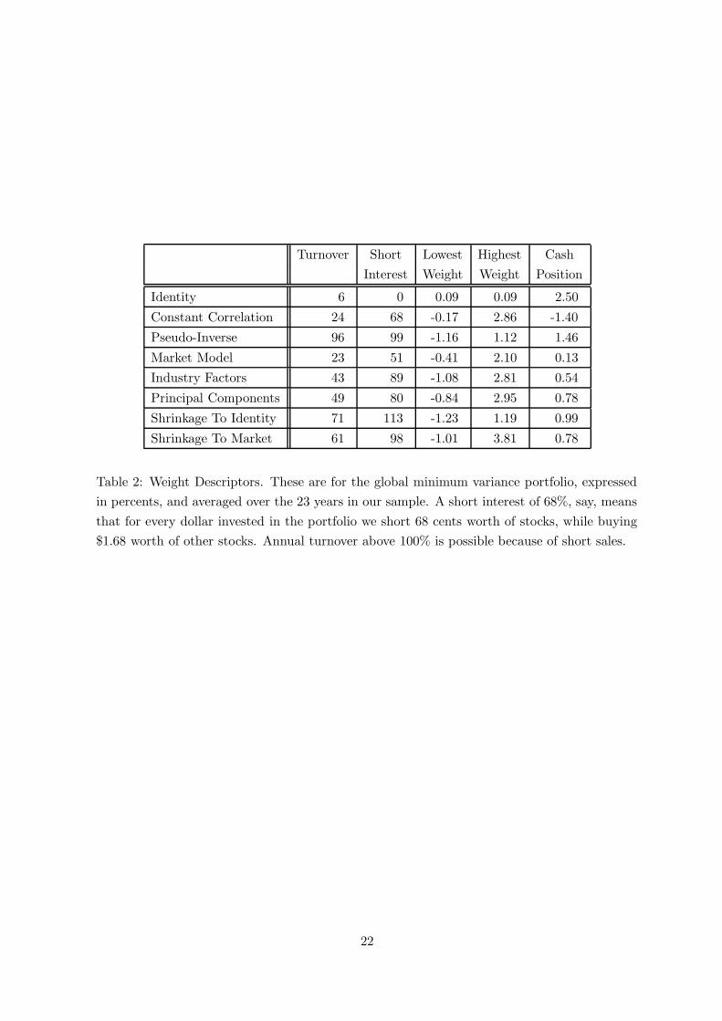
Turnover Short Lowest Highest Cash

Interest Weight Weight Position

Identity 6 0 0.09 0.09 2.50

Constant Correlation 24 68 -0.17 2.86 -1.40

Pseudo-Inverse 96 99 -1.16 1.12 1.46

Market Model 23 51 -0.41 2.10 0.13

Industry Factors 43 89 -1.08 2.81 0.54

Principal Components 49 80 -0.84 2.95 0.78

Shrinkage To Identity 71 113 -1.23 1.19 0.99

Shrinkage To Market 61 98 -1.01 3.81 0.78

Table 2: Weight Descriptors. These are for the global minimum variance portfolio, expressed

in percents, and averaged over the 23 years in our sample. A short interest of 68%, say, means

that for every dollar invested in the portfolio we short 68 cents worth of stocks, while buying

$1.68 worth of other stocks. Annual turnover above 100% is possible because of short sales.

22

1975 1980 1985 19900

0.2

0.4

0.6

0.8

1

Year

Shr

inka

ge I

nten

sity

Figure 2: Optimal Shrinkage Intensity Estimate. This is the weight k/T placed on the single-

index model covariance matrix, as defined by Theorem 2.

23