improved imaging through anisotropic depth migration … · improved imaging through anisotropic...

$: Improved imaging through anisotropic depth migration … · Improved Imaging through Anisotropic Depth Migration and High-Resolution Shallow Tomography In Lieu Of Refraction Statics$
Improved Imaging through Anisotropic Depth Migration and High-Resolution Shallow Tomography In Lieu Of Refraction Statics in South Timbalier Trench Area of Gulf of Mexico: A Case History Gary Rodriguez, Sherry Yang, Diane Yang, Quincy Zhang, Steve Hightower, TGS-NOPEC Geophysical Company Summary We present a case study of an anisotropic prestack depth migration (APSDM) project which used high-resolution, shallow tomography and anisotropic model building for a large depth migration project in the Gulf of Mexico. The enhanced work flow resulted in high quality images and more accurate placement of events, compared to previous processing in the area. The project consisted of approximately 553 OCS blocks of data in the Mississippi Canyon, South Timbalier, Ewing Bank, Grand Isle, Grand Isle South Addition and Ship Shoal South Addition areas (Figure 1). The goals of this project were to produce a more accurate velocity model which would enhance event placement and improve the imaging of steep dips, salt boundaries, and subsalt events. To this end, the low velocity South Timbalier trench area which was previously addressed via refraction statics was modeled using tomographic velocity inversion to produce a more accurate shallow velocity field. Additionally anisotropic prestack depth migration was employed to better tie the seismic events with well information. Introduction This survey is located in an area of the Gulf of Mexico with many complex surface structures and geologic challenges. In the previous processing of this project, long period refraction static corrections and short period surface consistent static corrections were applied in the time domain prior to migration. Traditional refraction statics solutions address the time delays caused by shallow velocity anomalies via static shifts. The slow velocity layer that is solved in the refraction solution will cause “sags” in the resultant seismic image due to the longer travel times through the slow velocity layer. The refraction solution solves for the travel-time delay induced by the layer and applies a static shift to the traces so as to minimize the resultant time sag. While these static shifts generally produce much improved time images deeper in the section, the time static applied is not kinematically correct for depth migration. In particular, this could lead to velocity distortions when solving for the depth velocity field.

While reviewing the velocity modeling approach for this project, it was decided that a high-resolution tomographic inversion would be attempted to more correctly model the velocities in the South Timbalier trench area. If correctly modeled, a more stable velocity field and a more accurate depth image should be expected. It was not presumed that tomography could resolve the high frequency nature of the surface consistent residual statics that had been applied, so this part of the pre-migration data preparation was retained. The other key enhancement to the previous processing flow was the use of anisotropic prestack depth migration. Through the use of abundant checkshot velocity information (539 checkshots) and anisotropic parameter estimation, well-calibrated velocities could be used for migration. The use of a calibrated velocity field should ensure better well ties with seismic data. Initial Anisotropic Model Building A total of 539 checkshots were analyzed for use as a starting point for building the initial velocity model. The checkshot velocity functions were analyzed and spurious trends were edited. These edited checkshot velocities were gridded, interpolated and smoothed to generate the initial vertical velocity model Vz. An isotropic Kirchhoff migration was run using the Vz model. The resultant image gathers were used in a two-parameter semblance scan. The semblance cube that was generated had three axes, which consisted of: depth, epsilon, and delta (two of Thomsen’s weak anisotropic parameters, Thomsen, 2002). The maximum semblance on each of these depth slices would occur at the epsilon and delta values that would best flatten the gather at that depth. A semblance cube was generated for each of the key well locations. The semblance cubes were automatically scanned to estimate the optimal epsilon and delta trends. These epsilon and delta curves were then smoothed, interpolated and gridded to populate the 3D model. To verify the integrity of the epsilon and delta fields, these fields were used to remigrate the data, this time using anisotropic Kirchhoff prestack depth migration. Gather flatness, event focusing, and well ties were checked.

527SEG Houston 2009 International Exposition and Annual Meeting

Downloaded 03 Nov 2009 to 192.160.56.254. Redistribution subject to SEG license or copyright; see Terms of Use at http://segdl.org/

Improved Imaging from High-resolution, shallow tomography

Another iteration of parameter estimation was run, after which the initial anisotropic sediment model was complete.

High Resolution Trench Tomography The resultant Vz, epsilon and delta fields were then used as a starting point for tomographic velocity updating. A full volume high resolution anisotropic prestack depth migration was run over the trench area. Typical model building runs output 10m depth steps with 300m between output offsets (input offset increment of 150m). In order to correctly derive residual curvature estimates for the shallow data, a finer offset and depth sampling were deemed necessary. Consequently, for these iterations a depth step of 5m was used, and the output offset increment was 150m. Furthermore, the tomography inversion cell size was made finer. These early iterations were, however, limited in depth to 4km. The APSDM gathers were scanned for residual curvature. These values along with derived dip fields were input into the first tomographic inversion. In evaluating the residual curvature picks it was noted that there was a strong correlation between areas of positive residual curvature and the previously derived refraction statics solution. Positive curvature is defined as having an increasing reflection depth with increasing offset; thus a positive residual curvature would in general require a slowdown in velocity

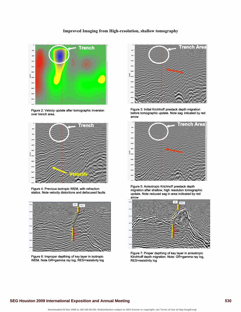
in order to flatten gathers. A shallow slow velocity region is exactly what one would expect in the unconsolidated Timbalier trench area. Shown in Figure 2 is the perturbation of velocity that was output from the tomographic update. The blue-gray region of this display is an area of negative velocity updates (velocity slowdown). Figure 3 shows the seismic data migrated with the initial velocity model. The white circle indicates the trench area. This correlates well with the regions of negative velocity updates that are shown in Figure 2. Figure 5 shows the result of migrating with the updated velocity model. Below the trench area, much better event continuity is seen. The faults imaged much better, and, in general, reflectors seem more geologically straightforward. The red arrow seen in Figure 3 highlights an event “sag” that is induced by the slow velocity anomaly. The red arrow in Figure 5 shows the same area after tomographic velocity updates. The sub-trench events do not have this velocity “sag”. This is contrasted with the image obtained by migrating with the data that had refraction statics applied before migration and velocity updates. This image is shown in Figure 4. The original migration using refraction statics seemed to have false structures induced by distortions in the velocity model. Velocity Model Updating The anisotropic sediment model was further updated with two passes of grid based tomography. These iterations went to a total depth of 12km. This iteration was output with a 10m depth step and 300m offset increment. For each of the tomography iterations, 3D anisotropic prestack Kirchhoff depth migration was run and residual curvature analysis was performed on the resulting image gathers. Automatic dip estimation was performed on the stack volume for use in the tomography ray tracing steps. A new dip field was created for each of the iterations that were run. Any rays traveling through salt were not used in the tomography matrix solution. Vz was updated from the inversion results, and well ties were rechecked and recalibrated. After recalibration of the velocity field, the epsilon and delta fields were then adjusted in order to preserve both flatness of the resultant gathers and the tie to the checkshots. Accounting for the shallow trench area allowed for better imaging and placement of events around this area. Because the imaging was more accurate, sub-trench structures, including salt, were more correctly shaped and positioned. This in turn allowed for a more accurate dip field and, therefore, better tomographic velocity updates below the trench. Having this shallow slow velocity region in the

Figure 1: Map showing the location of the survey area




model had a positive influence in the region allowing for more accurate velocities and images all around. The salt geometry was quite complex. In order to correctly define salt overhangs, the salt geometry was defined using 4 passes of APSDM. Initially, top of salt was picked on the image produced by migration with the final supra-salt sediment velocity field. At this stage salt boundaries interpreted from the seismic images were checked against top salt events picked from well data. Vz, epsilon, and delta were then adjusted accordingly in order for salt tops to image at the proper depths, while simultaneously preserving the image gather flatness. The first base of salt was interpreted on seismic images produced after APDSM using the recalibrated salt flooded velocity model. A migration was then run with the first top and base of salt inserted into the model, and second (deeper or overhang) top salts were interpreted. Next APSDM was run which flooded below the second top salt. The second base salt was interpreted and the final salt model was constructed using these four surfaces. The data was then migrated with the interpreted salt geometry. A final tomography pass was performed for the sub-salt areas. In this iteration, sedimentary regions of the model, both under salt and away from the salt were updated. Tomography inverted for the velocity updates which were subsequently added back to the previous sediment model. Salt was inserted back into the final sediment model to produce the final salt model. The final imaging step was run with the anisotropic prestack Kirchhoff depth migration using an increased aperture. To better image steep dip salt flanks turning rays were also used in the migration. Figure 6 shows a section from the previous processing effort. The red line on the section is the resistivity log from the well whose track is shown by the black line in the section. The yellow line is the gamma ray log from the same well. The characteristic kicks at the top and base salt show that that salt is mis-positioned in this image. Salt is imaged deeper than the well would indicate. Contrasted with the isotropic migration in Figure 6 is the anisotropic depth image shown in Figure 7. Note that the APSDM result has a much better tie to the gamma ray and resistivity logs at both salt-sediment interfaces. Additionally the steeply dipping salt structures are imaged significantly better than the previous results. Furthermore, the improved definition of the top salt geometry has resulted in a better focused base salt image as well as better subsalt images.

Conclusions The enhanced workflow for this project included the using a well-tied anisotropic sediment model, anisotropic prestack Kirchhoff depth migration, modeling of salt bodies with overhangs, and iterations of both supra-salt and subsalt tomography, including two shallow, high-resolution iterations. This methodology resulted in a high-quality image with more accurate event placement and geologic structures. Salt boundaries and steep or overturned events were imaged much better that in previous processing. Deep structures and subsalt events were more geologically sensible and had increased continuity. Addressing the slow velocity zone via tomography rather than using a refraction statics solutions resulted in better focused shallow faults and more realistic structures in the Timbalier trench area. Acknowledgments The authors would like to thank their colleagues who help in reviewing this paper and suggesting changes. These include, Laurie Geiger, Michael Ball, Connie Gough, Bin Wang and Zhiming Li. Thanks also to TGS for allowing this work to be published.




Trench

Trench

Velocity

Figure 6: Improper depthing of key layer in isotropic WEM. Note GR=gamma ray log, RES=resistivity log

Figure 4: Previous isotropic WEM, with refraction statics. Note velocity distortions and defocused faults

Figure 2: Velociy update after tomographic inversion over trench area.

Trench Trench Trench

Trench

Velocity

Trench Trench

Velocity

Figure 6: Improper depthing of key layer in isotropic WEM. Note GR=gamma ray log, RES=resistivity log

Figure 4: Previous isotropic WEM, with refraction statics. Note velocity distortions and defocused faults

Figure 2: Velociy update after tomographic inversion over trench area.

Trench Area

Trench Area

Figure 3: Initial Kirchhoff prestack depth migration before tomographic update. Note sag inticated by red arrow

Figure 5: Anisotropic Krichhoff prestack depth migration after shallow, high resoluton tomographic update. Note reduced sag in area indicated by red arrow

Figure 7: Proper depthing of key layer in anisotropic Kirchhoff depth migration. Note: GR=gamma ray log, RES=resistivity log

Trench AreaTrench AreaTrench Area

Trench AreaTrench AreaTrench Area

Figure 3: Initial Kirchhoff prestack depth migration before tomographic update. Note sag inticated by red arrow

Figure 5: Anisotropic Krichhoff prestack depth migration after shallow, high resoluton tomographic update. Note reduced sag in area indicated by red arrow

Figure 7: Proper depthing of key layer in anisotropic Kirchhoff depth migration. Note: GR=gamma ray log, RES=resistivity log



EDITED REFERENCES Note: This reference list is a copy-edited version of the reference list submitted by the author. Reference lists for the 2009 SEG Technical Program Expanded Abstracts have been copy edited so that references provided with the online metadata for each paper will achieve a high degree of linking to cited sources that appear on the Web. REFERENCES None



improved imaging through anisotropic depth migration … · improved imaging through anisotropic...

Documents