improvedvirtualpotentialfieldalgorithmbasedonprobability...

Hindawi Publishing CorporationInternational Journal of Distributed Sensor NetworksVolume 2012, Article ID 942080, 9 pagesdoi:10.1155/2012/942080

Research Article

Improved Virtual Potential Field Algorithm Based on ProbabilityModel in Three-Dimensional Directional Sensor Networks

Junjie Huang,1 Lijuan Sun,2 Ruchuan Wang,2 and Haiping Huang2

1 College of Internet of Things, Nanjing University of Posts and Telecommunications, Jiangsu High Technology Research Key Laboratoryfor Wireless Sensor Networks, and Key Lab of Broadband Wireless Communication and Sensor Network Technology, Ministry ofEducation, Nanjing 210003, China

2 College of Computer, Nanjing University of Posts and Telecommunications, Jiangsu High Technology Research Key Laboratoryfor Wireless Sensor Networks, and Key Lab of Broadband Wireless Communication and Sensor Network Technology, Ministry ofEducation, Nanjing 210003, China

Correspondence should be addressed to Junjie Huang, [email protected]

Received 2 November 2011; Revised 12 March 2012; Accepted 13 March 2012

Academic Editor: Sabah Mohammed

Copyright © 2012 Junjie Huang et al. This is an open access article distributed under the Creative Commons Attribution License,which permits unrestricted use, distribution, and reproduction in any medium, provided the original work is properly cited.

In conventional directional sensor networks, coverage control for each sensor is based on a 2D directional sensing model. However,2D directional sensing model failed to accurately characterize the actual application scene of image/video sensor networks. Toremedy this deficiency, we propose a 3D directional sensor coverage-control model with tunable orientations. Besides, a novelcriterion for judgment is proposed in view of the irrationality that traditional virtual potential field algorithms brought about onthe criterion for the generation of virtual force. Furthermore, cross-set test is used to determine whether the sensory region has anyoverlap and coverage impact factor is introduced to reduce profitless rotation from coverage optimization, thereby the energy costof nodes was restrained and the performance of the algorithm was improved. The extensive simulations results demonstrate theeffectiveness of our proposed 3D sensing model and IPA3D (improved virtual potential field based algorithm in three-dimensionaldirectional sensor networks).

1. Introduction

The sensory ability of WSNs to physical world is embodiedin coverage which is often used to describe the monitoringstandard of Quality of Service (QoS) [1, 2]. Coverage opti-mization in sensor networks plays a significant role inallocating network space, realizing context awareness andinformation acquisition, and enhancing the viability ofnetworks [3].

Early studies on coverage optimization were based ontwo-dimensional sensory domain model [4, 5], or 0-1 proba-bility sensory model. For instance, the virtual force algorithm(VFA) proposed by Zou and Chakrabarty [6] moves nodesafter all nodes’ moving paths have been determined. Theauthors of [7] proposed an approximate centralized greedalgorithm to solve the maximum coverage problem withminimum sensors. Coverage in terms of the number oftargets to be covered is maximized, whereas the number of

sensors to be activated is minimized. The target involvedvirtual force algorithm (TIVFA) is proposed by Li et al.[8] and potential field-based coverage-enhancing algorithm(PFCEA) aiming at directional sensor model is proposedby Tao et al. [9]. The authors of [10] discussed multipledirectional cover sets problem of organizing the directionsof sensors into a group of nondisjoint cover sets in each ofwhich the directions cover all the targets so as to maximizethe network lifetime. In [11], which is written by me, Iimproved the criterion for judging the generation of virtualpotential field via cross-set test. However, probability-basedthree-dimensional sensor networks model is more tendingto be in conformity with practical application, for example,the recently arisen multimedia sensor networks [3, 12–16]and underwater networks [17]. In view of three-dimensionalsensory model and probability sensory model, overseas anddomestic researchers have yielded some research achieve-ments on coverage algorithms in recent years. I proposed

2 International Journal of Distributed Sensor Networks

a virtual force algorithm which is applicable with three-dimensional omnidirectional sensory model in [18]. Authorsof [19] put forward a three-dimensional directional sen-sory model and optimized coverage performance usingvirtual potential field and simulated annealing algorithm.Reference [20] proposed a coverage configuration algorithmbased on probability detection model (CCAP). Reference[21] proposed a coverage preservation protocol based onprobability detection model (CPP) that makes workingnodes in sensor networks as few as possible when networkcoverage is guaranteed. However, this protocol configuresnetwork using centred control algorithm which limits thenetwork scale, and at present most of the literatures havenot introduced this probability coverage model into three-dimensional sensor networks. In fact, most practical appliedwireless sensor networks are deposited in three-dimensionalsensor networks so that it will be more accurate if it issimulated in a three-dimensional space [22, 23]. In [22], Baiet al. proposed and designed a series of connected coveragemodel in three-dimensional wireless sensor networks withlow connectivity and full coverage. In [23], Alam andHaas studied truncated octahedron deployment strategy tomonitor network coverage situation. But in most studies,the criterion for the generation of repulsion between twopoints is simply defined as the situation that the distancebetween nodes is less than twice the sensory radius, whichhas been proved inappropriate to directional sensor networksin [11] by me. Therefore, first we analyze the sensoryability of three-dimensional directional sensor based onprobability model to design a novel direction-steerablethree-dimensional directional sensor model and make useof virtual potential algorithm to adjust node directionto improve coverage effect. In particular, in this paperwe proposed a more rational criterion for generation ofrepulsion in three-dimensional directional sensor networksand introduced a factor called coverage impact factor toestimate the impact on network coverage from the change ofsensing direction in advance, to reduce profitless adjustmentof sensing direction, save node energy, enhance algorithmperformance, and optimize coverage effect.

This paper is organized as follows: Section 2 gives theproblem description and related definition. Section 3describes the improved virtual potential field-based algo-rithm in three-dimensional directional sensor networksbased on probability model. Section 4 describes in detail thealgorithm flow. Section 5 verifies the validity of the algorithmvia simulation experiments and makes contrast. Section 6draws conclusion.

2. Coverage Enhancement Issues ofThree Directional Sensor Networks

2.1. Problem Formulation. The coverage enhancement issueof three directional sensor networks that is constituted bydirection-steerable nodes can be described as follow: howto enhance the degree of coverage by changing the sensingdirection so that degree of coverage in target area approachesmaximum in condition that a certain number of nodes are

randomly distributed in a given three-dimensional targetarea and part of the area is not covered by nodes and thenumber and position of nodes are stable.

2.2. Analysis and Definitions on Coverage Enhancement Issuein Directional Sensor Networks. For the purpose of laterresearch, we give the consumptions beforehand, shown asfollows.

(1) Every node works independently, namely, sensorytask of each node does not depend on others’.

(2) All nodes are isomorphic, namely, all the maximumsensory distance RS, sensory deviation angle α, andcommunication radius RC are equal, respectively, andthe communication radius is no less than twice of themaximum sensory distance.

(3) Every node can get the information of its location andsensing direction and the direction is steerable.

Limited by the angle of view, the sensory area of the

directional sensor model is abstracted to a tetrad 〈L,RS, �D,α〉in three-dimensional space. As shown in Figure 1.

Definition 1 (directional sensor model 〈L,RS, �D,α〉). L islocation of nodes, that corresponds to (x, y, z) in a three-dimensional rectangular coordinate system. RS is maximum

sensory distance of nodes. �D is unit vector of sensingdirection, denoted by (dx,dy,dz), whose direction andcentral axis of sensory region is collinear. α is called sensorydeviation angle and 0 ≤ α ≤ π.

In particular, when α = π, the sensory region is a spherethus the traditional omnidirectional sensor model can beconsidered as a special case of directional sensor model.

Definition 2 (probability detection model). In this part, wedefine the sensor sensing accuracy model. Sensing accuracyof sensor Si at point t is defined as the probability of sensor Sito successfully detect an event happening at point t. A pointhere means a physical location in the covered area.

We assume that a sensor can always detect an eventhappening at the point with distance 0 from the sensor,and the sensing accuracy attenuates with the increase of thedistance. One possible sensing accuracy model is [24]

Pit = 1

(1 + ∂dit)β , (1)

where Pit is the sensing accuracy of sensor Si at point t, ditis the distance between sensor Si and point t, and constants∂ and β are device-dependent parameters reflecting thephysical features of a sensor. Generally, β ranges from 1 to4. And ∂ is used as an adjustment parameter.

Sensor node density is usually higher. Assume thatN sen-sor nodes are randomly distributed in a three-dimensionalmonitoring area. Therefore, events in the monitoring area are

International Journal of Distributed Sensor Networks 3

D(dx , dy , dz)α

α

L(x, y, z) Rs

Figure 1: Directional sensor model.

detected by multiple sensor nodes simultaneously. The senseprobability is expressed as follow:

Pt = 1−N∏

i=1

(1− Pit). (2)

Substitute into Formula (1)

Pt = 1−N∏

i=1

(1− 1

(1 + ∂dit)β

). (3)

According to (3), Pt ≥ Pit, because multiple sensor nodesmay sense the same events simultaneously.

Definition 3 (maximum sensory distanceRS). The maximumsensory distance of nodes is defined as

RS = 1∂

(λ−1/β − 1

). (4)

In condition of node si working independently, if dit ≥RS, the probability of node si being detected is Pit = 1/(1 +∂dit)

β ≤ λ. In this case, the effect on system detectionprobability from node si to target point can be ignored.λ is the minimum probability of target found, which isdetermined by the actual application environment, hardwareand software conditions and quality of service required, andother factors. λ is usually specified by user.

Definition 4 (sensory domain of node si). For ease of latercalculation, we translate the directional sensor model in Fig-ure 1 into that in Figure 2 and give the following definition.

The sensory region is part of a sphere that centred on�D with radius RS and maximum rotation angle which isdenoted by SDi. In other words, sensory region is constitutedby all spots that satisfy Formula (1) in which x representsspots in space, θi represents the intersection angle with

sensing direction vector �D

SDi = {x | ‖x − si‖ ≤ RS, |θi(x)| ≤ α}. (5)

x

θi(x)

D(dx , dy , dz)

α

α

L(x, y, z) Rs

Figure 2: Sensory domain of node.

Definition 5 (Set of neighbor nodes ψi). In sensor network,two nodes are called neighbors when Euclidean distance isless than twice the maximum sensory distance RS. The set ofneighbor nodes of node si is ψi

ψi ={s j | D

(si, s j

)< 2Rs, i /= j

}. (6)

Definition 6 (γ-probability coverage). In a set of activenodes located at (xi, yi, zi), i = 1, 2, . . . ,N , system detectionprobability of target point located at (xt, yt, zt) is Pt . If Pt �γ, the target point located at (xt, yt, zt) is satisfied with γprobability coverage. If all points in a region are satisfied withγ probability coverage, then this region is called complete γprobability coverage.

Definition 7 (degree of coverage). A given area S is equallydivided into M small areas which can be assumed as pointsas M is large enough. If there are Q points in the M pointsthat accord with γ-probability coverage, coverage rate of areaS is defined as

DoC(S) = Q

M. (7)

Definition 8 (coverage impact factor). Coverage impactfactor μ characterizes the impact on network coverage whenthe sensing direction angle has been changed. We define it asfollows:

μ =⎧⎨⎩

1, DoC′i (S) > DoCi(S),

0, DoC′i (S) ≤ DoCi(S).(8)

DoC′i (S) represents the network coverage after node si hasbeen changed.

3. The Improved Virtual Potential Field-BasedAlgorithm in Three-Dimensional DirectionalSensor Networks

Taking the deployment cost of sensor network into consider-ation, it would be unpractical that all nodes are capable of


moving. Moreover, the movement of sensor nodes usuallycauses the invalidation of part of sensor nodes and in turnchanges the topology of the whole sensor network. All thesefactors raise the maintenance cost of network. Therefore, weassume that all nodes remain at the same location as initialand coverage can be enhanced by changing sensing directionof nodes. We introduce the concept of centroid. ci representsthe centroid that is relative to node si and locates in a spot incentral axis of sensory region with a distance of 2Rsinα/3αapart from the node. Now the issue is translated into thevirtual force issue between centroids. We assume that thereis virtual repulsion Frep between centroids. Under the actionof repulsion, two nodes rotate in opposite direction to avoidthe formation of sensory overlap region. At the same timeof reducing the redundant coverage, a sufficient and efficientcoverage of the monitoring area is achieved. Under the actionof virtual potential field, every node gets the repulsion fromone or more adjacent nodes.

3.1. Judgement on Overlap Situation of Sensory Area. Intraditional algorithms, which use the virtual potential field toenhance coverage, the criterion for the generation of repul-sion between two points is that the distance between nodesis less than 2RS [7] which is applicable to omnidirectionalsensor model in that when the distance between nodes isless than 2RS, there bound to be some overlap in sensoryarea. But with regard to directional sensor model, the aboveconclusion is obviously incorrect. As shown in Figure 3, twonodes are less than 2RS apart from each other; however, withno sensory overlapped region for the difference of sensingdirection angle. As a case by case, Figure 3 reflects a commonsituation in many cases which causes profitless adjustment ofdeployment, wastes energy of nodes, and shortens networklifetime.

Therefore, in this paper, the criterion for generation ofrepulsion between two nodes is defined as whether or notthere is overlap sensory region between two nodes.

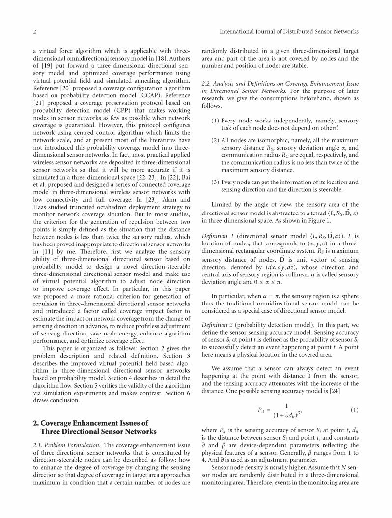
To three-dimensional directional sensor networks model,when judging whether there is overlapped sensory regionbetween two nodes, we project the sensory region ontoplanes xoy, xoz, and yoz in a three-dimensional rectangularcoordinate system. If and only if all projections on threeplanes has overlapped region, does the sensory region hasoverlapped region. So the overlap decision problem of three-dimensional sensor model has translated into that of two-dimensional model. I put forward an approach in [11] todecide if there is overlapped region in a two-dimensionaldirectional sensor network model using cross-set test. Refer-ence [25] demonstrates the 11 kinds of overlapped situationsof sensory region with two-dimensional directional sensormodel, as shown in Figure 4.

We simplify the sectorial sensor model of a two-dimensional space into a triangle by replacing the arc insector by line, because only under the circumstances of (c)and (d) in Figure 4 can the decision outcome be different.It can be seen in Figure 4 that the area of the overlap regionunder the two circumstances is small compared to the wholesensory region, so it is inefficient to waste energy and adjustdeployment of nodes for that purpose.

Sj

Si

Figure 3: A case that distance is less than 2RS without overlappedsensory region.

After simplifying, we can determine whether the twotriangles have overlap region according to whether theyhave intersecting sides by mean of cross-set test. As shownin Figure 5, a triangle with overlap region must haveintersecting sides. For example, in Figure 5, S1a1 and S2a2

intersect, the following must be satisfied:

[(a2 − S1)× (a1 − S1)]∗ [(a1 − S1)× (S2 − S1)] ≥ 0,

[(S1 − a2)× (S2 − a2)]∗ [(S2 − a2)× (a1 − a2)] ≥ 0.(9)

3.2. Analysis on Regulation of Node Rotation

3.2.1. Analysis on Regulation of Centroids. Nodes si and s j areneighbors, the centroid ci at location Xi is under action of therepulsion of cj at location X j which is defined as follows:

Frep(i, j) =

⎧⎪⎪⎪⎨⎪⎪⎪⎩

krep

D(ci, cj

)2

⎛⎝ xi − x j

D(ci, cj

)

⎞⎠, SDi ∩ SDj /=∅,

0, SDi ∩ SDj = ∅.(10)

Using the method of Section 3.1, only when there isoverlap region between two nodes, repulsion between cen-troids of two nodes exists. D(ci, cj) represents the Euclideandistance between centroid ci and cj . krep represents therepulsion coefficient which is a positive constant. SDi/SDj

represent sensory domain of node si/s j . The magnitudeof repulsion of centroid is inversely proportional to theEuclidean distance between them and the direction ofrepulsion that the centroid ci taking action is determinedby the location of ci and cj . The resultant force Frep(i) ofrepulsion at centroid ci is

Frep(i) =∑

nj∈ψiFrep

(i, j), (11)

ψi represents the set of all the neighbors of node si.

3.2.2. Analysis on Rotation Angle. The resultant repulse forceactions on centroid ci and node single rotation angle θ jointlydecide the later target location X′i of centroid ci. Thereby, the


(a) (b) (c) (d)

(e) (f) (g) (h)

(i) (j) (k)

Figure 4: The situations of overlap of sensory region in directionalsensor model.

a2

a1

b1

b2

S2

S1

Figure 5: Two sensor models with overlap sensory region.

later target location of centroid ci can be described as rotatinga certain angle θ along the direction of resultant force Frep.Use Formula (5) to calculate the coverage impact factor. Ifμ = 1, which means the movement is beneficial to coverageoptimization, proceed the node rotation. Otherwise, thecurrent sensing direction remain unchanged. Repeatedly,optimal solution approaches by fine adjustment. Meanwhile,we set the force threshold ε. When ‖FT‖ ≤ ε, centroid willoscillate repeatedly around a certain point which can beregarded as a stable state of centroid and no more actionsis required. When all centroids come to the stable statewithin the network, the whole sensor network is consideredas having reached the stable state.

4. Algorithm Description

According to the virtual force of the centroid of eachnode, a node deployment adjustment algorithm is proposedas follows in this paper. The algorithm is a distributedalgorithm and executes simultaneously in each node. We

equally divided the sensing area S into M small areas. M islarge enough so that the small areas could be assumed aspoints. When area degree of coverage is calculated accordingto formula (7), the target point should be satisfied with γ-probability coverage. Take node si for example, Formalizeddescription of the algorithm is as in Algorithm 1.

5. Algorithm Simulations andPerformance Analysis

We developed the simulation software Sencov3.0 that appli-cable to the research of sensor network deployment andcoverage with VC++6.0, using which we verify the validity ofIPA3D algorithm through extensive simulation experiments.Values of specific parameters are shown in Table 1. We cansee from formula (4) that RS is determined by ∂, β, λ. In allsimulation experiments of this paper, we set ∂ = 1 and β = 1,so the value of RS is only determined by λ.

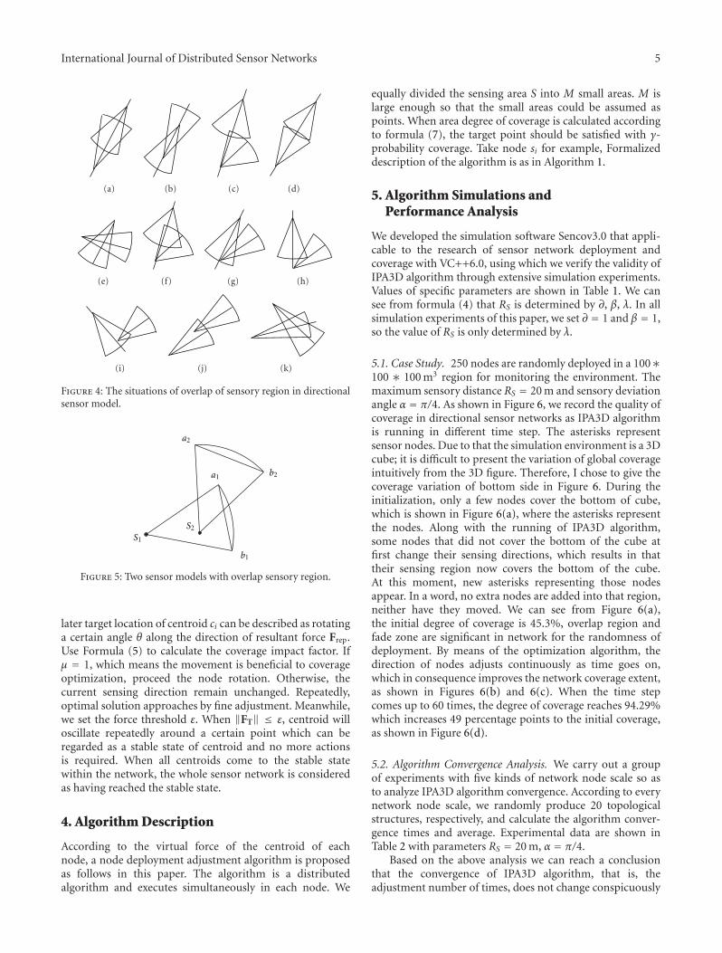
5.1. Case Study. 250 nodes are randomly deployed in a 100∗100 ∗ 100 m3 region for monitoring the environment. Themaximum sensory distance RS = 20 m and sensory deviationangle α = π/4. As shown in Figure 6, we record the quality ofcoverage in directional sensor networks as IPA3D algorithmis running in different time step. The asterisks representsensor nodes. Due to that the simulation environment is a 3Dcube; it is difficult to present the variation of global coverageintuitively from the 3D figure. Therefore, I chose to give thecoverage variation of bottom side in Figure 6. During theinitialization, only a few nodes cover the bottom of cube,which is shown in Figure 6(a), where the asterisks representthe nodes. Along with the running of IPA3D algorithm,some nodes that did not cover the bottom of the cube atfirst change their sensing directions, which results in thattheir sensing region now covers the bottom of the cube.At this moment, new asterisks representing those nodesappear. In a word, no extra nodes are added into that region,neither have they moved. We can see from Figure 6(a),the initial degree of coverage is 45.3%, overlap region andfade zone are significant in network for the randomness ofdeployment. By means of the optimization algorithm, thedirection of nodes adjusts continuously as time goes on,which in consequence improves the network coverage extent,as shown in Figures 6(b) and 6(c). When the time stepcomes up to 60 times, the degree of coverage reaches 94.29%which increases 49 percentage points to the initial coverage,as shown in Figure 6(d).

5.2. Algorithm Convergence Analysis. We carry out a groupof experiments with five kinds of network node scale so asto analyze IPA3D algorithm convergence. According to everynetwork node scale, we randomly produce 20 topologicalstructures, respectively, and calculate the algorithm conver-gence times and average. Experimental data are shown inTable 2 with parameters RS = 20 m, α = π/4.

Based on the above analysis we can reach a conclusionthat the convergence of IPA3D algorithm, that is, theadjustment number of times, does not change conspicuously


//initialization(1) t ←0;(2) set the maximum cycle index tmax;(3) determine the initial position of corresponding centroid ci

of si and neighbor nodes set ψi.(4) while (t < tmax) do(5) renew the current coordinate position of centroid ci;(6) determine the repulsion force Frep(i) acting on centroid ci from other nodes according to formula (10) and (11)(7) if (‖Frep(i)‖ ≥ ε) then(8) determine the later target location X′i of centroid ci decided by the resultant repulse force actions on

centroid ci and node single rotation angle θ(9) calculate the coverage impact factor μ of angle rotation this time according to Formula (8)(10) if μ = 1, proceed the angle rotation, else remain the sensing direction unchanged(11) else break;(12) t ← t + 1(13) end.

Algorithm 1

Table 1: Experiment parameters.

Parameter name Parameter values

Target region 100∗ 100∗ 100 m3

Distribution mode Uniform distribution

Number of nodes N 100–300

Device-dependent parameter ∂, β 1, 1

Minimum probability of targetfound λ

0.32–0.91

γ-probability coverage 0.90

Sensory angle of deviation α π/6, π/5, π/4, π/3, π/2, π

Repulsion coefficient krep 100

Table 2: Convergence analysis on experimental data.

Number ofnodes N

Initial degreeof coverage %

Ultimate degreeof coverage %

Cycleindex t

100 18.30 42.15 74.5

150 27.42 61.53 77.7

200 38.65 81.77 75.6

250 46.32 93.59 78.9

300 52.51 95.14 72.3

along with sensor network node scale. The value ranges from70 to 80; thus IPA3D algorithm has a nice convergence.

5.3. Comparative Analysis of Algorithms. In this section, aseries of simulation experiments are conducted to illustratethe effect on the performance of IPA3D algorithm from thethree key parameters. They are node scale N , maximumsensory distance RS, and sensory deviation angle α. Reference[9] takes traditional basis as the criterion for the generationof repulsion. We compare it to the coverage enhancement

algorithm proposed in this paper and analyze their perfor-mances.

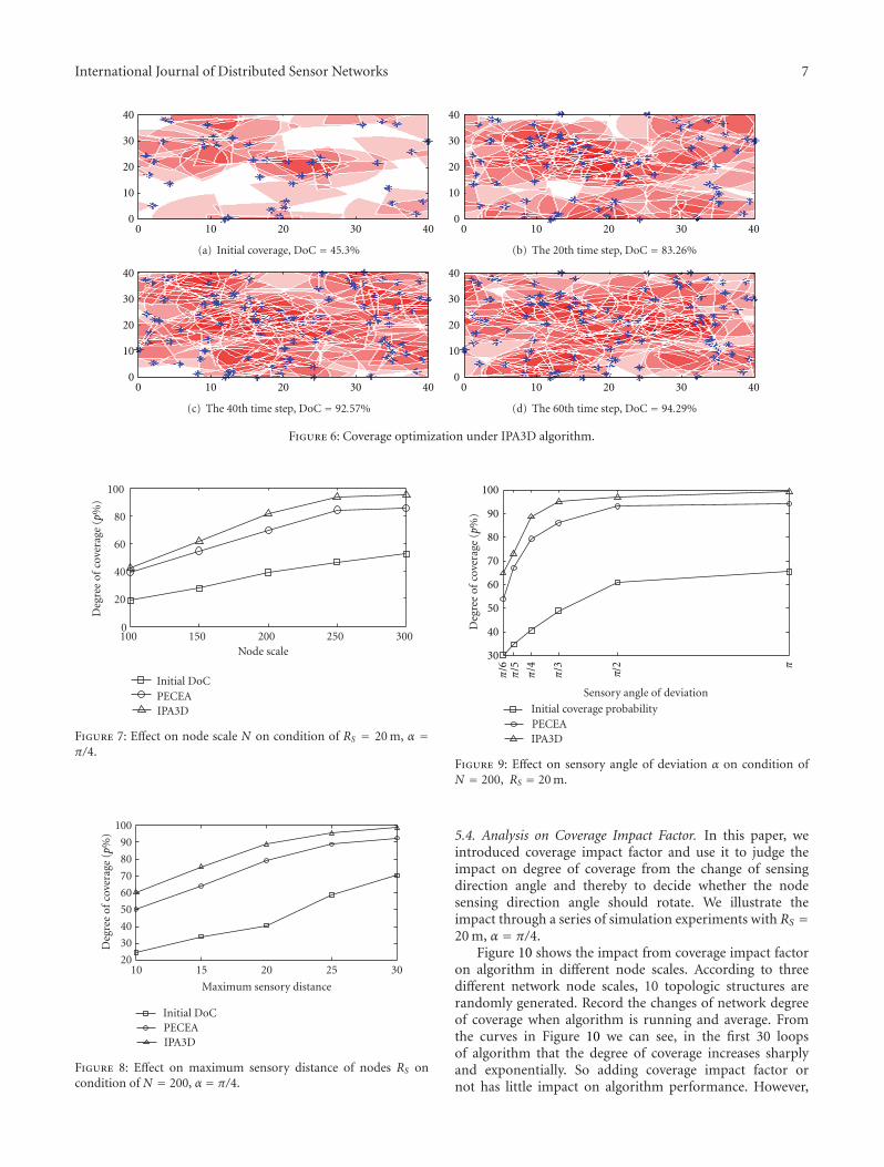
It can be seen from the curve in Figure 7 that when RSand α are fixed, smaller value leads to less initial degree ofcoverage. With the increasing of node scale N , the valueof Δp shows an upward trend. Δp means the differencebetween the final degree of coverage and the initial state.When N = 250, the degree of coverage increases 49percentage points and afterwards value of Δp decreases tosome extent. The reason is that when nodes number reachesa certain scale, optimized network degree of coverage hasapproached extreme and increase of node number can nolonger enhance network coverage conspicuously. Meanwhile,the increase of nodes leads to a higher initial degree ofcoverage and greatly decreases the probability that severalcommunicational adjacent nodes form coverage fade zonewhich undoubtedly weakens the performance of IPA3Dalgorithm.

We can see from the curve in Figures 8 and 9 that theeffect on this algorithm from maximum sensory distanceof nodes RS and sensory deviation angle α is in accordancewith the node scale. When the node scale is fixed, thesmaller maximum sensory distance of nodes RS and sensorydeviation angle α are, the less possible that adjacent nodesare form an overlap region, and the less improvement isdone to the network coverage performance. As the increase ofmaximum sensory distance of nodes, Δp increases constantlytoo. The network degree of coverage reaches the climax whenRS and α are at a particular value. However, with the increaseof the value of RS and α, the probability of creating coveragefade zone becomes smaller which leads to less significanteffect on network degree of coverage enhancement.

As can be seen from Figures 7, 8, and 9 that comparedto the PECEA algorithm in [9], under the same parametervalue, the proposed IPA3D algorithm increases the coveragequality most significantly after the optimization of the initialdeployment, which illustrates the superiority of this algo-rithm.


40

30

20

10

0403020100

(a) Initial coverage, DoC = 45.3%

40

30

20

10

0403020100

(b) The 20th time step, DoC = 83.26%

40

30

20

10

0403020100

(c) The 40th time step, DoC = 92.57%

40

30

20

10

0403020100

(d) The 60th time step, DoC = 94.29%

Figure 6: Coverage optimization under IPA3D algorithm.

100 150 200 250 3000

20

40

60

80

100

Deg

ree

of c

over

age

(p%

)

Initial DoC

Node scale

PECEAIPA3D

Figure 7: Effect on node scale N on condition of RS = 20 m, α =π/4.

10 15 20 25 3020

30

40

50

60

70

80

90

100

Maximum sensory distance

Deg

ree

of c

over

age

(p%

)

Initial DoCPECEAIPA3D

Figure 8: Effect on maximum sensory distance of nodes RS oncondition of N = 200, α = π/4.

Sensory angle of deviation

Initial coverage probabilityPECEAIPA3D

100

90

80

70

60

50

40

30

Deg

ree

of c

over

age

(p%

)

π

π/2

π/3

π/4

π/5

π/6

Figure 9: Effect on sensory angle of deviation α on condition ofN = 200, RS = 20 m.

5.4. Analysis on Coverage Impact Factor. In this paper, weintroduced coverage impact factor and use it to judge theimpact on degree of coverage from the change of sensingdirection angle and thereby to decide whether the nodesensing direction angle should rotate. We illustrate theimpact through a series of simulation experiments with RS =20 m, α = π/4.

Figure 10 shows the impact from coverage impact factoron algorithm in different node scales. According to threedifferent network node scales, 10 topologic structures arerandomly generated. Record the changes of network degreeof coverage when algorithm is running and average. Fromthe curves in Figure 10 we can see, in the first 30 loopsof algorithm that the degree of coverage increases sharplyand exponentially. So adding coverage impact factor ornot has little impact on algorithm performance. However,


0 10 20 30 40 50 60 70 80

30

40

50

60

70

80

90

100

Time (T)

IPA3D (N = 250)IPA3D without factor (N = 250)

IPA3D(N = 200)IPA3D without factor (N = 200)IPA3D (N = 150)IPA3D without factor (N = 150)

Deg

ree

of c

over

age

(p%

)

Figure 10: Impact on algorithm performance from coverage impactfactor in different node scale.

with the increase of algorithm execution time, algorithmdegree of coverage without coverage impact factor presentsa fluctuating state and overall degree of coverage stopsincreasing while algorithm degree of coverage with coverageimpact factor shows a gentle rising trend and finally reachesstable state with degree of coverage remaining unchanged.The reason is that, without coverage impact factor, theforce on a single node is according to neighbor nodesset ψi and the change of sensing direction angle of asingle node cannot take the impact on overall networkcoverage into account and may reduce network degree ofcoverage. And algorithm with coverage impact factor willevaluate the impact on overall coverage every time beforesensing direction is changed to get rid of profitless rotation.Though it may increase algorithm complexity and cost nodeenergy, it is greatly less than the energy cost of profitlessrotation which means movements that cannot give beneficialeffect to network coverage. As shown in Figure 10, to addcoverage impact factor efficiently improved the performanceof coverage enhancement algorithm and overcame the faultof the unstable state in later stage.

6. Conclusions

This paper proposed a probability-based three-dimensionaldirectional sensory model, and based on which a novelcriterion for judgment is proposed in view of the irra-tionality that traditional virtual potential field algorithmsbrought about on the criterion for the generation of virtualforce. Cross-set test was used to determine whether thesensory region has any overlap and coverage impact factoris introduced to reduce profitless rotation from coverageoptimization, thereby the energy cost of nodes was restrained

and the performance of the algorithm was improved. Insimulation experiment, first we verified the convergence ofthe algorithm and then the effect on the algorithm from thekey parameters and the validity of IPA3D were demonstratedby the comparison between IPA3D and PECEA under theeffect of key parameters. Also, we confirmed and analyzedthe impact on IPA3D algorithm from coverage impact factorthrough simulation experiment. The proposed algorithmeffectively improved the coverage performance of traditionalvirtual potential field algorithms but the energy consump-tion caused by the change of sensing direction angle were nottaken into account which is for further study.

Acknowledgments

The subject is sponsored by the National Natural Sci-ence Foundation of China (Nos. 60973139, 61003039,61170065, and 61171053), Scientific and TechnologicalSupport Project (Industry) of Jiangsu Province (Nos.BE2010197, BE2010198), Natural Science Key Fund for Col-leges and Universities in Jiangsu Province (11KJA520001),the Natural Science Foundation for Higher Education Insti-tutions of Jiangsu Province (10KJB520013, 10KJB520014),Academical Scientific Research Industrialization PromotingProject (JH2010-14), Fund of Jiangsu Provincial Key Lab-oratory for Computer Information Processing Technology(KJS1022), Postdoctoral Foundation (1101011B), Scienceand Technology Innovation Fund for Higher EducationInstitutions of Jiangsu Province (CXZZ11-0409), the SixKinds of Top Talent of Jiangsu Province (2008118), DoctoralFund of Ministry of Education of China (20103223120007,20113223110002), and the Project Funded by the PriorityAcademic Program Development of Jiangsu Higher Educa-tion Institutions (yx002001).

References

[1] S. Meguerdichian, F. Koushanfar, M. Potkonjak, and M. B.Srivastava, “Coverage problems in wireless ad-hoc sensornetworks,” in Proceedings of the 20th Annual Joint Conference ofthe IEEE Computer and Communications Societies (INFOCOM’01), pp. 1380–1387, IEEE Press, New York, NY, USA, April2001.

[2] D. Tao, Y. Sun, and H. J. Chen, “Worst-case coverage detectionand repair algorithm for video sensor networks,” Acta Elec-tronica Sinica, vol. 37, no. 10, pp. 2284–2290, 2009.

[3] I. F. Akyildiz, T. Melodia, and K. R. Chowdhury, “A surveyon wireless multimedia sensor networks,” Computer Networks,vol. 51, no. 4, pp. 921–960, 2007.

[4] A. Howard, M. J. Mataric, and G. S. Sukhatme, “Mobile sensornetwork deployment using potential field: a distributed scal-able solution to the area coverage problem,” in Proceedings ofthe 6th International Symposium on Distributed AutonomousRobotics Systems (DARS ’02), pp. 299–308, Fukuoka, Japan,June 2002.

[5] S. Poduri and G. S. Sukhatme, “Constrained coverage formobile sensor networks,” in Proceedings of the IEEE Interna-tional Conference on Robotics and Automation, pp. 165–171,IEEE Press, New York, NY, USA, May 2004.


[6] Y. Zou and K. Chakrabarty, “Sensor deployment and targetlocalization in distributed sensor networks,” ACM Transac-tions on Embedded Computing Systems, vol. 3, no. 1, pp. 61–91,2004.

[7] J. Ai and A. A. Abouzeid, “Coverage by directional sensors inrandomly deployed wireless sensor networks,” Journal ofCombinatorial Optimization, vol. 11, no. 1, pp. 21–41, 2006.

[8] S. J. Li, C. F. Xu, Z. H. Wu, and Y. H. Pan, “Optimal deploy-ment and protection strategy in sensor network for targettracking,” Acta Electronica Sinica, vol. 34, no. 1, pp. 71–76,2006.

[9] D. Tao, H. D. Ma, and L. Liu, “A virtual potential field basedcoverage-enhancing algorithm for directional sensor net-works,” Journal of Software, vol. 18, no. 5, pp. 1151–1162, 2007.

[10] Y. L. Cai, W. Lou, M. L. Li, and X. Y. Li, “Target-orientedscheduling in directional sensor networks,” in Proceedings ofthe 26th IEEE International Conference on Computer Commu-nications (INFOCOM ’07), pp. 1550–1558, Anchorage, Alaska,USA, May 2007.

[11] J. J. Huang, Y. Shi, L. J. Sun, R. C. Wang, and H. P. Huang, “Animproved algorithm of virtual potential field in directionalsensor networks,” Key Engineering Materials Journal, vol. 467–469, pp. 1562–1568, 2011.

[12] H. D. Ma and Y. H. Liu, “Correlation based video processingin video sensor networks,” in Proceedings of the IEEE Interna-tional Conference on Wireless Networks, Communications andMobile Computing (WirelessCom ’05), pp. 987–992, Beijing,China, June 2005.

[13] H. D. Ma and D. Tao, “Multimedia sensor network and itsresearch progresses,” Journal of Software, vol. 17, no. 9, pp.2013–2028, 2006.

[14] M. C. Zhao, J. Y. Lei, M. Y. Wu, Y. Liu, and W. Shu, “Surfacecoverage in wireless sensor networks,” in Proceedings of the28th IEEE Conference on Computer Communications (INFO-COM ’09), pp. 109–117, Rio de Janeiro, Brazil, April 2009.

[15] J. Adriaens, S. Megerian, and M. Potkonjak, “Optimal worst-case coverage of directional field-of-view sensor networks,” inProceedings of the 3rd Annual IEEE Communications Society onSensor and Ad hoc Communications and Networks (Secon ’06),pp. 336–345, September 2006.

[16] M. Cardei, M. T. Thai, Y. Li, and W. Wu, “Energy-efficienttarget coverage in wireless sensor networks,” in Proceedings ofthe 24th Annual Joint Conference of the IEEE Computer andCommunications Societies (INFOCOM ’05), pp. 1976–1984,Boca Raton, Fla, USA, March 2005.

[17] Z. Xiao, M. Huang, J. H. Shi, J. Yang, and J. Peng, “Fullconnectivity and probabilistic coverage in random deployed3D WSNs,” in Procedings of the International Conference onWireless Communications and Signal Processing, (WCSP ’09),vol. 31, no. 12, pp. 1–4, Kunming, China, November 2009.

[18] J. J. Huang, L. J. Sun, R. C. Wang, and H. P. Huang, “Virtualpotential field and covering factor based coverage-enhancingalgorithm for three-dimensional wireless sensor networks,”Journal on Communications, vol. 31, no. 9, pp. 16–21, 2010.

[19] H. D. Ma, X. Zhang, and A. L. Ming, “A coverage-enhancingmethod for 3D directional sensor networks,” in Proceedingsof the 28th IEEE Conference on Computer Communications(INFOCOM ’09), pp. 2791–2795, Rio de Janeiro, Brazil, April2009.

[20] D. X. Zhang, M. Xu, Y. W. Chen, and S. Wang, “Proba-bilistic coverage configuration for wireless sensor networks,”

in Proceedings of the International Conference on WirelessCommunications, Networking and Mobile Computing (WiCOM’06), pp. 1–4, Changsha, China, September 2006.

[21] J. P. Sheu and H. F. Lin, “Probabilistic coverage preserving pro-tocol with energy efficiency in wireless sensor networks,”in Proceedings of the IEEE Wireless Communications andNetworking Conference (WCNC ’07), pp. 2631–2636, Kowloon,China, March 2007.

[22] X. Bai, C. Zhang, D. Xuan, and W. Jia, “Full-coverage andk-connectivity (k = 14, 6) three dimensional networks,” inProceedings of the IEEE Annual Conference on Computer Com-munications (INFOCOM ’09), pp. 145–154, Rio de Janeiro,Brazil, April 2009.

[23] S. M. N. Alam and Z. J. Haas, “Coverage and connectivityin three-dimensional networks,” in Proceedings of the 12thAnnual International Conference on Mobile Computing andNetworking (MOBICOM ’06), pp. 346–357, Los Angeles, Calif,USA, September 2006.

[24] J. Lu and T. Suda, “Coverage-aware self-scheduling in sensornetworks,” in Proceedings of the Annual Workshop on ComputerCommunications (CCW ’03), pp. 117–123, IEEE, California,Calif, USA, October 2003.

[25] D. Pescaru, C. Istin, D. Curiac, and A. Doboli, “Energy savingstrategy for video-based wireless sensor networks under fieldcoverage preservation,” in Proceedings of the IEEE InternationalConference on Automation, Quality and Testing, Robotics(AQTR ’08), vol. 1, pp. 289–294, Cluj-Napoca, Romania, May2008.

International Journal of

AerospaceEngineeringHindawi Publishing Corporationhttp://www.hindawi.com Volume 2010

RoboticsJournal of

Hindawi Publishing Corporationhttp://www.hindawi.com Volume 2014


Active and Passive Electronic Components

Control Scienceand Engineering

Journal of



RotatingMachinery


Hindawi Publishing Corporation http://www.hindawi.com

Journal ofEngineeringVolume 2014

Submit your manuscripts athttp://www.hindawi.com

VLSI Design



Shock and Vibration


Civil EngineeringAdvances in

Acoustics and VibrationAdvances in



Electrical and Computer Engineering

Journal of

Advances inOptoElectronics

Hindawi Publishing Corporation http://www.hindawi.com

Volume 2014

The Scientific World JournalHindawi Publishing Corporation http://www.hindawi.com Volume 2014

SensorsJournal of


Modelling & Simulation in EngineeringHindawi Publishing Corporation http://www.hindawi.com Volume 2014


Chemical EngineeringInternational Journal of Antennas and

Propagation




Navigation and Observation



DistributedSensor Networks


improvedvirtualpotentialfieldalgorithmbasedonprobability...

Documents