improving the convective forecasts of the federal aviation …
TRANSCRIPT
The Pennsylvania State University
The Graduate School
College of Earth and Mineral Sciences
IMPROVING THE CONVECTIVE FORECASTS OF
THE FEDERAL AVIATION ADMINISTRATION
A Thesis in
Meteorology
by
Marikate Lee Ellis
Copyright 2010 Marikate Lee Ellis
Submitted in Partial Fulfillment of the Requirements
for the Degree of
Master of Science
May 2010

ii
The thesis of Marikate Lee Ellis was reviewed and approved* by the following: George S. Young Professor of Meteorology Thesis Adviser Andrew Kleit Professor of Energy and Environmental Economics Eugene E. Clothiaux Associate Professor of Meteorology Johannes Verlinde Associate Professor of Meteorology Associate Head, Graduate Program in Meteorology *Signatures are on file in the Graduate School.
iii
ABSTRACT
The effectiveness of Federal Aviation Administration (FAA) air traffic control is
improved via a radar image generational algorithm developed to improve FAA convective
forecasts by generating an ensemble of radar image realizations capable of being integrated into
air traffic flow management software. The algorithm has the potential to result in a considerable
cost savings to airlines and consumers. The algorithm not only accounts for a forecasted
convective probability, but also incorporates a likely two-dimensional convective storm pattern,
a characteristic currently absent in the FAA convective forecast. The ensemble forecast will
provide the FAA with information on the fractional horizontal area the convective storm will
cover, the two-dimensional shape of the convective storm, and the relative uncertainty associated
with the forecast obtained by comparing the forecast radar images within the ensemble to each
other. This information will be used to drive an existing air traffic flow model to produce an
ensemble prediction of the air traffic capacity on routes into heavily utilized airports. At present,
the algorithm successfully produces a single radar image realization containing the correct
convective probability and a similar convective pattern.
iv
TABLE OF CONTENTS List of Tables…………………………………..…….……………………………...….……v
List of Figures………………………………..………………………………….……....….vi
List of Abbreviations and Nomenclature...……..……..…….…………...……….…..…..xi
Acknowledgements………………………….…………….…………………..……......….xii
Chapter 1: Introduction……………..……….………………………..………………....…1
1.1 Summary of Radar Image Generational Algorithm……………………….……..3
Chapter 2: Data…………………………………..………………….……………….…......7
Chapter 3: Procedures………………..……………………….………………….…..…...12
3.1 Radar Image Generational Algorithm Inputs……………………………..….…12
3.2 The Current Iterative Radar Image………………………………..…….…...….14
3.3 Spatial Conditional Probability………………………………………….…...….14
3.4 The Swap Test………………………………………………………….…....…..19
3.5 Statistical Analysis Methods……………………………………………….…....21
Chapter 4: Results…………………………..……..……………………....…………..…....25
4.1 Radar Image Generational Algorithm Stipulations……………………….…..…25
4.2 Radar Image Generational Algorithm Strengths and Weaknesses……….…..….28
4.3 Statistical Analysis Results………………………………………………..…….46
Chapter 5: Conclusions...……………………..………………………..…………..….…...49
5.1 Future Work……………………………………………………………..………50
References.………………………………………………….……………………...…....…..52

v
LIST OF TABLES
Table 1: Accompanies Figure 1. The table above describes the Q scales and the associated area
sizes in relation to the center convective pixel (shaded in green in Figure 1)…………….……..16
Table 2: Bandwidth, the width of the narrowest axis of the convective pattern in the pattern
training radar image, must be slightly less than or equal to the size of the center box of Q. ……27
vi
LIST OF FIGURES
Figure 1: Accompanies Table 1. The figure above depicts three separate local Q matrices all
centered on the same convective pixel (shaded in green). To compute the value of each box of
each Q matrix, all the cells that fall into that box must be averaged…………………………….16
Figure 2: Accompanies Figure 3. Displays the 9 box values in each of the small, intermediate,
and large scale local Q matrices surrounding the example green convective cell in
Figure 3………..............................................................................................................................17
Figure 3: Accompanies Figure 2. The figure above depicts a 30 pixel by 30 pixel subsection of
a radar image, where convective cells have a value of 1 and are highlighted in yellow and green.
The green convective cell is the center of an example of three local Q matrices at three different
scales. The colors of the Q matrices are the same colors as described in Table 1. Based on this
example, the value of each of the 9 boxes in each of the three local Q matrices is calculated and
displayed in Figure 2.....................................................................................................................18
Figure 4-1: Front - Original National Radar Image……...………………………….……….....33
Figure 4-2: Front - Processed National Radar Image…...…………………….……..………....33
Figure 4-3: Front - Pattern Training Radar Image………………………......………...…....…..33
Figure 4-4: Front - Initial Current Iterative Radar Image……………….….……………....…..33
Figure 4-5: Front - Final Current Iterative Radar Image………………..…….………...……..33
Figure 4-6: Front - Target Small Scale Q……...………………………………………...……..34
Figure 4-7: Front - Initial Small Scale Q…...…………………………….………….…..……..34
Figure 4-8: Front - Final Small Scale Q……………………...………………….................…..34
Figure 4-9: Front - Small Scale Error…………………………………………………………..34
vii
LIST OF FIGURES
Figure 4-10: Front - Target Intermediate Scale Q…………………………………..……...…..34
Figure 4-11: Front - Initial Intermediate Scale Q………………………………………..……..34
Figure 4-12: Front - Final Intermediate Scale Q…………………………...…………………..34
Figure 4-13: Front - Intermediate Scale Error………………………..…………………….…..34
Figure 4-14: Front - Target Large Scale Q…………………………………..………….….…..34
Figure 4-15: Front - Initial Large Scale Q………………………………………………….…..34
Figure 4-16: Front - Final Large Scale Q…………...……………………………………….....34
Figure 4-17: Front - Large Scale Error………………………………………..………………..34
Figure 5-1: Squall Line - Original National Radar Image……………………………….……..35
Figure 5-2: Squall Line - Processed National Radar Image……………..………………....…..35
Figure 5-3: Squall Line - Pattern Training Radar Image…………………………………….....35
Figure 5-4: Squall Line - Initial Current Iterative Radar Image……..…………………..……..35
Figure 5-5: Squall Line - Final Current Iterative Radar Image…...……………………......…..35
Figure 5-6: Squall Line - Target Small Scale Q……………………...……………….………..36
Figure 5-7: Squall Line - Initial Small Scale Q…………………...…….…………...……..…..36
Figure 5-8: Squall Line - Final Small Scale Q………………...…………………………...…..36
Figure 5-9: Squall Line - Small Scale Error………………………………...……………...…..36
Figure 5-10: Squall Line - Target Intermediate Scale Q……………...…………….….…........36
Figure 5-11: Squall Line - Initial Intermediate Scale Q…………...……………………..…….36
Figure 5-12: Squall Line - Final Intermediate Scale Q………………………………………...36
Figure 5-13: Squall Line - Intermediate Scale Error…………………...………..………….…..36
viii
LIST OF FIGURES
Figure 5-14: Squall Line - Target Large Scale Q……………………...……...………………..36
Figure 5-15: Squall Line - Initial Large Scale Q………………………...……………………..36
Figure 5-16: Squall Line - Final Large Scale Q…………………………...……………..…….36
Figure 5-17: Squall Line - Large Scale Error……………...………………………….………..36
Figure 6-1: Isolated - Original National Radar Image……………...………...……….………..37
Figure 6-2: Isolated - Processed National Radar Image………………………………………..37
Figure 6-3: Isolated - Pattern Training Radar Image…………………...……….…….………..37
Figure 6-4: Isolated - Initial Current Iterative Radar Image……………………....……..……..37
Figure 6-5: Isolated - Final Current Iterative Radar Image…………….……….……….....…..37
Figure 6-6: Isolated - Target Small Scale Q……………...…………………………...………..38
Figure 6-7: Isolated - Initial Small Scale Q…………………...……………...………………...38
Figure 6-8: Isolated - Final Small Scale Q……………………...……………….……………..38
Figure 6-9: Isolated - Small Scale Error……………………...…….…………………………..38
Figure 6-10: Isolated - Target Intermediate Scale Q………………………….………………..38
Figure 6-11: Isolated - Initial Intermediate Scale Q…………………………………......……..38
Figure 6-12: Isolated - Final Intermediate Scale Q…………...………………….………...…..38
Figure 6-13: Isolated - Intermediate Scale Error……………...………………………………..38
Figure 6-14: Isolated - Target Large Scale Q………………………………………...….……..38
Figure 6-15: Isolated - Initial Large Scale Q…………………………………………...…..…..38
Figure 6-16: Isolated - Final Large Scale Q……………………………………...……...……..38
Figure 6-17: Isolated - Large Scale Error……………………………………...……..….……..38
ix
LIST OF FIGURES
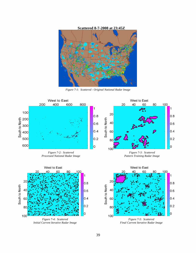
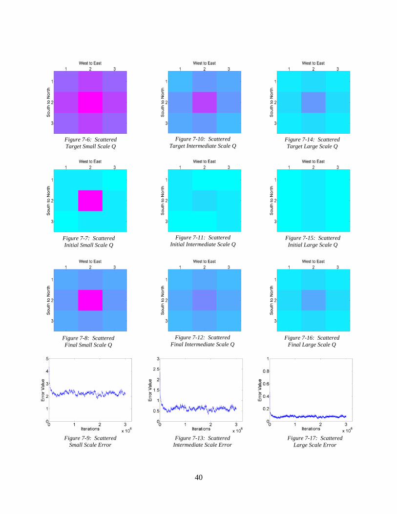
Figure 7-1: Scattered - Original National Radar Image…………………………….…………..39
Figure 7-2: Scattered - Processed National Radar Image…………………………………..…..39
Figure 7-3: Scattered - Pattern Training Radar Image………………………..……….………..39
Figure 7-4: Scattered - Initial Current Iterative Radar Image………………..……….….……..39
Figure 7-5: Scattered - Final Current Iterative Radar Image…………………………...…..…..39
Figure 7-6: Scattered - Target Small Scale Q…………………………………………………..40
Figure 7-7: Scattered - Initial Small Scale Q…………………………….…………..……..…..40
Figure 7-8: Scattered - Final Small Scale Q………………………………………….….....…..40
Figure 7-9: Scattered - Small Scale Error………………………...…………………...………..40
Figure 7-10: Scattered - Target Intermediate Scale Q…………………….………..…………..40
Figure 7-11: Scattered - Initial Intermediate Scale Q…………………………………………..40
Figure 7-12: Scattered - Final Intermediate Scale Q………….……...…………….…….….....40
Figure 7-13: Scattered - Intermediate Scale Error……………………………………….……..40
Figure 7-14: Scattered - Target Large Scale Q…………………………………………..……..40
Figure 7-15: Scattered - Initial Large Scale Q…………………………….…...………...……..40
Figure 7-16: Scattered - Final Large Scale Q……………………...…………………….……..40
Figure 7-17: Scattered - Large Scale Error………………...…………….……………………..40
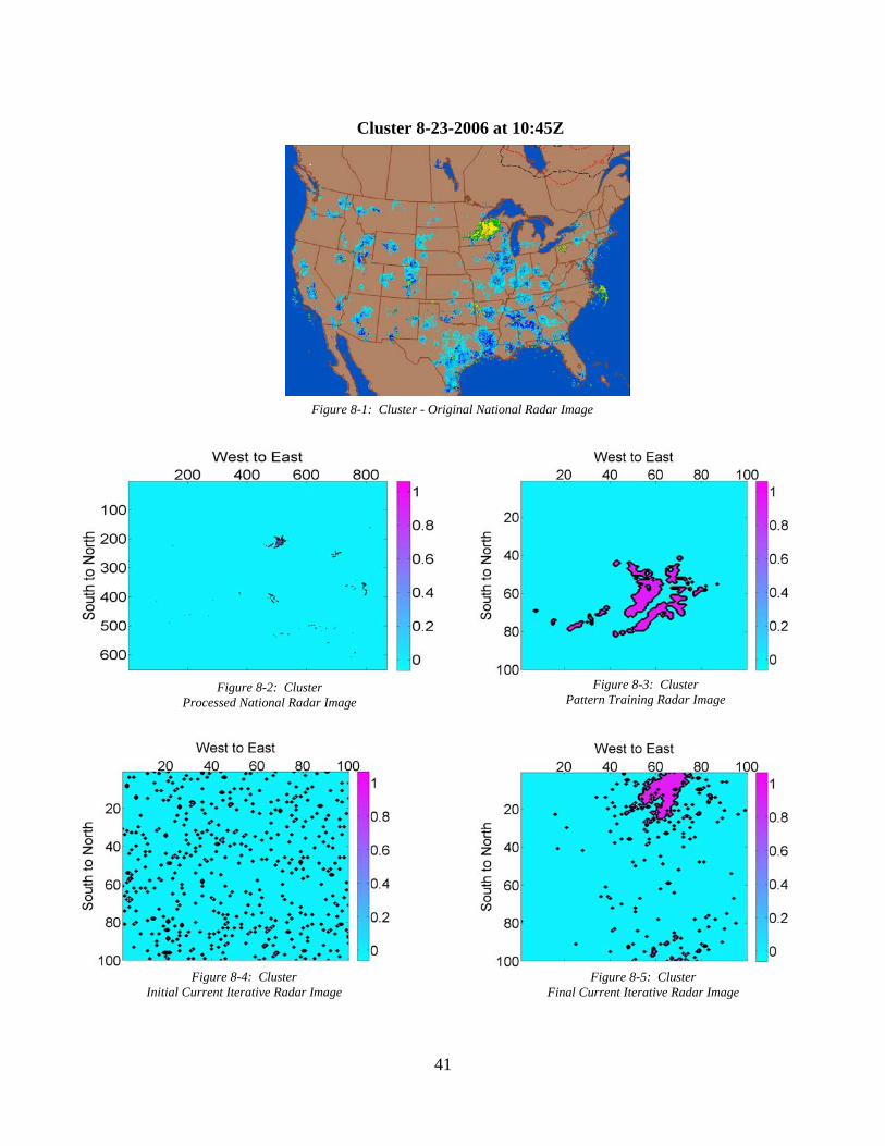
Figure 8-1: Cluster - Original National Radar Image…………………………………………..41
Figure 8-2: Cluster - Processed National Radar Image…………………………….….……….41
Figure 8-3: Cluster - Pattern Training Radar Image………………………………………..…..41
Figure 8-4: Cluster - Initial Current Iterative Radar Image…………….….…………….....…..41
x
LIST OF FIGURES
Figure 8-5: Cluster - Final Current Iterative Radar Image……………………….….……..…..41
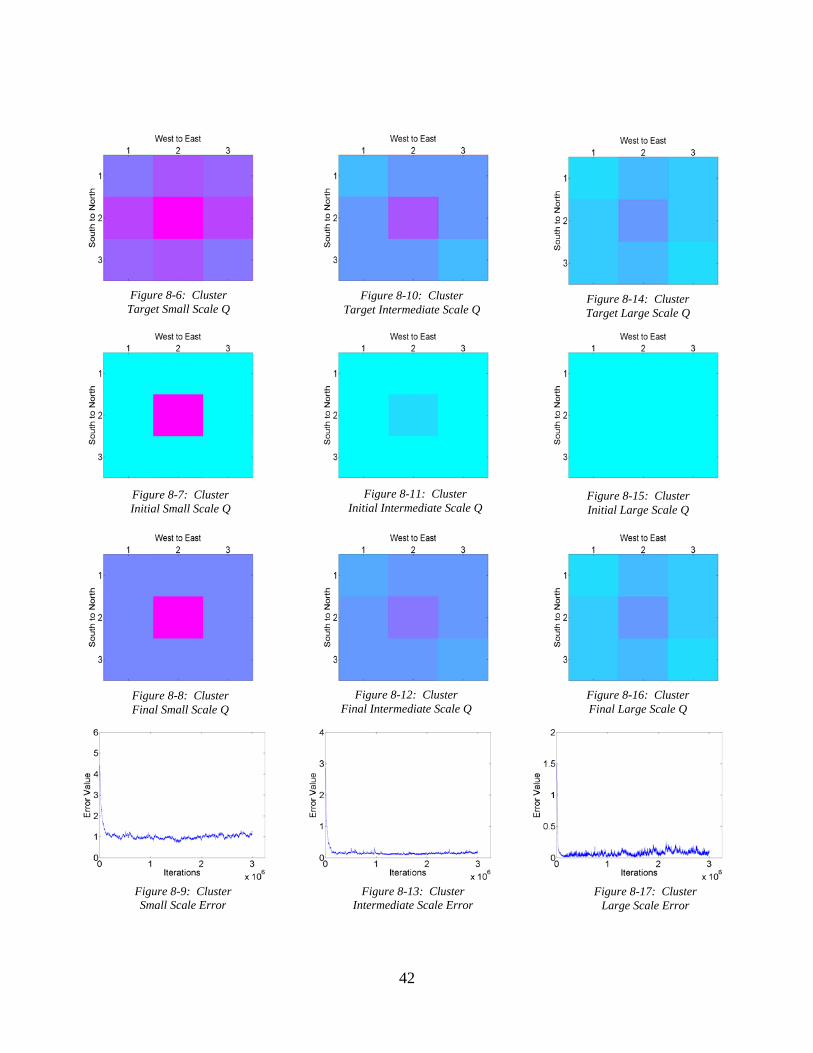
Figure 8-6: Cluster - Target Small Scale Q……………………………...……….……...……..42
Figure 8-7: Cluster - Initial Small Scale Q……………………….……………………...……..42
Figure 8-8: Cluster - Final Small Scale Q………………………...………………….………...42
Figure 8-9: Cluster - Small Scale Error………………………………...……………..………..42
Figure 8-10: Cluster - Target Intermediate Scale Q………………………….………..…….....42
Figure 8-11: Cluster - Initial Intermediate Scale Q………...……………….……………...…..42
Figure 8-12: Cluster - Final Intermediate Scale Q……………...…………….………………..42
Figure 8-13: Cluster - Intermediate Scale Error……………………………....………...….…..42
Figure 8-14: Cluster - Target Large Scale Q………………………………….…...……..….....42
Figure 8-15: Cluster - Initial Large Scale Q……………………………………...…...………..42
Figure 8-16: Cluster - Final Large Scale Q……………………………...……….………...…..42
Figure 8-17: Cluster - Large Scale Error…………………………...…………………………..42

xi
LIST OF ABBREVIATIONS AND NOMENCLATURE
CAPE – Convective Available Potential Energy
CCFP – Collaborative Convective Forecast Product
CIN – Convective Inhibition
FAA – Federal Aviation Administration
GFS – Global Forecast System
LAMP – Localized Aviation Model Output Statistics Product
NEXRAD – Next Generation Radar
Q – Spatial conditional probability map

xii
ACKNOWLEDGEMENTS
I’d like to thank my advisor, George Young, and other committee members, Eugene
Clothiaux and Andrew Kleit, for their support, encouragement, and patience. I’d also like to
thank my family and friends who have provided me with love, strength, and sanity at the most
difficult times. This work was supported under FAA grant number PSU-0001-F800 ATP1 DTD
6/30/09.
1
CHAPTER 1: INTRODUCTION
The Federal Aviation Administration (FAA) is responsible for the safety of civil aviation.
FAA responsibilities include promulgating safety regulations, developing new aviation
technologies, developing and overseeing air traffic control, and regulating commercial air
traffic.1 The traffic flow management performed by the FAA includes a number of tasks.2 The
FAA is responsible for balancing air traffic demand with national air space capacity, while
maintaining maximum utilization of the air space. Air Route Traffic Control Centers work in
conjunction with Terminal Radar Approach Control, which works in conjunction with the
terminal tower, to see that aircraft safely and efficiently traverse routes. Certain rules of thumb
are employed when making decisions regarding air space capacity. The threshold values for
these rules are determined from experience and air traffic simulations using historical weather.
In this effort to oversee air traffic, weather forecasts play a significant role. Snow, ice,
wind, fog, and thunderstorms all create obstacles for pilots. Aircraft flights are often diverted,
delayed, or cancelled due to the impact of weather. Thus, good weather forecasts are necessary
to plan ahead and achieve a stable flow of air traffic through or around weather impediments.
This research project is concerned with improving the convective storm or thunderstorm
forecasts issued by the FAA for air flow management.
The goal of the research is to create a radar image generational algorithm that generates
an ensemble of forecast radar image realizations through combining a forecasted convective
1 What We Do. Federal Aviation Administration. 10 Mar 2010. Web. Feb 2010. <www.faa.gov/about/mission/activitiesl>.
2 Traffic Flow Management in the National Airspace System. Federal Aviation Administration Air Traffic
Organization. Oct 2009. Web. Feb 2010. <http://www.fly.faa.gov/Products/Training/Traffic_Management_for_Pilots/TFM_in_the_NAS_Booklet_ca10.pdf>.
2
probability and quantitative descriptions of the expected two-dimensional convective storm
pattern, referred to as the pattern training radar image spatial conditional probability maps. The
ensemble forecast will provide the FAA with information on the fractional horizontal area the
convective storm will cover, the two-dimensional shape of the convective storm, and the relative
uncertainty associated with the forecast, obtained by comparing the forecast radar images within
the ensemble to each other. The ensemble of forecast radar images will be used by the FAA as
input to drive the Air Traffic Flow Management model. The model output will in turn drive air
traffic flow management strategy. The radar image generational algorithm thus allows the FAA
to have an air traffic flow management strategy prepared less than twenty-four hours in advance
of an expected storm, in an effort to minimize flight delays, flight cancellations, airline costs, and
consumer costs.
Currently, the FAA uses the Collaborative Convective Forecast Product (CCFP) to
forecast convective storms. The CCFP was developed in 1998 and is a product of collaboration
between commercial airline weather offices, business aviation weather offices, and NWS Center
Weather Service Units (CWSUs) located at 20 FAA field offices.3 The collaboration results in a
forecast comprised of three maps: 2 hour, 4 hour, and 6 hour advanced convective forecasts. It is
important to note that the forecast is not necessarily a consensus of opinions. Each of the three
maps depicts shaded areas that reflect convective forecasts containing the categorical expected
probability of thunderstorm occurrence, thunderstorm growth, and top height of thunderstorm
clouds.
The disadvantage of this forecast is that it only forecasts a categorical range for the
3 “The Collaborative Convective Forecast Product (CCFP)”. Collaborative Decision Making. Federal Aviation Administration. 15 Aug 2002. Web. Feb 2010. <http://cdm.fly.faa.gov/Workgroups/WxApps/CCFP%20Information%20Paper%20Aug%2002.doc>.
3
probability of thunderstorm occurrence. The shaded areas within the maps also do not
necessarily reflect the shape of the convection. The shape of the convection is crucial for
deciding whether or not an aircraft should be flown around the convection or if that is impossible
and the aircraft must be flown over or through the convection. Another important disadvantage
of this forecast is its collaborative formulation and unavoidable political implications of specific
airline dominance and airline costs. Thus the CCFP may be purposely skewed by certain
collaborating parties for the narrow interest of those parties.
The radar image generational algorithm seeks to resolve those weaknesses posed by the
current CCFP forecast. In the algorithm, the forecasted convective probability is extracted from
the Localized Aviation Model Output Statistics Product (LAMP), which is derived from the
operational Global Forecast System (GFS). The LAMP forecast provides point forecasts, which
includes a forecast for the probability that convection will occur at a given location. This will
provide the ensemble radar image forecast created by the algorithm with a more specific,
quantitative convective probability rather than the categorical convective probability provided by
the CCFP. Also, the very nature of the ensemble radar image forecast will provide information
about the two-dimensional shape of a storm, a characteristic the CCFP lacks. Lastly, the radar
image generational algorithm is purely objective in its creation of an ensemble of radar image
realizations. The algorithm has no collaborative component prone to subjective influence.
1.1 Summary of Radar Image Generational Algorithm
The radar image generational algorithm combines a spatially varying probabilistic
convective forecast and quantitative descriptions of the expected two-dimensional convective
storm pattern, referred to as the pattern training radar image spatial conditional probability maps,
4
in order to generate an ensemble forecast of radar image realizations. The algorithm generates a
single radar image realization forecast, the current iterative radar image, by iteratively swapping
subsections of pixels within the current iterative radar image until its spatial conditional
probability maps are effectively similar to the corresponding scale of pattern training radar image
spatial conditional probability maps. Similar spatial conditional probability maps indicate that
the radar images from which the spatial conditional probability maps were calculated have
similar two-dimensional convective patterns.
The forecasted convective probability is extracted from LAMP and is interpreted as the
forecasted convective coverage percentage or the fractional area of pixels within a radar image
that are classified as convective pixels. The convective coverage percentage is used to initialize
the algorithm generated radar image realization, the current iterative radar image, by randomly
classifying pixels in the image as convective until the convective coverage fractional number of
pixels is achieved. Every realization within the ensemble of radar image realizations generated
by the algorithm is characterized by having the forecasted convective coverage percentage as the
basis for the number of convective pixels in the radar image.
The second input required, the pattern training radar image spatial conditional probability
maps, are based on an idealized convective pattern as depicted on a real radar image (i.e. front,
squall line, clustered, scattered, or isolated convective pattern). This real radar image is referred
to as the pattern training radar image and its spatial conditional probability maps, conditioned on
a center convective pixel, are required for algorithm input. The pattern training radar image
spatial conditional probability maps provide a quantitative way to compare the pattern training
radar image to the current iterative radar image. The spatial conditional probability maps for a
given radar image are differentiated by different scales or the size of the area of pixels in the
5
radar image that are quantitatively being described by each map. This quantitative comparison is
crucial since the goal of the algorithm is to depict a pattern similar to that of the pattern training
radar image on every radar image realization in the ensemble generated. The patterns on every
realization will not be identical, however, since both the initial pixel positions and the swap
locations are randomly selected. Spatial conditional probability maps are also calculated for the
current iterative radar image and referred to as the current iterative radar image spatial
conditional probability maps.
Once the current iterative radar image spatial conditional probability maps and the pattern
training radar image spatial conditional probability maps are defined, a single variable known as
error is calculated for each identically scaled spatial conditional probability map pair. Error must
be minimized in order to achieve a similar pattern on the current iterative radar image compared
to the pattern training radar image. Error is minimized through the iterative process known as
the swap test. The swap test randomly selects sections of pixels to swap within the current
iterative radar image and recalculates the new error produced by the swap. If the swap
effectively reduces the error, bringing the current iterative radar image pattern closer to the
pattern on the pattern training radar image, then the swap is retained. This process is continued
for millions of iterations.
The resulting current iterative radar image contains a pattern similar to that of the pattern
training radar image and is characterized by the forecasted convective coverage percentage. This
process is repeated to generate each radar image in the ensemble of radar image realizations.
Following the successful development of the algorithm, a statistical analysis is performed
in an effort to automate the selection of the pattern training radar image spatial conditional
probability maps, which is one of the two algorithm inputs. Successful automation is based on
6
finding a well correlated atmospheric variable with the convective pattern categories (i.e. front,
squall line, clustered, scattered, and isolated convection). This is an area that will require future
work.
Once the radar image generational algorithm is successfully automated, several steps
remain to achieve a version of the algorithm fit for FAA convective forecast purposes. This
algorithm generated ensemble of radar image realizations can be used by the FAA to calculate
the likelihood of a given air traffic situation occurring. Anticipating days requiring a reduced
volume of air traffic reduces the strain on the air traffic management system by letting the FAA
prepare in advance.
7
CHAPTER 2: DATA
Observational data are required both as input for the radar image generational algorithm
discussed above and for the statistical analysis used to automate the selection of the appropriate
pattern training radar image spatial conditional probability map. For algorithm input, a
convective coverage percentage and pattern training radar image are required, the latter being
used to create spatial conditional probability maps. For the statistical analysis, sounding data and
surface analysis data are used. In both the algorithm and statistical analysis datasets, actual
observations are used rather than forecasts, making this a “perfect prog” method (Wilks 2006).
The algorithm thus requires two pieces of input data: a convective coverage percentage
and a pattern training radar image. When the algorithm is used to forecast operationally, the
convective coverage percentage will be extracted from the LAMP forecast. In algorithm
development, however, the convective coverage percentage is estimated from the fraction of
convective pixels in the pattern training radar image. In contrast, observed radar images are used
only during development where they are required to create the spatial conditional probability
maps. These maps are then used in the operational forecast process. While we demonstrate the
algorithm using a single radar image to generate each set of spatial conditional probability maps,
one could increase the statistical robustness by averaging the results from several images to
generate each set of spatial conditional probability maps. The algorithm’s task will be easier in
the forecast mode if multiple pattern training radar images with similar convective patterns and
convective coverage percentages are used to generate each set of spatial conditional probability
maps. In forecast mode it would be additionally useful to the algorithm if multiple subsets of
pattern training radar images existed within a group of similar convective patterns (e.g. front
8
segments or clustered convection). Each subset of images would be characterized by similar
convective patterns and convective coverage percentages but the subsets would be differentiated
by the range of convective coverage percentages depicted in the images. The subset containing
the most appropriate convective pattern and having the range of convective coverage percentages
most similar to the convective coverage percentage from the LAMP forecast would be used to
generate a single set of spatial conditional probability maps.
In algorithm development, the pattern training radar images, used to create the spatial
conditional probability maps, are extracted from archived national radar images of the United
States. The archived images were extracted from the Pennsylvania State University Department
of Meteorology e-wall as current radar images and archived.4 The images were produced by
Unidata utilizing 6 km resolution national reflectivity composites measured by the National
Weather Service Next Generation Radar (NEXRAD) network. According to NOAA, the
National Weather Service operates 159 NEXRAD radars, each with a maximum range of 250
nautical miles.5 Each national radar image is composed of 870 pixels by 652 pixels for a total of
567,240 pixels.
In order for a radar image case to be considered for processing in the radar image
generational algorithm, each case is required to pass a manual screening. National radar images
are manually grouped into convective pattern categories and are required to display radar
reflectivities of at least 40 dBZ. The value of 40 dBZ was selected as a relative minimum value
of radar reflectivity for classification of a convective storm. The higher the radar reflectivity, the
4 E-wall: The Electronic Map Wall. The Pennsylvania State University Department of Meteorology. N.d. Web. 2006-2008. <http://www.meteo.psu.edu/ewall/ewall.html>.
5 “About the Radar Operations Center.” NOAA’s National Weather Service Radar Operations Center.
9 Feb 2010. Web. Feb 2010. < http://www.roc.noaa.gov/WSR88D/About.aspx>.
9
larger the size of precipitation particles and thus, the stronger the associated storm updraft, both
of which can be dangerous to aircraft. The convective pattern categories are clustered
convection, isolated convection, front segment, squall line, or scattered convection. Not all cases
that fall into these categories are processed however. The number of cases processed from each
category is relatively equivalent: 8 fronts, 8 clustered, 8 isolated, 8 scattered, and 9 squall lines.
So only a select number of cases are processed. The 41 cases selected for processing in the radar
image generational algorithm are predominantly from May through September 2006 but there are
a few from May through September 2008.
In order to complete the statistical analysis required to find a variable well correlated with
the convective pattern categories and thus automate the selection of the appropriate set of spatial
conditional probability maps, atmospheric sounding data and surface front analysis data
associated with each case is used. The cases incorporated in the statistical analysis include those
41 cases previously used for processing by the algorithm in addition to 147 new cases. New
cases are identified using the same national radar image and convective pattern categorization as
described above. The only difference between the algorithm processed cases and the new cases
is that the former are processed by the algorithm and a radar image forecast has been generated
while the latter have not been processed and do not have a radar image forecast associated with
them. This difference, however, is irrelevant for the purposes of the statistical analysis. The new
cases are from May through September 2007 exclusively. For each of the new cases the
associated sounding data and surface analyses are recorded. Thus a total of 188 possible cases
are available for use in the statistical analysis. Not all these cases, however, are employed in the
final statistical analysis presented in the results chapter.
10
The sounding data utilized in the statistical analysis to automate the selection of the set of
spatial conditional probability maps, is downloaded from the University of Wyoming
atmospheric sounding site.6 Sounding data is measured through the National Weather Service
Upper-Air Observations Program using radiosondes. As of January 2010, 102 radiosonde
stations are operational in North America, the Pacific Islands, and the Caribbean. Soundings are
conducted by the National Weather Service and normally are taken twice a day at 00 Z and 12 Z,
365 days a year. Radiosonde measurements include pressure, temperature, and relative humidity
profiles, together with derived wind speed and direction from GPS tracking. All other variables
listed on a sounding are calculated from these profiles.7
The sounding recorded for each case is generally south to southeast of the specific
convective storm, where the source of storm moisture is generally located. Since soundings are
only available in 12 hour increments, the sounding recorded for each case is required to occur
prior to the radar image time stamp. This was done in an effort to ensure that pre-storm
atmospheric conditions or the atmospheric characteristics of the air feeding into the storm are
recorded, not the post-storm atmospheric variables. Sounding data extracted for use in the
statistical analysis includes the K-index, convective available potential energy (CAPE),
convective inhibition (CIN), and wind speed and direction from the surface, 3000 m level, and
6000 m level. Note that these levels were used based on flight level standards in forecasts issued
by the FAA.
6 Upper Air Sounding. University of Wyoming College of Engineering Department of Atmospheric Science. N.d. web. Feb 2010. < http://weather.uwyo.edu/upperair/sounding.html>.
7 “What is a radiosonde?” National Weather Service Radiosonde Observations. National Weather
Service. N.d. web. Feb 2010. <http://www.ua.nws.noaa.gov/factsheet.htm>.
11
The statistical analysis required to automate the selection of the set of spatial conditional
probability maps also incorporates surface analyses, containing information on the presence of
fronts. Surface analyses are obtained from the Hydrometeorological Prediction Center (HPC).8
Analyses are issued in 3 hour time intervals and depict surface synoptic and mesoscale features
such as high and low pressure systems, fronts, troughs, outflow boundaries, squall lines and dry
lines. The analyses include most of North America and its bordering oceans.9 The surface
analysis used in each case is the most recent surface analysis occurring prior to the radar image
time stamp. In order for a stationary or cold front on a surface analysis to be associated with
convection occurring in a case, the front must occur within 600 km of the convection, measured
perpendicular to the front. This distance was judged to be a fair assessment of whether or not a
front is in the vicinity of the convection.
The radar image data in the radar image generational algorithm and sounding data and
surface analyses in the statistical analysis are screened for completeness and errors. National
radar images containing questionable reflectivity values are omitted and so are any associated
cases. Atmospheric soundings containing incomplete information are omitted and replaced with
substitute soundings from the same day and time but at an alternate sounding location. Surface
analyses are examined for completeness but none are found deficient.
8 HPC’s Surface Analysis Archive. Hydrometeorological Prediction Center. 1 Mar 2007. Web. Feb 2010. <http://www.hpc.ncep.noaa.gov/html/sfc_archive.shtml>.
9 About the Surface Analysis. Hydrometeorological Prediction Center. 1 Mar 2007. Web. Feb 2010.
<http://www.hpc.ncep.noaa.gov/html/about_sfc.shtml>.
12
CHAPTER 3: PROCEDURES
As previously explained, the FAA convective forecast is concerned with how convective
coverage translates into air space capacity within an air traffic sector. The goal of the radar
image generational algorithm is to combine a convective coverage percentage forecast with a
pattern training radar image to generate an ensemble of radar image realizations. This is
achieved over a series of iterations, where the set of spatial conditional probability maps of the
pattern training radar image will be compared to the set of spatial conditional probability maps of
the current iterative radar image at each scale, as the latter is altered to appear similar to the
former. The current iterative radar image is altered by randomly selecting sections of pixels and
swapping them until the set number of iterations is achieved. Upon completion, the current
iterative radar image will be characterized by the convective coverage percentage forecast and a
convective pattern similar to that depicted on the pattern training radar image, as described by
the similar spatial conditional probability map sets. If this iteration process is run repeatedly the
algorithm output takes the form of an ensemble of radar image realizations, although currently
the algorithm output is only a single radar realization. Operationally, the ensemble of radar
realizations would then be used in conjunction with the air traffic modeling software to assess
the impact of convective storms on the air traffic capacity. The availability of multiple radar
realizations also will give an indication of the convective forecast uncertainty.
3.1 Radar Image Generational Algorithm Inputs
The convective coverage percentage forecast, one of the two radar image generational
algorithm inputs, will be derived from the LAMP forecast when the algorithm is forecasting
13
operationally. LAMP provides a forecast for the probability that convection will occur at given
gridded locations. In order to use the LAMP probability grid, an assumption must be made. It is
assumed that within a radar image forecast area, the average of the point forecast probabilities
provided by LAMP is equivalent to the fractional amount of the land area that is covered with
convection at the forecast time. For example, in a 5 pixel by 5 pixel radar image, an average
LAMP probability of 20% would translate to 5 of the 25 pixels being defined as convective. The
disadvantage of this assumption is that it is not completely accurate. In reality, converting the
LAMP convective probability grid to a fractional area coverage will require recalibration, likely
using linear regression. As previously explained, for developmental purposes, the convective
coverage percentage is estimated from the fractional convective coverage area depicted in the
pattern training radar image.
The second algorithm input, the pattern training radar image, is derived from real radar
images. Its purpose is to provide information about the size and shape of a convective storm,
which is required to calculate the spatial conditional probability maps used as a goal standard of
comparison throughout the algorithm iterations. The real national radar images are read in by the
algorithm and all radar reflectivities 40 dBZ and greater are interpreted as convective pixels.
Reflectivities less than 40 dBZ are interpreted as non-convective pixels. A two-dimensional
matrix of ones and zeros is used to represent the original radar image depicting the pattern of the
storm. Ones represent convective pixels in a radar image and zeros represent non-convective
pixels. This two-dimensional matrix representing a convective radar pattern is known as the
pattern training radar image.
14
3.2 The Current Iterative Radar Image
In order to combine the convective coverage percentage and the pattern training radar
image, a hypothetical radar map known as the current iterative radar image is created. The
current iterative radar image, containing the forecasted convective coverage percentage,
rearranges randomly located convective pixels into a pattern similar to the pattern on the pattern
training radar image through many iterations of swapping subsections of pixels within the
current iterative radar image. The final version of the current iterative radar image is a single
radar realization among the multiple radar realizations necessary to create an ensemble of radar
realizations.
The current iterative radar image is initialized utilizing the convective coverage
percentage. Using the assumption that a point probability of convection is equivalent to the
fractional land coverage of convection, a two-dimensional matrix is created to represent the
forecast area. This matrix is called the current iterative radar image. It is equivalent in size to
the matrix used for the pattern training radar image. As in the case of the pattern training radar
image, ones again represent convective pixels and zeros represent non-convective pixels. The
cells or pixels in the current iterative radar image are randomly assigned a value of one until a
fractional number of the pixels is equivalent to the convective coverage percentage. The
remaining unassigned pixels are assigned a value of zero.
3.3 Spatial Conditional Probability
In order to bring randomly assigned convective pixels in the current iterative radar image
into a convective pattern resembling that in the pattern training radar image, a quantitative means
of comparing the current iterative radar image to the pattern training radar image is required.
15
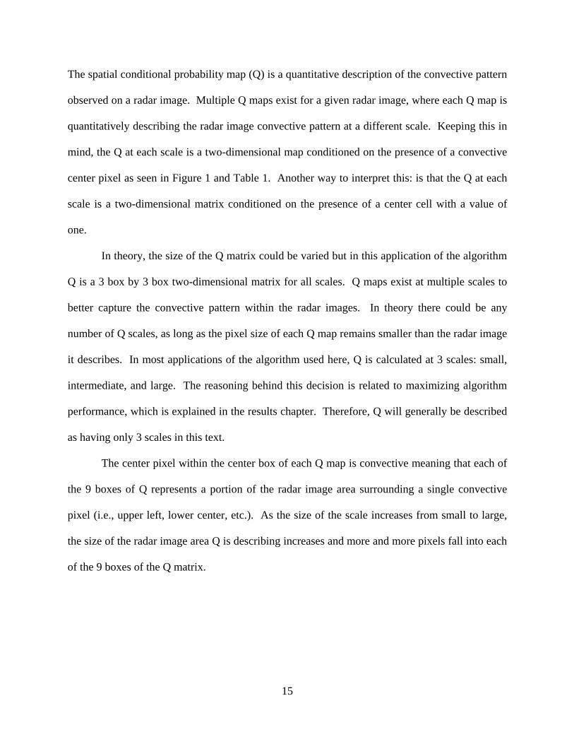
The spatial conditional probability map (Q) is a quantitative description of the convective pattern
observed on a radar image. Multiple Q maps exist for a given radar image, where each Q map is
quantitatively describing the radar image convective pattern at a different scale. Keeping this in
mind, the Q at each scale is a two-dimensional map conditioned on the presence of a convective
center pixel as seen in Figure 1 and Table 1. Another way to interpret this: is that the Q at each
scale is a two-dimensional matrix conditioned on the presence of a center cell with a value of
one.
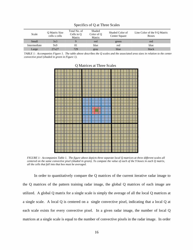
In theory, the size of the Q matrix could be varied but in this application of the algorithm
Q is a 3 box by 3 box two-dimensional matrix for all scales. Q maps exist at multiple scales to
better capture the convective pattern within the radar images. In theory there could be any
number of Q scales, as long as the pixel size of each Q map remains smaller than the radar image
it describes. In most applications of the algorithm used here, Q is calculated at 3 scales: small,
intermediate, and large. The reasoning behind this decision is related to maximizing algorithm
performance, which is explained in the results chapter. Therefore, Q will generally be described
as having only 3 scales in this text.
The center pixel within the center box of each Q map is convective meaning that each of
the 9 boxes of Q represents a portion of the radar image area surrounding a single convective
pixel (i.e., upper left, lower center, etc.). As the size of the scale increases from small to large,
the size of the radar image area Q is describing increases and more and more pixels fall into each
of the 9 boxes of the Q matrix.
16
In order to quantitatively compare the Q matrices of the current iterative radar image to
the Q matrices of the pattern training radar image, the global Q matrices of each image are
utilized. A global Q matrix for a single scale is simply the average of all the local Q matrices at
a single scale. A local Q is centered on a single convective pixel, indicating that a local Q at
each scale exists for every convective pixel. In a given radar image, the number of local Q
matrices at a single scale is equal to the number of convective pixels in the radar image. In order
Q Matrices at Three Scales
FIGURE 1: Accompanies Table 1. The figure above depicts three separate local Q matrices at three different scales allcentered on the same convective pixel (shaded in green). To compute the value of each of the 9 boxes in each Q matrix,all the cells that fall into that box must be averaged.
TABLE 1: Accompanies Figure 1. The table above describes the Q scales and the associated area sizes in relation to the centerconvective pixel (shaded in green in Figure 1).
Specifics of Q at Three Scales
Scale Q Matrix Size cells x cells
Total No. of Cells in Q
Matrix
Shaded Color of Q
Matrix
Shaded Color of Center Square
Line Color of the 9 Q Matrix Boxes
Small 3x3 9 red green red Intermediate 9x9 81 blue red blue
Large 27x27 729 gray blue black
17
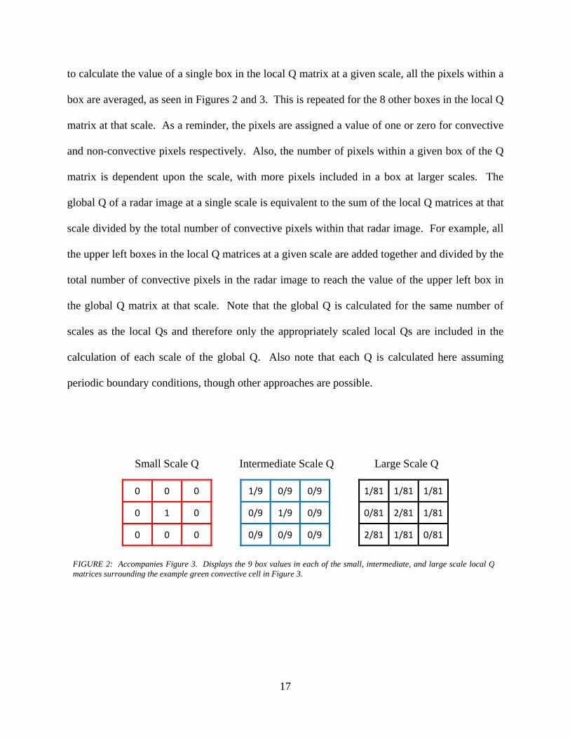
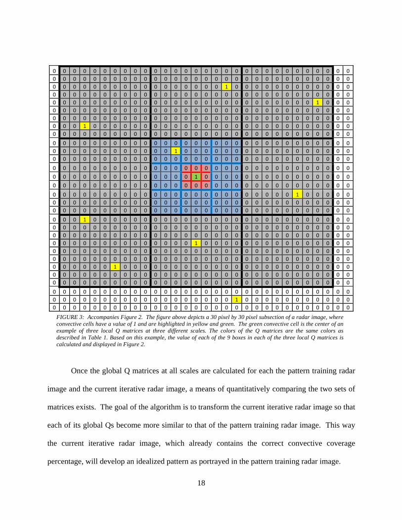
to calculate the value of a single box in the local Q matrix at a given scale, all the pixels within a
box are averaged, as seen in Figures 2 and 3. This is repeated for the 8 other boxes in the local Q
matrix at that scale. As a reminder, the pixels are assigned a value of one or zero for convective
and non-convective pixels respectively. Also, the number of pixels within a given box of the Q
matrix is dependent upon the scale, with more pixels included in a box at larger scales. The
global Q of a radar image at a single scale is equivalent to the sum of the local Q matrices at that
scale divided by the total number of convective pixels within that radar image. For example, all
the upper left boxes in the local Q matrices at a given scale are added together and divided by the
total number of convective pixels in the radar image to reach the value of the upper left box in
the global Q matrix at that scale. Note that the global Q is calculated for the same number of
scales as the local Qs and therefore only the appropriately scaled local Qs are included in the
calculation of each scale of the global Q. Also note that each Q is calculated here assuming
periodic boundary conditions, though other approaches are possible.
0 0 0 1/9 0/9 0/9 1/81 1/81 1/81
0 1 0 0/9 1/9 0/9 0/81 2/81 1/81
0 0 0 0/9 0/9 0/9 2/81 1/81 0/81
Large Scale Q Intermediate Scale Q Small Scale Q
FIGURE 2: Accompanies Figure 3. Displays the 9 box values in each of the small, intermediate, and large scale local Qmatrices surrounding the example green convective cell in Figure 3.
18
0 0 0 0 0 0 0 0 0 0 0 0 0 0 0 0 0 0 0 0 0 0 0 0 0 0 0 0 0 0 0 0 0 0 0 0 0 0 0 0 0 0 0 0 0 0 0 0 0 0 0 0 0 0 0 0 0 0 0 0 0 0 0 0 0 0 0 0 0 0 0 0 0 0 0 0 0 1 0 0 0 0 0 0 0 0 0 0 0 0 0 0 0 0 0 0 0 0 0 0 0 0 0 0 0 0 0 0 0 0 0 0 0 0 0 0 0 0 0 0 0 0 0 0 0 0 0 0 0 0 0 0 0 0 0 0 0 0 0 0 0 0 0 0 0 0 1 0 0 0 0 0 0 0 0 0 0 0 0 0 0 0 0 0 0 0 0 0 0 0 0 0 0 0 0 0 0 0 0 0 0 0 0 0 0 0 0 0 0 0 0 0 0 0 0 0 0 0 0 0 0 0 0 0 0 0 0 0 0 0 0 0 0 1 0 0 0 0 0 0 0 0 0 0 0 0 0 0 0 0 0 0 0 0 0 0 0 0 0 0 0 0 0 0 0 0 0 0 0 0 0 0 0 0 0 0 0 0 0 0 0 0 0 0 0 0 0 0 0 0
0 0 0 0 0 0 0 0 0 0 0 0 0 0 0 0 0 0 0 0 0 0 0 0 0 0 0 0 0 0 0 0 0 0 0 0 0 0 0 0 0 0 1 0 0 0 0 0 0 0 0 0 0 0 0 0 0 0 0 0 0 0 0 0 0 0 0 0 0 0 0 0 0 0 0 0 0 0 0 0 0 0 0 0 0 0 0 0 0 0
0 0 0 0 0 0 0 0 0 0 0 0 0 0 0 0 0 0 0 0 0 0 0 0 0 0 0 0 0 0
0 0 0 0 0 0 0 0 0 0 0 0 0 0 1 0 0 0 0 0 0 0 0 0 0 0 0 0 0 0
0 0 0 0 0 0 0 0 0 0 0 0 0 0 0 0 0 0 0 0 0 0 0 0 0 0 0 0 0 0
0 0 0 0 0 0 0 0 0 0 0 0 0 0 0 0 0 0 0 0 0 0 0 0 1 0 0 0 0 0 0 0 0 0 0 0 0 0 0 0 0 0 0 0 0 0 0 0 0 0 0 0 0 0 0 0 0 0 0 0 0 0 0 0 0 0 0 0 0 0 0 0 0 0 0 0 0 0 0 0 0 0 0 0 0 0 0 0 0 0
0 0 0 1 0 0 0 0 0 0 0 0 0 0 0 0 0 0 0 0 0 0 0 0 0 0 0 0 0 0 0 0 0 0 0 0 0 0 0 0 0 0 0 0 0 0 0 0 0 0 0 0 0 0 0 0 0 0 0 0 0 0 0 0 0 0 0 0 0 0 0 0 0 0 0 0 0 0 0 0 0 0 0 0 0 0 0 0 0 0 0 0 0 0 0 0 0 0 0 0 0 0 0 0 1 0 0 0 0 0 0 0 0 0 0 0 0 0 0 0 0 0 0 0 0 0 0 0 0 0 0 0 0 0 0 0 0 0 0 0 0 0 0 0 0 0 0 0 0 0 0 0 0 0 0 0 0 0 0 0 0 0 0 0 0 0 0 0 0 0 0 0 0 0 0 0 0 0 0 0 0 0 0 0 0 0 1 0 0 0 0 0 0 0 0 0 0 0 0 0 0 0 0 0 0 0 0 0 0 0 0 0 0 0 0 0 0 0 0 0 0 0 0 0 0 0 0 0 0 0 0 0 0 0 0 0 0 0 0 0 0 0 0 0 0 0 0 0 0 0 0 0 0 0 0 0 0 0 0 0 0 0 0 0 0 0 0 0 0 0
0 0 0 0 0 0 0 0 0 0 0 0 0 0 0 0 0 0 0 0 0 0 0 0 0 0 0 0 0 0 0 0 0 0 0 0 0 0 0 0 0 0 0 0 0 0 0 0 1 0 0 0 0 0 0 0 0 0 0 0 0 0 0 0 0 0 0 0 0 0 0 0 0 0 0 0 0 0 0 0 0 0 0 0 0 0 0 0 0 0
Once the global Q matrices at all scales are calculated for each the pattern training radar
image and the current iterative radar image, a means of quantitatively comparing the two sets of
matrices exists. The goal of the algorithm is to transform the current iterative radar image so that
each of its global Qs become more similar to that of the pattern training radar image. This way
the current iterative radar image, which already contains the correct convective coverage
percentage, will develop an idealized pattern as portrayed in the pattern training radar image.
FIGURE 3: Accompanies Figure 2. The figure above depicts a 30 pixel by 30 pixel subsection of a radar image, whereconvective cells have a value of 1 and are highlighted in yellow and green. The green convective cell is the center of anexample of three local Q matrices at three different scales. The colors of the Q matrices are the same colors asdescribed in Table 1. Based on this example, the value of each of the 9 boxes in each of the three local Q matrices iscalculated and displayed in Figure 2.
19
3.4 The Swap Test
The swap test is the iterative portion of the algorithm. It repeatedly swaps subsections of
pixels in the current iterative radar image with other subsections within the same image. The
goal of the swap test is to bring the randomly assigned convection in the current iterative radar
image into a coherent pattern resembling that in the pattern training radar image. It does this by
comparing the global Q matrices of the two radar images after every swap to assess if at a given
scale the Q matrix of the current iterative radar image is more similar to the target Q of the
pattern training radar image. This verification process is the swap test.
Error is the means of quantitatively comparing the global Q matrices of the current
iterative radar image and the pattern training radar image at a single scale. As in the case of the
global Q matrices, error also exists at multiple scales. The equation for error at a single scale is:
Equation (1)
, ,
Equation 1 indicates that error is always non-negative. The larger the error value, the more
dissimilar the Q matrices and associated radar images are. An error value of zero indicates that
the two Qs are identical at that scale. In theory, if the error value at each and every scale is zero,
the current iterative radar image and the pattern training radar image have identical patterns, but
the feature location is free to vary due to the periodic boundary conditions used to calculate the
Q matrices. However, an error value of zero is unlikely to ever occur on the scale of radar
images with tens of thousands of pixels.
Next, in order to iteratively swap subsections of the current iterative radar image,
specifications concerning the swap must be designated. Specifically, the location and size of the
20
area being swapped must be indicated. Two pixel locations within the current iterative radar
map are randomly selected and identified as pixel 1 and pixel 2. The zero or one value of the
pixels is irrelevant. A Q scale is also randomly selected from among small, intermediate, and
large scales. The Q matrices have boxes containing a varying number of pixels with larger
scaled boxes containing more pixels as seen in Table 1. The pixel size of a single box is
important because it designates the size of the swap-able area surrounding the randomly chosen
pixels. If specifically scaled Q matrix overlays are centered over each of the randomly selected
pixel 1 and pixel 2 locations, all the pixels included in the center box of the Q matrix are
included in the swap. More specifically, pixels contained in the center box of the Q matrix
centered on pixel 1 are swapped with the pixels contained in the center box of the Q matrix
centered on pixel 2.
After a swap has been executed it is necessary to assess if the swap decreased the error
measurement at the scale randomly designated for the swap. A decreased error value indicates
that the change in the global Q matrix of the current iterative radar image was an adjustment that
brought it closer to the global Q matrix of the pattern training radar image. Since this is the goal
of the swap test, only those swaps that cause a decrease in the error value at the selected scale are
retained. Swaps that do not meet the criteria are reversed and new random specifications are
selected. For retained swaps, several variables are updated as well. The global Q matrix of the
current iterative radar image must be calculated for the other scales that were not randomly
chosen for comparison use in the swap test. Also, the associated errors for other scales must be
calculated.
The swap test is repeated for a set number of iterations as defined by the user. The
number of iterations necessary depends upon the pixel grid size and convective coverage
21
percentage of the radar image being processed. An ideal number of iterations will illustrate an
error value that asymptotes as the number of iterations increases. Of course squandering
computer resources is undesirable and the number of iterations that can be used are limited. The
number of iterations utilized in development is discussed in the results chapter.
It is important to note that in order for a swap to be accepted and retained, only the error
at a single scale, the randomly selected scale, is required to decrease. The errors at the other
scales may increase or decrease. They are irrelevant to the acceptance of a swap. Although by
randomly addressing all of the scales, it is hoped that all three errors are driven down by the end
of the iterative process. It is known from conducted algorithm runs, that only requiring one of
the scales of error to decrease, minimizes error more efficiently and avoids local minima of error,
as opposed to requiring all three scales of error to decrease in order to retain a swap.
3.5 Statistical Analysis Methods
The radar image generational algorithm, at this point, is not automated for the selection of
the pattern training radar image and its associated spatial conditional probability maps. It is
hypothesized, however, that certain atmospheric variables are likely indicative of the type of
convective storm pattern. If the algorithm were to utilize forecasts of atmospheric variables well
correlated with the convective storm pattern, it would allow for automated selection of the spatial
conditional probability maps by the algorithm. A statistical analysis is performed to find
atmospheric variables that are well correlated with specific convective pattern categories. The
convective pattern categories are scattered convection, isolated convection, clustered convection,
squall lines, and front segments. The atmospheric variables of interest are the K-index,
Convective Available Potential Energy (CAPE), Convective Inhibition (CIN), the presence or
22
absence of a front in the vicinity, and wind shear from the surface to 3000 m, 3000 m to 6000 m,
and the surface to 6000 m. These variables are indicators of storm moisture, energy, shear
strength, and shear direction, which all influence a convective storm pattern. A total of 188
cases are included in the statistical analysis database.
The first step of the analysis is to manually classify the convective pattern category of
each of the 188 cases.
• Front segment: subsection of a larger front associated with a low pressure system,
visible on a national or regional scale.
• Squall line: a pattern of short linear convection not adjacent to any apparent front.
• Isolated convection: one to a few convective cells in an area largely devoid of
connective activity.
• Scattered convection: multiple cells of convection randomly distributed throughout a
wide area in no apparent pattern.
• Clustered convection: multiple cells of convection in close proximity and lacking a
linear structure to the convective pattern.
Upon completion of the manual analysis, atmospheric variable data are recorded for each
case as described in the data chapter. The K-index, CAPE, CIN, surface wind speed and
direction, 3000 m wind speed and direction, and 6000 m wind speed and direction are collected
from associated upper air soundings. The presence of a cold or stationary front in the vicinity of
the convection of interest is recorded utilizing HPC surface analyses. Shear in the u and v wind
components, wind shear magnitude, and wind shear direction are calculated at three levels: the
surface to 3000 m, 3000 m to 6000 m, and the surface to 6000 m.
23
Two statistical approaches are utilized in an effort to find the atmospheric variable(s) that
are needed to correctly classify the highest percentage of cases based on the five convective
pattern category classifications. First, cluster analysis in Matlab is explored and then the
regression analyses in Weka (Witten and Frank 2005) are explored. Also, instead of only
calculating the percentage of correctly classified cases based on the five convective pattern
category classifications, the convective pattern category classifications can be simplified. The
convective pattern categories are divided into two groups of convective pattern types: linearly
organized convective patterns and randomly organized convective patterns. Random convective
patterns include isolated convection, scattered convection, and clustered convection. Linear
convective patterns include front segments and squall lines. This simplistic approach is logical
because the three classes of random convection are only differentiated by the fractional coverage
of convection. Isolated convection covers the least area, scattered covers an intermediate area,
and clustered convection covers the most area but all three are randomly organized. The linearly
organized convection on the other hand is often indistinguishable on a 100 pixel by 100 pixel
scale. In either case, if the algorithm were successful in selecting the random or linear type of
pattern training radar image, it only requires the convective coverage percentage to narrow down
which type of random classification the case falls into if the algorithm selects the random type.
It doesn’t need to distinguish squall lines and fronts at all for purposes of producing 100 pixel by
100 pixel radar images.
So if the atmospheric variables do not correctly classify cases based on the five
convective pattern categories, a simpler approach using the two convective pattern types can also
be explored. The simpler approach has the possibility of achieving a higher percentage of
correctly classified cases based on the two convective pattern types rather than the five
24
convective pattern categories. The higher the percentage of cases correctly classified, the more
accurately the algorithm will be able to forecast the appropriate set of spatial conditional
probability maps. This is crucial to creating a useful, autonomous algorithm.
25
CHAPTER 4: RESULTS
The radar image generational algorithm successfully combines a convective coverage
percentage forecast with a pattern training radar image to generate an ensemble of radar image
realizations when both synthetic and real radar images are used to create the pattern training
spatial conditional probability maps. The algorithm, however, displays both strengths and
weaknesses in its ability to resolve certain convective pattern characteristics and successful use
of the algorithm is stipulated by certain Q-scale size and swap test repetition requirements.
Overall, the generated radar image realizations display the correct convective coverage
percentage and a pattern similar to that displayed on the pattern training radar image.
The statistical analysis necessary to automate the selection of the pattern training spatial
conditional probability maps through correlating atmospheric variables with convective pattern
categories, is less successful. Weka regression analysis became the preferred statistical analysis
tool over Matlab cluster analysis but the percentage of correctly classified cases that the
atmospheric variables achieve based on the five convective pattern categories is poor even in
Weka. The simpler method of using two convective pattern types instead of five convective
pattern categories is more successful but this is an area that will require future work.
4.1 Radar Image Generational Algorithm Stipulations
In order to successfully utilize the radar image generational algorithm, stipulations
concerning the minimum size of the largest Q scale and minimum number of swap test iterations
must be met. The number of swap test iterations dictates the degree to which the Q matrices of
the current iterative radar image can be altered to appear similar to the corresponding Q matrices
26
of the pattern training radar image. This is important because the goal of the algorithm is to
make these two sets of Q matrices as similar as possible at each scale. The size of the largest Q
scale dictates the largest scale at which the algorithm can “see” the convective pattern. Wider
convective patterns will need a larger size for the largest Q scale in order for the algorithm to
perceive the large scale width and correctly resolve the pattern.
As discussed in the procedures chapter, the number of iterations dictates how many
iterations of the swap test are performed. The swap test is the process of comparing the
corresponding Q matrices of the pattern training radar image and the current iterative radar
image before and after swapping a section of pixels in the current iterative radar image. If the
error, the quantitative difference between two Q matrices at the same scale, decreases, then the
swap is retained. The minimum number of iterations must depict an error that asymptotes as the
number of iterations increases. This illustrates that the pairs of Q matrices at the same scale have
become as similar as they reasonably can, which is the goal of the swap test.
When using 100 pixel by 100 pixel radar images, as is done in algorithm development,
the number of iterations required is between 1 million and 10 million, depending on the
convective coverage percentage. A higher convective coverage percentage will require a larger
number of iterations to successfully resolve the current iterative radar image. A benchmark of 3
million iterations is used during algorithm development, in order to develop a standard of
comparison. The algorithm is able to successfully resolve the majority of the 41 test cases at this
level.
The second stipulation for successful use of the radar image generational algorithm, is
that the largest sized Q scale must meet a minimum threshold, so the algorithm can “see” the
largest convective pattern. As explained in the procedures chapter, during the swap test, a
27
random scale of Q is selected. This random Q scale determines the size in pixels of the
swappable areas in the current iterative radar image. The size of the center box of the random Q
scale is the size of the two areas swapped. In order for the algorithm to accurately resolve the
convection, it must “see” the largest scale of the convection. The bandwidth10 is the width of the
narrowest axis of the convective pattern depicted in the pattern training radar image. The
algorithm must be able to perceive the width of the bandwidth, in order to correctly depict the
convective pattern as an unbroken, continuous pattern, if that is the case. So the size of the
center box at the largest Q scale, must be slightly less than or equal to the size of the bandwidth.
This can be seen in Table 2.
Table 2 lists 4 possible scale sizes and the size of the center box of Q at each of those
scales. For each scale, 4 different algorithm runs are conducted, where different simulated
convective patterns are used for the pattern training radar image. The simulated convective
patterns are differentiated by having bandwidths of sizes 1, 3, 7, and 25. For a given scale, the
algorithm is best able to resolve the pattern that has a bandwidth most similar to the size of the
center box at that scale. Thus, the size of the center box of the largest Q scale must be slightly
less than or equal to the size of the pattern bandwidth depicted in the pattern training radar
image.
10 This is the width of the convective band, not to be confused with the definition used in the signal processing literature.
TABLE 2: Bandwidth, the width of the narrowest axis of the convective pattern in the pattern training radar image, must beslightly less than or equal to the size of the center box of Q.
Q Size Requirements of Correctly Calibrated Algorithm Scale Size Number (Small to Large) 1 2 3 4 Size of Center Box (no. pixels x no. pixels) 1x1 3x3 9x9 27x27
Bandwidth Size With Best Algorithm Results (Possible Bandwidths: 1, 3, 7, 25 ) 1 1 & 3 7 25
28
In algorithm development, the largest scale size is set to 3, the “large” scale described in
Table 1. This benchmark is set to allow for a standard of comparison. A scale of 3 is chosen
because it is the largest scale necessary out of the 41 cases the algorithm processed from 100
pixel by 100 pixel pattern training radar images.
4.2 Radar Image Generational Algorithm Strengths and Weaknesses
The radar image generational algorithm displays both strengths and weaknesses in its
ability to evolve the pattern in the current iterative radar image into a pattern similar to that in the
pattern training radar image. This is a direct reflection of the effectiveness of using the spatial
conditional probability maps as a means to quantitatively compare the convective pattern on the
pattern training radar image to the convective pattern on the current iterative radar image. The
algorithm strengths, however, outweigh the algorithm weaknesses. The algorithm strengths and
weaknesses are best illustrated with the assistance of example cases. The graphics from example
cases are followed by a discussion of the algorithm strengths and weaknesses.
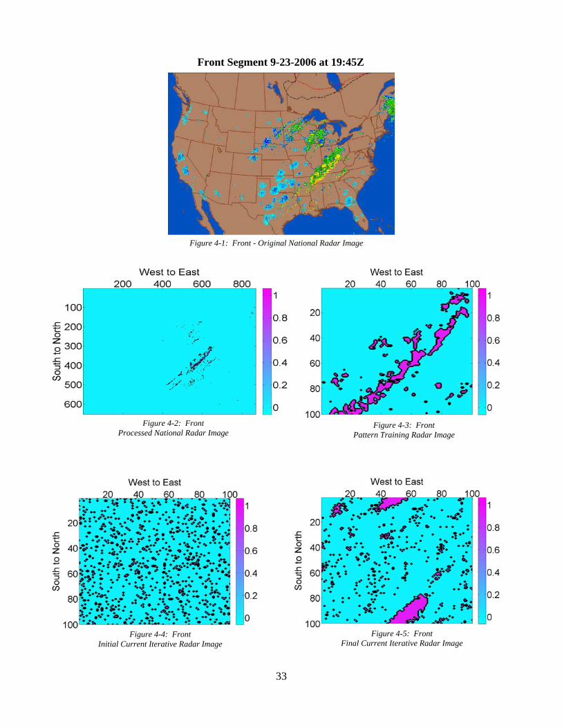
Five example algorithm processed cases are displayed as follows, one from each
convective pattern category: front segment, squall line, isolated convection, scattered convection,
and clustered convection. The front segment case is from September 23, 2006, at 19:45 Z. The
squall line case is from August 13, 2006, at 21:45 Z. The isolated convection case is from June
19, 2006, at 19:45 Z. The scattered convection case is from August 7, 2008, at 23:45 Z. The
clustered convection case is from August 23, 2006, at 10:45 Z. The image panel for each case is
composed of:

29
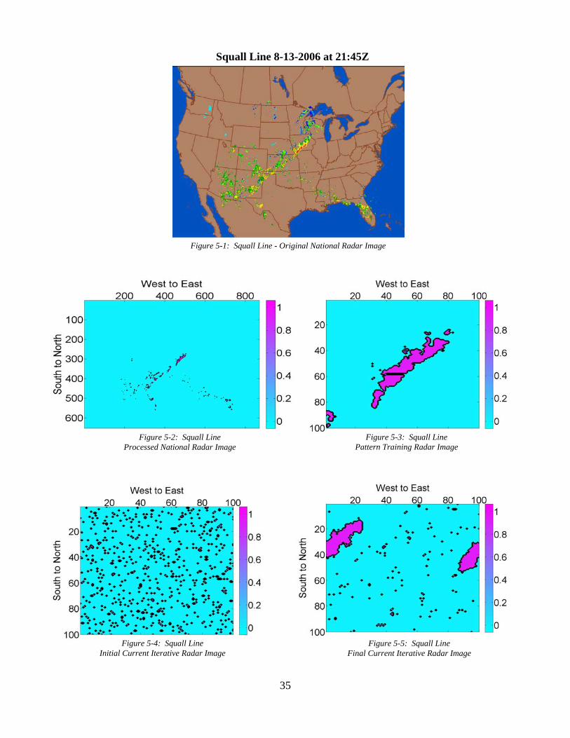
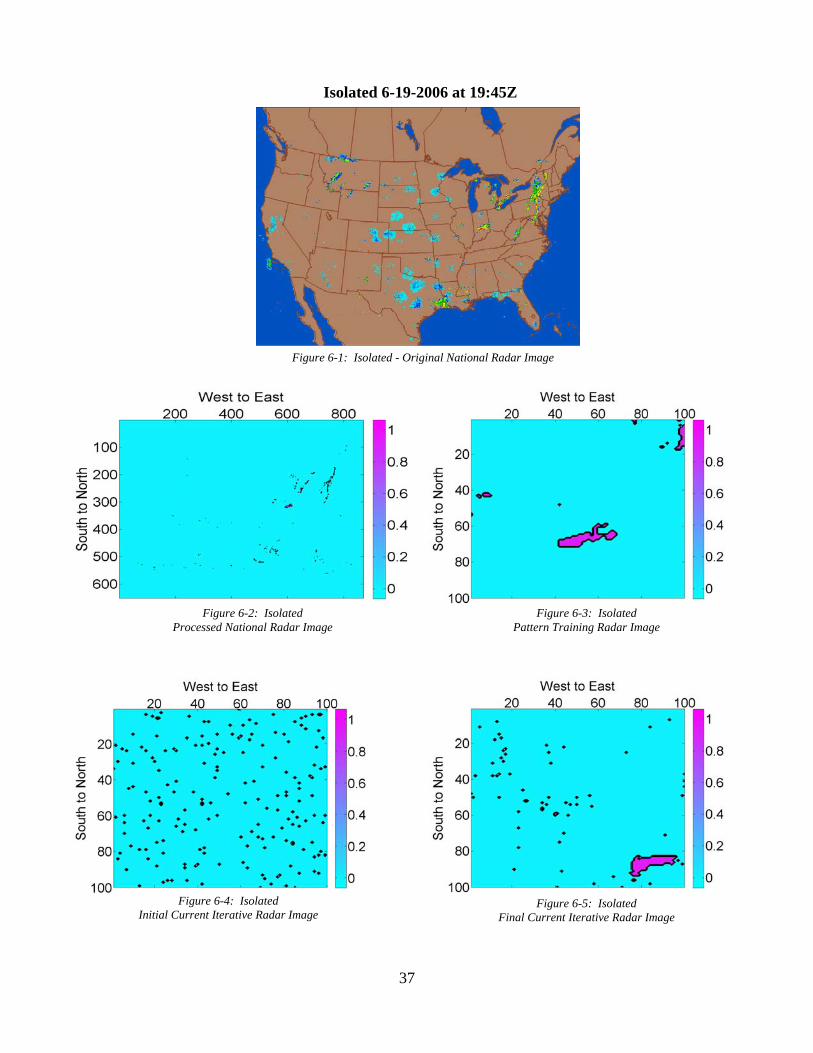
1. Original national radar image: An original 6 km national composite radar image from
NEXRAD radars, from which the case was identified for inclusion in algorithm processing.
2. Processed national radar image: A processed version of the original national radar image
depicting reflectivities 40 dBZ and greater as convective pixels with a value of one, non-
convective pixels with a value of zero. The color bar indicates pixel values while the x and y
axes indicate the number of pixels West to East and North to South.
3. Pattern training radar image: A 100 pixel by 100 pixel subsection of the processed national
radar image, containing the convective area of interest. Convective pixels have a value of
one and non-convective pixels have a value of zero. The color bar indicates pixel values
while the x and y axes indicate the number of pixels West to East and North to South.
4. Initial current iterative radar image: The initial version of the current iterative radar image
containing the correct convective coverage percentage as a fractional area of randomly
assigned convective pixels. Convective pixels have a value of one and non-convective pixels
have a value of zero. The color bar indicates pixel values while the x and y axes indicate the
number of pixels West to East and North to South.
5. Final current iterative radar image: The final processed version of the current iterative radar
image containing the correct convective coverage percentage and a pattern based off of the
pattern in the pattern training radar image. Convective pixels have a value of one and non-
convective pixels have a value of zero. The color bar indicates pixel values while the x and y
axes indicate the number of pixels West to East and North to South.
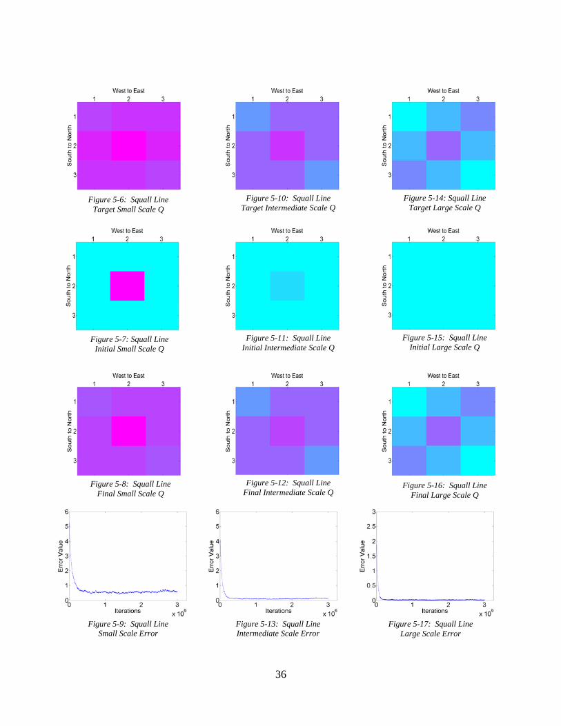
6. Target small scale Q: The small scale Q of the pattern training radar image. The shading
indicates the value of the conditional probability in the nine boxes of the Q matrix, where
magenta indicates a value of one (convective) and cyan indicates a value of zero
30
(nonconvective). The x and y axes indicate the box numbers of the Q matrix West to East
and North to South.
7. Initial small scale Q: The small scale Q of the initial version of the current iterative radar
image. The shading indicates the value of the conditional probability in the nine boxes of the
Q matrix, where magenta indicates a value of one (convective) and cyan indicates a value of
zero (nonconvective). The x and y axes indicate the box numbers of the Q matrix West to
East and North to South.
8. Final small scale Q: The small scale Q of the final version of the current iterative radar
image. The shading indicates the value of the conditional probability in the nine boxes of the
Q matrix, where magenta indicates a value of one (convective) and cyan indicates a value of
zero (nonconvective). The x and y axes indicate the box numbers of the Q matrix West to
East and North to South.
9. Small scale error: The small Q scale error value as a function of 3 million iterations where
the number of iterations is on the x axis and the value of the error is depicted on the y axis.
10. Target intermediate scale Q: The intermediate scale Q of the pattern training radar image.
The shading indicates the value of the conditional probability in the nine boxes of the Q
matrix, where magenta indicates a value of one (convective) and cyan indicates a value of
zero (nonconvective). The x and y axes indicate the box numbers of the Q matrix West to
East and North to South.
11. Initial intermediate scale Q: The intermediate scale Q of the initial version of the current
iterative radar image. The shading indicates the value of the conditional probability in the
nine boxes of the Q matrix, where magenta indicates a value of one (convective) and cyan
31
indicates a value of zero (nonconvective). The x and y axes indicate the box numbers of the
Q matrix West to East and North to South.
12. Final intermediate scale Q: The intermediate scale Q of the final version of the current
iterative radar image. The shading indicates the value of the conditional probability in the
nine boxes of the Q matrix, where magenta indicates a value of one (convective) and cyan
indicates a value of zero (nonconvective). The x and y axes indicate the box numbers of the
Q matrix West to East and North to South.
13. Intermediate scale error: The intermediate Q scale error value as a function of 3 million
iterations where the number of iterations is on the x axis and the value of the error is depicted
on the y axis.
14. Target large scale Q: The large scale Q of the pattern training radar image. The shading
indicates the value of the conditional probability in the nine boxes of the Q matrix, where
magenta indicates a value of one (convective) and cyan indicates a value of zero
(nonconvective). The x and y axes indicate the box numbers of the Q matrix West to East
and North to South.
15. Initial large scale Q: The large scale Q of the initial version of the current iterative radar
image. The shading indicates the value of the conditional probability in the nine boxes of the
Q matrix, where magenta indicates a value of one (convective) and cyan indicates a value of
zero (nonconvective). The x and y axes indicate the box numbers of the Q matrix West to
East and North to South.
16. Final large scale Q: The large scale Q of the final version of the current iterative radar
image. The shading indicates the value of the conditional probability in the nine boxes of the
Q matrix, where magenta indicates a value of one (convective) and cyan indicates a value of
32
zero (nonconvective). The x and y axes indicate the box numbers of the Q matrix West to
East and North to South.
17. Large scale error: The large Q scale error value as a function of 3 million iterations where the
number of iterations is on the x axis and the value of the error is depicted on the y axis.
Note: The images are organized according to case. Each image is assigned a figure number,
which consists of a case identification number followed by the image number from the
descriptive list above (i.e. case number-image number).
33
Figure 4-1: Front - Original National Radar Image
Figure 4-3: Front Pattern Training Radar Image
Figure 4-4: Front Initial Current Iterative Radar Image
Figure 4-5: Front Final Current Iterative Radar Image
Figure 4-2: Front Processed National Radar Image
Front Segment 9-23-2006 at 19:45Z
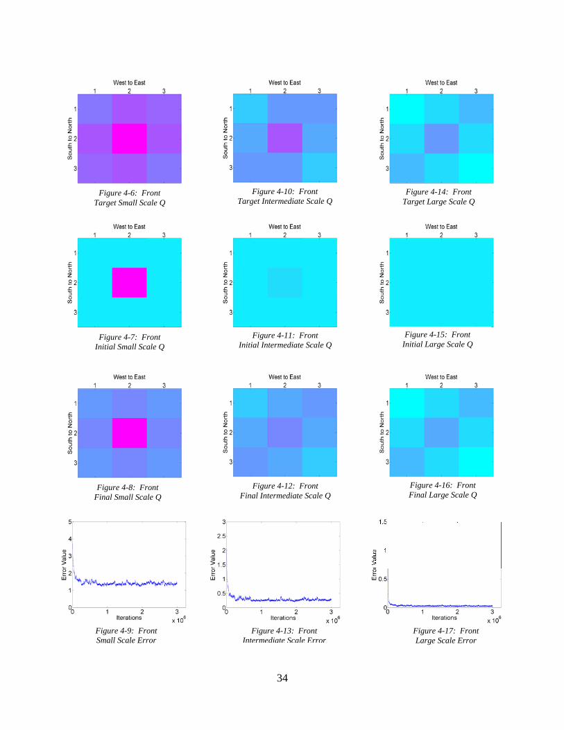
34
Figure 4-9: Front Small Scale Error
Figure 4-13: Front Intermediate Scale Error
Figure 4-17: Front Large Scale Error
Figure 4-6: Front Target Small Scale Q
Figure 4-10: Front Target Intermediate Scale Q
Figure 4-14: Front Target Large Scale Q
Figure 4-7: Front Initial Small Scale Q
Figure 4-11: Front Initial Intermediate Scale Q
Figure 4-15: Front Initial Large Scale Q
Figure 4-8: Front Final Small Scale Q
Figure 4-12: Front Final Intermediate Scale Q
Figure 4-16: Front Final Large Scale Q
35
Figure 5-1: Squall Line - Original National Radar Image
Figure 5-3: Squall Line Pattern Training Radar Image
Figure 5-4: Squall Line Initial Current Iterative Radar Image
Figure 5-5: Squall Line Final Current Iterative Radar Image
Figure 5-2: Squall Line Processed National Radar Image
Squall Line 8-13-2006 at 21:45Z
36
Figure 5-9: Squall Line Small Scale Error
Figure 5-13: Squall Line Intermediate Scale Error
Figure 5-17: Squall Line Large Scale Error
Figure 5-6: Squall Line Target Small Scale Q
Figure 5-10: Squall Line Target Intermediate Scale Q
Figure 5-14: Squall Line Target Large Scale Q
Figure 5-7: Squall Line Initial Small Scale Q
Figure 5-11: Squall Line Initial Intermediate Scale Q
Figure 5-15: Squall Line Initial Large Scale Q
Figure 5-8: Squall Line Final Small Scale Q
Figure 5-12: Squall Line Final Intermediate Scale Q
Figure 5-16: Squall Line Final Large Scale Q
37
Figure 6-1: Isolated - Original National Radar Image
Figure 6-3: Isolated Pattern Training Radar Image
Figure 6-4: Isolated Initial Current Iterative Radar Image
Figure 6-5: Isolated Final Current Iterative Radar Image
Figure 6-2: Isolated Processed National Radar Image
Isolated 6-19-2006 at 19:45Z

38
Figure 6-9: Isolated Small Scale Error
Figure 6-13: Isolated Intermediate Scale Error
Figure 6-17: Isolated Large Scale Error
Figure 6-6: Isolated Target Small Scale Q
Figure 6-10: Isolated Target Intermediate Scale Q
Figure 6-14: Isolated Target Large Scale Q
Figure 6-7: Isolated Initial Small Scale Q
Figure 6-11: Isolated Initial Intermediate Scale Q
Figure 6-15: Isolated Initial Large Scale Q
Figure 6-8: Isolated Final Small Scale Q
Figure 6-12: Isolated Final Intermediate Scale Q
Figure 6-16: Isolated Final Large Scale Q
39
Figure 7-1: Scattered - Original National Radar Image
Figure 7-3: Scattered Pattern Training Radar Image
Figure 7-4: Scattered Initial Current Iterative Radar Image
Figure 7-5: Scattered Final Current Iterative Radar Image
Figure 7-2: Scattered Processed National Radar Image
Scattered 8-7-2008 at 23:45Z
40
Figure 7-9: Scattered Small Scale Error
Figure 7-13: Scattered Intermediate Scale Error
Figure 7-17: Scattered Large Scale Error
Figure 7-6: Scattered Target Small Scale Q
Figure 7-10: Scattered Target Intermediate Scale Q
Figure 7-14: Scattered Target Large Scale Q
Figure 7-7: Scattered Initial Small Scale Q
Figure 7-11: Scattered Initial Intermediate Scale Q
Figure 7-15: Scattered Initial Large Scale Q
Figure 7-8: Scattered Final Small Scale Q
Figure 7-12: Scattered Final Intermediate Scale Q
Figure 7-16: Scattered Final Large Scale Q
41
Figure 8-1: Cluster - Original National Radar Image
Figure 8-3: Cluster Pattern Training Radar Image
Figure 8-4: Cluster Initial Current Iterative Radar Image
Figure 8-5: Cluster Final Current Iterative Radar Image
Figure 8-2: Cluster Processed National Radar Image
Cluster 8-23-2006 at 10:45Z
42
Figure 8-9: Cluster Small Scale Error
Figure 8-13: Cluster Intermediate Scale Error
Figure 8-17: Cluster Large Scale Error
Figure 8-6: Cluster Target Small Scale Q
Figure 8-10: Cluster Target Intermediate Scale Q
Figure 8-14: Cluster Target Large Scale Q
Figure 8-7: Cluster Initial Small Scale Q
Figure 8-11: Cluster Initial Intermediate Scale Q
Figure 8-15: Cluster Initial Large Scale Q
Figure 8-8: Cluster Final Small Scale Q
Figure 8-12: Cluster Final Intermediate Scale Q
Figure 8-16: Cluster Final Large Scale Q
43
Radar Image Generational Algorithm Strengths:
The radar image generational algorithm is capable of accurately reproducing the width of
the widest area of convection depicted on the pattern training radar image. This can be
seen in all of the example cases when the pattern training radar image is compared to the
final current iterative radar image (i.e. compare Figure 4-3 to Figure 4-5, Figure 5-3 to
Figure 5-5, Figure 6-3 to Figure 6-5, Figure 7-3 to Figure 7-5, and Figure 8-3 to Figure 8-
5). In every case, the greatest convective element width that appears on the current
iterative radar image is similar to the greatest convective element width that appears on
the pattern training radar image.
The general orientation or directionality of convection in the pattern training radar image
is well represented in the current iterative radar image. This is apparent in every example
case pairing of pattern training radar image and current iterative radar image.
The convective coverage percentage is accurately portrayed in the final version of the
current iterative radar image. This is apparent in Figures 4-5, 5-5, 6-5, 7-5, and 8-5.
The algorithm is particularly skilled at resolving unbroken linear convection as seen in
the pattern training radar image and depicting it in the final version of the current
iterative radar image. This is most obvious in linearly organized convective patterns such
as front segments and squall lines (i.e. compare Figure 4-3 to Figure 4-5 and Figure 5-3
to Figure 5-5).
The error value is effectively driven down by the algorithm in all cases and at all scales
(i.e. Figures 4-9, 4-13, 4-17; Figures 5-9, 5-13, 5-17; Figures 6-9, 6-13, 6-17; Figures 7-9,
7-13, 7-17; and Figures 8-9, 8-13, 8-17). The use of 3 million iterations allowed the
algorithm to be successful in achieving an error value which asymptotes as the number of
44
iterations increases. In all cases, the largest scale achieved the lowest final error value.
This is reflected in the image of the final large scale Q, a strength discussed in the next
bullet.
The final Q images are more similar to the corresponding target Q images than the initial
Q images at each scale for each case. This again reflects the success of the algorithm in
using the spatial conditional probability map (Q) to create a final current iterative radar
image reflecting the correct convective pattern. This is seen by individually comparing
the small scale Q panel (i.e. Figures 4-6, 4-7, 4-8; Figures 5-6, 5-7, 5-8; Figures 6-6, 6-7,
6-8; Figures 7-6, 7-7, 7-8; and Figures 8-6, 8-7, 8-8), intermediate scale Q panel (i.e.
Figures 4-10, 4-11, 4-12; Figures 5-10, 5-11, 5-12; Figures 6-10, 6-11, 6-12; Figures 7-
10, 7-11, 7-12; and Figures 8-10, 8-11, 8-12), and large scale Q panel (i.e. Figures 4-14,
4-15, 4-16; Figures 5-14, 5-15, 5-16; Figures 6-14, 6-15, 6-16; Figures 7-14, 7-15, 7-16;
and Figures 8-14, 8-15, 8-16) for each case. Note that in every case the large scale Q
panel has the most similar target and final Q images compared to the small and
intermediate Q scale panels. This directly ties back to the observation that the error value
at the large scale achieves the lowest value in all cases.
Radar Image Generational Algorithm Weaknesses:
Broken or separated areas of convection depicted in a pattern training radar image are not
resolved well by the algorithm in the current iterative radar image. This is most obvious
in the cases categorized as scattered convection and can be seen in the scattered
convection example (i.e. compare Figure 7-3 to Figure 7-5). However in the same
example case of scattered convection, it is apparent that the algorithm is “trying” to
resolve the broken convection, as evidence by the small clumps of convection that appear
45
in Figure 7-5. The error plots in Figures 7-9, 7-13, and 7-17 do confirm that the error is
minimized though. So an increase in the number of iterations would likely not result in
resolving the broken convection better.
The algorithm has difficulty tapering off the width in a narrowing area of convection
displayed in the pattern training radar image and resolving it in the current iterative radar
image. The best example of this is the front segment. When the pattern training radar
image in Figure 4-3 is compared to the final current iterative radar image in Figure 4-5, it
is obvious that the front segment in the current iterative radar image is shorter and retains
an invariant width equivalent to that of the widest area of convection in the pattern
training radar image.
The algorithm is not skilled at portraying patterns in pattern training radar images that are
characterized by convection of varying orientation or directionality. This is a weakness
largely relegated to the scattered convective pattern category. This weakness is relatively
less significant and is not portrayed in any of the example cases.
The algorithm is also not skilled at depicting the occasionally curved nature of linear
convection as portrayed in the pattern training radar image and resolving it in the current
iterative radar image. Linear convection may become curved in the form of a bow echo
or a large elongated front. The latter is not an issue on the smaller scale maps the
algorithm is processing here but the former has the potential to be an issue. This
weakness is relatively less significant and is not portrayed in any of the example cases.
Overall, using the spatial conditional probability maps are fairly effective as a means to
quantitatively compare the convective pattern on the pattern training radar image to the
46
convective pattern on the current iterative radar image. Most importantly, employing spatial
conditional probability maps in the radar image generational algorithm successfully produces a
radar image realization containing both the correct convective coverage percentage and, in
general, a pattern similar to that of the pattern training radar image, although weaknesses do
exist. Thus, the goal of the algorithm is achieved.
4.3 Statistical Analysis Results
In order to automate the selection of the pattern training spatial conditional probability
maps, a statistical analysis is performed to find atmospheric variables that correlate well with the
five convective pattern categories (i.e. front segment, squall line, isolated convection, scattered
convection, and clustered convection). The use of atmospheric variables to classify cases into
the five convective pattern categories achieves a poor percentage of correctly classified cases.
This leads to the use of a simpler statistical analysis, where atmospheric variables are used to
classify cases based on the two convective pattern types (i.e. linear convection and random
convection). This second method is much more successful but this remains an area in need of
future research.
As detailed in the procedures chapter, atmospheric variables included in the statistical
analysis include the K-index, Convective Available Potential Energy (CAPE), Convective
Inhibition (CIN), the presence or absence of a front in the vicinity, and wind shear from the
surface to 3000 m, 3000 m to 6000 m, and the surface to 6000 m. Matlab cluster analysis is
unsuccessful at grouping the cases into the five convective pattern categories using the available
atmospheric variables. The regression analysis in Weka is more successful and user friendly.
For these reasons, further statistical analysis is strictly done in Weka.
47
Various types of regression analyses are explored in Weka to find the atmospheric
variables that correctly classify the highest percentage of cases based on the five convective
categories. Another way to interpret this is that the analysis is using the atmospheric variables to
“forecast” the convective category associated with each case. The most successful statistical
analysis is one that has the most “forecasts” that agree with the actual convective category case
designations, as assigned in the manual analysis. Weka did poorly with few predictors, when
predictors were eliminated, indicating the predictors are valuable. In many instances though,
Weka is easily overfit with too many predictors when all predictors are included. When the
analyses are forced to forecast five convective categories, the resulting percentage of correctly
classified cases is very low. The percentage of correctly classified cases achieved is no more
than 35% in most instances.
Due to the poor results achieved using five convective categories, the second simpler
method of using only two convective pattern types is employed. This second method is much
more successful and achieves higher percentages of correctly classified cases. The best analysis,
achieving the highest percentage of correctly classified cases, is the logistic regression analysis,
which achieves a value of 68.9% correctly classified cases. This analysis is most successful
using all the variables except the presence of a front. So the logistic regression analysis is able to
accurately forecast the convective pattern type for a given case, based on the values of its
atmospheric variables, 68.9% of the time. While this value is much higher than the percentage
of correctly classified cases achieved using five convective categories, it is still not ideal for
automating the algorithm selection of the pattern training radar image. If this were implemented
as is, the algorithm would incorrectly select the appropriate pattern training radar image based on

48
the forecasted value of the atmospheric variables 31.1% of the time. Future work is planned to
attain higher percentages of correctly classified cases.
49
CHAPTER 5: CONCLUSIONS
The Federal Aviation Administration is responsible for managing the flow of air traffic
and maximizing air space capacity. The impediment weather poses to flight routes necessitates
convective forecasts. The radar image generational algorithm developed attempts to improve
upon the FAA forecasting standards in place by creating an ensemble of radar image realizations
that fit both the likely convective pattern and the forecasted convective probability. The
inclusion of convective forecasts throughout a space, as opposed to point forecasts would be
revolutionary in the FAA forecasting system. The creation of a radar image ensemble also
allows the FAA to factor in a measure of uncertainty of the impact that convective storms will
have on air space capacity and air traffic routes. Given the successful implementation of the
radar image generational algorithm into air traffic calculation and associated rules, there will be
considerable savings to the airlines and consumers.
The radar image generational algorithm is successful at combining a convective
probability with a convective pattern to achieve a single radar image realization. The algorithm
is capable of accurately depicting the convective coverage percentage, the general convective
pattern, the orientation of the convective pattern, and the width of the widest area of convection
through successfully minimizing the error value between the spatial conditional probability maps
of the pattern training radar image and the current iterative radar image. The most noteworthy
weakness of the algorithm is that it struggles to accurately resolve broken or separated areas of
convection. Algorithm output suggests that the algorithm is attempting to include the broken
areas of convection in its depiction of the forecasted radar image but it is not always successful.
50
The statistical analysis conducted to automate the selection of the pattern training radar
image in the algorithm, through finding the most highly correlated atmospheric variables and
using those variables to forecast the pattern training radar image, was fairly successful but will
remain an area for future work. The logistic regression analysis used atmospheric variables to
correctly classify 68.9% of cases based on the two convective pattern types. Yet this means that
when implemented the algorithm will incorrectly select a pattern training radar image in 31.1%
of cases. More analysis to maximize the percentage of correctly classified cases is required.
Once completed successfully, the algorithm will require only a forecasted convective probability
and a forecast of the appropriate atmospheric variables in order to derive the necessary spatial
conditional probability maps used to find the radar image forecast.
5.1 Future Work:
Several areas in need of future work remain. First, the statistical analysis to automate the
selection of the pattern training radar image must be concluded. Two paths remain an option.
The statistical analysis can be continued in an effort to maximize the percentage of correctly
classified cases using atmospheric variables as a classifying tool. This path involves
incorporating 3 hour RUC model sounding data instead of the 12 hour archived observed
sounding data, in an effort to obtain soundings that are not only at a more appropriate time near
that of the observed convective storm but are more aligned with the forecasting objective of the
algorithm.
The other available path to automate the selection of the pattern training radar image and
its associated spatial conditional probability maps is to develop an analog method as an
alternative to employing well correlated atmospheric variables to select the pattern training radar
51
image. An analog method would involve developing a database of various cases, associated
atmospheric variables, and associated spatial conditional probability maps. This database would
be used in conjunction with the inputted forecasted atmospheric variables to find the spatial
conditional probability maps for the pattern training radar image. Three database cases with
atmospheric variables values most similar to the forecasted atmospheric variables would be
selected. The three spatial conditional probability maps associated with the three database cases,
would be averaged to achieve the set of spatial conditional probability maps for the pattern
training radar image.
Another area in need of future work has to do with the assumption that the convective
probability, forecasted in LAMP, is equivalent to the fractional area of convective coverage, the
fraction of pixels assigned a convective designation in the initial current iterative radar image. In
reality a linear regression is needed to achieve the correct fractional area of convective coverage
from the convective probability presented in a grid in LAMP. This is planned to be implemented
in future versions of the radar image generational algorithm.
Lastly, the radar image generational algorithm has not addressed time progression in its
radar image forecasts. How a time series of radar image forecasts will be related is yet to be
determined. Ideally, the radar image forecasts would resemble and grow off of previous
forecasts. Currently though, successive use of the algorithm with new forecast variables, to
create a time series of ensemble radar image forecasts would yield completely separate, perhaps
unrelated, images. This will be an area requiring a lot of attention before the algorithm can be
successfully implemented in FAA air traffic forecasting rules.
52
REFERENCES
“About the Radar Operations Center.” NOAA’s National Weather Service Radar Operations Center. 9 Feb 2010. Web. Feb 2010. <http://www.roc.noaa.gov/WSR88D/About.aspx>. “The Collaborative Convective Forecast Product (CCFP)”. Collaborative Decision Making. Federal Aviation Administration. 15 Aug 2002. Web. Feb 2010. <http://cdm.fly.faa.gov/Workgroups/WxApps/CCFP%20Information%20Paper%20Aug%2002.doc>. E-wall: The Electronic Map Wall. The Pennsylvania State University Department of Meteorology. N.d. Web. 2006-2008. <http://www.meteo.psu.edu/ewall/ewall.html>.
HPC’s Surface Analysis Archive. Hydrometeorological Prediction Center. 1 Mar 2007. Web. Feb 2010. <http://www.hpc.ncep.noaa.gov/html/sfc_archive.shtml>.
Traffic Flow Management in the National Airspace System. Federal Aviation Administration Air Traffic Organization. Oct 2009. Web. Feb 2010. <http://www.fly.faa.gov/Products/Training/Traffic_Management_for_Pilots/TFM_in_the_NAS_Booklet_ca10.pdf>. Upper Air Sounding. University of Wyoming College of Engineering Department of Atmospheric Science. N.d. web. Feb 2010. <http://weather.uwyo.edu/upperair/sounding.html>. “What is a radiosonde?” National Weather Service Radiosonde Observations. National Weather Service. N.d. Web. Feb 2010. <http://www.ua.nws.noaa.gov/factsheet.htm>. What We Do. Federal Aviation Administration. 10 Mar 2010. Web. Feb 2010. <www.faa.gov/about/mission/activitiesl>. Wilks, Daniel S., 2006. Statistical Methods in the Atmospheric Sciences. 2nd ed. Amsterdam: Academic. 220 pp. Witten, I.H., and E. Frank, 2005. Data Mining, Practical Machine Learning Tools and Techniques, 2nd Edition. Morgan Kaufmann, San Francisco, CA, 525 pp.