CMS DN-11-000

2012/07/31

Improving the Identification of Electromagnetic Showers inthe CMS Forward Hadron Calorimeter at the LHC

C. Frye, K. Klapoetke, and J. MansUniversity of Minnesota, Minneapolis, United States of America

Abstract

The CMS Forward Hadron Calorimeter (HF) lies in a pseudorapidity region whichis not covered by the inner tracking system, and we can rely only on the shapes ofshowers that hit the detector to determine whether they are due to electromagneticparticles or jets. We review the current method of distinguishing these two types ofshowers in the HF, and we mention a drawback that will become present as the lu-minosity of the LHC increases and creates a need for tighter shower-shape cuts. Weprovide a method to correct this drawback, and we analyze the effectiveness of vari-ous tight cuts at isolating signal from background. We utilize data from proton-protoncollisions collected at CMS as well as Monte Carlo simulations to aid in the analysis.We also comment on the agreement of summer 2011 simulation, which utilized HFGFlash, and 2011 data.

1

1 IntroductionWe present improvements to current methods of distinguishing electromagnetic showers andjets in data collected using the Forward Hadron Calorimeter (HF) of the Compact Muon Solenoid(CMS) detector at the Large Hadron Collider. Current methods work well for the present LHCsetup, but as upgrades increase beam luminosity, an increased amount of pileup (i.e., unin-teresting secondary interactions) will require the use of tighter cuts to isolate electromagneticshowers from the background. These tighter cuts will expose flaws in our current methods,including a cut effectiveness that depends on shower energy. We correct this drawback andconsider techniques to maximize the effectiveness of tighter shower-shape cuts.

The ability to better reconstruct events in the HF will increase our accuracy in measurementssuch as Z → e+e− rapidity and forward-backward asymmetry, in detection of events such asW+ → e+ν, and in the search for H → ZZ(∗) → e+e−`+`−.

In [1], we presented our first results on electromagnetic identification in the HF using early2010 proton-proton collision data from CMS and Monte Carlo produced in spring, 2010. Herewe provide an update on those efforts, showing improvements made to the methods describedthere. We use 2011 data from proton-proton collisions that occurred at center-of-mass energiesof 7 TeV and Monte Carlo produced in the summer of 2011 in this analysis. This is the first setof Monte Carlo produced with the HF GFlash upgrade, and we compare this simulation to thedata to evaluate its integrity.

We begin by briefly describing the design of the HF and move on to give more detail aboutthe samples on which we performed the analysis presented here. We then give an overview ofthe HF event reconstruction process developed in [1]. Next, we explain the methods by whichwe currently identify electromagnetic showers in the HF, and we present our main results con-cerning improvements to these methods.

2 The Forward Hadron CalorimeterThe rate of particle production as a function of pseudorapidity in CMS is roughly constant.However, the surface area of the detector per unit pseudorapidity, |dA/dη|, decreases consid-erably at high values of |η|. Also, average energy per particle increases as |η| becomes large.The HF, located in the region 3 < |η| < 5, thus experiences showers with high energy densityduring collisions. Because of the high dose of radiation it receives, the HF was built from moreradiation-resistant materials than other parts of the hadronic calorimeter in CMS.

The HF consists of steel absorber plates containing quartz fibers which run parallel to the beam-line and relies on Cerenkov light produced in these fibers to detect showers. (See Figure 1 forthe layout of the Forward Hadron Calorimeter.) The quartz fibers are of two different lengths.Long fibers extend 1.65 meters from the rear of the HF to its inner face, while short fibers extend1.43 meters from the rear and leave a 0.22 meter gap filled with steel between their ends andthe inner face of the detector.

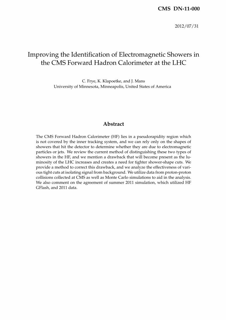
Each of the two HF calorimeters (one for positive η, one for negative η) is divided into 18wedges, each containing 24 towers (see Figure 2). Each tower (also referred to as a cell be-low) is a “square” of side 0.171 in ηφ-space, except the towers in the innermost and outermostrings of the detector, as can be seen in the figure. The outermost cells have a shorter η dimen-sion because, being in the shadow of the end-cap calorimeters, they serve only to measure thetransverse shower leakage from the rest of the HF.

2 3 Data and Monte Carlo Samples

Absorber

Concrete Shielding

Steel Shielding

Polyethylene Shielding

Steel Plug Shielding

Light GuidesReadout Boxes

Poly

eth

lene S

hie

ldin

g

Figure 1: Cross-sectional view of the HF, where r increases vertically and z increases to theleft (i.e., showers enter from the right). Steel absorber plates and other shielding is shown.Photomultipliers are located in the readout boxes. The vertical dashed red line marks the endof the short fibers.

Each HF tower connects to two photomultiplier tubes (PMTs). One PMT reads the energyabsorbed by the long fibers of that tower while the other PMT is associated with the shortfibers. In Section 4 we provide a discussion of hit reconstruction beginning at the stage of thePMTs. For documentation of the performance of the HF detector in test beam runs, see [2].

3 Data and Monte Carlo SamplesWe use 1.01 fb−1 of DoubleElectron data from Run2011A, specifically,

• Run2011A/DoubleElectron/RECO/05Jul2011ReReco-HF.

In our analysis, we predominantly use events that passed the high-level trigger,

• HLT Ele17 CaloIdL CaloIsoVL Ele15 HFL,

(referred to as the HLT below), which requires a loose 17 GeV electron to be received in theElectron Calorimeter (ECAL) and a loose1 15 GeV electron to be received in the HF.

To obtain signal from this data, we apply a skim, which requires the ECAL electron to passWP80 requirements (see [3]) and the event to have an invariant mass in the Z window, 70-120GeV/c2. We subsequently require the signal to pass a selection which applies a series of loosecuts (similar to those in the skim) on the shower-shape variables of the HF electron introducedin Subsection 5.1 as well as further cuts on the ECAL electron. We will refer to this sample as

1A “loose” electron here is one that passed the lateral containment cut E9/25 ≥ 0.92, see equation (2), and the 2dcut in equation (3) with C2d = 0.2.

3

414039

3837

3635

34

33

32

31

30

29

5.21

4.90

4.74

4.55

4.38

4.20

4.03

3.85

3.68

3.50

3.33

3.15

2.98

2.87

67

69

71

1

3

5

Figure 2: Three adjacent wedges of HF, each spanning ∆φ = 20◦, shown in rφ-space. Indices onthe upper and outer edges are called iη and iφ, respectively. The values along the lower edgedenote the η-values of the cell boundaries. As introduced in Section 4.3, the shading depictsthe seed cell (in yellow), 3× 3 region (green + yellow), and 5× 5 region (blue + green + yellow)of an electromagnetic cluster.

“Data: Signal” below in the figures.

We get background from this data by taking all events that fail the selection mentioned above.We also apply a cut on the invariant mass of background events, requiring 70 GeV/c2 < m <120 GeV/c2. We refer to this sample as “Data: Background” below. By imposing these re-quirements, we use background similar to the pileup that will be difficult to reject as the LHCluminosity increases.

We also use simulated signal Monte Carlo from Summer11, specifically,

• Summer11/DYToEE M-20 TuneZ2 7TeV-pythia6/GEN-SIM-RECO/PU S3 START42 V11-v2.

This is the first set of CMS Monte Carlo that was produced using HF GFlash, which createssimulation up to ten thousand times faster than Geant4 which was previously used. We requirethis to pass the same selection imposed on “Data: Signal,” and in the figures we call this sample“Monte Carlo: Signal.”

In one of the studies below, we compare the performance of summer Monte Carlo to that pro-duced in the spring. We use

• Spring11/DYToEE M-20 CT10 TuneZ2 7TeV-powheg-pythia/GEN-SIM-RECO/PU S1 START311 V1G1-v1.

4 4 Reconstruction Algorithms for HF Hits

We subject the spring simulation to the same selections imposed on summer simulation, andwe will refer to this sample below as “Spring MC: Signal.”

4 Reconstruction Algorithms for HF HitsWe have made no change to the reconstruction algorithms since the release of [1], and ourmethods are described there in detail. We give a summary of that information here for com-pleteness.

4.1 Local Reconstruction

Photomultiplier tubes are used to convert the Cerenkov light produced in the quartz fibersof the HF into electric charge, which is subsequently integrated and digitized by the ChargeIntegrator Encoder Application-specific Integrated Circuit (QIE ASIC). Separate pedestal runsallow for correction of the pedestal offset. Then the following gain factors are applied to thereceived charge: a base gain determined using test-beam data and a response correction deter-mined using measurements of φ-symmetry from collision data. Early collision data was alsoused to align the integration timing of the HF.

4.2 PMT Hit Rejection

One type of HF background is created when particles (usually muons) pass through HF anddirectly into a photomultiplier tube, generating Cerenkov light and causing a fake signal. TheHCAL DPG has developed several variables that can be used to remove PMT hits as well asother types of anomalous background. These techniques are documented in [4], and we usethe “Version 6 Cleaning” algorithm described there in our reconstruction. This algorithm wasdeveloped to provide strong anomalous hit rejection while still retaining signals from isolatedphotons.

When a PMT hit occurs in the same location as a jet, however, the combination could passelectron identification cuts; this type of PMT hit will not be removed by the above algorithm.This usually occurs in low-η regions of the detector and would likely be eliminated in standardbackground removal for any further physics search.

4.3 Clustering the Remaining Hits

So that noise from the electronics does not contribute to the data, we only accept hits withE > 4 GeV in the long fibers, which corresponds roughly to ET > 400 MeV (long fibers) at|η| = 3.

With the HF hits that pass this energy requirement and survive the PMT hit rejection describedabove, we form clusters as follows. We declare HF hits with ET > 5 GeV to be seed candidates.We consider all hits meeting this criterion in order of decreasing ET, removing as candidatesthose cells that lie within the 5× 5 tower matrix surrounding a seed candidate with higher ET.In this way, we avoid overlapping clusters.

For each of the surviving clusters, we define the raw cluster energy to be

Eraw = ∑i∈3×3

Li,

where Li is the energy absorbed by the long fibers in the i-th tower of the cluster matrix. We usethe 3× 3 matrix here because of its complete containment of electromagnetic showers. Even

4.4 Position Corrections 5

though the transverse size of electromagnetic showers is actually even smaller than one tower,we cannot use 1× 1 or 1× 2 matrices to measure total shower energy because of hits near aseed cell edge or corner. We define the core of a cluster to be the seed cell along with its highest-energy-absorbing neighbor, where this neighbor must absorb at least half as much energy asthe seed cell. If no such neighbor exists, the cluster core reduces to the seed cell alone.

The (η, φ)-position of a hit is calculated as the mean of the (η, φ)-coordinates of the towercenters in the cluster, each weighted by the natural logarithm of the tower’s absorbed energy;specifically,

ηraw =∑i∈3×3

[log(Li / 1 GeV)

]ηi

∑i∈3×3 log(Li / 1 GeV),

φraw =∑i∈3×3

[log(Li / 1 GeV)

]φi

∑i∈3×3 log(Li / 1 GeV),

where (ηi, φi) are the coordinates of the center of the i-th tower in the cluster. We weight thecells in this way because the logarithm of the energy absorbed in a hit is proportional to thepenetration depth of the corresponding hit.

4.4 Position Corrections

The coordinates (ηi, φi) in the previous section give the location of the inner face of the i-thtower in a cluster. Since the HF towers are parallel to the beam-line, we will be slightly off indetermining the position of a hit when the particle enters the tower some distance behind itsinner face. Because of this, η tends to be underestimated. Although this effect is dependent onshower depth and thus varies with energy, we use a constant additive correction Cbias which issufficient to remove this η-bias over the energy range typical in the HF.

A second type of position bias occurs as a result of our inability to determine the location ofa hit within a tower. Since, as mentioned before, the transverse size of a tower exceeds thatof an electromagnetic shower, systematic error develops when we calculate ηraw and φraw. Instudying this bias, we introduce variables to quantify relative location inside a cell,

ηcell =ηraw − |η|min

|η|max − |η|min,

φcell =φraw − φmin

φmax − φmin,

where |η|min, φmin (respectively |η|max, φmax) are the smallest (respectively largest) |η|, φ valuesfound in the seed cell of a cluster. In [1] we showed that the difference between Monte Carlotruth and ηraw (respectively φraw) depends sinusoidally on ηcell (respectively φcell).

Comparing data to Monte Carlo truth, we use the following position corrections (see [1] forfurther analysis of their impact). For reconstructed η we use

ηreco = ηraw + sgn(ηraw) · [Aη sin(2πηcell) + Cbias],Aη = 0.00683± 0.00013,

Cbias = 0.00938± 0.00009,

and for reconstructed φ we use

φreco = φraw + Aφ sin(2πφcell),Aφ = 0.00644± 0.00010.

6 5 Identification of Electromagnetic Showers

9/25E0.92 0.93 0.94 0.95 0.96 0.97 0.98 0.99 1 1.01

Arb

itra

ry U

nit

s

0

0.2

0.4

0.6

0.8

1

1.2

1.4Data: Signal

Data: Background

Monte Carlo: Signal

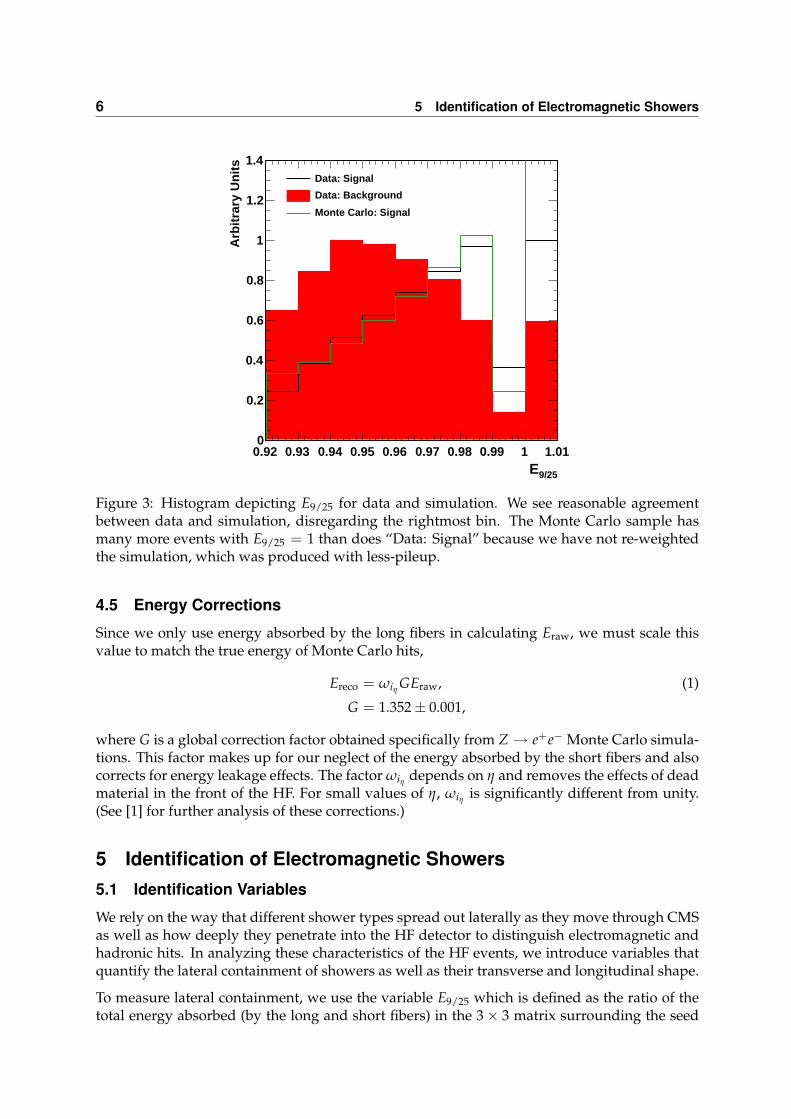
Figure 3: Histogram depicting E9/25 for data and simulation. We see reasonable agreementbetween data and simulation, disregarding the rightmost bin. The Monte Carlo sample hasmany more events with E9/25 = 1 than does “Data: Signal” because we have not re-weightedthe simulation, which was produced with less-pileup.

4.5 Energy Corrections

Since we only use energy absorbed by the long fibers in calculating Eraw, we must scale thisvalue to match the true energy of Monte Carlo hits,

Ereco = ωiηGEraw, (1)

G = 1.352± 0.001,

where G is a global correction factor obtained specifically from Z → e+e− Monte Carlo simula-tions. This factor makes up for our neglect of the energy absorbed by the short fibers and alsocorrects for energy leakage effects. The factor ωiη

depends on η and removes the effects of deadmaterial in the front of the HF. For small values of η, ωiη

is significantly different from unity.(See [1] for further analysis of these corrections.)

5 Identification of Electromagnetic Showers5.1 Identification Variables

We rely on the way that different shower types spread out laterally as they move through CMSas well as how deeply they penetrate into the HF detector to distinguish electromagnetic andhadronic hits. In analyzing these characteristics of the HF events, we introduce variables thatquantify the lateral containment of showers as well as their transverse and longitudinal shape.

To measure lateral containment, we use the variable E9/25 which is defined as the ratio of thetotal energy absorbed (by the long and short fibers) in the 3× 3 matrix surrounding the seed

5.1 Identification Variables 7

C/9E0.4 0.5 0.6 0.7 0.8 0.9 1

Arb

itra

ry U

nit

s

0

0.2

0.4

0.6

0.8

1

1.2

1.4Data: Signal

Data: Background

Monte Carlo: Signal

Figure 4: Histogram depicting EC/9 for data and simulation. Signal and background differa good deal even after both were required to pass the HLT. Real signal and simulated signalmatch quite well.

cell to that absorbed in the 5× 5 matrix, i.e.,

E9/25 = ∑i∈3×3(Li + Si)∑i∈5×5(Li + Si)

. (2)

Electromagnetic showers, which are composed of lighter particles than the hadrons in jets, re-main laterally dense as they propagate through CMS while jets tend to spread out. Because ofthis, electromagnetic showers are virtually completely contained in the 3× 3 matrix surround-ing the seed cell and have an E9/25 value of nearly unity; conversely, the value of E9/25 for jets isappreciably lower. In current methods of signal isolation [1], we use a cut E9/25 > 0.94, whichhas very high signal efficiency, to begin separating signal from background.

To quantify transverse shape, we use EC/9 which is defined as the ratio of the energy absorbedby the long fibers in the core matrix to that absorbed by the long fibers in the 3× 3 matrix ofthe cluster, i.e.,

EC/9 = ∑i∈core Li

∑i∈3×3 Li.

For the same reasons mentioned above, the value of EC/9 tends towards unity for electromag-netic showers and is significantly lower for jets (see Figure 4).

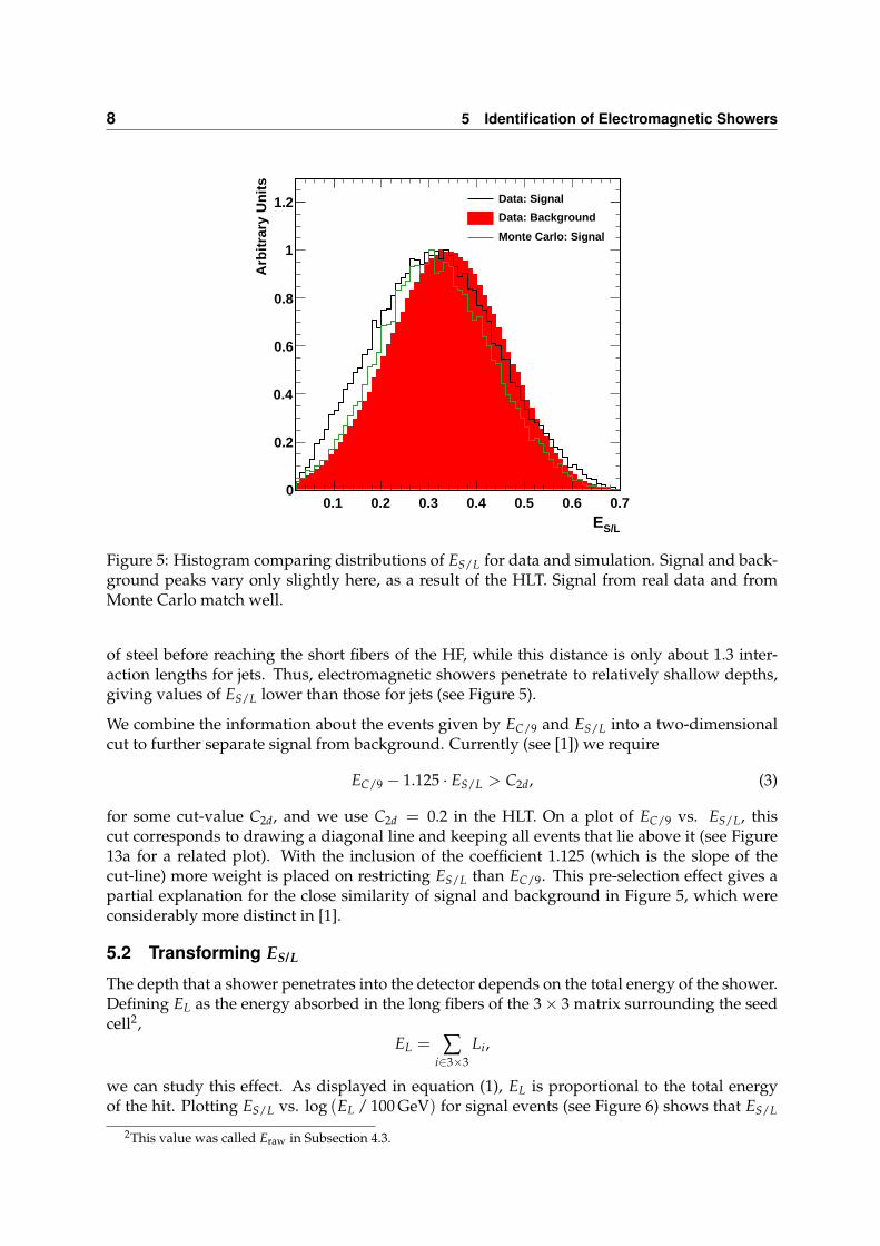
Finally, we measure the longitudinal shower shape with ES/L, defined as the ratio of the en-ergy absorbed by the short fibers in the 3 × 3 matrix of the cluster to that absorbed by thecorresponding long fibers, i.e.,

ES/L = ∑i∈3×3 Si

∑i∈3×3 Li,

where Si is the energy absorbed by the short fibers in the i-th cell of the cluster. As men-tioned in the introduction, electromagnetic showers must travel through 12.5 radiation lengths

8 5 Identification of Electromagnetic Showers

S/LE0.1 0.2 0.3 0.4 0.5 0.6 0.7

Arb

itra

ry U

nit

s

0

0.2

0.4

0.6

0.8

1

1.2 Data: Signal

Data: Background

Monte Carlo: Signal

Figure 5: Histogram comparing distributions of ES/L for data and simulation. Signal and back-ground peaks vary only slightly here, as a result of the HLT. Signal from real data and fromMonte Carlo match well.

of steel before reaching the short fibers of the HF, while this distance is only about 1.3 inter-action lengths for jets. Thus, electromagnetic showers penetrate to relatively shallow depths,giving values of ES/L lower than those for jets (see Figure 5).

We combine the information about the events given by EC/9 and ES/L into a two-dimensionalcut to further separate signal from background. Currently (see [1]) we require

EC/9 − 1.125 · ES/L > C2d, (3)

for some cut-value C2d, and we use C2d = 0.2 in the HLT. On a plot of EC/9 vs. ES/L, thiscut corresponds to drawing a diagonal line and keeping all events that lie above it (see Figure13a for a related plot). With the inclusion of the coefficient 1.125 (which is the slope of thecut-line) more weight is placed on restricting ES/L than EC/9. This pre-selection effect gives apartial explanation for the close similarity of signal and background in Figure 5, which wereconsiderably more distinct in [1].

5.2 Transforming ES/L

The depth that a shower penetrates into the detector depends on the total energy of the shower.Defining EL as the energy absorbed in the long fibers of the 3× 3 matrix surrounding the seedcell2,

EL = ∑i∈3×3

Li,

we can study this effect. As displayed in equation (1), EL is proportional to the total energyof the hit. Plotting ES/L vs. log (EL / 100 GeV) for signal events (see Figure 6) shows that ES/L

2This value was called Eraw in Subsection 4.3.

5.2 Transforming ES/L 9

)eVG001/LE(log0 0.5 1 1.5 2 2.5 3

S/L

E

0

0.1

0.2

0.3

0.4

0.5

0.6

0.7

0.8 Data: Signal

(a)

)eVG001/LE(log0 0.5 1 1.5 2 2.5 3

S/L

E

0

0.1

0.2

0.3

0.4

0.5

0.6

0.7

0.8 Monte Carlo: Signal

(b)

Figure 6: Plot showing ES/L vs. log (EL / 100 GeV) for (a) real signal and (b) simulated signal.The fit lines were obtained using the method described in the text.

increases with total shower energy for electromagnetic hits. Thus, if we use ES/L to make acut on a sample, we may remove high-energy electromagnetic events because their penetrationdepth (measured by ES/L) disguised them as jets.

To remove the dependence of ES/L on EL for signal, we make a transformation that produces anew variable, E cor

S/L, which we call “Transformed ES/L” in the figures. An algorithm performsthe transformation using the ES/L vs. log (EL / 100 GeV) plot as follows. (In the paragraphsbelow, we refer to the horizontal axis of this plot as the x-axis and the vertical axis as the y-axisfor simplicity.)

First, we fit the points in the plot to a line. To do this we let xi step bin-by-bin along thehorizontal axis of the histogram, in each step considering all events having x = xi (these makeup a vertical strip). We fit the frequency of the events in this strip to a Gaussian function ofy which has mean yi, and we collect these points (xi, yi) for each step in the process. We thenfit the points (xi, yi) to a line, taking into account the errors, thus obtaining two constants m, bwhich are the slope and y-intercept of the line, respectively. To neglect outliers, we consideronly those vertical strips that contain at least 1% of the total entries in the histogram. Second,we choose an arbitrary point x0 on the horizontal axis, and we translate all points in the plotso that (x0, mx0 + b) becomes the origin. Third, we rotate the entries in the plot clockwise byangle tan−1(m) after which the fit line coincides with the x-axis. We then call the new y-valueof each point E cor

S/L.

This transformation sends each point (x, y) in the plot to the new point (x, y′), and the trans-

10 5 Identification of Electromagnetic Showers

)eVG001/LE(log0 0.5 1 1.5 2 2.5 3

S/L

Tran

sfo

rmed

E

-0.6

-0.4

-0.2

0

0.2

0.4

0.6

Data: Signal

(a)

)eVG001/LE(log0 0.5 1 1.5 2 2.5 3

S/L

Tran

sfo

rmed

E

-0.6

-0.4

-0.2

0

0.2

0.4

0.6

Monte Carlo: Signal

(b)

Figure 7: Plot showing E corS/L vs. log (EL / 100 GeV) for (a) real signal and (b) simulated signal.

After the transformation the distributions are flat, and a line fit to the dense regions of eventswould coincide with the x-axis.

formation can be written y 7→ y′ = α + βx + γy, where

α =−b√

1 + m2,

β =−m√1 + m2

,

γ =1√

1 + m2,

and b, m are the parameters of the fit line mentioned above. This is equivalent to sending(x, y) 7→ (x, y′) where y′ is the perpendicular distance from the point (x, y) to the line y =mx + b.

The fit lines are shown in Figure 6, and we compare all the constants involved in this trans-formation in the tables shown in Figure 8. We attribute the differences in the values of b, α fordata and simulation to the slight difference in the mean log (EL / 100 GeV)-value for the twosamples (shown as 〈x〉 in the table), which has the same order of magnitude. (The error in〈x〉 originates from the finite bin width in the histogram.) Also, in the tables we include thetransformation constants for “Spring MC: Signal,” in order to show the improvement madeby summer Monte Carlo in simulating the data. When we plot E cor

S/L vs. log (EL / 100 GeV) forsignal (see Figure 7), we see that the entries are “flat,” i.e., that the dependence of the longitudi-nal variable on the total energy of the corresponding shower is removed. We transform “Data:Background” with the same constants obtained for “Data: Signal.” We expect the backgroundevents to be located farther from the fit line than the signal events; hence, values of E cor

S/L shouldbe greater for background than for signal, which will allow us to make a useful cut with thisvariable.

5.3 Improving the Cuts 11

b m 〈x〉Data: Signal 0.008 ± 0.0042 0.221 ± 0.0030 1.34 ± 0.00084

Monte Carlo: Signal 0.037 ± 0.0032 0.200 ± 0.0022 1.37 ± 0.00084Spring MC: Signal -0.062 ± 0.0064 0.242 ± 0.0043 1.41 ± 0.00085

α β γ

Data: Signal -0.008 ± 0.0041 -0.216 ± 0.0028 0.9764 ± 0.00061Monte Carlo: Signal -0.036 ± 0.0031 -0.196 ± 0.0021 0.9806 ± 0.00042Spring MC: Signal 0.061 ± 0.0063 -0.235 ± 0.0039 0.9719 ± 0.00095

Figure 8: Parameters used for data and simulation in the transformation ES/L 7→ E corS/L. We

show values for spring Monte Carlo to compare how well spring and summer simulationmatch the data. Summer Monte Carlo simulates data more accurately than does spring MonteCarlo, as we see from the values of b, α, 〈x〉.

Signal Efficiency0.5 0.6 0.7 0.8 0.9 1

Bac

kgro

und

Rej

ectio

n

0

0.1

0.2

0.3

0.4

0.5

0.6

0.7 Cut on Data

S/LTransformed E

Cut on DataS/LE

Figure 9: Comparison of the ES/L and E corS/L cuts. For each value of signal efficiency, the E cor

S/Lgives greater background rejection.

5.3 Improving the Cuts

We performed a simple analysis to compare the effectiveness of the transverse, longitudinal,and two-dimensional shower shape cuts available to us using the variables EC/9, ES/L, E cor

S/L.Since our signal and background have already been required to pass the cuts described in Sec-tion 3, the goal of this analysis is to determine where small improvements can be made. Sinceour goal is to determine the optimal set of cuts to perform to isolate signal from background,we will focus mostly on the relative effects of the different cuts and less on there absolute effec-tiveness.

12 5 Identification of Electromagnetic Showers

Signal Efficiency0.5 0.6 0.7 0.8 0.9 1

Bac

kgro

und

Rej

ectio

n

0

0.1

0.2

0.3

0.4

0.5

0.6

0.7

0.8

0.9

1 Cut on DataC/9E

Current 2d Cut on Data

Figure 10: Comparison of the transverse and current two-dimensional cuts. For the tight cutsshown here, EC/9 is more effective than the cut in equation (3).

5.3.1 The Longitudinal Cut

First, we evaluate the improvement made by transforming the longitudinal shower shape vari-able. We consider a cut on the data requiring ES/L < C` and alternatively a cut requiringE cor

S/L < C′`, for some cut-values C`, C′`. In analyzing these cuts we consider

signal efficiency =# of signal events that survive cut

total # of signal events

andbackground rejection =

# of background events that fail cuttotal # of background events

.

We employ an algorithm that, using our data set, computes the background rejection as a func-tion of signal efficiency for each of the longitudinal cuts. We compare the ES/L and E cor

S/L cutsby plotting this information in Figure 9. We see in the figure that the E cor

S/L cut performs betterthan the ES/L cut for any desired signal efficiency. Thus, the ES/L cut should be replaced withthe Transformed ES/L cut in all cases.

5.3.2 The Transverse Cut

It is already known that the EC/9 cut is quite effective [1]. In fact, for tight selections, the EC/9cut is more effective than the two-dimensional cut in equation (3), which is currently in use.Indeed, we find in Figure 10 that for any given signal efficiency, the transverse cut rejects morebackground than the current 2d cut.

We now evaluate the benefits of combining this transverse shower shape cut with the longitu-dinal cut E cor

S/L. One way to combine these cuts is to perform them independently in succession,i.e., to require EC/9 > Ct and E cor

S/L < C` for some values of Ct, C`. On a plot of EC/9 vs. E corS/L,

5.3 Improving the Cuts 13

S/LTransformed E-0.4 -0.2 0 0.2 0.4 0.6

C/9

E

0.4

0.5

0.6

0.7

0.8

0.9

1

Data: Signal

(a)

Signal Efficiency0.5 0.6 0.7 0.8 0.9 1

Bac

kgro

und

Rej

ectio

n0

0.1

0.2

0.3

0.4

0.5

0.6

0.7

0.8

0.9

1 Cut on DataC/9E

Square Cut on Data

(b)

Figure 11: (a) EC/9 vs. E corS/L with example square cut-lines for “Data: Signal.” (b) Comparison

of the square cut and the EC/9 cut on data, which turn out to have nearly identical effects.

this corresponds to drawing a vertical line and a horizontal line and keeping only those eventsin the top-left corner of the plot (see Figure 11a). Hence, we call this the square cut. In using thiscut to obtain a certain signal efficiency, there are many combinations of Ct, C` that will work.We use a simple algorithm to perform the square cut with those values of Ct, C` that give thedesired signal efficiency and maximize the background rejection.

In Figure 11b, we compare the square cut to the EC/9 cut by plotting background rejectionversus signal efficiency for each of these cuts when performed on the data. We see that the twographs almost coincide, suggesting that in choosing the optimal values of Ct and C` the squarecut becomes the EC/9 cut. In Figure 11a, this corresponds to the vertical line being pushed allthe way to the right, making the square cut effectively a one-dimensional cut on EC/9. Thus,it is not effective to use the transverse and longitudinal cuts independently, and to simplifycoding we should always use the simpler EC/9 cut instead of the square cut.

5.3.3 The Two-dimensional Cut

Though EC/9 is quite effective on its own, we would like to gain some benefit from our knowl-edge of E cor

S/L. Hence, we introduce an optimized two-dimensional cut in the style of equation(3), where the transverse and longitudinal cuts are not performed independently. We require

EC/9 −m · E corS/L > C2d

for some values of m, C2d. Whereas the square cut corresponded to drawing two perpendicularlines on the plot in Figure 11a and requiring events to be located in the top-left corner, thistwo-dimensional cut draws one slanted line on the plot (see Figure 13a) with slope m and y-intercept C2d and requires events to be above this line. As in the square cut, we use an algorithmthat chooses values of m and C2d which give the desired signal efficiency while optimizingbackground rejection.

In Figure 13b, we graph background rejection versus signal efficiency to compare this new two-dimensional cut to the EC/9 cut. The new two-dimensional cut dominates over the transverse

14 6 Future Work

Efficiency 50% 55% 60% 65% 70% 75% 80% 85% 90% 95%C2d 0.90 0.88 0.87 0.85 0.83 0.81 0.78 0.74 0.71 0.64m 0.26 0.30 0.33 0.43 0.35 0.48 0.50 0.65 0.60 0.80

Figure 12: Optimized C2d, m values used in the new two-dimensional cut on data. Step size inthe optimization algorithm determines the error on these parameters: ∆C2d = 0.01, ∆m = 0.025.

S/LTransformed E-0.4 -0.2 0 0.2 0.4 0.6

C/9

E

0.4

0.5

0.6

0.7

0.8

0.9

1

Data: Signal

(a)

Signal Efficiency0.5 0.6 0.7 0.8 0.9 1

Bac

kgro

und

Rej

ectio

n

0

0.1

0.2

0.3

0.4

0.5

0.6

0.7

0.8

0.9

1 Cut on DataC/9E

Optimized 2d Cut on Data

(b)

Figure 13: (a) EC/9 vs. E corS/L with an example 2d cut-line for “Data: Signal.” (b) Comparison

of the new 2d cut and the EC/9 cut on data, where it is clear that the new 2d cut offers animprovement in background rejection.

cut alone for all signal efficiencies considered. Thus, it will create improvement in signal isola-tion to use the new two-dimensional cut as the cut of choice in distinguishing electromagneticshowers from jets. The optimized parameters C2d, m used in the new two-dimensional cut ondata are shown in Figure 12 for each value of signal efficiency.

6 Future WorkWe can further investigate the bias of the shower-shape cuts by studying the dependency ofthe signal efficiency of the EC/9 cut on total shower energy. Such a study will tell us whether ornot we need to perform a transformation of the transverse shower-shape variable to enhanceeffectiveness in tighter cuts.

We have begun this investigation using the “Data: Signal” sample. We produced two plotsof transverse momentum of the HF electron versus the invariant mass of the double-electronevent, one using the entire sample and the other using only those events that passed a cutEC/9 ≥ 0.845. This transverse shower-shape cut keeps roughly 70% of “Data: Signal” events.Since we are interested in pure signal efficiency, we attempted to disregard the background stillpresent in our sample as follows.

In our pT vs. mZ plots, we considered intervals ∆pT of transverse momentum and fit the events

15

(GeV) of HF electronT

p20 30 40 50 60 70 80 90 100

Sig

nal E

ffici

ency

0.65

0.7

0.75

0.8

0.85

Cut on 'Data:Signal'C/9E

Figure 14: Plot of modified signal efficiency versus transverse momentum of the HF electron.The efficiency depends of pT, showing that an improvement can be made in the transverseshower-shape variable.

in each range to a function f (mZ) of invariant mass. We required f (mZ) to be a Gaussiansuperimposed on a decaying exponential, where the Gaussian (with its peak in the Z-massrange and its width required to be the width of the Z-mass curve) corresponds to signal andthe decaying exponential corresponds to background. We then integrated the Gaussian part off (mZ) to determine the number of signal events that fall in the interval ∆pT. (In this processwe varied the size of ∆pT in order to accept enough events to obtain statistically significantresults.)

Performing this algorithm produced two histograms displaying number of signal events versuspT, one using the entire “Data: Signal” sample and the other using those events that passed theEC/9 cut. From these two histograms we can determined the signal efficiency of this EC/9 cut asa function of pT which scales with total shower energy. We used Bayesian statistics to determinethe errors in efficiency. See Figure 6 for the results.

From the figure we see that the efficiency of the EC/9 cut does vary with transverse momen-tum, peaking at roughly pT = 50 GeV. This implies that some transformation of the transverseshower-shape variable could produce a cut that accepts events without a shower-energy bias.

A similar analysis on the E corS/L cut shows signal efficiency increasing with transverse momen-

tum, suggesting that the transformation we described in Subsection 5.2 may have over-correctedthe longitudinal shower-shape variable. If we perform a more careful transformation ES/L 7→E cor

S/L, perhaps rotating by a smaller angle, we might be able to improve more the effectivenessof this cut and further remove the dependency of its efficiency on shower energy.

16 7 Conclusion

7 ConclusionWe have begun to eliminate the shower-energy dependence from the cut on the longitudinalshower shape, and we have introduced a new two-dimensional cut that gives increased back-ground rejection to aid in signal isolation. We also investigated which shower-shape cuts aremost effective and which we should abandon. This will eliminate unnecessary computing andincrease the purity of future signal samples. We have also commented on the similarity of sum-mer Monte Carlo and 2011 data, validating the integrity of GFLash at simulating HF events.Lastly, we have discovered that further improvements can be made to our shower-shape anal-ysis if we eliminate the dependence of the EC/9 cut efficiency on shower energy.

References[1] G. Franzoni, J. Haupt, K. Klapoetke et al., “Identification of Electromagnetic Particles in

the CMS Forward Hadron Calorimeter with LHC data collected at√

s = 7 TeV”, CMSAnalysis Note (2011).

[2] G. Baiatian and A. Sirunyan, “Design, Performance and Calibration of CMS ForwardCalorimeter Wedges”, Eur. Phys. J. C53:139-166 (2008).

[3] S. Chatrchyan, V. Khachatryan, A. M. Sirunyan et al., “Measurement of the Inclusive Wand Z Production Cross Sections in pp Collisions at

√s = 7 TeV”, Which Journal? (2011).

[4] F. Chlebana, I. Vodopiyanov, V. Gavrilov et al., “Optimization and Performance of HFPMT Hit Cleaning Algorithms Developed Using pp Collision Data at

√(s)=0.9, 2.36 and 7

TeV”, CMS Note (2010).