improving the measurement accuracy of piv in a...

14th Int Symp on Applications of Laser Techniques to Fluid Mechanics Lisbon, Portugal, 07-10 July, 2008

- 1 -

Improving the measurement accuracy of PIV in a synthetic jet flow

Tim Persoons1, Tadhg S. O’Donovan

2, Darina B. Murray

3

1: Mechanical Engineering Dept., Trinity College, Dublin 2, Ireland, [email protected]

2: School of Engineering and Physical Sciences, Heriot-Watt University, Edinburgh, EH14 4AS, U.K.,

T.S.O'[email protected]

3: Mechanical Engineering Dept., Trinity College, Dublin 2, Ireland, [email protected]

Abstract Impinging synthetic jets have been identified as a promising technique for obtaining high convective heat transfer rates in applications with confined geometries such as electronics cooling. Using a partially enclosed cavity with orifice, alternating fluid suction and ejection generate a periodic vortex train. This flow creates stronger entrainment of surrounding air and more vigorous mixing near the heat transfer surface compared to continuous impinging jets of comparable Reynolds number. A better understanding of the flow field is needed to identify the governing convective heat transfer mechanisms and optimise the heat transfer to a synthetic jet.

Particle image velocimetry is the preferred technique to quantify the whole flow field. However, a synthetic jet flow is characterised by large velocity gradients. For round jets in particular, the maximum velocity in the free jet region differs significantly from the velocity in the wall jet region. A multi-double-frame (MDF) PIV technique has been developed which determines the local optimal pulse separation, based on the maximum value of the correlation peak ratio weighted with the estimated relative velocity accuracy. The technique is used in conjunction with state-of-the-art multipass cross-correlation PIV algorithms with window shifting and deformation. Using MDF-PIV, a higher accuracy has been obtained for the round synthetic jet flow field compared to standard PIV with a single pulse separation, particularly in low velocity regions. A much higher percentage of velocity vectors correspond to particle displacements sufficiently greater than the uncertainty level. The dynamic velocity range increases proportionally to the ratio of applied pulse separations.

Results using MDF-PIV are presented for the flow field of an impinging synthetic jet with conditions typical for heat transfer applications. An improved accuracy is notable for time-averaged streamlines, phase-resolved vorticity and turbulence intensity distributions.

1. Introduction

A synthetic jet flow is generated by periodic pressure variations in a partially enclosed cavity,

forcing fluid through an orifice. The successive suction and ejection of fluid causes vortices to form

at the exit of the orifice. If the oscillation amplitude is sufficiently large, the vortices detach and

propagate away from the orifice. Synthetic jets have been studied extensively for applications in

active flow control (Glezer and Amitay 2002). Furthermore, initial studies by Kercher et al. (2003)

and Pavlova and Amitay (2006) have shown the potential of impinging synthetic jets to increase

convective surface heat transfer rates in applications with confined geometries such as electronics

cooling.

An unconfined synthetic jet flow is characterised by two parameters: the dimensionless stroke

length L0/D and the Reynolds number Re = U0D/ν, where D is the orifice hydraulic diameter (see

Fig. 1), 2

0 0 ( ) dTL U t t= ∫ , T is the oscillation period, U0 = L0/(T/2) and U(t) is the mean orifice

velocity. The peak velocity Umax = (π/2)U0. L0/D is inversely proportional to a Strouhal number,

since L0/D = ½(f D/U0)-1

. An impinging synthetic jet is further characterised by the spacing H/D

between orifice and surface.


- 2 -

1.1. Free synthetic jet

A number of studies of the flow field of free (i.e. unconfined) synthetic jets (e.g. Shuster and Smith

2007) have confirmed that L0/D and Re are the proper scaling parameters for the flow. For a round

synthetic jet, a minimum stroke length of L0/D > 0.5 is required to generate a vortex which detaches

from the orifice and moves far enough to avoid reentrainment during the suction phase (Holman et

al. 2005).

Smith and Swift (2003) show that in the far field, two-dimensional synthetic jets resemble

continuous turbulent jets and the jet profile becomes self-similar. In the near field, the periodic

vortex shedding creates more entrainment and higher spreading rates for synthetic jets compared to

steady jets.

Shuster and Smith (2007) studied the flow field of a round synthetic jet for 1 ≤ L0/D ≤ 3 and

1000 ≤ Re ≤ 10 000. Time-averaged streamline plots show that the size of the surrounding fluid

region affected by the suction increases with stroke length. Cross-stream profiles of the axial

velocity U/U0 are independent of Re, yet very dependent on L0/D (in the near field). The maximum

centreline velocity occurs at a streamwise distance x = L0. After that distance, the transition to a

steady turbulent jet starts and the centreline velocity eventually decays as Ucl/U0 = 2.17 (x/D)-1

. The

jet width b½ (defined by the region where U > ½Ucl) peaks at x/L0 = 0.3, and decreases to a

minimum at x/L0 = 1. After the transition to a turbulent jet (x/L0 > 3), a linear growth is noted with a

rate constant between 0.13 and 0.195. As such, a round synthetic jet decays much more rapidly and

spreads almost twice as fast as a steady turbulent jet.

1.2. Impinging synthetic jet for heat transfer applications

Fig. 1 Impinging synthetic jet nomenclature

For applications in convective heat transfer, an impinging synthetic jet is used, which introduces the

orifice-to-surface spacing H/D as a third parameter in addition to L0/D and Re (see Fig. 1).

Compared to steady jets, some aspects of synthetic jets are particularly beneficial to heat transfer:

(i) the stronger entrainment of surrounding fluid, and (ii) the vigorous mixing near the impingement

surface, periodically breaking up the thermal boundary layer. These aspects are mostly contained in

the near field (x/L0 < 1). From a heat transfer perspective, the far field is therefore not really of

interest, and the jet would be operated such that H < L0.

For a two-dimensional impinging synthetic jet, Gillespie et al. (2006) determined that the maximum

Cavity

r,V

x,U

D

H


- 3 -

average heat transfer is obtained for 0.8 ≤ H/L0 ≤ 3.2, corresponding to the intermediate field. In the

far field (H >> L0), the velocity has decayed too much. In the near field (H << L0), hot fluid is

recirculated into the jet cavity which decreases the cooling performance over time.

Pavlova and Amitay (2006) present flow field results including velocity profiles, vorticity and

turbulence intensity distributions for a round impinging synthetic jet at H/D = 9.5, for

0.8 ≤ L0/D ≤ 5.3 and 280 ≤ Re ≤ 1480. Although these studies (Kercher et al. 2003, Gillespie et al.

2006, Pavlova and Amitay 2006) have demonstrated the applicability of synthetic jets for

convective cooling, the understanding of the heat transfer mechanisms falls short of that available

for steady impinging jets. Studying the relationship between heat transfer and flow dynamics

requires an accurate velocity measurement approach.

Particle image velocimetry (PIV) is the preferred technique to quantify the whole flow field.

However, its accuracy is impeded by the large differences in velocity magnitude in a synthetic jet

flow. For round jets in particular, the maximum velocity in the free jet differs significantly from the

velocity in the wall jet region. A simple technique has been developed (Persoons and O’Donovan,

in review) to determine the local optimal pulse separation time in a multi-double-frame (MDF) PIV

approach. MDF-PIV improves the accuracy in low velocity regions and increases the overall

dynamic velocity range. This paper aims to compare flow field results for an impinging synthetic jet

flow, obtained using (i) a standard PIV approach versus (ii) the MDF-PIV approach with optimal

pulse separation.

2. Measurement methodology

This section briefly reviews the measurement accuracy of single-pass and multipass PIV algorithms

with interrogation window shifting and deformation (hereafter denoted ‘standard’ PIV). Secondly,

the multi-double-frame (MDF) PIV approach with optimal pulse separation is described (Persoons

and O’Donovan, in review).

2.1. Measurement accuracy of PIV

Keane and Adrian (1990) established ground rules for optimising the correlation strength of high

image density PIV. The peak ratio Q denotes the ratio of highest to second highest peak in the

displacement correlation map, and is a measure of the peak detectability and as such, of the local

reliability of a PIV measurement. In the absence of advanced methods (e.g. interrogation window

shifting (Westerweel et al. 1997) and deformation (Scarano 2002)), Q decreases with decreasing

effective image density NIFIFO, where NI is the number of particles per window and FI and FO

account for in-plane and out-of-plane1 loss of particle pairs contributing to the correlation (Keane

and Adrian 1990). FI is roughly proportional to 1 − |s|/dI, where s is the in-plane displacement (px)

and dI is the interrogation window size (px). To limit the loss of correlation, s should be smaller

than ¼ dI, which yields a limit to the pulse separation time for a given flow velocity,

1

4

max

Imd

Uτ < (µs) (1)

where m is the pixel resolution (µm/px). It is important to note that this rule still holds when using

window shifting and deformation, since these iterative procedures require an initial displacement

estimate which is obtained without shifting/deformation (Scarano 2002).

1 For the sake of simplicity, out-of-plane particle displacements and velocity gradients are considered negligible in the

remainder of this paper.


- 4 -

Local velocity gradients have a negligible effect on the correlation when the displacement

variations (within an interrogation window) are small compared to the particle diameter, or

τ |∂U/∂x|dI << dp (Westerweel 2008), where typically dp/dI ≅ 5%. Larger gradients cause a lower

and broader correlation peak and therefore a reduced peak detectability and peak ratio Q.

Westerweel (2008) incorporates this gradient effect in the effective image density NIFIFOF∆, where

F∆ ≅ exp(−⅔(τ |∂U/∂x|dI/dp)2).

Therefore, in the absence of window shifting and deformation, the maximum peak ratio Q is

obtained for small displacements and local gradients. However, once a reliable initial displacement

estimate is available, Q is increased by shifting the window by the integer part ⟨s⟩ of the estimated

displacement, thus reducing the relative displacement to |ŝ| = |s - ⟨s⟩| < 0.5 px.

The displacement error ∆s is a function of dp, dI, NI and the background noise. It is also affected by

imperfections in the imaging system, light sheet forming and timing, and the seeding particle

dynamics. Furthermore, ∆s is a function of the displacement s itself (Westerweel 2000). In the ideal

case without noise, ∆s ∝ |s| when |s| < 0.5 px. The error ∆s becomes roughly constant for

|s| > 0.5 px. However, Raffel et al. (1998) show that the linear trend for ∆s when |s| < 0.5 px

vanishes in realistic conditions with noise and image quantisation. Persoons and O’Donovan (in

review) show Monte Carlo simulation results based on artificially generated particle images that

further illustrate the behaviour of the subpixel error. The typical estimated error ∆s ≅ 0.1 px for

cross-correlation on 32 × 32 px2 interrogation windows, dp = 2 px, NI = 5 particles per window,

8 bit image quantisation and a 10% noise level (Persoons and O’Donovan, in review and Raffel et

al. 1998).

Given the behaviour of ∆s in realistic conditions, the relative error δs = ∆s/|s| is unbounded as

s → 0. A measure of the relative accuracy can be defined as 1 – δs. For large displacements, δs ∝ s-

1 tends to zero and the accuracy 1 – δs tends to unity. For small displacements, the accuracy 1 – δs

becomes negative and unbounded.

The weighted peak ratio Q’ is arbitrarily defined as the product of Q and the relative accuracy,

Q’ = Q (1 – δs). It constitutes a combined measure of correlation strength and accuracy. Since the

correlation strength (i.e. Q) is maximal for small displacements, and the accuracy is maximal for

large displacements, Q’ attains a maximum for intermediate displacements. This measure is used in

the technique described in Sect. 2.2 to determine the local optimal pulse separation.

Without window shifting and deformation, the correlation strength Q is related to the displacement

as Q ~ NIFIFO ∝ 1 − s/dI. By applying window shifting and deformation, Q is instead related to the

subpixel residual displacement Q ~ 1 − ŝ/dI. Nevertheless, these iterative methods still require a

reliable initial displacement estimate, which means the above considerations remain valid.

2.2. Optimal pulse separation technique

In a flow with large differences in velocity magnitude, as with impinging synthetic jets, applying a

pulse separation time defined by Eq. (1), τmin = ¼mdI/Umax will yield displacements |s| ≅ ¼dI in the

high velocity region (|U| ≅ Umax), and smaller displacements |s| = ¼dI|U|/Umax elsewhere in the flow

field.

The dynamic velocity range (DVR) is defined as the ratio of maximum to minimum measurable


- 5 -

velocity, or DVR = Ũmax/Ũmin. With a separation time τmin, Ũmax = Umax and Ũmin is determined by

the displacement error ∆s, or Ũmin = m∆s/τmin = Umax∆s/(¼dI). As such, for the standard PIV

approach using one separation time, the DVR = ¼dI/∆s.

Low velocity regions of the flow field where Umin = O(Ũmin) = O(Umax/DVR) will yield mostly bad

vectors. To increase the DVR by reducing Ũmin, a larger separation time τ > τmin can be applied

locally in the low velocity region, thus Ũmin = m∆s/τ and the DVR becomes

1 1

4 4max min

min min

DVR I IU md d

U m s s

τ ττ τ

= = =∆ ∆

�

�. (2)

By increasing τ/τmin > 1, the dynamic velocity range is increased proportionally.

Figure 2 illustrates the difference between (a) the standard double-frame PIV approach and (b) the

multi-double-frame PIV approach with optimal pulse separation. In the standard approach (Fig. 2a),

each double-frame image is obtained with a separation τmin = ¼mdI/Umax. The ‘xcorr’ operation

represents a state-of-the-art multipass cross-correlation using window shifting and deformation,

which results in a displacement field2 s and velocity field U = ms/τ.

(a)

(b)

Fig. 2 Flowchart for (a) standard double-frame PIV and (b) multi-double-frame (MDF) PIV

with optimal pulse separation based on the weighted peak ratio

Figure 2b illustrates the multi-double-frame PIV approach with optimal pulse separation:

1. A series of Nτ double-frame images is acquired consecutively with different pulse separations

(hence: multi-double-frame). At its core, the calculation of the Nτ displacement fields si is

identical to the standard PIV approach (dashed rectangle). Each calculation also yields a

weighted peak ratio distribution Qi’ = Qi (1 – ∆s/si).

2. In each interrogation window (j,k), the pulse separation τi corresponding to the local maximum

2 Bold symbols indicate two-dimensional fields, e.g. s = s(j,k) where j and k are interrogation window indices.

i

N

τ = τi

xcorr

si

Qi’

max

i = 1:Nτ

Q’ ττττopt

select

τi = τopt

s

si

U

÷ ττττopt

for i = 1:Nτ

I(t)

I(t+τ)

τ = τmin

xcorr

s U

÷ τ

I(t)

I(t+τ)


- 6 -

Q’(j,k) = maxi[Qi’(j,k)] defines the local optimal pulse separation τopt(j,k).

3. The displacement field s is recombined from the Nτ fields si, based on τi = ττττopt. Each vector in s

is obtained with its optimal pulse separation, thus 0 << |s(j,k)| (< ¼dI).

4. Finally, the velocity distribution U is determined as the window-by-window division of s and

ττττopt, or U = ms/ττττopt.

The chosen values τi vary between τmin (optimal for the high velocity region) and τmax = ¼mdI/Umin

(optimal for the low velocity region). The main limiting constraint for the number of pulse

separation values is the proportional increase (∝ Nτ) in measurement and calculation time. Using

the optimal pulse separation technique, the dynamic velocity range DVR increases by a factor of up

to τmax/τmin compared to the standard PIV approach (see Eq. (2)). Depending on the flow field, this

increase in DVR can therefore exceed one order of magnitude.

The procedure assumes an estimated value for ∆s, depending on the PIV calculation parameters (i.e.

dI, NI, dp etc). Determining ∆s in actual measurement conditions is difficult. However, the

procedure has proven not very sensitive to changes in ∆s.

The multiframe (MF) technique by Hain and Kähler (2007) for high repetition PIV systems also

aims to increase the accuracy of PIV in regions of small particle displacement. Compared to low

frame rate CCD sensors, a CMOS sensor is characterised by a larger pixel size, a higher noise level

and lower sensitivity. MF-PIV compensates for this loss in dynamic velocity range. An equidistant

sequence of single-frame images {… n−2, n−1, n, n+1, n+2 …} is recorded at intervals τ = 1/fF,

where fF is the frame rate (Hz). The maximum full resolution frame rate of a typical CMOS camera

is a few kilohertz, thus τ is at least a few 100 µs. For a flow velocity around 10 m/s, the physical

particle displacement is several mm. Thus, MF-PIV is suitable for low speed flows.

The first step in MF-PIV is cross-correlating images n−1 and n+1. Depending on the local

displacement, the correlation is repeated between images n−X and n+X, where X is estimated as

X = ¼dI/|s| assuming ¼dI represents the optimal displacement. After evaluating the optimal X value

for each window, the vector field is recomposed. Determining the optimal X value requires

knowledge of the local measurement error. Hain and Kähler (2007) indicate that a threshold for the

correlation peak height is not a sufficient condition for optimality. Furthermore, suitable threshold

values for Q depend on the image quality and thus on specific PIV components and their alignment.

Given the inherently large time separation, the influence of X on the various contributions to the

velocity measurement error are determined. The analysis assumes a constant displacement error

∆s = 0.1 px.

Hain and Kähler (2007) show some example results for low speed applications, for which the

multiframe approach is most suitable. The technique is compared to direct numerical simulations of

a laminar separation bubble (Umax ≅ 0.15 m/s) and experimental velocity data around an airfoil in

water (Umax ≅ 0.1 m/s).

Pereira et al. (2004) proposed a similar multiframe technique. After appropriately choosing three

model parameters, the MF technique is compared to conventional PIV. Test cases include artificial

particle images (Umax = 1 px/s) and a laminar water flow (Umax ≅ 0.05 m/s).

The MDF-PIV technique in the current paper uses double-frame imaging, thus avoiding the

problems of excessive separation times encountered with MF-PIV techniques proposed by Hain and


- 7 -

Kähler (2007) and Pereira et al. (2004). As such, it is applicable to low or high repetition rate PIV

systems and works for low or high speed flows.

The main restriction is the time delay ∆t between double-frame images with different separations,

symbolically {… (t, t+τ1), (t+∆t, t+∆t+τ2) …}. Similar to MF-PIV, the minimum ∆t is determined

by the frame rate (∆t ≥ 1/fF), which is much larger than the minimum pulse separation for double-

pulsed systems (typically τ << 1/fF ≤ ∆t). These are however not the same restrictions: (i) excessive

particle displacements only affect MF-PIV, whereas (ii) both techniques are affected if the mean

flow field changes within the time delay ∆t. Therefore ∆t should be sufficiently smaller than any

time scale of the large scale flow field.

This limits the applicability of MDF-PIV in time-varying flows to relatively large time scale

phenomena (>> 1/fF). However, the technique is generally applicable to determine mean flow

quantities in steady flows and phase-resolved quantities in periodic flows. For periodic flows, the

delay ∆t can be any multiple of the flow period, thus posing no restriction on the flow frequency.

Persoons and O’Donovan (in review) describe the technique in more detail, and provide validation

data based on conservation of mass in an impinging steady jet, demonstrating the accuracy

improvement of MDF-PIV over the standard PIV approach.

3. Experimental results

3.1. Impinging synthetic jet flow rig

Figure 1 shows the schematic layout of the impinging synthetic jet flow rig. The jet is generated by

a loudspeaker-actuated cylindrical cavity (volume 102 cm3) with a sharp-edged circular orifice

(D = 5 mm, 10 mm long) featuring a Helmholtz frequency of 200 Hz. A high-pressure microphone

(G.R.A.S. 40BH, 0.5 mV/Pa) is used to measure the instantaneous cavity pressure. The relationship

between cavity pressure and jet velocity proposed by Persoons and O’Donovan (2007) is used to set

the operating point of the synthetic jet in terms of L0/D and Re as a function of the actuator

frequency and amplitude. The model with second order damping (K = 1.46 ± 0.13) accurately

predicts the jet velocity up to the Helmholtz frequency (Persoons and O’Donovan 2007).

This paper presents results for a fixed orifice to plate spacing H = 8D and a stroke length of

L0 = 3.2D. As such, the surface is in the intermediate field (H/L0 = 2.5) where Gillespie et al. (2006)

found the highest heat transfer, albeit for a two-dimensional instead of a round synthetic jet.

The PIV system comprises a New Wave Solo-II Nd:YAG twin cavity laser (30 mJ, 15 Hz) and a

PCO Sensicam thermo-electrically cooled CCD camera (1280 × 1024 px2, 12 bit) with 28 mm lens.

The image magnification is 1:4.1 (m = 54 µm/px). A glycol-water aerosol is used as seeding, with

particle diameters between 0.2 and 0.3 µm. The particle image diameter dp is adjusted to 2 px by

defocusing slightly. Customised optics are used to generate a 0.3 mm thick light sheet in the {x, r}

plane defined in Fig. 1. The camera is mounted perpendicular to the sheet. A narrow band pass filter

is used with fluorescent paint on the channel floor and ceiling to maximise the signal-to-noise ratio

near the wall. The PIV recording is phase-locked with the actuator driving signal.

For each phase, 16 double-frame recordings are acquired and ensemble averaged. To apply the

optimal pulse separation technique, this is repeated for six separation values τ/τmin = {1, 2, 5, 10, 20,


- 8 -

50}. As such, the dynamic velocity range DVR is increased by a factor of up to 50 (see Eq. (2)).

The velocity fields have been processed with LaVision’s DaVis 6.2 software, using adaptive

multipass cross-correlation with three-point Gaussian peak estimation, window shifting and

deformation, using a decreasing interrogation window size from 64 × 64 px2 to 32 × 32 px

2 at 50%

window overlap.

3.2. Evaluation of the optimal pulse separation technique

Figure 3 shows stream function contour plots for a time-averaged impinging synthetic jet flow field.

The data are obtained (a) using standard PIV with pulse separation based on the ¼ window rule

(τ = τmin) and (b) using MDF-PIV with optimal pulse separation in each interrogation window,

τ = ττττopt(x,r). On close inspection, MDF-PIV yields smoother stream lines in the outer regions, due

to its improved accuracy. As noted by Shuster and Smith (2007) for smaller L0/D, there is some

evidence for a mean closed recirculation region near x/D = 2.5. Streamlines passing this location

mark the edge of the region affected by the periodic suction, an important finding for heat transfer

applications.

The effect of MDF-PIV is seen most clearly in terms of the particle displacement. Figure 4 shows

histograms of (a) particle displacement and (b) velocity magnitude. Each plot shows three curves;

the (i) thin solid and (ii) dashed line correspond to standard PIV with (i) τ = τmin and (ii) τ = 50τmin.

The (iii) thick solid line corresponds to multi-double-frame PIV with τ = ττττopt(x,r).

For the standard PIV approach (case i), the displacement histogram (thin solid line in Fig. 4a)

shows that |s| < ¼dI which follows from the choice of τ = τmin. The histogram is strongly skewed

towards small displacements, with more than 50% of vectors |s| < 0.3 px = O(∆s) and only 1% of

vectors |s| > ⅛dI. This is due to the nature of the flow field which features large regions of low

velocity, even near the central axis in between vortex passages. As such, many vectors have a high

relative uncertainty. By increasing the pulse separation (case ii), the displacement histogram

(dashed line in Fig. 4a) becomes more uniform. Vectors in the low velocity regions are determined

more accurately, although the pulse separation is too high to resolve the central jet region. Using the

MDF-PIV technique (case iii), the displacement histogram (thick solid line in Fig. 4a) is broader yet

less skewed than case (i), with 50% of vectors 0.8 px < |s| < 2.4 px, and 14% of vectors |s| > ⅛dI,

compared to 1% for case (i).

(a) (b)

Fig. 3 Time-averaged contour plots of the stream function ψ obtained with (a) standard PIV (τ = τmin) and (b) MDF-

PIV, for H/D = 8, L0/D = 3.2, Re = 2220. The contour increment ∆ψ = 0.1UmaxπD2/4


- 9 -

(a) (b)

Fig. 4 Histograms of the magnitude of (a) particle displacement s/dI and (b) velocity U/Umax for H/D = 8, L0/D = 3.2,

Re = 2220 (Umax = 10.5 m/s). Cases (i), (ii) are standard PIV results with (i) τ = τmin and (ii) τ = 50τmin. Case (iii) is a

MDF-PIV result with τ = ττττopt

The velocity histograms in Fig. 4b are quite similar for (i) standard PIV and (iii) MDF-PIV. At high

velocity, curves (i) and (iii) collapse. In the lowest velocity range (U/Umax < 0.01), slightly more

vectors are found with the MDF technique. Most notably however, Fig. 4a proves that MDF

increases the particle displacement in the low velocity regions by increasing the pulse separation

accordingly. This in turn increases the overall dynamic velocity range of the measurement.

Persoons and O’Donovan (in review) present further validation using a continuous impinging jet

flow. The flow field is determined using MDF-PIV and standard PIV. The mass flow rate M is

integrated over a concentric surface as a function of r. By comparing the residual (M(r) − Mjet)/Mjet,

the MDF technique shows a quantifiable increase in accuracy compared to standard PIV.

3.3. Synthetic jet flow structure

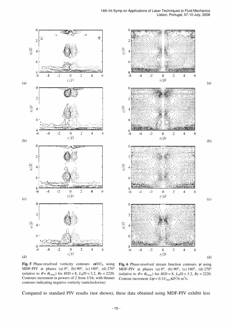
Figures 5 and 6 show phase-resolved flow field results for the same jet conditions (H/D = 8,

L0/D = 3.2, Re = 2220), using MDF-PIV. Four phase angles from 0° to 270° are shown, starting

from the phase of maximum ejection θ = θUmax. As such, the sequence (a-d) shows (a) maximum

ejection, (b) start of suction, (c) maximum suction, (d) start of ejection.

Figure 5 shows contours of dimensionless vorticity ωD/U0, calculated using a circulation-based

algorithm (Raffel et al. 1998). Similar to a free synthetic jet at L0/D = 3 (Shuster and Smith 2007),

each formed vortex propagates far enough from the orifice not to be affected by the suction phase

(starting at (b)). The streamwise distance between consecutive vortices is 3.5D, slightly larger than

L0. The same distance is noted for a free jet. However, the free jet vortices shown by Shuster and

Smith (2007) seem to decay faster than in the present case, although Re is similar. After

impingement, the vortices stretch radially outward, thereby losing strength and decaying into

turbulence. For higher ratios of L0/H (not shown), the vortices remain visible (i.e. phase-resolved)

and sweep across the surface up to r/D > 5.

For the same phases, Fig. 6 shows the stream function contours. Noisy streaks in plots (a-c) are

artefacts from the stream function integration around bad vectors. During maximum suction (c), the

stagnation point (dot) marks the boundary of the fluid sucked into the orifice.


- 10 -

(a)

(b)

(c)

(d)

Fig. 5 Phase-resolved vorticity contours ωD/U0 using

MDF-PIV at phases (a) 0°, (b) 90°, (c) 180°, (d) 270°

(relative to θ = θUmax) for H/D = 8, L0/D = 3.2, Re = 2220.

Contours increment in powers of 2 from 1/16, with thinner

contours indicating negative vorticity (anticlockwise)

(a)

(b)

(c)

(d)

Fig. 6 Phase-resolved stream function contours ψ using

MDF-PIV at phases (a) 0°, (b) 90°, (c) 180°, (d) 270°(relative to θ = θUmax) for H/D = 8, L0/D = 3.2, Re = 2220.

Contour increment ∆ψ = 0.1UmaxπD2/4 m

3/s

Compared to standard PIV results (not shown), these data obtained using MDF-PIV exhibit less


- 11 -

noise in the low velocity regions. As a comparison, Fig. 7 shows contour plots of turbulence

intensities for both techniques. Plots (a,b) on the left are obtained using standard PIV (τ = τmin) and

plots (c,d) on the right are obtained using MDF-PIV with optimal pulse separation. Plots (a,c) and

(b,d) respectively show the time-averaged longitudinal and transversal turbulence intensity u’/U0

and v’/U0.

(a) (c)

(b) (d)

Fig. 7 Contour plots of the time-averaged turbulence intensity, (a,c) longitudinal u’/U0 and (b,d) transversal v’/U0

obtained with (a,b) standard PIV (τ = τmin) and (c,d) MDF-PIV, for H/D = 8, L0/D = 3.2, Re = 2220. Contours increment

in powers of √2 from 1/32

Again, although little difference is notable in the central jet region, MDF-PIV yields less noisy data

in the low velocity regions. In terms of heat transfer, a good resolution of the mean and turbulent

velocity quantities close to the surface is crucial. MDF-PIV has proven useful in that respect.

4. Conclusions

Impinging synthetic jets have been targeted for high heat transfer applications in confined

geometries (Kercher et al. 2003, Gillespie et al. 2006, Pavlova and Amitay 2006). Studying the

relationship between heat transfer and flow dynamics requires an accurate whole-field velocity

measurement technique in a flow field characterised by large differences in velocity magnitude.

A multi-double-frame (MDF) PIV technique is used (Persoons and O’Donovan, in review) which

determines the local optimal pulse separation time based on the maximum of the peak ratio

weighted with the estimated velocity accuracy. At its core, all vector calculations are performed on

double-frame images using state-of-the-art adaptive multipass cross-correlation algorithms with

window shifting and deformation. MDF-PIV improves the measurement accuracy in the low

velocity regions and increases the overall dynamic velocity range (DVR) compared to a

conventional double-frame PIV approach.


- 12 -

Determining the local optimal pulse separation based on the maximum weighted peak ratio requires

minimal user input: (i) an estimated value of the displacement uncertainty ∆s and a suitable choice

of pulse separation multiples (e.g. τ/τmin = {1,8,64}). In practice, MDF-PIV is easily implemented

as an external loop (e.g. as a user-defined macro in LaVision’s DaVis software), and poses no

restrictions either to the vector calculation algorithms or to the hardware.

Using double-frame images, MDF-PIV avoids problems of excessive separation times encountered

with multiframe PIV using single-frame imaging (Hain and Kähler 2007, Pereira et al. 2004). As

such, MDF-PIV is applicable to low and high speed flows. For time-resolved PIV, the flow

frequency content should be lower than the applied camera frame rate. The technique has been

successfully applied for measuring mean and turbulent flow quantities in steady and periodic flows

with arbitrary frequency, as exemplified in this paper and Persoons and O’Donovan (in review)

5. Acknowledgements

The authors acknowledge the financial support of Enterprise Ireland (Grant No. PC/06/191). This

work is performed in the framework of the Centre for Telecommunications Value-Chain Research

(CTVR).

6. References Glezer A, Amitay M (2002) Synthetic jets. Annu Rev Fluid Mech 34:503-529

Kercher DS, Lee JB, Brand O, Allen MG, Glezer A (2003) Microjet cooling devices for thermal management of

electronics. IEEE Trans Comp Packaging Technol 26:359-366

Pavlova A, Amitay M (2006) Electronic cooling using synthetic jet impingement. J Heat Transfer-Trans ASME

128:897-907

Shuster JM, Smith DR (2007) Experimental study of the formation and scaling of a round synthetic jet. Phys Fluids

19:045109

Holman R, Utturkar Y, Mittal R, Smith BL, Cattafesta L (2005) Formation criterion for synthetic jets. AIAA J 43:2110-

2116

Smith BL, Swift GW (2003) A comparison between synthetic jets and continuous jets. Exp Fluids 34:467-472

Gillespie MB, Black WZ, Rinehart C, Glezer A (2006) Local convective heat transfer from a constant heat flux flat

plate cooled by synthetic air jets. J Heat Transfer-Trans ASME 128:990-1000

Persoons T, O’Donovan TS (in review) Improving the local accuracy of particle image velocimetry based on a weighted

peak ratio. Meas Sci Technol

Keane RD, Adrian RJ (1990) Optimization of particle image velocimeters. Part I: Double pulsed systems. Meas Sci

Technol 1:1202-1215

Westerweel J, Dabiri D, Gharib M (1997) The effect of a discrete window offset on the accuracy of cross-correlation

analysis of digital PIV recordings. Exp Fluids 23:20-28

Scarano F (2002) Iterative image deformation methods in PIV. Meas Sci Technol 13:R1-R19

Westerweel J (2008) On velocity gradients in PIV interrogation. Exp Fluids 44:831-842

Westerweel J (2000) Theoretical analysis of the measurement precision in particle image velocimetry. Exp Fluids

(Suppl) 29:S3-S12

Raffel M, Willert C, Kompenhans J (1998) Particle image velocimetry: A practical guide (ed. Adrian RJ et al), Springer,

Berlin

Hain R, Kähler CJ (2007) Fundamentals of multiframe particle image velocimetry (PIV). Exp Fluids 42:575-587

Pereira F, Ciarravano A, Romano GP, Di Felice F (2004) Adaptive multi-frame PIV. In: 12th Int Symp Appl Laser

Techn Fluid Mech, Lisbon, Portugal, July 12-15

Persoons T, O’Donovan TS (2007) A pressure-based estimate of synthetic jet velocity. Phys Fluids 19: 128104

improving the measurement accuracy of piv in a...

Documents