Improving Unsupervised Defect Segmentationby Applying Structural Similarity To Autoencoders

Paul Bergmann1, Sindy Lowe1,2, Michael Fauser1, David Sattlegger1, and Carsten Steger1

1MVTec Software GmbHwww.mvtec.com

{bergmannp,fauser,sattlegger,steger}@mvtec.com

2University of Amsterdamsindy.lowe@student.uva.nl

Abstract—Convolutional autoencoders have emerged as pop-ular methods for unsupervised defect segmentation on imagedata. Most commonly, this task is performed by thresholdinga per-pixel reconstruction error based on an `p-distance.This procedure, however, leads to large residuals wheneverthe reconstruction includes slight localization inaccuraciesaround edges. It also fails to reveal defective regions thathave been visually altered when intensity values stay roughlyconsistent. We show that these problems prevent these ap-proaches from being applied to complex real-world scenar-ios and that they cannot be easily avoided by employingmore elaborate architectures such as variational or featurematching autoencoders. We propose to use a perceptualloss function based on structural similarity that examinesinter-dependencies between local image regions, taking intoaccount luminance, contrast, and structural information,instead of simply comparing single pixel values. It achievessignificant performance gains on a challenging real-worlddataset of nanofibrous materials and a novel dataset of twowoven fabrics over state-of-the-art approaches for unsuper-vised defect segmentation that use per-pixel reconstructionerror metrics.

1. INTRODUCTION

Visual inspection is essential in industrial manufacturingto ensure high production quality and high cost efficiencyby quickly discarding defective parts. Since manual in-spection by humans is slow, expensive, and error-prone,the use of fully automated computer vision systems is be-coming increasingly popular. Supervised methods, wherethe system learns how to segment defective regions bytraining on both defective and non-defective samples, arecommonly used. However, they involve a large effortto annotate data and all possible defect types need tobe known beforehand. Furthermore, in some productionprocesses, the scrap rate might be too small to producea sufficient number of defective samples for training,especially for data-hungry deep learning models.

In this work, we focus on unsupervised defect segmen-tation for visual inspection. The goal is to segment defec-tive regions in images after having trained exclusively onnon-defective samples. It has been shown that architec-

tures based on convolutional neural networks (CNNs) suchas autoencoders (Goodfellow et al., 2016) or generativeadversarial networks (GANs; Goodfellow et al., 2014) canbe used for this task. We provide a brief overview ofsuch methods in Section 2. These models try to recon-struct their inputs in the presence of certain constraintssuch as a bottleneck and thereby manage to capture theessence of high-dimensional data (e.g., images) in a lower-dimensional space. It is assumed that anomalies in the testdata deviate from the training data manifold and the modelis unable to reproduce them. As a result, large reconstruc-tion errors indicate defects. Typically, the error measurethat is employed is a per-pixel `p-distance, which is anad-hoc choice made for the sake of simplicity and speed.However, these measures yield high residuals in locationswhere the reconstruction is only slightly inaccurate, e.g.,due to small localization imprecisions of edges. They alsofail to detect structural differences between the input andreconstructed images when the respective pixels’ colorvalues are roughly consistent. We show that this limits theusefulness of such methods when employed in complexreal-world scenarios.

To alleviate the aforementioned problems, we proposeto measure reconstruction accuracy using the structuralsimilarity (SSIM) metric (Wang et al., 2004). SSIM isa distance measure designed to capture perceptual sim-ilarity that is less sensitive to edge alignment and givesimportance to salient differences between input and re-construction. It captures inter-dependencies between lo-cal pixel regions that are disregarded by the currentstate-of-the-art unsupervised defect segmentation methodsbased on autoencoders with per-pixel losses. We evaluatethe performance gains obtained by employing SSIM asa loss function on two real-world industrial inspectiondatasets and demonstrate significant performance gainsover per-pixel approaches. Figure 1 demonstrates the ad-vantage of perceptual loss functions over a per-pixel `2-loss on the NanoTWICE dataset of nanofibrous materi-als (Carrera et al., 2017). While both autoencoders alterthe reconstruction in defective regions, only the residualmap of the SSIM autoencoder allows a segmentation ofthese areas. By changing the loss function and otherwisekeeping the same autoencoding architecture, we reacha performance that is on par with other state-of-the-art

arX

iv:1

807.

0201

1v3

[cs

.CV

] 1

Feb

201

9

Figure 1: A defective image of nanofibrous materials is reconstructed by an autoencoder optimizing either the commonly usedpixel-wise `2-distance or a perceptual similarity metric based on structural similiarity (SSIM). Even though an `2-autoencoder failsto properly reconstruct the defects, a per-pixel comparison of the original input and reconstruction does not yield significant residualsthat would allow for defect segmentation. The residual map using SSIM puts more importance on the visually salient changes madeby the autoencoder, enabling for an accurate segmentation of the defects.

unsupervised defect segmentation approaches that rely onadditional model priors such as handcrafted features orpretrained networks.

2. RELATED WORK

Detecting anomalies that deviate from the training datahas been a long-standing problem in machine learning.Pimentel et al. (2014) give a comprehensive overview ofthe field. In computer vision, one needs to distinguishbetween two variants of this task. First, there is theclassification scenario, where novel samples appear asentirely different object classes that should be predictedas outliers. Second, there is a scenario where anomaliesmanifest themselves in subtle deviations from otherwiseknown structures and a segmentation of these deviationsis desired. For the classification problem, a number ofapproaches have been proposed (Perera and Patel, 2018;Sabokrou et al., 2018). Here, we limit ourselves to anoverview of methods that attempt to tackle the latterproblem.

Napoletano et al. (2018) extract features from a CNNthat has been pretrained on a classification task. Thefeatures are clustered in a dictionary during training andanomalous structures are identified when the extractedfeatures strongly deviate from the learned cluster centers.General applicability of this approach is not guaranteedsince the pretrained network might not extract usefulfeatures for the new task at hand and it is unclear whichfeatures of the network should be selected for clustering.The results achieved with this method are the current state-of-the-art on the NanoTWICE dataset, which we also usein our experiments. They improve upon previous resultsby Carrera et al. (2017), who build a dictionary that yieldsa sparse representation of the normal data. Similar ap-proaches using sparse representations for novelty detectionare (Boracchi et al., 2014; Carrera et al., 2015, 2016).

Schlegl et al. (2017) train a GAN on optical coherencetomography images of the retina and detect anomaliessuch as retinal fluid by searching for a latent sample thatminimizes the per-pixel `2-reconstruction error as well asa discriminator loss. The large number of optimization

steps that must be performed to find a suitable latentsample makes this approach very slow. Therefore, it isonly useful in applications that are not time-critical. Re-cently, Zenati et al. (2018) proposed to use bidirectionalGANs (Donahue et al., 2017) to add the missing encodernetwork for faster inference. However, GANs are proneto run into mode collapse, i.e., there is no guaranteethat all modes of the distribution of non-defective imagesare captured by the model. Furthermore, they are moredifficult to train than autoencoders since the loss functionof the adversarial training typically cannot be trainedto convergence (Arjovsky and Bottou, 2017). Instead, thetraining results must be judged manually after regularoptimization intervals.

Baur et al. (2018) propose a framework for defectsegmentation using autoencoding architectures and a per-pixel error metric based on the `1-distance. To preventthe disadvantages of their loss function, they improve thereconstruction quality by requiring aligned input data andadding an adversarial loss to enhance the visual quality ofthe reconstructed images. However, for many applicationsthat work on unstructured data, prior alignment is impossi-ble. Furthermore, optimizing for an additional adversarialloss during training but simply segmenting defects basedon per-pixel comparisons during evaluation might leadto worse results since it is unclear how the adversarialtraining influences the reconstruction.

Other approaches take into account the structureof the latent space of variational autoencoders (VAEs;Kingma and Welling, 2014) in order to define measuresfor outlier detection. An and Cho (2015) define a recon-struction probability for every image pixel by drawingmultiple samples from the estimated encoding distributionand measuring the variability of the decoded outputs.Soukup and Pinetz (2018) disregard the decoder outputentirely and instead compute the KL divergence as a nov-elty measure between the prior and the encoder distribu-tion. This is based on the assumption that defective inputswill manifest themselves in mean and variance valuesthat are very different from those of the prior. Similarly,Vasilev et al. (2018) define multiple novelty measures,either by purely considering latent space behavior or by

combining these measures with per-pixel reconstructionlosses. They obtain a single scalar value that indicatesan anomaly, which can quickly become a performancebottleneck in a segmentation scenario where a separateforward pass would be required for each image pixelto obtain an accurate segmentation result. We show thatper-pixel reconstruction probabilities obtained from VAEssuffer from the same problems as per-pixel deterministiclosses (cf. Section 4).

All the aforementioned works that use autoencodersfor unsupervised defect segmentation have shown thatautoencoders reliably reconstruct non-defective imageswhile visually altering defective regions to keep the recon-struction close to the learned manifold of the training data.However, they rely on per-pixel loss functions that makethe unrealistic assumption that neighboring pixel valuesare mutually independent. We show that this preventsthese approaches from segmenting anomalies that differpredominantly in structure rather than pixel intensity. In-stead, we propose to use SSIM (Wang et al., 2004) asthe loss function and measure of anomaly by comparinginput and reconstruction. SSIM takes interdependenciesof local patch regions into account and evaluates theirfirst and second order moments to model differences inluminance, contrast, and structure. Ridgeway et al. (2015)show that SSIM and the closely related multi-scale versionMS-SSIM (Wang et al., 2003) can be used as differen-tiable loss functions to generate more realistic imagesin deep architectures for tasks such as superresolution,but do not examine its usefulness for defect segmentationin an autoencoding framework. In all our experiments,switching from per-pixel to perceptual losses yields sig-nificant gains in performance, sometimes enhancing themethod from a complete failure to a satisfactory defectsegmentation result.

3. METHODOLOGY

3.1. Autoencoders for Unsupervised Defect Seg-mentation

Autoencoders attempt to reconstruct an input imagex ∈ Rk×h×w through a bottleneck, effectively projectingthe input image into a lower-dimensional space, calledlatent space. An autoencoder consists of an encoderfunction E : Rk×h×w → Rd and a decoder functionD : Rd → Rk×h×w, where d denotes the dimensionalityof the latent space and k, h, w denote the number of chan-nels, height, and width of the input image, respectively.Choosing d � k × h × w prevents the architecture fromsimply copying its input and forces the encoder to extractmeaningful features from the input patches that facilitateaccurate reconstruction by the decoder. The overall pro-cess can be summarized as

x = D(E(x)) = D(z) , (1)

where z is the latent vector and x the reconstruction ofthe input. In our experiments, the functions E and D areparameterized by CNNs. Strided convolutions are usedto down-sample the input feature maps in the encoderand to up-sample them in the decoder. Autoencoders canbe employed for unsupervised defect segmentation by

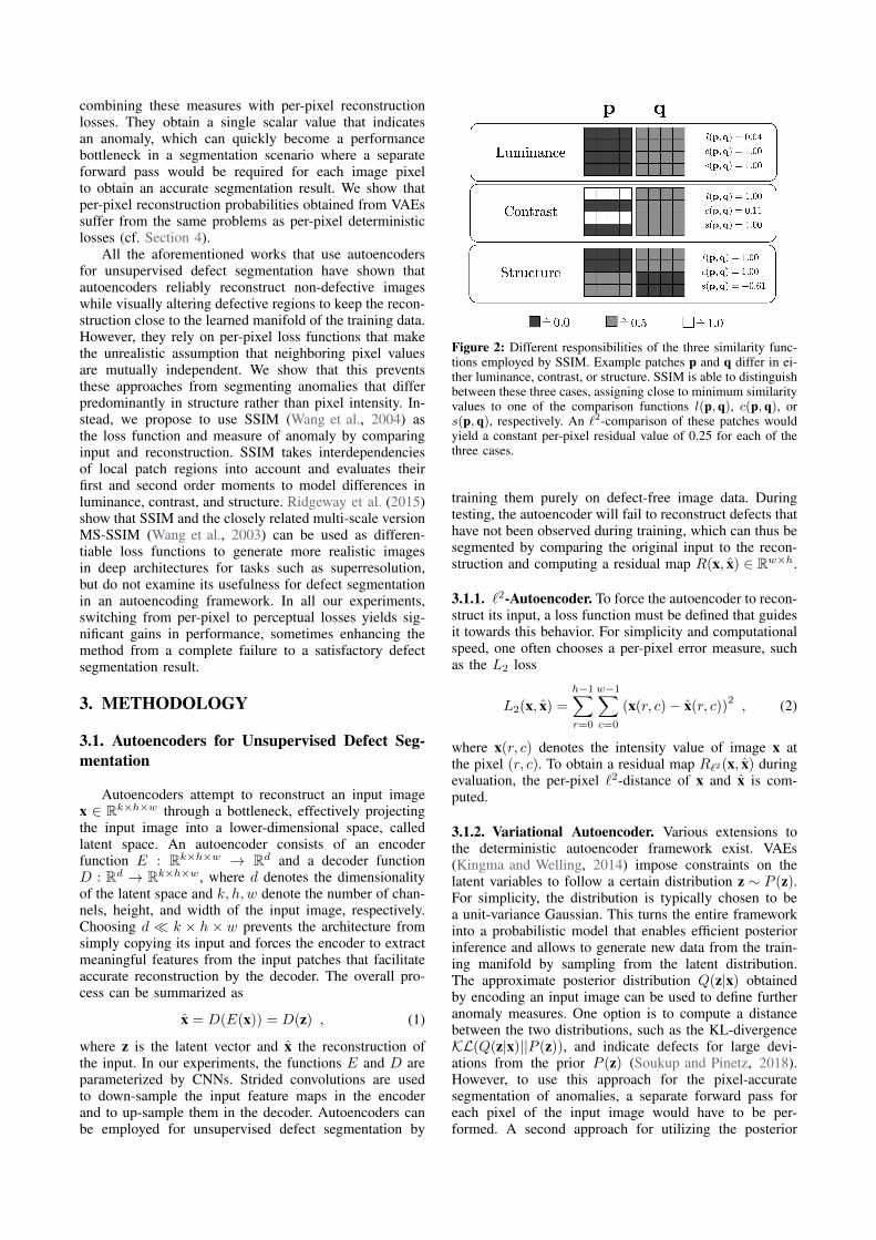
Figure 2: Different responsibilities of the three similarity func-tions employed by SSIM. Example patches p and q differ in ei-ther luminance, contrast, or structure. SSIM is able to distinguishbetween these three cases, assigning close to minimum similarityvalues to one of the comparison functions l(p, q), c(p, q), ors(p, q), respectively. An `2-comparison of these patches wouldyield a constant per-pixel residual value of 0.25 for each of thethree cases.

training them purely on defect-free image data. Duringtesting, the autoencoder will fail to reconstruct defects thathave not been observed during training, which can thus besegmented by comparing the original input to the recon-struction and computing a residual map R(x, x) ∈ Rw×h.

3.1.1. `2-Autoencoder. To force the autoencoder to recon-struct its input, a loss function must be defined that guidesit towards this behavior. For simplicity and computationalspeed, one often chooses a per-pixel error measure, suchas the L2 loss

L2(x, x) =h−1∑r=0

w−1∑c=0

(x(r, c)− x(r, c))2 , (2)

where x(r, c) denotes the intensity value of image x atthe pixel (r, c). To obtain a residual map R`2(x, x) duringevaluation, the per-pixel `2-distance of x and x is com-puted.

3.1.2. Variational Autoencoder. Various extensions tothe deterministic autoencoder framework exist. VAEs(Kingma and Welling, 2014) impose constraints on thelatent variables to follow a certain distribution z ∼ P (z).For simplicity, the distribution is typically chosen to bea unit-variance Gaussian. This turns the entire frameworkinto a probabilistic model that enables efficient posteriorinference and allows to generate new data from the train-ing manifold by sampling from the latent distribution.The approximate posterior distribution Q(z|x) obtainedby encoding an input image can be used to define furtheranomaly measures. One option is to compute a distancebetween the two distributions, such as the KL-divergenceKL(Q(z|x)||P (z)), and indicate defects for large devi-ations from the prior P (z) (Soukup and Pinetz, 2018).However, to use this approach for the pixel-accuratesegmentation of anomalies, a separate forward pass foreach pixel of the input image would have to be per-formed. A second approach for utilizing the posterior

(a) (b) (c) (d)

Figure 3: A toy example illustrating the advantages of SSIM over `2 for the segmentation of defects. (a) 128× 128 checkerboardpattern with gray strokes and dots that simulate defects. (b) Output reconstruction x of the input image x by an `2-autoencodertrained on defect-free checkerboard patterns. The defects have been removed by the autoencoder. (c) `2-residual map. Brighter colorsindicate larger dissimilarity between input and reconstruction. (d) Residuals for luminance l, contrast c, structure s, and their pointwiseproduct that yields the final SSIM residual map. In contrast to the `2-error map, SSIM gives more importance to the visually moresalient disturbances than to the slight inaccuracies around reconstructed edges.

Q(z|x) that yields a spatial residual map is to decode Nlatent samples z1, z2, . . . , zN drawn from Q(z|x) and toevaluate the per-pixel reconstruction probability RV AE =P (x|z1, z2, . . . , zN ) as described by An and Cho (2015).

3.1.3. Feature Matching Autoencoder. Another ex-tension to standard autoencoders was proposed byDosovitskiy and Brox (2016). It increases the quality ofthe produced reconstructions by extracting features fromboth the input image x and its reconstruction x and enforc-ing them to be equal. Consider F : Rk×h×w → Rf to bea feature extractor that obtains an f -dimensional featurevector from an input image. Then, a regularizer can beadded to the loss function of the autoencoder, yieldingthe feature matching autoencoder (FM-AE) loss

LFM(x, x) = L2(x, x) + λ‖F (x)− F (x)‖22 , (3)

where λ > 0 denotes the weighting factor between the twoloss terms. F can be parameterized using the first layers ofa CNN pretrained on an image classification task. Duringevaluation, a residual map RFM is obtained by comparingthe per-pixel `2-distance of x and x. The hope is thatsharper, more realistic reconstructions will lead to betterresidual maps compared to a standard `2-autoencoder.

3.1.4. SSIM Autoencoder. We show that employing moreelaborate architectures such as VAEs or FM-AEs doesnot yield satisfactory improvements of the residial mapsover deterministic `2-autoencoders in the unsuperviseddefect segmentation task. They are all based on per-pixelevaluation metrics that assume an unrealistic indepen-dence between neighboring pixels. Therefore, they fail todetect structural differences between the inputs and theirreconstructions. By adapting the loss and evaluation func-tions to capture local inter-dependencies between imageregions, we are able to drastically improve upon all theaforementioned architectures. In Section 3.2, we specifi-cally motivate the use of the strucutural similarity metricSSIM(x, x) as both the loss function and the evaluationmetric for autoencoders to obtain a residual map RSSIM .

3.2. Structural Similarity

The SSIM index (Wang et al., 2004) defines a distancemeasure between two K × K image patches p and q,taking into account their similarity in luminance l(p,q),contrast c(p,q), and structure s(p,q):

SSIM(p,q) = l(p,q)αc(p,q)βs(p,q)γ , (4)

where α, β, γ ∈ R are user-defined constants to weight thethree terms. The luminance measure l(p,q) is estimatedby comparing the patches’ mean intensities µp and µq.The contrast measure c(p,q) is a function of the patchvariances σ2

p and σ2q . The structure measure s(p,q) takes

into account the covariance σpq of the two patches. Thethree measures are defined as:

l(p,q) =2µpµq + c1µ2

p + µ2q + c1

(5)

c(p,q) =2σpσq + c2σ2

p + σ2q + c2

(6)

s(p,q) =2σpq + c22σpσq + c2

. (7)

The constants c1 and c2 ensure numerical stability and aretypically set to c1 = 0.01 and c2 = 0.03. By substituting(5)-(7) into (4), the SSIM is given by

SSIM(p,q) =(2µpµq + c1)(2σpq + c2)

(µ2p + µ2

q + c1)(σ2p + σ2

q + c2). (8)

It holds that SSIM(p,q) ∈ [−1, 1]. In particular,SSIM(p,q) = 1 if and only if p and q are identical(Wang et al., 2004). Figure 2 shows the different percep-tions of the three similarity functions that form the SSIMindex. Each of the patch pairs p and q has a constant `2-residual of 0.25 per pixel and hence assigns low defectscores to each of the three cases. SSIM on the other handis sensitive to variations in the patches’ mean, variance,and covariance in its respective residual map and assignslow similarity to each of the patch pairs in one of thecomparison functions.

To compute the structural similarity between an entireimage x and its reconstruction x, one slides a K × Kwindow across the image and computes a SSIM value ateach pixel location. Since (8) is differentiable, it can beemployed as a loss function in deep learning architecturesthat are optimized using gradient descent.

Figure 3 indicates the advantages SSIM has over per-pixel error functions such as `2 for segmenting defects.After training an `2-autoencoder on defect-free checker-board patterns of various scales and orientations, we applyit to an image (Figure 3(a)) that contains gray strokesand dots that simulate defects. Figure 3(b) shows the cor-responding reconstruction produced by the autoencoder,which removes the defects from the input image. Thetwo remaining subfigures display the residual maps when

Layer Output Size ParametersKernel Stride Padding

Input 128x128x1Conv1 64x64x32 4x4 2 1Conv2 32x32x32 4x4 2 1Conv3 32x32x32 3x3 1 1Conv4 16x16x64 4x4 2 1Conv5 16x16x64 3x3 1 1Conv6 8x8x128 4x4 2 1Conv7 8x8x64 3x3 1 1Conv8 8x8x32 3x3 1 1Conv9 1x1xd 8x8 1 0

Table 1: General outline of our autoencoder architecture. Thedepicted values correspond to the structure of the encoder. Thedecoder is built as a reversed version of this. Leaky rectifiedlinear units (ReLUs) with slope 0.2 are applied as activationfunctions after each layer except for the output layers of boththe encoder and the decoder, in which linear activation functionsare used.

evaluating the reconstruction error with a per-pixel `2-comparison or SSIM. For the latter, the luminance, con-trast, and structure maps are also shown. For the `2-distance, both the defects and the inaccuracies in thereconstruction of the edges are weighted equally in theerror map, which makes them indistinguishable. SinceSSIM computes three different statistical features for im-age comparison and operates on local patch regions, itis less sensitive to small localization inaccuracies in thereconstruction. In addition, it detects defects that manifestthemselves in a change of structure rather than largedifferences in pixel intensity. For the defects added inthis particular toy example, the contrast function yieldsthe largest residuals.

4. EXPERIMENTS

4.1. Datasets

Due to the lack of datasets for unsupervised defectsegmentation in industrial scenarios, we contribute a noveldataset of two woven fabric textures, which is availableto the public1. We provide 100 defect-free images pertexture for training and validation and 50 images thatcontain various defects such as cuts, roughened areas, andcontaminations on the fabric. Pixel-accurate ground truthannotations for all defects are also provided. All imagesare of size 512× 512 pixels and were acquired as single-channel gray-scale images. Examples of defective anddefect-free textures can be seen in Figure 4. We furtherevaluate our method on a dataset of nanofibrous mate-rials (Carrera et al., 2017), which contains five defect-free gray-scale images of size 1024 × 700 for trainingand validation and 40 defective images for evaluation. Asample image of this dataset is shown in Figure 1.

4.2. Training and Evaluation Procedure

For all datasets, we train the autoencoders with theirrespective losses and evaluation metrics, as described inSection 3.1. Each architecture is trained on 10 000 defect-free patches of size 128×128, randomly cropped from thegiven training images. In order to capture a more globalcontext of the textures, we down-scaled the images to

1. The dataset is available at https://www.mvtec.com/company/research/publications

(a) (b)

(c) (d)

Figure 4: Example images from the contributed texture datasetof two woven fabrics. (a) and (b) show examples of non-defective textures that can be used for training. (c) and (d) showexemplary defects for both datasets. See the text for details.

size 256 × 256 before cropping. Each network is trainedfor 200 epochs using the ADAM (Kingma and Ba, 2015)optimizer with an initial learning rate of 2 × 10−4 anda weight decay set to 10−5. The exact parametrizationof the autoencoder network shared by all tested archi-tectures is given in Table 1. The latent space dimensionfor our experiments is set to d = 100 on the textureimages and to d = 500 for the nanofibres due to theirhigher structural complexity. For the VAE, we decodeN = 6 latent samples from the approximate posteriordistribution Q(z|x) to evaluate the reconstruction proba-bility for each pixel. The feature matching autoencoderis regularized with the first three convolutional layersof an AlexNet (Krizhevsky et al., 2012) pretrained onImageNet (Russakovsky et al., 2015) and a weight factorof λ = 1. For SSIM, the window size is set to K = 11unless mentioned otherwise and its three residual mapsare equally weighted by setting α = β = γ = 1.

The evaluation is performed by striding over the testimages and reconstructing image patches of size 128×128using the trained autoencoder and computing its respectiveresidual map R. In principle, it would be possible to set thehorizontal and vertical stride to 128. However, at differentspatial locations, the autoencoder produces slightly differ-ent reconstructions of the same data, which leads to somestriding artifacts. Therefore, we decreased the stride to 30pixels and averaged the reconstructed pixel values. Theresulting residual maps are thresholded to obtain candidateregions where a defect might be present. An opening witha circular structuring element of diameter 4 is applied asa morphological post-processing to delete outlier regionsthat are only a few pixels wide (Steger et al., 2018). Wecompute the receiver operating characteristic (ROC) asthe evaluation metric. The true positive rate is defined asthe ratio of pixels correctly classified as defect across theentire dataset. The false positive rate is the ratio of pixelsmisclassified as defect.

Figure 5: Qualitative comparison between reconstructions, residual maps, and segmentation results of an `2-autoencoder and anSSIM autoencoder on two datasets of woven fabric textures. The ground truth regions containing defects are outlined in red whilegreen areas mark the segmentation result of the respective method.

(a) (b) (c)

Figure 6: Resulting ROC curves of the proposed SSIM autoencoder (red line) on the evaluated datasets of nanofibrous materials (a)and the two texture datasets (b), (c) in comparison with other autoencoding architectures that use per-pixel loss functions (green,orange, and blue lines). Corresponding AUC values are given in the legend.

4.3. Results

Figure 5 shows a qualitative comparison between theperformance of the `2-autoencoder and the SSIM autoen-coder on images of the two texture datasets. Although botharchitectures remove the defect in the reconstruction, onlythe SSIM residual map reveals the defects and provides anaccurate segmentation result. The same can be observedfor the NanoTWICE dataset, as shown in Figure 1.

We confirm this qualitative behavior by numericalresults. Figure 6 compares the ROC curves and theirrespective AUC values of our approach using SSIM tothe per-pixel architectures. The performance of the latteris often only marginally better than classifying each pixelrandomly. For the VAE, we found that the reconstructionsobtained by different latent samples from the posteriordoes not vary greatly. Thus, it could not improve onthe deterministic framework. Employing feature matchingonly improved the segmentation result for the dataset ofnanofibrous materials, while not yielding a benefit forthe two texture datasets. Using SSIM as the loss andevaluation metric outperforms all other tested architecturessignificantly. By merely changing the loss function, theachieved AUC improves from 0.688 to 0.966 on thedataset of nanofibrous materials, which is comparableto the state-of-the-art by Napoletano et al. (2018), wherevalues of up to 0.974 are reported. In contrast to thismethod, autoencoders do not rely on any model priors

such as handcrafted features or pretrained networks. Forthe two texture datasets, similar leaps in performance areobserved.

Since the dataset of nanofibrous materials containsdefects of various sizes and smaller sized defects con-tribute less to the overall true positive rate when weight-ing all pixel equally, we further evaluated the over-lap of each detected anomaly region with the groundtruth for this dataset and report the p-quantiles for p ∈{25%, 50%, 75%} in Figure 7. For false positive ratesas low as 5%, more than 50% of the defects have anoverlap with the ground truth that is larger than 91%.This outperforms the results achieved by Napoletano et al.(2018), who report a minimal overlap of 85% in thissetting.

We further tested the sensitivity of the SSIM au-toencoder to different hyperparameter settings. We variedthe latent space dimension d, SSIM window size k, andthe size of the patches that the autoencoder was trainedon. Table 2 shows that SSIM is insensitive to differenthyperparameter settings once the latent space dimensionis chosen to be sufficiently large. Using the optimal setupof d = 500, k = 11, and patch size 128 × 128, aforward pass through our architecture takes 2.23 ms on aTesla V100 GPU. Patch-by-patch evaluation of an entireimage of the NanoTWICE dataset takes 3.61 s on average,which is significantly faster than the runtimes reported byNapoletano et al. (2018). Their approach requires between

0.0 0.1 0.2 0.3False Positive Rate

0.0

0.2

0.4

0.6

0.8

1.0Ov

erla

p

25-quantile50-quantile75-quantile

Figure 7: Per-region overlap for individual defects between oursegmentation and the ground truth for different false positiverates using an SSIM autoencoder on the dataset of nanofibrousmaterials.

15 s and 55 s to process a single input image.Figure 8 depicts qualitative advantages that employing

a perceptual error metric has over per-pixel distances suchas `2. It displays two defective images from one of thetexture datasets, where the top image contains a high-contrast defect of metal pins which contaminate the fabric.The bottom image shows a low-contrast structural defectwhere the fabric was cut open. While the `2-norm hasproblems to detect the low-constrast defect, it easily seg-ments the metal pins due to their large absolute distancein gray values with respect to the background. However,misalignments in edge regions still lead to large residualsin non-defective regions as well, which would make thesethin defects hard to segment in practice. SSIM robustlysegments both defect types due to its simultaneous focuson luminance, contrast, and structural information andinsensitivity to edge alignment due to its patch-by-patchcomparisons.

5. CONCLUSION

We demonstrate the advantage of perceptual loss func-tions over commonly used per-pixel residuals in autoen-coding architectures when used for unsupervised defectsegmentation tasks. Per-pixel losses fail to capture inter-dependencies between local image regions and thereforeare of limited use when defects manifest themselves instructural alterations of the defect-free material wherepixel intensity values stay roughly consistent. We furthershow that employing probabilistic per-pixel error metricsobtained by VAEs or sharpening reconstructions by fea-ture matching regularization techniques do not improvethe segmentation result since they do not address theproblems that arise from treating pixels as mutually in-dependent.

SSIM, on the other hand, is less sensitive to small in-accuracies of edge locations due to its comparison of localpatch regions and takes into account three different sta-tistical measures: luminance, contrast, and structure. Wedemonstrate that switching from per-pixel loss functionsto an error metric based on structural similarity yieldssignificant improvements by evaluating on a challengingreal-world dataset of nanofibrous materials and a con-tributed dataset of two woven fabric materials which wemake publicly available. Employing SSIM often achievesan enhancement from almost unusable segmentations toresults that are on par with other state of the art approaches

Latentdimension AUC SSIM

window size AUC Patch size AUC

50 0.848 3 0.889100 0.935 7 0.965 32 0.949200 0.961 11 0.966 64 0.959500 0.966 15 0.960 128 0.9661000 0.962 19 0.952

Table 2: Area under the ROC curve (AUC) on NanoTWICE forvarying hyperparameters in the SSIM autoencoder architecture.Different settings do not significantly alter defect segmentationperformance.

Figure 8: In the first row, the metal pins have a large differencein gray values in comparison to the defect-free backgroundmaterial. Therefore, they can be detected by both the `2 andthe SSIM error metric. The defect shown in the second row,however, differs from the texture more in terms of structure thanin absolute gray values. As a consequence, a per-pixel distancemetric fails to segment the defect while SSIM yields a goodsegmentation result.

for unsupervised defect segmentation which additionallyrely on image priors such as pre-trained networks.

References

Jinwon An and Sungzoon Cho. Variational Autoencoderbased Anomaly Detection using Reconstruction Proba-bility. SNU Data Mining Center, Tech. Rep., 2015.

Martin Arjovsky and Leon Bottou. Towards PrincipledMethods for Training Generative Adversarial Networks.International Conference on Learning Representations,2017.

Christoph Baur, Benedikt Wiestler, Shadi Albarqouni, andNassir Navab. Deep Autoencoding Models for Unsu-pervised Anomaly Segmentation in Brain MR Images.arXiv preprint arXiv:1804.04488, 2018.

Giacomo Boracchi, Diego Carrera, and Brendt Wohlberg.Novelty Detection in Images by Sparse Representations.In 2014 IEEE Symposium on Intelligent EmbeddedSystems (IES), pages 47–54. IEEE, 2014.

Diego Carrera, Giacomo Boracchi, Alessandro Foi, andBrendt Wohlberg. Detecting anomalous structures byconvolutional sparse models. In 2015 InternationalJoint Conference on Neural Networks (IJCNN), pages1–8. IEEE, 2015.

Diego Carrera, Giacomo Boracchi, Alessandro Foi, andBrendt Wohlberg. Scale-invariant anomaly detectionwith multiscale group-sparse models. In 2016 IEEEInternational Conference on Image Processing (ICIP),pages 3892–3896. IEEE, 2016.

Diego Carrera, Fabio Manganini, Giacomo Boracchi, andEttore Lanzarone. Defect Detection in SEM Images ofNanofibrous Materials. IEEE Transactions on IndustrialInformatics, 13(2):551–561, 2017.

Jeff Donahue, Philipp Krahenbuhl, and Trevor Darrell.Adversarial Feature Learning. International Conferenceon Learning Representations, 2017.

Alexey Dosovitskiy and Thomas Brox. Generating Imageswith Perceptual Similarity Metrics based on Deep Net-works. In Advances in Neural Information ProcessingSystems, pages 658–666, 2016.

Ian Goodfellow, Jean Pouget-Abadie, Mehdi Mirza,Bing Xu, David Warde-Farley, Sherjil Ozair, AaronCourville, and Yoshua Bengio. Generative AdversarialNets. In Advances in Neural Information ProcessingSystems, pages 2672–2680, 2014.

Ian Goodfellow, Yoshua Bengio, and Aaron Courville.Deep Learning. MIT Press, 2016.

Diederik P Kingma and Jimmy Ba. Adam: A Method forStochastic Optimization. International Conference onLearning Representations, 2015.

Diederik P Kingma and Max Welling. Auto-EncodingVariational Bayes. International Conference on Learn-ing Representations, 2014.

Alex Krizhevsky, Ilya Sutskever, and Geoffrey E Hin-ton. ImageNet Classification With Deep ConvolutionalNeural Networks. In Advances in Neural InformationProcessing Systems, pages 1097–1105, 2012.

Paolo Napoletano, Flavio Piccoli, and Raimondo Schet-tini. Anomaly Detection in Nanofibrous Materials byCNN-Based Self-Similarity. Sensors, 18(1):209, 2018.

Pramuditha Perera and Vishal M Patel. Learning DeepFeatures for One-Class Classification. arXiv preprintarXiv:1801.05365, 2018.

Marco AF Pimentel, David A Clifton, Lei Clifton, andLionel Tarassenko. A review of novelty detection.Signal Processing, 99:215–249, 2014.

Karl Ridgeway, Jake Snell, Brett Roads, Richard S Zemel,and Michael C Mozer. Learning to generate im-ages with perceptual similarity metrics. arXiv preprintarXiv:1511.06409, 2015.

Olga Russakovsky, Jia Deng, Hao Su, Jonathan Krause,Sanjeev Satheesh, Sean Ma, Zhiheng Huang, AndrejKarpathy, Aditya Khosla, Michael Bernstein, et al.ImageNet Large Scale Visual Recognition Challenge.International Journal of Computer Vision, 115(3):211–252, 2015.

Mohammad Sabokrou, Mohammad Khalooei, MahmoodFathy, and Ehsan Adeli. Adversarially Learned One-Class Classifier for Novelty Detection. In Proceedingsof the IEEE Conference on Computer Vision and Pat-tern Recognition, pages 3379–3388, 2018.

Thomas Schlegl, Philipp Seebock, Sebastian M Waldstein,Ursula Schmidt-Erfurth, and Georg Langs. Unsuper-vised Anomaly Detection with Generative AdversarialNetworks to Guide Marker Discovery. In Interna-tional Conference on Information Processing in Medi-cal Imaging, pages 146–157. Springer, 2017.

Daniel Soukup and Thomas Pinetz. Reliably DecodingAutoencoders Latent Spaces for One-Class LearningImage Inspection Scenarios. In OAGM Workshop 2018.Verlag der Technischen Universitat Graz, 2018.

Carsten Steger, Markus Ulrich, and Christian Wiedemann.Machine Vision Algorithms and Applications. Wiley-VCH, Weinheim, 2nd edition, 2018.

Aleksei Vasilev, Vladimir Golkov, Ilona Lipp, EleonoraSgarlata, Valentina Tomassini, Derek K Jones, and

Daniel Cremers. q-Space Novelty Detection with Varia-tional Autoencoders. arXiv preprint arXiv:1806.02997,2018.

Zhou Wang, Eero P Simoncelli, and Alan C Bovik. Multi-scale structural similarity for image quality assessment.In Record of the Thirty-Seventh Asilomar Conferenceon Signals, Systems and Computers, volume 2, pages1398–1402. IEEE, 2003.

Zhou Wang, Alan C Bovik, Hamid R Sheikh, and Eero PSimoncelli. Image quality assessment: from error vis-ibility to structural similarity. IEEE transactions onimage processing, 13(4):600–612, 2004.

Houssam Zenati, Chuan Sheng Foo, Bruno Lecouat, Gau-rav Manek, and Vijay Ramaseshan Chandrasekhar. Ef-ficient GAN-Based Anomaly Detection. arXiv preprintarXiv:1802.06222, 2018.