imsl fortran library user’s guide math/library special ... · imsl math/library special functions...
TRANSCRIPT
Mathematical Functions in Fortran
IMSL Fortran Library User’s GuideMATH/LIBRARY Special Functions
Trusted For Over Years30

Mathematical Functions in Fortran
IMSL MATH/LIBRARY User’s GuideSpecial Functions
P/N 7681 [ w w w . v n i . c o m ]
Visual Numerics, Inc. � United States Corporate Headquarters 2000 Crow Canyon Place, Suite 270 San Ramon, CA 94583 PHONE: 925-807-0138 FAX: 925-807-0145 e-mail: [email protected] Westminster, CO PHONE: 303-379-3040 Houston, TX PHONE: 713-784-3131
Visual Numerics International Ltd. Centennial Court Easthampstead Road Bracknell, Berkshire RG12 1YQ UNITED KINGDOM PHONE: +44 (0) 1344-458700 FAX: +44 (0) 1344-458748 e-mail: [email protected]
Visual Numerics SARL Immeuble le Wilson 1 70, avenue due General de Gaulle F-92058 PARIS LA DEFENSE, Cedex FRANCE PHONE: +33-1-46-93-94-20 FAX: +33-1-46-93-94-39 e-mail: [email protected]
Visual Numerics S. A. de C. V. Florencia 57 Piso 10-01 Col. Juarez Mexico D. F. C. P. 06600 MEXICO PHONE: +52-55-514-9730 or 9628 FAX: +52-55-514-4873
Visual Numerics International GmbH Zettachring 10 D-70567Stuttgart GERMANY PHONE: +49-711-13287-0 FAX: +49-711-13287-99 e-mail: [email protected]
Visual Numerics Japan, Inc. GOBANCHO HIKARI BLDG. 4TH Floor 14 GOBAN-CHO CHIYODA-KU TOKYO, JAPAN 102 PHONE: +81-3-5211-7760 FAX: +81-3-5211-7769 e-mail: [email protected]
Visual Numerics, Inc. 7/F, #510, Sect. 5 Chung Hsiao E. Road Taipei, Taiwan 110 ROC PHONE: +(886) 2-2727-2255 FAX: +(886) 2-2727-6798 e-mail: [email protected]
Visual Numerics Korea, Inc. HANSHIN BLDG. Room 801 136-1, MAPO-DONG, MAPO-GU SEOUL, 121-050 KOREA SOUTH PHONE: +82-2-3273-2632 or 2633 FAX: +82-2-3273--2634 e-mail: [email protected]
World Wide Web site: http://www.vni.com
COPYRIGHT NOTICE: Copyright 1994-2003 by Visual Numerics, Inc. All rights reserved. Unpublished�rights reserved under the copyright laws of the United States. Printed in the USA.
The information contained in this document is subject to change without notice.
This document is provided AS IS, with NO WARRANTY. VISUAL NUMERICS, INC., SHALL NOT BE LIABLE FOR ANY ERRORS WHICH MAY BE CONTAINED HEREIN OR FOR INCIDENTAL, CONSEQUENTIAL, OR OTHER INDIRECT DAMAGES IN CONNECTION WITH THE FURNISHING, PERFORMANCE OR USE OF THIS MATERIAL. [Carol: note case change]
IMSL, PV- WAVE, and Visual Numerics are registered in the U.S. Patent and Trademark Office by, and PV- WAVE Advantage is a trademark of, Visual Numerics, Inc.
TRADEMARK NOTICE: The following are trademarks or registered trademarks of their respective owners, as follows: Microsoft, Windows, Windows 95, Windows NT, Internet Explorer � Microsoft Corporation; Motif � The Open Systems Foundation, Inc.; PostScript � Adobe Systems, Inc.; UNIX � X/Open Company, Limited; X Window System, X11 � Massachusetts Institute of Technology; RISC System/6000 and IBM � International Business Machines Corporation; Sun, Java, JavaBeans � Sun Microsystems, Inc.; JavaScript, Netscape Communicator � Netscape, Inc.; HPGL and PCL � Hewlett Packard Corporation; DEC, VAX, VMS, OpenVMS � Compaq Information Technologies Group, L.P./Hewlett Packard Corporation; Tektronix 4510 Rasterizer � Tektronix, Inc.; IRIX, TIFF � Silicon Graphics, Inc.; SPARCstation � SPARC International, licensed exclusively to Sun Microsystems, Inc.; HyperHelp � Bristol Technology, Inc. Other products and company names mentioned herein are trademarks of their respective owners.
Use of this document is governed by a Visual Numerics Software License Agreement. This document contains confidential and proprietary information. No part of this document may be reproduced or transmitted in any form without the prior written consent of Visual Numerics.
RESTRICTED RIGHTS NOTICE: This documentation is provided with RESTRICTED RIGHTS. Use, duplication or disclosure by the US Government is subject to restrictions as set forth in subparagraph (c)(1)(ii) of the Rights in Technical Data and Computer Software clause at DFAR 252.227-7013, and in subparagraphs (a) through (d) of the Commercial Computer software � Restricted Rights clause at FAR 52.227-19, and in similar clauses in the NASA FAR Supplement, when applicable. Contractor/Manufacturer is Visual Numerics, Inc., 2500 Wilcrest Drive, Suite 200, Houston, TX 77042-2759.
IMSL Fortran, C, and Java Application Development Tools

IMSL MATH/LIBRARY Special Functions Contents � i
Contents
Introduction vii
Chapter 1: Elementary Functions 1
Chapter 2: Trigonometric and Hyperbolic Functions 9
Chapter 3: Exponential Integrals and Related Functions 31
Chapter 4: Gamma Function and Related Functions 47
Chapter 5: Error Function and Related Functions 75
Chapter 6: Bessel Functions 91
Chapter 7: Kelvin Functions 133
Chapter 8: Airy Functions 149
Chapter 9: Elliptic Integrals 161
Chapter 10: Elliptic and Related Functions 173
Chapter 11: Probability Distribution Functions and Inverses 185
Chapter 12: Mathieu Functions 241
Chapter 13: Miscellaneous Functions 253
ii � Contents IMSL MATH/LIBRARY Special Functions
Reference Material 259
GAMS Index A-1
Alphabetical Summary of Routines B-1
Appendix C: References C-1
Product Support i
Index iii
IMSL MATH/LIBRARY Special Functions Introduction � vii
Introduction
The IMSL Fortran Libraries The IMSL Libraries consist of two separate, but coordinated Libraries that allow easy user access. These Libraries are organized as follows:
� MATH/LIBRARY general applied mathematics and special functions
The User�s Guide for IMSL MATH/LIBRARY has two parts:
1. MATH/LIBRARY (Volumes 1 and 2)
2. MATH/LIBRARY Special Functions
� STAT/LIBRARY statistics
Most of the routines are available in both single and double precision versions. Many routines are also available for complex and complex-double precision arithmetic. The same user interface is found on the many hardware versions that span the range from personal computer to supercomputer. Note that some IMSL routines are not distributed for FORTRAN compiler environments that do not support double precision complex data. The specific names of the IMSL routines that return or accept the type double complex begin with the letter �Z� and, occasionally, �DC.�
Getting Started IMSL MATH/LIBRARY Special Functions is a collection of FORTRAN subroutines and functions useful in research and statistical analysis. Each routine is designed and documented to be used in research activities as well as by technical specialists.
To use any of these routines, you must write a program in FORTRAN (or possibly some other language) to call the MATH/LIBRARY Special Functions routine. Each routine conforms to established conventions in programming and documentation. We give first priority in development to efficient algorithms, clear documentation, and accurate results. The uniform design of the routines makes it easy to use more than one routine in a given application. Also, you will find that the design consistency enables you to apply your experience with one MATH/LIBRARY Special Functions routine to all other IMSL routines that you use.
viii � Introduction IMSL MATH/LIBRARY Special Functions
Finding the Right Routine The organization of IMSL MATH/LIBRARY Special Functions closely parallels that of the National Bureau of Standards� Handbook of Mathematical Functions, edited by Abramowitz and Stegun (1964). Corresponding to the NBS Handbook, functions are arranged into separate chapters, such as elementary functions, trigonometric and hyperbolic functions, exponential integrals, gamma function and related functions, and Bessel functions. To locate the right routine for a given problem, you may use either the table of contents located in each chapter introduction, or one of the indexes at the end of this manual. GAMS index uses GAMS classification (Boisvert, R.F., S.E. Howe, D.K. Kahaner, and J.L. Springmann 1990, Guide to Available Mathematical Software, National Institute of Standards and Technology NISTIR 90-4237). Use the GAMS index to locate which MATH/LIBRARY Special Functions routines pertain to a particular topic or problem.
Organization of the Documentation This manual contains a concise description of each routine, with at least one demonstrated exam-ple of each routine, including sample input and results. You will find all information pertaining to the Special Functions Library in this manual. Moreover, all information pertaining to a particular routine is in one place within a chapter.
Each chapter begins with an introduction followed by a table of contents that lists the routines included in the chapter. Documentation of the routines consists of the following information:
� IMSL Routine�s Generic Name
� Purpose: a statement of the purpose of the routine. If the routine is a function rather than a subroutine the purpose statement will reflect this fact.
� Function Return Value: a description of the return value (for functions only).
� Required Arguments: a description of the required arguments in the order of their occurrence. Input arguments usually occur first, followed by input/output arguments, with output arguments described last. Futhermore, the following terms apply to arguments:
Input Argument must be initialized; it is not changed by the routine.
Input/Output Argument must be initialized; the routine returns output through this argument; cannot be a constant or an expression.
Input or Output Select appropriate option to define the argument as either input or output. See individual routines for further instructions.
Output No initialization is necessary; cannot be a constant or an expression. The routine returns output through this argument.
� Optional Arguments: a description of the optional arguments in the order of their occurrence.
� Fortran 90 Interface: a section that describes the generic and specific interfaces to the routine.
� Fortran 77 Style Interfaces: an optional section, which describes Fortran 77 style interfaces, is supplied for backwards compatibility with previous versions of the Library.
IMSL MATH/LIBRARY Special Functions Introduction � ix
� Example: at least one application of this routine showing input and required dimension and type statements.
� Output: results from the example.
� Comments: details pertaining to code usage.
� Description: a description of the algorithm and references to detailed information. In many cases, other IMSL routines with similar or complementary functions are noted.
� Programming notes: an optional section that contains programming details not covered elsewhere.
� References: periodicals and books with details of algorithm development.
� Additional Examples: an optional section with additional applications of this routine showing input and required dimension and type statements.
Naming Conventions The names of the routines are mnemonic and unique. Most routines are available in both a single precision and a double precision version, with names of the two versions sharing a common root. The root name is also the generic interface name. The name of the double precision specific version begins with a �D_.� The single precision specific version begins with an �S_�. For example, the following pairs are precision specific names of routines in the two different precisions: S_GAMDF/D_GAMDF (the root is �GAMDF ,� for �Gamma distribution function�) and S_POIDF/D_POIDF (the root is �POIDF,� for �Poisson distribution function�). The precision specific names of the IMSL routines that return or accept the type complex data begin with the letter �C_� or �Z_� for complex or double complex, respectively. Of course the generic name can be used as an entry point for all precisions supported.
When this convention is not followed the generic and specific interfaces are noted in the documentation. For example, in the case of the BLAS and trigonometric intrinsic functions where standard names are already established, the standard names are used as the precision specific names. There may also be other interfaces supplied to the routine to provide for backwards compatibility with previous versions of the Library. These alternate interfaces are noted in the documentation when they are available.
Except when expressly stated otherwise, the names of the variables in the argument lists follow the FORTRAN default type for integer and floating point. In other words, a variable whose name begins with one of the letters �I� through �N� is of type INTEGER, and otherwise is of type REAL or DOUBLE PRECISION, depending on the precision of the routine.
An assumed-size array with more than one dimension that is used as a FORTRAN argument can have an assumed-size declarator for the last dimension only. In the MATH/LIBRARY Special Functions routines, the information about the first dimension is passed by a variable with the prefix �LD� and with the array name as the root. For example, the argument LDA contains the leading dimension of array A. In most cases, information about the dimensions of arrays is obtained from the array through the use of Fortran 90�s size function. Therefore, arguments carrying this type of information are usually defined as optional arguments.
Where appropriate, the same variable name is used consistently throughout a chapter in the MATH/LIBRARY Special Functions. For example, in the routines for random number generation,
x � Introduction IMSL MATH/LIBRARY Special Functions
NR denotes the number of random numbers to be generated, and R or IR denotes the array that stores the numbers.
When writing programs accessing the MATH/LIBRARY Special Functions , the user should choose FORTRAN names that do not conflict with names of IMSL subroutines, functions, or named common blocks. The careful user can avoid any conflicts with IMSL names if, in choosing names, the following rules are observed:
� Do not choose a name that appears in the Alphabetical Summary of Routines, at the end of the User�s Manual, nor one of these names preceded by a D, S_, D_, C_, or Z_.
� Do not choose a name consisting of more than three characters with a numeral in the second or third position.
For further details, see the section on �Reserved Names� in the Reference Material.
Using Library Subprograms The documentation for the routines uses the generic name and omits the prefix, and hence the entire suite of routines for that subject is documented under the generic name.
Examples that appear in the documentation also use the generic name. To further illustrate this principle, note the BSJNS documentation (see Chapter 6, Bessel Functions, of this manual). A description is provided for just one data type. There are four documented routines in this subject area: S_BSJNS, D_BSJNS, C_BSJNS, and Z_BSJNS.
These routines constitute single-precision, double-precision, complex, and complex double-precision versions of the code.
The appropriate routine is identified by the Fortran 90 compiler. Use of a module is required with the routines. The naming convention for modules joins the suffix �_int� to the generic routine name. Thus, the line �use BSJNS_INT� is inserted near the top of any routine that calls the subprogram �BSJNS�. More inclusive modules are also available. For example, the module named �imsl_libraries� contains the interface modules for all routines in the library.
When dealing with a complex matrix, all references to the transpose of a matrix, AT , are replaced by the adjoint matrix
A A AT H� �
� where the overstrike denotes complex conjugation. IMSL Fortran Library linear algebra software uses this convention to conserve the utility of generic documentation for that code subject. References to orthogonal matrices are replaced by their complex counterparts, unitary matrices. Thus, an n � n orthogonal matrix Q satisfies the condition Q Q IT
n� . An n � n unitary matrix V satisfies the analogous condition for complex matrices, V V In
*� .
Programming Conventions In general, the IMSL MATH/LIBRARY Special Functions codes are written so that computations are not affected by underflow, provided the system (hardware or software) places a zero value in the register. In this case, system error messages indicating underflow should be ignored.
IMSL MATH/LIBRARY Special Functions Introduction � xi
IMSL codes also are written to avoid overflow. A program that produces system error messages indicating overflow should be examined for programming errors such as incorrect input data, mismatch of argument types, or improper dimensioning.
In many cases, the documentation for a routine points out common pitfalls that can lead to failure of the algorithm.
Library routines detect error conditions, classify them as to severity, and treat them accordingly. This error-handling capability provides automatic protection for the user without requiring the user to make any specific provisions for the treatment of error conditions. See the section on �User Errors� in the Reference Material for further details.
Module Usage Users are required to incorporate a �use� statement near the top of their program for the IMSL routine being called when writing new code that uses this library. However, legacy code which calls routines in the previous version of the library without the presence of a �use� statement will continue to work as before. The example programs throughout this manual demonstrate the syntax for including use statements in your program. In addition to the examples programs, common cases of when and how to employ a use statement are described below.
�� Users writing new programs calling the generic interface to IMSL routines must include a use statement near the top of any routine that calls the IMSL routines. The naming convention for modules joins the suffix �_int� to the generic routine name. For example, if a new program is written calling the IMSL routines LFTRG and LFSRG, then the following use statements should be inserted inserted near the top of the program USE LFTRG_INT USE LFSRG_INT
In addition to providing interface modules for each routine individually, we also provide a module named �imsl_libraries�, which contains the generic interfaces for all routines in the library. For programs that call several different IMSL routines using generic interfaces, it can be simpler to insert the line USE IMSL_LIBRARIES
rather than list use statements for every IMSL subroutine called.
�� Users wishing to update existing programs to call other routines from this library should incorporate a use statement for the new routine being called. (Here, the term �new routine� implies any routine in the library, only �new� to the user�s program.) For example, if a call to the generic interface for the routine LSARG is added to an existing program, then USE LSARG_INT
should be inserted near the top of your program.
�� Users wishing to update existing programs to call the new generic versions of the routines must change their calls to the existing routines to match the new calling sequences and use either the routine specific interface modules or the all encompassing �imsl_libraries� module.
xii � Introduction IMSL MATH/LIBRARY Special Functions
�� Code which employed the �use numerical_libraries� statement from the previous version of the library will continue to work properly with this version of the library.
Programming Tips It is strongly suggested that users force all program variables to be explicitly typed. This is done by including the line �IMPLICIT NONE� as close to the first line as possible. Study some of the examples accompanying an IMSL Fortran Library routine early on. These examples are available online as part of the product.
Each subject routine called or otherwise referenced requires the �use� statement for an interface block designed for that subject routine. The contents of this interface block are the interfaces to the separate routines available for that subject. Packaged descriptive names for option numbers that modify documented optional data or internal parameters might also be provided in the interface block. Although this seems like an additional complication, many typographical errors are avoided at an early stage in development through the use of these interface blocks. The �use� statement is required for each routine called in the user�s program.
However, if one is only using the Fortran 77 interfaces supplied for backwards compatibility then the �use� statements are not required.
Optional Subprogram Arguments IMSL Fortran Library routines have required arguments and may have optional arguments. All arguments are documented for each routine. For example, consider the routine GCIN that evaluates the inverse of a general continuous CDF. The required arguments are P, X, and F. The optional arguments are IOPT and M. Both IOPT and M take on default values so are not required as input by the user unless the user wishes for these arguments to take on some value other than the default. Often there are other output arguments that are listed as optional because although they may contain information that is closely connected with the computation they are not as compelling as the primary problem. In our example code, GCIN, if the user wishes to input the optional argument �IOPT� then the use of the keyword �IOPT=� in the argument list to assign an input value to IOPT would be necessary.
For compatibility with previous versions of the IMSL Libraries, the NUMERICAL_LIBRARIES interface module includes backwards compatible positional argument interfaces to all routines which existed in the Fortran 77 version of the Library. Note that it is not necessary to use �use� statements when calling these routines by themselves. Existing programs which called these routines will continue to work in the same manner as before.
Error Handling The routines in IMSL MATH/LIBRARY Special Functions attempt to detect and report errors and invalid input. Errors are classified and are assigned a code number. By default, errors of moderate or worse severity result in messages being automatically printed by the routine. Moreover, errors of worse severity cause program execution to stop. The severity level as well as the general nature of the error is designated by an �error type� with numbers from 0 to 5. An error type 0 is no error; types 1 through 5 are progressively more severe. In most cases, you need not be concerned with
IMSL MATH/LIBRARY Special Functions Introduction � xiii
our method of handling errors. For those interested, a complete description of the error-handling system is given in the Reference Material, which also describes how you can change the default actions and access the error code numbers.
Printing Results None of the routines in IMSL MATH/LIBRARY Special Functions print results (but error messages may be printed). The output is returned in FORTRAN variables, and you can print these yourself.
The IMSL routine UMACH (see the Reference Material section of this manual) retrieves the FORTRAN device unit number for printing. Because this routine obtains device unit numbers, it can be used to redirect the input or output. The section on �Machine-Dependent Constants� in the Reference Material contains a description of the routine UMACH.


IMSL MATH/LIBRARY Special Functions Chapter 1: Elementary Functions � 1
Chapter 1: Elementary Functions
Routines Evaluates the argument of a complex number ......................CARG 1 Evaluates the cube root of a real or complex number 3 x .... CBRT 2 Evaluates (ex � 1)/x for real or complex x ........................... EXPRL 3 Evaluates the complex base 10 logarithm, log�� z ............... LOG10 5 Evaluates ln(x + 1) for real or complex x ...........................ALNREL 6
Usage Notes The �relative� function EXPRL (page 3) is useful for accurately computing ex � 1 near x = 0. Computing ex � 1 using EXP(X) ��1 near x = 0 is subject to large cancellation errors.
Similarly, ALNREL (page 5) can be used to accurately compute ln(x + 1) near x = 0. Using the routine ALOG to compute ln(x + 1) near x = 0 is subject to large cancellation errors in the computation of 1 + X.
CARG This function evaluates the argument of a complex number.
Function Return Value CARG � Function value. (Output)
If z = x + iy, then arctan(y/x) is returned except when both x and y are zero. In this case, zero is returned.
Required Arguments Z � Complex number for which the argument is to be evaluated. (Input)
FORTRAN 90 Interface Generic: CARG (Z)
2 � Chapter 1: Elementary Functions IMSL MATH/LIBRARY Special Functions
Specific: The specific interface names are S_CARG and D_CARG.
FORTRAN 77 Interface Single: CARG (Z)
Double: The double precision function name is ZARG.
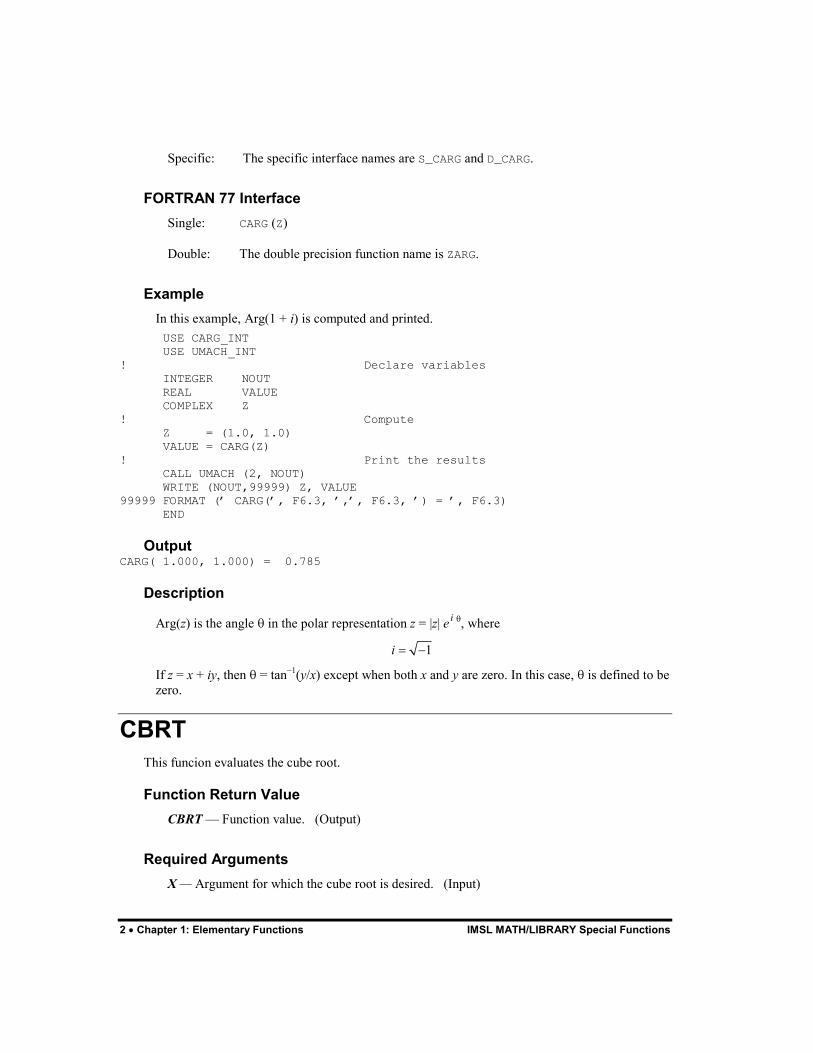
Example In this example, Arg(1 + i) is computed and printed.
USE CARG_INT USE UMACH_INT ! Declare variables INTEGER NOUT REAL VALUE COMPLEX Z ! Compute Z = (1.0, 1.0) VALUE = CARG(Z) ! Print the results CALL UMACH (2, NOUT) WRITE (NOUT,99999) Z, VALUE 99999 FORMAT (� CARG(�, F6.3, �,�, F6.3, �) = �, F6.3) END
Output CARG( 1.000, 1.000) = 0.785
Description
Arg(z) is the angle � in the polar representation z = |z| ei �, where
1i � �
If z = x + iy, then � = tan��(y/x) except when both x and y are zero. In this case, � is defined to be zero.
CBRT This funcion evaluates the cube root.
Function Return Value CBRT � Function value. (Output)
Required Arguments X � Argument for which the cube root is desired. (Input)
IMSL MATH/LIBRARY Special Functions Chapter 1: Elementary Functions � 3
FORTRAN 90 Interface Generic: CBRT (X)
Specific: The specific interface names are S_CBRT, D_CBRT, C_CBRT, AND Z_CBRT.
FORTRAN 77 Interface Single: CBRT (X)
Double: The double precision name is DCBRT.
Complex: The complex precision name is CCBRT.
Double Complex: The Double complex precision name is ZCBRT.
Example In this example, the cube root of 3.45 is computed and printed.
USE CBRT_INT USE UMACH_INT ! Declare variables INTEGER NOUT REAL VALUE, X ! Compute X = 3.45 VALUE = CBRT(X) ! Print the results CALL UMACH (2, NOUT) WRITE (NOUT,99999) X, VALUE 99999 FORMAT (� CBRT(�, F6.3, �) = �, F6.3) END
Output CBRT( 3.450) = 1.511
Comments For complex arguments, the branch cut for the cube root is taken along the negative real axis. The argument of the result, therefore, is greater than ��/3 and less than or equal to �/3. The other two roots are obtained by rotating the principal root by ��/3 and �/3.
Description The function CBRT(X) evaluates x���. All arguments are legal. For complex argument, x, the value of |x| must not overflow.
Additional Example In this example, the cube root of �3 + 0.0076i is computed and printed.
4 � Chapter 1: Elementary Functions IMSL MATH/LIBRARY Special Functions
USE UMACH_INT USE CBRT_INT ! Declare variables INTEGER NOUT COMPLEX VALUE, Z ! Compute Z = (-3.0, 0.0076) VALUE = CBRT(Z) ! Print the results CALL UMACH (2, NOUT) WRITE (NOUT,99999) Z, VALUE 99999 FORMAT (� CBRT((�, F7.4, �,�, F7.4, �)) = (�, & F6.3, �,�, F6.3, �)�) END
Output CBRT((-3.0000, 0.0076)) = ( 0.722, 1.248)
EXPRL This function evaluates the exponential function factored from first order, (EXP(X) � 1.0)/X.
Function Return Value EXPRL � Function value. (Output)
Required Arguments X � Argument for which the function value is desired. (Input)
FORTRAN 90 Interface Generic: EXPRL (X)
Specific: The specific interface names are S_EXPRL, D_EXPRL, and C_EXPRL.
FORTRAN 77 Interface Single: EXPRL (X)
Double: The double precision function name is DEXPRL.
Complex: The complex name is CEXPRL.
Example In this example, EXPRL(0.184) is computed and printed.
USE EXPRL_INT USE UMACH_INT
IMSL MATH/LIBRARY Special Functions Chapter 1: Elementary Functions � 5
! Declare variables INTEGER NOUT REAL VALUE, X ! Compute X = 0.184 VALUE = EXPRL(X) ! Print the results CALL UMACH (2, NOUT) WRITE (NOUT,99999) X, VALUE 99999 FORMAT (� EXPRL(�, F6.3, �) = �, F6.3) END
Output EXPRL( 0.184) = 1.098
Description
The function EXPRL(X) evaluates (ex � 1)/x. It will overflow if ex overflows. For complex arguments, z, the argument z must not be so close to a multiple of 2�i that substantial significance is lost due to cancellation. Also, the result must not overflow and |�z| must not be so large that the trigonometric functions are inaccurate.
Additional Example In this example, EXPRL(0.0076i) is computed and printed.
USE EXPRL_INT USE UMACH_INT ! Declare variables INTEGER NOUT COMPLEX VALUE, Z ! Compute Z = (0.0, 0.0076) VALUE = EXPRL(Z) ! Print the results CALL UMACH (2, NOUT) WRITE (NOUT,99999) Z, VALUE 99999 FORMAT (� EXPRL((�, F7.4, �,�, F7.4, �)) = (�, & F6.3, �,� F6.3, �)�) END
Output EXPRL(( 0.0000, 0.0076)) = ( 1.000, 0.004)
LOG10 This function extends FORTRAN�s generic log10 function to evauate the principal value of the complex common logarithm.
Function Return Value LOG10 � Complex function value. (Output)
6 � Chapter 1: Elementary Functions IMSL MATH/LIBRARY Special Functions
Required Arguments Z � Complex argument for which the function value is desired. (Input)
FORTRAN 90 Interface Generic: LOG10 (Z)
Specific: The specific interface names are CLOG10 and ZLOG10.
FORTRAN 77 Interface Complex: CLOG10 (Z)
Double complex: The double complex function name is ZLOG10.
Example In this example, the log��(0.0076i) is computed and printed.
USE LOG10_INT USE UMACH_INT
! Declare variables INTEGER NOUT COMPLEX VALUE, Z ! Compute Z = (0.0, 0.0076) VALUE = LOG10(Z) ! Print the results CALL UMACH (2, NOUT) WRITE (NOUT,99999) Z, VALUE 99999 FORMAT (� LOG10((�, F7.4, �,�, F7.4, �)) = (�, & F6.3, �,�, F6.3, �)�) END
Output LOG10(( 0.0000, 0.0076)) = (-2.119, 0.682)
Description The function LOG10(Z) evaluates log��(z) . The argument must not be zero, and |z| must not overflow.
ALNREL This function evaluates the natural logarithm of one plus the argument, or, in the case of complex argument, the principal value of the complex natural logarithm of one plus the argument.
IMSL MATH/LIBRARY Special Functions Chapter 1: Elementary Functions � 7
Function Return Value ALNREL � Function value. (Output)
Required Arguments X � Argument for the function. (Input)
FORTRAN 90 Interface Generic: ALNREL (X)
Specific: The specific interface names are S_ALNREL, D_ALNREL, and C_ALNREL.
FORTRAN 77 Interface Single: ALNREL (X)
Double: The double precision name function is DLNREL.
Complex: The comlpex name is CLNREL.
Example In this example, ln(1.189) = ALNREL(0.189) is computed and printed.
USE ALNREL_INT USE UMACH_INT ! Declare variables INTEGER NOUT REAL VALUE, X ! Compute X = 0.189 VALUE = ALNREL(X) ! Print the results CALL UMACH (2, NOUT) WRITE (NOUT,99999) X, VALUE 99999 FORMAT (� ALNREL(�, F6.3, �) = �, F6.3) END
Output ALNREL( 0.189) = 0.173
Comments 1. Informational error
Type Code
3 2 Result of ALNREL(X) is accurate to less than one-half precision because X is too near �1.0.

8 � Chapter 1: Elementary Functions IMSL MATH/LIBRARY Special Functions
2. ALNREL evaluates the natural logarithm of (1 + X) accurate in the sense of relative error even when X is very small. This routine (as opposed to the intrinsic ALOG) should be used to maintain relative accuracy whenever X is small and accurately known.
Description For real arguments, the function ALNREL(X) evaluates ln(1 + x) for x > �1. The argument x must be greater than �1.0 to avoid evaluating the logarithm of zero or a negative number. In addition, x must not be so close to �1.0 that considerable significance is lost in evaluating 1 + x.
For complex arguments, the function CLNREL(Z) evaluates ln(1 + z). The argument z must not be so close to �1 that considerable significance is lost in evaluating 1 + z. If it is, a recoverable error is issued; however, z = �1 is a fatal error because ln(1 + z) is infinite. Finally, |z| must not overflow.
Let = |z|, z = x + iy and r� = |1 + z|� = (1 + x)� + y� = 1 + 2x + �. Now, if is small, we may evaluate CLNREL(Z) accurately by
log(1 + z) = log r + iArg(z + 1)
= 1/2 log r� + iArg(z + 1)
= 1/2 ALNREL(2x + �) + iCARG(1 + z)
Additional Example In this example, ln(0.0076i) = ALNREL(�1 + 0.0076i) is computed and printed.
USE UMACH_INT USE ALNREL_INT ! Declare variables INTEGER NOUT COMPLEX VALUE, Z ! Compute Z = (-1.0, 0.0076) VALUE = ALNREL(Z) ! Print the results CALL UMACH (2, NOUT) WRITE (NOUT,99999) Z, VALUE 99999 FORMAT (� ALNREL((�, F8.4, �,�, F8.4, �)) = (�, & F8.4, �,�, F8.4, �)�) END
Output ALNREL((-1.000, .0076)) = (-4.880, 1.571)
IMSL MATH/LIBRARY Special Functions Chapter 2: Trigonometric and Hyperbolic Functions � 9
Chapter 2: Trigonometric and Hyperbolic Functions
Routines 2.1 Trigonometric Functions
Evaluates tan z for complex z...................................................TAN 10 Evaluates cot x for real x ......................................................... COT 11 Evaluates sin x for x a real angle in degrees........................SINDG 13 Evaluates cos x for x a real angle in degrees.....................COSDG 14 Evaluates sin�� z for complex z................................................ASIN 16 Evaluates cos�� z for complex z.............................................ACOS 17 Evaluates tan�� z for complex z ............................................. ATAN 18 Evaluates tan��(x/y) for x and y complex ............................. ATAN2 19
2.2 Hyperbolic Functions Evaluates sinh z for complex z ............................................... SINH 20 Evaluates cosh z for complex z .............................................COSH 21 Evaluates tanh z for complex z.............................................. TANH 23
2.3 Inverse Hyperbolic Functions Evaluates sinh�� x for real or complex x ...............................ASINH 24 Evaluates cosh�� x for real or complex x ............................ ACOSH 25 Evaluates tanh�� x for real or complex x ..............................ATANH 27
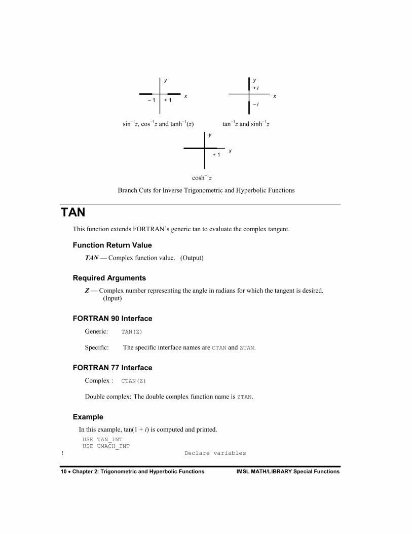
Usage Notes The complex inverse trigonometric hyperbolic functions are single-valued and regular in a slit complex plane. The branch cuts are shown below for z = x + iy, i.e., x = z and y = �z are the real and imaginary parts of z, respectively.
10 � Chapter 2: Trigonometric and Hyperbolic Functions IMSL MATH/LIBRARY Special Functions
� 1 + 1x
y
x
y+ i
� i
sin��z, cos��z and tanh��(z) tan��z and sinh��z
+ 1x
y
cosh��z
Branch Cuts for Inverse Trigonometric and Hyperbolic Functions
TAN This function extends FORTRAN�s generic tan to evaluate the complex tangent.
Function Return Value TAN � Complex function value. (Output)
Required Arguments Z � Complex number representing the angle in radians for which the tangent is desired.
(Input)
FORTRAN 90 Interface Generic: TAN(Z)
Specific: The specific interface names are CTAN and ZTAN.
FORTRAN 77 Interface Complex : CTAN(Z)
Double complex: The double complex function name is ZTAN.
Example In this example, tan(1 + i) is computed and printed.
USE TAN_INT USE UMACH_INT ! Declare variables
IMSL MATH/LIBRARY Special Functions Chapter 2: Trigonometric and Hyperbolic Functions � 11
INTEGER NOUT COMPLEX VALUE, Z ! Compute Z = (1.0, 1.0) VALUE = TAN(Z) ! Print the results CALL UMACH (2, NOUT) WRITE (NOUT,99999) Z, VALUE 99999 FORMAT (� TAN((�, F6.3, �,�, F6.3, �)) = (�, & F6.3, �,�, F6.3, �)�) END
Output TAN(( 1.000, 1.000)) = ( 0.272, 1.084)
Comments Informational error Type Code
3 2 Result of CTAN(Z) is accurate to less than one-half precision because the real part of Z is too near �/2 or 3�/2 when the imaginary part of Z is near zero or because the absolute value of the real part is very large and the absolute value of the imaginary part is small.
Description Let z = x + iy. If |cos z|� is very small, that is, if x is very close to �/2 or 3�/2 and if y is small, then tan z is nearly singular and a fatal error condition is reported. If |cos z|� is somewhat larger but still small, then the result will be less accurate than half precision. When 2x is so large that sin 2x cannot be evaluated to any nonzero precision, the following situation results. If |y| < 3/2, then CTAN cannot be evaluated accurately to better than one significant figure. If 3/2 � |y| < �1/2 ln �/2, then CTAN can be evaluated by ignoring the real part of the argument; however, the answer will be less accurate than half precision. Here, � = AMACH(4) is the machine precision.
COT This function evaluates the cotangent.
Function Value Return COT � Function value. (Output)
Required Arguments X � Angle in radians for which the cotangent is desired. (Input)
FORTRAN 90 Interface Generic: COT (X)
12 � Chapter 2: Trigonometric and Hyperbolic Functions IMSL MATH/LIBRARY Special Functions
Specific: The specific interface names are COT, DCOT, CCOT, and ZCOT.
FORTRAN 77 Interface Single: COT (X)
Double: The double precision function name is DCOT.
Complex: The complex name is CCOT.
Double Complex: The double complex name is ZCOT.
Example In this example, cot(0.3) is computed and printed.
USE COT_INT USE UMACH_INT ! Declare variables INTEGER NOUT REAL VALUE, X ! Compute X = 0.3 VALUE = COT(X) ! Print the results CALL UMACH (2, NOUT) WRITE (NOUT,99999) X, VALUE 99999 FORMAT (� COT(�, F6.3, �) = �, F6.3) END
Output COT( 0.300) = 3.233
Comments 1. Informational error for Real arguments:
Type Code
3 2 Result of COT(X) is accurate to less than one-half precision because ABS(X) is too large, or X is nearly a multiple of �.
Informational error for complex arguments Type Code
3 2 Result of CCOT(Z) is accurate to less than one-half precision because the real part of Z is too near a multiple of � when the imaginary part of Z is zero, or because the absolute value of the real part is very large and the absolute value of the imaginary part is small
2. Referencing COT(X) is NOT the same as computing 1.0/TAN(X) because the error conditions are quite different. For example, when X is near �/2, TAN(X) cannot be
IMSL MATH/LIBRARY Special Functions Chapter 2: Trigonometric and Hyperbolic Functions � 13
evaluated accurately and an error message must be issued. However, COT(X) can be evaluated accurately in the sense of absolute error.
Description For real x, the magnitude of x must not be so large that most of the computer word contains the integer part of x. Likewise, x must not be too near an integer multiple of �, although x close to the origin causes no accuracy loss. Finally, x must not be so close to the origin that COT(X) 1/x overflows.
For complex arguments, let z = x + iy. If |sin z|� is very small, that is, if x is very close to a multiple of � and if |y| is small, then cot z is nearly singular and a fatal error condition is reported. If |sin z|� is somewhat larger but still small, then the result will be less accurate than half precision. When |2x| is so large that sin 2x cannot be evaluated accurately to even zero precision, the following situation results. If |y| < 3/2, then CCOT cannot be evaluated accurately to be better than one significant figure. If 3/2 � |y| < �1/2 ln �/2, where � = AMACH(4) is the machine precision, then CCOT can be evaluated by ignoring the real part of the argument; however, the answer will be less accurate than half precision. Finally, |z| must not be so small that cot z 1/z overflows.
Additional Example In this example, cot(1 + i) is computed and printed.
USE COT_INT USE UMACH_INT
! Declare variables INTEGER NOUT COMPLEX VALUE, Z ! Compute Z = (1.0, 1.0) VALUE = COT(Z) ! Print the results CALL UMACH (2, NOUT) WRITE (NOUT,99999) Z, VALUE 99999 FORMAT (� COT((�, F6.3, �,�, F6.3, �)) = (�, & F6.3, �,�, F6.3, �)�) END
Output COT(( 1.000, 1.000)) = ( 0.218,-0.868)
SINDG This function evaluates the sine for the argument in degrees.
Function Return Value SINDG � Function value. (Output)
14 � Chapter 2: Trigonometric and Hyperbolic Functions IMSL MATH/LIBRARY Special Functions
Required Arguments X � Argument in degrees for which the sine is desired. (Input)
FORTRAN 90 Interface Generic: SINDG (X)
Specific: The specific interface names are S_SINDG and D_SINDG.
FORTRAN 77 Interface Single: SINDG (X)
Double: The double precision function name is DSINDG.
Example In this example, sin 45� is computed and printed.
USE SINDG_INT USE UMACH_INT
! Declare variables INTEGER NOUT REAL VALUE, X ! Compute X = 45.0 VALUE = SINDG(X) ! Print the results CALL UMACH (2, NOUT) WRITE (NOUT,99999) X, VALUE 99999 FORMAT (� SIN(�, F6.3, � deg) = �, F6.3) END
Output SIN(45.000 deg) = 0.707
Description To avoid unduly inaccurate results, the magnitude of x must not be so large that the integer part fills more than the computer word. Under no circumstances is the magnitude of x allowed to be larger than the largest representable integer because complete loss of accuracy occurs in this case.
COSDG This function evaluates the cosine for the argument in degrees.

IMSL MATH/LIBRARY Special Functions Chapter 2: Trigonometric and Hyperbolic Functions � 15
Function Return Value COSDG � Function value. (Output)
Required Arguments X � Argument in degrees for which the cosine is desired. (Input)
FORTRAN 90 Interface Generic: COSDG (X)
Specific: The specific interface names are S_COSDG and D_COSDG.
FORTRAN 77 Interface Single: COSDG (X)
Double: The double precision function name is DCOSDG.
Example In this example, cos 100� computed and printed.
USE COSDG_INT USE UMACH_INT
! Declare variables INTEGER NOUT REAL VALUE, X ! Compute X = 100.0 VALUE = COSDG(X) ! Print the results CALL UMACH (2, NOUT) WRITE (NOUT,99999) X, VALUE 99999 FORMAT (� COS(�, F6.2, � deg) = �, F6.3) END
Output COS(100.00 deg) = -0.174
Description To avoid unduly inaccurate results, the magnitude of x must not be so large that the integer part fills more than the computer word. Under no circumstances is the magnitude of x allowed to be larger than the largest representable integer because complete loss of accuracy occurs in this case.
16 � Chapter 2: Trigonometric and Hyperbolic Functions IMSL MATH/LIBRARY Special Functions
ASIN This function extends FORTRAN�s generic ASIN function to evaluate the complex arc sine.
Function Return Value ASIN � Complex function value in units of radians and the real part in the first or fourth
quadrant. (Output)
Required Arguments ZINP � Complex argument for which the arc sine is desired. (Input)
FORTRAN 90 Interface Generic: ASIN(ZINP)
Specific: The specific interface names are CASIN and ZASIN.
FORTRAN 77 Interface Complex: CASIN(ZINP)
Double complex: The double complex function name is ZASIN.
Example In this example, sin��(1 � i) is computed and printed.
USE ASIN_INT USE UMACH_INT ! Declare variables INTEGER NOUT COMPLEX VALUE, Z ! Compute Z = (1.0, -1.0) VALUE = ASIN(Z) ! Print the results CALL UMACH (2, NOUT) WRITE (NOUT,99999) Z, VALUE 99999 FORMAT (� ASIN((�, F6.3, �,�, F6.3, �)) = (�, & F6.3, �,�, F6.3, �)�) END
Output ASIN(( 1.000,-1.000)) = ( 0.666,-1.061)
IMSL MATH/LIBRARY Special Functions Chapter 2: Trigonometric and Hyperbolic Functions � 17
Description Almost all arguments are legal. Only when |z| > b/2 can an overflow occur. Here, b = AMACH(2) is the largest floating point number. This error is not detected by ASIN.
See Pennisi (1963, page 126) for reference.
ACOS This function extends FORTRAN�s generic ACOS function evaluate the complex arc cosine.
Function Return Value ACOS � Complex function value in units of radians with the real part in the first or second
quadrant. (Output)
Required Arguments Z � Complex argument for which the arc cosine is desired. (Input)
FORTRAN 90 Interface Generic: ACOS (Z)
Specific: The specific interface names are CACOS and ZACOS.
FORTRAN 77 Interface Complex: CACOS (Z)
Double complex: The double complex function name is ZACOS.
Example In this example, cos��(1 � i) is computed and printed.
USE ACOS_INT USE UMACH_INT
! Declare variables INTEGER NOUT COMPLEX VALUE, Z ! Compute Z = (1.0, -1.0) VALUE = ACOS(Z) ! Print the results CALL UMACH (2, NOUT) WRITE (NOUT,99999) Z, VALUE 99999 FORMAT (� ACOS((�, F6.3, �,�, F6.3, �)) = (�, & F6.3, �,�, F6.3, �)�) END

18 � Chapter 2: Trigonometric and Hyperbolic Functions IMSL MATH/LIBRARY Special Functions
Output ACOS(( 1.000,-1.000)) = ( 0.905, 1.061)
Description Almost all arguments are legal. Only when |z| > b/2 can an overflow occur. Here, b = AMACH(2) is the largest floating point number. This error is not detected by ACOS.
ATAN This function extends FORTRAN�s generic function ATAN to evaluate the complex arc tangent.
Function Return Value ATAN � Complex function value in units of radians with the real part in the first or fourth
quadrant. (Output)
Required Arguments Z � Complex argument for which the arc tangent is desired. (Input)
FORTRAN 90 Interface Generic: ATAN (Z)
Specific: The specific interface names are CATAN and ZATAN.
FORTRAN 77 Interface Complex: CATAN (Z)
Double complex: The double complex function name is ZATAN.
Example In this example, tan��(0.01 � 0.01i) is computed and printed.
USE ATAN_INT USE UMACH_INT
! Declare variables INTEGER NOUT COMPLEX VALUE, Z ! Compute Z = (0.01, 0.01) VALUE = ATAN(Z) ! Print the results CALL UMACH (2, NOUT) WRITE (NOUT,99999) Z, VALUE
IMSL MATH/LIBRARY Special Functions Chapter 2: Trigonometric and Hyperbolic Functions � 19
99999 FORMAT (� ATAN((�, F6.3, �,�, F6.3, �)) = (�, & F6.3, �,�, F6.3, �)�) END
Output ATAN(( 0.010, 0.010)) = ( 0.010, 0.010)
Comments Informational error
Type Code
3 2 Result of ATAN(Z) is accurate to less than one-half precision because |Z�| is too close to �1.0.
Description The argument z must not be exactly � i, because tan�� z is undefined there. In addition, z must not be so close to � i that substantial significance is lost.
ATAN2 This function extends FORTRAN�s generic function ATAN2 to evaluate the complex arc tangent of a ratio.
Function Return Value ATAN2 � Complex function value in units of radians with the real part between �� and �.
(Output)
Required Arguments CSN � Complex numerator of the ratio for which the arc tangent is desired. (Input)
CCS � Complex denominator of the ratio. (Input)
FORTRAN 90 Interface Generic: ATAN2(CSN, CCS)
Specific: The specific interface names are CATAN2 and ZATAN2.
FORTRAN 77 Interface Complex: CATAN2(CSN, CCS)
Double complex: The double complex function name is ZATAN2.
20 � Chapter 2: Trigonometric and Hyperbolic Functions IMSL MATH/LIBRARY Special Functions
Example In this example,
� � � �1 1/ 2 / 2tan
2i
i�
�
�
is computed and printed. USE ATAN2_INT USE UMACH_INT
! Declare variables INTEGER NOUT COMPLEX VALUE, X, Y ! Compute X = (2.0, 1.0) Y = (0.5, 0.5) VALUE = ATAN2(Y, X) ! Print the results CALL UMACH (2, NOUT) WRITE (NOUT,99999) Y, X, VALUE 99999 FORMAT (� ATAN2((�, F6.3, �,�, F6.3, �), (�, F6.3, �,�, F6.3,& �)) = (�, F6.3, �,�, F6.3, �)�) END
Output ATAN2(( 0.500, 0.500), ( 2.000, 1.000)) = ( 0.294, 0.092)
Comments The result is returned in the correct quadrant (modulo 2�).
Description Let z� = CSN and z� = CCS. The ratio z = z�/z� must not be � i because tan��(� i) is undefined. Likewise, z� and z� should not both be zero. Finally, z must not be so close to �i that substantial accuracy loss occurs.
SINH This function extends FORTRAN�s generic function SINH to evaluate the complex hyperbolic sine.
Function Return Value SINH � Complex function value. (Output)
Required Arguments Z � Complex number representing the angle in radians for which the complex hyperbolic
sine is desired. (Input)
IMSL MATH/LIBRARY Special Functions Chapter 2: Trigonometric and Hyperbolic Functions � 21
FORTRAN 90 Interface Generic: SINH(Z)
Specific: The specific interface names are CSINH and ZSINH.
FORTRAN 77 Interface Complex: CSINH(Z)
Double complex: The double complex function name is ZSINH.
Example In this example, sinh(5 � i) is computed and printed.
USE SINH_INT USE UMACH_INT ! Declare variables INTEGER NOUT COMPLEX VALUE, Z ! Compute Z = (5.0, -1.0) VALUE = SINH(Z) ! Print the results CALL UMACH (2, NOUT) WRITE (NOUT,99999) Z, VALUE 99999 FORMAT (� SINH((�, F6.3, �,�, F6.3, �)) = (�,& F7.3, �,�, F7.3, �)�) END
Output SINH(( 5.000,-1.000)) = ( 40.092,-62.446)
Description The argument z must satisfy
1/z �� �
where � = AMACH(4) is the machine precision and �z is the imaginary part of z.
COSH The function extends FORTRAN�s generic function COSH to evaluate the complex hyperbolic cosine.
Function Return Value COSH � Complex function value. (Output)
22 � Chapter 2: Trigonometric and Hyperbolic Functions IMSL MATH/LIBRARY Special Functions
Required Arguments Z � Complex number representing the angle in radians for which the hyperbolic cosine is
desired. (Input)
FORTRAN 90 Interface Generic: COSH (Z)
Specific: The specific interface names are CCOSH and ZCOSH.
FORTRAN 77 Interface Complex: CCOSH (Z)
Double complex: The double complex function name is ZCOSH.
Example In this example, cosh(�2 + 2i) is computed and printed.
USE COSH_INT USE UMACH_INT ! Declare variables INTEGER NOUT COMPLEX VALUE, Z ! Compute Z = (-2.0, 2.0) VALUE = COSH(Z) ! Print the results CALL UMACH (2, NOUT) WRITE (NOUT,99999) Z, VALUE 99999 FORMAT (� COSH((�, F6.3, �,�, F6.3, �)) = (�,& F6.3, �,�, F6.3, �)�) END
Output COSH((-2.000, 2.000)) = (-1.566,-3.298)
Description Let � = AMACH(4) be the machine precision. If |�z| is larger than
1/ �
then the result will be less than half precision, and a recoverable error condition is reported. If |�z| is larger than 1/�, the result has no precision and a fatal error is reported. Finally, if |z| is too large, the result overflows and a fatal error results. Here, z and �z represent the real and imaginary parts of z, respectively.
IMSL MATH/LIBRARY Special Functions Chapter 2: Trigonometric and Hyperbolic Functions � 23
TANH This function extends FORTRAN�s generic function TANH to evaluate the complex hyperbolic tangent.
Function Return Value TANH � Complex function value. (Output)
Required Arguments Z � Complex number representing the angle in radians for which the hyperbolic tangent is
desired. (Input)
FORTRAN 90 Interface Generic: TANH (Z)
Specific: The specific interface names are CTANH and ZTANH.
FORTRAN 77 Interface Complex: CTANH (Z)
Double complex: The double complex function name is ZTANH.
Example In this example, tanh(1 + i) is computed and printed.
USE TANH_INT USE UMACH_INT
! Declare variables INTEGER NOUT COMPLEX VALUE, Z ! Compute Z = (1.0, 1.0) VALUE = TANH(Z) ! Print the results CALL UMACH (2, NOUT) WRITE (NOUT,99999) Z, VALUE 99999 FORMAT (� TANH((�, F6.3, �,�, F6.3, �)) = (�,& F6.3, �,�, F6.3, �)�) END
Output TANH(( 1.000, 1.000)) = ( 1.084, 0.272)
24 � Chapter 2: Trigonometric and Hyperbolic Functions IMSL MATH/LIBRARY Special Functions
Description Let z = x + iy. If |cosh z|� is very small, that is, if y mod 2� is very close to �/2 or 3�/2 and if x is small, then tanh z is nearly singular; a fatal error condition is reported. If |cosh z|� is somewhat larger but still small, then the result will be less accurate than half precision. When 2y (z = x + iy) is so large that sin 2y cannot be evaluated accurately to even zero precision, the following situation results. If |x| < 3/2, then TANH cannot be evaluated accurately to better than one significant figure. If 3/2 � |y| < �1/2 ln (�/2), then TANH can be evaluated by ignoring the imaginary part of the argument; however, the answer will be less accurate than half precision. Here, � = AMACH(4) is the machine precision.
ASINH This function evaluates the arc hyperbolic sine.
Function Return Value ASINH � Function value. (Output)
Required Arguments X � Argument for which the arc hyperbolic sine is desired. (Input)
FORTRAN 90 Interface Generic: ASINH (X)
Specific: The specific interface names are ASINH, DASINH, CASINH, and ZASINH.
FORTRAN 77 Interface Single: ASINH (X)
Double: The double precision function name is DASINH.
Complex: The complex name is CASINH.
Double Complex: The double complex name is ZASINH
Example In this example, sinh��(2.0) is computed and printed.
USE ASINH_INT USE UMACH_INT ! Declare variables INTEGER NOUT REAL VALUE, X ! Compute
IMSL MATH/LIBRARY Special Functions Chapter 2: Trigonometric and Hyperbolic Functions � 25
X = 2.0 VALUE = ASINH(X) ! Print the results CALL UMACH (2, NOUT) WRITE (NOUT,99999) X, VALUE 99999 FORMAT (� ASINH(�, F6.3, �) = �, F6.3) END
Output ASINH( 2.000) = 1.444
Description The function ASINH(X) computes the inverse hyperbolic sine of x, sinh��x.
For complex arguments, almost all arguments are legal. Only when |z| > b/2 can an overflow occur, where b = AMACH(2) is the largest floating point number. This error is not detected by ASINH.
Additional Example In this example, sinh��(�1 + i) is computed and printed.
USE ASINH_INT USE UMACH_INT ! Declare variables INTEGER NOUT COMPLEX VALUE, Z ! Compute Z = (-1.0, 1.0) VALUE = ASINH(Z) ! Print the results CALL UMACH (2, NOUT) WRITE (NOUT,99999) Z, VALUE 99999 FORMAT (� ASINH((�, F6.3, �,�, F6.3, �)) = (�, & F6.3, �,�, F6.3, �)�) END
Output ASINH((-1.000, 1.000)) = (-1.061, 0.666)
ACOSH This function evaluates the arc hyperbolic cosine.
Function Return Value ACOSH � Function value. (Output)
Required Arguments X � Argument for which the arc hyperbolic cosine is desired. (Input)
26 � Chapter 2: Trigonometric and Hyperbolic Functions IMSL MATH/LIBRARY Special Functions
FORTRAN 90 Interface Generic: ACOSH (X)
Specific: The specific interface names are ACOSH, DACOSH, CACOSH, and ZACOSH.
FORTRAN 77 Interface Single: ACOSH (X)
Double: The double precision function name is DACOSH.
Complex: The complex name is CACOSH.
Double Complex: The double complex name is ZACOSH.
Example In this example, cosh��(1.4) is computed and printed.
USE ACOSH_INT USE UMACH_INT ! Declare variables INTEGER NOUT REAL VALUE, X ! Compute X = 1.4 VALUE = ACOSH(X) ! Print the results CALL UMACH (2, NOUT) WRITE (NOUT,99999) X, VALUE 99999 FORMAT (� ACOSH(�, F6.3, �) = �, F6.3) END
Output ACOSH( 1.400) = 0.867
Comments The result of ACOSH(X) is returned on the positive branch. Recall that, like SQRT(X), ACOSH(X) has multiple values.
Description The function ACOSH(X) computes the inverse hyperbolic cosine of x, cosh��x.
For complex arguments, almost all arguments are legal. Only when |z| > b/2 can an overflow occur, where b = AMACH(2) is the largest floating point number. This error is not detected by ACOSH.

IMSL MATH/LIBRARY Special Functions Chapter 2: Trigonometric and Hyperbolic Functions � 27
Additional Example In this example, cosh��(1 � i) is computed and printed.
USE ACOSH_INT USE UMACH_INT ! Declare variables INTEGER NOUT COMPLEX VALUE, Z ! Compute Z = (1.0, -1.0) VALUE = ACOSH(Z) ! Print the results CALL UMACH (2, NOUT) WRITE (NOUT,99999) Z, VALUE 99999 FORMAT (� ACOSH((�, F6.3, �,�, F6.3, �)) = (�, & F6.3, �,�, F6.3, �)�) END
Output ACOSH(( 1.000,-1.000)) = (-1.061, 0.905)
ATANH This function evaluates the arc hyperbolic tangent.
Function Return Value ATANH � Function value. (Output)
Required Arguments X � Argument for which the arc hyperbolic tangent is desired. (Input)
FORTRAN 90 Interface Generic: ATANH (X)
Specific: The specific interface names are ATANH, DATANH, CATANH, and ZATANH
FORTRAN 77 Interface Single: ATANH (X)
Double: The double precision function name is DATANH.
Complex: The complex name is CATANH.
Double Complex: The double complex name is ZATANH.
28 � Chapter 2: Trigonometric and Hyperbolic Functions IMSL MATH/LIBRARY Special Functions
Example In this example, tanh��(�1/4) is computed and printed.
USE ATANH_INT USE UMACH_INT ! Declare variables INTEGER NOUT REAL VALUE, X ! Compute X = -0.25 VALUE = ATANH(X) ! Print the results CALL UMACH (2, NOUT) WRITE (NOUT,99999) X, VALUE 99999 FORMAT (� ATANH(�, F6.3, �) = �, F6.3) END
Output ATANH(-0.250) = -0.255
Comments Informational error Type Code
3 2 Result of ATANH(X) is accurate to less than one-half precision because the absolute value of the argument is too close to 1.0.
Description ATANH(X) computes the inverse hyperbolic tangent of x, tanh��x. The argument x must satisfy
1x �� �
where � = AMACH(4) is the machine precision. Note that |x| must not be so close to one that the result is less accurate than half precision.
Additional Example In this example, tanh��(1/2 + i/2) is computed and printed.
USE ATANH_INT USE UMACH_INT ! Declare variables INTEGER NOUT COMPLEX VALUE, Z ! Compute Z = (0.5, 0.5) VALUE = ATANH(Z)

IMSL MATH/LIBRARY Special Functions Chapter 2: Trigonometric and Hyperbolic Functions � 29
! Print the results CALL UMACH (2, NOUT) WRITE (NOUT,99999) Z, VALUE 99999 FORMAT (� ATANH((�, F6.3, �,�, F6.3, �)) = (�, & F6.3, �,�, F6.3, �)�) END
Output
ATANH(( 0.500, 0.500)) = ( 0.402, 0.554)


IMSL MATH/LIBRARY Special Functions Chapter 3: Exponential Integrals and Related Functions � 31
Chapter 3: Exponential Integrals and Related Functions
Routines Evaluates the exponential integral, Ei(x) ......................................EI 32 Evaluates the exponential integral, E�(x).....................................E1 33 Evaluates the scaled exponential integrals, integer order, En(x) ..........................................................................................ENE 35 Evaluates the logarithmic integral, li(x) .......................................ALI 36 Evaluates the sine integral, Si(x) ..................................................SI 38 Evaluates the cosine integral, Ci(x) ............................................. CI 39 Evaluates the cosine integral (alternate definition)....................CIN 40 Evaluates the hyperbolic sine integral, Shi(x)............................SHI 42 Evaluates the hyperbolic cosine integral, Chi(x)........................CHI 43 Evaluates the hyperbolic cosine integral (alternate definition)CINH 44
Usage Notes The notation used in this chapter follows that of Abramowitz and Stegun (1964).
The following is a plot of the exponential integral functions that can be computed by the routines described in this chapter.

32 � Chapter 3: Exponential Integrals and Related Functions IMSL MATH/LIBRARY Special Functions
Figure 3-1 Plot of exE(x), E�(x) and Ei(x)
EI This function evaluates the exponential integral for arguments greater than zero and the Cauchy principal value for arguments less than zero.
Function Return Value EI � Function value. (Output)
Required Arguments X � Argument for which the function value is desired. (Input)
FORTRAN 90 Interface Generic: EI (X)
Specific: The specific interface names are S_EI and D_EI.
FORTRAN 77 Interface Single: EI (X)
IMSL MATH/LIBRARY Special Functions Chapter 3: Exponential Integrals and Related Functions � 33
Double: The double precision function name is DEI.
Example In this example, Ei(1.15) is computed and printed.
USE EI_INT USE UMACH_INT ! Declare variables INTEGER NOUT REAL VALUE, X ! Compute X = 1.15 VALUE = EI(X) ! Print the results CALL UMACH (2, NOUT) WRITE (NOUT,99999) X, VALUE 99999 FORMAT (� EI(�, F6.3, �) = �, F6.3) END
Output EI( 1.150) = 2.304
Comments If principal values are used everywhere, then for all X, EI(X) = �E1(�X) and E1(X) = �EI(�X)
Description The exponential integral, Ei(x), is defined to be
Ei( ) / for 0t
xx e t dt x
��
�
� � ��
The argument x must be large enough to insure that the asymptotic formula ex/x does not underflow, and x must not be so large that ex overflows.
E1 This function evaluates the exponential integral for arguments greater than zero and the Cauchy principal value of the integral for arguments less than zero.
Function Return Value E1 � Function value. (Output)
Required Arguments X � Argument for which the integral is to be evaluated. (Input)
34 � Chapter 3: Exponential Integrals and Related Functions IMSL MATH/LIBRARY Special Functions
FORTRAN 90 Interface Generic: E1 (X)
Specific: The specific interface names are S_E1 and D_E1.
FORTRAN 77 Interface Single: E1 (X)
Double: The double precision function name is DE1.
Example In this example, E�(1.3) is computed and printed.
USE E1_INT USE UMACH_INT ! Declare variables INTEGER NOUT REAL VALUE, X ! Compute X = 1.3 VALUE = E1(X) ! Print the results CALL UMACH (2, NOUT) WRITE (NOUT,99999) X, VALUE 99999 FORMAT (� E1(�, F6.3, �) = �, F6.3) END
Output E1( 1.300) = 0.135
Comments Informational error
Type Code
2 1 The function underflows because X is too large.
Description The alternate definition of the exponential integral, E�(x), is
1( ) / for 0t
xE x e t dt x
��
� ��
The path of integration must exclude the origin and not cross the negative real axis.
The argument x must be large enough that e�x does not overflow, and x must be small enough to insure that e�x/x does not underflow.
IMSL MATH/LIBRARY Special Functions Chapter 3: Exponential Integrals and Related Functions � 35
ENE Evaluates the exponential integral of integer order for arguments greater than zero scaled by EXP(X).
Required Arguments X � Argument for which the integral is to be evaluated. (Input)
It must be greater than zero.
N � Integer specifying the maximum order for which the exponential integral is to be calculated. (Input)
F � Vector of length N containing the computed exponential integrals scaled by EXP(X). (Output)
FORTRAN 90 Interface Generic: CALL ENE (X, N, F)
Specific: The specific interface names are S_ENE and D_ENE.
FORTRAN 77 Interface Single: CALL ENE (X, N, F)
Double: The double precision function name is DENE.
Example In this example, En(10) for n = 1, ..., n is computed and printed.
USE ENE_INT USE UMACH_INT
! Declare variables INTEGER N PARAMETER (N=10) ! INTEGER K, NOUT REAL F(N), X ! Compute X = 10.0 CALL ENE (X, N, F) ! Print the results CALL UMACH (2, NOUT) DO 10 K=1, N WRITE (NOUT,99999) K, X, F(K) 10 CONTINUE 99999 FORMAT (� E sub �, I2, � (�, F6.3, �) = �, F6.3) END
36 � Chapter 3: Exponential Integrals and Related Functions IMSL MATH/LIBRARY Special Functions
Output E sub 1 (10.000) = 0.092 E sub 2 (10.000) = 0.084 E sub 3 (10.000) = 0.078 E sub 4 (10.000) = 0.073 E sub 5 (10.000) = 0.068 E sub 6 (10.000) = 0.064 E sub 7 (10.000) = 0.060 E sub 8 (10.000) = 0.057 E sub 9 (10.000) = 0.054 E sub 10 (10.000) = 0.051
Description The scaled exponential integral of order n, En(x), is defined to be
1( ) for 0x xt n
nE x e e t dt x�
� �
� ��
The argument x must satisfy x > 0. The integer n must also be greater than zero. This code is based on a code due to Gautschi (1974).
ALI This function evaluates the logarithmic integral.
Function Return Value ALI � Function value. (Output)
Required Arguments X � Argument for which the logarithmic integral is desired. (Input)
It must be greater than zero and not equal to one.
FORTRAN 90 Interface Generic: ALI (X)
Specific: The specific interface names are S_ALI and D_ALI.
FORTRAN 77 Interface Single: ALI (X)
Double: The double precision function name is DALI.

IMSL MATH/LIBRARY Special Functions Chapter 3: Exponential Integrals and Related Functions � 37
Example In this example, li(2.3) is computed and printed.
USE ALI_INT USE UMACH_INT
! Declare variables INTEGER NOUT REAL VALUE, X ! Compute X = 2.3 VALUE = ALI(X) ! Print the results CALL UMACH (2, NOUT) WRITE (NOUT,99999) X, VALUE 99999 FORMAT (� ALI(�, F6.3, �) = �, F6.3) END
Output ALI( 2.300) = 1.439
Comments Informational error
Type Code
3 2 Result of ALI(X) is accurate to less than one-half precision because X is too close to 1.0.
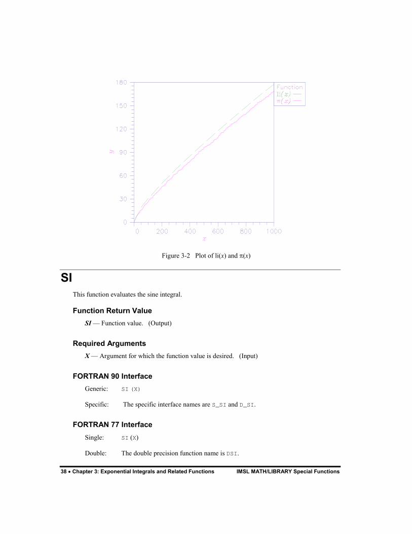
Description The logarithmic integral, li(x), is defined to be
0li( ) for 0 and 1
lnx dtx x x
t� � � ��
The argument x must be greater than zero and not equal to one. To avoid an undue loss of accuracy, x must be different from one at least by the square root of the machine precision.
The function li(x) approximates the function �(x), the number of primes less than or equal to x. Assuming the Riemann hypothesis (all non-real zeros of �(z) are on the line z = 1/2), then
li( ) ( ) ( ln )x x O x x� � �
38 � Chapter 3: Exponential Integrals and Related Functions IMSL MATH/LIBRARY Special Functions
Figure 3-2 Plot of li(x) and �(x)
SI This function evaluates the sine integral.
Function Return Value SI � Function value. (Output)
Required Arguments X � Argument for which the function value is desired. (Input)
FORTRAN 90 Interface Generic: SI (X)
Specific: The specific interface names are S_SI and D_SI.
FORTRAN 77 Interface Single: SI (X)
Double: The double precision function name is DSI.
IMSL MATH/LIBRARY Special Functions Chapter 3: Exponential Integrals and Related Functions � 39
Example In this example, Si(1.25) is computed and printed.
USE SI_INT USE UMACH_INT ! Declare variables INTEGER NOUT REAL VALUE, X ! Compute X = 1.25 VALUE = SI(X) ! Print the results CALL UMACH (2, NOUT) WRITE (NOUT,99999) X, VALUE 99999 FORMAT (� SI(�, F6.3, �) = �, F6.3) END
Output SI( 1.250) = 1.146
Description The sine integral, Si(x), is defined to be
0sinSi( )=
x tx dtt�
If
1/x ��
the answer is less accurate than half precision, while for |x| > 1 /�, the answer has no precision. Here, � = AMACH(4) is the machine precision.
CI This function evaluates the cosine integral.
Function Return Value CI � Function value. (Output)
Required Arguments X � Argument for which the function value is desired. (Input)
It must be greater than zero.
40 � Chapter 3: Exponential Integrals and Related Functions IMSL MATH/LIBRARY Special Functions
FORTRAN 90 Interface Generic: CI (X)
Specific: The specific interface names are S_CI and D_CI.
FORTRAN 77 Interface Single: CI (X)
Double: The double precision function name is DCI.
Example In this example, Ci(1.5) is computed and printed.
USE CI_INT USE UMACH_INT ! Declare variables INTEGER NOUT REAL VALUE, X ! Compute X = 1.5 VALUE = CI(X) ! Print the results CALL UMACH (2, NOUT) WRITE (NOUT,99999) X, VALUE 99999 FORMAT (� CI(�, F6.3, �) = �, F6.3) END
Output CI( 1.500) = 0.470
Description The cosine integral, Ci(x), is defined to be
0
1 cosCi( ) lnx
ttx x d
t�
�
� � � �
where � 0.57721566 is Euler�s constant.
The argument x must be larger than zero. If
1/x ��
then the result will be less accurate than half precision. If x > 1/�, the result will have no precision. Here, � = AMACH(4) is the machine precision.
CIN This function evaluates a function closely related to the cosine integral.
IMSL MATH/LIBRARY Special Functions Chapter 3: Exponential Integrals and Related Functions � 41
Function Return Value CIN � Function value. (Output)
Required Arguments X � Argument for which the function value is desired. (Input)
FORTRAN 90 Interface Generic: CIN (X)
Specific: The specific interface names are S_CIN and D_CIN.
FORTRAN 77 Interface Single: CIN (X)
Double: The double precision function name is DCIN.
Example In this example, Cin(2�) is computed and printed.
USE CIN_INT USE UMACH_INT USE CONST_INT ! Declare variables ! INTEGER NOUT REAL VALUE, X ! Compute X = CONST(�pi�) X = 2.0* X VALUE = CIN(X) ! Print the results CALL UMACH (2, NOUT) WRITE (NOUT,99999) X, VALUE 99999 FORMAT (� CIN(�, F6.3, �) = �, F6.3) END
Output CIN( 6.283) = 2.438
Comments Informational error Type Code
2 1 The function underflows because X is too small.
42 � Chapter 3: Exponential Integrals and Related Functions IMSL MATH/LIBRARY Special Functions
Description The alternate definition of the cosine integral, Cin(x), is
0
1 cosCin( )x tx dt
t�
� �
For
0 x s� �
where s = AMACH(1) is the smallest representable positive number, the result underflows. For
1/x ��
the answer is less accurate than half precision, while for |x| > 1 /�, the answer has no precision. Here, � = AMACH(4) is the machine precision.
SHI This function evaluates the hyperbolic sine integral.
Function Return Value SHI� function value. (Output)
SHI equals
0sinh( ) /
xt t dt�
Required Arguments X � Argument for which the function value is desired. (Input)
FORTRAN 90 Interface Generic: SHI (X)
Specific: The specific interface names are S_SHI and D_SHI.
FORTRAN 77 Interface Single: SHI (X)
Double: The double precision function name is DSHI.
Example In this example, Shi(3.5) is computed and printed.
IMSL MATH/LIBRARY Special Functions Chapter 3: Exponential Integrals and Related Functions � 43
USE SHI_INT USE UMACH_INT ! Declare variables INTEGER NOUT REAL VALUE, X ! Compute X = 3.5 VALUE = SHI(X) ! Print the results CALL UMACH (2, NOUT) WRITE (NOUT,99999) X, VALUE 99999 FORMAT (� SHI(�, F6.3, �) = �, F6.3) END
Output SHI( 3.500) = 6.966
Description The hyperbolic sine integral, Shi(x), is defined to be
0
sinhShi( )x tx dt
t� �
The argument x must be large enough that e�x/x does not underflow, and x must be small enough that ex does not overflow.
CHI This function evaluates the hyperbolic cosine integral.
Function Return Value CHI � Function value. (Output)
Required Arguments X � Argument for which the function value is desired. (Input)
FORTRAN 90 Interface Generic: CHI (X)
Specific: The specific interface names are S_CHI and D_CHI.
FORTRAN 77 Interface Single: CHI (X)
44 � Chapter 3: Exponential Integrals and Related Functions IMSL MATH/LIBRARY Special Functions
Double: The double precision function name is DCHI.
Example In this example, Chi(2.5) is computed and printed.
USE CHI_INT USE UMACH_INT
! Declare variables INTEGER NOUT REAL VALUE, X ! Compute X = 2.5 VALUE = CHI(X) ! Print the results CALL UMACH (2, NOUT) WRITE (NOUT,99999) X, VALUE 99999 FORMAT (� CHI(�, F6.3, �) = �, F6.3) END
Output CHI( 2.500) = 3.524
Comments When X is negative, the principal value is used.
Description The hyperbolic cosine integral, Chi(x), is defined to be
0
cosh 1Chi( ) ln for 0x tx x dt x
t�
�
� � � ��
where � 0.57721566 is Euler�s constant.
The argument x must be large enough that e�x/x does not underflow, and x must be small enough that ex does not overflow.
CINH This function evaluates a function closely related to the hyperbolic cosine integral.
Function Return Value CINH � Function value. (Output)
Required Arguments X � Argument for which the function value is desired. (Input)
IMSL MATH/LIBRARY Special Functions Chapter 3: Exponential Integrals and Related Functions � 45
FORTRAN 90 Interface Generic: CINH (X)
Specific: The specific interface names are S_CINH and D_CINH.
FORTRAN 77 Interface Single: CINH (X)
Double: The double precision function name is DCINH.
Example In this example, Cinh(2.5) is computed and printed.
USE CINH_INT USE UMACH_INT
! Declare variables INTEGER NOUT REAL VALUE, X ! Compute X = 2.5 VALUE = CINH(X) ! Print the results CALL UMACH (2, NOUT) WRITE (NOUT,99999) X, VALUE 99999 FORMAT (� CINH(�, F6.3, �) = �, F6.3) END
Output
CINH( 2.500) = 2.031
Comments Informational error Type Code
2 1 The function underflows because X is too small.
Description The alternate definition of the hyperbolic cosine integral, Cinh(x), is
0
cosh 1Cinh( )x tx dt
t�
� �
For
0 2x s� �

46 � Chapter 3: Exponential Integrals and Related Functions IMSL MATH/LIBRARY Special Functions
where s = AMACH(1) is the smallest representable positive number, the result underflows. The argument x must be large enough that e�x/x does not underflow, and x must be small enough that ex does not overflow.
IMSL MATH/LIBRARY Special Functions Chapter 4: Gamma Function and Related Functions � 47
Chapter 4: Gamma Function and Related Functions
Routines 4.1 Factorial Function
Evaluates the factorial, n� .........................................................FAC 48
Evaluates the binomial coefficient, nm
� �� �� �� �
................................ BINOM 50
4.2 Gamma Function Evaluates the real or complex gamma function, �(x) ........ GAMMA 51 Evaluates the reciprocal of the real or complex gamma function, 1/�(x) ...................................................................... GAMR 54 Evaluates the real or complex function, ln ��(x)�................ALNGAM 55 Evaluates the log abs gamma function and its sign .........ALGAMS 57
4.3. Incomplete Gamma Function Evaluates the incomplete gamma function, �(a,x) ..................GAMI 59 Evaluates the complementary incomplete gamma function, �(a,x).................................................................................... GAMIC 61 Evaluates Tricomi�s incomplete gamma function, �*(a, x) ....GAMIT 63
4.4. Psi Function Evaluates the real or complex psi function, �(x) ....................... PSI 64
4.5. Pochhammer�s Function Evaluates Pochhammer�s generalized symbol, (a)x ..............POCH 66 Evaluates Pochhammer�s symbol starting from the first order ...............................................................POCH1 67
4.6. Beta Function Evaluates the real or complex beta function, �(a,b) ...............BETA 69 Evaluates the log of the real or complex beta function, ln �(a,b).............................................................................. ALBETA 71 Evaluates the incomplete beta function, Ix(a,b) .....................BETAI 73
48 � Chapter 4: Gamma Function and Related Functions IMSL MATH/LIBRARY Special Functions
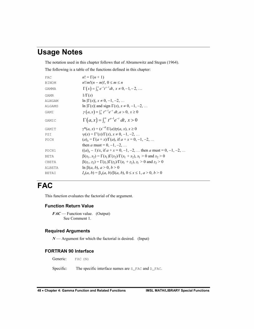
Usage Notes The notation used in this chapter follows that of Abramowitz and Stegun (1964).
The following is a table of the functions defined in this chapter:
FAC n! = �(n + 1) BINOM n!/m!(n � m)!, 0 � m � n GAMMA � � 1
0 , 0, 1, 2,t xx e t dt x� � �� � � � �� �
GAMR 1/�(x) ALNGAM ln ��(x)�, x � 0, �1, �2, � ALGAMS ln ��(x)� and sign �(x), x � 0, �1, �2, � GAMI � � 1
0, , 0, 0x a ta x t e dt a x�� �� � ��
GAMIC � � 1, , 0a txa x t e dt x� � �� � ��
GAMIT �*(a, x) = (x�a/�(a))�(a, x), x � 0 PSI �(x) = ��(x)/�(x), x � 0, �1, �2, � POCH (a)x = �(a + x)/�(a), if a + x = 0, �1, �2, � then a must = 0, �1, �2, � POCH1 ((a)x � 1)/x, if a + x = 0, �1, �2, � then a must = 0, �1, �2, � BETA �(x�, x�) = �(x�)�(x�)/�(x� + x�), x� > 0 and x� > 0 CBETA �(z�, z�) = �(z�)�(z�)/�(z� + z�), z� > 0 and z� > 0 ALBETA ln �(a, b), a > 0, b > 0 BETAI Ix(a, b) = �x(a, b)/�(a, b), 0 � x � 1, a > 0, b > 0
FAC This function evaluates the factorial of the argument.
Function Return Value FAC � Function value. (Output)
See Comment 1.
Required Arguments N � Argument for which the factorial is desired. (Input)
FORTRAN 90 Interface Generic: FAC (N)
Specific: The specific interface names are S_FAC and D_FAC.
IMSL MATH/LIBRARY Special Functions Chapter 4: Gamma Function and Related Functions � 49
FORTRAN 77 Interface Single: FAC (N)
Double: The double precision function name is DFAC.
Example In this example, 6! is computed and printed.
USE FAC_INT USE UMACH_INT ! Declare variables INTEGER N, NOUT REAL VALUE ! Compute N = 6 VALUE = FAC(N) ! Print the results CALL UMACH (2, NOUT) WRITE (NOUT,99999) N, VALUE 99999 FORMAT (� FAC(�, I1, �) = �, F6.2) END
Output FAC(6) = 720.00
Comments 1. If the generic version of this function is used, the immediate result must be stored in a
variable before use in an expression. For example:
X = FAC(6) Y = SQRT(X) must be used rather than
Y = SQRT(FAC(6)).
If this is too much of a restriction on the programmer, then the specific name can be used without this restriction.
To evaluate the factorial for nonintegral values of the argument, the gamma function should be used. For large values of the argument, the log gamma function should be used.
Description The factorial is computed using the relation n! = �(n + 1). The function �(x) is defined in GAMMA on page 51. The argument n must be greater than or equal to zero, and it must not be so large that n! overflows. Approximately, n! overflows when nne�n overflows.
50 � Chapter 4: Gamma Function and Related Functions IMSL MATH/LIBRARY Special Functions
BINOM This function evaluates the binomial coefficient.
Function Return Value BINOM � Function value. (Output)
See Comment 1.
Required Arguments N � First parameter of the binomial coefficient. (Input)
N must be nonnegative.
M � Second parameter of the binomial coefficient. (Input) M must be nonnegative and less than or equal to N.
FORTRAN 90 Interface Generic: BINOM (N, M)
Specific: The specific interface names are S_BINOM and D_BINOM.
FORTRAN 77 Interface Single: BINOM (N, M)
Double: The double precision function name is DBINOM.
Example
In this example, 95� �� �� �
is computed and printed.
USE BINOM_INT USE UMACH_INT ! Declare variables INTEGER M, N, NOUT REAL VALUE ! Compute N = 9 M = 5 VALUE = BINOM(N, M) ! Print the results CALL UMACH (2, NOUT) WRITE (NOUT,99999) N, M, VALUE 99999 FORMAT (� BINOM(�, I1, �,�, I1, �) = �, F6.2) END
IMSL MATH/LIBRARY Special Functions Chapter 4: Gamma Function and Related Functions � 51
Output BINOM(9,5) = 126.00
Comments 1. If the generic version of this function is used, the immediate result must be stored in a
variable before use in an expression. For example:
X = BINOM(9, 5) Y = SQRT(X) must be used rather than
Y = SQRT(BINOM(9, 5)).
If this is too much of a restriction on the programmer, then the specific name can be used without this restriction.
2. To evaluate binomial coefficients for nonintegral values of the arguments, the complete beta function or log beta function should be used.
Description The binomial function is defined to be
!!( )!
n nm m n m
� ��� �
�� �
with n � m � 0. Also, n must not be so large that the function overflows.
GAMMA This function evaluates the complete gamma function.
Function Return Value GAMMA � Function value. (Output)
Required Arguments X � Argument for which the complete gamma function is desired. (Input)
FORTRAN 90 Interface Generic: GAMMA (X)
Specific: The specific interface names are S_GAMMA, D_GAMMA, and C_GAMMA.

52 � Chapter 4: Gamma Function and Related Functions IMSL MATH/LIBRARY Special Functions
FORTRAN 77 Interface Single: GAMMA (X)
Double: The double precision function name is DGAMMA.
Complex: The complex name is CGAMMA.
Example In this example, �(5.0) is computed and printed.
USE GAMMA_INT USE UMACH_INT ! Declare variables INTEGER NOUT REAL VALUE, X ! Compute X = 5.0 VALUE = GAMMA(X) ! Print the results CALL UMACH (2, NOUT) WRITE (NOUT,99999) X, VALUE 99999 FORMAT (� GAMMA(�, F6.3, �) = �, F6.3) END
Output GAMMA( 5.000) = 24.000
Comments Informational errors Type Code
2 1 The function underflows because X is too small.
3 2 Result is accurate to less than one-half precision because X is too near a negative integer.
Description The gamma function, �(z), is defined to be
� � 1
0 for 0z tz t e dt z
�� �
� � � ��
For (z) < 0, the above definition is extended by analytic continuation.
z must not be so close to a negative integer that the result is less accurate than half precision. If (z) is too small, then the result will underflow. Users who need such values should use the log gamma function ALNGAM, page 55. When �(z) 0, (z) should be greater than x� so that the
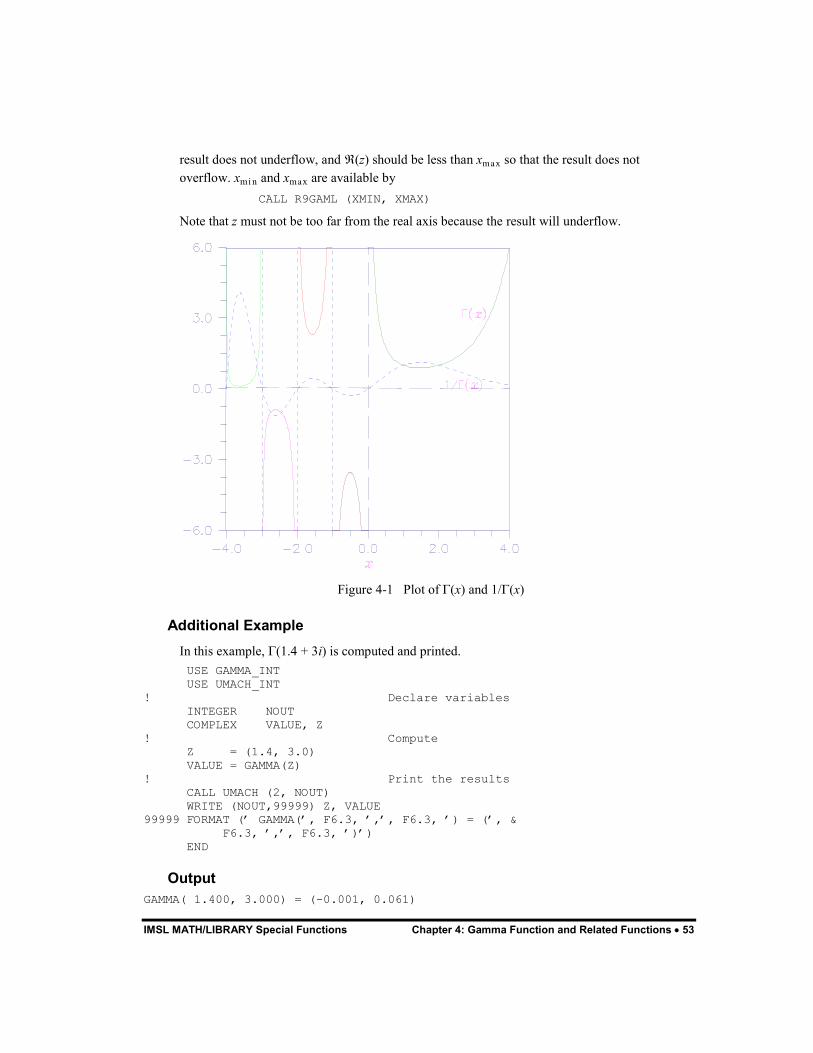
IMSL MATH/LIBRARY Special Functions Chapter 4: Gamma Function and Related Functions � 53
result does not underflow, and (z) should be less than x� so that the result does not overflow. x� and x� are available by
CALL R9GAML (XMIN, XMAX)
Note that z must not be too far from the real axis because the result will underflow.
Figure 4-1 Plot of �(x) and 1/�(x)
Additional Example In this example, �(1.4 + 3i) is computed and printed.
USE GAMMA_INT USE UMACH_INT ! Declare variables INTEGER NOUT COMPLEX VALUE, Z ! Compute Z = (1.4, 3.0) VALUE = GAMMA(Z) ! Print the results CALL UMACH (2, NOUT) WRITE (NOUT,99999) Z, VALUE 99999 FORMAT (� GAMMA(�, F6.3, �,�, F6.3, �) = (�, & F6.3, �,�, F6.3, �)�) END
Output GAMMA( 1.400, 3.000) = (-0.001, 0.061)
54 � Chapter 4: Gamma Function and Related Functions IMSL MATH/LIBRARY Special Functions
GAMR This function evaluates the reciprocal gamma function.
Function Return Value GAMR � Function value. (Output)
Required Arguments X � Argument for which the reciprocal gamma function is desired. (Input)
FORTRAN 90 Interface Generic: GAMR (X)
Specific: The specific interface names are S_GAMR, D_GAMR, and C_GAMR
FORTRAN 77 Interface Single: GAMR (X)
Double: The double precision function name is DGAMR.
Complex: The complex name is CGAMR.
Example In this example, 1/�(1.85) is computed and printed.
USE GAMR_INT USE UMACH_INT
! Declare variables INTEGER NOUT REAL VALUE, X ! Compute X = 1.85 VALUE = GAMR(X) ! Print the results CALL UMACH (2, NOUT) WRITE (NOUT,99999) X, VALUE 99999 FORMAT (� GAMR(�, F6.3, �) = �, F6.3) END
Output GAMR( 1.850) = 1.058
Comments This function is well behaved near zero and negative integers.
IMSL MATH/LIBRARY Special Functions Chapter 4: Gamma Function and Related Functions � 55
Description The function GAMR computes 1/�(z). See GAMMA (page 51) for the definition of �(z).
For �(z) 0, z must be larger than x� so that 1/�(z) does not underflow, and x must be smaller than x� so that 1/��z) does not overflow. Symmetric overflow and underflow limits x� and x� are obtainable from
CALL R9GAML (XMIN, XMAX)
Note that z must not be too far from the real axis because the result will overflow there.
Additional Example In this example, ln ��1.4 + 3i) is computed and printed.
USE GAMR_INT USE UMACH_INT
! Declare variables INTEGER NOUT COMPLEX VALUE, Z ! Compute Z = (1.4, 3.0) VALUE = GAMR(Z) ! Print the results CALL UMACH (2, NOUT) WRITE (NOUT,99999) Z, VALUE 99999 FORMAT (� GAMR(�, F6.3, �,�, F6.3, �) = (�, F7.3, �,�, F7.3, �)�) END
Output GAMR( 1.400, 3.000) = ( -0.303,-16.367)
ALNGAM The function evaluates the logarithm of the absolute value of the gamma function.
Function Return Value ALNGAM � Function value. (Output)
Required Arguments X � Argument for which the function value is desired. (Input)
FORTRAN 90 Interface Generic: ALNGAM (X)
Specific: The specific interface names are S_ALNGAM, D_ALNGAM, and C_ALNGAM.

56 � Chapter 4: Gamma Function and Related Functions IMSL MATH/LIBRARY Special Functions
FORTRAN 77 Interface Single: ALNGAM (X)
Double: The double precision function name is DLNGAM.
Complex: The complex name is CLNGAM.
Example In this example, ln ���1.85)� is computed and printed.
USE ALNGAM_INT USE UMACH_INT ! Declare variables INTEGER NOUT REAL VALUE, X ! Compute X = 1.85 VALUE = ALNGAM(X) ! Print the results CALL UMACH (2, NOUT) WRITE (NOUT,99999) X, VALUE 99999 FORMAT (� ALNGAM(�, F6.3, �) = �, F6.3) END
Output ALNGAM( 1.850) = -0.056
Comments Informational error Type Code
3 2 Result of ALNGAM(X) is accurate to less than one-half precision because X is too near a negative integer.
Description The function ALNGAM computes ln ���x)�. See GAMMA (page 51) for the definition of ��x).
The gamma function is not defined for integers less than or equal to zero. Also, |x| must not be so large that the result overflows. Neither should x be so close to a negative integer that the accuracy is worse than half precision.

IMSL MATH/LIBRARY Special Functions Chapter 4: Gamma Function and Related Functions � 57
Figure 4-2 Plot of log���x)�
Additional Example In this example, ln ��1.4 + 3i) is computed and printed.
USE ALNGAM_INT USE UMACH_INT ! Declare variables INTEGER NOUT COMPLEX VALUE, Z ! Compute Z = (1.4, 3.0) VALUE = ALNGAM(Z) ! Print the results CALL UMACH (2, NOUT) WRITE (NOUT,99999) Z, VALUE 99999 FORMAT (� ALNGAM(�, F6.3, �,�, F6.3, �) = (�,& F6.3, �,�, F6.3, �)�) END
Output ALNGAM( 1.400, 3.000) = (-2.795, 1.589)
ALGAMS Returns the logarithm of the absolute value of the gamma function and the sign of gamma.

58 � Chapter 4: Gamma Function and Related Functions IMSL MATH/LIBRARY Special Functions
Required Arguments X � Argument for which the logarithm of the absolute value of the gamma function is
desired. (Input)
ALGM � Result of the calculation. (Output)
S � Sign of gamma(X). (Output) If gamma(X) is greater than or equal to zero, S = 1.0. If gamma(X) is less than zero, S = �1.0.
FORTRAN 90 Interface Generic: CALL ALGAMS (X, ALGM, S)
Specific: The specific interface names are S_ALGAMS and D_ALGAMS.
FORTRAN 77 Interface Single: CALL ALGAMS (X, ALGM, S)
Double: The double precision function name is DLGAMS.
Example In this example, ln ���1.85)� and the sign of ��1.85) are computed and printed.
USE ALGAMS_INT USE UMACH_INT ! Declare variables INTEGER NOUT REAL VALUE, S, X ! Compute X = 1.85 CALL ALGAMS(X, VALUE, S) ! Print the results CALL UMACH (2, NOUT) WRITE (NOUT,99998) X, VALUE 99998 FORMAT (� Log Abs(Gamma(�, F6.3, �)) = �, F6.3) WRITE (NOUT,99999) X, S 99999 FORMAT (� Sign(Gamma(�, F6.3, �)) = �, F6.2) END
Output Log Abs(Gamma( 1.850)) = -0.056 Sign(Gamma( 1.850)) = 1.00
IMSL MATH/LIBRARY Special Functions Chapter 4: Gamma Function and Related Functions � 59
Comments Informational error Type Code
3 2 Result of ALGAMS is accurate to less than one-half precision because X is too near a negative integer.
Description The function ALGAMS computes ln ���x)� and the sign of ��x). See GAMMA (page 51) for the definition of ��x).
The result overflows if |x| is too large. The accuracy is worse than half precision if x is too close to a negative integer.
GAMI This funciton evaluates the incomplete gamma function.
Function Return Value GAMI � Function value. (Output)
Required Arguments A � The integrand exponent parameter. (Input)
It must be positive.
X � The upper limit of the integral definition of GAMI. (Input) It must be nonnegative.
FORTRAN 90 Interface Generic: GAMI(A, X)
Specific: The specific interface names are S_GAMI and D_GAMI.
FORTRAN 77 Interface Single: GAMI(A, X)
Double: The double precision function name is DGAMI.
Example In this example, �(2.5, 0.9) is computed and printed.
60 � Chapter 4: Gamma Function and Related Functions IMSL MATH/LIBRARY Special Functions
USE GAMI_INT USE UMACH_INT ! Declare variables INTEGER NOUT REAL A, VALUE, X ! Compute A = 2.5 X = 0.9 VALUE = GAMI(A, X) ! Print the results CALL UMACH (2, NOUT) WRITE (NOUT,99999) A, X, VALUE 99999 FORMAT (� GAMI(�, F6.3, �,�, F6.3, �) = �, F6.4) END
Output GAMI( 2.500, 0.900) = 0.1647
Description The incomplete gamma function is defined to be
� � 1
0, for 0 and 0
x a ta x t e dt a x�� �
� � ��
The function �(a, x) is defined only for a greater than zero. Although �(a, x) is well defined for x > ��, this algorithm does not calculate �(a, x) for negative x. For large a and sufficiently large x, �(a, x) may overflow. �(a, x) is bounded by ��a), and users may find this bound a useful guide in determining legal values of a.
Because logarithmic variables are used, a slight deterioration of two or three digits of accuracy will occur when GAMI is very large or very small.
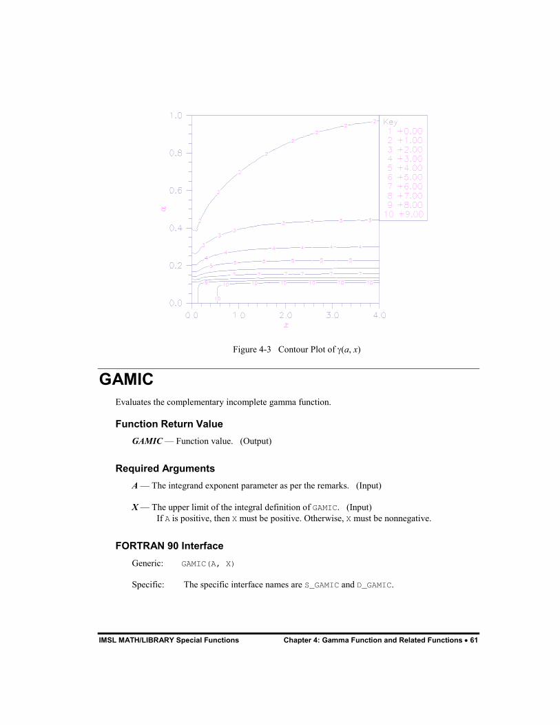
IMSL MATH/LIBRARY Special Functions Chapter 4: Gamma Function and Related Functions � 61
Figure 4-3 Contour Plot of �(a, x)
GAMIC Evaluates the complementary incomplete gamma function.
Function Return Value GAMIC � Function value. (Output)
Required Arguments A � The integrand exponent parameter as per the remarks. (Input)
X � The upper limit of the integral definition of GAMIC. (Input) If A is positive, then X must be positive. Otherwise, X must be nonnegative.
FORTRAN 90 Interface Generic: GAMIC(A, X)
Specific: The specific interface names are S_GAMIC and D_GAMIC.
62 � Chapter 4: Gamma Function and Related Functions IMSL MATH/LIBRARY Special Functions
FORTRAN 77 Interface Single: GAMIC(A, X)
Double: The double precision function name is DGAMIC.
Example In this example, ��2.5, 0.9) is computed and printed.
USE GAMIC_INT USE UMACH_INT ! Declare variables INTEGER NOUT REAL A, VALUE, X ! Compute A = 2.5 X = 0.9 VALUE = GAMIC(A, X) ! Print the results CALL UMACH (2, NOUT) WRITE (NOUT,99999) A, X, VALUE 99999 FORMAT (� GAMIC(�, F6.3, �,�, F6.3, �) = �, F6.4) END
Output GAMIC( 2.500, 0.900) = 1.1646
Comments Informational error Type Code
3 2 Result of GAMIC(A, X) is accurate to less than one-half precision because A is too near a negative integer.
Description The incomplete gamma function is defined to be
� � 1, a t
xa x t e dt
�� �
� � �
The only general restrictions on a are that it must be positive if x is zero; otherwise, it must not be too close to a negative integer such that the accuracy of the result is less than half precision. Furthermore, ��a, x) must not be so small that it underflows, or so large that it overflows. Although ��a, x) is well defined for x > �� and a > 0, this algorithm does not calculate ��a, x) for negative x.
The function GAMIC is based on a code by Gautschi (1979).
IMSL MATH/LIBRARY Special Functions Chapter 4: Gamma Function and Related Functions � 63
GAMIT This function evaluates the Tricomi form of the incomplete gamma function.
Function Return Value GAMIT � Function value. (Output)
Required Arguments A � The integrand exponent parameter as per the comments. (Input)
X � The upper limit of the integral definition of GAMIT. (Input) It must be nonnegative.
FORTRAN 90 Interface Generic: GAMIT(A, X)
Specific: The specific interface names are S_GAMIT and D_GAMIT.
FORTRAN 77 Interface Single: GAMIT(A, X)
Double: The double precision function name is DGAMIT.
Example In this example, ��(3.2, 2.1) is computed and printed.
USE GAMIT_INT USE UMACH_INT ! Declare variables INTEGER NOUT REAL A, VALUE, X ! Compute A = 3.2 X = 2.1 VALUE = GAMIT(A, X) ! Print the results CALL UMACH (2, NOUT) WRITE (NOUT,99999) A, X, VALUE 99999 FORMAT (� GAMIT(�, F6.3, �,�, F6.3, �) = �, F6.4) END
Output GAMIT( 3.200, 2.100) = 0.0284
64 � Chapter 4: Gamma Function and Related Functions IMSL MATH/LIBRARY Special Functions
Comments Informational error Type Code
3 2 Result of GAMIT(A, X) is accurate to less than one-half precision because A is too close to a negative integer.
Description The Tricomi�s incomplete gamma function is defined to be
1( , )*( , )( ) ( )
a aa t
x
x a x xa x t e dta a
��
� �
�� �
� �� �
�
where �(a, x) is the incomplete gamma function. See GAMI (page 59) for the definition of �(a, x).
The only general restriction on a is that it must not be too close to a negative integer such that the accuracy of the result is less than half precision. Furthermore, ���(a, x)� must not underflow or overflow. Although ��(a, x) is well defined for x > ��, this algorithm does not calculate � * (a, x) for negative x.
A slight deterioration of two or three digits of accuracy will occur when GAMIT is very large or very small in absolute value because logarithmic variables are used. Also, if the parameter a is very close to a negative integer (but not quite a negative integer), there is a loss of accuracy which is reported if the result is less than half machine precision.
The function GAMIT is based on a code by Gautschi (1979).
PSI This function evaluates the logarithmic derivative of the gamma function.
Function Return Value PSI � Function value. (Output)
Required Arguments X � Argument for which the function value is desired. (Input)
FORTRAN 90 Interface Generic: PSI (X)
Specific: The specific interface names are S_PSI, D_PSI, and C_PSI.
FORTRAN 77 Interface Single: PSI (X)
IMSL MATH/LIBRARY Special Functions Chapter 4: Gamma Function and Related Functions � 65
Double: The double precision function name is DPSI.
Complex: The complex name is CPSI.
Example In this example, �(1.915) is computed and printed.
USE PSI_INT USE UMACH_INT
! Declare variables INTEGER NOUT REAL VALUE, X ! Compute X = 1.915 VALUE = PSI(X) ! Print the results CALL UMACH (2, NOUT) WRITE (NOUT,99999) X, VALUE 99999 FORMAT (� PSI(�, F6.3, �) = �, F6.3) END
Output PSI( 1.915) = 0.366
Comments Informational error Type Code
3 2 Result of PSI(X) is accurate to less than one-half precision because X is too near a negative integer.
Description The psi function, also called the digamma function, is defined to be
( )( ) ln ( )( )
d xx xdx x
���
� � ��
See GAMMA (page 51) for the definition of ��x).
The argument x must not be exactly zero or a negative integer, or �(x) is undefined. Also, x must not be too close to a negative integer such that the accuracy of the result is less than half precision.
Additional Example In this example, �(1.9 + 4.3i) is computed and printed.
USE PSI_INT USE UMACH_INT ! Declare variables INTEGER NOUT
66 � Chapter 4: Gamma Function and Related Functions IMSL MATH/LIBRARY Special Functions
COMPLEX VALUE, Z ! Compute Z = (1.9, 4.3) VALUE = PSI(Z) ! Print the results CALL UMACH (2, NOUT) WRITE (NOUT,99999) Z, VALUE 99999 FORMAT (� PSI(�, F6.3, �,�, F6.3, �) = (�, F6.3, �,�, F6.3, �)�) END
Output PSI( 1.900, 4.300) = ( 1.507, 1.255)
POCH This function evaluates a generalization of Pochhammer�s symbol.
Function Return Value POCH � Function value. (Output)
The generalized Pochhammer symbol is ��a + x)/��a).
Required Arguments A � The first argument. (Input)
X � The second, differential argument. (Input)
FORTRAN 90 Interface Generic: POCH (A, X)
Specific: The specific interface names are S_POCH and D_POCH.
FORTRAN 77 Interface Single: POCH (A, X)
Double: The double precision function name is DPOCH.
Example In this example, (1.6)��� is computed and printed.
USE POCH_INT USE UMACH_INT ! Declare variables INTEGER NOUT REAL A, VALUE, X ! Compute
IMSL MATH/LIBRARY Special Functions Chapter 4: Gamma Function and Related Functions � 67
A = 1.6 X = 0.8 VALUE = POCH(A, X) ! Print the results CALL UMACH (2, NOUT) WRITE (NOUT,99999) A, X, VALUE 99999 FORMAT (� POCH(�, F6.3, �,�, F6.3, �) = �, F6.4) END
Output POCH( 1.600, 0.800) = 1.3902
Comments 1. Informational errors
Type Code
3 2 Result of POCH(A, X) is accurate to less than one-half precision because the absolute value of the X is too large. Therefore, A + X cannot be evaluated accurately.
3 2 Result of POCH(A, X) is accurate to less than one-half precision because either A or A + X is too close to a negative integer.
2. For X a nonnegative integer, POCH(A, X) is just Pochhammer�s symbol.
Description Pochhammer�s symbol is (a)n = (a)(a � 1)�(a � n + 1) for n a nonnegative integer. Pochhammer�s generalized symbol is defined to be
( )( )( )x
a xaa
� ��
�
See GAMMA (page 51) for the definition of ��x).
Note that a straightforward evaluation of Pochhammer�s generalized symbol with either gamma or log gamma functions can be especially unreliable when a is large or x is small.
Substantial loss can occur if a + x or a are close to a negative integer unless |x| is sufficiently small. To insure that the result does not overflow or underflow, one can keep the arguments a and a + x well within the range dictated by the gamma function routine GAMMA or one can keep |x| small whenever a is large. POCH also works for a variety of arguments outside these rough limits, but any more general limits that are also useful are difficult to specify.
POCH1 This function evaluates a generalization of Pochhammer�s symbol starting from the first order.
68 � Chapter 4: Gamma Function and Related Functions IMSL MATH/LIBRARY Special Functions
Function Return Value POCH1 � Function value. (Output)
POCH1(A, X) = (POCH(A, X) � 1)/X.
Required Arguments A � The first argument. (Input)
X � The second, differential argument. (Input)
FORTRAN 90 Interface Generic: POCH1 (A, X)
Specific: The specific interface names are S_POCH1 and D_POCH1.
FORTRAN 77 Interface Single: POCH1 (A, X)
Double: The double precision function name is DPOCH1.
Example In this example, POCH1(1.6, 0.8) is computed and printed.
USE POCH1_INT USE UMACH_INT ! Declare variables INTEGER NOUT REAL A, VALUE, X ! Compute A = 1.6 X = 0.8 VALUE = POCH1(A, X) ! Print the results CALL UMACH (2, NOUT) WRITE (NOUT,99999) A, X, VALUE 99999 FORMAT (� POCH1(�, F6.3, �,�, F6.3, �) = �, F6.4) END
Output POCH1( 1.600, 0.800) = 0.4878
Description Pochhammer�s symbol from the first order is defined to be
� �( ) 1 ( ), /
( ) 1xa a xa x xx a� � �
� �� �
POCH1
IMSL MATH/LIBRARY Special Functions Chapter 4: Gamma Function and Related Functions � 69
where (a)x is Pochhammer�s generalized symbol. See POCH (page 66) for the definition of (a)x. It is useful in special situations that require especially accurate values when x is small. This specification is particularly suited for stability when computing expressions such as
� � � �( ) ( ) / , ,
( ) ( )a x b x x a x b x
a b� �� � � �
� � �� �� � POCH1 POCH1
Note that POCH1(a, 0) = �(a). See PSI (page 64) for the definition of �(a).
When |x| is so small that substantial cancellation will occur if the straightforward formula is used, we use an expansion due to fields and discussed by Luke (1969).
The ratio (a)x = ��a + x)/��a) is written by Luke as (a + (x � 1)/2)x times a polynomial in (a + (x � 1)/2)��. To maintain significance in POCH1, we write for positive a.
(a + (x � 1)/2)x = exp(x ln(a + (x � 1)/2)) = eq = 1 + qEXPRL(q)
where EXPRL = (ex � 1)/x. Likewise, the polynomial is written P = 1 + xP�(a, x). Thus,
POCH1 (a, x) = ((a)x � 1)/x = EXPRL(q)(q/x + qP�(a, x)) + P�(a, x)
Substantial significance loss can occur if a + x or a are close to a negative integer even when �x� is very small. To insure that the result does not overflow or underflow, one can keep the arguments a and a + x well within the range dictated by the gamma function routine GAMMA (page 51) or one can keep �x� small whenever a is large. POCH also works for a variety of arguments outside these rough limits, but any more general limits that are also useful are difficult to specify.
BETA This function evaluates the complete beta function.
Function Return Value BETA � Function value. (Output)
Required Arguments A � First beta parameter. (Input)
For real arguments, A must be positive.
B � Second beta parameter. (Input) For real arguments, B must be positive.
FORTRAN 90 Interface Generic: BETA(A, B)
Specific: The specific interface names are S_BETA, D_BETA, and C_BETA.
70 � Chapter 4: Gamma Function and Related Functions IMSL MATH/LIBRARY Special Functions
FORTRAN 77 Interface Single: BETA(A, B)
Double: The double precision function name is DBETA.
Complex: The complex name is CBETA.
Example In this example, �(2.2, 3.7) is computed and printed.
USE BETA_INT USE UMACH_INT ! Declare variables INTEGER NOUT REAL A, VALUE, X ! Compute A = 2.2 X = 3.7 VALUE = BETA(A, X) ! Print the results CALL UMACH (2, NOUT) WRITE (NOUT,99999) A, X, VALUE 99999 FORMAT (� BETA(�, F6.3, �,�, F6.3, �) = �, F6.4) END
Output BETA( 2.200, 3.700) = 0.0454
Comments Informational error Type Code
2 1 The function underflows because A and/or B is too large.
Description The beta function is defined to be
1 1 1
0
( ) ( )( , ) (1 )( )
a ba ba b t t dta b
�� �
� �� � �
� ��
See GAMMA (page 51) for the definition of ��x).
For real arguments the function BETA requires that both arguments be positive. In addition, the arguments must not be so large that the result underflows.
For complex arguments, the arguments a and a + b must not be close to negative integers. The arguments should not be so large (near the real axis) that the result underflows. Also, a + b should not be so far from the real axis that the result overflows.
IMSL MATH/LIBRARY Special Functions Chapter 4: Gamma Function and Related Functions � 71
Additional Example In this example, �(1.7 + 2.2i, 3.7 + 0.4i) is computed and printed.
USE BETA_INT USE UMACH_INT ! Declare variables INTEGER NOUT COMPLEX A, B, VALUE ! Compute A = (1.7, 2.2) B = (3.7, 0.4) VALUE = BETA(A, B) ! Print the results CALL UMACH (2, NOUT) WRITE (NOUT,99999) A, B, VALUE 99999 FORMAT (� BETA((�, F6.3, �,�, F6.3, �), (�, F6.3, �,�, F6.3,& �)) = (�, F6.3, �,�, F6.3, �)�) END
Output BETA(( 1.700, 2.200), ( 3.700, 0.400)) = (-0.033,-0.017)
ALBETA This function evaluates the natural logarithm of the complete beta function for positive arguments.
Function Return Value ALBETA � Function value. (Output)
ALBETA returns ln �(A, B) = ln(��A)��B))/��A + B).
Required Arguments A � The first argument of the BETA function. (Input)
For real arguments, A must be greater than zero.
B � The second argument of the BETA function. (Input) For real arguments, B must be greater than zero.
FORTRAN 90 Interface Generic: ALBETA (A, B)
Specific: The specific interface names are S_ALBETA, D_ALBETA, and C_ALBETA.
FORTRAN 77 Interface Single: ALBETA (A, B)
72 � Chapter 4: Gamma Function and Related Functions IMSL MATH/LIBRARY Special Functions
Double: The double precision function name is DLBETA.
Complex: The complex name is CLBETA.
Example In this example, ln �(2.2, 3.7) is computed and printed.
USE ALBETA_INT USE UMACH_INT ! Declare variables INTEGER NOUT REAL A, VALUE, X ! Compute A = 2.2 X = 3.7 VALUE = ALBETA(A, X) ! Print the results CALL UMACH (2, NOUT) WRITE (NOUT,99999) A, X, VALUE 99999 FORMAT (� ALBETA(�, F6.3, �,�, F6.3, �) = �, F8.4) END
Output ALBETA( 2.200, 3.700) = -3.0928
Comments Note that ln �(A, B) = ln �(B, A).
Description ALBETA computes ln �(a, b) = ln �(b, a). See BETA (page 69) for the definition of �(a, b).
For real arguments, the function ALBETA is defined for a > 0 and b > 0. It returns accurate results even when a or b is very small. It can overflow for very large arguments; this error condition is not detected except by the computer hardware.
For complex arguments, the arguments a, b and a + b must not be close to negative integers (even though some combinations ought to be allowed). The arguments should not be so large that the logarithm of the gamma function overflows (presumably an improbable condition).
Additional Example In this example, ln �(1.7 + 2.2i, 3.7 + 0.4i) is computed and printed.
USE ALBETA_INT USE UMACH_INT
! Declare variables INTEGER NOUT COMPLEX A, B, VALUE ! Compute A = (1.7, 2.2) B = (3.7, 0.4)
IMSL MATH/LIBRARY Special Functions Chapter 4: Gamma Function and Related Functions � 73
VALUE = ALBETA(A, B) ! Print the results CALL UMACH (2, NOUT) WRITE (NOUT,99999) A, B, VALUE 99999 FORMAT (� ALBETA((�, F6.3, �,�, F6.3, �), (�, F6.3, �,�, F6.3, & �)) = (�, F6.3, �,�, F6.3, �)�) END
Output ALBETA(( 1.700, 2.200), ( 3.700, 0.400)) = (-3.280,-2.659)
BETAI This function evaluates the incomplete beta function ratio.
Function Return Value BETAI � Probability that a random variable from a beta distribution having parameters PIN
and QIN will be less than or equal to X. (Output)
Required Arguments X � Upper limit of integration. (Input)
X must be in the interval (0.0, 1.0) inclusive.
PIN � First beta distribution parameter. (Input) PIN must be positive.
QIN � Second beta distribution parameter. (Input) QIN must be positive.
FORTRAN 90 Interface Generic: BETAI(X, PIN, QIN)
Specific: The specific interface names are S_BETAI and D_BETAI.
FORTRAN 77 Interface Single: BETAI(X, PIN, QIN)
Double: The double precision function name is DBETAI.
74 � Chapter 4: Gamma Function and Related Functions IMSL MATH/LIBRARY Special Functions
Example In this example, I����(2.2, 3.7) is computed and printed.
USE BETAI_INT USE UMACH_INT ! Declare variables INTEGER NOUT REAL PIN, QIN, VALUE, X ! Compute X = 0.61 PIN = 2.2 QIN = 3.7 VALUE = BETAI(X, PIN, QIN) ! Print the results CALL UMACH (2, NOUT) WRITE (NOUT,99999) X, PIN, QIN, VALUE 99999 FORMAT (� BETAI(�, F6.3, �,�, F6.3, �,�, F6.3, �) = �, F6.4) END
Output
BETAI( 0.610, 2.200, 3.700) = 0.8822
Description The incomplete beta function is defined to be
1 1
0
( , ) 1( , ) (1 )( , ) ( , )
for 0 1, 0, 0
x p qxx
p qI p q t t dt
p q p qx p q
�
� �
� �
� � �
� � � �
�
See BETA (page 69) for the definition of �(p, q).
The parameters p and q must both be greater than zero. The argument x must lie in the range 0 to 1. The incomplete beta function can underflow for sufficiently small x and large p; however, this underflow is not reported as an error. Instead, the value zero is returned as the function value.
The function BETAI is based on the work of Bosten and Battiste (1974).
IMSL MATH/LIBRARY Special Functions Chapter 5: Error Function and Related Functions � 75
Chapter 5: Error Function and Related Functions
Routines 5.1. Error Functions
Evaluates the error function, erf x.............................................ERF 76 Evaluates the complementary error function, erfc x .............. ERFC 77 Evaluates the scaled complementary error function,
xe x2erfc .............................................................................ERFCE 79
Evaluates a scaled function related to erfc, � � �
�
ze iz2
erfc ......................................................................CERFE 80 Evaluates the inverse error function, erf�� x.............................ERFI 82 Evaluates the inverse complementary error function, erfc�� x................................................................................... ERFCI 83 Evaluates Dawson�s function................................................ DAWS 85
5.2. Fresnel Integrals Evaluates the cosine Fresnel integral, C(x).........................FRESC 86 Evaluate the sine Fresnel integral, S(x)...............................FRESS 88
Usage Notes The error function is
2
0
2erf ( )x tx e dt
�
�
� �
The complementary error function is erfc(x) = 1 � erf(x). Dawson�s function is
2 2
0
xx te e dt� �
The Fresnel integrals are
2
0( ) cos
2x
C x t dt�� �� � �
� ��
76 � Chapter 5: Error Function and Related Functions IMSL MATH LIBRARY /Special Functions
and
2
0( ) sin
2x
S x t dt�� �� � �
� ��
They are related to the error function by
1( ) ( ) erf (1 )2 2
iC z iS z i z�� ��� � �� �� �
�
ERF This function evaluates the error function.
Function Return Value ERF � Function value. (Output)
Required Arguments X � Argument for which the function value is desired. (Input)
FORTRAN 90 Interface Generic: ERF (X)
Specific: The specific interface names are S_ERF and D_ERF.
FORTRAN 77 Interface Single: ERF (X)
Double: The double precision function name is DERF.
Example In this example, erf(1.0) is computed and printed.
USE ERF_INT USE UMACH_INT
! Declare variables INTEGER NOUT REAL VALUE, X ! Compute X = 1.0 VALUE = ERF(X)
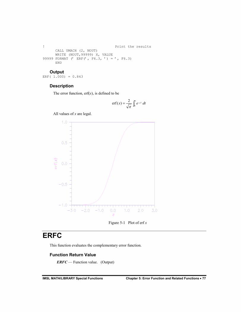
IMSL MATH/LIBRARY Special Functions Chapter 5: Error Function and Related Functions � 77
! Print the results CALL UMACH (2, NOUT) WRITE (NOUT,99999) X, VALUE 99999 FORMAT (� ERF(�, F6.3, �) = �, F6.3) END
Output ERF( 1.000) = 0.843
Description The error function, erf(x), is defined to be
2
0
2erf ( )x
tx e dt�
�� �
All values of x are legal.
Figure 5-1 Plot of erf x
ERFC This function evaluates the complementary error function.
Function Return Value ERFC � Function value. (Output)
78 � Chapter 5: Error Function and Related Functions IMSL MATH LIBRARY /Special Functions
Required Arguments X � Argument for which the function value is desired. (Input)
FORTRAN 90 Interface Generic: ERFC(X)
Specific: The specific interface names are S_ERFC and D_ERFC.
FORTRAN 77 Interface Single: ERFC(X)
Double: The double precision function name is DERFC.
Example In this example, erfc(1.0) is computed and printed.
USE ERFC_INT USE UMACH_INT ! Declare variables INTEGER NOUT REAL VALUE, X ! Compute X = 1.0 VALUE = ERFC(X) ! Print the results CALL UMACH (2, NOUT) WRITE (NOUT,99999) X, VALUE 99999 FORMAT (� ERFC(�, F6.3, �) = �, F6.3) END
Output ERFC( 1.000) = 0.157
Comments Informational error Type Code
2 1 The function underflows because X is too large.
Description The complementary error function, erfc(x), is defined to be
22erfc( ) t
xx e dt
�
�
�� �
The argument x must not be so large that the result underflows. Approximately, x should be less than
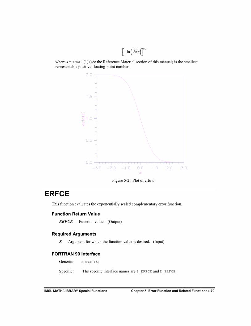
IMSL MATH/LIBRARY Special Functions Chapter 5: Error Function and Related Functions � 79
� �1/ 2
ln s�� ��� �
where s = AMACH(1) (see the Reference Material section of this manual) is the smallest representable positive floating-point number.
Figure 5-2 Plot of erfc x
ERFCE This function evaluates the exponentially scaled complementary error function.
Function Return Value ERFCE � Function value. (Output)
Required Arguments X � Argument for which the function value is desired. (Input)
FORTRAN 90 Interface Generic: ERFCE (X)
Specific: The specific interface names are S_ERFCE and D_ERFCE.
80 � Chapter 5: Error Function and Related Functions IMSL MATH LIBRARY /Special Functions
FORTRAN 77 Interface Single: ERFCE (X)
Double: The double precision function name is DERFCE.
Example In this example, ERFCE(1.0) = e��� erfc(1.0) is computed and printed.
USE ERFCE_INT USE UMACH_INT
! Declare variables INTEGER NOUT REAL VALUE, X ! Compute X = 1.0 VALUE = ERFCE(X) ! Print the results CALL UMACH (2, NOUT) WRITE (NOUT,99999) X, VALUE 99999 FORMAT (� ERFCE(�, F6.3, �) = �, F6.3) END
Output ERFCE( 1.000) = 0.428
Comments Informational error Type Code
2 1 The function underflows because X is too large.
Description The function ERFCE(X) computes
� �2
erfc xe x
where erfc(x) is the complementary error function. See ERFC (page 77) for its definition.
To prevent the answer from underflowing, x must be greater than
min ln( / 2)x b� ��
where b = AMACH(2) is the largest representable floating-point number.
CERFE This function evaluates a scaled function related to ERFC..
IMSL MATH/LIBRARY Special Functions Chapter 5: Error Function and Related Functions � 81
Function Return Value CERFE � Complex function value. (Output)
Required Arguments Z � Complex argument for which the function value is desired. (Input)
FORTRAN 90 Interface Generic: CERFE (Z)
Specific: The specific interface names are C_CERFE and Z_CERFE.
FORTRAN 77 Interface Complex: CERFE (Z)
Double complex: The double complex function name is ZERFE.
Example In this example, CERFE(2.5 + 2.5i) is computed and printed.
USE CERFE_INT USE UMACH_INT ! Declare variables INTEGER NOUT COMPLEX VALUE, Z ! Compute Z = (2.5, 2.5) VALUE = CERFE(Z) ! Print the results CALL UMACH (2, NOUT) WRITE (NOUT,99999) Z, VALUE 99999 FORMAT (� CERFE(�, F6.3, �,�, F6.3, �) = (�, & F6.3, �,�, F6.3, �)�) END
Output CERFE( 2.500, 2.500) = ( 0.117, 0.108)
Description Function CERFCE is defined to be
2 2 22erfc( )z z t
ze iz ie e dt
�
�� �
� � � �
Let b = AMACH(2) be the largest floating-point number. The argument z must satisfy
z b�
82 � Chapter 5: Error Function and Related Functions IMSL MATH LIBRARY /Special Functions
or else the value returned is zero. If the argument z does not satisfy (�z)� � (�z)� � log b, then b is returned. All other arguments are legal (Gautschi 1969, 1970).
ERFI This function evaluates the inverse error function.
Function Return Value ERFI � Function value. (Output)
Required Arguments X � Argument for which the function value is desired. (Input)
FORTRAN 90 Interface Generic: ERFI (X)
Specific: The specific interface names are S_ERFI and D_ERFI.
FORTRAN 77 Interface Single: ERFI (X)
Double: The double precision function name is DERFI.
Example In this example, erf��(erf(1.0)) is computed and printed.
USE ERFI_INT USE ERF_INT USE UMACH_INT
! Declare variables INTEGER NOUT REAL VALUE, X ! Compute X = ERF(1.0) VALUE = ERFI(X) ! Print the results CALL UMACH (2, NOUT) WRITE (NOUT,99999) X, VALUE 99999 FORMAT (� ERFI(�, F6.3, �) = �, F6.3) END
Output ERFI( 0.843) = 1.000
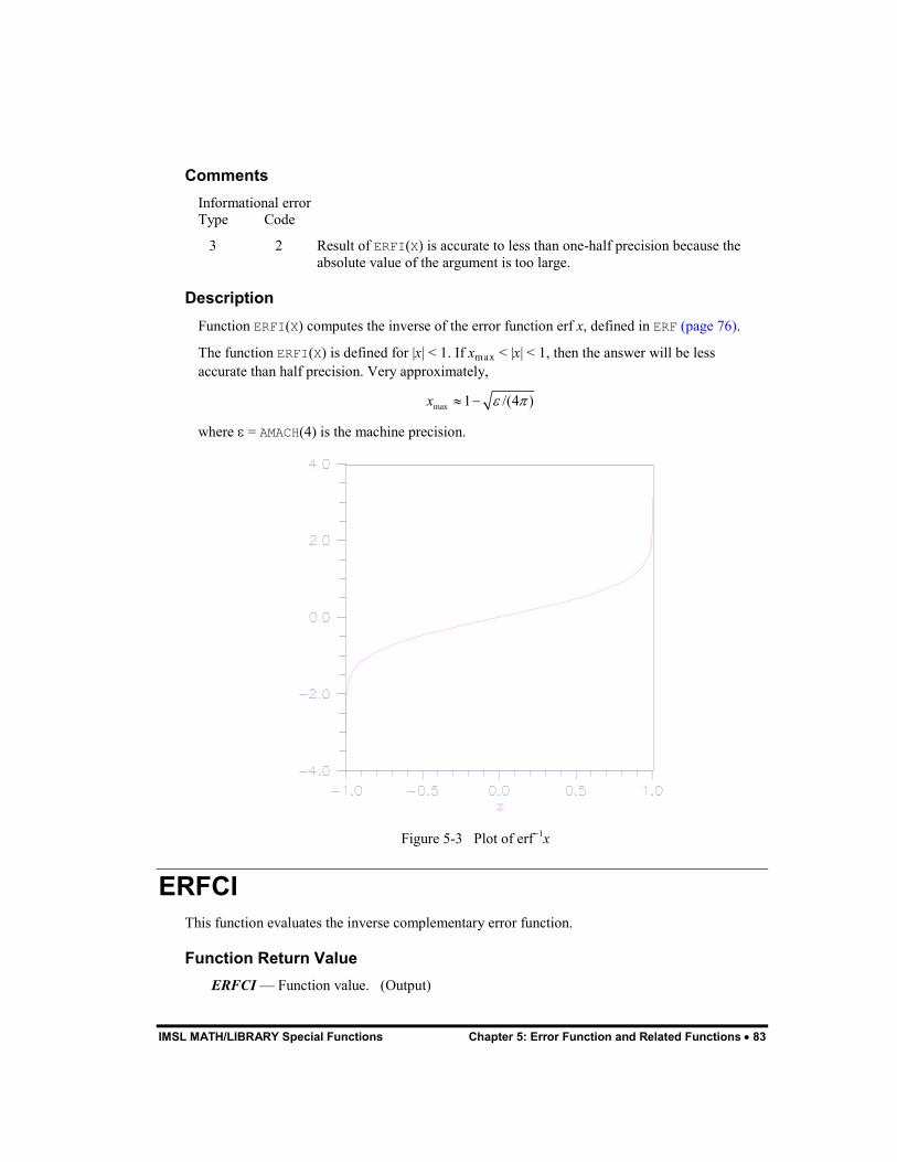
IMSL MATH/LIBRARY Special Functions Chapter 5: Error Function and Related Functions � 83
Comments Informational error Type Code
3 2 Result of ERFI(X) is accurate to less than one-half precision because the absolute value of the argument is too large.
Description Function ERFI(X) computes the inverse of the error function erf x, defined in ERF (page 76).
The function ERFI(X) is defined for |x| < 1. If x� < |x| < 1, then the answer will be less accurate than half precision. Very approximately,
max 1 /(4 )x � �� �
where � = AMACH(4) is the machine precision.
Figure 5-3 Plot of erf��x
ERFCI This function evaluates the inverse complementary error function.
Function Return Value ERFCI � Function value. (Output)

84 � Chapter 5: Error Function and Related Functions IMSL MATH LIBRARY /Special Functions
Required Arguments X � Argument for which the function value is desired. (Input)
FORTRAN 90 Interface Generic: ERFCI (X)
Specific: The specific interface names are S_ERFCI and D_ERFCI.
FORTRAN 77 Interface Single: ERFCI (X)
Double: The double precision function name is DERFCI.
Example In this example, erfc��(erfc(1.0)) is computed and printed.
USE ERFCI_INT USE ERFC_INT USE UMACH_INT
! Declare variables INTEGER NOUT REAL VALUE, X ! Compute X = ERFC(1.0) VALUE = ERFCI(X) ! Print the results CALL UMACH (2, NOUT) WRITE (NOUT,99999) X, VALUE 99999 FORMAT (� ERFCI(�, F6.3, �) = �, F6.3) END
Output ERFCI( 0.157) = 1.000
Comments Informational error Type Code
3 2 Result of ERFCI(X) is accurate to less than one-half precision because the argument is too close to 2.0.
Description The function ERFCI(X) computes the inverse of the complementary error function erfc x, defined in ERFC (page 77).
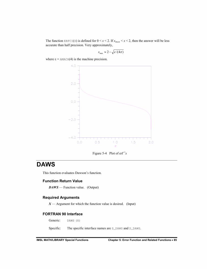
IMSL MATH/LIBRARY Special Functions Chapter 5: Error Function and Related Functions � 85
The function ERFCI(X) is defined for 0 < x < 2. If x� < x < 2, then the answer will be less accurate than half precision. Very approximately,
max 2 /(4 )x � �� �
where � = AMACH(4) is the machine precision.
Figure 5-4 Plot of erf��x
DAWS This function evaluates Dawson�s function.
Function Return Value DAWS � Function value. (Output)
Required Arguments X � Argument for which the function value is desired. (Input)
FORTRAN 90 Interface Generic: DAWS (X)
Specific: The specific interface names are S_DAWS and D_DAWS.
86 � Chapter 5: Error Function and Related Functions IMSL MATH LIBRARY /Special Functions
FORTRAN 77 Interface Single: DAWS (X)
Double: The double precision function name is DDAWS.
Example In this example, DAWS(1.0) is computed and printed.
USE DAWS_INT USE UMACH_INT ! Declare variables INTEGER NOUT REAL VALUE, X ! Compute X = 1.0 VALUE = DAWS(X) ! Print the results CALL UMACH (2, NOUT) WRITE (NOUT,99999) X, VALUE 99999 FORMAT (� DAWS(�, F6.3, �) = �, F6.3) END
Output DAWS( 1.000) = 0.538
Comments 1. Informational error
Type Code
2 1 The function underflows because the absolute value of X is too large.
2. The Dawson function is closely related to the error function for imaginary arguments.
Description Dawson�s function is defined to be
2 2
0
xx te e dt�
�
It is closely related to the error function for imaginary arguments.
So that Dawson�s function does not underflow, |x| must be less than 1/(2s). Here, s = AMACH(1) is the smallest representable positive floating-point number.
FRESC This function evaluates the cosine Fresnel integral.
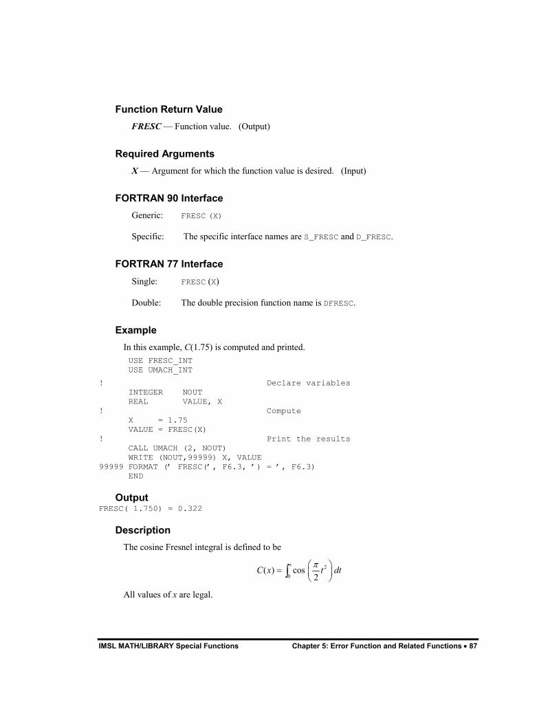
IMSL MATH/LIBRARY Special Functions Chapter 5: Error Function and Related Functions � 87
Function Return Value FRESC � Function value. (Output)
Required Arguments X � Argument for which the function value is desired. (Input)
FORTRAN 90 Interface Generic: FRESC (X)
Specific: The specific interface names are S_FRESC and D_FRESC.
FORTRAN 77 Interface Single: FRESC (X)
Double: The double precision function name is DFRESC.
Example In this example, C(1.75) is computed and printed.
USE FRESC_INT USE UMACH_INT
! Declare variables INTEGER NOUT REAL VALUE, X ! Compute X = 1.75 VALUE = FRESC(X) ! Print the results CALL UMACH (2, NOUT) WRITE (NOUT,99999) X, VALUE 99999 FORMAT (� FRESC(�, F6.3, �) = �, F6.3) END
Output FRESC( 1.750) = 0.322
Description The cosine Fresnel integral is defined to be
2
0( ) cos
2x
C x t dt�� �� � �
� ��
All values of x are legal.
88 � Chapter 5: Error Function and Related Functions IMSL MATH LIBRARY /Special Functions
FRESS This function evaluates the sine Fresnel integral.
Function Value Return FRESS � Function value. (Output)
Required Arguments X � Argument for which the function value is desired. (Input)
FORTRAN 90 Interface Generic: FRESS (X)
Specific: The specific interface names are S_FRESS and D_FRESS.
FORTRAN 77 Interface Single: FRESS (X)
Double: The double precision function name is DFRESS.
Example In this example, S(1.75) is computed and printed.
USE FRESS_INT USE UMACH_INT ! Declare variables INTEGER NOUT REAL VALUE, X ! Compute X = 1.75 VALUE = FRESS(X) ! Print the results CALL UMACH (2, NOUT) WRITE (NOUT,99999) X, VALUE 99999 FORMAT (� FRESS(�, F6.3, �) = �, F6.3) END
Output FRESS( 1.750) = 0.499

IMSL MATH/LIBRARY Special Functions Chapter 5: Error Function and Related Functions � 89
Description The sine Fresnel integral is defined to be
2
0( ) sin
2x
S x t dt�� �� � �
� ��
All values of x are legal.

90 � Chapter 5: Error Function and Related Functions IMSL MATH LIBRARY /Special Functions
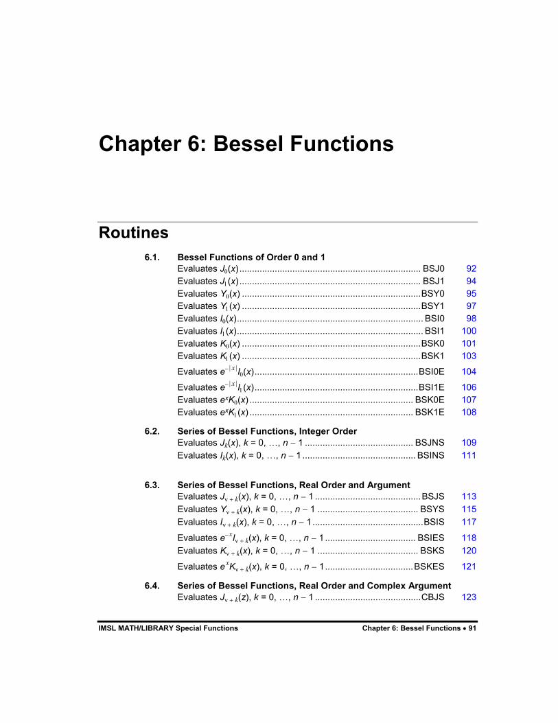
IMSL MATH/LIBRARY Special Functions Chapter 6: Bessel Functions � 91
Chapter 6: Bessel Functions
Routines 6.1. Bessel Functions of Order 0 and 1
Evaluates J�(x) ........................................................................ BSJ0 92 Evaluates J�(x) ........................................................................ BSJ1 94 Evaluates Y�(x) .......................................................................BSY0 95 Evaluates Y�(x) .......................................................................BSY1 97 Evaluates I�(x).......................................................................... BSI0 98 Evaluates I�(x).......................................................................... BSI1 100 Evaluates K�(x) .......................................................................BSK0 101 Evaluates K�(x) .......................................................................BSK1 103
Evaluates e�|x|I�(x).................................................................BSI0E 104
Evaluates e�|x|I�(x).................................................................BSI1E 106 Evaluates exK�(x) ................................................................. BSK0E 107 Evaluates exK�(x) ................................................................. BSK1E 108
6.2. Series of Bessel Functions, Integer Order Evaluates Jk(x), k = 0, �, n � 1 ........................................... BSJNS 109 Evaluates Ik(x), k = 0, �, n � 1 ............................................. BSINS 111
6.3. Series of Bessel Functions, Real Order and Argument Evaluates J� � k(x), k = 0, �, n � 1 ..........................................BSJS 113 Evaluates Y� � k(x), k = 0, �, n � 1 ........................................ BSYS 115 Evaluates I� � k(x), k = 0, �, n � 1 ............................................BSIS 117
Evaluates e�xI� � k(x), k = 0, �, n � 1 .................................... BSIES 118 Evaluates K� � k(x), k = 0, �, n � 1 ........................................ BSKS 120
Evaluates exK� � k(x), k = 0, �, n � 1...................................BSKES 121
6.4. Series of Bessel Functions, Real Order and Complex Argument Evaluates J� � k(z), k = 0, �, n � 1 ..........................................CBJS 123
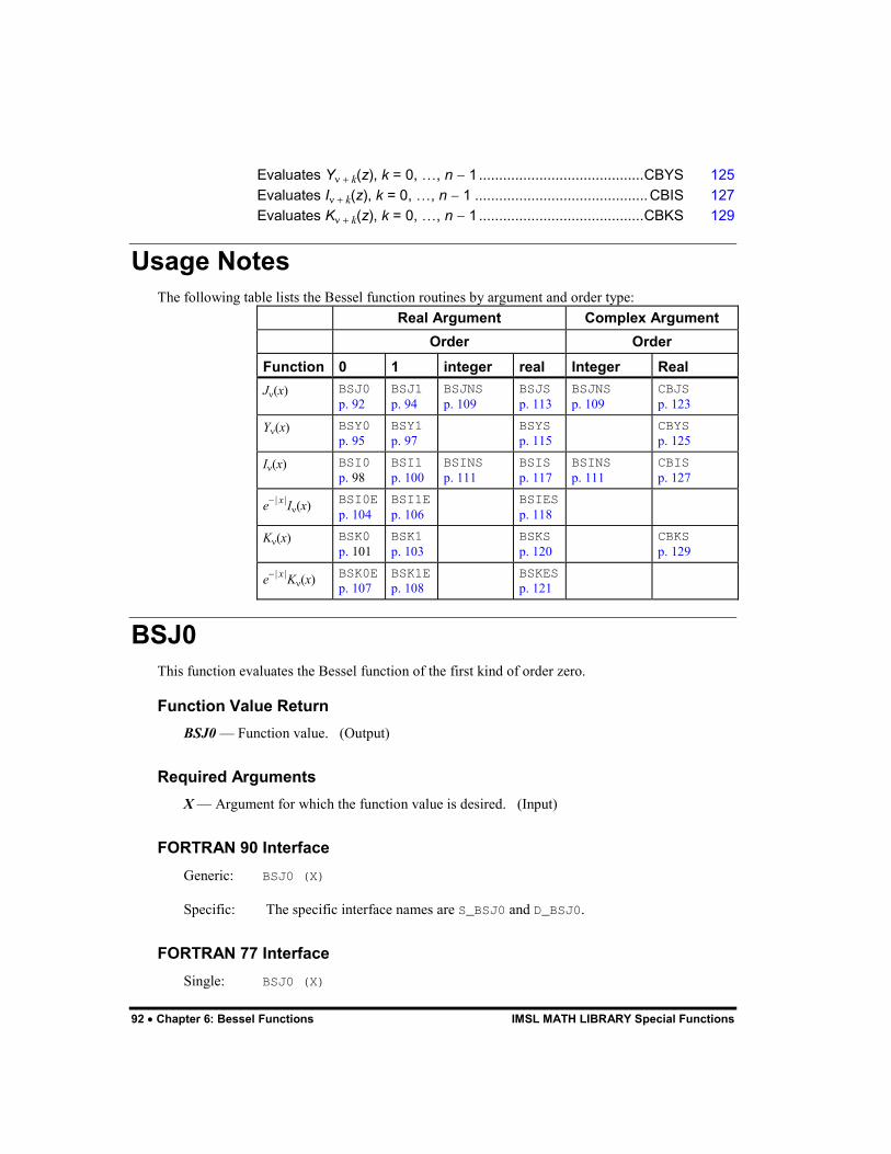
92 � Chapter 6: Bessel Functions IMSL MATH LIBRARY Special Functions
Evaluates Y� � k(z), k = 0, �, n � 1 .........................................CBYS 125 Evaluates I� � k(z), k = 0, �, n � 1 ...........................................CBIS 127 Evaluates K� � k(z), k = 0, �, n � 1 .........................................CBKS 129
Usage Notes The following table lists the Bessel function routines by argument and order type:
Real Argument Complex Argument Order Order Function 0 1 integer real Integer Real J�(x) BSJ0
p. 92 BSJ1 p. 94
BSJNS p. 109
BSJS p. 113
BSJNS p. 109
CBJS p. 123
Y�(x) BSY0 p. 95
BSY1 p. 97
BSYS p. 115
CBYS p. 125
I�(x) BSI0 p. 98
BSI1 p. 100
BSINS p. 111
BSIS p. 117
BSINS p. 111
CBIS p. 127
e�|x|I�(x) BSI0Ep. 104
BSI1Ep. 106
BSIESp. 118
K�(x) BSK0 p. 101
BSK1 p. 103
BSKS p. 120
CBKS p. 129
e�|x|K�(x) BSK0Ep. 107
BSK1Ep. 108
BSKESp. 121
BSJ0 This function evaluates the Bessel function of the first kind of order zero.
Function Value Return BSJ0 � Function value. (Output)
Required Arguments X � Argument for which the function value is desired. (Input)
FORTRAN 90 Interface Generic: BSJ0 (X)
Specific: The specific interface names are S_BSJ0 and D_BSJ0.
FORTRAN 77 Interface Single: BSJ0 (X)
IMSL MATH/LIBRARY Special Functions Chapter 6: Bessel Functions � 93
Double: The double precision function name is DBSJ0.
Example In this example, J�(3.0) is computed and printed.
USE BSJ0_INT USE UMACH_INT
! Declare variables INTEGER NOUT REAL VALUE, X ! Compute X = 3.0 VALUE = BSJ0(X) ! Print the results CALL UMACH (2, NOUT) WRITE (NOUT,99999) X, VALUE 99999 FORMAT (� BSJ0(�, F6.3, �) = �, F6.3) END
Output BSJ0( 3.000) = -0.260
Description The Bessel function J�(x) is defined to be
� � � �0 0
1 cos sinJ x x d�
� ��
� �
To prevent the answer from being less accurate than half precision, |x| should be smaller than
1/ �
For the result to have any precision at all, |x| must be less than 1/�. Here, � is the machine precision, � = AMACH(4).

94 � Chapter 6: Bessel Functions IMSL MATH LIBRARY Special Functions
Figure 6-1 Plot of J�(x) and J�(x)
BSJ1 This function evaluates the Bessel function of the first kind of order one.
Function Return Value BSJ1 � Function value. (Output)
Required Arguments X � Argument for which the function value is desired. (Input)
FORTRAN 90 Interface Generic: BSJ1 (X)
Specific: The specific interface names are S_BSJ1 and D_BSJ1.
FORTRAN 77 Interface Single: BSJ1 (X)
Double: The double precision function name is DBSJ1.
IMSL MATH/LIBRARY Special Functions Chapter 6: Bessel Functions � 95
Example In this example, J�(2.5) is computed and printed.
USE BSJ1_INT USE UMACH_INT ! Declare variables INTEGER NOUT REAL VALUE, X ! Compute X = 2.5 VALUE = BSJ1(X) ! Print the results CALL UMACH (2, NOUT) WRITE (NOUT,99999) X, VALUE 99999 FORMAT (� BSJ1(�, F6.3, �) = �, F6.3) END
Output BSJ1( 2.500) = 0.497
Comments Informational error Type Code
2 1 The function underflows because the absolute value of X is too small.
Description The Bessel function J�(x) is defined to be
� � � �1 0
1 cos sinθ θ θJ x x d�
�� ��
The argument x must be zero or larger in absolute value than 2s to prevent J�(x) from underflowing. Also, |x| should be smaller than
1/ �
to prevent the answer from being less accurate than half precision. |x| must be less than 1/� for the result to have any precision at all. Here, � is the machine precision, � = AMACH(4), and s = AMACH(1) is the smallest representable positive floating-point number.
BSY0 This function evaluates the Bessel function of the second kind of order zero.
Function Return Value BSY0 � Function value. (Output)
96 � Chapter 6: Bessel Functions IMSL MATH LIBRARY Special Functions
Required Arguments X � Argument for which the function value is desired. (Input)
FORTRAN 90 Interface Generic: BSY0 (X)
Specific: The specific interface names are S_BSY0 and D_BSY0.
FORTRAN 77 Interface Single: BSY0 (X)
Double: The double precision function name is DBSY0.
Example In this example, Y�(3.0) is computed and printed.
USE BSY0_INT USE UMACH_INT
! Declare variables INTEGER NOUT REAL VALUE, X ! Compute X = 3.0 VALUE = BSY0(X) ! Print the results CALL UMACH (2, NOUT) WRITE (NOUT,99999) X, VALUE 99999 FORMAT (� BSY0(�, F6.3, �) = �, F6.3) END
Output BSY0( 3.000) = 0.377
Description The Bessel function Y�(x) is defined to be
� � � � sinh0 0 0
1 2sin sin z tY x x d e dt�
� �� �
��
� �� �
To prevent the answer from being less accurate than half precision, x should be smaller than
1/ �
For the result to have any precision at all, |x| must be less than 1/�. Here, � is the machine precision, � = AMACH(4).
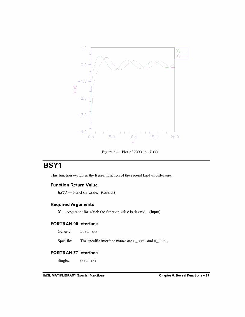
IMSL MATH/LIBRARY Special Functions Chapter 6: Bessel Functions � 97
Figure 6-2 Plot of Y�(x) and Y�(x)
BSY1 This function evaluates the Bessel function of the second kind of order one.
Function Return Value BSY1 � Function value. (Output)
Required Arguments X � Argument for which the function value is desired. (Input)
FORTRAN 90 Interface Generic: BSY1 (X)
Specific: The specific interface names are S_BSY1 and D_BSY1.
FORTRAN 77 Interface Single: BSY1 (X)
98 � Chapter 6: Bessel Functions IMSL MATH LIBRARY Special Functions
Double: The double precision function name is DBSY1.
Example In this example, Y�(3.0) is computed and printed.
USE BSY1_INT USE UMACH_INT ! Declare variables INTEGER NOUT REAL VALUE, X ! Compute X = 3.0 VALUE = BSY1(X) ! Print the results CALL UMACH (2, NOUT) WRITE (NOUT,99999) X, VALUE 99999 FORMAT (� BSY1(�, F6.3, �) = �, F6.3) END
Output BSY1( 3.000) = 0.325
Description The Bessel function Y�(x) is defined to be
� � � � � � sinh1 0 0
1 1sin sin t t z tY x x d e e e dt�
� � �� �
�� �
� � � � �� �
Y�(x) is defined for x > 0. To prevent the answer from being less accurate than half precision, x should be smaller than
1/ �
For the result to have any precision at all, |x| must be less than 1/�. Here, � is the machine precision, � = AMACH(4).
BSI0 This function evaluates the modified Bessel function of the first kind of order zero.
Function Return Value BSI0 � Function value. (Output)
Required Arguments X � Argument for which the function value is desired. (Input)
IMSL MATH/LIBRARY Special Functions Chapter 6: Bessel Functions � 99
FORTRAN 90 Interface Generic: BSI0 (X)
Specific: The specific interface names are S_BSI0 and D_BSI0.
FORTRAN 77 Interface Single: BSI0 (X)
Double: The double precision function name is DBSI0.
Example In this example, I�(4.5) is computed and printed.
USE BSI0_INT USE UMACH_INT
! Declare variables INTEGER NOUT REAL VALUE, X ! Compute X = 4.5 VALUE = BSI0(X) ! Print the results CALL UMACH (2, NOUT) WRITE (NOUT,99999) X, VALUE 99999 FORMAT (� BSI0(�, F6.3, �) = �, F6.3) END
Output BSI0( 4.500) = 17.481
Description The Bessel function I�(x) is defined to be
� � � �0 0
1 cosh cosI x x d�
� ��
� �
The absolute value of the argument x must not be so large that e|x| overflows.
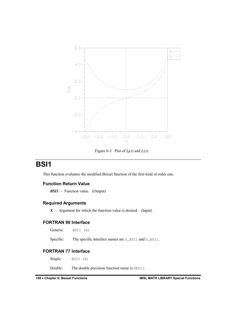
100 � Chapter 6: Bessel Functions IMSL MATH LIBRARY Special Functions
Figure 6-3 Plot of I�(x) and I�(x)
BSI1 This function evaluates the modified Bessel function of the first kind of order one.
Function Return Value BSI1 � Function value. (Output)
Required Arguments X � Argument for which the function value is desired. (Input)
FORTRAN 90 Interface Generic: BSI1 (X)
Specific: The specific interface names are S_BSI1 and D_BSI1.
FORTRAN 77 Interface Single: BSI1 (X)
Double: The double precision function name is DBSI1.
IMSL MATH/LIBRARY Special Functions Chapter 6: Bessel Functions � 101
Example In this example, I�(4.5) is computed and printed.
USE BSI1_INT USE UMACH_INT ! Declare variables INTEGER NOUT REAL VALUE, X ! Compute X = 4.5 VALUE = BSI1(X) ! Print the results CALL UMACH (2, NOUT) WRITE (NOUT,99999) X, VALUE 99999 FORMAT (� BSI1(�, F6.3, �) = �, F6.3) END
Output BSI1( 4.500) = 15.389
Comments Informational error Type Code
2 1 The function underflows because the absolute value of X is too small.
Description The Bessel function I�(x) is defined to be
� � cosθ1 0
1 e cosθ θxI x d�
�
� �
The argument should not be so close to zero that I�(x) � x/2 underflows, nor so large in absolute
value that e|x| and, therefore, I�(x) overflows.
BSK0 This function evaluates the modified Bessel function of the second kind of order zero.
Function Return Value BSK0 � Function value. (Output)
Required Arguments X � Argument for which the function value is desired. (Input)
102 � Chapter 6: Bessel Functions IMSL MATH LIBRARY Special Functions
FORTRAN 90 Interface Generic: BSK0 (X)
Specific: The specific interface names are S_BSK0 and D_BSK0.
FORTRAN 77 Interface Single: BSK0 (X)
Double: The double precision function name is DBSK0.
Example In this example, K�(0.5) is computed and printed.
USE BSK0_INT USE UMACH_INT ! Declare variables INTEGER NOUT REAL VALUE, X ! Compute X = 0.5 VALUE = BSK0(X) ! Print the results CALL UMACH (2, NOUT) WRITE (NOUT,99999) X, VALUE 99999 FORMAT (� BSK0(�, F6.3, �) = �, F6.3) END
Output BSK0( 0.500) = 0.924
Comments Informational error Type Code
2 1 The function underflows because X is too large.
Description The Bessel function K�(x) is defined to be
� � � �0 0cos sinhK x x t dt
�
� �
The argument must be larger than zero, but not so large that the result, approximately equal to
� �/ 2 xx e��
underflows.
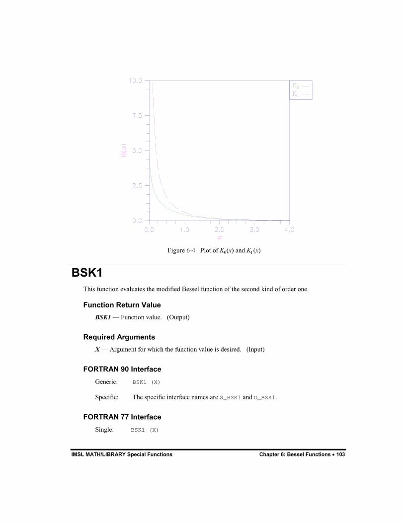
IMSL MATH/LIBRARY Special Functions Chapter 6: Bessel Functions � 103
Figure 6-4 Plot of K�(x) and K�(x)
BSK1 This function evaluates the modified Bessel function of the second kind of order one.
Function Return Value BSK1 � Function value. (Output)
Required Arguments X � Argument for which the function value is desired. (Input)
FORTRAN 90 Interface Generic: BSK1 (X)
Specific: The specific interface names are S_BSK1 and D_BSK1.
FORTRAN 77 Interface Single: BSK1 (X)
104 � Chapter 6: Bessel Functions IMSL MATH LIBRARY Special Functions
Double: The double precision function name is DBSK1.
Example In this example, K�(0.5) is computed and printed.
USE BSK1_INT USE UMACH_INT ! Declare variables INTEGER NOUT REAL VALUE, X ! Compute X = 0.5 VALUE = BSK1(X) ! Print the results CALL UMACH (2, NOUT) WRITE (NOUT,99999) X, VALUE 99999 FORMAT (� BSK1(�, F6.3, �) = �, F6.3) END
Output BSK1( 0.500) = 1.656
Comments Informational error Type Code
2 1 The function underflows because X is too large.
Description The Bessel function K�(x) is defined to be
� � � �1 0sin sinh sinhK x x t t dt
�
� �
The argument x must be large enough (> max(1/b, s)) that K�(x) does not overflow, and x must be small enough that the approximate answer,
� �/ 2 xx e��
does not underflow. Here, s is the smallest representable positive floating-point number, s = AMACH(1) , and b = AMACH(2) is the largest representable floating-point number.
BSI0E This function evaluates the exponentially scaled modified Bessel function of the first kind of order zero.

IMSL MATH/LIBRARY Special Functions Chapter 6: Bessel Functions � 105
Function Return Value BSI0E � Function value. (Output)
Required Arguments X � Argument for which the function value is desired. (Input)
FORTRAN 90 Interface Generic: BSI0E (X)
Specific: The specific interface names are S_BSI0E and D_BSI0E.
FORTRAN 77 Interface Single: BSI0E (X)
Double: The double precision function name is DBSI0E.
Example In this example, BSI0E(4.5) is computed and printed.
USE BSI0E_INT USE UMACH_INT ! Declare variables INTEGER NOUT REAL VALUE, X ! Compute X = 4.5 VALUE = BSI0E(X) ! Print the results CALL UMACH (2, NOUT) WRITE (NOUT,99999) X, VALUE 99999 FORMAT (� BSI0E(�, F6.3, �) = �, F6.3) END
Output BSI0E( 4.500) = 0.194
Description
Function BSI0E computes e�|x| I�(x). For the definition of the Bessel function I�(x), see BSI0 (page 98).
106 � Chapter 6: Bessel Functions IMSL MATH LIBRARY Special Functions
BSI1E This function evaluates the exponentially scaled modified Bessel function of the first kind of order one.
Function Return Value BSI1E � Function value. (Output)
Required Arguments X � Argument for which the function value is desired. (Input)
FORTRAN 90 Interface Generic: BSI1E (X)
Specific: The specific interface names are S_BSI1E and D_BSI1E.
FORTRAN 77 Interface Single: BSI1E (X)
Double: The double precision function name is DBSI1E.
Example In this example, BSI1E(4.5) is computed and printed.
USE BSI1E_INT USE UMACH_INT ! Declare variables INTEGER NOUT REAL VALUE, X ! Compute X = 4.5 VALUE = BSI1E(X) ! Print the results CALL UMACH (2, NOUT) WRITE (NOUT,99999) X, VALUE 99999 FORMAT (� BSI1E(�, F6.3, �) = �, F6.3) END
Output BSI1E( 4.500) = 0.171
Comments Informational error Type Code
IMSL MATH/LIBRARY Special Functions Chapter 6: Bessel Functions � 107
2 1 The function underflows because the absolute value of X is too small.
Description
Function BSI1E computes e�|x| I�(x). For the definition of the Bessel function I�(x), see BSI1 (page 100). The function BSI1E underflows if |x|/2 underflows.
BSK0E This function evaluates the exponentially scaled modified Bessel function of the second kind of order zero.
Function Return Value BSK0E � Function value. (Output)
Required Arguments X � Argument for which the function value is desired. (Input)
FORTRAN 90 Interface Generic: BSK0E (X)
Specific: The specific interface names are S_BSK0E and D_BSK0E.
FORTRAN 77 Interface Single: BSK0E (X)
Double: The double precision function name is DBSK0E.
Example In this example, BSK0E(0.5) is computed and printed.
USE BSK0E_INT USE UMACH_INT ! Declare variables INTEGER NOUT REAL VALUE, X ! Compute X = 0.5 VALUE = BSK0E(X) ! Print the results CALL UMACH (2, NOUT) WRITE (NOUT,99999) X, VALUE 99999 FORMAT (� BSK0E(�, F6.3, �) = �, F6.3) END
108 � Chapter 6: Bessel Functions IMSL MATH LIBRARY Special Functions
Output BSK0E( 0.500) = 1.524
Description
Function BSK0E computes exK�(x). For the definition of the Bessel function K�(x), see BSK0 (page 101). The argument must be greater than zero for the result to be defined.
BSK1E This function evaluates the exponentially scaled modified Bessel function of the second kind of order one.
Function Return Value BSK1E � Function value. (Output)
Required Arguments X � Argument for which the function value is desired. (Input)
FORTRAN 90 Interface Generic: BSK1E (X)
Specific: The specific interface names are S_BSK1E and D_BSK1E.
FORTRAN 77 Interface Single: BSK1E (X)
Double: The double precision function name is DBSK1E.
Example In this example, BSK1E(0.5) is computed and printed.
USE BSK1E_INT USE UMACH_INT ! Declare variables INTEGER NOUT REAL VALUE, X ! Compute X = 0.5 VALUE = BSK1E(X) ! Print the results CALL UMACH (2, NOUT) WRITE (NOUT,99999) X, VALUE 99999 FORMAT (� BSK1E(�, F6.3, �) = �, F6.3) END
IMSL MATH/LIBRARY Special Functions Chapter 6: Bessel Functions � 109
Output BSK1E( 0.500) = 2.731
Description
Function BSK1E computes exK�(x). For the definition of the Bessel function K�(x), see BSK1
(page 103). The answer BSK1E = exK�(x) � 1/x overflows if x is too close to zero.
BSJNS Evaluates a sequence of Bessel functions of the first kind with integer order and real or complex arguments.
Required Arguments X � Argument for which the sequence of Bessel functions is to be evaluated. (Input)
The absolute value of real arguments must be less than 10�. The absolute value of complex arguments must be less than 10�.
N � Number of elements in the sequence. (Input) It must be a positive integer.
BS � Vector of length N containing the values of the function through the series. (Output) BS(I) contains the value of the Bessel function of order I � 1 at x for I = 1 to N.
FORTRAN 90 Interface Generic: CALL BSJNS (X, N, BS)
Specific: The specific interface names are S_BSJNS, D_BSJNS, C_BSJNS, and Z_BSJNS
FORTRAN 77 Interface Single: CALL BSJNS (X, N, BS)
Double: The double precision name is DBSJNS.
Complex: The complex name is CBJNS.
Double Complex: The double complex name is DCBJNS.
Example In this example, Jn(10.0), n = 0, �, 9 is computed and printed.
110 � Chapter 6: Bessel Functions IMSL MATH LIBRARY Special Functions
USE BSJNS_INT USE UMACH_INT ! Declare variables INTEGER N PARAMETER (N=10) ! INTEGER K, NOUT REAL BS(N), X ! Compute X = 10.0 CALL BSJNS (X, N, BS) ! Print the results CALL UMACH (2, NOUT) DO 10 K=1, N WRITE (NOUT,99999) K-1, X, BS(K) 10 CONTINUE 99999 FORMAT (� J sub �, I2, � (�, F6.3, �) = �, F6.3) END
Output J sub 0 (10.000) = -0.246 J sub 1 (10.000) = 0.043 J sub 2 (10.000) = 0.255 J sub 3 (10.000) = 0.058 J sub 4 (10.000) = -0.220 J sub 5 (10.000) = -0.234 J sub 6 (10.000) = -0.014 J sub 7 (10.000) = 0.217 J sub 8 (10.000) = 0.318 J sub 9 (10.000) = 0.292
Description The complex Bessel function Jn(z) is defined to be
� � � �0
1 cos sinnJ z z n d�
� � ��
� ��
This code is based on the work of Sookne (1973a) and Olver and Sookne (1972). It uses backward recursion with strict error control.
Additional Example In this example, Jn(10 + 10i), n = 0, �, 10 is computed and printed.
USE BSJNS_INT USE UMACH_INT ! Declare variables INTEGER N PARAMETER (N=11) ! INTEGER K, NOUT COMPLEX CBS(N), Z ! Compute Z = (10.0, 10.0)

IMSL MATH/LIBRARY Special Functions Chapter 6: Bessel Functions � 111
CALL BSJNS (Z, N, CBS) ! Print the results CALL UMACH (2, NOUT) DO 10 K=1, N WRITE (NOUT,99999) K-1, Z, CBS(K) 10 CONTINUE 99999 FORMAT (� J sub �, I2, � ((�, F6.3, �,�, F6.3, & �)) = (�, F9.3, �,�, F9.3, �)�) END
Output J sub 0 ((10.000,10.000)) = (-2314.975, 411.563) J sub 1 ((10.000,10.000)) = ( -460.681,-2246.627) J sub 2 ((10.000,10.000)) = ( 2044.245, -590.157) J sub 3 ((10.000,10.000)) = ( 751.498, 1719.746) J sub 4 ((10.000,10.000)) = (-1302.871, 880.632) J sub 5 ((10.000,10.000)) = ( -920.394, -846.345) J sub 6 ((10.000,10.000)) = ( 419.501, -843.607) J sub 7 ((10.000,10.000)) = ( 665.930, 88.480) J sub 8 ((10.000,10.000)) = ( 108.586, 439.392) J sub 9 ((10.000,10.000)) = ( -227.548, 176.165) J sub 10 ((10.000,10.000)) = ( -154.831, -76.050)
BSINS Evaluates a sequence of modified Bessel functions of the first kind with integer order and real or complex arguments.
Required Arguments X � Argument for which the sequence of Bessel functions is to be evaluated. (Input)
For real argument exp(|x|) must not overflow. For complex arguments x must be less than 10� in absolute value.
N � Number of elements in the sequence. (Input)
BSI � Vector of length N containing the values of the function through the series. (Output) BSI(I) contains the value of the Bessel function of order I � 1 at x for I = 1 to N.
FORTRAN 90 Interface Generic: CALL BSINS (X, N, BSI)
Specific: The specific interface names are S_BSINS, D_BSINS, C_BSINS, and Z_BSINS.
FORTRAN 77 Interface Single: CALL BSINS (X, N, BSI)
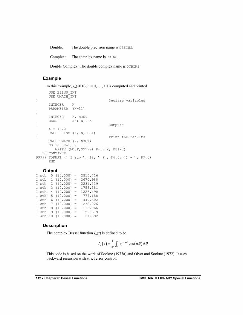
112 � Chapter 6: Bessel Functions IMSL MATH LIBRARY Special Functions
Double: The double precision name is DBSINS.
Complex: The complex name is CBINS.
Double Complex: The double complex name is DCBINS.
Example In this example, In(10.0), n = 0, �, 10 is computed and printed.
USE BSINS_INT USE UMACH_INT ! Declare variables INTEGER N PARAMETER (N=11) ! INTEGER K, NOUT REAL BSI(N), X ! Compute X = 10.0 CALL BSINS (X, N, BSI) ! Print the results CALL UMACH (2, NOUT) DO 10 K=1, N WRITE (NOUT,99999) K-1, X, BSI(K) 10 CONTINUE 99999 FORMAT (� I sub �, I2, � (�, F6.3, �) = �, F9.3) END
Output I sub 0 (10.000) = 2815.716 I sub 1 (10.000) = 2670.988 I sub 2 (10.000) = 2281.519 I sub 3 (10.000) = 1758.381 I sub 4 (10.000) = 1226.490 I sub 5 (10.000) = 777.188 I sub 6 (10.000) = 449.302 I sub 7 (10.000) = 238.026 I sub 8 (10.000) = 116.066 I sub 9 (10.000) = 52.319 I sub 10 (10.000) = 21.892
Description The complex Bessel function In(z) is defined to be
� � � �cos
0
1 cosznI z e n d
��
� ��
� �
This code is based on the work of Sookne (1973a) and Olver and Sookne (1972). It uses backward recursion with strict error control.
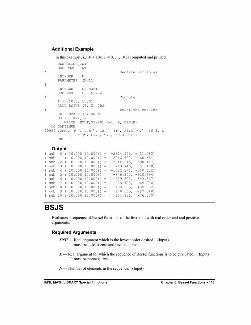
IMSL MATH/LIBRARY Special Functions Chapter 6: Bessel Functions � 113
Additional Example In this example, In(10 + 10i), n = 0, �, 10 is computed and printed.
USE BSINS_INT USE UMACH_INT ! Declare variables INTEGER N PARAMETER (N=11) ! INTEGER K, NOUT COMPLEX CBS(N), Z ! Compute Z = (10.0, 10.0) CALL BSINS (Z, N, CBS) ! Print the results CALL UMACH (2, NOUT) DO 10 K=1, N WRITE (NOUT,99999) K-1, Z, CBS(K) 10 CONTINUE 99999 FORMAT (� I sub �, I2, � ((�, F6.3, �,�, F6.3, & �)) = (�, F9.3, �,�, F9.3, �)�) END
Output I sub 0 ((10.000,10.000)) = (-2314.975, -411.563) I sub 1 ((10.000,10.000)) = (-2246.627, -460.681) I sub 2 ((10.000,10.000)) = (-2044.245, -590.157) I sub 3 ((10.000,10.000)) = (-1719.746, -751.498) I sub 4 ((10.000,10.000)) = (-1302.871, -880.632) I sub 5 ((10.000,10.000)) = ( -846.345, -920.394) I sub 6 ((10.000,10.000)) = ( -419.501, -843.607) I sub 7 ((10.000,10.000)) = ( -88.480, -665.930) I sub 8 ((10.000,10.000)) = ( 108.586, -439.392) I sub 9 ((10.000,10.000)) = ( 176.165, -227.548) I sub 10 ((10.000,10.000)) = ( 154.831, -76.050)
BSJS Evaluates a sequence of Bessel functions of the first kind with real order and real positive arguments.
Required Arguments XNU � Real argument which is the lowest order desired. (Input)
It must be at least zero and less than one.
X � Real argument for which the sequence of Bessel functions is to be evaluated. (Input) It must be nonnegative.
N � Number of elements in the sequence. (Input)
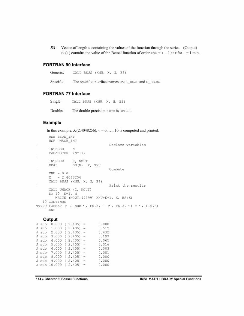
114 � Chapter 6: Bessel Functions IMSL MATH LIBRARY Special Functions
BS � Vector of length N containing the values of the function through the series. (Output) BS(I) contains the value of the Bessel function of order XNU + I � 1 at x for I = 1 to N.
FORTRAN 90 Interface Generic: CALL BSJS (XNU, X, N, BS)
Specific: The specific interface names are S_BSJS and D_BSJS.
FORTRAN 77 Interface Single: CALL BSJS (XNU, X, N, BS)
Double: The double precision name is DBSJS.
Example In this example, J�(2.4048256), � = 0, �, 10 is computed and printed.
USE BSJS_INT USE UMACH_INT ! Declare variables INTEGER N PARAMETER (N=11) ! INTEGER K, NOUT REAL BS(N), X, XNU ! Compute XNU = 0.0 X = 2.4048256 CALL BSJS (XNU, X, N, BS) ! Print the results CALL UMACH (2, NOUT) DO 10 K=1, N WRITE (NOUT,99999) XNU+K-1, X, BS(K) 10 CONTINUE 99999 FORMAT (� J sub �, F6.3, � (�, F6.3, �) = �, F10.3) END
Output J sub 0.000 ( 2.405) = 0.000 J sub 1.000 ( 2.405) = 0.519 J sub 2.000 ( 2.405) = 0.432 J sub 3.000 ( 2.405) = 0.199 J sub 4.000 ( 2.405) = 0.065 J sub 5.000 ( 2.405) = 0.016 J sub 6.000 ( 2.405) = 0.003 J sub 7.000 ( 2.405) = 0.001 J sub 8.000 ( 2.405) = 0.000 J sub 9.000 ( 2.405) = 0.000 J sub 10.000 ( 2.405) = 0.000
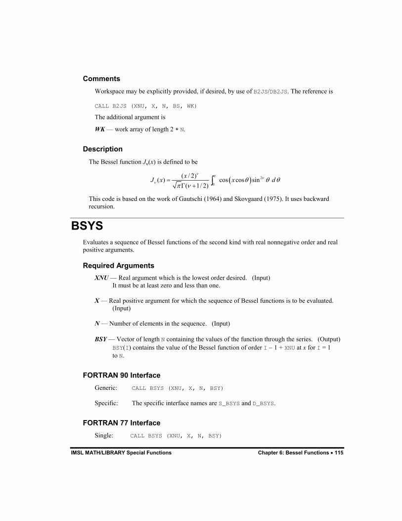
IMSL MATH/LIBRARY Special Functions Chapter 6: Bessel Functions � 115
Comments Workspace may be explicitly provided, if desired, by use of B2JS/DB2JS. The reference is
CALL B2JS (XNU, X, N, BS, WK)
The additional argument is
WK � work array of length 2 � N.
Description The Bessel function J�(x) is defined to be
� � 2
0
( / 2)( ) cos cos sin( 1/ 2)xJ x x d
��
�
�� � �
� ��
� ��
This code is based on the work of Gautschi (1964) and Skovgaard (1975). It uses backward recursion.
BSYS Evaluates a sequence of Bessel functions of the second kind with real nonnegative order and real positive arguments.
Required Arguments XNU � Real argument which is the lowest order desired. (Input)
It must be at least zero and less than one.
X � Real positive argument for which the sequence of Bessel functions is to be evaluated. (Input)
N � Number of elements in the sequence. (Input)
BSY � Vector of length N containing the values of the function through the series. (Output) BSY(I) contains the value of the Bessel function of order I � 1 + XNU at x for I = 1 to N.
FORTRAN 90 Interface Generic: CALL BSYS (XNU, X, N, BSY)
Specific: The specific interface names are S_BSYS and D_BSYS.
FORTRAN 77 Interface Single: CALL BSYS (XNU, X, N, BSY)
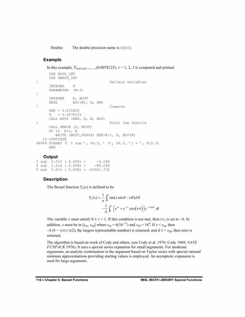
116 � Chapter 6: Bessel Functions IMSL MATH LIBRARY Special Functions
Double: The double precision name is DBSYS.
Example In this example, Y�������� � � �(0.0078125), � = 1, 2, 3 is computed and printed.
USE BSYS_INT USE UMACH_INT ! Declare variables INTEGER N PARAMETER (N=3) ! INTEGER K, NOUT REAL BSY(N), X, XNU ! Compute XNU = 0.015625 X = 0.0078125 CALL BSYS (XNU, X, N, BSY) ! Print the results CALL UMACH (2, NOUT) DO 10 K=1, N WRITE (NOUT,99999) XNU+K-1, X, BSY(K) 10 CONTINUE 99999 FORMAT (� Y sub �, F6.3, � (�, F6.3, �) = �, F10.3) END
Output Y sub 0.016 ( 0.008) = -3.189 Y sub 1.016 ( 0.008) = -88.096 Y sub 2.016 ( 0.008) = -22901.732
Description The Bessel function Y�(x) is defined to be
� �
0
sinh
0
1( ) sin( sin )
1 cost t x t
Y x x d
e e e dt
�
�
� �
� �� ��
���
�� �
� �
� �� �� �
�
�
The variable � must satisfy 0 � � < 1. If this condition is not met, then BSi is set to �b. In addition, x must be in [xm, xM] where xm = 6(16���) and xM = 16�. If x < xm, then �b (b = AMACH(2), the largest representable number) is returned; and if x > xM, then zero is returned.
The algorithm is based on work of Cody and others, (see Cody et al. 1976; Cody 1969; NATS FUNPACK 1976). It uses a special series expansion for small arguments. For moderate arguments, an analytic continuation in the argument based on Taylor series with special rational minimax approximations providing starting values is employed. An asymptotic expansion is used for large arguments.
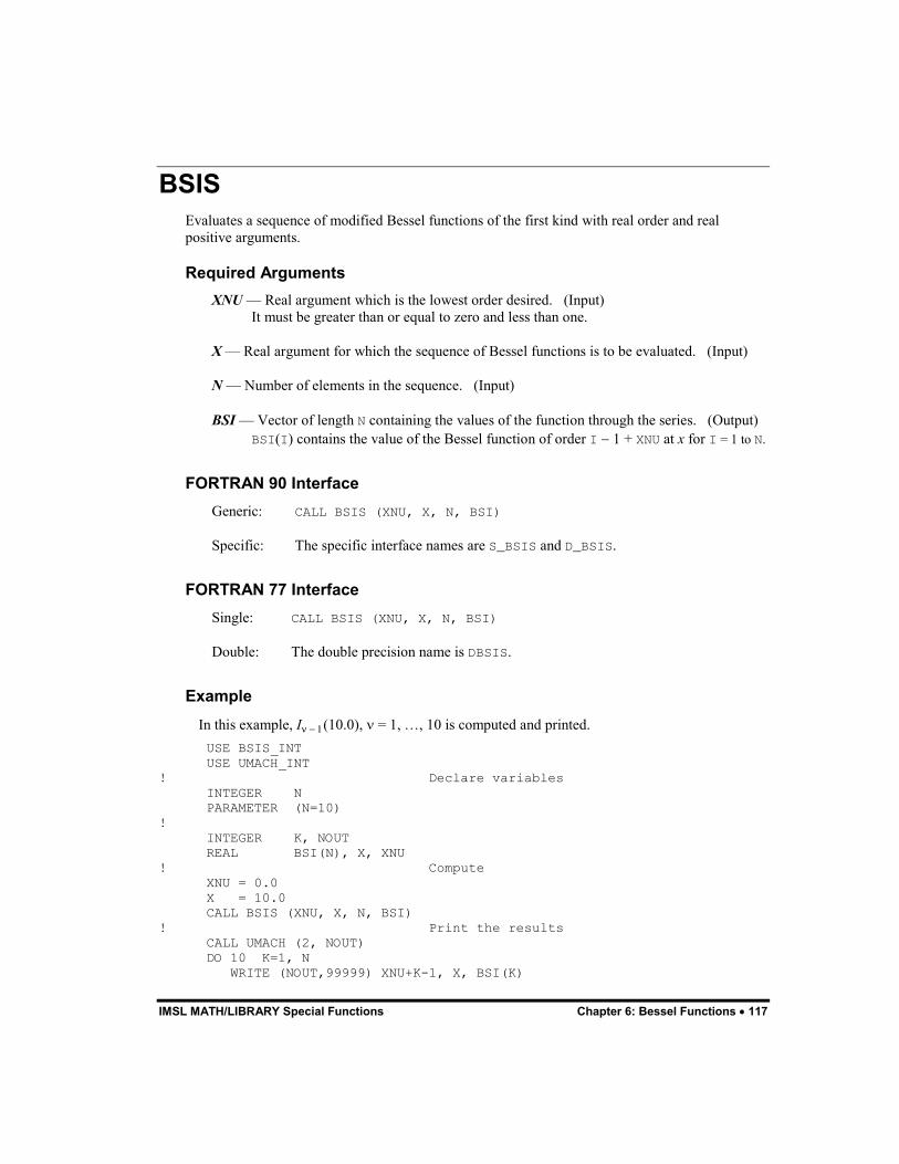
IMSL MATH/LIBRARY Special Functions Chapter 6: Bessel Functions � 117
BSIS Evaluates a sequence of modified Bessel functions of the first kind with real order and real positive arguments.
Required Arguments XNU � Real argument which is the lowest order desired. (Input)
It must be greater than or equal to zero and less than one.
X � Real argument for which the sequence of Bessel functions is to be evaluated. (Input)
N � Number of elements in the sequence. (Input)
BSI � Vector of length N containing the values of the function through the series. (Output) BSI(I) contains the value of the Bessel function of order I � 1 + XNU at x for I = 1 to N.
FORTRAN 90 Interface Generic: CALL BSIS (XNU, X, N, BSI)
Specific: The specific interface names are S_BSIS and D_BSIS.
FORTRAN 77 Interface Single: CALL BSIS (XNU, X, N, BSI)
Double: The double precision name is DBSIS.
Example In this example, I� �(10.0), � = 1, �, 10 is computed and printed.
USE BSIS_INT USE UMACH_INT ! Declare variables INTEGER N PARAMETER (N=10) ! INTEGER K, NOUT REAL BSI(N), X, XNU ! Compute XNU = 0.0 X = 10.0 CALL BSIS (XNU, X, N, BSI) ! Print the results CALL UMACH (2, NOUT) DO 10 K=1, N WRITE (NOUT,99999) XNU+K-1, X, BSI(K)
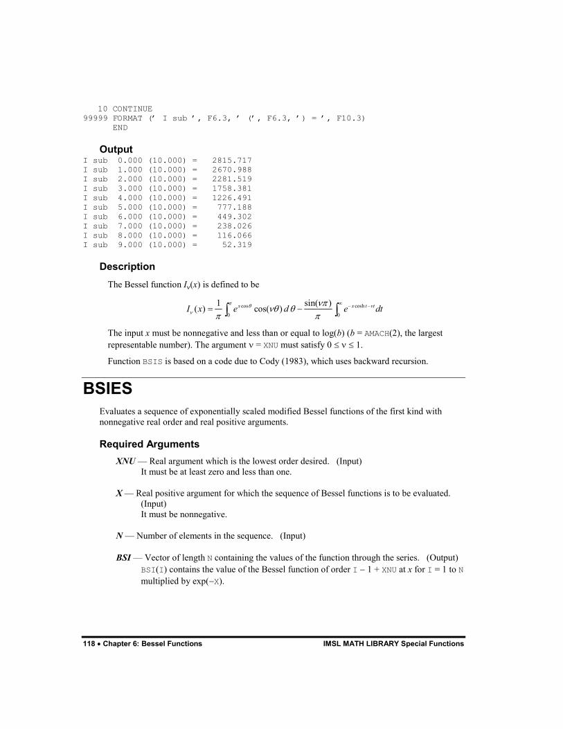
118 � Chapter 6: Bessel Functions IMSL MATH LIBRARY Special Functions
10 CONTINUE 99999 FORMAT (� I sub �, F6.3, � (�, F6.3, �) = �, F10.3) END
Output I sub 0.000 (10.000) = 2815.717 I sub 1.000 (10.000) = 2670.988 I sub 2.000 (10.000) = 2281.519 I sub 3.000 (10.000) = 1758.381 I sub 4.000 (10.000) = 1226.491 I sub 5.000 (10.000) = 777.188 I sub 6.000 (10.000) = 449.302 I sub 7.000 (10.000) = 238.026 I sub 8.000 (10.000) = 116.066 I sub 9.000 (10.000) = 52.319
Description The Bessel function I�(x) is defined to be
cos cosh
0 0
1 sin( )( ) cos( )x x t vtI x e d e dt�
�
�
���� �
� �
�� �
� �� �
The input x must be nonnegative and less than or equal to log(b) (b = AMACH(2), the largest representable number). The argument � = XNU must satisfy 0 � � � 1.
Function BSIS is based on a code due to Cody (1983), which uses backward recursion.
BSIES Evaluates a sequence of exponentially scaled modified Bessel functions of the first kind with nonnegative real order and real positive arguments.
Required Arguments XNU � Real argument which is the lowest order desired. (Input)
It must be at least zero and less than one.
X � Real positive argument for which the sequence of Bessel functions is to be evaluated. (Input) It must be nonnegative.
N � Number of elements in the sequence. (Input)
BSI � Vector of length N containing the values of the function through the series. (Output) BSI(I) contains the value of the Bessel function of order I � 1 + XNU at x for I = 1 to N multiplied by exp(�X).
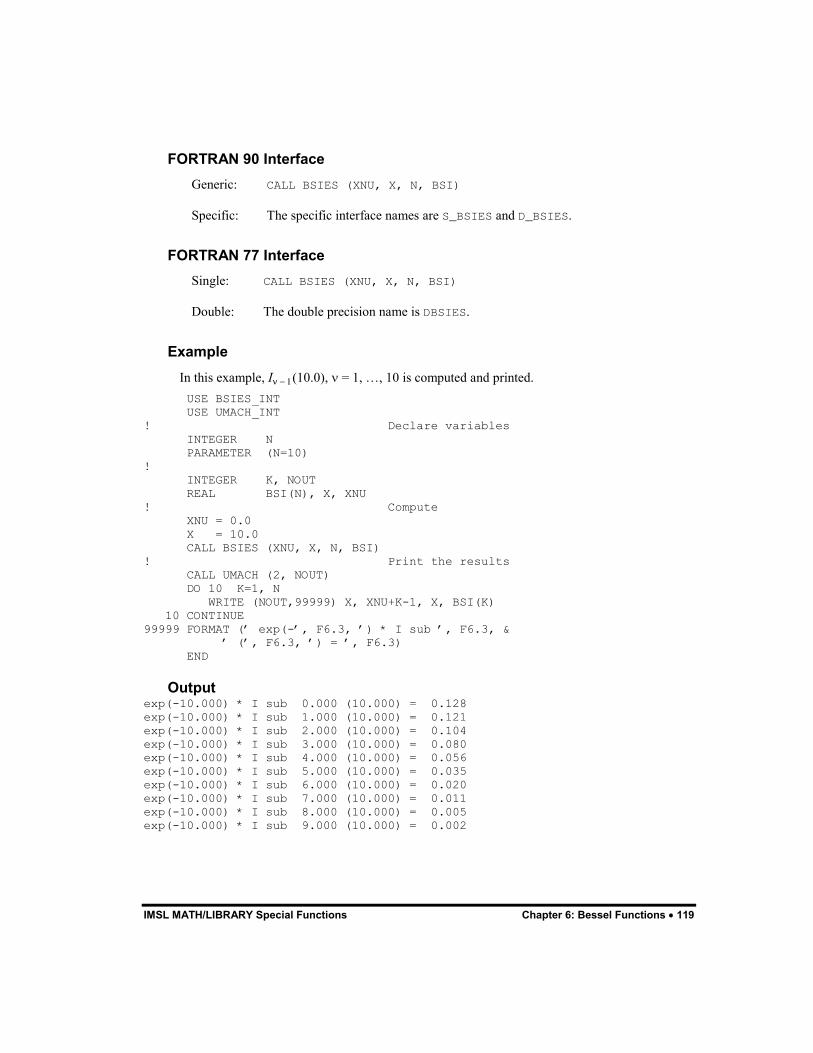
IMSL MATH/LIBRARY Special Functions Chapter 6: Bessel Functions � 119
FORTRAN 90 Interface Generic: CALL BSIES (XNU, X, N, BSI)
Specific: The specific interface names are S_BSIES and D_BSIES.
FORTRAN 77 Interface Single: CALL BSIES (XNU, X, N, BSI)
Double: The double precision name is DBSIES.
Example In this example, I� �(10.0), � = 1, �, 10 is computed and printed.
USE BSIES_INT USE UMACH_INT ! Declare variables INTEGER N PARAMETER (N=10) ! INTEGER K, NOUT REAL BSI(N), X, XNU ! Compute XNU = 0.0 X = 10.0 CALL BSIES (XNU, X, N, BSI) ! Print the results CALL UMACH (2, NOUT) DO 10 K=1, N WRITE (NOUT,99999) X, XNU+K-1, X, BSI(K) 10 CONTINUE 99999 FORMAT (� exp(-�, F6.3, �) * I sub �, F6.3, & � (�, F6.3, �) = �, F6.3) END
Output exp(-10.000) * I sub 0.000 (10.000) = 0.128 exp(-10.000) * I sub 1.000 (10.000) = 0.121 exp(-10.000) * I sub 2.000 (10.000) = 0.104 exp(-10.000) * I sub 3.000 (10.000) = 0.080 exp(-10.000) * I sub 4.000 (10.000) = 0.056 exp(-10.000) * I sub 5.000 (10.000) = 0.035 exp(-10.000) * I sub 6.000 (10.000) = 0.020 exp(-10.000) * I sub 7.000 (10.000) = 0.011 exp(-10.000) * I sub 8.000 (10.000) = 0.005 exp(-10.000) * I sub 9.000 (10.000) = 0.002
120 � Chapter 6: Bessel Functions IMSL MATH LIBRARY Special Functions
Description
Function BSIES evaluates e�x I� � k �(x), for k = 1, �, n. For the definition of I�(x), see BSIS (page 117). The algorithm is based on a code due to Cody (1983), which uses backward recursion.
BSKS Evaluates a sequence of modified Bessel functions of the second kind of fractional order.
Required Arguments XNU � Fractional order of the function. (Input)
XNU must be less than one in absolute value.
X � Argument for which the sequence of Bessel functions is to be evaluated. (Input)
NIN � Number of elements in the sequence. (Input)
BK � Vector of length NIN containing the values of the function through the series. (Output)
FORTRAN 90 Interface Generic: CALL BSKS (XNU, X, NIN, BK)
Specific: The specific interface names are S_BSKS and D_BSKS.
FORTRAN 77 Interface Single: CALL BSKS (XNU, X, NIN, BK)
Double: The double precision name is DBSKS.
Example In this example, K��(10.0), � = 1, �, 10 is computed and printed.
USE BSKS_INT USE UMACH_INT ! Declare variables INTEGER NIN PARAMETER (NIN=10) ! INTEGER K, NOUT REAL BS(NIN), X, XNU ! Compute XNU = 0.0 X = 10.0
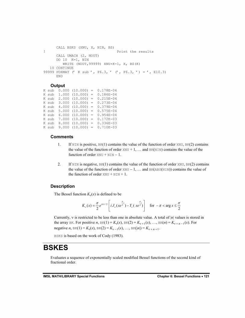
IMSL MATH/LIBRARY Special Functions Chapter 6: Bessel Functions � 121
CALL BSKS (XNU, X, NIN, BS) ! Print the results CALL UMACH (2, NOUT) DO 10 K=1, NIN WRITE (NOUT,99999) XNU+K-1, X, BS(K) 10 CONTINUE 99999 FORMAT (� K sub �, F6.3, � (�, F6.3, �) = �, E10.3) END
Output K sub 0.000 (10.000) = 0.178E-04 K sub 1.000 (10.000) = 0.186E-04 K sub 2.000 (10.000) = 0.215E-04 K sub 3.000 (10.000) = 0.273E-04 K sub 4.000 (10.000) = 0.379E-04 K sub 5.000 (10.000) = 0.575E-04 K sub 6.000 (10.000) = 0.954E-04 K sub 7.000 (10.000) = 0.172E-03 K sub 8.000 (10.000) = 0.336E-03 K sub 9.000 (10.000) = 0.710E-03
Comments 1. If NIN is positive, BK(1) contains the value of the function of order XNU, BK(2) contains
the value of the function of order XNU + 1, � and BK(NIN) contains the value of the function of order XNU + NIN � 1.
2. If NIN is negative, BK(1) contains the value of the function of order XNU, BK(2) contains the value of the function of order XNU � 1, � and BK(ABS(NIN)) contains the value of the function of order XNU + NIN + 1.
Description The Bessel function K�(x) is defined to be
/ 2 2 2( ) ( ) ( ) for arg2 2
i iiK x e i J xe Y xe x� �
��
� � �
� �
�
� �� � � � �� �
Currently, � is restricted to be less than one in absolute value. A total of |n| values is stored in the array BK. For positive n, BK(1) = K�(x), BK(2) = K� � �(x), �, BK(n) = K� � n �(x). For negative n, BK(1) = K�(x), BK(2) = K� �(x), �, BK(|n|) = K� � n � �.
BSKS is based on the work of Cody (1983).
BSKES Evaluates a sequence of exponentially scaled modified Bessel functions of the second kind of fractional order.
122 � Chapter 6: Bessel Functions IMSL MATH LIBRARY Special Functions
Required Arguments XNU � Fractional order of the function. (Input)
XNU must be less than 1.0 in absolute value.
X � Argument for which the sequence of Bessel functions is to be evaluated. (Input)
NIN � Number of elements in the sequence. (Input)
BKE � Vector of length NIN containing the values of the function through the series. (Output)
FORTRAN 90 Interface Generic: CALL BSKES (XNU, X, NIN, BKE)
Specific: The specific interface names are S_BSKES and D_BSKES.
FORTRAN 77 Interface Single: CALL BSKES (XNU, X, NIN, BKE)
Double: The double precision name is DBSKES.
Example In this example, K� �/�(2.0), � = 1, �, 6 is computed and printed.
USE BSKES_INT USE UMACH_INT ! Declare variables INTEGER NIN PARAMETER (NIN=6) ! INTEGER K, NOUT REAL BKE(NIN), X, XNU ! Compute XNU = 0.5 X = 2.0 CALL BSKES (XNU, X, NIN, BKE) ! Print the results CALL UMACH (2, NOUT) DO 10 K=1, NIN WRITE (NOUT,99999) X, XNU+K-1, X, BKE(K) 10 CONTINUE 99999 FORMAT (� exp(�, F6.3, �) * K sub �, F6.3, & � (�, F6.3, �) = �, F8.3) END
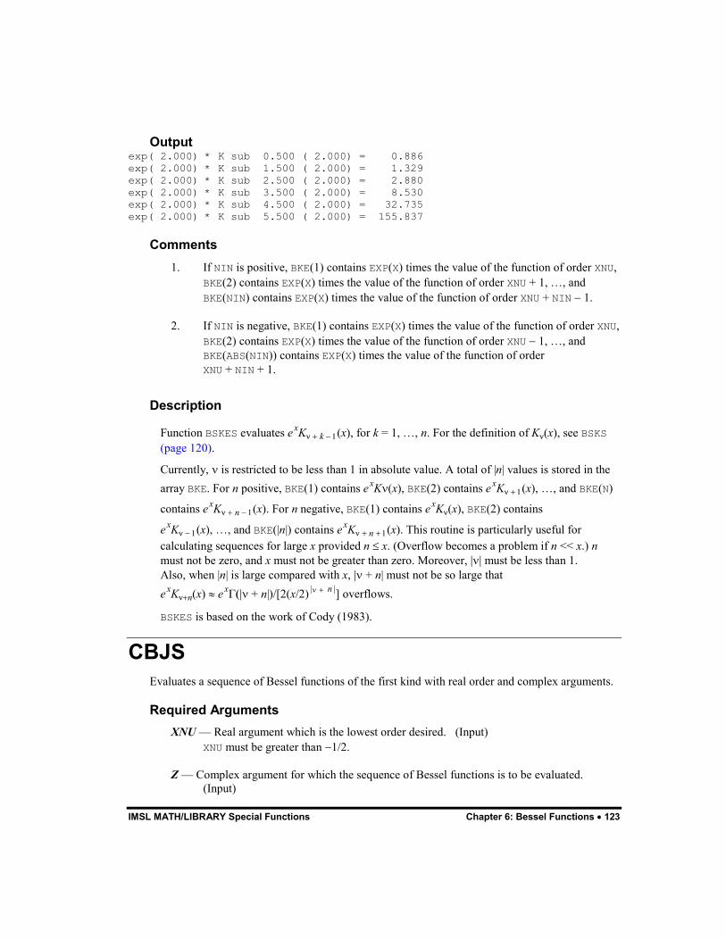
IMSL MATH/LIBRARY Special Functions Chapter 6: Bessel Functions � 123
Output exp( 2.000) * K sub 0.500 ( 2.000) = 0.886 exp( 2.000) * K sub 1.500 ( 2.000) = 1.329 exp( 2.000) * K sub 2.500 ( 2.000) = 2.880 exp( 2.000) * K sub 3.500 ( 2.000) = 8.530 exp( 2.000) * K sub 4.500 ( 2.000) = 32.735 exp( 2.000) * K sub 5.500 ( 2.000) = 155.837
Comments 1. If NIN is positive, BKE(1) contains EXP(X) times the value of the function of order XNU,
BKE(2) contains EXP(X) times the value of the function of order XNU + 1, �, and BKE(NIN) contains EXP(X) times the value of the function of order XNU + NIN � 1.
2. If NIN is negative, BKE(1) contains EXP(X) times the value of the function of order XNU, BKE(2) contains EXP(X) times the value of the function of order XNU � 1, �, and BKE(ABS(NIN)) contains EXP(X) times the value of the function of order XNU + NIN + 1.
Description
Function BSKES evaluates exK� � k �(x), for k = 1, �, n. For the definition of K�(x), see BSKS (page 120).
Currently, � is restricted to be less than 1 in absolute value. A total of |n| values is stored in the array BKE. For n positive, BKE(1) contains exK�(x), BKE(2) contains exK� � �(x), �, and BKE(N)
contains exK� � n �(x). For n negative, BKE(1) contains exK�(x), BKE(2) contains
exK� �(x), �, and BKE(|n|) contains exK� � n � �(x). This routine is particularly useful for calculating sequences for large x provided n � x. (Overflow becomes a problem if n << x.) n must not be zero, and x must not be greater than zero. Moreover, ��� must be less than 1. Also, when |n| is large compared with x, �� + n| must not be so large that exK��n(x) � ex�� + n|)/[2(x/2)|� � n|] overflows.
BSKES is based on the work of Cody (1983).
CBJS Evaluates a sequence of Bessel functions of the first kind with real order and complex arguments.
Required Arguments XNU � Real argument which is the lowest order desired. (Input)
XNU must be greater than �1/2.
Z � Complex argument for which the sequence of Bessel functions is to be evaluated. (Input)
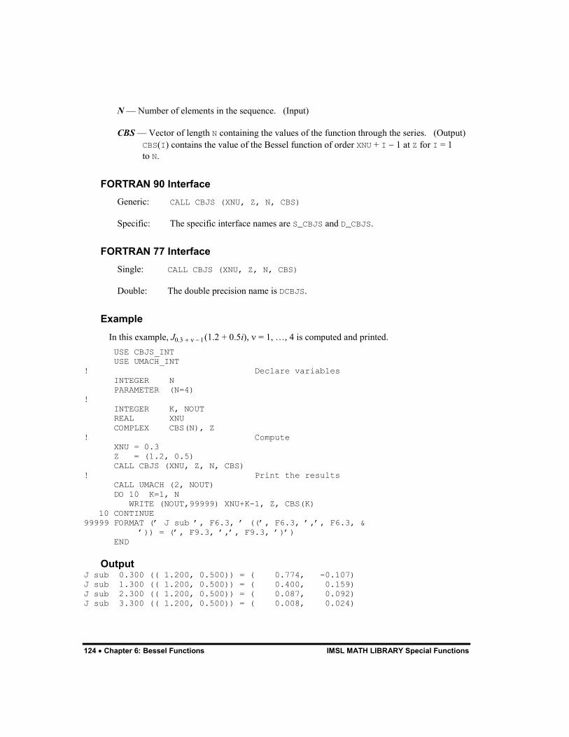
124 � Chapter 6: Bessel Functions IMSL MATH LIBRARY Special Functions
N � Number of elements in the sequence. (Input)
CBS � Vector of length N containing the values of the function through the series. (Output) CBS(I) contains the value of the Bessel function of order XNU + I � 1 at Z for I = 1 to N.
FORTRAN 90 Interface Generic: CALL CBJS (XNU, Z, N, CBS)
Specific: The specific interface names are S_CBJS and D_CBJS.
FORTRAN 77 Interface Single: CALL CBJS (XNU, Z, N, CBS)
Double: The double precision name is DCBJS.
Example In this example, J�. � � �(1.2 + 0.5i), � = 1, �, 4 is computed and printed.
USE CBJS_INT USE UMACH_INT ! Declare variables INTEGER N PARAMETER (N=4) ! INTEGER K, NOUT REAL XNU COMPLEX CBS(N), Z ! Compute XNU = 0.3 Z = (1.2, 0.5) CALL CBJS (XNU, Z, N, CBS) ! Print the results CALL UMACH (2, NOUT) DO 10 K=1, N WRITE (NOUT,99999) XNU+K-1, Z, CBS(K) 10 CONTINUE 99999 FORMAT (� J sub �, F6.3, � ((�, F6.3, �,�, F6.3, & �)) = (�, F9.3, �,�, F9.3, �)�) END
Output J sub 0.300 (( 1.200, 0.500)) = ( 0.774, -0.107) J sub 1.300 (( 1.200, 0.500)) = ( 0.400, 0.159) J sub 2.300 (( 1.200, 0.500)) = ( 0.087, 0.092) J sub 3.300 (( 1.200, 0.500)) = ( 0.008, 0.024)
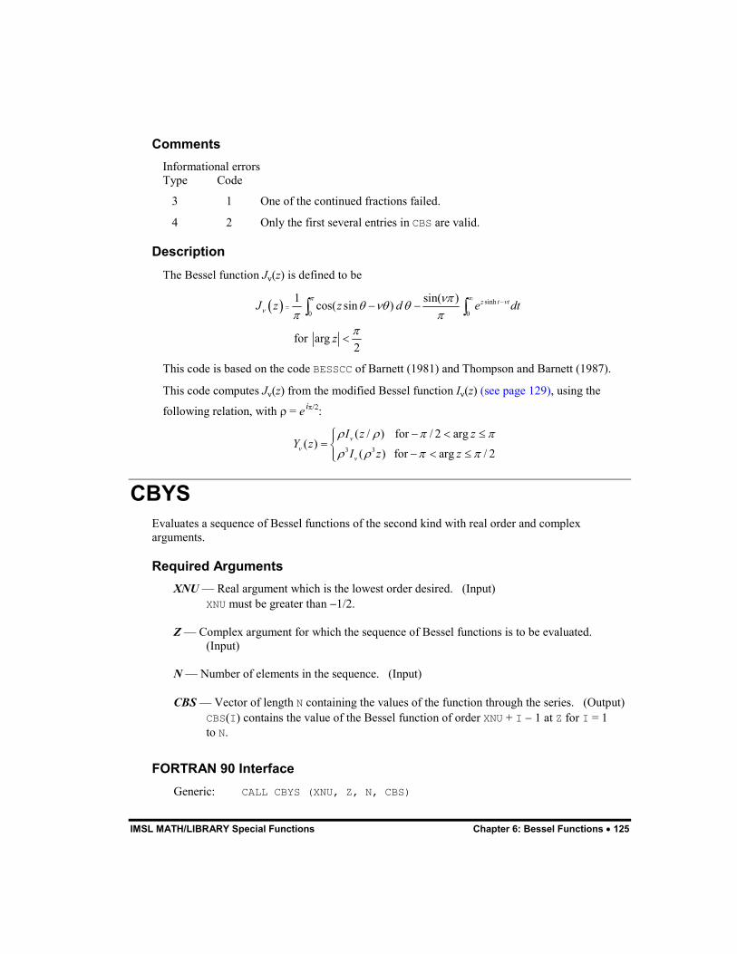
IMSL MATH/LIBRARY Special Functions Chapter 6: Bessel Functions � 125
Comments Informational errors Type Code
3 1 One of the continued fractions failed.
4 2 Only the first several entries in CBS are valid.
Description The Bessel function J�(z) is defined to be
� � sinh
0 0
1 sin( )cos( sin )
for arg2
z t vtJ z z d e dt
z
�
�
��� �� �
� �
�
��
� � �
�
� �
This code is based on the code BESSCC of Barnett (1981) and Thompson and Barnett (1987).
This code computes J�(z) from the modified Bessel function I�(z) (see page 129), using the
following relation, with � = ei�:
3 3
( / ) for / 2 arg( )
( ) for arg / 2v
vv
I z zY z
I z z
� � � �
� � � �
� � ���� �
� � ���
CBYS Evaluates a sequence of Bessel functions of the second kind with real order and complex arguments.
Required Arguments XNU � Real argument which is the lowest order desired. (Input)
XNU must be greater than �1/2.
Z � Complex argument for which the sequence of Bessel functions is to be evaluated. (Input)
N � Number of elements in the sequence. (Input)
CBS � Vector of length N containing the values of the function through the series. (Output) CBS(I) contains the value of the Bessel function of order XNU + I � 1 at Z for I = 1 to N.
FORTRAN 90 Interface Generic: CALL CBYS (XNU, Z, N, CBS)
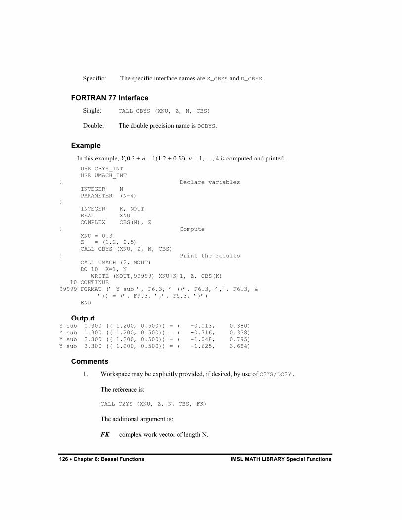
126 � Chapter 6: Bessel Functions IMSL MATH LIBRARY Special Functions
Specific: The specific interface names are S_CBYS and D_CBYS.
FORTRAN 77 Interface Single: CALL CBYS (XNU, Z, N, CBS)
Double: The double precision name is DCBYS.
Example In this example, Y�0.3 + n � 1(1.2 + 0.5i), � = 1, �, 4 is computed and printed.
USE CBYS_INT USE UMACH_INT ! Declare variables INTEGER N PARAMETER (N=4) ! INTEGER K, NOUT REAL XNU COMPLEX CBS(N), Z ! Compute XNU = 0.3 Z = (1.2, 0.5) CALL CBYS (XNU, Z, N, CBS) ! Print the results CALL UMACH (2, NOUT) DO 10 K=1, N WRITE (NOUT,99999) XNU+K-1, Z, CBS(K) 10 CONTINUE 99999 FORMAT (� Y sub �, F6.3, � ((�, F6.3, �,�, F6.3, & �)) = (�, F9.3, �,�, F9.3, �)�) END
Output Y sub 0.300 (( 1.200, 0.500)) = ( -0.013, 0.380) Y sub 1.300 (( 1.200, 0.500)) = ( -0.716, 0.338) Y sub 2.300 (( 1.200, 0.500)) = ( -1.048, 0.795) Y sub 3.300 (( 1.200, 0.500)) = ( -1.625, 3.684)
Comments 1. Workspace may be explicitly provided, if desired, by use of C2YS/DC2Y.
The reference is:
CALL C2YS (XNU, Z, N, CBS, FK)
The additional argument is:
FK � complex work vector of length N.
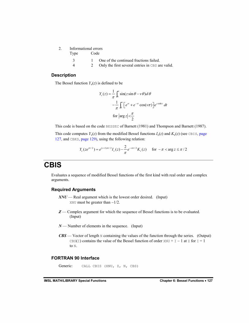
IMSL MATH/LIBRARY Special Functions Chapter 6: Bessel Functions � 127
2. Informational errors Type Code
3 1 One of the continued fractions failed. 4 2 Only the first several entries in CBS are valid.
Description The Bessel function Y�(z) is defined to be
0
sinh
0
1( ) sin( sin )
1 cos( )
for arg2
v
vt vt z t
Y z z v d
e e v e dt
z
�
� � ��
��
�
��
� �
� �� �� �
�
�
�
This code is based on the code BESSEC of Barnett (1981) and Thompson and Barnett (1987).
This code computes Y�(z) from the modified Bessel functions I�(z) and K�(z) (see CBIS, page 127, and CBKS, page 129), using the following relation:
/ 2 ( 1) / 2 / 22( ) ( ) ( ) for arg / 2i v i v ivY ze e I z e K z z� � �
� �� �
�
� �
� � � � �
CBIS Evaluates a sequence of modified Bessel functions of the first kind with real order and complex arguments.
Required Arguments XNU � Real argument which is the lowest order desired. (Input)
XNU must be greater than �1/2.
Z � Complex argument for which the sequence of Bessel functions is to be evaluated. (Input)
N � Number of elements in the sequence. (Input)
CBS � Vector of length N containing the values of the function through the series. (Output) CBS(I) contains the value of the Bessel function of order XNU + I � 1 at Z for I = 1 to N.
FORTRAN 90 Interface Generic: CALL CBIS (XNU, Z, N, CBS)
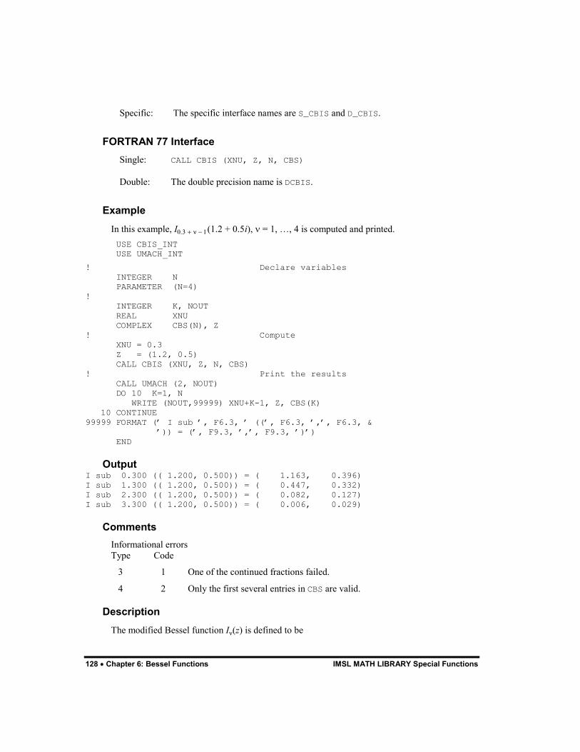
128 � Chapter 6: Bessel Functions IMSL MATH LIBRARY Special Functions
Specific: The specific interface names are S_CBIS and D_CBIS.
FORTRAN 77 Interface Single: CALL CBIS (XNU, Z, N, CBS)
Double: The double precision name is DCBIS.
Example In this example, I�. � � �(1.2 + 0.5i), � = 1, �, 4 is computed and printed.
USE CBIS_INT USE UMACH_INT
! Declare variables INTEGER N PARAMETER (N=4) ! INTEGER K, NOUT REAL XNU COMPLEX CBS(N), Z ! Compute XNU = 0.3 Z = (1.2, 0.5) CALL CBIS (XNU, Z, N, CBS) ! Print the results CALL UMACH (2, NOUT) DO 10 K=1, N WRITE (NOUT,99999) XNU+K-1, Z, CBS(K) 10 CONTINUE 99999 FORMAT (� I sub �, F6.3, � ((�, F6.3, �,�, F6.3, & �)) = (�, F9.3, �,�, F9.3, �)�) END
Output I sub 0.300 (( 1.200, 0.500)) = ( 1.163, 0.396) I sub 1.300 (( 1.200, 0.500)) = ( 0.447, 0.332) I sub 2.300 (( 1.200, 0.500)) = ( 0.082, 0.127) I sub 3.300 (( 1.200, 0.500)) = ( 0.006, 0.029)
Comments Informational errors Type Code
3 1 One of the continued fractions failed.
4 2 Only the first several entries in CBS are valid.
Description The modified Bessel function I�(z) is defined to be
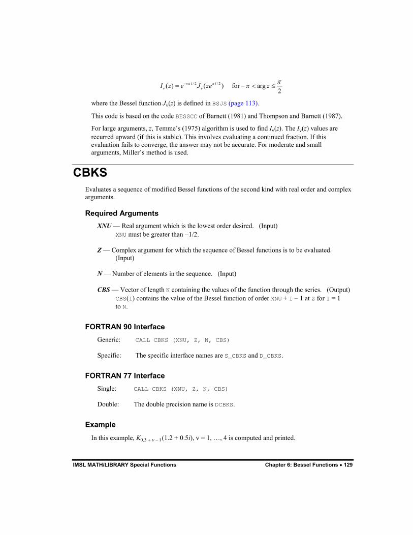
IMSL MATH/LIBRARY Special Functions Chapter 6: Bessel Functions � 129
/ 2 / 2( ) ( ) for arg2
v i iv vI z e J ze z� �
�
��
� � � �
where the Bessel function J�(z) is defined in BSJS (page 113).
This code is based on the code BESSCC of Barnett (1981) and Thompson and Barnett (1987).
For large arguments, z, Temme�s (1975) algorithm is used to find I�(z). The I�(z) values are recurred upward (if this is stable). This involves evaluating a continued fraction. If this evaluation fails to converge, the answer may not be accurate. For moderate and small arguments, Miller�s method is used.
CBKS Evaluates a sequence of modified Bessel functions of the second kind with real order and complex arguments.
Required Arguments XNU � Real argument which is the lowest order desired. (Input)
XNU must be greater than �1/2.
Z � Complex argument for which the sequence of Bessel functions is to be evaluated. (Input)
N � Number of elements in the sequence. (Input)
CBS � Vector of length N containing the values of the function through the series. (Output) CBS(I) contains the value of the Bessel function of order XNU + I � 1 at Z for I = 1 to N.
FORTRAN 90 Interface Generic: CALL CBKS (XNU, Z, N, CBS)
Specific: The specific interface names are S_CBKS and D_CBKS.
FORTRAN 77 Interface Single: CALL CBKS (XNU, Z, N, CBS)
Double: The double precision name is DCBKS.
Example In this example, K�. � v �(1.2 + 0.5i), � = 1, �, 4 is computed and printed.
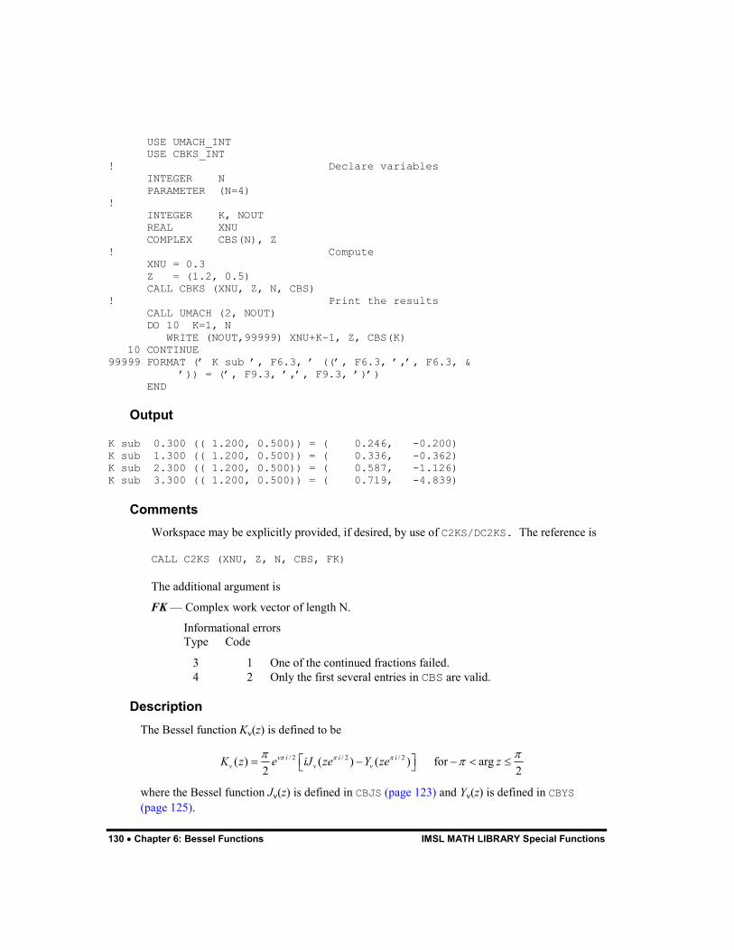
130 � Chapter 6: Bessel Functions IMSL MATH LIBRARY Special Functions
USE UMACH_INT USE CBKS_INT ! Declare variables INTEGER N PARAMETER (N=4) ! INTEGER K, NOUT REAL XNU COMPLEX CBS(N), Z ! Compute XNU = 0.3 Z = (1.2, 0.5) CALL CBKS (XNU, Z, N, CBS) ! Print the results CALL UMACH (2, NOUT) DO 10 K=1, N WRITE (NOUT,99999) XNU+K-1, Z, CBS(K) 10 CONTINUE 99999 FORMAT (� K sub �, F6.3, � ((�, F6.3, �,�, F6.3, & �)) = (�, F9.3, �,�, F9.3, �)�) END
Output
K sub 0.300 (( 1.200, 0.500)) = ( 0.246, -0.200) K sub 1.300 (( 1.200, 0.500)) = ( 0.336, -0.362) K sub 2.300 (( 1.200, 0.500)) = ( 0.587, -1.126) K sub 3.300 (( 1.200, 0.500)) = ( 0.719, -4.839)
Comments Workspace may be explicitly provided, if desired, by use of C2KS/DC2KS. The reference is
CALL C2KS (XNU, Z, N, CBS, FK)
The additional argument is
FK � Complex work vector of length N.
Informational errors Type Code
3 1 One of the continued fractions failed. 4 2 Only the first several entries in CBS are valid.
Description The Bessel function K�(z) is defined to be
/ 2 / 2 / 2( ) ( ) ( ) for arg2 2
v i i iv v vK z e iJ ze Y ze z� � �
� �
�� �� � � � �� �
where the Bessel function J�(z) is defined in CBJS (page 123) and Y�(z) is defined in CBYS (page 125).

IMSL MATH/LIBRARY Special Functions Chapter 6: Bessel Functions � 131
This code is based on the code BESSCC of Barnett (1981) and Thompson and Barnett (1987).
For moderate or large arguments, z, Temme�s (1975) algorithm is used to find K�(z). This involves evaluating a continued fraction. If this evaluation fails to converge, the answer may not be accurate. For small z, a Neumann series is used to compute K�(z). Upward recurrence of the K�(z) is always stable.

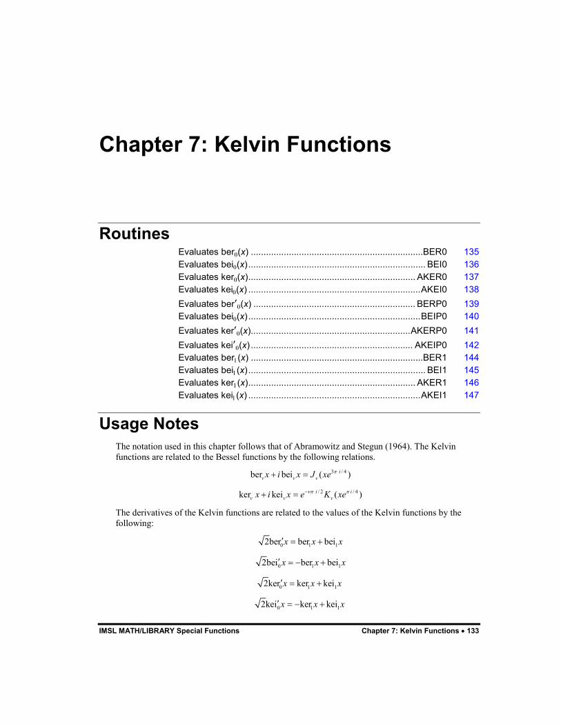
IMSL MATH/LIBRARY Special Functions Chapter 7: Kelvin Functions � 133
Chapter 7: Kelvin Functions
Routines Evaluates ber�(x) ....................................................................BER0 135 Evaluates bei�(x)...................................................................... BEI0 136 Evaluates ker�(x).................................................................. AKER0 137 Evaluates kei�(x) ....................................................................AKEI0 138 Evaluates ber��(x) ................................................................ BERP0 139 Evaluates bei�(x)....................................................................BEIP0 140 Evaluates ker��(x)...............................................................AKERP0 141 Evaluates kei��(x) ................................................................ AKEIP0 142 Evaluates ber�(x) ....................................................................BER1 144 Evaluates bei�(x)...................................................................... BEI1 145 Evaluates ker�(x).................................................................. AKER1 146 Evaluates kei�(x) ....................................................................AKEI1 147
Usage Notes The notation used in this chapter follows that of Abramowitz and Stegun (1964). The Kelvin functions are related to the Bessel functions by the following relations.
3 / 4ber bei ( )iv v vx i x J xe �
� �
/ 2 / 4ker kei ( )i iv v vx i x e K xe�� ��
� �
The derivatives of the Kelvin functions are related to the values of the Kelvin functions by the following:
0 1 12ber ber beix x x� � �
0 1 12bei ber beix x x� � � �
0 1 12ker ker keix x x� � �
0 1 12kei ker keix x x� � � �
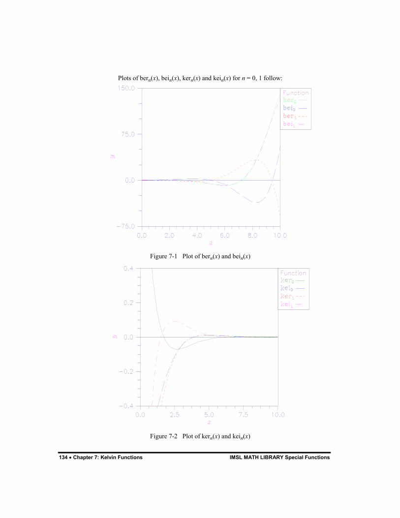
134 � Chapter 7: Kelvin Functions IMSL MATH LIBRARY Special Functions
Plots of bern(x), bein(x), kern(x) and kein(x) for n = 0, 1 follow:
Figure 7-1 Plot of bern(x) and bein(x)
Figure 7-2 Plot of kern(x) and kein(x)
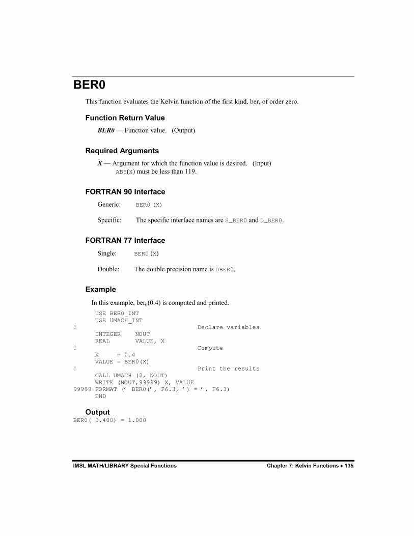
IMSL MATH/LIBRARY Special Functions Chapter 7: Kelvin Functions � 135
BER0 This function evaluates the Kelvin function of the first kind, ber, of order zero.
Function Return Value BER0 � Function value. (Output)
Required Arguments X � Argument for which the function value is desired. (Input)
ABS(X) must be less than 119.
FORTRAN 90 Interface Generic: BER0 (X)
Specific: The specific interface names are S_BER0 and D_BER0.
FORTRAN 77 Interface Single: BER0 (X)
Double: The double precision name is DBER0.
Example In this example, ber�(0.4) is computed and printed.
USE BER0_INT USE UMACH_INT ! Declare variables INTEGER NOUT REAL VALUE, X ! Compute X = 0.4 VALUE = BER0(X) ! Print the results CALL UMACH (2, NOUT) WRITE (NOUT,99999) X, VALUE 99999 FORMAT (� BER0(�, F6.3, �) = �, F6.3) END
Output BER0( 0.400) = 1.000
136 � Chapter 7: Kelvin Functions IMSL MATH LIBRARY Special Functions
Description
The Kelvin function ber�(x) is defined to be �J�(xe��i��). The Bessel function J�(x) is defined in BSJ0 (page 92). Function BER0 is based on the work of Burgoyne (1963).
BEI0 This function evaluates the Kelvin function of the first kind, bei, of order zero.
Function Return Value BEI0 � Function value. (Output)
Required Arguments X � Argument for which the function value is desired. (Input)
ABS(X) must be less than 119.
FORTRAN 90 Interface Generic: BEI0 (X)
Specific: The specific interface names are S_BEI0 and D_BEI0.
FORTRAN 77 Interface Single: BEI0 (X)
Double: The double precision name is DBEI0.
Example In this example, bei�(0.4) is computed and printed.
USE BEI0_INT USE UMACH_INT ! Declare variables INTEGER NOUT REAL VALUE, X ! Compute X = 0.4 VALUE = BEI0(X) ! Print the results CALL UMACH (2, NOUT) WRITE (NOUT,99999) X, VALUE 99999 FORMAT (� BEI0(�, F6.3, �) = �, F6.3) END
IMSL MATH/LIBRARY Special Functions Chapter 7: Kelvin Functions � 137
Output BEI0( 0.400) = 0.040
Description
The Kelvin function bei�(x) is defined to be �J�(xe��i��). The Bessel function J�(x) is defined in BSJ0 (page 92). Function BEI0 is based on the work of Burgoyne (1963).
In BEI0, x must be less than 119.
AKER0 This function evaluates the Kelvin function of the second kind, ker, of order zero.
Function Return Value AKER0 � Function value. (Output)
Required Arguments X � Argument for which the function value is desired. (Input)
It must be nonnegative.
FORTRAN 90 Interface Generic: AKER0(X)
Specific: The specific interface names are S_AKER0 and D_AKER0.
FORTRAN 77 Interface Single: AKER0(X)
Double: The double precision name is DKER0.
Example In this example, ker�(0.4) is computed and printed.
USE AKER0_INT USE UMACH_INT ! Declare variables INTEGER NOUT REAL VALUE, X ! Compute X = 0.4 VALUE = AKER0(X) ! Print the results CALL UMACH (2, NOUT)
138 � Chapter 7: Kelvin Functions IMSL MATH LIBRARY Special Functions
WRITE (NOUT,99999) X, VALUE 99999 FORMAT (� AKER0(�, F6.3, �) = �, F6.3) END
Output AKER0( 0.400) = 1.063
Description
The modified Kelvin function ker�(x) is defined to be �K�(xe�i��). The Bessel function K�(x) is defined in BSK0 (page 101). Function AKER0 is based on the work of Burgoyne (1963). If x < 0, then NaN (not a number) is returned. If x � 119, then zero is returned.
AKEI0 This function evaluates the Kelvin function of the second kind, kei, of order zero.
Function Return Value AKEI0 � Function value. (Output)
Required Arguments X � Argument for which the function value is desired. (Input)
It must be nonnegative and less than 119.
FORTRAN 90 Interface Generic: AKEI0(X)
Specific: The specific interface names are S_AKEI0 and D_AKEI0.
FORTRAN 77 Interface Single: AKEI0(X)
Double: The double precision name is DKEI0.
Example In this example, kei�(0.4) is computed and printed.
USE AKEI0_INT USE UMACH_INT ! Declare variables INTEGER NOUT REAL VALUE, X ! Compute X = 0.4
IMSL MATH/LIBRARY Special Functions Chapter 7: Kelvin Functions � 139
VALUE = AKEI0(X) ! Print the results CALL UMACH (2, NOUT) WRITE (NOUT,99999) X, VALUE 99999 FORMAT (� AKEI0(�, F6.3, �) = �, F6.3) END
Output AKEI0( 0.400) = -0.704
Description
The modified Kelvin function kei�(x) is defined to be �K�(xe�i��). The Bessel function K�(x) is defined in BSK0 (page 101). Function AKEI0 is based on the work of Burgoyne (1963).
In AKEI0, x must satisfy 0 � x < 119. If x < 0, then NaN (not a number) is returned. If x � 119, then zero is returned.
BERP0 This function evaluates the derivative of the Kelvin function of the first kind, ber, of order zero.
Function Return Value BERP0 � Function value. (Output)
Required Arguments X � Argument for which the function value is desired. (Input)
FORTRAN 90 Interface Generic: BERP0 (X)
Specific: The specific interface names are S_BERP0 and D_BERP0.
FORTRAN 77 Interface Single: BERP0 (X)
Double: The double precision name is DBERP0.
Example In this example, ber�0(0.6) is computed and printed.
USE BERP0_INT USE UMACH_INT
140 � Chapter 7: Kelvin Functions IMSL MATH LIBRARY Special Functions
! Declare variables INTEGER NOUT REAL VALUE, X ! Compute X = 0.6 VALUE = BERP0(X) ! Print the results CALL UMACH (2, NOUT) WRITE (NOUT,99999) X, VALUE 99999 FORMAT (� BERP0(�, F6.3, �) = �, F6.3) END
Output BERP0( 0.600) = -0.013
Description The function ber��(x) is defined to be
� �0 berd xdx
where ber�(x) is a Kelvin function, see BER0 (page 135). Function BERP0 is based on the work of Burgoyne (1963).
If �x� > 119, then NaN (not a number) is returned.
BEIP0 This function evaluates the derivative of the Kelvin function of the first kind, bei, of order zero.
Function Return Value BEIP0 � Function value. (Output)
Required Arguments X � Argument for which the function value is desired. (Input)
FORTRAN 90 Interface Generic: BEIP0 (X)
Specific: The specific interface names are S_BEIP0 and D_BEIP0.
FORTRAN 77 Interface Single: BEIP0 (X)
Double: The double precision name is DBEIP0.
IMSL MATH/LIBRARY Special Functions Chapter 7: Kelvin Functions � 141
Example In this example, bei��(0.6) is computed and printed.
USE BEIP0_INT USE UMACH_INT ! Declare variables INTEGER NOUT REAL VALUE, X ! Compute X = 0.6 VALUE = BEIP0(X) ! Print the results CALL UMACH (2, NOUT) WRITE (NOUT,99999) X, VALUE 99999 FORMAT (� BEIP0(�, F6.3, �) = �, F6.3) END
Output BEIP0( 0.600) = 0.300
Description The function bei��(x) is defined to be
� �0 beid xdx
where bei�(x) is a Kelvin function, see BEI0 (page 136). Function BEIP0 is based on the work of Burgoyne (1963).
If |x| > 119, then NaN (not a number) is returned.
AKERP0 This function evaluates the derivative of the Kelvin function of the second kind, ker, of order zero.
Function Return Value AKERP0 � Function value. (Output)
Required Arguments X � Argument for which the function value is desired. (Input)
It must be nonnegative.
FORTRAN 90 Interface Generic: AKERP0 (X)
142 � Chapter 7: Kelvin Functions IMSL MATH LIBRARY Special Functions
Specific: The specific interface names are S_AKERP0 and D_AKERP0.
FORTRAN 77 Interface Single: AKERP0 (X)
Double: The double precision name is DKERP0.
Example In this example, ker��(0.6) is computed and printed.
USE AKERP0_INT USE UMACH_INT ! Declare variables INTEGER NOUT REAL VALUE, X ! Compute X = 0.6 VALUE = AKERP0(X) ! Print the results CALL UMACH (2, NOUT) WRITE (NOUT,99999) X, VALUE 99999 FORMAT (� AKERP0(�, F6.3, �) = �, F6.3) END
Output AKERP0( 0.600) = -1.457
Description The function ker��(x) is defined to be
� �0 kerd xdx
where ker�(x) is a Kelvin function, see AKER0 (page 137). Function AKERP0 is based on the work of Burgoyne (1963). If x < 0, then NaN (not a number) is returned. If x > 119, then zero is returned.
AKEIP0 This function evaluates the Kelvin function of the second kind, kei, of order zero.
Function Return Value AKEIP0 � Function value. (Output)
IMSL MATH/LIBRARY Special Functions Chapter 7: Kelvin Functions � 143
Required Arguments X � Argument for which the function value is desired. (Input)
It must be nonnegative.
FORTRAN 90 Interface Generic: AKEIP0 (X)
Specific: The specific interface names are S_AKEIP0 and D_AKEIP0.
FORTRAN 77 Interface Single: AKEIP0 (X)
Double: The double precision name is DKEIP0.
Example In this example, kei��(0.6) is computed and printed.
USE AKEIP0_INT USE UMACH_INT ! Declare variables INTEGER NOUT REAL VALUE, X ! Compute X = 0.6 VALUE = AKEIP0(X) ! Print the results CALL UMACH (2, NOUT) WRITE (NOUT,99999) X, VALUE 99999 FORMAT (� AKEIP0(�, F6.3, �) = �, F6.3) END
Output AKEIP0( 0.600) = 0.348
Description The function kei��(x) is defined to be
� �0 keid xdx
where kei�(x) is a Kelvin function, see AKEIP0 (page 142). Function AKEIP0 is based on the work of Burgoyne (1963).
If x < 0, then NaN (not a number) is returned. If x > 119, then zero is returned.
144 � Chapter 7: Kelvin Functions IMSL MATH LIBRARY Special Functions
BER1 This function evaluates the Kelvin function of the first kind, ber, of order one.
Function Return Value BER1 � Function value. (Output)
Required Arguments X � Argument for which the function value is desired. (Input)
FORTRAN 90 Interface Generic: BER1 (X)
Specific: The specific interface names are S_BER1 and D_BER1.
FORTRAN 77 Interface Single: BER1 (X)
Double: The double precision name is DBER1.
Example In this example, ber�(0.4) is computed and printed.
USE BER1_INT USE UMACH_INT ! Declare variables INTEGER NOUT REAL VALUE, X ! Compute X = 0.4 VALUE = BER1(X) ! Print the results CALL UMACH (2, NOUT) WRITE (NOUT,99999) X, VALUE 99999 FORMAT (� BER1(�, F6.3, �) = �, F6.3) END
Output BER1( 0.400) = -0.144
Description
The Kelvin function ber�(x) is defined to be �J�(xe��i��). The Bessel function J�(x) is defined in BSJ1 (page 94). Function BER1 is based on the work of Burgoyne (1963).
IMSL MATH/LIBRARY Special Functions Chapter 7: Kelvin Functions � 145
If |x| > 119, then NaN (not a number) is returned.
BEI1 This function evaluates the Kelvin function of the first kind, bei, of order one.
Function Return Value BEI1 � Function value. (Output)
Required Arguments X � Argument for which the function value is desired. (Input)
FORTRAN 90 Interface Generic: BEI1 (X)
Specific: The specific interface names are S_BEI1 and D_BEI1.
FORTRAN 77 Interface Single: BEI1 (X)
Double: The double precision name is DBEI1.
Example In this example, bei�(0.4) is computed and printed.
USE BEI1_INT USE UMACH_INT ! Declare variables INTEGER NOUT REAL VALUE, X ! Compute X = 0.4 VALUE = BEI1(X) ! Print the results CALL UMACH (2, NOUT) WRITE (NOUT,99999) X, VALUE 99999 FORMAT (� BEI1(�, F6.3, �) = �, F6.3) END
Output BEI1( 0.400) = 0.139
146 � Chapter 7: Kelvin Functions IMSL MATH LIBRARY Special Functions
Description
The Kelvin function bei�(x) is defined to be �J�(xe��i��). The Bessel function J�(x) is defined in BSJ1 (page 94). Function BEI1 is based on the work of Burgoyne (1963).
If |x| > 119, then NaN (not a number) is returned.
AKER1 This function evaluates the Kelvin function of the second kind, ker, of order one.
Function Return Value AKER1 � Function value. (Output)
Required Arguments X � Argument for which the function value is desired. (Input)
It must be nonnegative.
FORTRAN 90 Interface Generic: AKER1 (X)
Specific: The specific interface names are S_AKER1 and D_AKER1.
FORTRAN 77 Interface Single: AKER1 (X)
Double: The double precision name is DKER1.
Example In this example, ker�(0.4) is computed and printed.
USE AKER1_INT USE UMACH_INT ! Declare variables INTEGER NOUT REAL VALUE, X ! Compute X = 0.4 VALUE = AKER1(X) ! Print the results CALL UMACH (2, NOUT) WRITE (NOUT,99999) X, VALUE 99999 FORMAT (� AKER1(�, F6.3, �) = �, F6.3) END
IMSL MATH/LIBRARY Special Functions Chapter 7: Kelvin Functions � 147
Output AKER1( 0.400) = -1.882
Description
The modified Kelvin function ker�(x) is defined to be e��i���K�(xe�i��). The Bessel function K�(x) is defined in BSK1 (page 103). Function AKER1 is based on the work of Burgoyne (1963).
If x < 0, then NaN (not a number) is returned. If x � 119, then zero is returned.
AKEI1 This function evaluates the Kelvin function of the second kind, kei, of order one.
Function Return Value AKEI1 � Function value. (Output)
Required Arguments X � Argument for which the function value is desired. (Input)
It must be nonnegative.
FORTRAN 90 Interface Generic: AKEI1 (X)
Specific: The specific interface names are S_AKEI1 and D_AKEI1.
FORTRAN 77 Interface Single: AKEI1 (X)
Double: The double precision name is DKEI1.
Example In this example, kei�(0.4) is computed and printed.
USE UMACH_INT USE AKEI1_INT
! Declare variables INTEGER NOUT REAL VALUE, X ! Compute X = 0.4 VALUE = AKEI1(X) ! Print the results
148 � Chapter 7: Kelvin Functions IMSL MATH LIBRARY Special Functions
CALL UMACH (2, NOUT) WRITE (NOUT,99999) X, VALUE 99999 FORMAT (� AKEI1(�, F6.3, �) = �, F6.3) END
Output
AKEI1( 0.400) = -1.444
Description
The modified Kelvin function kei�(x) is defined to be e��i���K�(xe�i��). The Bessel function K�(x) is defined in BSK1 (page 103). Function AKER1 is based on the work of Burgoyne (1963).
If x < 0, then NaN (not a number) is returned. If x � 119, then zero is returned.
IMSL MATH/LIBRARY Special Functions Chapter 8: Airy Functions � 149
Chapter 8: Airy Functions
Routines Evaluates Ai(x)..............................................................................AI 149 Evaluates Bi(x)..............................................................................BI 150 Evaluates Ai�(x)..........................................................................AID 152 Evaluates Bi�(x)..........................................................................BID 153 Evaluates exponentially scaled Ai(x) ......................................... AIE 154 Evaluates exponentially scaled Bi(x) ......................................... BIE 155 Evaluates exponentially scaled Ai�(x) ......................................AIDE 157 Evaluates exponentially scaled Bi�(x) ......................................BIDE 158
AI This function evaluates the Airy function.
Function Return Value AI � Function value. (Output)
Required Arguments X � Argument for which the Airy function is desired. (Input)
FORTRAN 90 Interface Generic: AI (X)
Specific: The specific interface names are S_AI and D_AI.
FORTRAN 77 Interface Single: AI (X)
Double: The double precision name is DAI.
150 � Chapter 8: Airy Functions IMSL MATH LIBRARY Special Functions
Example In this example, Ai(�4.9) is computed and printed.
USE AI_INT USE UMACH_INT ! Declare variables INTEGER NOUT REAL VALUE, X ! Compute X = -4.9 VALUE = AI(X) ! Print the results CALL UMACH (2, NOUT) WRITE (NOUT,99999) X, VALUE 99999 FORMAT (� AI(�, F6.3, �) = �, F6.3) END
Output AI(-4.900) = 0.375
Comments Informational error Type Code
2 1 The function underflows because X is greater than XMAX, where XMAX = (�3/2 ln(AMACH(1)))���.
Description The Airy function Ai(x) is defined to be
� � 3 3 / 21/ 320
1 1 2Ai cos3 33
xx xt t dt K x� �
� � � � �� � �� � � �
� � � ��
The Bessel function K�(x) is defined in BSKS (page 120).
If x < �1.31�����, then the answer will have no precision. If x < �1.31�����, the answer will be less accurate than half precision. Here, � = AMACH(4) is the machine precision. Finally, x should be less than x� so the answer does not underflow. Very approximately, x� = {�1.5 ln s}���, where s = AMACH(1), the smallest representable positive number. If underflows are a problem for large x, then the exponentially scaled routine AIE (page 154) should be used.
BI This function evaluates the Airy function of the second kind.
Function Return Value BI � Function value. (Output)
IMSL MATH/LIBRARY Special Functions Chapter 8: Airy Functions � 151
Required Arguments X � Argument for which the Airy function value is desired. (Input)
FORTRAN 90 Interface Generic: BI (X)
Specific: The specific interface names are S_BI and D_BI.
FORTRAN 77 Interface Single: BI (X)
Double: The double precision name is DBI.
Example In this example, Bi(�4.9) is computed and printed.
USE BI_INT USE UMACH_INT ! Declare variables INTEGER NOUT REAL VALUE, X ! Compute X = -4.9 VALUE = BI(X) ! Print the results CALL UMACH (2, NOUT) WRITE (NOUT,99999) X, VALUE 99999 FORMAT (� BI(�, F6.3, �) = �, F6.3) END
Output BI(-4.900) = -0.058
Description The Airy function of the second kind Bi(x) is defined to be
� � 3 3
0 0
1 1 1 1Bi exp sin3 3
x xt t dt xt t dt� �
� �� � � �� � � �� � � �
� � � �
It can also be expressed in terms of modified Bessel functions of the first kind, I�(x), and Bessel functions of the first kind, J�(x) (see BSIS, page 117, and BSJS, page 113):
� � 3 / 2 3 / 21/ 3 1/ 3
2 2Bi for 03 3 3xx I x I x x
�
� �� � � �� � �� � �
� � � �
152 � Chapter 8: Airy Functions IMSL MATH LIBRARY Special Functions
and
� �3 / 2 3 / 2
1/ 3 1/ 32 2Bi for 03 33
xx J x J x x�
� � � �� � � �� � � � �
� � � �� �
Let � = AMACH(4), the machine precision. If x < �1.31�����, then the answer will have no precision. If x < �1.31�����, the answer will be less accurate than half precision. In addition, x should not be so large that exp[(2/3)x���] overflows. If overflows are a problem, consider using the exponentially scaled form of the Airy function of the second kind, BIE (page 155), instead.
AID This function evaluates the derivative of the Airy function.
Function Return Value AID � Function value. (Output)
Required Arguments X � Argument for which the Airy function value is desired. (Input)
FORTRAN 90 Interface Generic: AID (X)
Specific: The specific interface names are S_AID and D_AID.
FORTRAN 77 Interface Single: AID (X)
Double: The double precision name is DAID.
Example In this example, Ai�(�4.9) is computed and printed.
USE AID_INT USE UMACH_INT ! Declare variables INTEGER NOUT REAL VALUE, X ! Compute X = -4.9 VALUE = AID(X)
IMSL MATH/LIBRARY Special Functions Chapter 8: Airy Functions � 153
! Print the results CALL UMACH (2, NOUT) WRITE (NOUT,99999) X, VALUE 99999 FORMAT (� AID(�, F6.3, �) = �, F6.3) END
Output AID(-4.900) = 0.147
Comments Informational error Type Code
2 1 The function underflows because X is greater than XMAX,
where XMAX = �3/2 ln(AMACH(1)).
Description The function Ai�(x) is defined to be the derivative of the Airy function, Ai(x) (see AI, page 149).
If x < �1.31�����, then the answer will have no precision. If x < �1.31�����, the answer will be less accurate than half precision. Here, � = AMACH(4) is the machine precision. Finally, x should be less than x� so that the answer does not underflow. Very approximately, x� = {�1.5 ln s}, where s = AMACH(1), the smallest representable positive number. If underflows are a problem for large x, then the exponentially scaled routine AIDE (page 157) should be used.
BID This function evaluates the derivative of the Airy function of the second kind.
Function Return Value BID � Function value. (Output)
Required Arguments X � Argument for which the Airy function value is desired. (Input)
FORTRAN 90 Interface Generic: BID (X)
Specific: The specific interface names are S_BID and D_BID.
FORTRAN 77 Interface Single: BID (X)
154 � Chapter 8: Airy Functions IMSL MATH LIBRARY Special Functions
Double: The double precision name is DBID.
Example In this example, Bi�(�4.9) is computed and printed.
USE BID_INT USE UMACH_INT
! Declare variables INTEGER NOUT REAL VALUE, X ! Compute X = -4.9 VALUE = BID(X) ! Print the results CALL UMACH (2, NOUT) WRITE (NOUT,99999) X, VALUE 99999 FORMAT (� BID(�, F6.3, �) = �, F6.3) END
Output BID(-4.900) = 0.827
Description The function Bi�(x) is defined to be the derivative of the Airy function of the second kind, Bi(x) (see BI, page 150).
If x < �1.31�����, then the answer will have no precision. If x < �1.31�����, the answer will be less accurate than half precision. In addition, x should not be so large that exp[(2/3)x���] overflows. If overflows are a problem, consider using BIDE (page 158) instead. Here, � = AMACH(4) is the machine precision.
AIE This function evaluates the exponentially scaled Airy function.
Function Return Value AIE � Function value. (Output)
The Airy function for negative arguments and the exponentially scaled Airy function, e Ai(X), for positive arguments where
2 3/23 X� �
Required Arguments X � Argument for which the Airy function value is desired. (Input)
IMSL MATH/LIBRARY Special Functions Chapter 8: Airy Functions � 155
FORTRAN 90 Interface Generic: AIE (X)
Specific: The specific interface names are S_AIE and D_AIE.
FORTRAN 77 Interface Single: AIE (X)
Double: The double precision name is DAIE.
Example In this example, AIE(0.49) is computed and printed.
USE AIE_INT USE UMACH_INT ! Declare variables INTEGER NOUT REAL VALUE, X ! Compute X = 0.49 VALUE = AIE(X) ! Print the results CALL UMACH (2, NOUT) WRITE (NOUT,99999) X, VALUE 99999 FORMAT (� AIE(�, F6.3, �) = �, F6.3) END
Output AIE( 0.490) = 0.294
Description The exponentially scaled Airy function is defined to be
� �� �
� � � �3/ 22 / 3
Ai if 0
Ai if 0x
x xx
e x x
� ��� �
���
AIE
If x < �1.31�����, then the answer will have no precision. If x < �1.31�����, then the answer will be less accurate than half precision. Here, � = AMACH(4) is the machine precision.
BIE This function evaluates the exponentially scaled Airy function of the second kind.
156 � Chapter 8: Airy Functions IMSL MATH LIBRARY Special Functions
Function Return Value BIE � Function value. (Output)
The Airy function of the second kind for negative arguments and the exponentially scaled Airy function of the second kind, e�Bi(X), for positive arguments where
3/ 223 X� � �
Required Arguments X � Argument for which the Airy function value is desired. (Input)
FORTRAN 90 Interface Generic: BIE (X)
Specific: The specific interface names are S_BIE and D_BIE.
FORTRAN 77 Interface Single: BIE (X)
Double: The double precision name is DBIE.
Example In this example, BIE(0.49) is computed and printed.
USE BIE_INT USE UMACH_INT ! Declare variables INTEGER NOUT REAL VALUE, X ! Compute X = 0.49 VALUE = BIE(X) ! Print the results CALL UMACH (2, NOUT) WRITE (NOUT,99999) X, VALUE 99999 FORMAT (� BIE(�, F6.3, �) = �, F6.3) END
Output BIE( 0.490) = 0.675
Description The exponentially scaled Airy function of the second kind is defined to be
IMSL MATH/LIBRARY Special Functions Chapter 8: Airy Functions � 157
� �� �� � � �
3/ 22 / 3
if 0Bi
Bi if 0x
xxx
e x x�
� ��� �� ��
BIE
If x < �1.31�����, then the answer will have no precision. If x < �1.31�����, then the answer will be less accurate than half precision. Here, � = AMACH(4) is the machine precision.
AIDE This function evaluates the exponentially scaled derivative of the Airy function.
Function Return Value AIDE � Function value. (Output)
The derivative of the Airy function for negative arguments and the exponentially scaled derivative of the Airy function, e�Ai�(X), for positive arguments where
3/223 X� ��
Required Arguments X � Argument for which the Airy function value is desired. (Input)
FORTRAN 90 Interface Generic: AIDE (X)
Specific: The specific interface names are S_AIDE and D_AIDE.
FORTRAN 77 Interface Single: AIDE (X)
Double: The double precision name is DAIDE.
Example In this example, AIDE(0.49) is computed and printed.
USE AIDE_INT USE UMACH_INT
! Declare variables INTEGER NOUT REAL VALUE, X ! Compute X = 0.49 VALUE = AIDE(X) ! Print the results
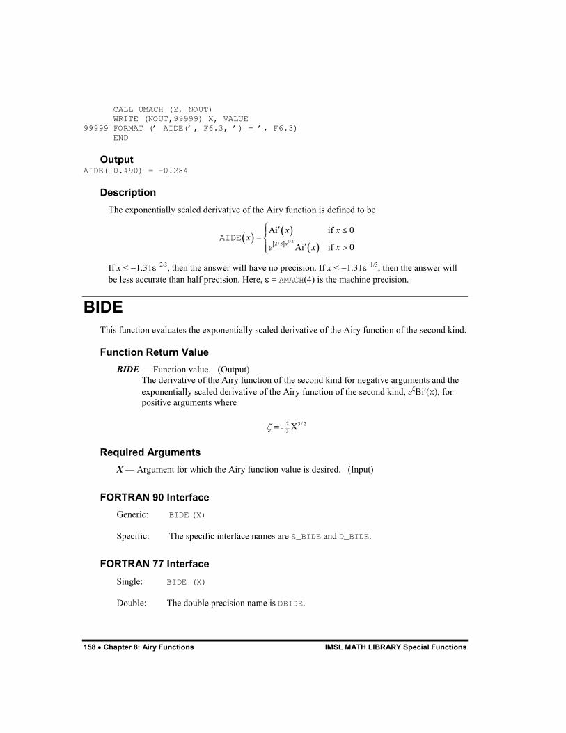
158 � Chapter 8: Airy Functions IMSL MATH LIBRARY Special Functions
CALL UMACH (2, NOUT) WRITE (NOUT,99999) X, VALUE 99999 FORMAT (� AIDE(�, F6.3, �) = �, F6.3) END
Output AIDE( 0.490) = -0.284
Description The exponentially scaled derivative of the Airy function is defined to be
� �� �
� � � �3/ 22 / 3
Ai if 0
Ai if 0x
x xx
e x x
� � ��� �
� ���
AIDE
If x < �1.31�����, then the answer will have no precision. If x < �1.31�����, then the answer will be less accurate than half precision. Here, � = AMACH(4) is the machine precision.
BIDE This function evaluates the exponentially scaled derivative of the Airy function of the second kind.
Function Return Value BIDE � Function value. (Output)
The derivative of the Airy function of the second kind for negative arguments and the exponentially scaled derivative of the Airy function of the second kind, e�Bi�(X), for positive arguments where
2 3 / 23 X� ��
Required Arguments X � Argument for which the Airy function value is desired. (Input)
FORTRAN 90 Interface Generic: BIDE (X)
Specific: The specific interface names are S_BIDE and D_BIDE.
FORTRAN 77 Interface Single: BIDE (X)
Double: The double precision name is DBIDE.
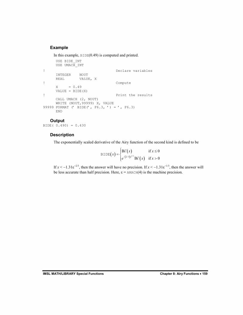
IMSL MATH/LIBRARY Special Functions Chapter 8: Airy Functions � 159
Example In this example, BIDE(0.49) is computed and printed.
USE BIDE_INT USE UMACH_INT
! Declare variables INTEGER NOUT REAL VALUE, X ! Compute X = 0.49 VALUE = BIDE(X) ! Print the results CALL UMACH (2, NOUT) WRITE (NOUT,99999) X, VALUE 99999 FORMAT (� BIDE(�, F6.3, �) = �, F6.3) END
Output BIDE( 0.490) = 0.430
Description The exponentially scaled derivative of the Airy function of the second kind is defined to be
� �� �
� � � �3/ 22 / 3
Bi if 0
Bi if 0x
x xx
e x x�
� � ��� �
� ���
BIDE
If x < �1.31�����, then the answer will have no precision. If x < �1.31�����, then the answer will be less accurate than half precision. Here, � = AMACH(4) is the machine precision.

160 � Chapter 8: Airy Functions IMSL MATH LIBRARY Special Functions
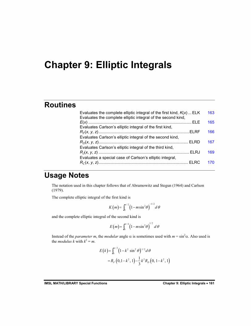
IMSL MATH/LIBRARY Special Functions Chapter 9: Elliptic Integrals � 161
Chapter 9: Elliptic Integrals
Routines Evaluates the complete elliptic integral of the first kind, K(x) ... ELK 163 Evaluates the complete elliptic integral of the second kind, E(x) ........................................................................................... ELE 165 Evaluates Carlson�s elliptic integral of the first kind, RF(x, y, z) ................................................................................ELRF 166 Evaluates Carlson�s elliptic integral of the second kind, RD(x, y, z)............................................................................... ELRD 167 Evaluates Carlson�s elliptic integral of the third kind, RJ(x, y, z) ................................................................................ ELRJ 169 Evaluates a special case of Carlson�s elliptic integral, RC(x, y, z)............................................................................... ELRC 170
Usage Notes The notation used in this chapter follows that of Abramowitz and Stegun (1964) and Carlson (1979).
The complete elliptic integral of the first kind is
� � � �1/ 2/ 2 2
01 sinK m m d
�
� ��
� ��
and the complete elliptic integral of the second kind is
� � � �1/ 2/ 2 2
01 sinE m m d
�
� �� ��
Instead of the parameter m, the modular angle is sometimes used with m = sin�. Also used is the modulus k with k� = m.
� � � �
� � � �
/ 2 2 2 1/ 2
0
2 2 2
1 sin
10,1 , 1 0, 1 , 13F D
E k k d
R k k R k
�
� �� �
� � � �
�
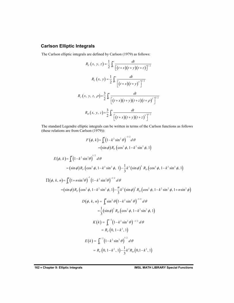
162 � Chapter 9: Elliptic Integrals IMSL MATH LIBRARY Special Functions
Carlson Elliptic Integrals The Carlson elliptic integrals are defined by Carlson (1979) as follows:
� �� �� �� �
1/ 20
1, ,2F
dtR x y zt x t y t z
�
�� � �� �� �
�
� �� �� �
1/ 20 2
1,2C
dtR x yt x t y
�
�� �� �� �
�
� �� �� �� �� �
1/ 20 2
3, , ,2J
dtR x y zt x t y t z t
�
�
�
�� �� � � �� �
�
� �� �� �� �
1/ 20 3
3, ,2D
dtR x y zt x t y t z
�
�� �� � �� �
�
The standard Legendre elliptic integrals can be written in terms of the Carlson functions as follows (these relations are from Carlson (1979)):
� � � �
� � � �
1/ 22 2
0
2 2 2
, 1 sin
sin cos , 1 sin , 1F
F k k d
R k
�
� � �
� � �
�
� �
� �
�
� � � �
� � � � � � � �
1/ 22 2
0
32 2 2 2 2 2 2
, 1 sin
1sin cos , 1 sin , 1 sin cos , 1 sin , 13F D
E k k d
R k k R k
�
� � �
� � � � � �
� �
� � � �
�
� � � � � �
� � � � � � � �
1 1/ 22 2 2
0
32 2 2 2 2 2 2 2
, , 1 sin 1 sin
sin cos , 1 sin , 1 sin cos , 1 sin , 1 sin3F D
k n n k d
nR k k R k n
�
� � � �
� � � � � � �
�
�
� � � �
� � � � �
�
� � � �
� � � �
1/ 22 2 2
0
3 2 2 2
, , sin 1 sin
1 sin cos , 1 sin , 13 D
D k n k d
R k
�
� � � �
� � �
�
� �
� �
�
� � � �
� �
/ 2 2 2 1/ 2
0
2
1 sin
0, 1 , 1F
K k k d
R k
�
� ��
� �
� �
�
� � � �
� � � �
1/ 2/ 2 2 2
0
2 2 2
1 sin
10, 1 , 1 0,1 , 13F D
E k k d
R k k R k
�
� �� �
� � � �
�
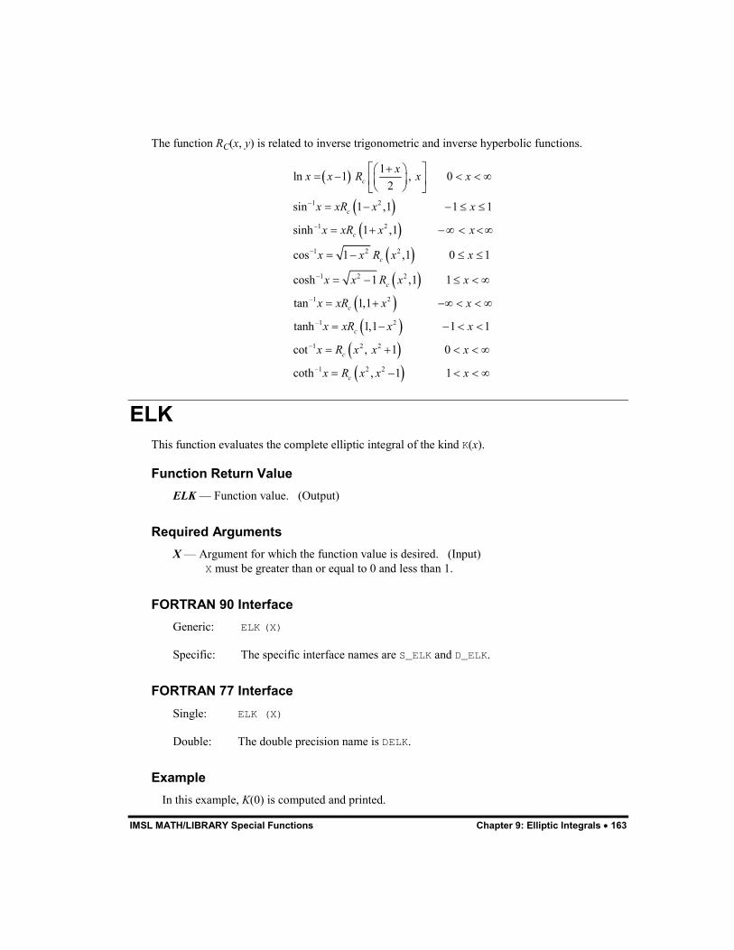
IMSL MATH/LIBRARY Special Functions Chapter 9: Elliptic Integrals � 163
The function RC(x, y) is related to inverse trigonometric and inverse hyperbolic functions.
� �
� �
� �
� �
� �
� �
� �
� �
1 2
1 2
1 2 2
1 2 2
1 2
1 2
1 2 2
1
1ln 1 , 02
sin 1 ,1 1 1
sinh 1 ,1
cos 1 ,1 0 1
cosh 1 ,1 1
tan 1,1
tanh 1,1 1 1
cot , 1 0
coth
c
c
c
c
c
c
c
c
c
xx x R x x
x xR x x
x xR x x
x x R x x
x x R x x
x xR x x
x xR x x
x R x x x
x R x
�
�
�
�
�
�
�
�
� � �� �� � � � ��
� �� �
� � � � �
� � � � �
� � � �
� � � �
� � � � �
� � � � �
� � � �
� � �2 2, 1 1x x� � �
ELK This function evaluates the complete elliptic integral of the kind K(x).
Function Return Value ELK � Function value. (Output)
Required Arguments X � Argument for which the function value is desired. (Input)
X must be greater than or equal to 0 and less than 1.
FORTRAN 90 Interface Generic: ELK (X)
Specific: The specific interface names are S_ELK and D_ELK.
FORTRAN 77 Interface Single: ELK (X)
Double: The double precision name is DELK.
Example In this example, K(0) is computed and printed.

164 � Chapter 9: Elliptic Integrals IMSL MATH LIBRARY Special Functions
USE ELK_INT USE UMACH_INT ! Declare variables INTEGER NOUT REAL VALUE, X ! Compute X = 0.0 VALUE = ELK(X) ! Print the results CALL UMACH (2, NOUT) WRITE (NOUT,99999) X, VALUE 99999 FORMAT (� ELK(�, F6.3, �) = �, F6.3) END
Output ELK( 0.000) = 1.571
Description The complete elliptic integral of the first kind is defined to be
� �/ 2
1/ 20 2for 0 1
1 sin
dK x xx
� �
�
� � �� ��� �
�
The argument x must satisfy 0 � x < 1; otherwise, ELK is set to b = AMACH(2), the largest representable floating-point number.
The function K(x) is computed using the routine ELRF (page 166) and the relation K(x) = RF(0, 1 � x, 1).
Figure 9-1 Plot of K(x) and E(x)
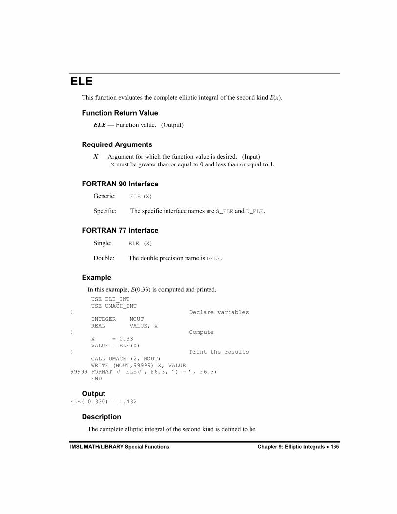
IMSL MATH/LIBRARY Special Functions Chapter 9: Elliptic Integrals � 165
ELE This function evaluates the complete elliptic integral of the second kind E(x).
Function Return Value ELE � Function value. (Output)
Required Arguments X � Argument for which the function value is desired. (Input)
X must be greater than or equal to 0 and less than or equal to 1.
FORTRAN 90 Interface Generic: ELE (X)
Specific: The specific interface names are S_ELE and D_ELE.
FORTRAN 77 Interface Single: ELE (X)
Double: The double precision name is DELE.
Example In this example, E(0.33) is computed and printed.
USE ELE_INT USE UMACH_INT ! Declare variables INTEGER NOUT REAL VALUE, X ! Compute X = 0.33 VALUE = ELE(X) ! Print the results CALL UMACH (2, NOUT) WRITE (NOUT,99999) X, VALUE 99999 FORMAT (� ELE(�, F6.3, �) = �, F6.3) END
Output ELE( 0.330) = 1.432
Description The complete elliptic integral of the second kind is defined to be
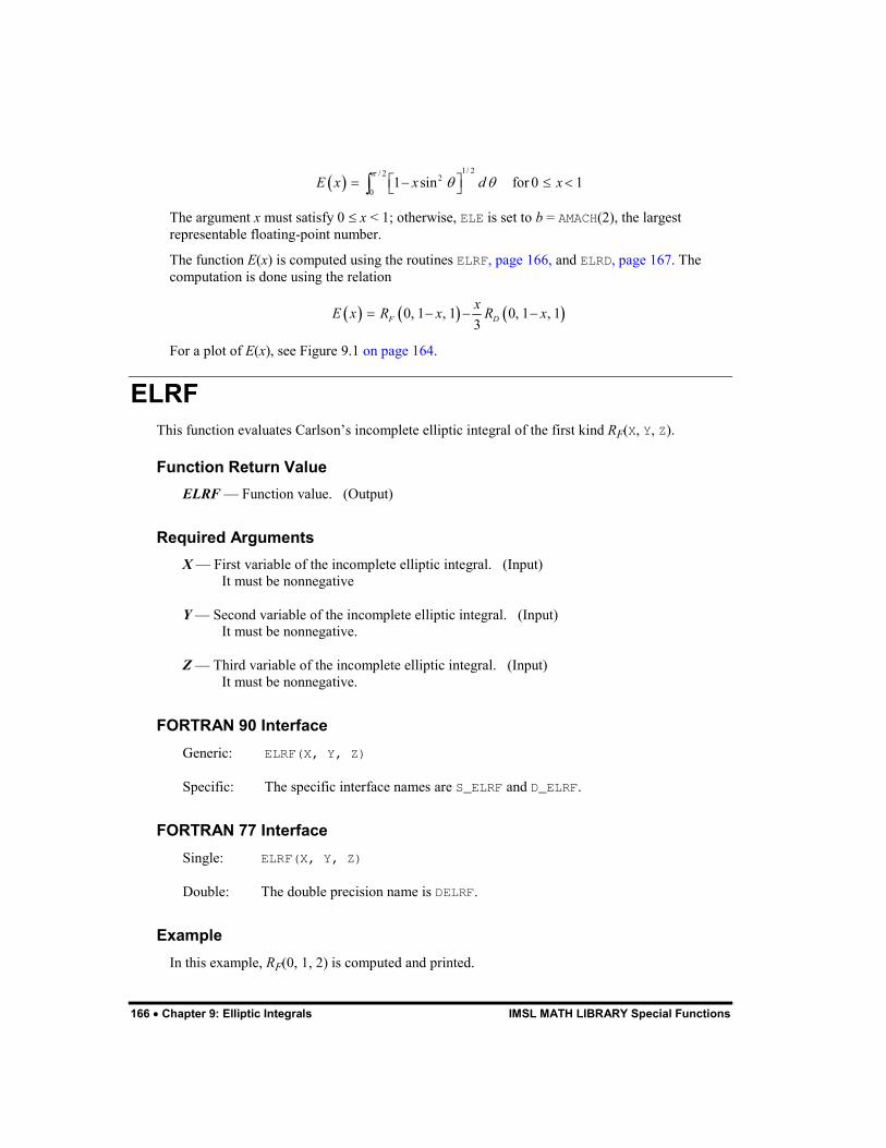
166 � Chapter 9: Elliptic Integrals IMSL MATH LIBRARY Special Functions
� �1/ 2/ 2 2
01 sin for 0 1E x x d x
�
� �� �� � � �� ��
The argument x must satisfy 0 � x < 1; otherwise, ELE is set to b = AMACH(2), the largest representable floating-point number.
The function E(x) is computed using the routines ELRF, page 166, and ELRD, page 167. The computation is done using the relation
� � � � � �0, 1 , 1 0, 1 , 13F DxE x R x R x� � � �
For a plot of E(x), see Figure 9.1 on page 164.
ELRF This function evaluates Carlson�s incomplete elliptic integral of the first kind RF(X, Y, Z).
Function Return Value ELRF � Function value. (Output)
Required Arguments X � First variable of the incomplete elliptic integral. (Input)
It must be nonnegative
Y � Second variable of the incomplete elliptic integral. (Input) It must be nonnegative.
Z � Third variable of the incomplete elliptic integral. (Input) It must be nonnegative.
FORTRAN 90 Interface Generic: ELRF(X, Y, Z)
Specific: The specific interface names are S_ELRF and D_ELRF.
FORTRAN 77 Interface Single: ELRF(X, Y, Z)
Double: The double precision name is DELRF.
Example In this example, RF(0, 1, 2) is computed and printed.
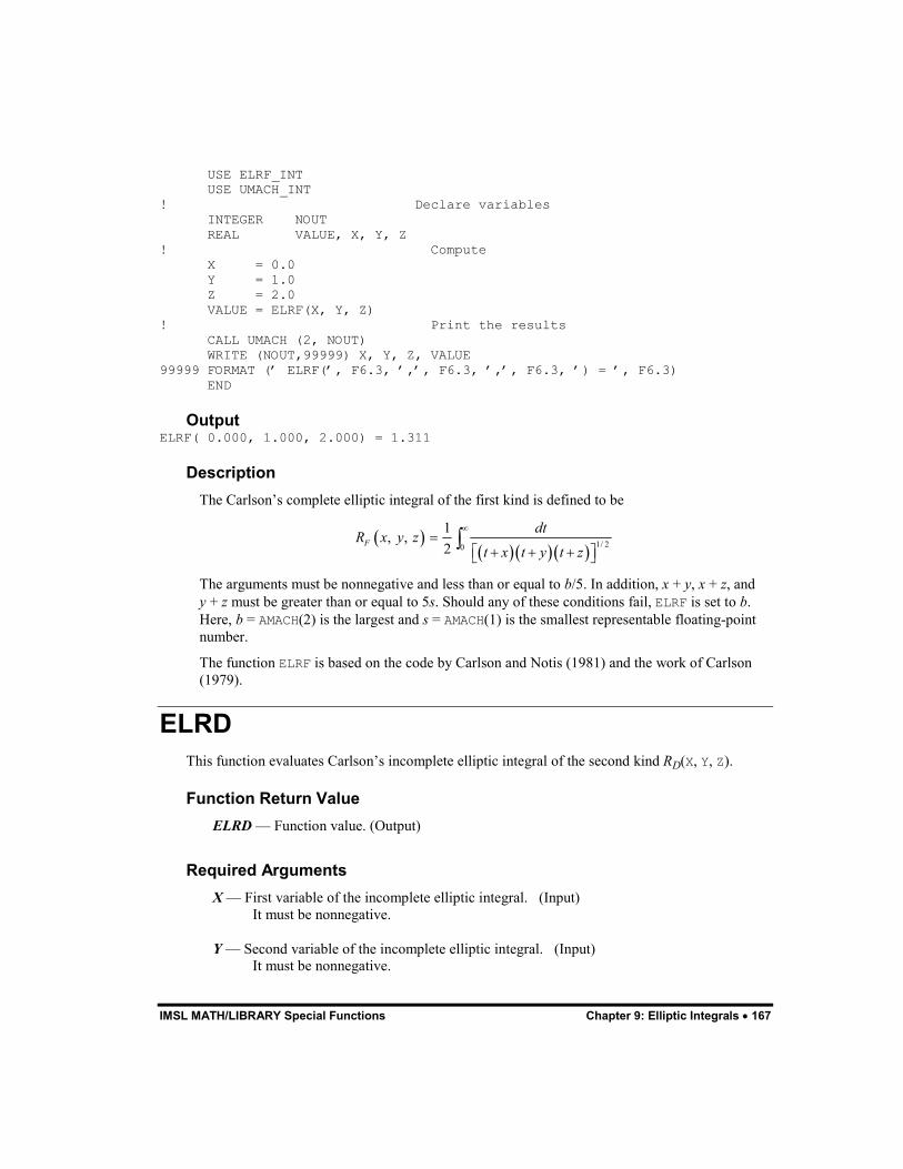
IMSL MATH/LIBRARY Special Functions Chapter 9: Elliptic Integrals � 167
USE ELRF_INT USE UMACH_INT ! Declare variables INTEGER NOUT REAL VALUE, X, Y, Z ! Compute X = 0.0 Y = 1.0 Z = 2.0 VALUE = ELRF(X, Y, Z) ! Print the results CALL UMACH (2, NOUT) WRITE (NOUT,99999) X, Y, Z, VALUE 99999 FORMAT (� ELRF(�, F6.3, �,�, F6.3, �,�, F6.3, �) = �, F6.3) END
Output ELRF( 0.000, 1.000, 2.000) = 1.311
Description The Carlson�s complete elliptic integral of the first kind is defined to be
� �� �� �� �
1/ 20
1, ,2F
dtR x y zt x t y t z
�
�� � �� �� �
�
The arguments must be nonnegative and less than or equal to b/5. In addition, x + y, x + z, and y + z must be greater than or equal to 5s. Should any of these conditions fail, ELRF is set to b. Here, b = AMACH(2) is the largest and s = AMACH(1) is the smallest representable floating-point number.
The function ELRF is based on the code by Carlson and Notis (1981) and the work of Carlson (1979).
ELRD This function evaluates Carlson�s incomplete elliptic integral of the second kind RD(X, Y, Z).
Function Return Value ELRD � Function value. (Output)
Required Arguments X � First variable of the incomplete elliptic integral. (Input)
It must be nonnegative.
Y � Second variable of the incomplete elliptic integral. (Input) It must be nonnegative.

168 � Chapter 9: Elliptic Integrals IMSL MATH LIBRARY Special Functions
Z � Third variable of the incomplete elliptic integral. (Input) It must be positive.
FORTRAN 90 Interface Generic: ELRD(X, Y, Z)
Specific: The specific interface names are S_ELRD and D_ELRD.
FORTRAN 77 Interface Single: ELRD(X, Y, Z)
Double: The double precision name is DELRD.
Example In this example, RD(0, 2, 1) is computed and printed.
USE ELRD_INT USE UMACH_INT ! Declare variables INTEGER NOUT REAL VALUE, X, Y, Z ! Compute X = 0.0 Y = 2.0 Z = 1.0 VALUE = ELRD(X, Y, Z) ! Print the results CALL UMACH (2, NOUT) WRITE (NOUT,99999) X, Y, Z, VALUE 99999 FORMAT (� ELRD(�, F6.3, �,�, F6.3, �,�, F6.3, �) = �, F6.3) END
Output ELRD( 0.000, 2.000, 1.000) = 1.797
Description The Carlson�s complete elliptic integral of the second kind is defined to be
� �� �� � � �
1/ 20 3
3, ,2D
dtR x y zt x t y t z
�
�� �� � �� �
�
The arguments must be nonnegative and less than or equal to 0.69(�ln �)��� s���� where � = AMACH(4) is the machine precision, s = AMACH(1) is the smallest representable positive number. Furthermore, x + y and z must be greater than max{3s���, 3/b���}, where b = AMACH(2) is the largest floating-point number. If any of these conditions are false, then ELRD is set to b.

IMSL MATH/LIBRARY Special Functions Chapter 9: Elliptic Integrals � 169
The function ELRD is based on the code by Carlson and Notis (1981) and the work of Carlson (1979).
ELRJ This function evaluates Carlson�s incomplete elliptic integral of the third kind RJ(X, Y, Z, RHO)
Function Return Value ELRJ � Function value. (Output)
Required Arguments X � First variable of the incomplete elliptic integral. (Input)
It must be nonnegative.
Y � Second variable of the incomplete elliptic integral. (Input) It must be nonnegative.
Z � Third variable of the incomplete elliptic integral. (Input) It must be nonnegative.
RHO � Fourth variable of the incomplete elliptic integral. (Input) It must be positive.
FORTRAN 90 Interface Generic: ELRJ(X, Y, Z, RHO)
Specific: The specific interface names are S_ELRJ and D_ELRJ.
FORTRAN 77 Interface Single: ELRJ(X, Y, Z, RHO)
Double: The double precision name is DELRJ.
Example In this example, RJ(2, 3, 4, 5) is computed and printed.
USE ELRJ_INT USE UMACH_INT ! Declare variables INTEGER NOUT REAL RHO, VALUE, X, Y, Z ! Compute X = 2.0
170 � Chapter 9: Elliptic Integrals IMSL MATH LIBRARY Special Functions
Y = 3.0 Z = 4.0 RHO = 5.0 VALUE = ELRJ(X, Y, Z, RHO) ! Print the results CALL UMACH (2, NOUT) WRITE (NOUT,99999) X, Y, Z, RHO, VALUE 99999 FORMAT (� ELRJ(�, F6.3, �,�, F6.3, �,�, F6.3, �,�, F6.3, & �) = �, F6.3) END
Output ELRJ( 2.000, 3.000, 4.000, 5.000) = 0.143
Description The Carlson�s complete elliptic integral of the third kind is defined to be
� �� � � �� �� �
1/ 20 2
3, , ,2J
dtR x y zt x t y t z t
�
�
�
�� �� � � �� �
�
The arguments must be nonnegative. In addition, x + y, x + z, y + z and � must be greater than or equal to (5s)��� and less than or equal to .3(b/5)���, where s = AMACH(1) is the smallest representable floating-point number. Should any of these conditions fail, ELRF is set to b = AMACH(2), the largest floating-point number.
The function ELRJ is based on the code by Carlson and Notis (1981) and the work of Carlson (1979).
ELRC This function evaluates an elementary integral from which inverse circular functions, logarithms and inverse hyperbolic functions can be computed.
Function Return Value ELRC � Function value. (Output)
Required Arguments X � First variable of the incomplete elliptic integral. (Input)
It must be nonnegative and satisfy the conditions given in Comments.
Y � Second variable of the incomplete elliptic integral. (Input) It must be positive and satisfy the conditions given in Comments.
FORTRAN 90 Interface Generic: ELRC(X, Y)
IMSL MATH/LIBRARY Special Functions Chapter 9: Elliptic Integrals � 171
Specific: The specific interface names are S_ELRC and D_ELRC.
FORTRAN 77 Interface Single: ELRC(X, Y)
Double: The double precision name is DELRC.
Example In this example, RC(2.25, 2.0) is computed and printed.
USE ELRC_INT USE UMACH_INT ! Declare variables INTEGER NOUT REAL VALUE, X, Y ! Compute X = 0.0 Y = 1.0 VALUE = ELRC(X, Y) ! Print the results CALL UMACH (2, NOUT) WRITE (NOUT,99999) X, Y, VALUE 99999 FORMAT (� ELRC(�, F6.3, �,�, F6.3, �) = �, F6.3) END
Output ELRC( 0.000, 1.000) = 1.571
Comments The sum X + Y must be greater than or equal to ARGMIN and both X and Y must be less than or equal to ARGMAX. ARGMIN = s * 5 and ARGMAX = b/5, where s is the machine minimum (AMACH(1)) and b is the machine maximum (AMACH(2)).
Description The special case of Carlson�s complete elliptic integral of the first kind is defined to be
� �� �� �
1/ 20 2
1,2C
dtR x yt x t y
�
�� �� �� �
�
The argument x must be nonnegative, y must be positive, and x + y must be less than or equal to b/5 and greater than or equal to 5s. If any of these conditions are false, then ELRC is set to b. Here, b = AMACH(2) is the largest and s = AMACH(1) is the smallest representable floating-point number.
The function ELRC is based on the code by Carlson and Notis (1981) and the work of Carlson (1979).

172 � Chapter 9: Elliptic Integrals IMSL MATH LIBRARY Special Functions
IMSL MATH/LIBRARY Special Functions Chapter 10: Elliptic and Related Functions � 173
Chapter 10: Elliptic and Related Functions
Routines 10.1. Weierstrass Elliptic and Related Functions
Lemninscatic case .................................................................CWPL 173 Lemninscatic case derivative..............................................CWPLD 175 Equianharmonic case ...........................................................CWPQ 176 Equianharmonic case derivative........................................ CWPQD 177
10.2. Jacobi Elliptic Functions Jacobi function sn(x, m) (real argument) ................................EJSN 178 Jacobi function cn(x, m) (real argument) ................................EJCN 180 Jacobi function dn(x, m) (real argument)................................EJDN 182
Usage Notes Elliptic functions are doubly periodic, single-valued complex functions of a single variable that are analytic, except at a finite number of poles. Because of the periodicity, we need consider only the fundamental period parallelogram. The irreducible number of poles, counting multiplicities, is the order of the elliptic function. The simplest, non-trivial, elliptic functions are of order two.
The Weierstrass elliptic functions, �(z, �, ��) have a double pole at z = 0 and so are of order two. Here, 2� and 2�� are the periods.
The Jacobi elliptic functions each have two simple poles and so are also of order two. The period of the functions is as follows:
Function Periods sn(x, m) 4K(m) 2iK�(m) cn(x, m) 4K(m) 4iK�(m) dn(x, m) 2K(m) 4iK�(m)
The function K(m) is the complete elliptic integral, see ELK (page 163), and K�(m) = K(1 � m).
CWPL This function evaluates the Weierstrass� � function in the lemniscatic case for complex argument with unit period parallelogram.
174 � Chapter 10: Elliptic and Related Functions IMSL MATH/LIBRARY Special Functions
Function Return Value CWPL � Complex function value. (Output)
Required Arguments Z � Complex argument for which the function value is desired. (Input)
FORTRAN 90 Interface Generic: CWPL (Z)
Specific: The specific interface names are C_CWPL and Z_CWPL.
FORTRAN 77 Interface Complex: CWPL (Z)
Double complex: The double complex name is ZWPL.
Example In this example, �(0.25 + 0.25i) is computed and printed.
USE CWPL_INT USE UMACH_INT ! Declare variables INTEGER NOUT COMPLEX VALUE, Z ! Compute Z = (0.25, 0.25) VALUE = CWPL(Z) ! Print the results CALL UMACH (2, NOUT) WRITE (NOUT,99999) Z, VALUE 99999 FORMAT (� CWPL(�, F6.3, �,�, F6.3, �) = (�, & F6.3, �,�, F6.3, �)�) END
Output CWPL( 0.250, 0.250) = ( 0.000,-6.875)
Description The Weierstrass� � function, �(z) = �(z | �, ��), is an elliptic function of order two with periods 2� and 2�� and a double pole at z = 0. CWPL(Z) computes �(z | �, ��) with 2� = 1 and 2�� = i.
The input argument is first reduced to the fundamental parallelogram of all z satisfying �1/2 � �z � 1/2 and �1/2 � z � 1/2. Then, a rational approximation is used.
All arguments are valid with the exception of the lattice points z = m + ni, which are the poles of CWPL. If the argument is a lattice point, then b = AMACH(2) , the largest floating-point number, is
IMSL MATH/LIBRARY Special Functions Chapter 10: Elliptic and Related Functions � 175
returned. If the argument has modulus greater than 10���, then NaN (not a number) is returned. Here, � = AMACH(4) is the machine precision.
Function CWPL is based on code by Eckhardt (1980). Also, see Eckhardt (1977).
CWPLD This function evaluates the first derivative of the Weierstrass� � function in the lemniscatic case for complex argument with unit period parallelogram.
Function Return Value CWPLD � Complex function value. (Output)
Required Arguments Z � Complex argument for which the function value is desired. (Input)
FORTRAN 90 Interface Generic: CWPLD (Z)
Specific: The specific interface names are C_CWPLD and Z_CWPLD.
FORTRAN 77 Interface Complex: CWPLD (Z)
Double complex: The double complex name is ZWPLD.
Example In this example, �(0.25 + 0.25i) is computed and printed.
USE CWPLD_INT USE UMACH_INT ! Declare variables INTEGER NOUT COMPLEX VALUE, Z ! Compute Z = (0.25, 0.25) VALUE = CWPLD(Z) ! Print the results CALL UMACH (2, NOUT) WRITE (NOUT,99999) Z, VALUE 99999 FORMAT (� CWPLD(�, F6.3, �,�, F6.3, �) = (�, & F6.3, �,�, F6.3, �)�) END
Output CWPLD( 0.250, 0.250) = (36.054,36.054)
176 � Chapter 10: Elliptic and Related Functions IMSL MATH/LIBRARY Special Functions
Description The Weierstrass� � function, �(z) = �(z | �, ��), is an elliptic function of order two with periods 2� and 2�� and a double pole at z = 0. CWPLD(Z) computes the derivative of �(z | �, ��) with 2� = 1 and 2�� = i. CWPL, page 173, computes �(z | �, ��).
The input argument is first reduced to the fundamental parallelogram of all z satisfying �1/2 � �z � 1/2 and �1/2 � z � 1/2. Then, a rational approximation is used.
All arguments are valid with the exception of the lattice points z = m + ni, which are the poles of CWPL. If the argument is a lattice point, then b = AMACH(2), the largest floating-point number, is returned.
Function CWPLD is based on code by Eckhardt (1980). Also, see Eckhardt (1977).
CWPQ This function evaluates the Weierstrass� � function in the equianharmonic case for complex argument with unit period parallelogram.
Function Return Value CWPQ � Complex function value. (Output)
Required Arguments Z � Complex argument for which the function value is desired. (Input)
FORTRAN 90 Interface Generic: CWPQ (Z)
Specific: The specific interface names are C_CWPQ and Z_CWPQ.
FORTRAN 77 Interface Complex: CWPQ (Z)
Double complex: The double complex name is ZWPQ.
Example In this example, �(0.25 + 0.14437567i) is computed and printed.
USE CWPQ_INT USE UMACH_INT ! Declare variables INTEGER NOUT COMPLEX VALUE, Z ! Compute Z = (0.25, 0.14437567) VALUE = CWPQ(Z) ! Print the results
IMSL MATH/LIBRARY Special Functions Chapter 10: Elliptic and Related Functions � 177
CALL UMACH (2, NOUT) WRITE (NOUT,99999) Z, VALUE 99999 FORMAT (� CWPQ(�, F6.3, �,�, F6.3, �) = (�, & F7.3, �,�, F7.3, �)�) END
Output CWPQ( 0.250, 0.144) = ( 5.895,-10.216)
Description The Weierstrass� � function, �(z) = �(z | �, ��), is an elliptic function of order two with periods 2� and 2�� and a double pole at z = 0. CWPQ(Z) computes �(z | �, ��) with
4 1 3 and 4 1 3i i� � �� � � �
The input argument is first reduced to the fundamental parallelogram of all z satisfying
1/ 2 1/ 2 and 3 / 4 3 / 4z z� � � � � � � �
Then, a rational approximation is used.
All arguments are valid with the exception of the lattice points
� � � �1 3 1 3z m i n i� � � �
which are the poles of CWPQ. If the argument is a lattice point, then b = AMACH(2), the largest floating-point number, is returned. If the argument has modulus greater than 10���, then NaN (not a number) is returned. Here, � = AMACH(4) is the machine precision.
Function CWPQ is based on code by Eckhardt (1980). Also, see Eckhardt (1977).
CWPQD This function evaluates the first derivative of the Weierstrass� � function in the equianharmonic case for complex argument with unit period parallelogram.
Function Return Value CWPQD � Complex function value. (Output)
Required Arguments Z � Complex argument for which the function value is desired. (Input)
FORTRAN 90 Interface Generic: CWPQD (Z)
Specific: The specific interface names are C_CWPQD and Z_CWPQD.
178 � Chapter 10: Elliptic and Related Functions IMSL MATH/LIBRARY Special Functions
FORTRAN 77 Interface Complex: CWPQD (Z)
Double complex: The double complex name is ZWPQD.
Example In this example, �(0.25 + 0.14437567i) is computed and printed.
USE CWPQD_INT USE UMACH_INT ! Declare variables INTEGER NOUT COMPLEX VALUE, Z ! Compute Z = (0.25, 0.14437567) VALUE = CWPQD(Z) ! Print the results CALL UMACH (2, NOUT) WRITE (NOUT,99999) Z, VALUE 99999 FORMAT (� CWPQD(�, F6.3, �,�, F6.3, �) = (�, & F6.3, �,�, F6.3, �)�) END
Output CWPQD( 0.250, 0.144) = ( 0.028,85.934)
Description The Weierstrass� � function, �(z) = �(z | �, ��), is an elliptic function of order two with periods 2� and 2�� and a double pole at z = 0. CWPQD(Z) computes the derivative of �(z | �, ��) with
4 1 3 and 4 1 3i i� � �� � � �
CWPQ, page 176, computes �(z | �, ��).
The input argument is first reduced to the fundamental parallelogram of all z satisfying
1/ 2 1/ 2 and 3 / 4 3 / 4z z� � � � � � � �
Then, a rational approximation is used.
All arguments are valid with the exception of the lattice points
� � � �1 3 1 3z m i n i� � � �
which are the poles of CWPQ. If the argument is a lattice point, then b = AMACH(2), the largest floating-point number, is returned.
Function CWPQD is based on code by Eckhardt (1980). Also, see Eckhardt (1977).
EJSN This function evaluates the Jacobi elliptic function sn(x, m).
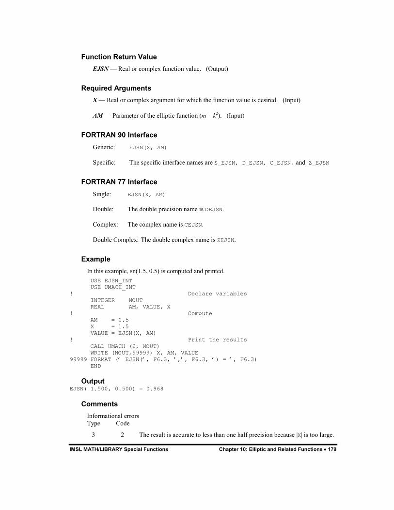
IMSL MATH/LIBRARY Special Functions Chapter 10: Elliptic and Related Functions � 179
Function Return Value EJSN � Real or complex function value. (Output)
Required Arguments X � Real or complex argument for which the function value is desired. (Input)
AM � Parameter of the elliptic function (m = k�). (Input)
FORTRAN 90 Interface Generic: EJSN(X, AM)
Specific: The specific interface names are S_EJSN, D_EJSN, C_EJSN, and Z_EJSN
FORTRAN 77 Interface Single: EJSN(X, AM)
Double: The double precision name is DEJSN.
Complex: The complex name is CEJSN.
Double Complex: The double complex name is ZEJSN.
Example In this example, sn(1.5, 0.5) is computed and printed.
USE EJSN_INT USE UMACH_INT ! Declare variables INTEGER NOUT REAL AM, VALUE, X ! Compute AM = 0.5 X = 1.5 VALUE = EJSN(X, AM) ! Print the results CALL UMACH (2, NOUT) WRITE (NOUT,99999) X, AM, VALUE 99999 FORMAT (� EJSN(�, F6.3, �,�, F6.3, �) = �, F6.3) END
Output EJSN( 1.500, 0.500) = 0.968
Comments Informational errors Type Code
3 2 The result is accurate to less than one half precision because |X| is too large.
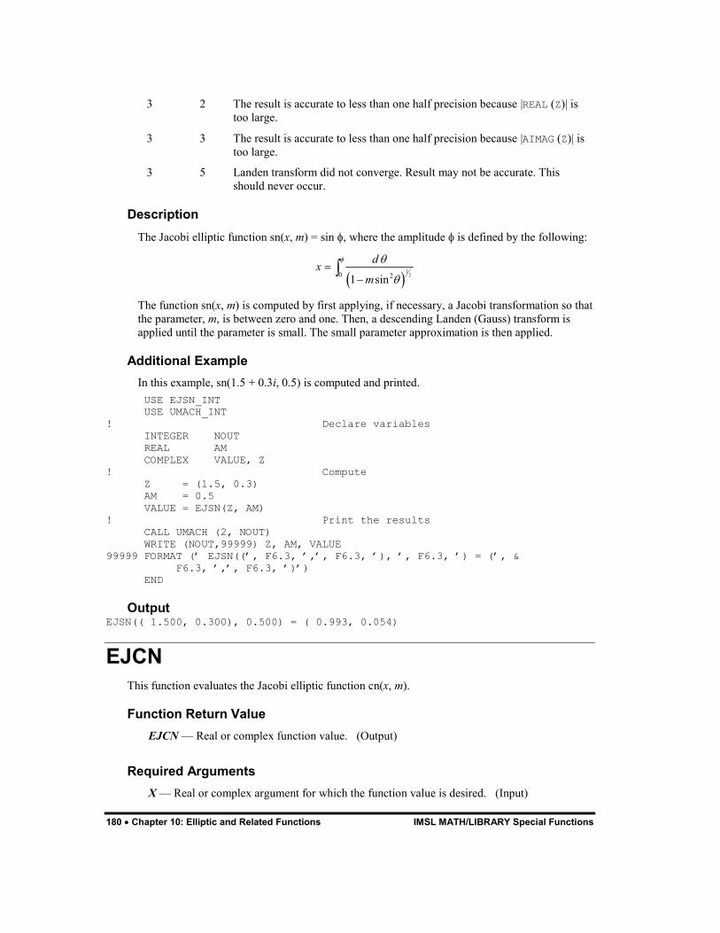
180 � Chapter 10: Elliptic and Related Functions IMSL MATH/LIBRARY Special Functions
3 2 The result is accurate to less than one half precision because |REAL (Z)| is too large.
3 3 The result is accurate to less than one half precision because |AIMAG (Z)| is too large.
3 5 Landen transform did not converge. Result may not be accurate. This should never occur.
Description The Jacobi elliptic function sn(x, m) = sin , where the amplitude is defined by the following:
� �1
20 21 sin
dxm
� �
�
�
�
�
The function sn(x, m) is computed by first applying, if necessary, a Jacobi transformation so that the parameter, m, is between zero and one. Then, a descending Landen (Gauss) transform is applied until the parameter is small. The small parameter approximation is then applied.
Additional Example In this example, sn(1.5 + 0.3i, 0.5) is computed and printed.
USE EJSN_INT USE UMACH_INT ! Declare variables INTEGER NOUT REAL AM COMPLEX VALUE, Z ! Compute Z = (1.5, 0.3) AM = 0.5 VALUE = EJSN(Z, AM) ! Print the results CALL UMACH (2, NOUT) WRITE (NOUT,99999) Z, AM, VALUE 99999 FORMAT (� EJSN((�, F6.3, �,�, F6.3, �), �, F6.3, �) = (�, & F6.3, �,�, F6.3, �)�) END
Output EJSN(( 1.500, 0.300), 0.500) = ( 0.993, 0.054)
EJCN This function evaluates the Jacobi elliptic function cn(x, m).
Function Return Value EJCN � Real or complex function value. (Output)
Required Arguments X � Real or complex argument for which the function value is desired. (Input)

IMSL MATH/LIBRARY Special Functions Chapter 10: Elliptic and Related Functions � 181
AM � Parameter of the elliptic function (m = k2). (Input)
FORTRAN 90 Interface Generic: EJCN(X, AM)
Specific: The specific interface names are S_EJCN, D_EJCN, C_EJCN, and Z_EJCN.
FORTRAN 77 Interface Single: EJCN(X, AM)
Double: The double precision name is DEJCN.
Complex: The complex name is CEJCN.
Double Complex: The double complex name is ZEJCN.
Example In this example, cn(1.5, 0.5) is computed and printed.
USE EJCN_INT USE UMACH_INT ! Declare variables INTEGER NOUT REAL AM, VALUE, X ! Compute AM = 0.5 X = 1.5 VALUE = EJCN(X, AM) ! Print the results CALL UMACH (2, NOUT) WRITE (NOUT,99999) X, AM, VALUE 99999 FORMAT (� EJCN(�, F6.3, �,�, F6.3, �) = �, F6.3) END
Output EJCN( 1.500, 0.500) = 0.250
Comments Informational errors Type Code
3 2 The result is accurate to less than one half precision because |X| is too large.
3 2 The result is accurate to less than one half precision because |REAL (Z)| is too large.
3 3 The result is accurate to less than one half precision because |AIMAG (Z)| is too large.
3 5 Landen transform did not converge. Result may not be accurate. This should never occur.

182 � Chapter 10: Elliptic and Related Functions IMSL MATH/LIBRARY Special Functions
Description The Jacobi elliptic function cn(x, m) = cos , where the amplitude is defined by the following:
� �1
20 21 sin
dxm
� �
�
�
�
�
The function cn(x, m) is computed by first applying, if necessary, a Jacobi transformation so that the parameter, m, is between zero and one. Then, a descending Landen (Gauss) transform is applied until the parameter is small. The small parameter approximation is then applied.
Additional Example In this example, cn(1.5 + 0.3i, 0.5) is computed and printed.
USE EJCN_INT USE UMACH_INT ! Declare variables INTEGER NOUT REAL AM COMPLEX VALUE, Z ! Compute Z = (1.5, 0.3) AM = 0.5 VALUE = EJCN(Z, AM) ! Print the results CALL UMACH (2, NOUT) WRITE (NOUT,99999) Z, AM, VALUE 99999 FORMAT (� EJCN((�, F6.3, �,�, F6.3, �), �, F6.3, �) = (�, & F6.3, �,�, F6.3, �)�) END
Output EJCN(( 1.500, 0.300), 0.500) = ( 0.251,-0.212)
EJDN This function evaluates the Jacobi elliptic function dn(x, m).
Function Return Value EJDN � Real or complex function value. (Output)
Required Arguments X � Real or complex argument for which the function value is desired. (Input)
AM � Parameter of the elliptic function (m = k�). (Input)
FORTRAN 90 Interface Generic: EJDN(X, AM)
Specific: The specific interface names are S_EJDN, D_EJDN, C_EJDN, and Z_EJDN.
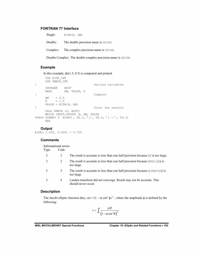
IMSL MATH/LIBRARY Special Functions Chapter 10: Elliptic and Related Functions � 183
FORTRAN 77 Interface Single: EJDN(X, AM)
Double: The double precision name is DEJDN.
Complex: The complex precision name is CEJDN.
Double Complex: The double complex precision name is ZEJDN.
Example In this example, dn(1.5, 0.5) is computed and printed.
USE EJDN_INT USE UMACH_INT ! Declare variables INTEGER NOUT REAL AM, VALUE, X ! Compute AM = 0.5 X = 1.5 VALUE = EJDN(X, AM) ! Print the results CALL UMACH (2, NOUT) WRITE (NOUT,99999) X, AM, VALUE 99999 FORMAT (� EJDN(�, F6.3, �,�, F6.3, �) = �, F6.3) END
Output EJDN( 1.500, 0.500) = 0.729
Comments Informational errors Type Code
3 2 The result is accurate to less than one half precision because |X| is too large.
3 2 The result is accurate to less than one half precision because |REAL (Z)| is too large.
3 3 The result is accurate to less than one half precision because |AIMAG (Z)| is too large.
3 5 Landen transform did not converge. Result may not be accurate. This should never occur.
Description The Jacobi elliptic function dn(x, m) = (1 � m sin2 ) 1
2 , where the amplitude is defined by the following:
� �1
20 21 sin
dxm
� �
�
�
�
�
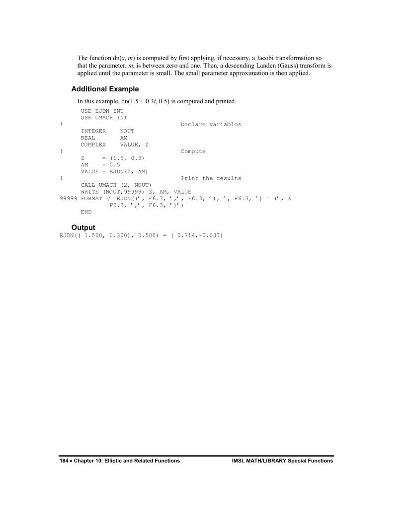
184 � Chapter 10: Elliptic and Related Functions IMSL MATH/LIBRARY Special Functions
The function dn(x, m) is computed by first applying, if necessary, a Jacobi transformation so that the parameter, m, is between zero and one. Then, a descending Landen (Gauss) transform is applied until the parameter is small. The small parameter approximation is then applied.
Additional Example In this example, dn(1.5 + 0.3i, 0.5) is computed and printed.
USE EJDN_INT USE UMACH_INT ! Declare variables INTEGER NOUT REAL AM COMPLEX VALUE, Z ! Compute Z = (1.5, 0.3) AM = 0.5 VALUE = EJDN(Z, AM) ! Print the results CALL UMACH (2, NOUT) WRITE (NOUT,99999) Z, AM, VALUE 99999 FORMAT (� EJDN((�, F6.3, �,�, F6.3, �), �, F6.3, �) = (�, & F6.3, �,�, F6.3, �)�) END
Output EJDN(( 1.500, 0.300), 0.500) = ( 0.714,-0.037)
IMSL MATH/LIBRARY Special Functions Chapter 11: Probability Distribution Functions and Inverses � 185
Chapter 11: Probability Distribution Functions and Inverses
Routines 11.1. Discrete Random Variables: Distribution Functions and Probability
Functions Binomial distribution function ................................................ BINDF 190 Binomial probability...............................................................BINPR 191 Hypergeometric distribution function ...................................HYPDF 194 Hypergeometric probability ..................................................HYPPR 196 Poisson distribution function .................................................POIDF 197 Poisson probability................................................................POIPR 199
11.2. Continuous Random Variables: Distribution Functions and Their Inverses Kolmogorov-Smirnov one-sided statistic distribution function............................................................AKS1DF 201 Kolmogorov-Smirnov two-sided statistic distribution function............................................................AKS2DF 204 Normal (Gaussian) distribution function ...........................ANORDF 206 Inverse of the normal distribution function.........................ANORIN 208 Beta distribution function ..................................................... BETDF 209 Inverse of the beta distribution function................................ BETIN 212 Bivariate normal distribution function...................................BNRDF 213 Chi-squared distribution function ..........................................CHIDF 215 Inverse of the chi-squared distribution function ..................... CHIIN 217 Noncentral chi-squared distribution function .......................CSNDF 219 F distribution function................................................................FDF 222 Inverse of the F distribution function.......................................... FIN 223 Gamma distribution function ...............................................GAMDF 225 Student’s t distribution function.................................................TDF 227 Inverse of the Student’s t distribution function........................... TIN 229 Noncentral Student’s t distribution function ........................... TNDF 231
11.3. General Continuous Random Variables Distribution function given ordinates of density .....................GCDF 233 Inverse of distribution function given ordinates of density......GCIN 236
186 � Chapter 11: Probability Distribution Functions and Inverses IMSL MATH/LIBRARY Special Functions
Usage Notes Definitions and discussions of the terms basic to this chapter can be found in Johnson and Kotz (1969, 1970a, 1970b). These are also good references for the specific distributions.
In order to keep the calling sequences simple, whenever possible, the routines in this chapter are written for standard forms of statistical distributions. Hence, the number of parameters for any given distribution may be fewer than the number often associated with the distribution. For example, while a gamma distribution is often characterized by two parameters (or even a third, “location”), there is only one parameter that is necessary, the “shape.” The “scale” parameter can be used to scale the variable to the standard gamma distribution. For another example, the functions relating to the normal distribution, ANORDF (page 206) and ANORIN (page 208), are for a normal distribution with mean equal to zero and variance equal to one. For other means and variances, it is very easy for the user to standardize the variables by subtracting the mean and dividing by the square root of the variance.
The distribution function for the (real, single-valued) random variable X is the function F defined for all real x by
F(x) = Prob(X � x)
where Prob(�) denotes the probability of an event. The distribution function is often called the cumulative distribution function (CDF).
For distributions with finite ranges, such as the beta distribution, the CDF is 0 for values less than the left endpoint and 1 for values greater than the right endpoint. The routines in this chapter return the correct values for the distribution functions when values outside of the range of the random variable are input, but warning error conditions are set in these cases.
Discrete Random Variables For discrete distributions, the function giving the probability that the random variable takes on specific values is called the probability function, defined by
p(x) = Prob(X = x)
The “PR” routines in this chapter evaluate probability functions.
The CDF for a discrete random variable is
� � � �A
F x p k��
where A is the set such that k � x. The “DF” routines in this chapter evaluate cumulative distributions functions. Since the distribution function is a step function, its inverse does not exist uniquely.
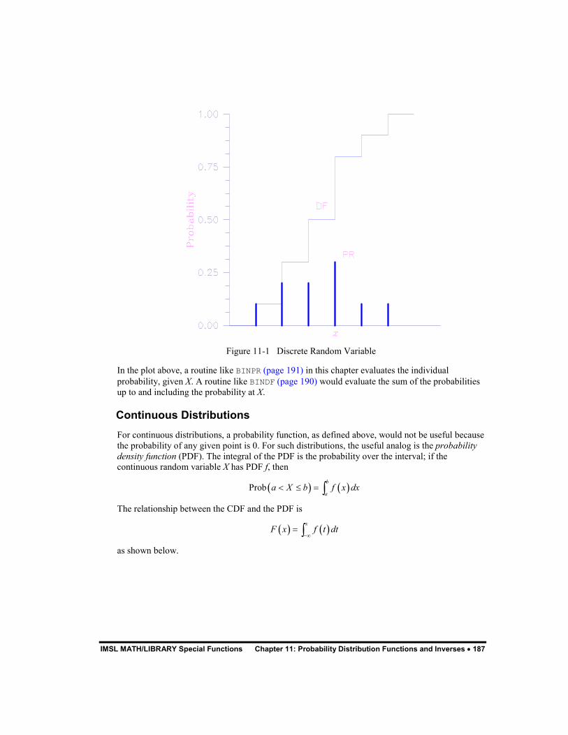
IMSL MATH/LIBRARY Special Functions Chapter 11: Probability Distribution Functions and Inverses � 187
Figure 11-1 Discrete Random Variable
In the plot above, a routine like BINPR (page 191) in this chapter evaluates the individual probability, given X. A routine like BINDF (page 190) would evaluate the sum of the probabilities up to and including the probability at X.
Continuous Distributions For continuous distributions, a probability function, as defined above, would not be useful because the probability of any given point is 0. For such distributions, the useful analog is the probability density function (PDF). The integral of the PDF is the probability over the interval; if the continuous random variable X has PDF f, then
� � � �Probb
aa X b f x dx� � � �
The relationship between the CDF and the PDF is
� � � �x
F x f t dt��
� �
as shown below.
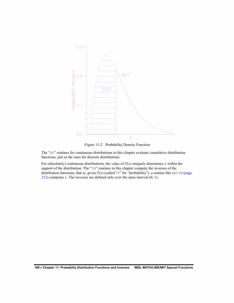
188 � Chapter 11: Probability Distribution Functions and Inverses IMSL MATH/LIBRARY Special Functions
Figure 11-2 Probability Density Function
The “DF” routines for continuous distributions in this chapter evaluate cumulative distribution functions, just as the ones for discrete distributions.
For (absolutely) continuous distributions, the value of F(x) uniquely determines x within the support of the distribution. The “IN” routines in this chapter compute the inverses of the distribution functions; that is, given F(x) (called “P” for “probability”), a routine like BETIN (page 212) computes x. The inverses are defined only over the open interval (0, 1).
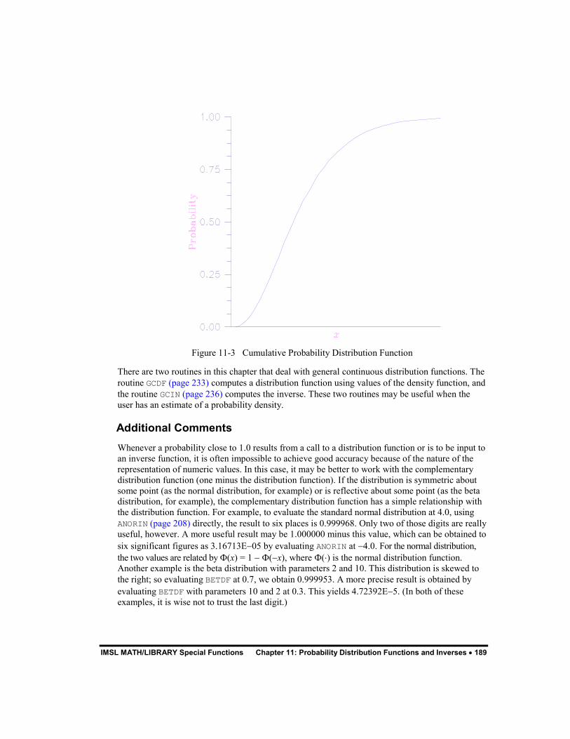
IMSL MATH/LIBRARY Special Functions Chapter 11: Probability Distribution Functions and Inverses � 189
Figure 11-3 Cumulative Probability Distribution Function
There are two routines in this chapter that deal with general continuous distribution functions. The routine GCDF (page 233) computes a distribution function using values of the density function, and the routine GCIN (page 236) computes the inverse. These two routines may be useful when the user has an estimate of a probability density.
Additional Comments Whenever a probability close to 1.0 results from a call to a distribution function or is to be input to an inverse function, it is often impossible to achieve good accuracy because of the nature of the representation of numeric values. In this case, it may be better to work with the complementary distribution function (one minus the distribution function). If the distribution is symmetric about some point (as the normal distribution, for example) or is reflective about some point (as the beta distribution, for example), the complementary distribution function has a simple relationship with the distribution function. For example, to evaluate the standard normal distribution at 4.0, using ANORIN (page 208) directly, the result to six places is 0.999968. Only two of those digits are really useful, however. A more useful result may be 1.000000 minus this value, which can be obtained to six significant figures as 3.16713E�05 by evaluating ANORIN at �4.0. For the normal distribution, the two values are related by �(x) = 1 � �(�x), where �(�) is the normal distribution function. Another example is the beta distribution with parameters 2 and 10. This distribution is skewed to the right; so evaluating BETDF at 0.7, we obtain 0.999953. A more precise result is obtained by evaluating BETDF with parameters 10 and 2 at 0.3. This yields 4.72392E�5. (In both of these examples, it is wise not to trust the last digit.)
190 � Chapter 11: Probability Distribution Functions and Inverses IMSL MATH/LIBRARY Special Functions
Many of the algorithms used by routines in this chapter are discussed by Abramowitz and Stegun (1964). The algorithms make use of various expansions and recursive relationships, and often use different methods in different regions.
Cumulative distribution functions are defined for all real arguments; however, if the input to one of the distribution functions in this chapter is outside the range of the random variable, an error of Type 1 is issued, and the output is set to zero or one, as appropriate. A Type 1 error is of lowest severity, a “note;” and, by default, no printing or stopping of the program occurs. The other common errors that occur in the routines of this chapter are Type 2, “alert,” for a function value being set to zero due to underflow; Type 3, “warning,” for considerable loss of accuracy in the result returned; and Type 5, “terminal,” for incorrect and/ or inconsistent input, complete loss of accuracy in the result returned, or inability to represent the result (because of overflow). When a Type 5 error occurs, the result is set to NaN (not a number, also used as a missing value code, obtained by IMSL routine AMACH(6). (See the section “User Errors” in the Reference Material.)
BINDF This function evaluates the binomial distribution function.
Function Return Value BINDF — Function value, the probability that a binomial random variable takes a value less
than or equal to K. (Output) BINDF is the probability that K or fewer successes occur in N independent Bernoulli trials, each of which has a P probability of success.
Required Arguments K — Argument for which the binomial distribution function is to be evaluated. (Input)
N — Number of Bernoulli trials. (Input)
P — Probability of success on each trial. (Input)
FORTRAN 90 Interface Generic: BINDF (K, N, P)
Specific: The specific interface names are S_BINDF and D_BINDF.
FORTRAN 77 Interface Single: BINDF (K, N, P)
Double: The double precision function name is DBINDF.
IMSL MATH/LIBRARY Special Functions Chapter 11: Probability Distribution Functions and Inverses � 191
Example Suppose X is a binomial random variable with n = 5 and p = 0.95. In this example, we find the probability that X is less than or equal to 3.
USE IMSL_LIBRARIES INTEGER K, N, NOUT REAL P, PR ! CALL UMACH (2, NOUT) K = 3 N = 5 P = 0.95 PR = BINDF(K,N,P) WRITE (NOUT,99999) PR 99999 FORMAT (’ The probability that X is less than or equal to 3 is ’ & , F6.4) END
Output The probability that X is less than or equal to 3 is 0.0226
Comments Informational errors Type Code
1 3 The input argument, K, is less than zero. 1 4 The input argument, K, is greater than the number of Bernoulli
trials, N.
Description Function BINDF evaluates the distribution function of a binomial random variable with parameters n and p. It does this by summing probabilities of the random variable taking on the specific values in its range. These probabilities are computed by the recursive relationship
� �� �
� �� �
1Pr Pr 1
1n j p
X j X jj p� �
� � � �
�
To avoid the possibility of underflow, the probabilities are computed forward from 0, if k is not greater than n times p, and are computed backward from n, otherwise. The smallest positive machine number, �, is used as the starting value for summing the probabilities, which are rescaled by (1 � p)n� if forward computation is performed and by pn� if backward computation is done.
For the special case of p = 0, BINDF is set to 1; and for the case p = 1, BINDF is set to 1 if k = n and to 0 otherwise.
BINPR This function evaluates the binomial probability function.
192 � Chapter 11: Probability Distribution Functions and Inverses IMSL MATH/LIBRARY Special Functions
Function Return Value BINPR — Function value, the probability that a binomial random variable takes a value equal
to K. (Output)
Required Arguments K — Argument for which the binomial probability function is to be evaluated. (Input)
N — Number of Bernoulli trials. (Input)
P — Probability of success on each trial. (Input)
FORTRAN 90 Interface Generic: BINPR (K, N, P)
Specific: The specific interface names are S_BINPR and D_BINPR.
FORTRAN 77 Interface Single: BINPR (K, N, P)
Double: The double precision function name is DBINPR.
Example Suppose X is a binomial random variable with n = 5 and p = 0.95. In this example, we find the probability that X is equal to 3.
USE IMSL_LIBRARIES INTEGER K, N, NOUT REAL P, PR ! CALL UMACH (2, NOUT) K = 3 N = 5 P = 0.95 PR = BINPR(K,N,P) WRITE (NOUT,99999) PR 99999 FORMAT (’ The probability that X is equal to 3 is ’, F6.4) END
Output The probability that X is equal to 3 is 0.0214
Comments Informational errors Type Code
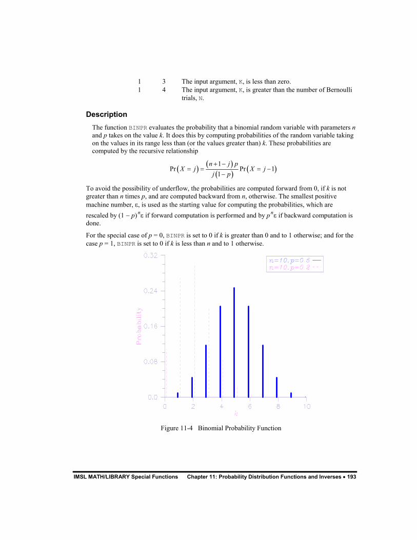
IMSL MATH/LIBRARY Special Functions Chapter 11: Probability Distribution Functions and Inverses � 193
1 3 The input argument, K, is less than zero. 1 4 The input argument, K, is greater than the number of Bernoulli
trials, N.
Description The function BINPR evaluates the probability that a binomial random variable with parameters n and p takes on the value k. It does this by computing probabilities of the random variable taking on the values in its range less than (or the values greater than) k. These probabilities are computed by the recursive relationship
� �� �
� �� �
1Pr Pr 1
1n j p
X j X jj p� �
� � � �
�
To avoid the possibility of underflow, the probabilities are computed forward from 0, if k is not greater than n times p, and are computed backward from n, otherwise. The smallest positive machine number, �, is used as the starting value for computing the probabilities, which are rescaled by (1 � p)n� if forward computation is performed and by pn� if backward computation is done.
For the special case of p = 0, BINPR is set to 0 if k is greater than 0 and to 1 otherwise; and for the case p = 1, BINPR is set to 0 if k is less than n and to 1 otherwise.
Figure 11-4 Binomial Probability Function

194 � Chapter 11: Probability Distribution Functions and Inverses IMSL MATH/LIBRARY Special Functions
HYPDF This function evaluates the hypergeometric distribution function.
Function Return Value HYPDF — Function value, the probability that a hypergeometric random variable takes a
value less than or equal to K. (Output) HYPDF is the probability that K or fewer defectives occur in a sample of size N drawn from a lot of size L that contains M defectives. See Comment 1.
Required Arguments K — Argument for which the hypergeometric distribution function is to be evaluated. (Input)
N — Sample size. (Input) N must be greater than zero and greater than or equal to K.
M — Number of defectives in the lot. (Input)
L — Lot size. (Input) L must be greater than or equal to N and M.
FORTRAN 90 Interface Generic: HYPDF (K, N, M, L )
Specific: The specific interface names are S_HYPDF and D_HYPDF.
FORTRAN 77 Interface Single: HYPDF (K, N, M, L)
Double: The double precision function name is DHYPDF.
Example Suppose X is a hypergeometric random variable with n = 100, l = 1000, and m = 70. In this example, we evaluate the distribution function at 7.
USE IMSL_LIBRARIES INTEGER K, L, M, N, NOUT REAL DF ! CALL UMACH (2, NOUT) K = 7 N = 100 L = 1000
IMSL MATH/LIBRARY Special Functions Chapter 11: Probability Distribution Functions and Inverses � 195
M = 70 DF = HYPDF(K,N,M,L) WRITE (NOUT,99999) DF 99999 FORMAT (’ The probability that X is less than or equal to 7 is ’ & , F6.4) END
Output The probability that X is less than or equal to 7 is 0.5995
Comments 1. If the generic version of this function is used, the immediate result must be stored in a
variable before use in an expression. For example:
X = HYPDF(K, N, M, L) Y = SQRT(X) must be used rather than
Y = SQRT(HYPDF(K, N, M, L))
If this is too much of a restriction on the programmer, then the specific name can be used without this restriction.
2. Informational errors
Type Code
1 5 The input argument, K, is less than zero. 1 6 The input argument, K, is greater than the sample size.
Description The function HYPDF evaluates the distribution function of a hypergeometric random variable with parameters n, l, and m. The hypergeometric random variable X can be thought of as the number of items of a given type in a random sample of size n that is drawn without replacement from a population of size l containing m items of this type. The probability function is
� � � �Pr for , 1, 2, , min ,m l mj n j
ln
X j j i i i n m�� �� �
� �� ��� �� �
� �� �� �
� � � � � �
where i = max(0, n � l + m).
If k is greater than or equal to i and less than or equal to min(n, m), HYPDF sums the terms in this expression for j going from i up to k. Otherwise, HYPDF returns 0 or 1, as appropriate. So, as to avoid rounding in the accumulation, HYPDF performs the summation differently depending on whether or not k is greater than the mode of the distribution, which is the greatest integer in (m + 1)(n + 1)/(l + 2).
196 � Chapter 11: Probability Distribution Functions and Inverses IMSL MATH/LIBRARY Special Functions
HYPPR This function evaluates the hypergeometric probability function.
Function Return Value HYPPR — Function value, the probability that a hypergeometric random variable takes a
value equal to K. (Output) HYPPR is the probability that exactly K defectives occur in a sample of size N drawn from a lot of size L that contains M defectives. See Comment 1.
Required Arguments K — Argument for which the hypergeometric probability function is to be evaluated. (Input)
N — Sample size. (Input) N must be greater than zero and greater than or equal to K.
M — Number of defectives in the lot. (Input)
L — Lot size. (Input) L must be greater than or equal to N and M.
FORTRAN 90 Interface Generic: HYPPR (K, N, M, L)
Specific: The specific interface names are S_HYPPR and D_HYPPR.
FORTRAN 77 Interface Single: HYPPR (K, N, M, L)
Double: The double precision function name is DHYPPR.
Example Suppose X is a hypergeometric random variable with n = 100, l = 1000, and m = 70. In this example, we evaluate the probability function at 7.
USE IMSL_LIBRARIES INTEGER K, L, M, N, NOUT REAL PR ! CALL UMACH (2, NOUT) K = 7 N = 100 L = 1000
IMSL MATH/LIBRARY Special Functions Chapter 11: Probability Distribution Functions and Inverses � 197
M = 70 PR = HYPPR(K,N,M,L) WRITE (NOUT,99999) PR 99999 FORMAT (’ The probability that X is equal to 7 is ’, F6.4) END
Output The probability that X is equal to 7 is 0.1628
Comments 1. If the generic version of this function is used, the immediate result must be stored in a
variable before use in an expression. For example:
X = HYPPR(K, N, M, L) Y = SQRT(X) must be used rather than
Y = SQRT(HYPPR(K, N, M, L))
If this is too much of a restriction on the programmer, then the specific name can be used without this restriction.
2. Informational errors Type Code
1 5 The input argument, K, is less than zero. 1 6 The input argument, K, is greater than the sample size.
Description The function HYPPR evaluates the probability function of a hypergeometric random variable with parameters n, l, and m. The hypergeometric random variable X can be thought of as the number of items of a given type in a random sample of size n that is drawn without replacement from a population of size l containing m items of this type. The probability function is
� � � �Pr for , 1, 2, min ,m l mk n k
ln
X k k i i i n m�� �� �
� �� ��� �� �
� �� �� �
� � � � � �
where i = max(0, n � l + m).
HYPPR evaluates the expression using log gamma functions.
POIDF This function evaluates the Poisson distribution function.
198 � Chapter 11: Probability Distribution Functions and Inverses IMSL MATH/LIBRARY Special Functions
Function Return Value POIDF — Function value, the probability that a Poisson random variable takes a value less
than or equal to K. (Output)
Required Arguments K — Argument for which the Poisson distribution function is to be evaluated. (Input)
THETA — Mean of the Poisson distribution. (Input) THETA must be positive.
FORTRAN 90 Interface Generic: POIDF (K, THETA)
Specific: The specific interface names are S_POIDF and D_POIDF.
FORTRAN 77 Interface Single: POIDF (K, THETA)
Double: The double precision function name is DPOIDF.
Example Suppose X is a Poisson random variable with � = 10. In this example, we evaluate the distribution function at 7.
USE IMSL_LIBRARIES INTEGER K, NOUT REAL DF, THETA ! CALL UMACH (2, NOUT) K = 7 THETA = 10.0 DF = POIDF(K,THETA) WRITE (NOUT,99999) DF 99999 FORMAT (’ The probability that X is less than or equal to ’, & ’7 is ’, F6.4) END
Output The probability that X is less than or equal to 7 is 0.2202
Comments Informational error Type Code
1 1 The input argument, K, is less than zero.
IMSL MATH/LIBRARY Special Functions Chapter 11: Probability Distribution Functions and Inverses � 199
Description The function POIDF evaluates the distribution function of a Poisson random variable with parameter THETA. THETA, which is the mean of the Poisson random variable, must be positive. The probability function (with � = THETA) is
f(x) = e�� �x/x!, for x = 0, 1, 2, �
The individual terms are calculated from the tails of the distribution to the mode of the distribution and summed. POIDF uses the recursive relationship
f(x + 1) = f(x)�/(x + 1), for x = 0, 1, 2, �, k � 1
with f(0) = e��.
POIPR This function evaluates the Poisson probability function.
Function Return Value POIPR — Function value, the probability that a Poisson random variable takes a value equal
to K. (Output)
Required Arguments K — Argument for which the Poisson distribution function is to be evaluated. (Input)
THETA — Mean of the Poisson distribution. (Input) THETA must be positive.
FORTRAN 90 Interface Generic: POIPR(K, THETA)
Specific: The specific interface names are S_POIPR and D_POIPR.
FORTRAN 77 Interface Single: POIPR(K, THETA)
Double: The double precision function name is DPOIPR.
Example Suppose X is a Poisson random variable with � = 10. In this example, we evaluate the probability function at 7.
200 � Chapter 11: Probability Distribution Functions and Inverses IMSL MATH/LIBRARY Special Functions
USE POIPR_INT USE UMACH_INT INTEGER K, NOUT REAL PR, THETA ! CALL UMACH (2, NOUT) K = 7 THETA = 10.0 PR = POIPR(K,THETA) WRITE (NOUT,99999) PR 99999 FORMAT (’ The probability that X is equal to 7 is ’, F6.4) END
Output The probability that X is equal to 7 is 0.0901
Comments Informational error Type Code
1 1 The input argument, K, is less than zero.
Description The function POIPR evaluates the probability function of a Poisson random variable with parameter THETA. THETA, which is the mean of the Poisson random variable, must be positive. The probability function (with � = THETA) is
f(k) = e���k/k!, for k = 0, 1, 2, �
POIPR evaluates this function directly, taking logarithms and using the log gamma function.
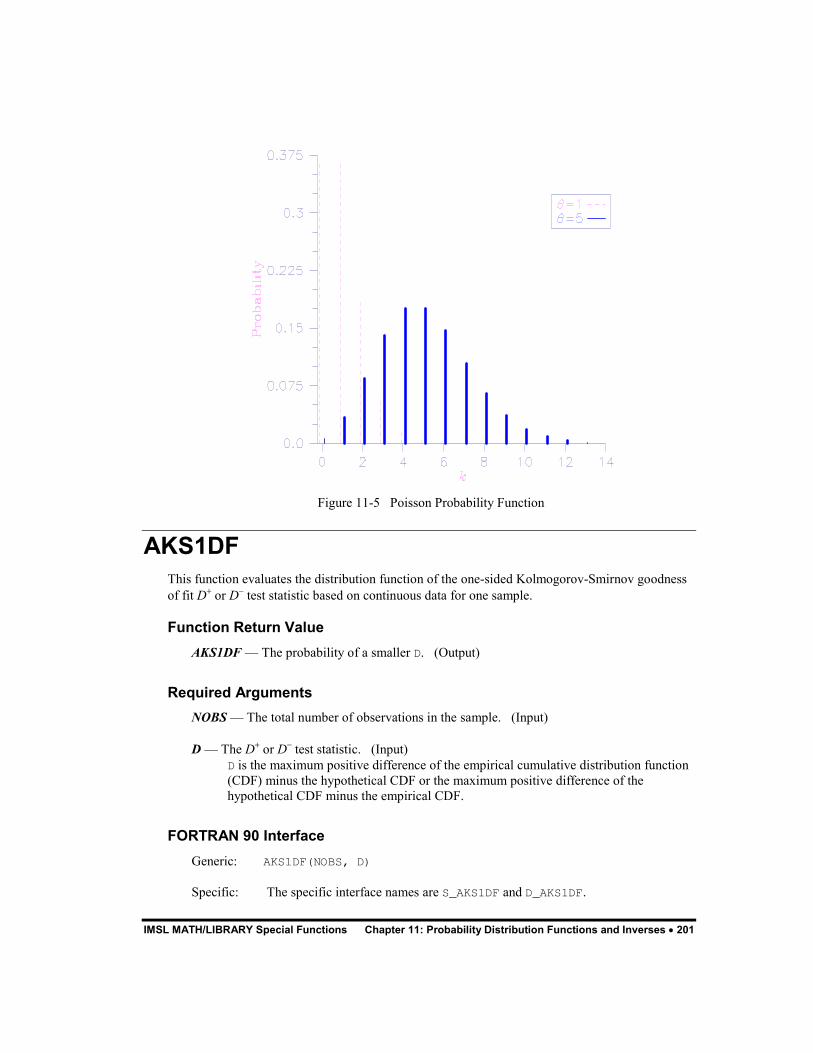
IMSL MATH/LIBRARY Special Functions Chapter 11: Probability Distribution Functions and Inverses � 201
Figure 11-5 Poisson Probability Function
AKS1DF This function evaluates the distribution function of the one-sided Kolmogorov-Smirnov goodness of fit D� or D� test statistic based on continuous data for one sample.
Function Return Value AKS1DF — The probability of a smaller D. (Output)
Required Arguments NOBS — The total number of observations in the sample. (Input)
D — The D� or D� test statistic. (Input) D is the maximum positive difference of the empirical cumulative distribution function (CDF) minus the hypothetical CDF or the maximum positive difference of the hypothetical CDF minus the empirical CDF.
FORTRAN 90 Interface Generic: AKS1DF(NOBS, D)
Specific: The specific interface names are S_AKS1DF and D_AKS1DF.

202 � Chapter 11: Probability Distribution Functions and Inverses IMSL MATH/LIBRARY Special Functions
FORTRAN 77 Interface Single: AKS1DF(NOBS, D)
Double: The double precision function name is DKS1DF.
Example In this example, the exact one-sided probabilities for the tabled values of D+ or D�, given, for example, in Conover (1980, page 462), are computed. Tabled values at the 10% level of significance are used as input to AKS1DF for sample sizes of 5 to 50 in increments of 5. The last two tabled values are obtained using the asymptotic critical values of
1.07 / NOBS
The resulting probabilities should all be close to 0.90. USE AKS1DF_INT USE UMACH_INT INTEGER I, NOBS, NOUT REAL D(10) ! DATA D/0.447, 0.323, 0.266, 0.232, 0.208, 0.190, 0.177, 0.165, & 0.160, 0.151/ ! CALL UMACH (2, NOUT) ! DO 10 I=1, 10 NOBS = 5*I ! WRITE (NOUT,99999) D(I), NOBS, AKS1DF(NOBS,D(I)) ! 99999 FORMAT (’ One-sided Probability for D = ’, F8.3, ’ with NOBS ’ & , ’= ’, I2, ’ is ’, F8.4) 10 CONTINUE END
Output One-sided Probability for D = 0.447 with NOBS = 5 is 0.9000 One-sided Probability for D = 0.323 with NOBS = 10 is 0.9006 One-sided Probability for D = 0.266 with NOBS = 15 is 0.9002 One-sided Probability for D = 0.232 with NOBS = 20 is 0.9009 One-sided Probability for D = 0.208 with NOBS = 25 is 0.9002 One-sided Probability for D = 0.190 with NOBS = 30 is 0.8992 One-sided Probability for D = 0.177 with NOBS = 35 is 0.9011 One-sided Probability for D = 0.165 with NOBS = 40 is 0.8987 One-sided Probability for D = 0.160 with NOBS = 45 is 0.9105 One-sided Probability for D = 0.151 with NOBS = 50 is 0.9077
Comments 1. Workspace may be explicitly provided, if desired, by use of AK21DF/DK21DF. The
reference is:
IMSL MATH/LIBRARY Special Functions Chapter 11: Probability Distribution Functions and Inverses � 203
AK2DF(NOBS, D, WK)
The additional argument is:
WK — Work vector of length 3 * NOBS + 3 if NOBS � 80. WK is not used if NOBS is greater than 80.
2. Informational errors Type Code
1 2 Since the D test statistic is less than zero, the distribution function is zero at D.
1 3 Since the D test statistic is greater than one, the distribution function is one at D.
3. If NOBS � 80, then exact one-sided probabilities are computed. In this case, on the order of NOBS� operations are required. For NOBS > 80, approximate one-sided probabilities are computed. These approximate probabilities require very few computations.
4. An approximate two-sided probability for the D = max (D�, D��) statistic can be computed as twice the AKS1DF probability for D (minus one, if the probability from AKS1DF is greater than 0.5).
Description Routine AKS1DF computes the cumulative distribution function (CDF) for the one-sided Kolmogorov-Smirnov one-sample D� or D� statistic when the theoretical CDF is strictly continuous. Exact probabilities are computed according to a method given by Conover (1980, page 350) for sample sizes of 80 or less. For sample sizes greater than 80, the asympotic methods discussed by Conover are used.
Let F(x) denote the theoretical distribution function, and let Sn(x) denote the empirical distribution function obtained from a sample of size NOBS. Then, the D� statistic is computed as
� � � �sup nx
D F x S x� � �� �� �
while the one-sided D� statistic is computed as
� � � �sup nx
D S x F x� � �� �� �
Programming Notes Routine AKS1DF requires on the order of NOBS� operations to compute the exact probabilities, where an operation consists of taking ten or so logarithms. Because so much computation is occurring within each “operation,” AKS1DF is much slower than its two-sample counterpart, IMSL function AKS2DF (page 204).
204 � Chapter 11: Probability Distribution Functions and Inverses IMSL MATH/LIBRARY Special Functions
AKS2DF This function evaluates the distribution function of the Kolmogorov-Smirnov goodness of fit D test statistic based on continuous data for two samples.
Function Return Value AKS2DF — The probability of a smaller D. (Output)
Required Arguments NOBSX — The total number of observations in the first sample. (Input)
NOBSY — The total number of observations in the second sample. (Input)
D — The D test statistic. (Input) D is the maximum absolute difference between empirical cumulative distribution functions (CDFs) of the two samples.
FORTRAN 90 Interface Generic: AKS2DF(NOBSX, NOBSY, D)
Specific: The specific interface names are S_AKS2DF and D_AKS2DF.
FORTRAN 77 Interface Single: AKS2DF(NOBSX, NOBSY, D)
Double: The double precision function name is DKS2DF.
Example Function AKS2DF is used to compute the probability of a smaller D statistic for a variety of sample sizes using values close to the 0.95 probability value.
USE AKS2DF_INT USE UMACH_INT INTEGER I, NOBSX(10), NOBSY(10), NOUT REAL D(10) ! DATA NOBSX/5, 20, 40, 70, 110, 200, 200, 200, 100, 100/ DATA NOBSY/10, 10, 10, 10, 10, 20, 40, 60, 80, 100/ DATA D/0.7, 0.55, 0.475, 0.4429, 0.4029, 0.2861, 0.2113, 0.1796, & 0.18, 0.18/ ! CALL UMACH (2, NOUT) ! DO 10 I=1, 10 !
IMSL MATH/LIBRARY Special Functions Chapter 11: Probability Distribution Functions and Inverses � 205
WRITE (NOUT,99999) D(I), NOBSX(I), NOBSY(I), & AKS2DF(NOBSX(I),NOBSY(I),D(I)) ! 99999 FORMAT (’ Probability for D = ’, F5.3, ’ with NOBSX = ’, I3, & ’ and NOBSY = ’, I3, ’ is ’, F9.6, ’.’) 10 CONTINUE END
Output Probability for D = 0.700 with NOBSX = 5 and NOBSY = 10 is 0.980686. Probability for D = 0.550 with NOBSX = 20 and NOBSY = 10 is 0.987553. Probability for D = 0.475 with NOBSX = 40 and NOBSY = 10 is 0.972423. Probability for D = 0.443 with NOBSX = 70 and NOBSY = 10 is 0.961646. Probability for D = 0.403 with NOBSX = 110 and NOBSY = 10 is 0.928667. Probability for D = 0.286 with NOBSX = 200 and NOBSY = 20 is 0.921126. Probability for D = 0.211 with NOBSX = 200 and NOBSY = 40 is 0.917110. Probability for D = 0.180 with NOBSX = 200 and NOBSY = 60 is 0.914520. Probability for D = 0.180 with NOBSX = 100 and NOBSY = 80 is 0.908185. Probability for D = 0.180 with NOBSX = 100 and NOBSY = 100 is 0.946098.
Comments 1. Workspace may be explicitly provided, if desired, by use of AK22DF/DK22DF. The
reference is:
AK22DF(NOBSX, NOBSY, D, WK)
The additional argument is
WK — Work vector of length max(NOBSX, NOBSY) + 1.
2. Informational errors Type Code
1 2 Since the D test statistic is less than zero, then the distribution function is zero at D.
1 3 Since the D test statistic is greater than one, then the distribution function is one at D.
Description Function AKS2DF computes the cumulative distribution function (CDF) for the two-sided Kolmogorov-Smirnov two-sample D statistic when the theoretical CDF is strictly continuous. Exact probabilities are computed according to a method given by Kim and Jennrich (1973). Approximate asymptotic probabilities are computed according to methods also given in this reference.
Let Fn(x) and Gm(x) denote the empirical distribution functions for the two samples, based on n = NOBSX and m = NOBSY observations. Then, the D statistic is computed as
� � � �sup n mx
D F x G x� �

206 � Chapter 11: Probability Distribution Functions and Inverses IMSL MATH/LIBRARY Special Functions
Programming Notes Function AKS2DF requires on the order of NOBSX * NOBSY operations to compute the exact probabilities, where an operation consists of an addition and a multiplication. For NOBSX * NOBSY less than 10000, the exact probability is computed. If this is not the case, then the Smirnov approximation discussed by Kim and Jennrich is used if the minimum of NOBSX and NOBSY is greater than ten percent of the maximum of NOBSX and NOBSY, or if the minimum is greater than 80. Otherwise, the Kolmogorov approximation discussed by Kim and Jennrich is used.
ANORDF This function evaluates the standard normal (Gaussian) distribution function.
Function Return Value ANORDF — Function value, the probability that a normal random variable takes a value less
than or equal to X. (Output)
Required Arguments X — Argument for which the normal distribution function is to be evaluated. (Input)
FORTRAN 90 Interface Generic: ANORDF (X)
Specific: The specific interface names are S_ANORDF and D_ANORDF.
FORTRAN 77 Interface Single: ANORDF (X)
Double: The double precision function name is DNORDF.
Example Suppose X is a normal random variable with mean 100 and variance 225. In this example, we find the probability that X is less than 90, and the probability that X is between 105 and 110.
USE ANORDF_INT USE UMACH_INT INTEGER NOUT REAL P, X1, X2 ! CALL UMACH (2, NOUT) X1 = (90.0-100.0)/15.0 P = ANORDF(X1) WRITE (NOUT,99998) P 99998 FORMAT (’ The probability that X is less than 90 is ’, F6.4)

IMSL MATH/LIBRARY Special Functions Chapter 11: Probability Distribution Functions and Inverses � 207
X1 = (105.0-100.0)/15.0 X2 = (110.0-100.0)/15.0 P = ANORDF(X2) - ANORDF(X1) WRITE (NOUT,99999) P 99999 FORMAT (’ The probability that X is between 105 and 110 is ’, & F6.4) END
Output The probability that X is less than 90 is 0.2525 The probability that X is between 105 and 110 is 0.1169
Description Function ANORDF evaluates the distribution function, �, of a standard normal (Gaussian) random variable, that is,
� �2 / 21
2
x tx e dt�
�
��
� � �
The value of the distribution function at the point x is the probability that the random variable takes a value less than or equal to x.
The standard normal distribution (for which ANORDF is the distribution function) has mean of 0 and variance of 1. The probability that a normal random variable with mean � and variance � is less than y is given by ANORDF evaluated at (y � �)/.
�(x) is evaluated by use of the complementary error function, erfc. (See ERFC in Chapter 5, “Error Funtions and Related Functions” of this manual.)) The relationship is:
� � � �erfc / 2.0 / 2x x� � �
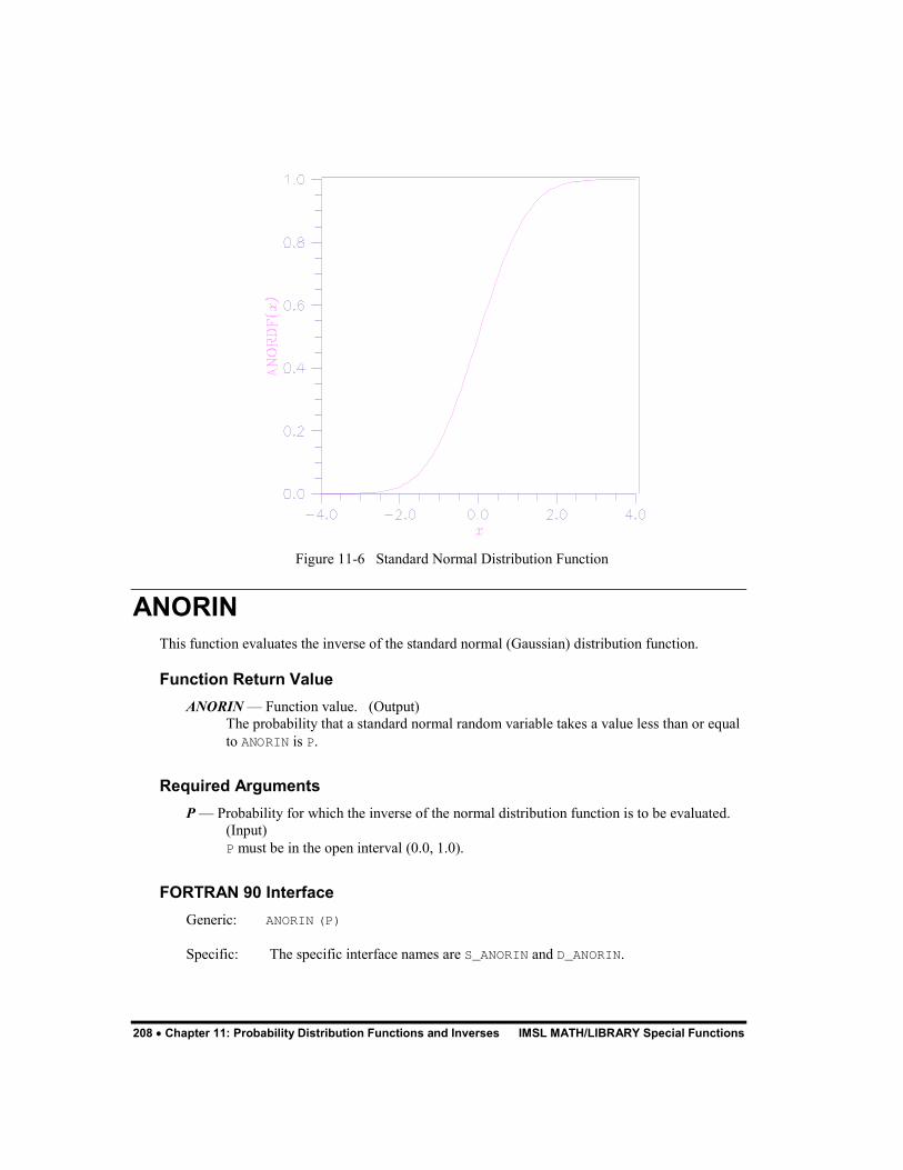
208 � Chapter 11: Probability Distribution Functions and Inverses IMSL MATH/LIBRARY Special Functions
Figure 11-6 Standard Normal Distribution Function
ANORIN This function evaluates the inverse of the standard normal (Gaussian) distribution function.
Function Return Value ANORIN — Function value. (Output)
The probability that a standard normal random variable takes a value less than or equal to ANORIN is P.
Required Arguments P — Probability for which the inverse of the normal distribution function is to be evaluated.
(Input) P must be in the open interval (0.0, 1.0).
FORTRAN 90 Interface Generic: ANORIN (P)
Specific: The specific interface names are S_ANORIN and D_ANORIN.
IMSL MATH/LIBRARY Special Functions Chapter 11: Probability Distribution Functions and Inverses � 209
FORTRAN 77 Interface Single: ANORIN (P)
Double: The double precision function name is DNORIN.
Example In this example, we compute the point such that the probability is 0.9 that a standard normal random variable is less than or equal to this point.
USE ANORIN_INT USE UMACH_INT INTEGER NOUT REAL P, X ! CALL UMACH (2, NOUT) P = 0.9 X = ANORIN(P) WRITE (NOUT,99999) X 99999 FORMAT (’ The 90th percentile of a standard normal is ’, F6.4) END
Output The 90th percentile of a standard normal is 1.2816
Description Function ANORIN evaluates the inverse of the distribution function, �, of a standard normal (Gaussian) random variable, that is, ANORIN(P) = ���(p), where
� �2 / 21
2
x tx e dt�
�
��
� � �
The value of the distribution function at the point x is the probability that the random variable takes a value less than or equal to x. The standard normal distribution has a mean of 0 and a variance of 1.
References used to design this routine include Hart et al. (1968), Kinnucan and Kuki (1968), and Strecok (1968).
BETDF This function evaluates the beta probability distribution function.
Function Return Value BETDF — Probability that a random variable from a beta distribution having parameters PIN
and QIN will be less than or equal to X. (Output)
210 � Chapter 11: Probability Distribution Functions and Inverses IMSL MATH/LIBRARY Special Functions
Required Arguments X — Argument for which the beta distribution function is to be evaluated. (Input)
PIN — First beta distribution parameter. (Input) PIN must be positive.
QIN — Second beta distribution parameter. (Input) QIN must be positive.
FORTRAN 90 Interface Generic: BETDF(X, PIN, QIN)
Specific: The specific interface names are S_BETDF and D_BETDF.
FORTRAN 77 Interface Single: BETDF(X, PIN, QIN)
Double: The double precision function name is DBETDF.
Example Suppose X is a beta random variable with parameters 12 and 12. (X has a symmetric distribution.) In this example, we find the probability that X is less than 0.6 and the probability that X is between 0.5 and 0.6. (Since X is a symmetric beta random variable, the probability that it is less than 0.5 is 0.5.)
USE BETDF_INT USE UMACH_INT INTEGER NOUT REAL P, PIN, QIN, X ! CALL UMACH (2, NOUT) PIN = 12.0 QIN = 12.0 X = 0.6 P = BETDF(X,PIN,QIN) WRITE (NOUT,99998) P 99998 FORMAT (’ The probability that X is less than 0.6 is ’, F6.4) X = 0.5 P = P - BETDF(X,PIN,QIN) WRITE (NOUT,99999) P 99999 FORMAT (’ The probability that X is between 0.5 and 0.6 is ’, & F6.4) END
Output The probability that X is less than 0.6 is 0.8364 The probability that X is between 0.5 and 0.6 is 0.3364
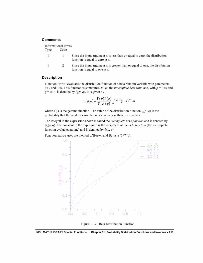
IMSL MATH/LIBRARY Special Functions Chapter 11: Probability Distribution Functions and Inverses � 211
Comments Informational errors Type Code
1 1 Since the input argument X is less than or equal to zero, the distribution function is equal to zero at X.
1 2 Since the input argument X is greater than or equal to one, the distribution function is equal to one at X.
Description Function BETDF evaluates the distribution function of a beta random variable with parameters PIN and QIN. This function is sometimes called the incomplete beta ratio and, with p = PIN and q = QIN, is denoted by Ix(p, q). It is given by
� �� � � �
� �� �
11
0, 1
x qpx
p qI p q t t dt
p q�
�
� �� �
� ��
where (�) is the gamma function. The value of the distribution function Ix(p, q) is the probability that the random variable takes a value less than or equal to x.
The integral in the expression above is called the incomplete beta function and is denoted by �x(p, q). The constant in the expression is the reciprocal of the beta function (the incomplete function evaluated at one) and is denoted by �(p, q).
Function BETDF uses the method of Bosten and Battiste (1974b).
Figure 11-7 Beta Distribution Function
212 � Chapter 11: Probability Distribution Functions and Inverses IMSL MATH/LIBRARY Special Functions
BETIN This function evaluates the inverse of the beta distribution function.
Function Return Value BETIN — Function value. (Output)
The probability that a beta random variable takes a value less than or equal to BETIN is P.
Required Arguments P — Probability for which the inverse of the beta distribution function is to be evaluated.
(Input) P must be in the open interval (0.0, 1.0).
PIN — First beta distribution parameter. (Input) PIN must be positive.
QIN — Second beta distribution parameter. (Input) QIN must be positive.
FORTRAN 90 Interface Generic: BETIN(P, PIN, QIN)
Specific: The specific interface names are S_BETIN and D_BETIN.
FORTRAN 77 Interface Single: BETIN(P, PIN, QIN)
Double: The double precision function name is DBETIN.
Example Suppose X is a beta random variable with parameters 12 and 12. (X has a symmetric distribution.) In this example, we find the value x� such that the probability that X � x� is 0.9.
USE BETIN_INT USE UMACH_INT INTEGER NOUT REAL P, PIN, QIN, X ! CALL UMACH (2, NOUT) PIN = 12.0 QIN = 12.0 P = 0.9 X = BETIN(P,PIN,QIN)
IMSL MATH/LIBRARY Special Functions Chapter 11: Probability Distribution Functions and Inverses � 213
WRITE (NOUT,99999) X 99999 FORMAT (’ X is less than ’, F6.4, ’ with probability 0.9.’) END
Output X is less than 0.6299 with probability 0.9.
Comments Informational error Type Code
3 1 The value for the inverse Beta distribution could not be found in 100 iterations. The best approximation is used.
Description The function BETIN evaluates the inverse distribution function of a beta random variable with parameters PIN and QIN, that is, with P = P, p = PIN, and q = QIN; it determines x (= BETIN(P, PIN, QIN) ), such that
� � � �
� �� �
11
0 = 1
x qpp qP t t dt
p q�
�
� ��
� ��
where (�) is the gamma function. The probability that the random variable takes a value less than or equal to x is P.
BNRDF This function evaluates the bivariate normal distribution function.
Function Return Value BNRDF — Function value, the probability that a bivariate normal random variable with
correlation RHO takes a value less than or equal to X and less than or equal to Y. (Output)
Required Arguments X — One argument for which the bivariate normal distribution function is to be evaluated.
(Input)
Y — The other argument for which the bivariate normal distribution function is to be evaluated. (Input)
RHO — Correlation coefficient. (Input)
FORTRAN 90 Interface Generic: BNRDF(X, Y, RHO)
214 � Chapter 11: Probability Distribution Functions and Inverses IMSL MATH/LIBRARY Special Functions
Specific: The specific interface names are S_BNRDF and D_BNRDF.
FORTRAN 77 Interface Single: BNRDF(X, Y, RHO)
Double: The double precision function name is DBNRDF.
Example Suppose (X, Y) is a bivariate normal random variable with mean (0, 0) and variance-covariance matrix
1.0 0.90.9 1.0
� �� �� �
In this example, we find the probability that X is less than �2.0 and Y is less than 0.0. USE BNRDF_INT USE UMACH_INT INTEGER NOUT REAL P, RHO, X, Y ! CALL UMACH (2, NOUT) X = -2.0 Y = 0.0 RHO = 0.9 P = BNRDF(X,Y,RHO) WRITE (NOUT,99999) P 99999 FORMAT (’ The probability that X is less than -2.0 and Y ’, & ’is less than 0.0 is ’, F6.4) END
Output The probability that X is less than -2.0 and Y is less than 0.0 is 0.0228
Description Function BNRDF evaluates the distribution function F of a bivariate normal distribution with means of zero, variances of one, and correlation of RHO, that is, with � = RHO, and |�| < 1,
� �� �
2 2
22
1 2, exp2 12 1
x y u uv vF x y du dv�
�� ��� ��
� �� �� �� �� ��� �
� �
To determine the probability that U � u� and V � v�, where (U, V)T is a bivariate normal random
variable with mean � = (�U, �V)T and variance-covariance matrix
2
2U UV
UV V
� �
� �
� �� � � �
� �
IMSL MATH/LIBRARY Special Functions Chapter 11: Probability Distribution Functions and Inverses � 215
transform (U, V)T to a vector with zero means and unit variances. The input to BNRDF would be X = (u� � �U)/U, Y = (v� � �V) = V, and � = UV/(UV).
Function BNRDF uses the method of Owen (1962, 1965). For |�| = 1, the distribution function is computed based on the univariate statistic, Z = min(x, y), and on the normal distribution function ANORDF (page 206).
See Cooper (1968) for more information on the algorithm used.
CHIDF This function evaluates the chi-squared distribution function.
Function Return Value CHIDF — Function value, the probability that a chi-squared random variable takes a value
less than or equal to CHSQ. (Output)
Required Arguments CHSQ — Argument for which the chi-squared distribution function is to be evaluated.
(Input)
DF — Number of degrees of freedom of the chi-squared distribution. (Input) DF must be greater than or equal to 0.5.
FORTRAN 90 Interface Generic: CHIDF(CHSQ, DF)
Specific: The specific interface names are S_CHIDF and D_CHIDF.
FORTRAN 77 Interface Single: CHIDF(CHSQ, DF)
Double: The double precision function name is DCHIDF.
Example Suppose X is a chi-squared random variable with 2 degrees of freedom. In this example, we find the probability that X is less than 0.15 and the probability that X is greater than 3.0.
USE UMACH_INT USE CHIDF_INT INTEGER NOUT REAL CHSQ, DF, P ! CALL UMACH (2, NOUT)
216 � Chapter 11: Probability Distribution Functions and Inverses IMSL MATH/LIBRARY Special Functions
DF = 2.0 CHSQ = 0.15 P = CHIDF(CHSQ,DF) WRITE (NOUT,99998) P 99998 FORMAT (’ The probability that chi-squared with 2 df is less ’, & ’than 0.15 is ’, F6.4) CHSQ = 3.0 P = 1.0 - CHIDF(CHSQ,DF) WRITE (NOUT,99999) P 99999 FORMAT (’ The probability that chi-squared with 2 df is greater ’, & ’than 3.0 is ’, F6.4) END
Output The probability that chi-squared with 2 df is less than 0.15 is 0.0723 The probability that chi-squared with 2 df is greater than 3.0 is 0.2231
Comments Informational errors Type Code
1 1 Since the input argument, CHSQ, is less than zero, the distribution function is zero at CHSQ.
2 3 The normal distribution is used for large degrees of freedom. However, it has produced underflow. Therefore, the probability, CHIDF, is set to zero.
Description Function CHIDF evaluates the distribution function, F, of a chi-squared random variable with DF degrees of freedom, that is, with = DF, and x = CHSQ,
� �� �
/ 2 / 2 1/ 2 0
12 / 2
x t vF x e t dt�
�
� ��� �
where (�) is the gamma function. The value of the distribution function at the point x is the probability that the random variable takes a value less than or equal to x.
For > 65, CHIDF uses the Wilson-Hilferty approximation (Abramowitz and Stegun 1964, equation 26.4.17) to the normal distribution, and routine ANORDF (page 206) is used to evaluate the normal distribution function.
For � 65, CHIDF uses series expansions to evaluate the distribution function. If x < max ( /2, 26), CHIDF uses the series 6.5.29 in Abramowitz and Stegun (1964); otherwise, it uses the asymptotic expansion 6.5.32 in Abramowitz and Stegun.
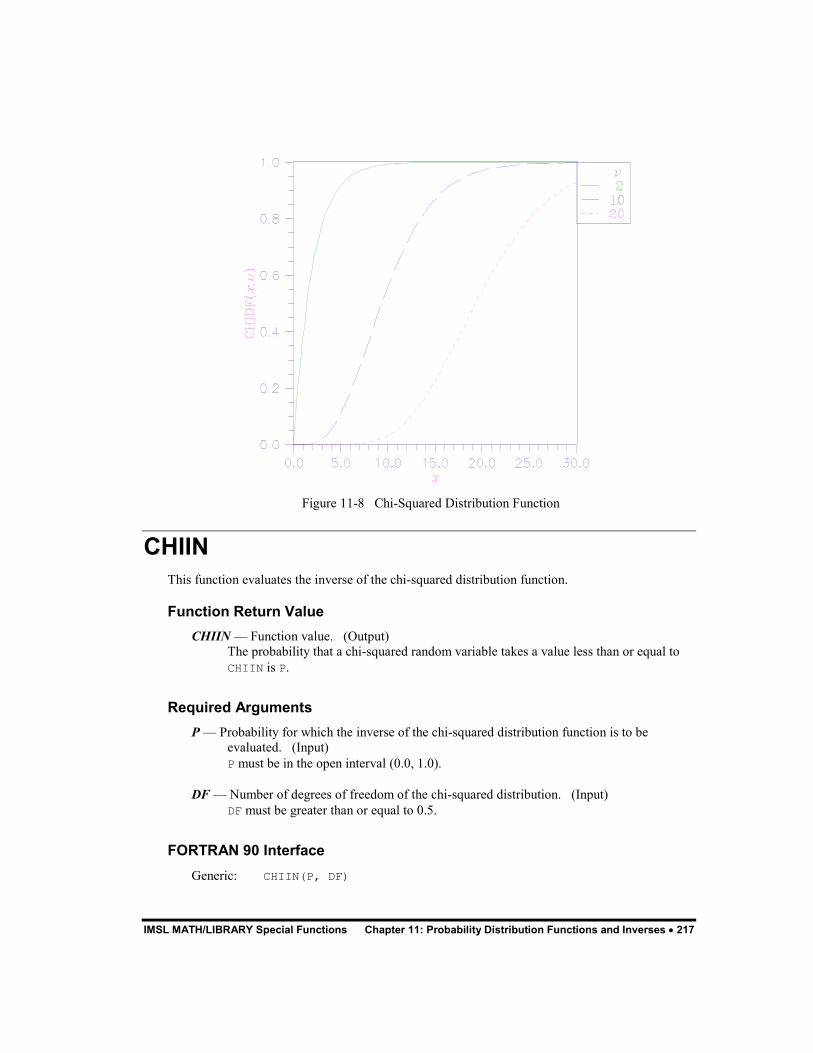
IMSL MATH/LIBRARY Special Functions Chapter 11: Probability Distribution Functions and Inverses � 217
Figure 11-8 Chi-Squared Distribution Function
CHIIN This function evaluates the inverse of the chi-squared distribution function.
Function Return Value CHIIN — Function value. (Output)
The probability that a chi-squared random variable takes a value less than or equal to CHIIN is P.
Required Arguments P — Probability for which the inverse of the chi-squared distribution function is to be
evaluated. (Input) P must be in the open interval (0.0, 1.0).
DF — Number of degrees of freedom of the chi-squared distribution. (Input) DF must be greater than or equal to 0.5.
FORTRAN 90 Interface Generic: CHIIN(P, DF)
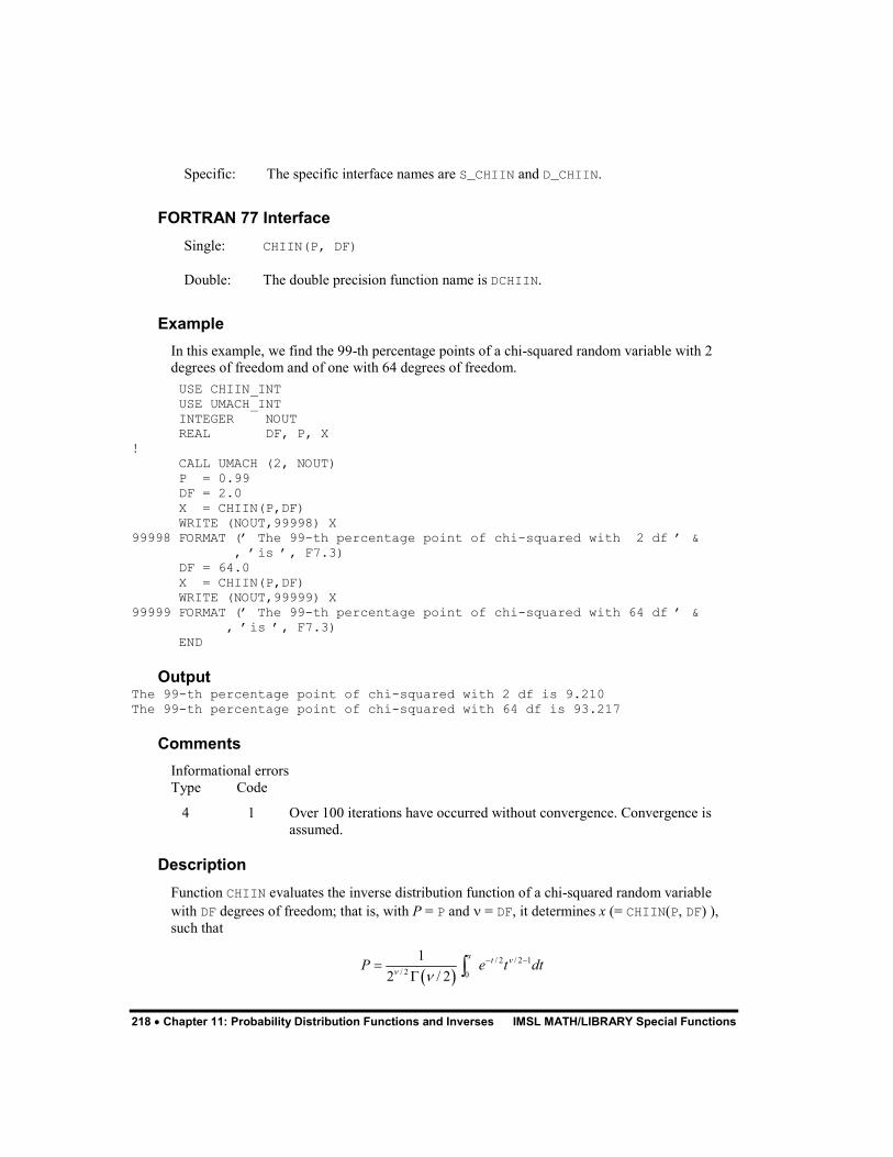
218 � Chapter 11: Probability Distribution Functions and Inverses IMSL MATH/LIBRARY Special Functions
Specific: The specific interface names are S_CHIIN and D_CHIIN.
FORTRAN 77 Interface Single: CHIIN(P, DF)
Double: The double precision function name is DCHIIN.
Example In this example, we find the 99-th percentage points of a chi-squared random variable with 2 degrees of freedom and of one with 64 degrees of freedom.
USE CHIIN_INT USE UMACH_INT INTEGER NOUT REAL DF, P, X ! CALL UMACH (2, NOUT) P = 0.99 DF = 2.0 X = CHIIN(P,DF) WRITE (NOUT,99998) X 99998 FORMAT (’ The 99-th percentage point of chi-squared with 2 df ’ & , ’is ’, F7.3) DF = 64.0 X = CHIIN(P,DF) WRITE (NOUT,99999) X 99999 FORMAT (’ The 99-th percentage point of chi-squared with 64 df ’ & , ’is ’, F7.3) END
Output The 99-th percentage point of chi-squared with 2 df is 9.210 The 99-th percentage point of chi-squared with 64 df is 93.217
Comments Informational errors Type Code
4 1 Over 100 iterations have occurred without convergence. Convergence is assumed.
Description Function CHIIN evaluates the inverse distribution function of a chi-squared random variable with DF degrees of freedom; that is, with P = P and = DF, it determines x (= CHIIN(P, DF) ), such that
� �/ 2 / 2 1
/ 2 0
12 / 2
x t vP e t dt�
�
� ��� �
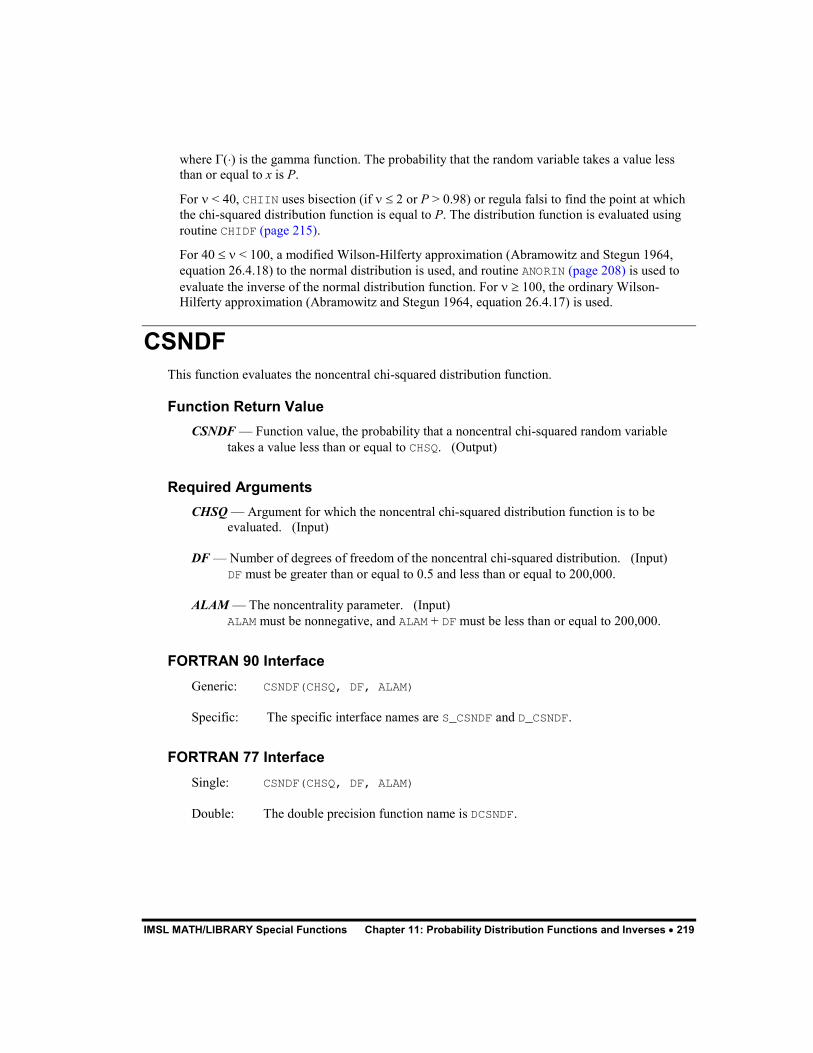
IMSL MATH/LIBRARY Special Functions Chapter 11: Probability Distribution Functions and Inverses � 219
where (�) is the gamma function. The probability that the random variable takes a value less than or equal to x is P.
For < 40, CHIIN uses bisection (if � 2 or P > 0.98) or regula falsi to find the point at which the chi-squared distribution function is equal to P. The distribution function is evaluated using routine CHIDF (page 215).
For 40 � < 100, a modified Wilson-Hilferty approximation (Abramowitz and Stegun 1964, equation 26.4.18) to the normal distribution is used, and routine ANORIN (page 208) is used to evaluate the inverse of the normal distribution function. For � 100, the ordinary Wilson-Hilferty approximation (Abramowitz and Stegun 1964, equation 26.4.17) is used.
CSNDF This function evaluates the noncentral chi-squared distribution function.
Function Return Value CSNDF — Function value, the probability that a noncentral chi-squared random variable
takes a value less than or equal to CHSQ. (Output)
Required Arguments CHSQ — Argument for which the noncentral chi-squared distribution function is to be
evaluated. (Input)
DF — Number of degrees of freedom of the noncentral chi-squared distribution. (Input) DF must be greater than or equal to 0.5 and less than or equal to 200,000.
ALAM — The noncentrality parameter. (Input) ALAM must be nonnegative, and ALAM + DF must be less than or equal to 200,000.
FORTRAN 90 Interface Generic: CSNDF(CHSQ, DF, ALAM)
Specific: The specific interface names are S_CSNDF and D_CSNDF.
FORTRAN 77 Interface Single: CSNDF(CHSQ, DF, ALAM)
Double: The double precision function name is DCSNDF.
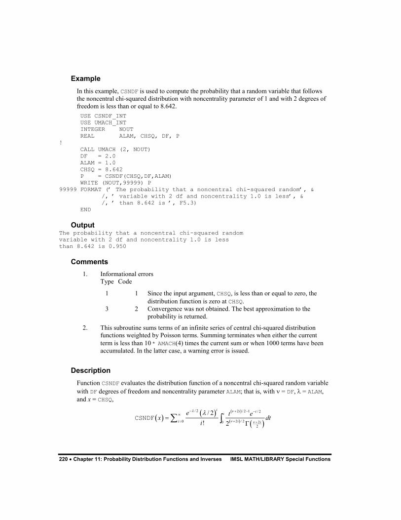
220 � Chapter 11: Probability Distribution Functions and Inverses IMSL MATH/LIBRARY Special Functions
Example In this example, CSNDF is used to compute the probability that a random variable that follows the noncentral chi-squared distribution with noncentrality parameter of 1 and with 2 degrees of freedom is less than or equal to 8.642.
USE CSNDF_INT USE UMACH_INT INTEGER NOUT REAL ALAM, CHSQ, DF, P ! CALL UMACH (2, NOUT) DF = 2.0 ALAM = 1.0 CHSQ = 8.642 P = CSNDF(CHSQ,DF,ALAM) WRITE (NOUT,99999) P 99999 FORMAT (’ The probability that a noncentral chi-squared random’, & /, ’ variable with 2 df and noncentrality 1.0 is less’, & /, ’ than 8.642 is ’, F5.3) END
Output The probability that a noncentral chi-squared random variable with 2 df and noncentrality 1.0 is less than 8.642 is 0.950
Comments 1. Informational errors
Type Code
1 1 Since the input argument, CHSQ, is less than or equal to zero, the distribution function is zero at CHSQ.
3 2 Convergence was not obtained. The best approximation to the probability is returned.
2. This subroutine sums terms of an infinite series of central chi-squared distribution functions weighted by Poisson terms. Summing terminates when either the current term is less than 10 * AMACH(4) times the current sum or when 1000 terms have been accumulated. In the latter case, a warning error is issued.
Description Function CSNDF evaluates the distribution function of a noncentral chi-squared random variable with DF degrees of freedom and noncentrality parameter ALAM; that is, with = DF, � = ALAM, and x = CHSQ,
� �� � � �
� � � �
/ 2 2 / 2 1 / 2
2 / 20 202
/ 2! 2
i i tx
ii i
e t ex dti
� �
� �
�� � � �
�
�� �
�
�� �CSNDF

IMSL MATH/LIBRARY Special Functions Chapter 11: Probability Distribution Functions and Inverses � 221
where (�) is the gamma function. This is a series of central chi-squared distribution functions with Poisson weights. The value of the distribution function at the point x is the probability that the random variable takes a value less than or equal to x.
The noncentral chi-squared random variable can be defined by the distribution function above, or alternatively and equivalently, as the sum of squares of independent normal random variables. If Yi have independent normal distributions with means �i and variances equal to one and
21
nii
X Y�
��
then X has a noncentral chi-squared distribution with n degrees of freedom and noncentrality parameter equal to
21
nii
��
�
With a noncentrality parameter of zero, the noncentral chi-squared distribution is the same as the chi-squared distribution.
Function CSNDF determines the point at which the Poisson weight is greatest, and then sums forward and backward from that point, terminating when the additional terms are sufficiently small or when a maximum of 1000 terms have been accumulated. The recurrence relation 26.4.8 of Abramowitz and Stegun (1964) is used to speed the evaluation of the central chi-squared distribution functions.
Figure 11-9 Noncentral Chi-squared Distribution Function

222 � Chapter 11: Probability Distribution Functions and Inverses IMSL MATH/LIBRARY Special Functions
FDF This function evaluates the F distribution function.
Function Return Value FDF — Function value, the probability that an F random variable takes a value less than or
equal to the input F. (Output)
Required Arguments F — Argument for which the F distribution function is to be evaluated. (Input)
DFN — Numerator degrees of freedom. (Input) DFN must be positive.
DFD — Denominator degrees of freedom. (Input) DFD must be positive.
FORTRAN 90 Interface Generic: FDF(F, DFN, DFD)
Specific: The specific interface names are S_FDF and D_FDF.
FORTRAN 77 Interface Single: FDF(F, DFN, DFD)
Double: The double precision function name is DFDF.
Example In this example, we find the probability that an F random variable with one numerator and one denominator degree of freedom is greater than 648.
USE FDF_INT USE UMACH_INT INTEGER NOUT REAL DFD, DFN, F, P ! CALL UMACH (2, NOUT) F = 648.0 DFN = 1.0 DFD = 1.0 P = 1.0 - FDF(F,DFN,DFD) WRITE (NOUT,99999) P 99999 FORMAT (’ The probability that an F(1,1) variate is greater ’, & ’than 648 is ’, F6.4) END
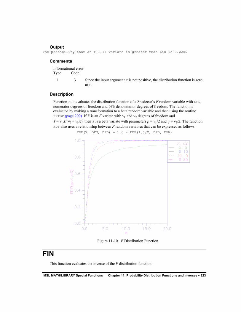
IMSL MATH/LIBRARY Special Functions Chapter 11: Probability Distribution Functions and Inverses � 223
Output The probability that an F(1,1) variate is greater than 648 is 0.0250
Comments Informational error Type Code
1 3 Since the input argument F is not positive, the distribution function is zero at F.
Description Function FDF evaluates the distribution function of a Snedecor’s F random variable with DFN numerator degrees of freedom and DFD denominator degrees of freedom. The function is evaluated by making a transformation to a beta random variable and then using the routine BETDF (page 209). If X is an F variate with � and � degrees of freedom and Y = �X/( � + �X), then Y is a beta variate with parameters p = �/2 and q = �/2. The function FDF also uses a relationship between F random variables that can be expressed as follows:
FDF(X, DFN, DFD) = 1.0 - FDF(1.0/X, DFD, DFN)
Figure 11-10 F Distribution Function
FIN This function evaluates the inverse of the F distribution function.

224 � Chapter 11: Probability Distribution Functions and Inverses IMSL MATH/LIBRARY Special Functions
Function Return Value FIN — Function value. (Output)
The probability that an F random variable takes a value less than or equal to FIN is P.
Required Arguments P — Probability for which the inverse of the F distribution function is to be evaluated.
(Input) P must be in the open interval (0.0, 1.0).
DFN — Numerator degrees of freedom. (Input) DFN must be positive.
DFD — Denominator degrees of freedom. (Input) DFD must be positive.
FORTRAN 90 Interface Generic: FIN(P, DFN, DFD)
Specific: The specific interface names are S_FIN and D_FIN.
FORTRAN 77 Interface Single: FIN(P, DFN, DFD)
Double: The double precision function name is DFIN.
Example In this example, we find the 99-th percentage point for an F random variable with 1 and 7 degrees of freedom.
USE FIN_INT USE UMACH_INT INTEGER NOUT REAL DFD, DFN, F, P ! CALL UMACH (2, NOUT) P = 0.99 DFN = 1.0 DFD = 7.0 F = FIN(P,DFN,DFD) WRITE (NOUT,99999) F 99999 FORMAT (’ The F(1,7) 0.01 critical value is ’, F6.3) END
IMSL MATH/LIBRARY Special Functions Chapter 11: Probability Distribution Functions and Inverses � 225
Output The F(1,7) 0.01 critical value is 12.246
Comments Informational error Type Code
4 4 FIN is set to machine infinity since overflow would occur upon modifying the inverse value for the F distribution with the result obtained from the inverse BETA distribution.
Description Function FIN evaluates the inverse distribution function of a Snedecor’s F random variable with DFN numerator degrees of freedom and DFD denominator degrees of freedom. The function is evaluated by making a transformation to a beta random variable and then using the routine BETIN (page 212). If X is an F variate with 1 and 2 degrees of freedom and Y = �X/( � + �X), then Y is a beta variate with parameters p = �/2 and q = �/2. If P � 0.5, FIN uses this relationship directly; otherwise, it also uses a relationship between F random variables that can be expressed as follows, using routine FDF (page 222), which is the F cumulative distribution function:
FDF(F, DFN, DFD) = 1.0 - FDF(1.0/F, DFD, DFN)
GAMDF This function evaluates the gamma distribution function.
Function Return Value GAMDF — Function value, the probability that a gamma random variable takes a value less
than or equal to X. (Output)
Required Arguments X — Argument for which the gamma distribution function is to be evaluated. (Input)
A — The shape parameter of the gamma distribution. (Input) This parameter must be positive.
FORTRAN 90 Interface Generic: GAMDF(X, A)
Specific: The specific interface names are S_GAMDF and D_GAMDF.
226 � Chapter 11: Probability Distribution Functions and Inverses IMSL MATH/LIBRARY Special Functions
FORTRAN 77 Interface Single: GAMDF(X, A)
Double: The double precision function name is DGAMDF.
Example Suppose X is a gamma random variable with a shape parameter of 4. (In this case, it has an Erlang distribution since the shape parameter is an integer.) In this example, we find the probability that X is less than 0.5 and the probability that X is between 0.5 and 1.0.
USE GAMDF_INT USE UMACH_INT INTEGER NOUT REAL A, P, X ! CALL UMACH (2, NOUT) A = 4.0 X = 0.5 P = GAMDF(X,A) WRITE (NOUT,99998) P 99998 FORMAT (’ The probability that X is less than 0.5 is ’, F6.4) X = 1.0 P = GAMDF(X,A) - P WRITE (NOUT,99999) P 99999 FORMAT (’ The probability that X is between 0.5 and 1.0 is ’, & F6.4) END
Output The probability that X is less than 0.5 is 0.0018 The probability that X is between 0.5 and 1.0 is 0.0172
Comments Informational error Type Code
1 2 Since the input argument X is less than zero, the distribution function is set to zero.
Description Function GAMDF evaluates the distribution function, F , of a gamma random variable with shape parameter a; that is,
� �� �
1
0
1 x t aF x e t dta
� �
��
�
where (�) is the gamma function. (The gamma function is the integral from 0 to � of the same integrand as above). The value of the distribution function at the point x is the probability that the random variable takes a value less than or equal to x.
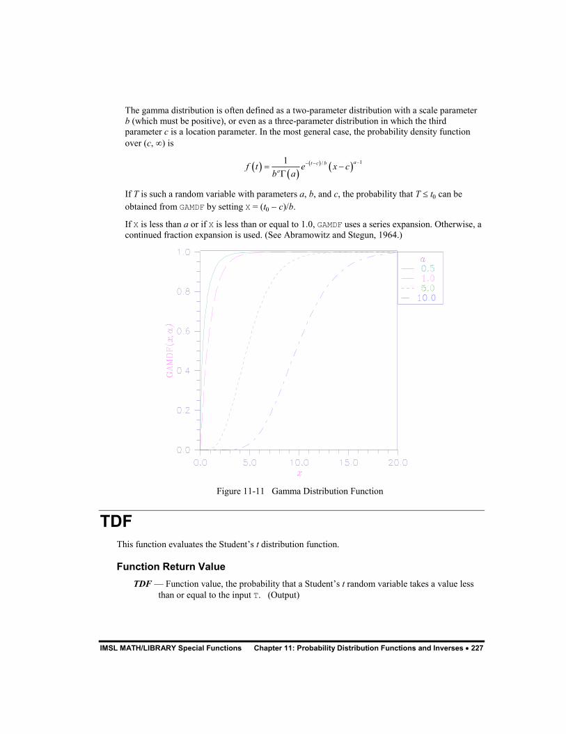
IMSL MATH/LIBRARY Special Functions Chapter 11: Probability Distribution Functions and Inverses � 227
The gamma distribution is often defined as a two-parameter distribution with a scale parameter b (which must be positive), or even as a three-parameter distribution in which the third parameter c is a location parameter. In the most general case, the probability density function over (c, �) is
� �� �
� � � �1/1 at c b
af t e x cb a
�� �
� ��
If T is such a random variable with parameters a, b, and c, the probability that T � t� can be obtained from GAMDF by setting X = (t� � c)/b.
If X is less than a or if X is less than or equal to 1.0, GAMDF uses a series expansion. Otherwise, a continued fraction expansion is used. (See Abramowitz and Stegun, 1964.)
Figure 11-11 Gamma Distribution Function
TDF This function evaluates the Student’s t distribution function.
Function Return Value TDF — Function value, the probability that a Student’s t random variable takes a value less
than or equal to the input T. (Output)
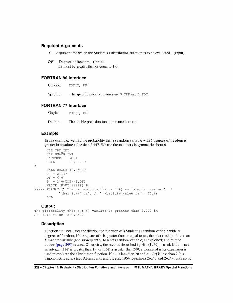
228 � Chapter 11: Probability Distribution Functions and Inverses IMSL MATH/LIBRARY Special Functions
Required Arguments T — Argument for which the Student’s t distribution function is to be evaluated. (Input)
DF — Degrees of freedom. (Input) DF must be greater than or equal to 1.0.
FORTRAN 90 Interface Generic: TDF(T, DF)
Specific: The specific interface names are S_TDF and D_TDF.
FORTRAN 77 Interface Single: TDF(T, DF)
Double: The double precision function name is DTDF.
Example In this example, we find the probability that a t random variable with 6 degrees of freedom is greater in absolute value than 2.447. We use the fact that t is symmetric about 0.
USE TDF_INT USE UMACH_INT INTEGER NOUT REAL DF, P, T ! CALL UMACH (2, NOUT) T = 2.447 DF = 6.0 P = 2.0*TDF(-T,DF) WRITE (NOUT,99999) P 99999 FORMAT (’ The probability that a t(6) variate is greater ’, & ’than 2.447 in’, /, ’ absolute value is ’, F6.4) END
Output The probability that a t(6) variate is greater than 2.447 in absolute value is 0.0500
Description Function TDF evaluates the distribution function of a Student’s t random variable with DF degrees of freedom. If the square of T is greater than or equal to DF, the relationship of a t to an F random variable (and subsequently, to a beta random variable) is exploited; and routine BETDF (page 209) is used. Otherwise, the method described by Hill (1970) is used. If DF is not an integer, if DF is greater than 19, or if DF is greater than 200, a Cornish-Fisher expansion is used to evaluate the distribution function. If DF is less than 20 and ABS(T) is less than 2.0, a trigonometric series (see Abramowitz and Stegun, 1964, equations 26.7.3 and 26.7.4, with some
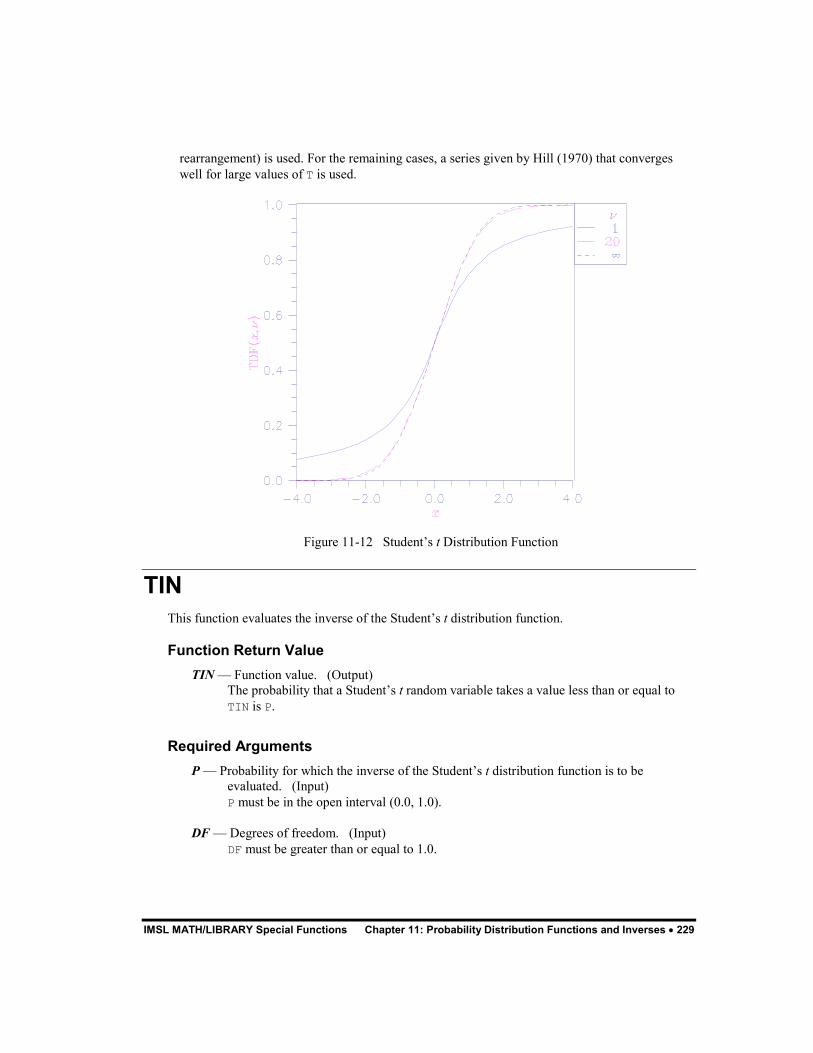
IMSL MATH/LIBRARY Special Functions Chapter 11: Probability Distribution Functions and Inverses � 229
rearrangement) is used. For the remaining cases, a series given by Hill (1970) that converges well for large values of T is used.
Figure 11-12 Student’s t Distribution Function
TIN This function evaluates the inverse of the Student’s t distribution function.
Function Return Value TIN — Function value. (Output)
The probability that a Student’s t random variable takes a value less than or equal to TIN is P.
Required Arguments P — Probability for which the inverse of the Student’s t distribution function is to be
evaluated. (Input) P must be in the open interval (0.0, 1.0).
DF — Degrees of freedom. (Input) DF must be greater than or equal to 1.0.

230 � Chapter 11: Probability Distribution Functions and Inverses IMSL MATH/LIBRARY Special Functions
FORTRAN 90 Interface Generic: TIN(P, DF)
Specific: The specific interface names are S_TIN and D_TIN.
FORTRAN 77 Interface Single: TIN(P, DF)
Double: The double precision function name is DTIN.
Example In this example, we find the 0.05 critical value for a two-sided t test with 6 degrees of freedom.
USE TIN_INT USE UMACH_INT INTEGER NOUT REAL DF, P, T ! CALL UMACH (2, NOUT) P = 0.975 DF = 6.0 T = TIN(P,DF) WRITE (NOUT,99999) T 99999 FORMAT (’ The two-sided t(6) 0.05 critical value is ’, F6.3) END
Output The two-sided t(6) 0.05 critical value is 2.447
Comments Informational error Type Code
4 3 TIN is set to machine infinity since overflow would occur upon modifying the inverse value for the F distribution with the result obtained from the inverse � distribution.
Description Function TIN evaluates the inverse distribution function of a Student’s t random variable with DF degrees of freedom. Let = DF. If equals 1 or 2, the inverse can be obtained in closed form; if is between 1 and 2, the relationship of a t to a beta random variable is exploited and routine BETIN (page 212) is used to evaluate the inverse; otherwise the algorithm of Hill (1970) is used. For small values of greater than 2, Hill’s algorithm inverts an integrated expansion in 1/(1 + t�/ ) of the t density. For larger values, an asymptotic inverse Cornish-Fisher type expansion about normal deviates is used.
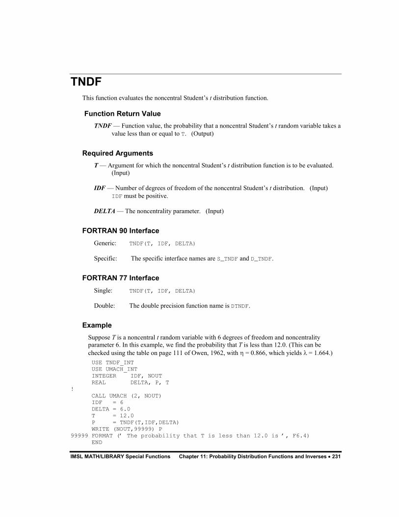
IMSL MATH/LIBRARY Special Functions Chapter 11: Probability Distribution Functions and Inverses � 231
TNDF This function evaluates the noncentral Student’s t distribution function.
Function Return Value TNDF — Function value, the probability that a noncentral Student’s t random variable takes a
value less than or equal to T. (Output)
Required Arguments T — Argument for which the noncentral Student’s t distribution function is to be evaluated.
(Input)
IDF — Number of degrees of freedom of the noncentral Student’s t distribution. (Input) IDF must be positive.
DELTA — The noncentrality parameter. (Input)
FORTRAN 90 Interface Generic: TNDF(T, IDF, DELTA)
Specific: The specific interface names are S_TNDF and D_TNDF.
FORTRAN 77 Interface Single: TNDF(T, IDF, DELTA)
Double: The double precision function name is DTNDF.
Example Suppose T is a noncentral t random variable with 6 degrees of freedom and noncentrality parameter 6. In this example, we find the probability that T is less than 12.0. (This can be checked using the table on page 111 of Owen, 1962, with � = 0.866, which yields � = 1.664.)
USE TNDF_INT USE UMACH_INT INTEGER IDF, NOUT REAL DELTA, P, T ! CALL UMACH (2, NOUT) IDF = 6 DELTA = 6.0 T = 12.0 P = TNDF(T,IDF,DELTA) WRITE (NOUT,99999) P 99999 FORMAT (’ The probability that T is less than 12.0 is ’, F6.4) END

232 � Chapter 11: Probability Distribution Functions and Inverses IMSL MATH/LIBRARY Special Functions
Output The probability that T is less than 12.0 is 0.9501
Description Function TNDF evaluates the distribution function F of a noncentral t random variable with IDF degrees of freedom and noncentrality parameter DELTA; that is, with = IDF, � = DELTA , and t� = T,
� �� �� �
� �
� �� �
2
0/ 2 / 2
0 1 / 22
/ 22
20
/ 2
21 / 2!
t
ii
i
eF tx
xi dxi x
� �
�
�
� � �
��
�
�
���
�
�
�� �
� �� �� � � � �� �
�� �
�
�
where (�) is the gamma function. The value of the distribution function at the point t� is the probability that the random variable takes a value less than or equal to t�.
The noncentral t random variable can be defined by the distribution function above, or alternatively and equivalently, as the ratio of a normal random variable and an independent chi-squared random variable. If w has a normal distribution with mean � and variance equal to one, u has an independent chi-squared distribution with degrees of freedom, and
/wu �
then x has a noncentral t distribution with degrees of freedom and noncentrality parameter �.
The distribution function of the noncentral t can also be expressed as a double integral involving a normal density function (see, for example, Owen, 1962, page 108). The function TNDF uses the method of Owen (1962, 1965), which uses repeated integration by parts on that alternate expression for the distribution function.
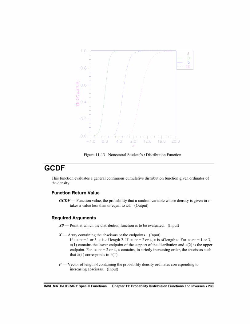
IMSL MATH/LIBRARY Special Functions Chapter 11: Probability Distribution Functions and Inverses � 233
Figure 11-13 Noncentral Student’s t Distribution Function
GCDF This function evaluates a general continuous cumulative distribution function given ordinates of the density.
Function Return Value GCDF — Function value, the probability that a random variable whose density is given in F
takes a value less than or equal to X0. (Output)
Required Arguments X0 — Point at which the distribution function is to be evaluated. (Input)
X — Array containing the abscissas or the endpoints. (Input) If IOPT = 1 or 3, X is of length 2. If IOPT = 2 or 4, X is of length M. For IOPT = 1 or 3, X(1) contains the lower endpoint of the support of the distribution and X(2) is the upper endpoint. For IOPT = 2 or 4, X contains, in strictly increasing order, the abscissas such that X(I) corresponds to F(I).
F — Vector of length M containing the probability density ordinates corresponding to increasing abscissas. (Input)
234 � Chapter 11: Probability Distribution Functions and Inverses IMSL MATH/LIBRARY Special Functions
If IOPT = 1 or 3; for I = 1, 2, �, M, F(I) corresponds to X(1) + (I � 1) * (X(2) � X(1))/(M � 1); otherwise, F and X correspond one for one.
Optional Arguments IOPT — Indicator of the method of interpolation. (Input)
Default: IOPT = 1.
IOPT Interpolation Method 1 Linear interpolation with equally spaced abscissas. 2 Linear interpolation with possibly unequally spaced abscissas. 3 A cubic spline is fitted to equally spaced abscissas. 4 A cubic spline is fitted to possibly unequally spaced abscissas.
M — Number of ordinates of the density supplied. (Input) M must be greater than 1 for linear interpolation (IOPT = 1 or 2) and greater than 3 if a curve is fitted through the ordinates (IOPT = 3 or 4). Default: M = size (F,1).
FORTRAN 90 Interface Generic: GCDF (X0, X, F [,…])
Specific: The specific interface names are S_GCDF and D_GCDF.
FORTRAN 77 Interface Single: GCDF(X0, IOPT, M, X, F)
Double: The double precision functin name is DGCDF.
Example In this example, we evaluate the beta distribution function at the point 0.6. The probability density function of a beta random variable with parameters p and q is
� �� �
� � � �� �
11 1 for 0 1qpp qf x x x x
p q�
�
� �� � � �� �
where (�) is the gamma function. The density is equal to 0 outside the interval [0, 1]. We compute a constant multiple (we can ignore the constant gamma functions) of the density at 300 equally spaced points and input this information in X and F. Knowing that the probability density of this distribution is very peaked in the vicinity of 0.5, we could perhaps get a better fit by using unequally spaced abscissas, but we will keep it simple. Note that this is the same example as one used in the description of routine BETDF (page 209). The result from BETDF would be expected to be more accurate than that from GCDF since BETDF is designed specifically for this distribution.
IMSL MATH/LIBRARY Special Functions Chapter 11: Probability Distribution Functions and Inverses � 235
USE GCDF_INT USE UMACH_INT INTEGER M PARAMETER (M=300) ! INTEGER I, IOPT, NOUT REAL F(M), H, P, PIN1, QIN1, X(2), X0, XI ! CALL UMACH (2, NOUT) X0 = 0.6 IOPT = 3 ! Initializations for a beta(12,12) ! distribution. PIN1 = 11.0 QIN1 = 11.0 XI = 0.0 H = 1.0/(M-1.0) X(1) = XI F(1) = 0.0 XI = XI + H ! Compute ordinates of the probability ! density function. DO 10 I=2, M - 1 F(I) = XI**PIN1*(1.0-XI)**QIN1 XI = XI + H 10 CONTINUE X(2) = 1.0 F(M) = 0.0 P = GCDF(X0,X,F, IOPT=IOPT) WRITE (NOUT,99999) P 99999 FORMAT (’ The probability that X is less than 0.6 is ’, F6.4) END
Output The probability that X is less than 0.6 is 0.8364
Comments Workspace may be explicitly provided, if desired, by the use of G4DF/DG4DF. The reference is:
G4DF(P, IOPT, M, X, F, WK, IWK)
The arguments in addition to those of GCDF are:
WK — Work vector of length 5 * M if IOPT = 3, and of length 4 * M if IOPT = 4.
IWK — Work vector of length M.
Description Function GCDF evaluates a continuous distribution function, given ordinates of the probability density function. It requires that the range of the distribution be specified in X. For distributions
236 � Chapter 11: Probability Distribution Functions and Inverses IMSL MATH/LIBRARY Special Functions
with infinite ranges, endpoints must be chosen so that most of the probability content is included. The function GCDF first fits a curve to the points given in X and F with either a piecewise linear interpolant or a C� cubic spline interpolant based on a method by Akima (1970). Function GCDF then determines the area, A, under the curve. (If the distribution were of finite range and if the fit were exact, this area would be 1.0.) Using the same fitted curve, GCDF next determines the area up to the point x� (= X0). The value returned is the area up to x� divided by A. Because of the scaling by A, it is not assumed that the integral of the density defined by X and F is 1.0.
For most distributions, it is likely that better approximations to the distribution function are obtained when IOPT equals 3 or 4, that is, when a cubic spline is used to approximate the function. It is also likely that better approximations can be obtained when the abscissas are chosen more densely over regions where the density and its derivatives (when they exist) are varying greatly.
GCIN Evaluates the inverse of a general continuous cumulative distribution function given ordinates of the density.
Required Arguments P — Probability for which the inverse of the distribution function is to be evaluated. (Input)
P must be in the open interval (0.0, 1.0).
X — Array containing the abscissas or the endpoints. (Input) If IOPT = 1 or 3, X is of length 2. If IOPT = 2 or 4, X is of length M. For IOPT = 1 or 3, X(1) contains the lower endpoint of the support of the distribution and X(2) is the upper endpoint. For IOPT = 2 or 4, X contains, in strictly increasing order, the abscissas such that X(I) corresponds to F(I).
F — Vector of length M containing the probability density ordinates corresponding to increasing abscissas. (Input) If IOPT = 1 or 3, for I = 1, 2, �, M, F(I) corresponds to X(1) + (I � 1) * (X(2) � X(1))/(M � 1); otherwise, F and X correspond one for one.
GCIN — Function value. (Output) The probability that a random variable whose density is given in F takes a value less than or equal to GCIN is P.
Optional Arguments IOPT — Indicator of the method of interpolation. (Input)
Default: IOPT = 1.
IOPT Interpolation Method 1 Linear interpolation with equally spaced abscissas. 2 Linear interpolation with possibly unequally spaced abscissas.

IMSL MATH/LIBRARY Special Functions Chapter 11: Probability Distribution Functions and Inverses � 237
3 A cubic spline is fitted to equally spaced abscissas. 4 A cubic spline is fitted to possibly unequally spaced abscissas.
M — Number of ordinates of the density supplied. (Input) M must be greater than 1 for linear interpolation (IOPT = 1 or 2) and greater than 3 if a curve is fitted through the ordinates (IOPT = 3 or 4). Default: M = size (F,1).
FORTRAN 90 Interface Generic: CALL GCIN (P, X, F [,…])
Specific: The specific interface names are S_GCIN and D_GCIN.
FORTRAN 77 Interface Single: CALL GCIN(P, IOPT, M, X, F)
Double: The double precision function name is DGCIN.
Example In this example, we find the 90-th percentage point for a beta random variable with parameters 12 and 12. The probability density function of a beta random variable with parameters p and q is
� �� �
� � � �� �
11 1 for 0 1qpp qf x x x x
p q�
�
� �� � � �� �
where (�) is the gamma function. The density is equal to 0 outside the interval [0, 1]. With p = q, this is a symmetric distribution. Knowing that the probability density of this distribution is very peaked in the vicinity of 0.5, we could perhaps get a better fit by using unequally spaced abscissas, but we will keep it simple and use 300 equally spaced points. Note that this is the same example that is used in the description of routine BETIN (page 212). The result from BETIN would be expected to be more accurate than that from GCIN since BETIN is designed specifically for this distribution.
USE GCIN_INT USE UMACH_INT USE BETA_INT INTEGER M PARAMETER (M=300) ! INTEGER I, IOPT, NOUT REAL C, F(M), H, P, PIN, PIN1, QIN, QIN1, & X(2), X0, XI ! CALL UMACH (2, NOUT) P = 0.9 IOPT = 3 ! Initializations for a beta(12,12) ! distribution.
238 � Chapter 11: Probability Distribution Functions and Inverses IMSL MATH/LIBRARY Special Functions
PIN = 12.0 QIN = 12.0 PIN1 = PIN - 1.0 QIN1 = QIN - 1.0 C = 1.0/BETA(PIN,QIN) XI = 0.0 H = 1.0/(M-1.0) X(1) = XI F(1) = 0.0 XI = XI + H ! Compute ordinates of the probability ! density function. DO 10 I=2, M - 1 F(I) = C*XI**PIN1*(1.0-XI)**QIN1 XI = XI + H 10 CONTINUE X(2) = 1.0 F(M) = 0.0 X0 = GCIN(P,X,F, IOPT=IOPT) WRITE (NOUT,99999) X0 99999 FORMAT (’ X is less than ’, F6.4, ’ with probability 0.9.’) END
Output X is less than 0.6304 with probability 0.9.
Comments Workspace may be explicitly provided, if desired, by the use of G3IN/DG3IN. The reference is
G3IN(P, IOPT, M, X, F, WK, IWK)
The arguments in addition to those of GCIN are:
WK — Work vector of length 5 * M if IOPT = 3, and of length 4 * M if IOPT = 4.
IWK — Work vector of length M.
Description Function GCIN evaluates the inverse of a continuous distribution function, given ordinates of the probability density function. The range of the distribution must be specified in X. For distributions with infinite ranges, endpoints must be chosen so that most of the probability content is included.
The function GCIN first fits a curve to the points given in X and F with either a piecewise linear interpolant or a C� cubic spline interpolant based on a method by Akima (1970). Function GCIN then determines the area, A, under the curve. (If the distribution were of finite range and if the fit were exact, this area would be 1.0.) It next finds the maximum abscissa up to which the area is less than AP and the minimum abscissa up to which the area is greater than AP. The routine then interpolates for the point corresponding to AP. Because of the scaling by A, it is not assumed that the integral of the density defined by X and F is 1.0.

IMSL MATH/LIBRARY Special Functions Chapter 11: Probability Distribution Functions and Inverses � 239
For most distributions, it is likely that better approximations to the distribution function are obtained when IOPT equals 3 or 4, that is, when a cubic spline is used to approximate the function. It is also likely that better approximations can be obtained when the abscissas are chosen more densely over regions where the density and its derivatives (when they exist) are varying greatly.

240 � Chapter 11: Probability Distribution Functions and Inverses IMSL MATH/LIBRARY Special Functions
IMSL MATH/LIBRARY Special Functions Chapter 12: Mathieu Functions � 241
Chapter 12: Mathieu Functions
Routines Evaluate the eigenvalues for the periodic Mathieu functions........................................MATEE 241 Evaluate even, periodic Mathieu functions ......................... MATCE 244 Evaluate odd, periodic Mathieu functions............................MATSE 248
Usage Notes Mathieu’s equation is
� �2
2 2 cos 2 0d y a q v ydv
� � �
It arises from the solution, by separation of variables, of Laplace’s equation in elliptical coordinates, where a is the separation constant and q is related to the ellipticity of the coordinate system. If we let t = cos v, then Mathieu’s equation can be written as
� � � �2
2 221 2 4 0d y dyt t a q qt y
dtdt� � � � � �
For various physically important problems, the solution y(t) must be periodic. There exist, for particular values of a, periodic solutions to Mathieu’s equation of period k� for any integer k. These particular values of a are called eigenvalues or characteristic values. They are computed using the routine MATEE (page 241).
There exist sequences of both even and odd periodic solutions to Mathieu’s equation. The even solutions are computed by MATCE (page 244). The odd solutions are computed by MATSE (page 246).
MATEE Evaluates the eigenvalues for the periodic Mathieu functions.
Required Arguments Q — Parameter. (Input)
242 � Chapter 12: Mathieu Functions IMSL MATH/LIBRARY Special Functions
ISYM — Symmetry indicator. (Input)
ISYM Meaning 0 Even 1 Odd
IPER — Periodicity indicator. (Input)
ISYM Period 0 pi 1 2 * pi
EVAL — Vector of length N containing the eigenvalues. (Output)
Optional Arguments N — Number of eigenvalues to be computed. (Input)
Default: N = size (EVAL,1)
FORTRAN 90 Interface Generic: CALL MATEE (Q, ISYM, IPER, EVAL [,…])
Specific: The specific interface names are S_MATEE and D_MATEE.
FORTRAN 77 Interface Single: CALL MATEE (Q, N, ISYM, IPER, EVAL)
Double: The double precision function name is DMATEE.
Example In this example, the eigenvalues for q = 5, even symmetry, and � periodicity are computed and printed.
USE UMACH_INT USE MATEE_INT ! Declare variables INTEGER N PARAMETER (N=10) ! INTEGER ISYM, IPER, K, NOUT REAL Q, EVAL(N) ! Compute Q = 5.0 ISYM = 0 IPER = 0 CALL MATEE (Q, ISYM, IPER, EVAL) ! Print the results CALL UMACH (2, NOUT)
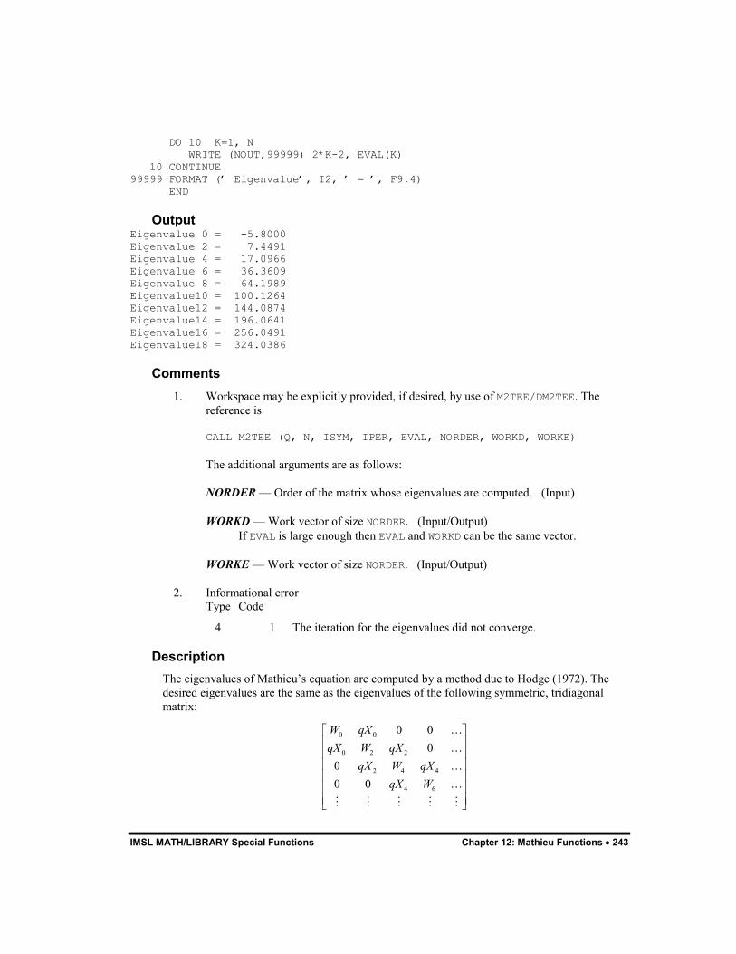
IMSL MATH/LIBRARY Special Functions Chapter 12: Mathieu Functions � 243
DO 10 K=1, N WRITE (NOUT,99999) 2*K-2, EVAL(K) 10 CONTINUE 99999 FORMAT (’ Eigenvalue’, I2, ’ = ’, F9.4) END
Output Eigenvalue 0 = -5.8000 Eigenvalue 2 = 7.4491 Eigenvalue 4 = 17.0966 Eigenvalue 6 = 36.3609 Eigenvalue 8 = 64.1989 Eigenvalue10 = 100.1264 Eigenvalue12 = 144.0874 Eigenvalue14 = 196.0641 Eigenvalue16 = 256.0491 Eigenvalue18 = 324.0386
Comments 1. Workspace may be explicitly provided, if desired, by use of M2TEE/DM2TEE. The
reference is
CALL M2TEE (Q, N, ISYM, IPER, EVAL, NORDER, WORKD, WORKE)
The additional arguments are as follows:
NORDER — Order of the matrix whose eigenvalues are computed. (Input)
WORKD — Work vector of size NORDER. (Input/Output) If EVAL is large enough then EVAL and WORKD can be the same vector.
WORKE — Work vector of size NORDER. (Input/Output)
2. Informational error Type Code
4 1 The iteration for the eigenvalues did not converge.
Description The eigenvalues of Mathieu’s equation are computed by a method due to Hodge (1972). The desired eigenvalues are the same as the eigenvalues of the following symmetric, tridiagonal matrix:
0 0
0 2 2
2 4 4
4 6
0 00
00 0
W qXqX W qX
qX W qXqX W
� �� �� �� �� �� �� �� �
�
�
�
�
� � � � �
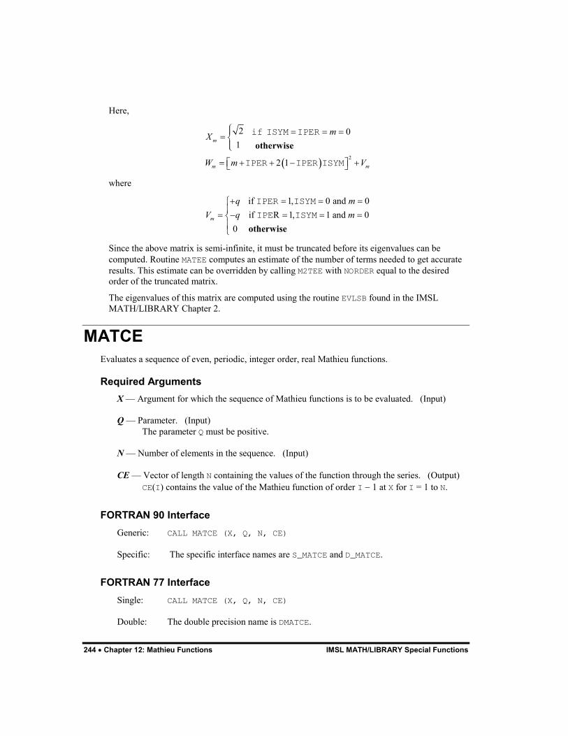
244 � Chapter 12: Mathieu Functions IMSL MATH/LIBRARY Special Functions
Here,
� �2
2 01
2 1
m
m m
mX
W m V
�� � � �� ���
� � � � �� �
otherwiseif ISYM IPER
IPER IPER ISYM
where
if 1, 0 and 0if R 1, 1 and 0
0 m
q mV q m
� � � ���
� � � � ���� otherwise
IPER ISYM
IPE ISYM
Since the above matrix is semi-infinite, it must be truncated before its eigenvalues can be computed. Routine MATEE computes an estimate of the number of terms needed to get accurate results. This estimate can be overridden by calling M2TEE with NORDER equal to the desired order of the truncated matrix.
The eigenvalues of this matrix are computed using the routine EVLSB found in the IMSL MATH/LIBRARY Chapter 2.
MATCE Evaluates a sequence of even, periodic, integer order, real Mathieu functions.
Required Arguments X — Argument for which the sequence of Mathieu functions is to be evaluated. (Input)
Q — Parameter. (Input) The parameter Q must be positive.
N — Number of elements in the sequence. (Input)
CE — Vector of length N containing the values of the function through the series. (Output) CE(I) contains the value of the Mathieu function of order I � 1 at X for I = 1 to N.
FORTRAN 90 Interface Generic: CALL MATCE (X, Q, N, CE)
Specific: The specific interface names are S_MATCE and D_MATCE.
FORTRAN 77 Interface Single: CALL MATCE (X, Q, N, CE)
Double: The double precision name is DMATCE.
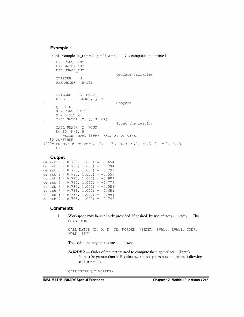
IMSL MATH/LIBRARY Special Functions Chapter 12: Mathieu Functions � 245
Example 1 In this example, cen(x = �/4, q = 1), n = 0, �, 9 is computed and printed.
USE CONST_INT USE MATCE_INT USE UMACH_INT ! Declare variables INTEGER N PARAMETER (N=10) ! INTEGER K, NOUT REAL CE(N), Q, X ! Compute Q = 1.0 X = CONST(’PI’) X = 0.25* X CALL MATCE (X, Q, N, CE) ! Print the results CALL UMACH (2, NOUT) DO 10 K=1, N WRITE (NOUT,99999) K-1, X, Q, CE(K) 10 CONTINUE 99999 FORMAT (’ ce sub’, I2, ’ (’, F6.3, ’,’, F6.3, ’) = ’, F6.3) END
Output ce sub 0 ( 0.785, 1.000) = 0.654 ce sub 1 ( 0.785, 1.000) = 0.794 ce sub 2 ( 0.785, 1.000) = 0.299 ce sub 3 ( 0.785, 1.000) = -0.555 ce sub 4 ( 0.785, 1.000) = -0.989 ce sub 5 ( 0.785, 1.000) = -0.776 ce sub 6 ( 0.785, 1.000) = -0.086 ce sub 7 ( 0.785, 1.000) = 0.654 ce sub 8 ( 0.785, 1.000) = 0.998 ce sub 9 ( 0.785, 1.000) = 0.746
Comments 1. Workspace may be explicitly provided, if desired, by use of M2TCE/DM2TCE. The
reference is
CALL M2TCE (X, Q, N, CE, NORDER, NEEDEV, EVAL0, EVAL1, COEF, WORK, BSJ)
The additional arguments are as follows:
NORDER — Order of the matrix used to compute the eigenvalues. (Input) It must be greater than N. Routine MATSE computes NORDER by the following call to M3TEE.
CALL M3TEE(Q, N, NORDER)
246 � Chapter 12: Mathieu Functions IMSL MATH/LIBRARY Special Functions
NEEDEV — Logical variable, if .TRUE., the eigenvalues must be computed. (Input)
EVAL0 — Real work vector of length NORDER containing the eigenvalues computed by MATEE with ISYM = 0 and IPER = 0. (Input/Output) If NEEDEV is .TRUE., then EVAL0 is computed by M2TCE; otherwise, it must be set as an input value.
EVAL1 — Real work vector of length NORDER containing the eigenvalues computed by MATEE with ISYM = 0 and IPER = 1. (Input/Output) If NEEDEV is .TRUE., then EVAL1 is computed by M2TCE; otherwise, it must be set as an input value.
COEF — Real work vector of length NORDER + 4.
WORK — Real work vector of length NORDER + 4.
BSJ — Real work vector of length 2 * NORDER � 2.
2. Informational error Type Code
4 1 The iteration for the eigenvalues did not converge.
Description The eigenvalues of Mathieu’s equation are computed using MATEE (page 241). The function values are then computed using a sum of Bessel functions, see Gradshteyn and Ryzhik (1965), equation 8.661.
Additional Examples
Example 2 In this example, we compute cen(x, q) for various values of n and x and a fixed value of q. To avoid having to recompute the eigenvalues, which depend on q but not on x, we compute the eigenvalues once and pass in their value to M2TCE. The eigenvalues are computed using MATEE (page 241). The routine M3TEE is used to compute NORDER based on Q and N. The arrays BSJ, COEF and WORK are used as temporary storage in M2TCE.
USE IMSL_LIBRARIES ! Declare variables INTEGER MAXORD, N, NX PARAMETER (MAXORD=100, N=4, NX=5) ! INTEGER ISYM, K, NORDER, NOUT REAL BSJ(2*MAXORD-2), CE(N), COEF(MAXORD+4) REAL EVAL0(MAXORD), EVAL1(MAXORD), PI, Q, WORK(MAXORD+4), X ! Compute NORDER Q = 1.0 CALL M3TEE (Q, N, NORDER)
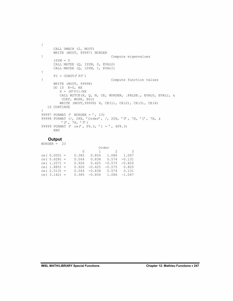
IMSL MATH/LIBRARY Special Functions Chapter 12: Mathieu Functions � 247
! CALL UMACH (2, NOUT) WRITE (NOUT, 99997) NORDER ! Compute eigenvalues ISYM = 0 CALL MATEE (Q, ISYM, 0, EVAL0) CALL MATEE (Q, ISYM, 1, EVAL1) ! PI = CONST(’PI’) ! Compute function values WRITE (NOUT, 99998) DO 10 K=0, NX X = (K*PI)/NX CALL M2TCE(X, Q, N, CE, NORDER, .FALSE., EVAL0, EVAL1, & COEF, WORK, BSJ) WRITE (NOUT,99999) X, CE(1), CE(2), CE(3), CE(4) 10 CONTINUE ! 99997 FORMAT (’ NORDER = ’, I3) 99998 FORMAT (/, 28X, ’Order’, /, 20X, ’0’, 7X, ’1’, 7X, & ’2’, 7X, ’3’) 99999 FORMAT (’ ce(’, F6.3, ’) = ’, 4F8.3) END
Output NORDER = 23 Order 0 1 2 3 ce( 0.000) = 0.385 0.856 1.086 1.067 ce( 0.628) = 0.564 0.838 0.574 -0.131 ce( 1.257) = 0.926 0.425 -0.575 -0.820 ce( 1.885) = 0.926 -0.425 -0.575 0.820 ce( 2.513) = 0.564 -0.838 0.574 0.131 ce( 3.142) = 0.385 -0.856 1.086 -1.067
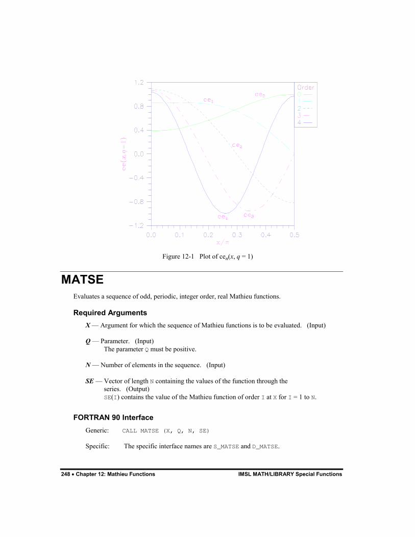
248 � Chapter 12: Mathieu Functions IMSL MATH/LIBRARY Special Functions
Figure 12-1 Plot of cen(x, q = 1)
MATSE Evaluates a sequence of odd, periodic, integer order, real Mathieu functions.
Required Arguments X — Argument for which the sequence of Mathieu functions is to be evaluated. (Input)
Q — Parameter. (Input) The parameter Q must be positive.
N — Number of elements in the sequence. (Input)
SE — Vector of length N containing the values of the function through the series. (Output) SE(I) contains the value of the Mathieu function of order I at X for I = 1 to N.
FORTRAN 90 Interface Generic: CALL MATSE (X, Q, N, SE)
Specific: The specific interface names are S_MATSE and D_MATSE.
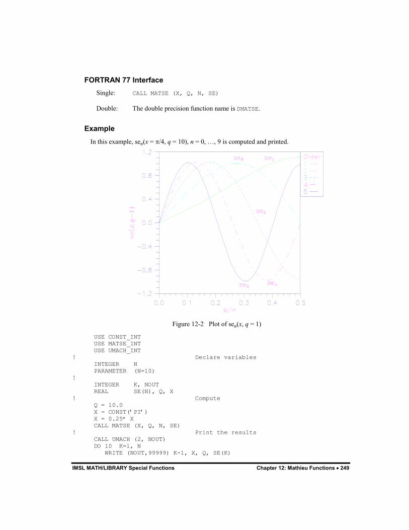
IMSL MATH/LIBRARY Special Functions Chapter 12: Mathieu Functions � 249
FORTRAN 77 Interface Single: CALL MATSE (X, Q, N, SE)
Double: The double precision function name is DMATSE.
Example In this example, sen(x = �/4, q = 10), n = 0, �, 9 is computed and printed.
Figure 12-2 Plot of sen(x, q = 1)
USE CONST_INT USE MATSE_INT USE UMACH_INT ! Declare variables INTEGER N PARAMETER (N=10) ! INTEGER K, NOUT REAL SE(N), Q, X ! Compute Q = 10.0 X = CONST(’PI’) X = 0.25* X CALL MATSE (X, Q, N, SE) ! Print the results CALL UMACH (2, NOUT) DO 10 K=1, N WRITE (NOUT,99999) K-1, X, Q, SE(K)
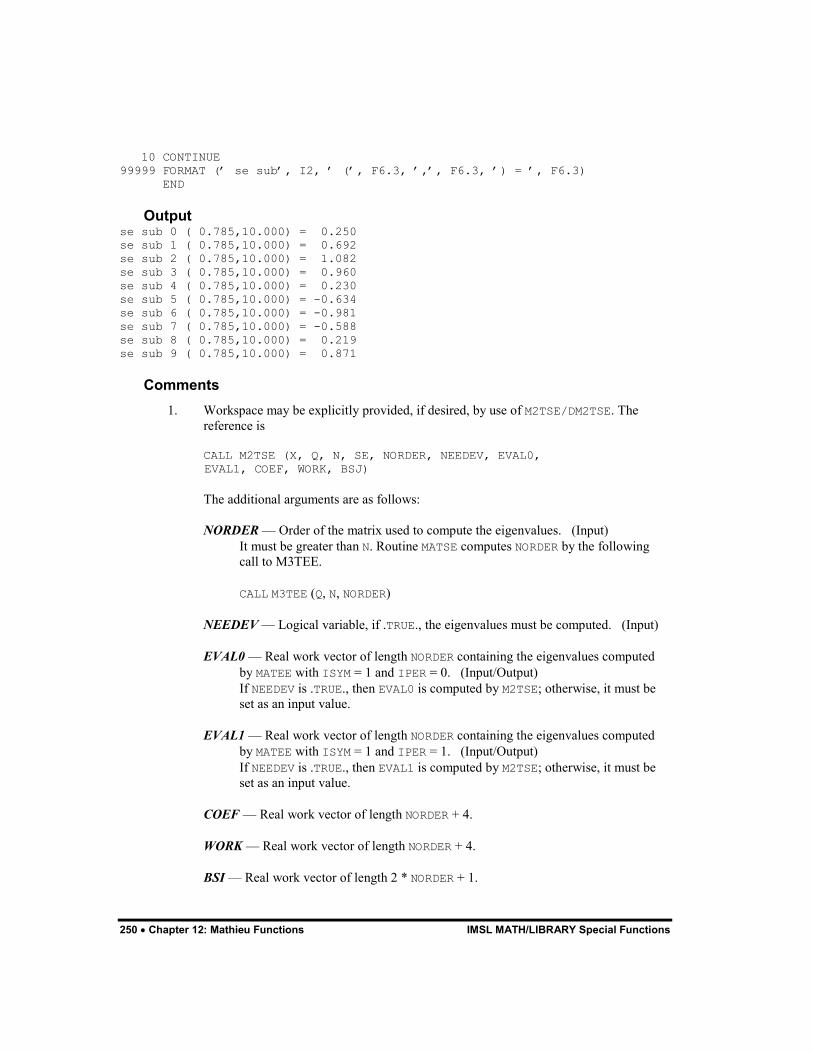
250 � Chapter 12: Mathieu Functions IMSL MATH/LIBRARY Special Functions
10 CONTINUE 99999 FORMAT (’ se sub’, I2, ’ (’, F6.3, ’,’, F6.3, ’) = ’, F6.3) END
Output se sub 0 ( 0.785,10.000) = 0.250 se sub 1 ( 0.785,10.000) = 0.692 se sub 2 ( 0.785,10.000) = 1.082 se sub 3 ( 0.785,10.000) = 0.960 se sub 4 ( 0.785,10.000) = 0.230 se sub 5 ( 0.785,10.000) = -0.634 se sub 6 ( 0.785,10.000) = -0.981 se sub 7 ( 0.785,10.000) = -0.588 se sub 8 ( 0.785,10.000) = 0.219 se sub 9 ( 0.785,10.000) = 0.871
Comments 1. Workspace may be explicitly provided, if desired, by use of M2TSE/DM2TSE. The
reference is
CALL M2TSE (X, Q, N, SE, NORDER, NEEDEV, EVAL0, EVAL1, COEF, WORK, BSJ)
The additional arguments are as follows:
NORDER — Order of the matrix used to compute the eigenvalues. (Input) It must be greater than N. Routine MATSE computes NORDER by the following call to M3TEE.
CALL M3TEE (Q, N, NORDER)
NEEDEV — Logical variable, if .TRUE., the eigenvalues must be computed. (Input)
EVAL0 — Real work vector of length NORDER containing the eigenvalues computed by MATEE with ISYM = 1 and IPER = 0. (Input/Output) If NEEDEV is .TRUE., then EVAL0 is computed by M2TSE; otherwise, it must be set as an input value.
EVAL1 — Real work vector of length NORDER containing the eigenvalues computed by MATEE with ISYM = 1 and IPER = 1. (Input/Output) If NEEDEV is .TRUE., then EVAL1 is computed by M2TSE; otherwise, it must be set as an input value.
COEF — Real work vector of length NORDER + 4.
WORK — Real work vector of length NORDER + 4.
BSI — Real work vector of length 2 * NORDER + 1.

IMSL MATH/LIBRARY Special Functions Chapter 12: Mathieu Functions � 251
2. Informational error Type Code
4 1 The iteration for the eigenvalues did not converge.
Description The eigenvalues of Mathieu’s equation are computed using MATEE (page 241). The function values are then computed using a sum of Bessel functions, see Gradshteyn and Ryzhik (1965), equation 8.661.

252 � Chapter 12: Mathieu Functions IMSL MATH/LIBRARY Special Functions
IMSL MATH/LIBRARY Special Functions Chapter 13: Miscellaneous Functions � 253
Chapter 13: Miscellaneous Functions
Routines Spence dilogarithm ..............................................................SPENC 255 Initialize a Chebyshev series ..................................................INITS 256 Evaluate a Chebyshev series .............................................. CSEVL 257
Usage Notes Many functions of one variable can be numerically computed using a Chebyshev series,
� � � �01 1n nn
f x A T x x�
�
� � � ��
A Chebyshev series is better for numerical computation than a Taylor series since the Chebyshev polynomials, Tn(x), are better behaved than the monomials, xn.
A Taylor series can be converted into a Chebyshev series using an algorithm of Fields and Wimp, (see Luke (1969), page 292).
Let
� � 0n
nnf x x�
�
�
��
be a Taylor series expansion valid for |x| < 1. Define
� � � �
� �
12
0
122 1 !4
n kkkn n k
k
n nA
n k�
� �
�
� �
�
��
where (a)k = (a + k)/(a) is Pochhammer’s symbol.
254 � Chapter 13: Miscellaneous Functions IMSL MATH/LIBRARY Special Functions
(Note that (a)k���� = (a + k)(a)k). Then,
� � � � � �* *102 1
0 1n nnf x T x A T x x�
�
� � � ��
where
� �*nT x
are the shifted Chebyshev polynomials,
� � � �* * 2 1n nT x T x� �
In an actual implementation of this algorithm, the number of terms in the Taylor series and the number of terms in the Chebyshev series must both be finite. If the Taylor series is an alternating series, then the error in using only the first M terms is less than |�M � � |. The error in truncating the Chebyshev series to N terms is no more than
1 nn Nc�
� ��
If the Taylor series is valid on |x| < R, then we can write
� � � �0/ nn
nnf x R x R�
�
�
��
and use �nRn instead of �n in the algorithm to obtain a Chebyshev series in x/R valid for 0 < x < R. Unfortunately, if R is large, then the Chebyshev series converges more slowly.
The Taylor series centered at zero can be shifted to a Taylor series centered at c. Let t = x � c, so
� � � � � �
� �
0 0 0
0 0ˆ ˆ
nn n j jn nn n j
nnn nn n
nf x f t c t c c t
j
t x c
� �
� �
� ��
� � �
� �
� �
� �� � � � � � �
� �
� �
� � �
� �
By interchanging the order of the double sum, it can easily be shown that
ˆ n jj nn j
nc
j� �
��
�
� �� � �
� ��
By combining scaling and shifting, we can obtain a Chebyshev series valid over any interval [a, b] for which the original Taylor series converges.
The algorithm can also be applied to asymptotic series,
� � 0~ as n
nnf x x x�
��
�
���
by treating the series truncated to M terms as a polynomial in 1/x. The asymptotic series is usually divergent; but if it is alternating, the error in truncating the series to M terms is less than |�M �
�|/RM � � for R � x < �. Normally, as M increases, the error initially decreases to a small value and then increases without a bound. Therefore, there is a limit to the accuracy that can be obtained by increasing M. More accuracy can be obtained by increasing R. The optimal value of M depends on
IMSL MATH/LIBRARY Special Functions Chapter 13: Miscellaneous Functions � 255
both the sequence �j and R. For R fixed, the optimal value of M can be found by finding the value
of M at which |�M|/RM starts to increase.
Since we want a routine accurate to near machine precision, the algorithm must be implemented using somewhat higher precision than is normally used. This is best done using a symbolic computation package.
SPENC This function evaluates a form of Spence’s integral.
Function Return Value SPENC — Function value. (Output)
Required Arguments X — Argument for which the function value is desired. (Input)
FORTRAN 90 Interface Generic: SPENC (X)
Specific: The specific interface names are S_SPENC and D_SPENC.
FORTRAN 77 Interface Single: SPENC (X)
Double: The double precision function name is DSPENC.
Example In this example, s(0.2) is computed and printed.
USE SPENC_INT USE UMACH_INT ! Declare variables INTEGER NOUT REAL VALUE, X ! Compute X = 0.2 VALUE = SPENC(X) ! Print the results CALL UMACH (2, NOUT) WRITE (NOUT,99999) X, VALUE 99999 FORMAT (’ SPENC(’, F6.3, ’) = ’, F6.3) END
256 � Chapter 13: Miscellaneous Functions IMSL MATH/LIBRARY Special Functions
Output SPENC( 0.200) = 0.211
Description The Spence dilogarithm function, s(x), is defined to be
� �0
ln 1x ys x dy
y�
� ��
For |x| � 1, the uniformly convergent expansion
� � 21
k
k
xs xk
�
�
��
is valid.
Spence’s function can be used to evaluate much more general integral forms. For example,
� � � � � �0
loglog
z ax b a cz d a cz dc dx s
cx d ad bc ad bc� � �� �
� � � �� � ��
�
INITS This function Initializes the orthogonal series so the function value is the number of terms needed to insure the error is no larger than the requested accuracy.
Function Return Value INITS — Number of terms needed to insure the error is no larger than ETA. (Output)
Required Arguments OS — Vector of length NOS containing coefficients in an orthogonal series. (Input)
NOS — Number of coefficients in OS. (Input)
ETA — Requested accuracy of the series. (Input) Contrary to the usual convention, ETA is a REAL argument to INITDS.
FORTRAN 90 Interface Generic: INITS(OS, NOS, ETA)
Specific: The specific interface names are INITS and INITDS.
FORTRAN 77 Interface Single: INITS(OS, NOS, ETA)
IMSL MATH/LIBRARY Special Functions Chapter 13: Miscellaneous Functions � 257
Double: The double precision function name is INITDS.
Comments ETA will usually be chosen to be one tenth of machine precision.
Description Function INITS initializes a Chebyshev series. The function INITS returns the number of terms in the series s of length n needed to insure that the error of the evaluated series is everywhere less than ETA. The number of input terms n must be greater than 1, so that a series of at least one term and an error estimate can be obtained. In addition, ETA should be larger than the absolute value of the last coefficient. If it is not, then all the terms of the series must be used, and no error estimate is available.
CSEVL This function evaluates the N-term Chebyshev series.
Function Return Value CSEVL — Function value. (Output)
Required Arguments X — Argument at which the series is to be evaluated. (Input)
CS — Vector of length N containing the terms of a Chebyshev series. (Input) In evaluating CS, only half of the first coefficient is summed.
Optional Arguments N — Number of terms in the vector CS. (Input)|
Default: N = size(CS, 1)
FORTRAN 90 Interface Generic: CSEVL(X, CS [,…])
Specific: The specific interface names are S_CSEVL and D_CSEVL.
FORTRAN 77 Interface Single: CSEVL(X, CS, N)
Double: The double precision function name is DCSEVL.
258 � Chapter 13: Miscellaneous Functions IMSL MATH/LIBRARY Special Functions
Comments Informational error Type Code
3 7 X is outside the interval (�1.1, +1.1)
Description Function CSEVL evaluates a Chebyshev series whose coefficients are stored in the array s of length n at the point x. The argument x must lie in the interval [�1, +1]. Other finite intervals can be linearly transformed to this canonical interval. Also, the number of terms in the series must be greater than zero but less than 1000. This latter limit is purely arbitrary; it is imposed in order to guard against the possibility of a floating point number being passed as an argument for n.
IMSL MATH/LIBRARY Special Functions Reference Material � 259
Reference Material
User Errors.................................................................................259 Machine-Dependent Constants ................................................. 263 Reserved Names .......................................................................263 Deprecated and Deleted Routines ............................................ 270 Automatic Workspace Allocation ...............................................270
User Errors IMSL routines attempt to detect user errors and handle them in a way that provides as much in-formation to the user as possible. To do this, we recognize various levels of severity of errors, and we also consider the extent of the error in the context of the purpose of the routine; a trivial error in one situation may be serious in another. IMSL routines attempt to report as many errors as they can reasonably detect. Multiple errors present a difficult problem in error detection because input is interpreted in an uncertain context after the first error is detected.
What Determines Error Severity In some cases, the user’s input may be mathematically correct, but because of limitations of the computer arithmetic and of the algorithm used, it is not possible to compute an answer accurately. In this case, the assessed degree of accuracy determines the severity of the error. In cases where the routine computes several output quantities, if some are not computable but most are, an error condition exists. The severity depends on an assessment of the overall impact of the error.
Terminal errors If the user’s input is regarded as meaningless, such as N = �1 when “N” is the number of equations, the routine prints a message giving the value of the erroneous input argument(s) and the reason for the erroneous input. The routine will then cause the user’s program to stop. An error in which the user’s input is meaningless is the most severe error and is called a terminal error. Multiple terminal error messages may be printed from a single routine.
Informational errors In many cases, the best way to respond to an error condition is simply to correct the input and rerun the program. In other cases, the user may want to take actions in the program itself based on errors that occur. An error that may be used as the basis for corrective action within the program is called an informational error. If an informational error occurs, a user-retrievable code is set. A
260 � Reference Material IMSL MATH/LIBRARY Special Functions
routine can return at most one informational error for a single reference to the routine. The codes for the informational error codes are printed in the error messages.
Other errors In addition to informational errors, IMSL routines issue error messages for which no user-retrievable code is set. Multiple error messages for this kind of error may be printed. These errors, which generally are not described in the documentation, include terminal errors as well as less serious errors. Corrective action within the calling program is not possible for these errors.
Kinds of Errors and Default Actions Five levels of severity of errors are defined in the MATH/LIBRARY Special Functions. Each level has an associated PRINT attribute and a STOP attribute. These attributes have default settings (YES or NO), but they may also be set by the user. The purpose of having multiple error severity levels is to provide independent control of actions to be taken for errors of different severity. Upon return from an IMSL routine, exactly one error state exists. (A code 0 “error” is no informational error.) Even if more than one informational error occurs, only one message is printed (if the PRINT attribute is YES). Multiple errors for which no corrective action within the calling program is reasonable or necessary result in the printing of multiple messages (if the PRINT attribute for their severity level is YES). Errors of any of the severity levels except level 5 may be informational errors.
Level 1: Note. A note is issued to indicate the possibility of a trivial error or simply to provide information about the computations. Default attributes: PRINT=NO, STOP=NO
Level 2: Alert. An alert indicates that the user should be advised about events occurring in the software. Default attributes: PRINT=NO, STOP=NO
Level 3: Warning. A warning indicates the existence of a condition that may require corrective action by the user or calling routine. A warning error may be issued because the results are accurate to only a few decimal places, because some of the output may be erroneous but most of the output is correct, or because some assumptions underlying the analysis technique are violated. Often no corrective action is necessary and the condition can be ignored. Default attributes: PRINT=YES, STOP=NO
Level 4: Fatal. A fatal error indicates the existence of a condition that may be serious. In most cases, the user or calling routine must take corrective action to recover. Default attributes: PRINT=YES, STOP=YES
Level 5: Terminal. A terminal error is serious. It usually is the result of an incorrect specification, such as specifying a negative number as the number of equations. These errors may also be caused by various programming errors impossible to diagnose correctly in FORTRAN. The resulting error message may be perplexing to the user. In such cases, the user is advised to compare carefully the actual arguments passed to the routine with the dummy argument descriptions given in the documentation. Special attention should be given to checking argument order and data types.

IMSL MATH/LIBRARY Special Functions Reference Material � 261
A terminal error is not an informational error because corrective action within the program is generally not reasonable. In normal usage, execution is terminated immediately when a terminal error occurs. Messages relating to more than one terminal error are printed if they occur. Default attributes: PRINT=YES, STOP=YES
The user can set PRINT and STOP attributes by calling ERSET as described in “Routines for Error Handling.”
Errors in Lower-Level Routines It is possible that a user’s program may call an IMSL routine that in turn calls a nested sequence of lower-level IMSL routines. If an error occurs at a lower level in such a nest of routines and if the lower-level routine cannot pass the information up to the original user-called routine, then a traceback of the routines is produced. The only common situation in which this can occur is when an IMSL routine calls a user-supplied routine that in turn calls another IMSL routine.
Routines for Error Handling There are three ways in which the user may interact with the IMSL error handling system: (1) to change the default actions, (2) to retrieve the integer code of an informational error so as to take corrective action, and (3) to determine the severity level of an error. The routines to use are ERSET, IERCD, and N1RTY, respectively.
ERSET Change the default printing or stopping actions when errors of a particular error severity level occur.
Required Arguments IERSVR — Error severity level indicator. (Input)
If IERSVR = 0, actions are set for levels 1 to 5. If IERSVR is 1 to 5, actions are set for errors of the specified severity level.
IPACT — Printing action. (Input)
IPACT Action
�1 Do not change current setting(s).
0 Do not print.
1 Print.
2 Restore the default setting(s).
ISACT — Stopping action. (Input)
ISACT Action
�1 Do not change current setting(s).
262 � Reference Material IMSL MATH/LIBRARY Special Functions
0 Do not stop.
1 Stop.
2 Restore the default setting(s).
FORTRAN 90 Interface Generic: CALL ERSET (IERSVR, IPACT, ISACT)
Specific: The specific interface name is ERSET.
FORTRAN 77 Interface Single: CALL ERSET (IERSVR, IPACT, ISACT)
IERCD and N1RTY The last two routines for interacting with the error handling system, IERCD and N1RTY, are INTEGER functions and are described in the following material.
IERCD retrieves the integer code for an informational error. Since it has no arguments, it may be used in the following way:
ICODE = IERCD( )
The function retrieves the code set by the most recently called IMSL routine.
N1RTY retrieves the error type set by the most recently called IMSL routine. It is used in the following way:
ITYPE = N1RTY(1)
ITYPE = 1, 2, 4, and 5 correspond to error severity levels 1, 2, 4, and 5, respectively. ITYPE = 3 and ITYPE = 6 are both warning errors, error severity level 3. While ITYPE = 3 errors are informational errors (IERCD( ) � 0), ITYPE = 6 errors are not informational errors (IERCD( ) = 0).
For software developers requiring additional interaction with the IMSL error handling system, see Aird and Howell (1991).
Examples
Changes to Default Actions Some possible changes to the default actions are illustrated below. The default actions remain in effect for the kinds of errors not included in the call to ERSET.
To turn off printing of warning error messages: CALL ERSET (3, 0, �1)
To stop if warning errors occur: CALL ERSET (3, �1, 1)
IMSL MATH/LIBRARY Special Functions Reference Material � 263
To print all error messages: CALL ERSET (0, 1, �1)
To restore all default settings: CALL ERSET (0, 2, 2)
Machine-Dependent Constants The function subprograms in this section return machine-dependent information and can be used to enhance portability of programs between different computers. The routines IMACH, and AMACH describe the computer’s arithmetic. The routine UMACH describes the input, ouput, and error output unit numbers.
IMACH
This function retrieves machine integer constants that define the arithmetic used by the computer.
Function Return Value IMACH(1) = Number of bits per integer storage unit.
IMACH(2) = Number of characters per integer storage unit:
Integers are represented in M-digit, base A form as
0
M kkk
x A��
�
where is the sign and 0 � xk < A, k = 0, �, M.
Then,
IMACH(3) = A, the base.
IMACH(4) = M, the number of base-A digits.
IMACH(5) = AM � 1, the largest integer.
The machine model assumes that floating-point numbers are represented in normalized N-digit, base B form as
1
NE kkk
B x B��
��
where is the sign, 0 < x� < B, 0 � xk < B, k = 2, �, N and E� � E � E�. Then,
264 � Reference Material IMSL MATH/LIBRARY Special Functions
min
IMACH(6) = , the base.IMACH(7) = , the number of base- digits in single precision.IMACH(8) = , the smallest single precision exponent.
s
s
BN BE
max
min
max
IMACH(9) = , the largest single precision exponent.
IMACH(10) = , the number of base- digits in double precision.IMACH(11) = , the smallest double precision exponent.
IMACH(12) = , the
s
d
d
d
E
N BE
E number of base- digits in double precisionB
Required Arguments I — Index of the desired constant. (Input)
FORTRAN 90 Interface Generic: IMACH (I)
Specific: The specific interface name is IMACH.
FORTRAN 77 Interface Single: IMACH (I)
AMACH
The function subprogram AMACH retrieves machine constants that define the computer’s single-precision or double precision arithmetic. Such floating-point numbers are represented in normalized N-digit, base B form as
1
NE kkk
B x B��
��
where is the sign, 0 < x� < B, 0 � xk < B, k = 2, �, N and
min maxE E E� �
Function Return Value
� �
AMACH(1)
AMACH(2)
AMACH(3)
AMACH(4)
1min , the smallest normalized positive number.
max= 1 , the largest number.
= , the smallest relative spacing.1= , the largest relative spacing.
EBE NB B
NBNB
�
�
��
�
�
IMSL MATH/LIBRARY Special Functions Reference Material � 265
� �AMACH(5)
AMACH(6)
AMACH(7)
AMACH(8)
= log .10NaN (non-signaling not a number).
=positive machine infinity.= negative machine infinity.
B
�
See Comment 1 for a description of the use of the generic version of this function.
See Comment 2 for a description of min, max, and N.
Required Arguments I — Index of the desired constant. (Input)
FORTRAN 90 Interface Generic: AMACH (I)
Specific: The specific interface names are S_AMACH and D_AMACH.
FORTRAN 77 Interface Single: AMACH (I)
Double: The double precision name is DMACH.
Comments 1. If the generic version of this function is used, the immediate result must be stored in a
variable before use in an expression. For example:
X = AMACH(I) Y = SQRT(X) must be used rather than
Y = SQRT(AMACH(I)).
If this is too much of a restriction on the programmer, then the specific name can be used without this restriction..
2. Note that for single precision B = IMACH(6), N = IMACH(7). Emin = IMACH(8), and Emax = IMACH(9). For double precision B = IMACH(6), N = IMACH(10). Emin = IMACH(11), and Emax = IMACH(12).
266 � Reference Material IMSL MATH/LIBRARY Special Functions
3. The IEEE standard for binary arithmetic (see IEEE 1985) specifies quiet NaN (not a number) as the result of various invalid or ambiguous operations, such as 0/0. The intent is that AMACH(6) return a quiet NaN. On IEEE format computers that do not support a quiet NaN, a special value near AMACH(2) is returned for AMACH(6). On computers that do not have a special representation for infinity, AMACH(7) returns the same value as AMACH(2).
DMACH
See AMACH.
IFNAN(X) This logical function checks if the argument X is NaN (not a number).
Function Return Value IFNAN - Logical function value. True is returned if the input argument is a NAN. Otherwise,
False is returned. (Output)
Required Arguments X – Argument for which the test for NAN is desired. (Input)
FORTRAN 90 Interface Generic: IFNAN(X)
Specific: The specific interface names are S_IFNAN and D_IFNAN.
FORTRAN 77 Interface Single: IFNAN (X)
Double: The double precision name is DIFNAN.
Example USE IFNAN_INT USE AMACH_INT USE UMACH_INT INTEGER NOUT REAL X ! CALL UMACH (2, NOUT) ! X = AMACH(6)

IMSL MATH/LIBRARY Special Functions Reference Material � 267
IF (IFNAN(X)) THEN WRITE (NOUT,*) ’ X is NaN (not a number).’ ELSE WRITE (NOUT,*) ’ X = ’, X END IF ! END
Output X is NaN (not a number).
Description The logical function IFNAN checks if the single or double precision argument X is NAN (not a number). The function IFNAN is provided to facilitate the transfer of programs across computer systems. This is because the check for NaN can be tricky and not portable across computer systems that do not adhere to the IEEE standard. For example, on computers that support the IEEE standard for binary arithmetic (see IEEE 1985), NaN is specified as a bit format not equal to itself. Thus, the check is performed as IFNAN = X .NE. X
On other computers that do not use IEEE floating-point format, the check can be performed as: IFNAN = X .EQ. AMACH(6)
The function IFNAN is equivalent to the specification of the function Isnan listed in the Appendix, (IEEE 1985). The above example illustrates the use of IFNAN. If X is NaN, a message is printed instead of X. (Routine UMACH, which is described in the following section, is used to retrieve the output unit number for printing the message.)
UMACH Routine UMACH sets or retrieves the input, output, or error output device unit numbers.
Required Arguments N — Integer value indicating the action desired. If the value of N is negative, the input, output, or error output unit number is reset to NUNIT. If the value of N is positive, the input, output, or error output unit number is returned in NUNIT. See the table in argument NUNIT for legal values of N. (Input)
NUNIT — The unit number that is either retrieved or set, depending on the value of input argument N. (Input/Output)
The arguments are summarized by the following table:
N Effect 1 Retrieves input unit number in NUNIT. 2 Retrieves output unit number in NUNIT.

268 � Reference Material IMSL MATH/LIBRARY Special Functions
N Effect 3 Retrieves error output unit number in NUNIT.
�1 Sets the input unit number to NUNIT. �2 Sets the output unit number to NUNIT. �3 Sets the error output unit number to NUNIT.
FORTRAN 90 Interface Generic: CALL UMACH (N, NUNIT)
Specific: The specific interface name is UMACH.
FORTRAN 77 Interface Single: CALL UMACH (N, NUNIT)
Example In the following example, a terminal error is issued from the MATH/LIBRARY AMACH function since the argument is invalid. With a call to UMACH, the error message will be written to a local file named “CHECKERR”.
USE AMACH_INT USE UMACH_INT
INTEGER N, NUNIT REAL X ! Set Parameter N = 0 ! NUNIT = 9 CALL UMACH (-3, NUNIT) OPEN (UNIT=9,FILE=’CHECKERR’) X = AMACH(N) END
Output The output from this example, written to “CHECKERR” is:
*** TERMINAL ERROR 5 from AMACH. The argument must be between 1 and 8 *** inclusive. N = 0
Description Routine UMACH sets or retrieves the input, output, or error output device unit numbers. UMACH is set automatically so that the default FORTRAN unit numbers for standard input, standard output, and standard error are used. These unit numbers can be changed by inserting a call to UMACH at the beginning of the main program that calls MATH/LIBRARY routines. If these unit numbers are
IMSL MATH/LIBRARY Special Functions Reference Material � 269
changed from the standard values, the user should insert an appropriate OPEN statement in the calling program.
Reserved Names When writing programs accessing IMSL MATH/LIBRARY Special Functions, the user should choose FORTRAN names that do not conflict with names of IMSL subroutines, functions, or named common blocks, such as the workspace common block WORKSP (page 261). The user needs to be aware of two types of name conflicts that can arise. The first type of name conflict occurs when a name (technically a symbolic name) is not uniquely defined within a program unit (either a main program or a subprogram). For example, such a name conflict exists when the name BSJS is used to refer both to a type REAL variable and to the IMSL routine BSJS in a single program unit. Such errors are detected during compilation and are easy to correct. The second type of name conflict, which can be more serious, occurs when names of program units and named common blocks are not unique. For example, such a name conflict would be caused by the user defining a routine named WORKSP and also referencing a MATH/LIBRARY Special Functions routine that uses the named common block WORKSP. Likewise, the user must not define a subprogram with the same name as a subprogram in MATH/LIBRARY Special Functions, that is referenced directly by the user’s program or is referenced indirectly by other MATH/LIBRARY Special Functions subprograms.
MATH/LIBRARY Special Functions consists of many routines, some that are described in the User’s Manual and others that are not intended to be called by the user and, hence, that are not documented. If the choice of names were completely random over the set of valid FORTRAN names and if a program uses only a small subset of MATH/LIBRARY Special Functions, the probability of name conflicts is very small. Since names are usually chosen to be mnemonic, however, the user may wish to take some precautions in choosing FORTRAN names.
Many IMSL names consist of a root name that may have a prefix to indicate the type of the routine. For example, the IMSL single precision routine for computing Bessel functions of the first kind with real order has the name BSJS, which is the root name, and the corresponding IMSL double precision routine has the name DBSJS. Associated with these two routines are B2JS and DB2JS. BSJS is listed in the Alphabetical Index of Routines, but DBSJS, B2JS, and DB2JS are not. The user of BSJS must consider both names BSJS and B2JS to be reserved; likewise, the user of DBSJS must consider both names DBSJS and DB2JS to be reserved. The root names of all routines and named common blocks that are used by MATH/LIBRARY Special Functions and that do not have a numeral in the second position of the root name are listed in the Alphabetical Index of Routines. Some of the routines in this Index are not intended to be called by the user and so are not documented. The careful user can avoid any conflicts with IMSL names if the following rules are observed:
� Do not choose a name that appears in the Alphabetical Summary of Routines in the User’s Manual, nor one of these names preceded by a D, S_, D_, C_, or Z_.
� Do not choose a name of three or more characters with a numeral in the second or third position.
These simplified rules include many combinations that are, in fact, allowable. However, if the user selects names that conform to these rules, no conflict will be encountered.
270 � Reference Material IMSL MATH/LIBRARY Special Functions
Deprecated Features and Deleted Routines Automatic Workspace Allocation FORTRAN subroutines that work with arrays as input and output often require extra arrays for use as workspace while doing computations or moving around data. IMSL routines generally do not require the user explicitly to allocate such arrays for use as workspace. On most systems the workspace allocation is handled transparently. The only limitation is the actual amount of memory available on the system.
On some systems the workspace is allocated out of a stack that is passed as a FORTRAN array in a named common block WORKSP. A very similar use of a workspace stack is described by Fox et al. (1978, pages 116�121). (For compatiblity with older versions of the IMSL Libraries, space is allocated from the COMMON block, if possible.)
The arrays for workspace appear as arguments in lower-level routines. For example, the IMSL routine LSARG (in Chapter 1, “Linear Systems”), which solves systems of linear equations, needs arrays for workspace. LSARG allocates arrays from the common area, and passes them to the lower-level routine L2ARG which does the computations. In the “Comments” section of the documentation for LSARG, the amount of workspace is noted and the call to L2ARG is described. This scheme for using lower-level routines is followed throughout the IMSL Libraries. The names of these routines have a “2” in the second position (or in the third position in double precision routines having a “D” prefix). The user can provide workspace explicitly and call directly the “2-level” routine, which is documented along with the main routine. In a very few cases, the 2-level routine allows additional options that the main routine does not allow.
Prior to returning to the calling program, a routine that allocates workspace generally deallocates that space so that it becomes available for use in other routines.
Changing the Amount of Space Allocated This section is relevant only to those systems on which the transparent workspace allocator is not available.
By default, the total amount of space allocated in the common area for storage of numeric data is 5000 numeric storage units. (A numeric storage unit is the amount of space required to store an integer or a real number. By comparison, a double precision unit is twice this amount. Therefore, the total amount of space allocated in the common area for storage of numeric data is 2500 double precision units.) This space is allocated as needed for INTEGER, REAL, or other numeric data. For larger problems in which the default amount of workspace is insufficient, the user can change the allocation by supplying the FORTRAN statements to define the array in the named common block and by informing the IMSL workspace allocation system of the new size of the common array. To request 7000 units, the statements are
COMMON /WORKSP/ RWKSP REAL RWKSP(7000) CALL IWKIN(7000)
If an IMSL routine attempts to allocate workspace in excess of the amount available in the com-mon stack, the routine issues a fatal error message that indicates how much space is needed and prints statements like those above to guide the user in allocating the necessary amount. The

IMSL MATH/LIBRARY Special Functions Reference Material � 271
program below uses IMSL routine BSJS (See Chapter 6, “Bessel Funtions ” of this manual.) to illustrate this feature.
This routine requires workspace that is just larger than twice the number of function values requested.
INTEGER N REAL BS(10000), X, XNU EXTERNAL BSJS ! Set Parameters XNU = .5 X = 1. N = 6000 CALL BSJS (XNU, X, N, BS) END
Output *** TERMINAL ERROR from BSJS. Insufficient workspace for *** current allocation(s). Correct by calling *** IWKIN from main program with the three *** following statements: (REGARDLESS OF *** PRECISION) *** COMMON /WORKSP/ RWKSP *** REAL RWKSP(12018) *** CALL IWKIN(12018)
*** TERMINAL ERROR from BSJS. The workspace requirement is *** based on N =6000. STOP
In most cases, the amount of workspace is dependent on the parameters of the problem so the amount needed is known exactly. In a few cases, however, the amount of workspace is dependent on the data (for example, if it is necessary to count all of the unique values in a vector). Thus, the IMSL routine cannot tell in advance exactly how much workspace is needed. In such cases, the error message printed is an estimate of the amount of space required.
Character Workspace Since character arrays cannot be equivalenced with numeric arrays, a separate named common block WKSPCH is provided for character workspace. In most respects, this stack is managed in the same way as the numeric stack. The default size of the character workspace is 2000 character units. (A character unit is the amount of space required to store one character.) The routine analogous to IWKIN used to change the default allocation is IWKCIN.
The routines in the following list are being deprecated in Version 2.0 of MATH/LIBRARY Special Functions. A deprecated routine is one that is no longer used by anything in the library but is being included in the product for those users who may be currently referencing it in their application. However, any future versions of MATH/LIBRARY Special Functions will not include these routines. If any of these routines are being called within an application, it is recommended that you change your code or retain the deprecated routine before replacing this library with the next version. Most of these routines were called by users only when they needed to set up their own workspace. Thus, the impact of these changes should be limited.
272 � Reference Material IMSL MATH/LIBRARY Special Functions
G2DF G2IN G3DF
The following specific FORTRAN intrinsic functions are no longer supplied by IMSL. They can all be found in their manufacturer’s FORTRAN runtime libraries. If any change must be made to the user’s application as a result of their removal from the IMSL Libraries, it is limited to the redeclaration of the function from “external” to “intrinsic.” Argument lists and results should be identical.
ACOS CEXP DATAN2 DSQRT
AINT CLOG DCOS DTAN
ALOG COS DCOSH DTANH
ALOG10 COSH DEXP EXP
ASIN CSIN DINT SIN
ATAN CSQRT DLOG SINH
ATAN2 DACOS DLOG10 SQRT
CABS DASIN DSIN TAN
CCOS DATAN DSINH TANH
IMSL MATH/LIBRARY Special Functions GAMS Index � A-1
GAMS Index
Description This index lists routines in MATH/LIBRARY Special Functions by a tree-structured classification scheme known as GAMS. Boisvert, Howe, Kahaner, and Springmann (1990) give the GAMS classification scheme. The classification scheme given here is Version 2.0. The first level of the classification scheme is denoted by a letter A thru Z as follows: A. Arithmetic, Error Analysis B. Number Theory C. Elementary and Special Functions D. Linear Algebra E. Interpolation F. Solution of Nonlinear Equations G. Optimization H. Differentiation and Integration I. Differential and Integral Equations J. Integral Transforms K. Approximation L. Statistics, Probability M. Simulation, Stochastic Modeling N. Data Handling O. Symbolic Computation P. Computational Geometry Q. Graphics R. Service Routines S. Software Development Tools Z. Other
There are seven levels in the classification scheme. Subclasses for levels 3, 5, and 7 are denoted by letters �a� thru �w�. Subclasses for levels 2, 4, and 6 are denoted by the numbers 1 thru 23.
The index given in the following pages lists routines in MATH/LIBRARY Special Functions within each GAMS subclass. The purpose of the routine appear alongside the routine name.
A-2 � GAMS Index IMSL MATH/LIBRARY Special Functions
IMSL MATH/LIBRARY Special Functions C...........ELEMENTARY AND SPECIAL FUNCTIONS (search also class L5)
C1.........Integer-valued functions (e.g., floor, ceiling, factorial, binomial coefficient)
BINOM Evaluates the binomial coefficient. FAC Evaluates the factorial of the argument.
C2.........Powers, roots, reciprocals CBRT Evaluates the real or complex cube root.
C3.........Polynomials
C3a .......Orthogonal INITS Initializes the orthogonal series so the function value is the
number of terms needed to insure the error is no larger than the requested accuracy.
C3a2 .....Chebyshev, Legendre CSEVL Evaluates the N-term Chebyshev series.
C4.........Elementary transcendental functions CACOS Evaluates the complex arc cosine. CARG Evaluates the argument of a complex number. CASIN Evaluates the complex arc sine. CATAN Evaluates the complex arc tangent. CATAN2 Evaluates the complex arc tangent of a ratio. COSDG Evaluates the cosine for the argument in degrees. COT Evaluates the real or complex cotangent. SINDG Evaluates the sine for the argument in degrees.
C4b.......Exponential, logarithmic ALNREL Evaluates the natural logarithm of one plus the argument. CLNREL Evaluates the principal value of the complex natural
logarithm of one plus the argument. EXPRL Evaluates the real or complex exponential function
factored from first order. LOG10 Evaluates the principal value of the real or complex
common logarithm.
C4c .......Hyperbolic, inverse hyperbolic ACOSH Evaluates the real or complex arc hyperbolic cosine. ASINH Evaluates the real or complex arc hyperbolic sine. ATANH Evaluates the arc hyperbolic tangent.. CSINH Evaluates the complex hyperbolic sine. CTANH Evaluates the complex hyperbolic tangent. TAN Evaluates the real or complex tangent.
C5.........Exponential and logarithmic integrals ALI Evaluates the logarithmic integral.
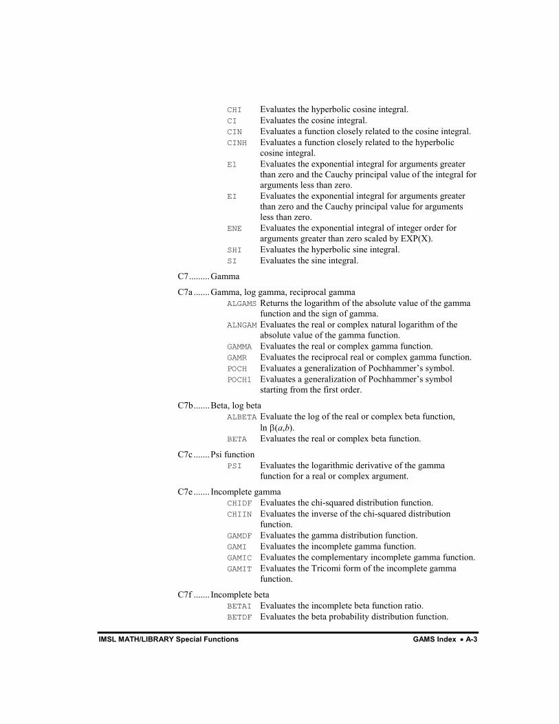
IMSL MATH/LIBRARY Special Functions GAMS Index � A-3
CHI Evaluates the hyperbolic cosine integral. CI Evaluates the cosine integral. CIN Evaluates a function closely related to the cosine integral. CINH Evaluates a function closely related to the hyperbolic
cosine integral. E1 Evaluates the exponential integral for arguments greater
than zero and the Cauchy principal value of the integral for arguments less than zero.
EI Evaluates the exponential integral for arguments greater than zero and the Cauchy principal value for arguments less than zero.
ENE Evaluates the exponential integral of integer order for arguments greater than zero scaled by EXP(X).
SHI Evaluates the hyperbolic sine integral. SI Evaluates the sine integral.
C7.........Gamma
C7a .......Gamma, log gamma, reciprocal gamma ALGAMS Returns the logarithm of the absolute value of the gamma
function and the sign of gamma. ALNGAM Evaluates the real or complex natural logarithm of the
absolute value of the gamma function. GAMMA Evaluates the real or complex gamma function. GAMR Evaluates the reciprocal real or complex gamma function. POCH Evaluates a generalization of Pochhammer�s symbol. POCH1 Evaluates a generalization of Pochhammer�s symbol
starting from the first order.
C7b.......Beta, log beta ALBETA Evaluate the log of the real or complex beta function,
ln �(a,b). BETA Evaluates the real or complex beta function.
C7c .......Psi function PSI Evaluates the logarithmic derivative of the gamma
function for a real or complex argument.
C7e ....... Incomplete gamma CHIDF Evaluates the chi-squared distribution function. CHIIN Evaluates the inverse of the chi-squared distribution
function. GAMDF Evaluates the gamma distribution function. GAMI Evaluates the incomplete gamma function. GAMIC Evaluates the complementary incomplete gamma function. GAMIT Evaluates the Tricomi form of the incomplete gamma
function.
C7f ....... Incomplete beta BETAI Evaluates the incomplete beta function ratio. BETDF Evaluates the beta probability distribution function.
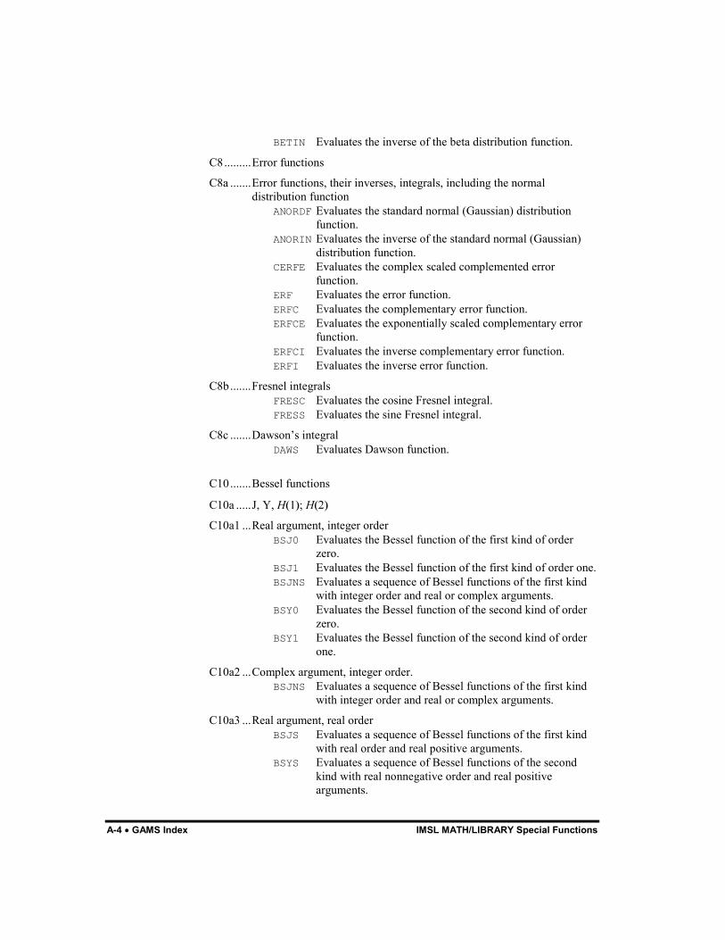
A-4 � GAMS Index IMSL MATH/LIBRARY Special Functions
BETIN Evaluates the inverse of the beta distribution function.
C8.........Error functions
C8a .......Error functions, their inverses, integrals, including the normal distribution function
ANORDF Evaluates the standard normal (Gaussian) distribution function.
ANORIN Evaluates the inverse of the standard normal (Gaussian) distribution function.
CERFE Evaluates the complex scaled complemented error function.
ERF Evaluates the error function. ERFC Evaluates the complementary error function. ERFCE Evaluates the exponentially scaled complementary error
function. ERFCI Evaluates the inverse complementary error function. ERFI Evaluates the inverse error function.
C8b.......Fresnel integrals FRESC Evaluates the cosine Fresnel integral. FRESS Evaluates the sine Fresnel integral.
C8c .......Dawson�s integral DAWS Evaluates Dawson function.
C10.......Bessel functions
C10a .....J, Y, H���; H���
C10a1 ...Real argument, integer order BSJ0 Evaluates the Bessel function of the first kind of order
zero. BSJ1 Evaluates the Bessel function of the first kind of order one. BSJNS Evaluates a sequence of Bessel functions of the first kind
with integer order and real or complex arguments. BSY0 Evaluates the Bessel function of the second kind of order
zero. BSY1 Evaluates the Bessel function of the second kind of order
one.
C10a2 ...Complex argument, integer order. BSJNS Evaluates a sequence of Bessel functions of the first kind
with integer order and real or complex arguments.
C10a3 ...Real argument, real order BSJS Evaluates a sequence of Bessel functions of the first kind
with real order and real positive arguments. BSYS Evaluates a sequence of Bessel functions of the second
kind with real nonnegative order and real positive arguments.
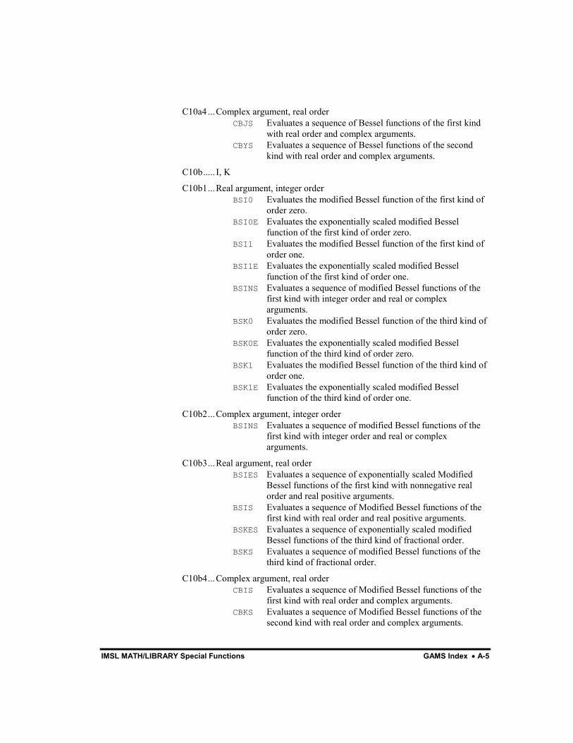
IMSL MATH/LIBRARY Special Functions GAMS Index � A-5
C10a4 ...Complex argument, real order CBJS Evaluates a sequence of Bessel functions of the first kind
with real order and complex arguments. CBYS Evaluates a sequence of Bessel functions of the second
kind with real order and complex arguments.
C10b..... I, K
C10b1...Real argument, integer order BSI0 Evaluates the modified Bessel function of the first kind of
order zero. BSI0E Evaluates the exponentially scaled modified Bessel
function of the first kind of order zero. BSI1 Evaluates the modified Bessel function of the first kind of
order one. BSI1E Evaluates the exponentially scaled modified Bessel
function of the first kind of order one. BSINS Evaluates a sequence of modified Bessel functions of the
first kind with integer order and real or complex arguments.
BSK0 Evaluates the modified Bessel function of the third kind of order zero.
BSK0E Evaluates the exponentially scaled modified Bessel function of the third kind of order zero.
BSK1 Evaluates the modified Bessel function of the third kind of order one.
BSK1E Evaluates the exponentially scaled modified Bessel function of the third kind of order one.
C10b2...Complex argument, integer order BSINS Evaluates a sequence of modified Bessel functions of the
first kind with integer order and real or complex arguments.
C10b3...Real argument, real order BSIES Evaluates a sequence of exponentially scaled Modified
Bessel functions of the first kind with nonnegative real order and real positive arguments.
BSIS Evaluates a sequence of Modified Bessel functions of the first kind with real order and real positive arguments.
BSKES Evaluates a sequence of exponentially scaled modified Bessel functions of the third kind of fractional order.
BSKS Evaluates a sequence of modified Bessel functions of the third kind of fractional order.
C10b4...Complex argument, real order CBIS Evaluates a sequence of Modified Bessel functions of the
first kind with real order and complex arguments. CBKS Evaluates a sequence of Modified Bessel functions of the
second kind with real order and complex arguments.
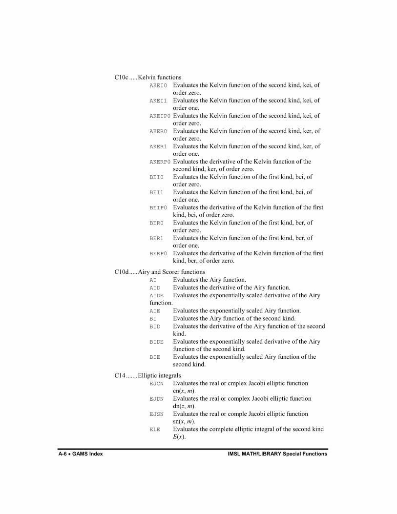
A-6 � GAMS Index IMSL MATH/LIBRARY Special Functions
C10c .....Kelvin functions AKEI0 Evaluates the Kelvin function of the second kind, kei, of
order zero. AKEI1 Evaluates the Kelvin function of the second kind, kei, of
order one. AKEIP0 Evaluates the Kelvin function of the second kind, kei, of
order zero. AKER0 Evaluates the Kelvin function of the second kind, ker, of
order zero. AKER1 Evaluates the Kelvin function of the second kind, ker, of
order one. AKERP0 Evaluates the derivative of the Kelvin function of the
second kind, ker, of order zero. BEI0 Evaluates the Kelvin function of the first kind, bei, of
order zero. BEI1 Evaluates the Kelvin function of the first kind, bei, of
order one. BEIP0 Evaluates the derivative of the Kelvin function of the first
kind, bei, of order zero. BER0 Evaluates the Kelvin function of the first kind, ber, of
order zero. BER1 Evaluates the Kelvin function of the first kind, ber, of
order one. BERP0 Evaluates the derivative of the Kelvin function of the first
kind, ber, of order zero.
C10d.....Airy and Scorer functions AI Evaluates the Airy function. AID Evaluates the derivative of the Airy function. AIDE Evaluates the exponentially scaled derivative of the Airy function. AIE Evaluates the exponentially scaled Airy function. BI Evaluates the Airy function of the second kind. BID Evaluates the derivative of the Airy function of the second
kind. BIDE Evaluates the exponentially scaled derivative of the Airy
function of the second kind. BIE Evaluates the exponentially scaled Airy function of the
second kind.
C14.......Elliptic integrals EJCN Evaluates the real or cmplex Jacobi elliptic function
cn(x, m). EJDN Evaluates the real or complex Jacobi elliptic function
dn(z, m). EJSN Evaluates the real or comple Jacobi elliptic function
sn(x, m). ELE Evaluates the complete elliptic integral of the second kind
E(x).

IMSL MATH/LIBRARY Special Functions GAMS Index � A-7
ELK Evaluates the complete elliptic integral of the kind K(x). ELRC Evaluates an elementary integral from which inverse
circular functions, logarithms and inverse hyperbolic functions can be computed.
ELRD Evaluates Carlson�s incomplete elliptic integral of the second kind RD(X, Y, Z).
ELRF Evaluates Carlson�s incomplete elliptic integral of the first kind RF(X, Y, Z).
ELRJ Evaluates Carlson�s incomplete elliptic integral of the third kind RJ(X, Y, Z, RHO).
C15.......Weierstrass elliptic functions CWPL Evaluates the Weierstrass P-function in the lemniscat case
for complex argument with unit period parallelogram. CWPLD Evaluates the first derivative of the Weierstrass P-function
in the lemniscatic case for complex argum with unit period parallelogram.
CWPQ Evaluates the Weierstrass P-function in the equianharmonic case for complex argument with unit period parallelogram.
CWPQD Evaluates the first derivative of the Weierstrass P-function in the equianharmonic case for complex argument with unit period parallelogram.
C17.......Mathieu functions MATCE Evaluates a sequence of even, periodic, integer order, real
Mathieu functions. MATEE Evaluates the eigenvalues for the periodic Mathieu
functions. MATSE Evaluates a sequence of odd, periodic, integer order, real
Mathieu functions.
C19.......Other special functions SPENC Evaluates a form of Spence�s integral.
L ...........STATISTICS, PROBABILITY
L5 .........Function evaluation (search also class C)
L5a .......Univariate
L5a1 .....Cumulative distribution functions, probability density functions GCDF Evaluates a general continuous cumulative distribution
function given ordinates of the density.
L5a1b ...Beta, binomial BETDF Evaluates the beta probability distribution function. BINDF Evaluates the binomial distribution function. BINPR Evaluates the binomial probability function.
L5a1c ...Cauchy, chi-squared CHIDF Evaluates the chi-squared distribution function. CSNDF Evaluates the noncentral chi-squared distribution function.
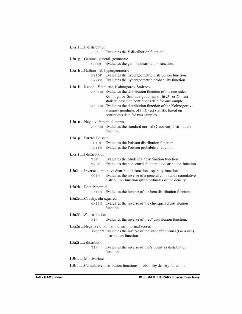
A-8 � GAMS Index IMSL MATH/LIBRARY Special Functions
L5a1f ....F distribution FDF Evaluates the F distribution function.
L5a1g ...Gamma, general, geometric GAMDF Evaluates the gamma distribution function.
L5a1h ...Halfnormal, hypergeometric HYPDF Evaluates the hypergeometric distribution function. HYPPR Evaluates the hypergeometric probability function.
L5a1k ...Kendall F statistic, Kolmogorov-Smirnov AKS1DF Evaluates the distribution function of the one-sided
Kolmogorov-Smirnov goodness of fit D� or D� test statistic based on continuous data for one sample.
AKS2DF Evaluates the distribution function of the Kolmogorov-Smirnov goodness of fit D test statistic based on continuous data for two samples.
L5a1n ...Negative binomial, normal ANORDF Evaluates the standard normal (Gaussian) distribution
function.
L5a1p ...Pareto, Poisson POIDF Evaluates the Poisson distribution function. POIPR Evaluates the Poisson probability function.
L5a1t ....t distribution TDF Evaluates the Student�s t distribution function. TNDF Evaluates the noncentral Student�s t distribution function.
L5a2 .....Inverse cumulative distribution functions, sparsity functions GCIN Evaluates the inverse of a general continuous cumulative
distribution function given ordinates of the density.
L5a2b ...Beta, binomial BETIN Evaluates the inverse of the beta distribution function.
L5a2c....Cauchy, chi-squared CHIIN Evaluates the inverse of the chi-squared distribution
function.
L5a2f ....F distribution FIN Evaluates the inverse of the F distribution function.
L5a2n ...Negative binomial, normal, normal scores ANORIN Evaluates the inverse of the standard normal (Gaussian)
distribution function.
L5a2t ....t distribution TIN Evaluates the inverse of the Student�s t distribution
function.
L5b .......Multivariate
L5b1 .....Cumulative distribution functions, probability density functions
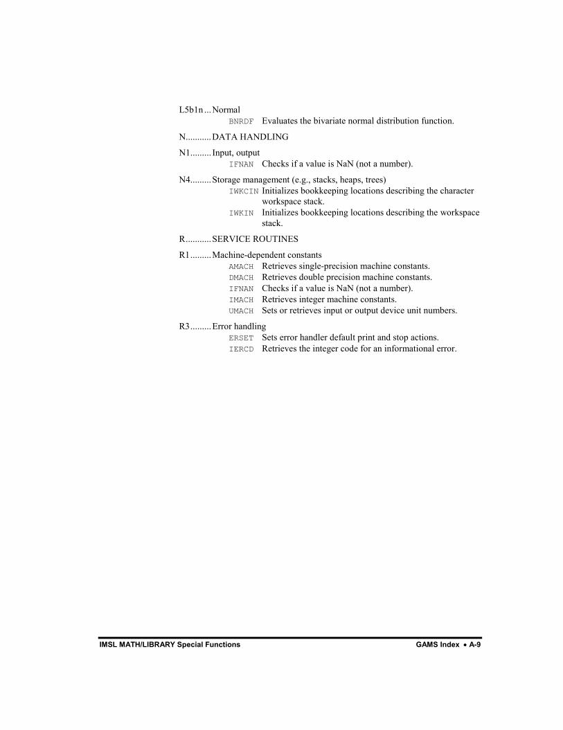
IMSL MATH/LIBRARY Special Functions GAMS Index � A-9
L5b1n ...Normal BNRDF Evaluates the bivariate normal distribution function.
N...........DATA HANDLING
N1......... Input, output IFNAN Checks if a value is NaN (not a number).
N4.........Storage management (e.g., stacks, heaps, trees) IWKCIN Initializes bookkeeping locations describing the character
workspace stack. IWKIN Initializes bookkeeping locations describing the workspace
stack.
R...........SERVICE ROUTINES
R1.........Machine-dependent constants AMACH Retrieves single-precision machine constants. DMACH Retrieves double precision machine constants. IFNAN Checks if a value is NaN (not a number). IMACH Retrieves integer machine constants. UMACH Sets or retrieves input or output device unit numbers.
R3.........Error handling ERSET Sets error handler default print and stop actions. IERCD Retrieves the integer code for an informational error.

A-10 � GAMS Index IMSL MATH/LIBRARY Special Functions
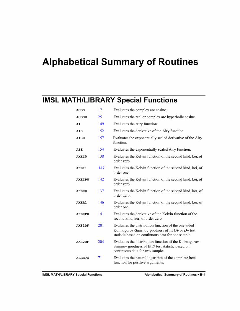
IMSL MATH/LIBRARY Special Functions Alphabetical Summary of Routines � B-1
Alphabetical Summary of Routines
IMSL MATH/LIBRARY Special Functions ACOS 17 Evaluates the complex arc cosine.
ACOSH 25 Evaluates the real or complex arc hyperbolic cosine.
AI 149 Evaluates the Airy function.
AID 152 Evaluates the derivative of the Airy function.
AIDE 157 Evaluates the exponentially scaled derivative of the Airy function.
AIE 154 Evaluates the exponentially scaled Airy function.
AKEI0 138 Evaluates the Kelvin function of the second kind, kei, of order zero.
AKEI1 147 Evaluates the Kelvin function of the second kind, kei, of order one.
AKEIP0 142 Evaluates the Kelvin function of the second kind, kei, of order zero.
AKER0 137 Evaluates the Kelvin function of the second kind, ker, of order zero.
AKER1 146 Evaluates the Kelvin function of the second kind, ker, of order one.
AKERP0 141 Evaluates the derivative of the Kelvin function of the second kind, ker, of order zero.
AKS1DF 201 Evaluates the distribution function of the one-sided Kolmogorov-Smirnov goodness of fit D� or D� test statistic based on continuous data for one sample.
AKS2DF 204 Evaluates the distribution function of the Kolmogorov-Smirnov goodness of fit D test statistic based on continuous data for two samples.
ALBETA 71 Evaluates the natural logarithm of the complete beta function for positive arguments.

B-2 � Alphabetical Summary of Routines IMSL MATH/LIBRARY Special Functions
ALGAMS 57 Returns the logarithm of the absolute value of the gamma function and the sign of gamma.
ALI 36 Evaluates the logarithmic integral.
ALNGAM 55 Evaluates the real or complex function, ln �(x)�.
ALNREL 6 Evaluates ln(x + 1) for real or complex x.
AMACH 264 Retrieves single-precision machine constants.
ANORDF 206 Evaluates the standard normal (Gaussian) distribution function.
ANORIN 208 Evaluates the inverse of the standard normal (Gaussian) distribution function.
ASIN 16 Evaluates the complex arc sine.
ASINH 24 Evaluates sinh�� x for real or complex x.
ATAN 18 Evaluates the complex arc tangent.
ATAN2 19 Evaluates the complex arc tangent of a ratio.
ATANH 27 Evaluates tanh�� x for real or complex x.
BEI0 136 Evaluates the Kelvin function of the first kind, bei, of order zero.
BEI1 145 Evaluates the Kelvin function of the first kind, bei, of order one.
BEIP0 140 Evaluates the derivative of the Kelvin function of the first kind, bei, of order zero.
BER0 135 Evaluates the Kelvin function of the first kind, ber, of order zero.
BER1 144 Evaluates the Kelvin function of the first kind, ber, of order one.
BERP0 139 Evaluates the derivative of the Kelvin function of the first kind, ber, of order zero.
BETA 69 Evaluates the real or complex beta function, �(a,b).
BETAI 73 Evaluates the incomplete beta function ratio.
BETDF 209 Evaluates the beta probability distribution function.
BETIN 212 Evaluates the inverse of the beta distribution function.
BI 150 Evaluates the Airy function of the second kind.
BID 153 Evaluates the derivative of the Airy function of the second kind.
BIDE 158 Evaluates the exponentially scaled derivative of the Airy function of the second kind.

IMSL MATH/LIBRARY Special Functions Alphabetical Summary of Routines � B-3
BIE 155 Evaluates the exponentially scaled Airy function of the second kind.
BINDF 190 Evaluates the binomial distribution function.
BINOM 50 Evaluates the binomial coefficient.
BINPR 191 Evaluates the binomial probability function.
BNRDF 213 Evaluates the bivariate normal distribution function.
BSI0 98 Evaluates the modified Bessel function of the first kind of order zero.
BSI0E 104 Evaluates the exponentially scaled modified Bessel function of the first kind of order zero.
BSI1 100 Evaluates the modified Bessel function of the first kind of order one.
BSI1E 106 Evaluates the exponentially scaled modified Bessel function of the first kind of order one.
BSIES 118 Evaluates a sequence of exponentially scaled modified Bessel functions of the first kind with nonnegative real order and real positive arguments.
BSINS 111 Evaluates a sequence of modified Bessel functions of the first kind with integer order and real or complex arguments.
BSIS 117 Evaluates a sequence of modified Bessel functions of the first kind with real order and real positive arguments.
BSJ0 92 Evaluates the Bessel function of the first kind of order zero.
BSJ1 94 Evaluates the Bessel function of the first kind of order one.
BSJNS 109 Evaluates a sequence of Bessel functions of the first kind with integer order and real arguments.
BSJS 113 Evaluates a sequence of Bessel functions of the first kind with real order and real positive arguments.
BSK0 101 Evaluates the modified Bessel function of the third kind of order zero.
BSK0E 107 Evaluates the exponentially scaled modified Bessel function of the third kind of order zero.
BSK1 103 Evaluates the modified Bessel function of the third kind of order one.
BSK1E 108 Evaluates the exponentially scaled modified Bessel function of the third kind of order one.
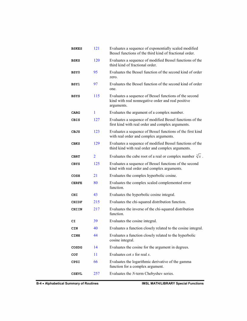
B-4 � Alphabetical Summary of Routines IMSL MATH/LIBRARY Special Functions
BSKES 121 Evaluates a sequence of exponentially scaled modified Bessel functions of the third kind of fractional order.
BSKS 120 Evaluates a sequence of modified Bessel functions of the third kind of fractional order.
BSY0 95 Evaluates the Bessel function of the second kind of order zero.
BSY1 97 Evaluates the Bessel function of the second kind of order one.
BSYS 115 Evaluates a sequence of Bessel functions of the second kind with real nonnegative order and real positive arguments.
CARG 1 Evaluates the argument of a complex number.
CBIS 127 Evaluates a sequence of modified Bessel functions of the first kind with real order and complex arguments.
CBJS 123 Evaluates a sequence of Bessel functions of the first kind with real order and complex arguments.
CBKS 129 Evaluates a sequence of modified Bessel functions of the third kind with real order and complex arguments.
CBRT 2 Evaluates the cube root of a real or complex number 3 x .
CBYS 125 Evaluates a sequence of Bessel functions of the second kind with real order and complex arguments.
COSH 21 Evaluates the complex hyperbolic cosine.
CERFE 80 Evaluates the complex scaled complemented error function.
CHI 43 Evaluates the hyperbolic cosine integral.
CHIDF 215 Evaluates the chi-squared distribution function.
CHIIN 217 Evaluates the inverse of the chi-squared distribution function.
CI 39 Evaluates the cosine integral.
CIN 40 Evaluates a function closely related to the cosine integral.
CINH 44 Evaluates a function closely related to the hyperbolic cosine integral.
COSDG 14 Evaluates the cosine for the argument in degrees.
COT 11 Evaluates cot x for real x.
CPSI 66 Evaluates the logarithmic derivative of the gamma function for a complex argument.
CSEVL 257 Evaluates the N-term Chebyshev series.
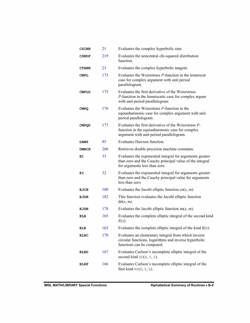
IMSL MATH/LIBRARY Special Functions Alphabetical Summary of Routines � B-5
CSINH 21 Evaluates the complex hyperbolic sine.
CSNDF 219 Evaluates the noncentral chi-squared distribution function.
CTANH 23 Evaluates the complex hyperbolic tangent.
CWPL 173 Evaluates the Weierstrass P-function in the lemniscat case for complex argument with unit period parallelogram.
CWPLD 175 Evaluates the first derivative of the Weierstrass P-function in the lemniscatic case for complex argum with unit period parallelogram.
CWPQ 176 Evaluates the Weierstrass P-function in the equianharmonic case for complex argument with unit period parallelogram.
CWPQD 177 Evaluates the first derivative of the Weierstrass P-function in the equianharmonic case for complex argument with unit period parallelogram.
DAWS 85 Evaluates Dawson function.
DMACH 266 Retrieves double precision machine constants.
E1 33 Evaluates the exponential integral for arguments greater than zero and the Cauchy principal value of the integral for arguments less than zero.
EI 32 Evaluates the exponential integral for arguments greater than zero and the Cauchy principal value for arguments less than zero.
EJCN 180 Evaluates the Jacobi elliptic function cn(x, m).
EJDN 182 This function evaluates the Jacobi elliptic function dn(x, m).
EJSN 178 Evaluates the Jacobi elliptic function sn(x, m).
ELE 165 Evaluates the complete elliptic integral of the second kind E(x).
ELK 163 Evaluates the complete elliptic integral of the kind K(x).
ELRC 170 Evaluates an elementary integral from which inverse circular functions, logarithms and inverse hyperbolic functions can be computed.
ELRD 167 Evaluates Carlson�s incomplete elliptic integral of the second kind RD(X, Y, Z).
ELRF 166 Evaluates Carlson�s incomplete elliptic integral of the first kind RF(X, Y, Z).

B-6 � Alphabetical Summary of Routines IMSL MATH/LIBRARY Special Functions
ELRJ 169 Evaluates Carlson�s incomplete elliptic integral of the third kind RJ(X, Y, Z, RHO).
ENE 35 Evaluates the exponential integral of integer order for arguments greater than zero scaled by EXP(X).
ERF 76 Evaluates the error function.
ERFC 77 Evaluates the complementary error function.
ERFCE 79 Evaluates the exponentially scaled complementary error function.
ERFCI 83 Evaluates the inverse complementary error function.
ERFI 82 Evaluates the inverse error function.
ERSET 261 Set error handler default print and stop actions.
EXPRL 4 Evaluates (ex � 1)/x for real or complex x.
FAC 48 Evaluates the factorial of the argument.
FDF 222 Evaluates the F distribution function.
FIN 223 Evaluates the inverse of the F distribution function.
FRESC 86 Evaluates the cosine Fresnel integral.
FRESS 88 Evaluates the sine Fresnel integral.
GAMDF 225 Evaluates the gamma distribution function.
GAMI 59 Evaluates the incomplete gamma function.
GAMIC 61 Evaluates the complementary incomplete gamma function.
GAMIT 63 Evaluates the Tricomi form of the incomplete gamma function.
GAMMA 51 Evaluates the real or complex gamma function, (x).
GAMR 54 Evaluates the reciprocal of the real or complex gamma function, 1/(x).
GCDF 233 Evaluates a general continuous cumulative distribution function given ordinates of the density.
GCIN 236 Evaluates the inverse of a general continuous cumulative distribution function given ordinates of the density.
HYPDF 194 Evaluates the hypergeometric distribution function.
HYPPR 196 Evaluates the hypergeometric probability function.
IERCD 262 Retrieves the integer code for an informational error.
IFNAN 266 Checks if a value is NaN (not a number).
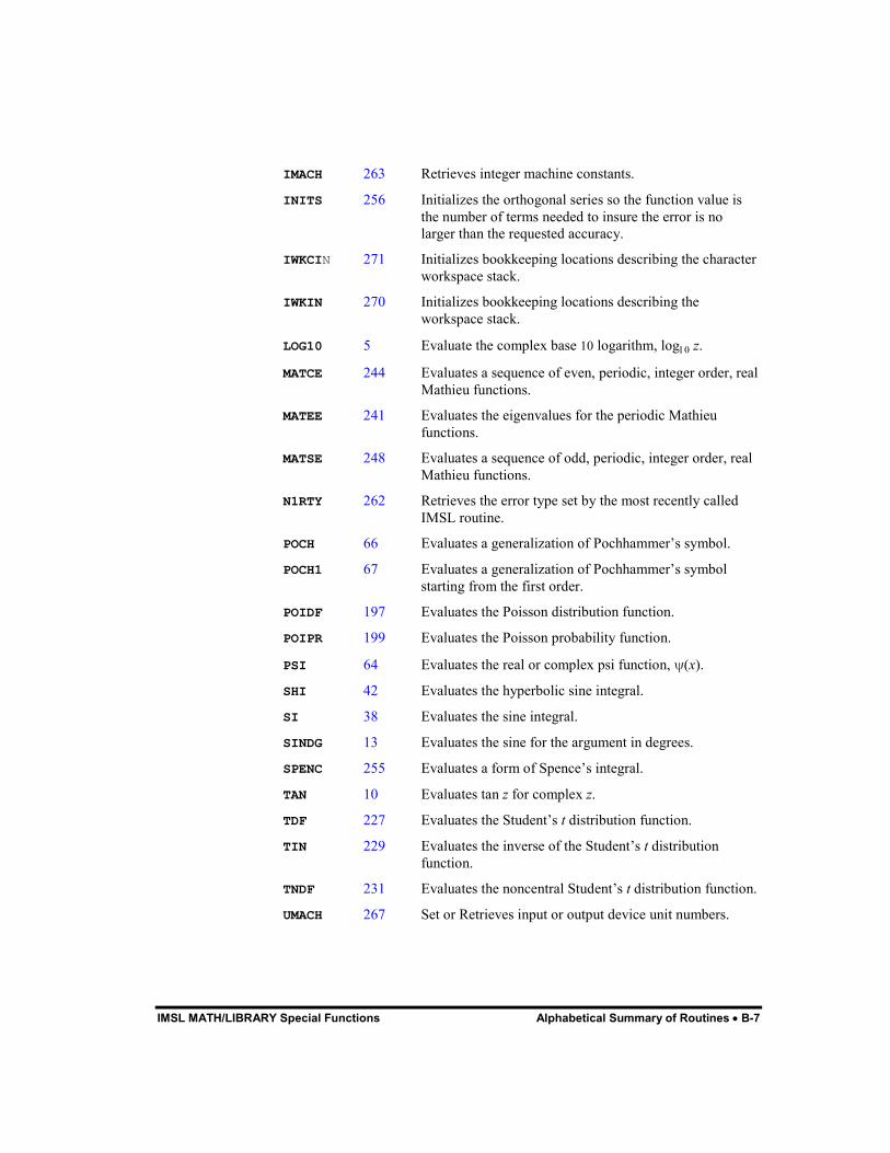
IMSL MATH/LIBRARY Special Functions Alphabetical Summary of Routines � B-7
IMACH 263 Retrieves integer machine constants.
INITS 256 Initializes the orthogonal series so the function value is the number of terms needed to insure the error is no larger than the requested accuracy.
IWKCIN 271 Initializes bookkeeping locations describing the character workspace stack.
IWKIN 270 Initializes bookkeeping locations describing the workspace stack.
LOG10 5 Evaluate the complex base 10 logarithm, log�� z.
MATCE 244 Evaluates a sequence of even, periodic, integer order, real Mathieu functions.
MATEE 241 Evaluates the eigenvalues for the periodic Mathieu functions.
MATSE 248 Evaluates a sequence of odd, periodic, integer order, real Mathieu functions.
N1RTY 262 Retrieves the error type set by the most recently called IMSL routine.
POCH 66 Evaluates a generalization of Pochhammer�s symbol.
POCH1 67 Evaluates a generalization of Pochhammer�s symbol starting from the first order.
POIDF 197 Evaluates the Poisson distribution function.
POIPR 199 Evaluates the Poisson probability function.
PSI 64 Evaluates the real or complex psi function, �(x).
SHI 42 Evaluates the hyperbolic sine integral.
SI 38 Evaluates the sine integral.
SINDG 13 Evaluates the sine for the argument in degrees.
SPENC 255 Evaluates a form of Spence�s integral.
TAN 10 Evaluates tan z for complex z.
TDF 227 Evaluates the Student�s t distribution function.
TIN 229 Evaluates the inverse of the Student�s t distribution function.
TNDF 231 Evaluates the noncentral Student�s t distribution function.
UMACH 267 Set or Retrieves input or output device unit numbers.

B-8 � Alphabetical Summary of Routines IMSL MATH/LIBRARY Special Functions

IMSL MATH/LIBRARY Special Functions Appendix C: References � C-1
Appendix C: References
Abramowitz and Stegun Abramowitz, Milton, and Irene A. Stegun (editors) (1964), Handbook of Mathematical Functions with Formulas, Graphs, and Mathematical Tables, National Bureau of Standards, Washington.
Aird and Howell Aird, Thomas J., and Byron W. Howell (1991), IMSL Technical Report 9103, IMSL, Houston.
Akima Akima, H. (1970), A new method of interpolation and smooth curve fitting based on local procedures, Journal of the ACM, 17, 589�602.
Barnett Barnett, A.R. (1981), An algorithm for regular and irregular Coulomb and Bessel functions of real order to machine accuracy, Computer Physics Communication, 21, 297�314.
Boisvert, Howe, Kahaner, and Springmann Boisvert, Ronald F., Sally E. Howe, David K. Kahaner, and Jeanne L. Springmann (1990), Guide to Available Mathematical Software, NISTIR 90-4237, National Institute of Standards and Technology, Gaithersburg, Maryland.
Boisvert, Ronald F., Sally E. Howe, and David K. Kahaner (1985), GAMS: A framework for the management of scientific software, ACM Transactions on Mathematical Software, 11, 313�355.
Bosten and Battiste Bosten, Nancy E., and E.L. Battiste (1974b), Incomplete beta ratio, Communications of the ACM, 17, 156�157.
Bosten, Nancy E., and E.L. Battiste (1974), Remark on algorithm 179, Communications of the ACM, 17, 153.
Burgoyne Burgoyne, F.D. (1963), Approximations to Kelvin functions, Mathematics of Computation 83, 295�298.
C-2 � Appendix C: References IMSL MATH/LIBRARY Special Functions
Carlson Carlson, B.C. (1979), Computing elliptic integrals by duplication, Numerische Mathematik, 33, 1�16.
Carlson and Notis Carlson, B.C., and E.M. Notis (1981), Algorithms for incomplete elliptic integrals, ACM Transactions on Mathematical Software, 7, 398�403.
Cody Cody, W.J. (1969) Performance testing of function subroutines, Proceedings of the Spring Joint Computer Conference, American Federation for Information Processing Societies Press, Montvale, New Jersey, 759�763.
Cody, W.J. (1983), Algorithm 597: A sequence of modified Bessel functions of the first kind, ACM Transactions on Mathematical Software, 9, 242�245.
Cody et al. Cody, W.J., R.M. Motley, and L.W. Fullerton (1976), The computation of real fractional order Bessel functions of the second kind, Applied Mathematics Division Technical Memorandum No. 291, Argonne National Laboratory, Argonne.
Conover Conover, W.J. (1980), Practical Nonparametric Statistics, 2d ed., John Wiley & Sons, New York.
Cooper Cooper, B.E. (1968), Algorithm AS4, An auxiliary function for distribution integrals, Applied Statistics, 17, 190�192.
Eckhardt Eckhardt, Ulrich (1977), A rational approximation to Weierstrass� P-function. II: The Lemniscatic case, Computing, 18, 341�349.
Eckhardt, Ulrich (1980), Algorithm 549: Weierstrass� elliptic functions, ACM Transactions on Mathematical Software, 6, 112�120.
Fox et al. Fox, P.A., A.D. Hall, and N.L. Schryer (1978), The PORT mathematical subroutine library, ACM Transactions on Mathematical Software, 4, 104�126.
Gautschi Gautschi, Walter (1964), Bessel functions of the first kind, Communications of the ACM, 7, 187�198.
IMSL MATH/LIBRARY Special Functions Appendix C: References � C-3
Gautschi, Walter (1969), Complex error function, Communications of the ACM, 12, 635. Gautschi, Walter (1970), Efficient computation of the complex error function, SIAM Journal on Mathematical Analysis, 7, 187�198.
Gautschi, Walter (1974), Algorithm 471: Exponential integrals, Collected Algorithms from CACM, 471.
Gautschi, Walter (1979), A computational procedure for the incomplete gamma function, ACM Transactions on Mathematical Software, 5, 466�481.
Gautschi, Walter (1979), Algorithm 542: Incomplete gamma functions, ACM Transactions on Mathematical Software, 5, 482�489.
Gradshteyn and Ryzhik Gradshteyn, I.S. and I.M. Ryzhik (1965), Table of Integrals, Series, and Products, (translated by Scripta Technica, Inc.), Academic Press, New York.
Hart et al. Hart, John F., E.W. Cheney, Charles L. Lawson, Hans J. Maehly, Charles K. Mesztenyi, John R. Rice, Henry G. Thacher, Jr., and Christoph Witzgall (1968), Computer Approximations, John Wiley & Sons, New York.
Hill Hill, G.W. (1970), Student�s t-distribution, Communications of the ACM, 13, 617�619.
Hodge Hodge, D.B. (1972), The calculation of the eigenvalues and eigenvectors of Mathieu�s equation, NASA Contractor Report, The Ohio State University, Columbus, Ohio.

C-4 � Appendix C: References IMSL MATH/LIBRARY Special Functions
IEEE ANSI/IEEE Std 754-1985 (1985), IEEE Standard for Binary Floating-Point Arithmetic, The IEEE, Inc., New York.
Johnson and Kotz Johnson, Norman L., and Samuel Kotz (1969), Discrete Distributions, Houghton Mifflin Company, Boston.
Johnson, Norman L., and Samuel Kotz (1970a), Continuous Distributions-1, John Wiley & Sons, New York.
Johnson, Norman L., and Samuel Kotz (1970b), Continuous Distributions-2, John Wiley & Sons, New York.
Kendall and Stuart Kendall, Maurice G., and Alan Stuart (1979), The Advanced Theory of Statistics, Volume 2: Inference and Relationship, 4th ed., Oxford University Press, New York.
Kim and Jennrich Kim, P.J., and Jennrich, R.I. (1973), Tables of the exact sampling distribution of the two sample Kolmogorov-Smirnov criterion Dmn (m < n), in Selected Tables in Mathematical Statistics, Volume 1, (edited by H.L. Harter and D.B. Owen), American Mathematical Society, Providence, Rhode Island.
Kinnucan and Kuki Kinnucan, P., and H. Kuki (1968), A single precision inverse error function subroutine, Computation Center, University of Chicago.
Luke Luke, Y.L. (1969), The Special Function and their Approximations, Volume 1, Academic Press, 34.
NATS FUNPACK NATS (National Activity to Test Software) FUNPACK (1976), Argonne National Laboratory, Argonne Code Center, Argonne.
Olver and Sookne Olver, F.W.J., and D.J. Sookne (1972), A note on the backward recurrence algorithms, Mathematics of Computation, 26, 941�947.
Owen Owen, D.B. (1962), Handbook of Statistical Tables, Addison-Wesley Publishing Company, Reading, Mass.

IMSL MATH/LIBRARY Special Functions Appendix C: References � C-5
Owen, D.B. (1965), A special case of the bivariate non-central t-distribution, Biometrika, 52, 437�446.
Pennisi Pennisi, L.L. (1963), Elements of Complex Variables, Holt, Rinehart and Winston, New York.
Skovgaard Skovgaard, Ove (1975), Remark on algorithm 236, ACM Transactions on Mathematical Software, 1, 282�284.
Sookne Sookne, D.J. (1973a), Bessel functions I and J of complex argument and integer order, National Bureau of Standards Journal of Research B, 77B, 111�114.
Sookne, D.J. (1973b), Bessel functions of real argument and integer order, National Bureau of Standards Journal of Research B, 77A, 125�132.
Strecok Strecok, Anthony J. (1968), On the calculation of the inverse of the error function, Mathematics of Computation, 22, 144�158.
Temme Temme, N. M. (1975), On the numerical evaluation of the modified Bessel function of the third kind, Journal of Computational Physics, 19, 324�337.
Thompson and Barnett Thompson, I.J. and A.R. Barnett (1987), Modified Bessel functions I�(z) and K�(z) of real order and complex argument, to selected accuracy, Computer Physics Communication, 47, 245�257.

C-6 � Appendix C: References IMSL MATH/LIBRARY Special Functions

IMSL MATH/LIBRARY Special Functions Product Support � i
Product Support
Contacting Visual Numerics Support Users within support warranty may contact Visual Numerics regarding the use of the IMSL Libraries. Visual Numerics can consult on the following topics:
Clarity of documentation
Possible Visual Numerics-related programming problems
Choice of IMSL Libraries functions or procedures for a particular problem
Evolution of the IMSL Libraries
Not included in these consultation topics are mathematical/statistical consulting and debugging of your program.
Consultation Contact Visual Numerics Product Support by faxing 713/781-9260 or by emailing:
The following describes the procedure for consultation with Visual Numerics.
1. Include your serial (or license) number
2. Include the product name and version number: IMSL Fortran Library Version 5.0
3. Include compiler and operating system version numbers
4. Include the name of the routine for which assistance is needed and a description of the problem
IMSL MATH/LIBRARY Special Functions Index � iii
Index
A
adjoint matrix x Airy function 149
derivative 152 exponentially scaled 154
derivative 157 second kind 150
derivative 153 exponentially scaled 155 exponentially scaled derivative
158 arguments, optional subprogram
xii
B
Bessel functions 91 first kind
integer order 109, 4 order one 94 order zero 92 real order 113, 123
modified exponentially scaled 104, 106,
107, 108, 118, 121 first kind, integer order 111, 5, 3 first kind, nonnegative real order
118 first kind, order one 100, 106 first kind, order zero 98, 104 first kind, real order 117, 127 second kind, real order 129 third kind, fractional order 120,
121 third kind, order one 103, 108 third kind, order zero 101, 107
second kind order one 97 order zero 95 real nonnegative order 115 real order 125
beta functions complete 51, 69
natural logarithm 71 incomplete 73
binomial coefficient 50
C
Cauchy principal value 32, 33 character workspace 271 characteristic values 241 Chebyshev series 253, 257 complex numbers
evaluating 1 cosine
arc hyperbolic 25
complex 17 hyperbolic 21
in degrees 14 integrals 39, 40
hyperbolic 43, 44 cotangent
evaluating 11 cube roots
evaluating 2 cumulative distribution functions
(CDF) 186
D
Dawson�s function evaluating 85
Dawson's function 75 distribution functions 186
beta 209 inverse 212
binomial 190 bivariate normal 213 chi-squared 215
inverse 217 noncentral 219
cumulative (CDF) 186 F 222
inverse 223 gamma 225 general continuous cumulative 233
inverse 236 hypergeometric 194 Kolmogorov-Smirnov goodness of
fit 204 Poisson 197 standard normal (Gaussian) 206
inverse 208
iv � Index IMSL MATH/LIBRARY Special Functions
Student's t 227 noncentral 231
DOUBLE PRECISION types ix
E
eigenvalues 241 elementary functions viii, 1 elliptic functions 173 elliptic integrals 161
complete 163 second kind 165
first kind Carlson's incomplete 166
second kind Carlson's incomplete 167
third kind Carlson's incomplete 169
Erlang distribution 226 error functions 75, 76
complementary 77 complex scaled 80 exponentially scaled 79 inverse 83
inverse 82 error handling 262 error-handling xi, xiii errors 259, 261
alert 190, 260 fatal 260 informational 259 note 190, 260 severity level xii terminal 190, 259, 260 warning 190, 260
exponential functions first order 4
exponential integrals 31, 32, 33 of integer order 35
F
factorial 48 Fresnal integrals 75
cosine 86 sine 88
G
gamma distributions standard 186
gamma functions 47 complete 51 incomplete 59
complementary 61 Tricomi form 63
logarithmic derivative 64 reciprocal 54
getting started xii
H
hyperbolic functions viii, 9
I INTEGER types ix
J
Jacobi elliptic function 178, 180, 182, 6, 5
K
Kelvin function first kind
order one 145 order zero 135, 136, 139, 140
second kind order one 146, 147 order zero 137, 138, 141, 142
Kolmogorov-Smirnov goodness of fit D-test statistic 204
L
library subprograms x logarithmic integrals 36 logarithms
complex common 5
for gamma functions 55, 57 natural 6, 71
M
machine-dependent constants 263 Mathieu functions 241
even 244 integer order 244, 248 odd 248 periodic 241, 244, 248 real 244, 248
matrices adjoint x orthogonal x
IMSL MATH/LIBRARY Special Functions Index � v
unitary x
N
naming conventions ix NaN 190
O
optional argument xii optional data xii optional subprogram arguments
xii orthogonal
matrix x orthogonal series 256
P
Pochhammer's symbol 66, 67, 253 printing 261 printing results xiii probability density function (PDF)
187 probability distribution functions 185
inverses 185 probability functions 186
binomial 191 hypergeometric 196 Poisson 199
R
REAL types ix required arguments xii reserved names 269
S
sine arc
hyperbolic 24 complex
arc 16 hyperbolic 20
in degrees 13 integrals 38
hyperbolic 42 single precision vii Spence's integral 255 subprograms
library x optional arguments xii
T
tangent arc
hyperbolic 27 complex 10
arc 18 arc of a ratio 19 hyperbolic 23
Taylor series 253 trigonometric functions viii, 9
U
underflow x unitary matrix x user interface vii using library subprograms x
W
Weierstrass' function equianharmonic case 176, 177 lemniscatic case 173, 175
workspace allocation 270

vi � Index IMSL MATH/LIBRARY Special Functions