Research Collection

Doctoral Thesis

Numerical methods for the inversion of Laplace transforms

Author(s): Boutros, Youssef Zaki

Publication Date: 1964

Permanent Link: https://doi.org/10.3929/ethz-a-000087892

Rights / License: In Copyright - Non-Commercial Use Permitted

This page was generated automatically upon download from the ETH Zurich Research Collection. For moreinformation please consult the Terms of use.

ETH Library

Prom. Nr. 3491

NUMERICAL METHODS FOR THE INVERSION

OF LAPLACE TRANSFORMS

Thesis presented to

THE SWISS FEDERAL INSTITUTE OF TECHNOLOGY, ZURICH

for the degree of

DOCTOR OF MATHEMATICS

by

YOUSSEF ZAKI BOUTROS

B. Sc. Elec. Eng. University of Alexandria

Dipl. Math. ETH Zurich

Citizen of the United Arab Republic

Accepted on the recommendation of

Prof. Dr. E. Stiefel

Prof. Dr. P. Profos

1964

ASCHMANN & SCHELLER AG, ZURICH

Leer - Vide - Empty

Preface

The present work deals with some practical methods for the numerical in¬

version of Laplace transforms covering those which are frequently met with

in stable networks and regulation problems.

I take this opportunity to acknowledge my indebtedness and gratitude to

Prof. Dr. E. Stiefel for his generous support during the investigations for this

thesis. I wish also to express my sincere thanks to Dipl. Ing. A. Schai for the

suggestion of the practical problem of Chapter IV.

I am very grateful to Prof. Dr. P. Profos for accepting this thesis.

YoussefZ. Boutros

Zurich, December 1963.

3

Leer - Vide - Empty

Index

Page

Chapter I: Introduction 7

Chapter II: Inversion of Laplace Transforms using Laguerre Functions 8-25

1. Development of the method 8

2. Procedure for the practical application 12

3. Remarks 13

4. Numerical examples 21

5. Conclusion 25

Chapter III: Laplace Transforms with known Position of the Dominant Pole 25-35

1. Simple real pole 25

2. Conjugate complex pair of poles 28

3. Remarks 35

Chapter IV: Position Control System with Load Disturbance 35-52

1. Determination of C/R 37

2. Determination of C/TL 40

3. Output c (t) corresponding to different inputs on both sides 42

Chapter V: Linear Flow of Heat 52-60

1. Development of the method 52

2. Numerical examples 58

Appendix 61

References 63

Zusammenfassung 64

Curriculum vitae 64

5

Leer - Vide - Empty

CHAPTER I

Introduction

The present work deals with the problem of determining the inverse function

of a given Laplace transform, which is assumed to be analytic in the entire

right half plane including the imaginary axis. This method of determining the

inverse function requires only the numerical values of the transform at these

points which are distributed on the imaginary axis in a given way, or even on

an axis parallel to it and lying entirely in the domain of regularity of the giventransform. In case of an empirically given function, it is more convenient to

calculate the values of the transform directly at these given points (otherwise

by interpolation in these points). However, the inverse function will be deter¬

mined as a finite sum of Laguerre functions, which represents it over every

finite time interval 0^t1-^tSU<co-

Laplace transforms which satisfy the formerly stated conditions are fre¬

quently met with in the analysis of stable networks of electrical engineeringand in regulation problems. Here the singularities of the transfer function are

mainly poles which lie to the left of the imaginary axis. Because it is difficult

in general to find an explicit expression for the transfer function, it is usually

measured experimentally at various frequencies (these can be chosen directly,

and are those mentioned above).In Chapter II, the general method of inversion is developed, while in the

remarks other types of transforms, not satisfying exactly the above require¬

ments, are treated. Besides, the convergence of the Laguerre series is fully

discussed. It is proved that this method delivers, for t = 0, the actual value f (0)1

of the original function and not its mean value — f (0) as in the case of Fourier

inversion.

Chapter III treats the case where the position, and only the position, of the

dominant pole*) of the transform is known. Thus, we are able to obtain the

asymptotical behaviour of the inverse function as well. Numerical examples

are given at the end of each chapter.

In Chapter IV, a practical problem concerning a position control system is

completely solved. The results are found to be very satisfactory and confirm

the stability of this method.

Chapter V deals with the application of the method of Chapter II to the

problem of the linear flow of heat.

The appendix contains the program necessary for the practical use of this

method on computers. It is written in the Algol language.

*) The pole having the largest real part.

7

CHAPTER II

Inversion of the Laplace Transforms using Laguerre Functions

/. Development of the method

00

The Laplace transform F (p) = J f (t)e_ptdt, considered as a functiono

of the complex variable p = s + i co, is assumed to be analytic in the right half

plane including the imaginary axis. Further, let lim {pF (p)}, p = io>, exist

and be finite and uniquely determined as p approaches infinity in both direc¬

tions of the imaginary axis*). Besides, assume F (p) can be calculated numer¬

ically at arbitrary points of the imaginary axis. This is almost always the case

in stable networks, where the frequency response is known.

The main idea of this method of inversion consists in finding a suitable

representation of the given transform in its domain of regularity, using a

certain class of functions whose inversion is known. For this purpose, we make

use of the conformal mapping

/ —P(1)

l + P

of the complex plane on itself; / is a real positive number (see II.3, Remark 3).This transformation maps the entire right half plane into the interior of the

unit circle. The unit circle itself becomes the image of the infinite imaginary axis.

Let us now introduce the function

G (p) = (/ + p) F (p). (2)

It remains finite even as p tends to ± i oo. The reason why we multiply F (p)

by (I + P) will be explained later. Further, we express G (p) in terms of the

new variable z and denote the resulting function by G (z). This function is

finite on the unit circle and analytic in its interior. We approximate G (z) by

a polynomial

P (z) =n^Ck zk (3)k = 0

and calculate its coefficients Ck by interpolation to the function G (z) in

*) For the refinement of the method we shall assume sometimes F (p) to be regular at

infinity.

n points on the unit circle*). We divide the unit circle in n equal parts and

numerate the points of division in a clockwise sense beginning from the pointz = 1 (the image of p = 0). Moreover, let us denote the n-th root of unity by

w = e_i9,

2tcwhere & =

. It should be noted that wn = 1 or

n

wn—1 = (w—1)(1 + w + w2+ ... + w"-1) = 0,

n—1

that is, J] wk = 0 for a root of unity w ^ 1. In generalk = 0

n—1

£ Wmk = 0, wm # 1,k = 0

for wm is also a root of unity. In other words

"yV*=

( n f°r m = °' n' 2n' -'(4)

k^0 \ 0 otherwise. l '

The points of division on the unit circle will be

zv = wv = e-iva,v = 0, 1,2, ...,(n-l).

The inverse images of these points lie on the imaginary axis of the p plane,symmetrically with respect to the origin, and are given by

icov = U tan (v&/2), v = 0, 1, ..., (n— 1).

Let now P (z) interpolate G (z) in the points zv.

P (zv) = G (zv) = G (i«v) = (/ + i<> F (icov), v = 0, 1, ..., (n - 1).

This yields the following system of linear equations for the determination of the

polynomial coefficients Ck:

n^Cm wvm = (/ + i<> F (icov), v = 0, 1, ..., (n - 1).m = 0

*) Harmonic analysis. However, if n —> oo the polynomial (3) becomes the Taylor ex¬

pansion of G (z) at the point z = 0 and the coefficients C^ become its Fourier coefficients.

This series converges everywhere in the interior of the unit circle.

9

10

57):85,p.result:8;75,p.40;78,p.3;75,p.3;81,p.

[4]:(seefollowsasstepsinoutcarriedbewilltransformthisofinversionThe

1+q)k+(2/I+p)k+(/

(-l)kqk(/-p)k

—/.p=q

variablenewtheintroduce

weplacefirsttheIninverted.becouldfunctionsrationalresultingthethat

soonebynumeratortheofthatexceedsdenominatortheofdegreetheway

thisIn(2).inp)+(/by(p)Fmultipliedhavewewhyobviousisitplacethis

Atdetermined.beeasilycaninversionwhosetransformsLaplacesimpleare

P)k+(/...,(n-l),1,0,=k1^-,

-^ —p)k(/

functionsThe

(/+p)K+1o=kp/+\/o=(/+p)kp)+(/(6)•

ot+i,,,^L=

in—1ck£~=(p)f

and

0=k

G(z)~£Ckz<,k

n—1

namely(p),Fand(z)GforrepresentationsfollowingthehaveweThus,

defined.completelyis(z)Gof(z)PpolynomialapproximatingtheNow,

v=0n

(5)1).-(n...,1,0,=kw"vk,(itov)Fi«v)+(/£-=Ck

nCk.is

thatandk,=mforonly05^valueahassideright-handthe(4)toAccording

wvc°-k>.2cm£=cmwv(—«££

=w-vk(icv)Fi<>+(/£v=0m=0v=Om=0

£cmw^-«=£cm2>£

=

n—1n—11—nn—1

1).—(nto0from

voversumandvkwbysidesbothonmultiplywesystemthissolvetoorderIn

Laplace transform Inverse function

1e"2/t

(2/+q)

1 tk

(2/ + q)k+1 k!e"2/t

qk 1 dkq(tke"2/t)

(2/ + q)k+1 k! dtk

(/ + p)k + 1 k! dtk

The last inverse function can be expressed in terms of the Laguerre functions.

These are defined as (see [6])

et/2 dk.

t

They build an orthogonal system of damped functions in the interval (0, oo)

and have all the value 1 at t = 0.

Hence we can write the last inverse function of the table above as

(-l)k/k(2/t).

Inverting F (p) in (6) term by term we obtain its inverse function f (t)

f(t)~n£1(-l)k 0^(2/1). (7)k = 0

Since /k (t) takes on real values for real arguments t, so should f (t). Therefore,

in (7) we shall need only the real parts of the coefficients C^. If we write

Ck = £k + i%»

f (t) reduces to

f(t)~nS1(-l)Hk/k(2/t). (8)

11

On the other hand, let

(/ + iwv) F (iwv) = av + i(3v.

Substituting this in the expression (5) for Ck we get for the real part

1 "-1/ 2tt 2n\

lk = — >, lavcosvk pvsinvk . (9)n

v = o \ n n '

In almost all practical cases and especially in electrical networks, the trans¬

form F (p) takes on real values for real arguments. Moreover, the points of

division on the unit circle zv and zn_v are conjugate complex. Hence, accord¬

ing to the Schwarz principle of reflection, the values (/+ icov)F(iwv) and

(/ + io>n_v) F(ia)n_v) in the sum (5) will be conjugate complex. Thus, the

coefficients Ck will be all real. That is, the imaginary parts 7)k are not present

at all.

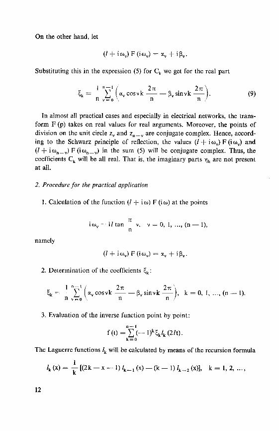
2. Procedure for the practical application

1. Calculation of the function (/ + i to) F (i oj) at the points

icov = i/ tan -

v, v = 0, 1, ..., (n — 1),n

namely

(/ + itov) F (icov) = ocv + ipv.

2. Determination of the coefficients \y:

1 n-'/ 7-k 2n\

Kk = — L «v cosvk (3V sinvk ,k = 0, 1, ..., (n — 1).

nv = o \ n n /

3. Evaluation of the inverse function point by point:

f(t)=n£(-l)ki;k/k(2/t).k = 0

The Laguerre functions lk will be calculated by means of the recursion formula

k W =

yK2k - x - l) 4-i W - (k - l) /k_2 (x)], k = l, 2, ...,

12

where /_, (x) = 0 and l0 (x) = e~x/2.

3. Remarks

1. This method of inversion can be modified somewhat to suit the case where

the transform F (p) is given on an axis parallel to the imaginary axis and which

lies entirely in the domain of regularity of F (p). Let this axis have the equation

p = a, where a > 0. The parallel translation q = p — a reduces this case to

the previous one. Hence, we invert F (q) as before and then multiply the result

by the factor eat to obtain the inverse of F (p). This parallel translation can be

used in order to avoid any finite singularities of F (p) which may lie on the

imaginary axis of the transform plane. In this case the value of F (p) on this

new axis will be needed.

2. Let p = oo be an essentially singular point of F (p); the value F (i oo) will

be required in calculating (/ + iwv) F (i^v) f°r v — n/2- The point p = oo

corresponds to the point z = — 1 by means of the conformal mapping

/+P

Hence, if G (z = — 1) can not be easily calculated, then we make the regulardivision as stated before, not on the unit circle | z | = 1 but on a concentric

one with radius r, 0 < r < 1. Its inverse image in the transform plane is againa circle which lies entirely to the right of the imaginary axis and has its centre

on the real axis. On this circle the function (/ + p) F (p) is completely defined.

The points of division in the z plane are in this case

zv = rwv

where w = e—l2"/n. The inverse images in the transform plane are

1 — zv / (1 — r2) + i2/r sin v27r/np„ = s„ + io)„ = / =

.Fv v

l + zv (1 + r2) + 2rcosv27r/n

The procedure for the determination of the coefficients £k should be modified

as follows:

13

G^-^C^k = 0

Gv = G (zv) = (/ + pv) F (pv) = a, + ipv

n—1

= £Ck(Zv)kk = 0

at\ckTk) Wvkk = 0

1 t 1

nr v=o

=—r- Y" (av + i(3v) cosvk h i sinvknr^vfo \ n n /

1 n—' / 2tc 27t

£k = 3d {Ck} = —j-V (ccv cosvk pv sinvk

nr v=0\ n n

3. Choice of /: In the following, we shall assume F (p) to be regular at infi¬

nity. The mapping parameter / affects a dilatation in the transform plane,because

l-V=

1-(P/Q

/ + p 1 + (p//)'

For every finite positive /, the right half plane will be mapped into the unit

circle and the imaginary axis will always have the unit circle as image, see

Figure II-1. According to our assumptions for F (p), the singularities of G (z)can only lie outside this circle. Now, if we let the degree of the approximating

polynomial P (z) tend to infinity, we obtain the Taylor expansion of G (z) at

the point z = 0. This series converges inside the circle with centre at the originand passing through the next singularity of G (z); accordingly, its radius is

greater than 1. Thus, the convergence of this series on the unit circle can be

accelerated by making the circle of convergence as large as possible. This can

be achieved by an appropriate choice of /. In this way, the approximation of

G (z) by a polynomial P (z) of fixed degree (n — 1) will be improved.

As said before, a circle having its centre at the origin of the z plane will have

as inverse image, a circle with centre on the real axis. Here, the circle of con-

14

\N_ N

sC t^j *** Uj

/ /\ !>

•=jf / \ wX /

u.

c

N

3

c

to

15

vergence lies to the exterior of the unit circle. Therefore, its inverse image will

lie entirely in the left half plane. Moreover, it should be noted that the point

z = oo is the image of p = — / (Figure II-1). Hence, enlarging the radius of the

circle of convergence will mean diminishing that of its original image. Accord¬

ingly, if we can guess where the singularities of F (p) may lie, even as a cloud,

then we try to enclose them inside the circle lying entirely in the left half plane,

having its centre on the negative real axis, and subtending the smallest angle

at the origin. The length of the tangent from the origin to this circle is the re¬

quired /.

The following special cases should also be stated:

i) Simple real pole — a, a > 0: In this case it is quite clear that / will be

directly equal to a. The image of this pole will lie at infinity.

ii) Two conjugate complex poles — a ± ib, a > 0:

For fixed / the radius of the circle, with centre at the origin and passing

through their images, is given by

__

\[P — (a2 + b2)]M^4WT_

[(/_a)2 + b2]'

It is maximum for / = ]/a2 + b2 and this maximum is

|b|fmax

V^+W-a'

1The original image of this circle will have its centre at (a2 + b2) and the

a

|b| ,,

radius y a2 + b2.In other words, this circle touches the radius vector of

a

each pole at this pole.

4. Choice of n: A reasonable value for n which compromises between accu¬

racy and calculation time, is found to be 24. This time is mainly proportional

ton.

5. Convergence of the Laguerre series: In our discussion we shall need a

theorem concerning the term by term inversion of series representing Laplacetransforms. For this purpose, we shall state it now (see [5], p. 186, Theorem

22.1):

16

Theorem

Let a function F (p) be represented as an infinite series:

F(p) = £Fk(p), Fk(p) = Je-"tfk(t)dt, k = 0, 1, ...,

k = 0 0

where all these integrals exist in a common half plane 91p ^ s0. In addition,

the following should hold:

a) The integrals

CO

je-pt|fk(t)|dt = Gk(p), k = 0, 1, ...,

o

should exist in this half plane, which implies that the integrals Gk (s0) exist.

b) The series

SGk(s0)k = 0

CO

should converge so that also ^ Fk (p) converges in 91p ^ s0 absolutely and

k = 0

uniformly.

CO

Then ^ fk (t) converges, even absolutely, towards a function f (t) for

k = 0

almost all t 2: 0, and f (t) is the original function of F (p), i. e.

GO CO

£Fk(p) «- £fk(t).k=0 k=0

The Laplace transform of f (t) converges for 91p ^ s0 absolutely.

In addition to the former assumptions for F (p), we shall suppose it to be

analytic also at p = oo. As said before, if we let the degree n of P (z), the

approximating polynomial of G (z), tend to infinity, P (z) will be identical

with the Taylor expansion of G (z) at z = 0:

CO

G(z) = £Ckzk (10)k=0

or, in terms of p,

17

£l fl— pxk

k = o \ / + p

If we use the relation (2) connecting G (p) with F (p), we get the following

representation for F (p):

« (/ — p)k

Before we apply the theorem above, we verify at first the assumptions stated

there:

Fk (P) = Ck (jl~f,r - fk (0 = (- Dk Ck/k (2/t).

All transforms Fk (p) exist in the half plane 9tp ^ s0 > 0.

a) Since |/k (x)| ^ 1 for x k 0, the following estimation holds:

T T T

Ye—* |fk (t)| dt = /"e—' |Ck/k| dt £ |CJ / e—'dt = ~[1 - e—^

o o

Hence,

T

Gk (s0) = lim / e-sot |fk (t)| dt g lim -L^i-[1 — e-s'T] = -i^-

< oo.

T—><aj T—>oo s0 s00

1 °°

b) Since the series (10) is absolutely convergent for |z| = 1, — £] ICJso k = o

is a convergent majorant of the series Y]Gk(s0). Therefore, the latter isk=o

convergent.

Hence, we can apply the former theorem and get

f(t) = £(_l)kCk/k(2/t), (11)k = o

which converges absolutely for almost all t ^ 0 towards the actual inverse

function of F (p).

18

Moreover, we shall prove that the Laguerre series (on the right-hand side

of (11)), together with all its derivatives, converges uniformly everywhere

over every finite interval 0 ^ t ^ T < oo. Let us denote by <& (t) the function

represented by the Laguerre series (11), i. e.

O (t) = g (- l)k Ck/k {lit) = £ fk (t), (12)k=0 k=0

and let f (t) be the actual original function of F (p). The last theorem states

that f (t) and <X> (t) are identical except over a set of measure zero. Since F (p)is assumed to be analytic at infinity, f (t) will be an integral function of the

exponential type (see [5], p. 191, Theorem 22.3). Because |/k(x)| ^ 1 for

x ^ 0, k = 0, 1, 2, ... (see [10], p. 159), the following estimation holds:

ifk(t)i = i(-i)k cy.a/omcj

for all t ^ 0. Besides, the Taylor expansion (10) of G (z) converges absolutelyCO

on the unit circle so that ]T | Ck | also converges. Therefore, this is a convergentk=0

majorant for (12) whose terms are independent of t. Hence, the Laguerre series

converges uniformly (even absolutely) towards O (t) over every finite interval

0 ^ t ^ T < oo. Since the Laguerre functions are continuous for t ^ 0,

O (t) will be also continuous. Thus we have two functions, O (t) and f (t),which are both continuous and which coincide with each other for t ^ 0

except over a set of measure zero. Therefore, they are identical

*(t) = f(t), t^0.

We shall prove now that the derivative of f (t), for t ^ 0, can be obtained

by differentiating its Laguerre series term-wise. For this purpose, we state at

first some properties of the Laguerre polynomials L£a) (x) (see [10], p. 96-98

and [11]):

(a) lk (x) = e-*-'2 Lfc (x), Lk (x) = Lf (x).

(b) ~ I4°> (x) = (- l)1l£_+» (x).ax

(c) e~x/21 L£° (x) I ^ (k + a), equality holds for x = 0.

The k-th term fk of the series (12) can be rewritten in the form

fk(t) = e-'t[(-DkCkLk(2/t)].

19

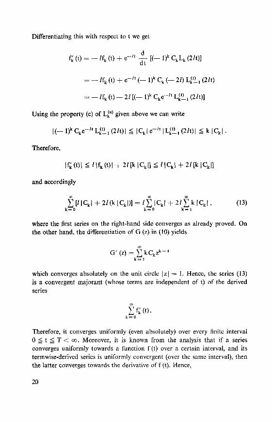
Differentiating this with respect to t we get

fk (t) = - /fk (t) + e-" — [(- l)k CkLk (2/t)]dt

= - /fk (t) + e-" (- l)k Ck (- 21) L^i, (2/t)

= - /fk (t) - 2/ [(- l)k Cke-" L*1!, (2/t)]

Using the property (c) of L^a) given above we can write

| (- l)k Cke-" U*L, (2/t) | ^ | C^| e-" | L<», (2/t) | g k | Ck | .

Therefore,

|fk(t)| g /|fk(t)| + 2/[k|Ck|] g MCJ + 2/MCkl]

and accordingly

£ [/ |Ck| + 2/(k |Ck|)] = /£|Ck| + 2#f;k|Ck|, (13)k=0 k=0 k=l

where the first series on the right-hand side converges as already proved. On

the other hand, the differentiation of G (z) in (10) yields

GO

G'(z) = £kCkzk-'k= 1

which converges absolutely on the unit circle |z| = 1. Hence, the series (13)

is a convergent majorant (whose terms are independent of t) of the derived

series

GO

k = 0

Therefore, it converges uniformly (even absolutely) over every finite interval

0^ t^T< oo. Moreover, it is known from the analysis that if a series

converges uniformly towards a function f (t) over a certain interval, and its

termwise-derived series is uniformly convergent (over the same interval), then

the latter converges towards the derivative of f (t). Hence,

20

Efk(ok = 0

converges towards f' (t). In the same way, we can prove that the higher derivat¬

ives of f (t) can be obtained from the former ones by further differentiation.

Thus we have the final result:

If F (p) is analytic at infinity, then the Laguerre series (11) converges uni¬

formly (even absolutely) over every finite interval 0 ^ t :g T < oo towards

the actual original function f (t), where F (p) is the Laplace transform of f (t).

The derviatives of f (t) can be obtained by differentiating the Laguerre series

of f (t) term-wise, which converges again uniformly (even absolutely) over the

same time interval.

This holds especially at t = 0 which is missing in the case of the Fourier

inversion.

4. Numerical examples

(See the Appendix for the program.)

1. Consider the transform

a

sin

p + 2F (p) = ,

a real,

(p + 1) sin —-

p + 2

which is regular at infinity and for which limp F (p) = a. It has simple polesp—> oo

at —1 and — I 2 ± ,k = 1, 2, ....

These accumulate at p = — 2 and

lie all on the negative real axis. The exact inverse is a monotone decreasing

function which falls from 0.3 at t = 0 to about 10-7 at t = 15 and is given by

sina.

1 " (— l)k sinak7t

f(t) = -—e-' + - £ ^ '—

sml -k k'Ti k

e-(2-^)' e-(2+^r)t

(kn — 1) (kic + 1)

The numerical inverse is compared with this function (for the parameters

21

1

/ ' \ ^^^/ / \ ^^/ ' \ —~_

I •!• J ^^

,

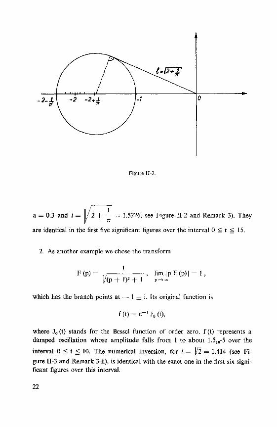
2-J.\ -2 -2+1 U 0

Figure 11-2.

a = 0.3 and / = 1/ 2 -\ = 1.5226, see Figure II-2 and Remark 3). They

are identical in the first five significant figures over the interval 0 ^ t ^ 15.

2. As another example we chose the transform

F(p)=17=L=-> lim|PF(p)| = l,]/(p + l)3 + 1 p-»»

which has the branch points at — 1 ± i. Its original function is

f(t) = e-lJ0(t),

where J0 (t) stands for the Bessel function of order zero, f (t) represents a

damped oscillation whose amplitude falls from 1 to about 1.510-5 over the

interval 0 ^ t ^ 10. The numerical inversion, for I = ]/2 = 1.414 (see Fi¬

gure II-3 and Remark 3-ii), is identical with the exact one in the first six signi¬ficant figures over this interval.

22

Figure II-3.

3. The following example is chosen to show the applicability of this method

to Laplace transforms which are not regular at infinity. Let us consider the

function

F(p)ShaVp

(p + 1) Sh 1/p,a< 1;

it has simple poles at — 1 and —k27r2 (k = 1, 2, ...) which accumulate at

infinity, lim [p F (p)] is zero as p -+ oo on all straight lines passing through the

origin, except in the direction of the negative real axis. The exact originalfunction is given by the series

f(t) =sma

sinl

£i k(— l)ksinakTC., „

2,1 V -i '- e~kn

'.

A (k27r*-l)

The transform F (p) is inverted numerically for a = 0.5 and 1=1 (in this

case / is arbitrary). Figure II-4 shows this result as well as the deviation from

the exact inverse.

23

f(t>

03.

0.2.

0.1.

Figure II-4a. The inverse function (Example 3).

Figure II-4b. The error (Example 3).

24

5. Conclusion

This method of inversion has shown its merits of being accurate, stable,

and simple in its application. It gives the inverse function, to a reasonable

degree of accuracy, at every finite t S; 0.

A similar method of inversion using Laguerre functions is developed in [8],

p. 292-303. It expands the function G (z) at the point z = 0 in a Taylor series

and determines the inverse function as a Laguerre series having mainly the

same coefficients. Numerical examples using this method have shown that

in most cases of technical significance, the computation of the coefficients of

the Taylor series from the derivatives of G (z) is, from the numerical point of

view, not feasible with sufficient accuracy. Accordingly, the Laguerre series

representing the inverse function does not converge towards the actual value

except for a very narrow time interval and with a poor degree of accuracy.

CHAPTER III

Laplace Transforms with known position of the Dominant Pole

We suppose that the position of the dominant pole of F (p) is approximately

known, while the residue in this pole can not be calculated easily. In the follow¬

ing we shall discuss two practical cases, the first concerning a simple real pole,the other a conjugate complex pair.

/. Simple real dominant pole

Let a be this pole, a < 0 real. Its image in the z plane by means of the former

conformal mapping (1) is

/ — a

a = ;/ + a

it lies again on the real axis of the z plane. We construct the function G (p) =

(/ + p) F (p) and express it in terms of the new variable z as before. Here we

interpolate the function G (z) by a rational function R (z) of the form

n—1

£ckzkR(z) = — (14)

z — a

25

which takes on the values Gv at the points zv, v = 0, 1, ..., (n — 1), namely

R (z,) = Gv = G (zv) = G (wv) = G (icov),

where wv and <ov are the same as defined in Chapter II. The coefficients Cj,are determined by means of the following system of linear equations

n—1

k = 0

_^Ckwvk = YVJ v = 0, 1, ...,(n-l),

where

Yv = (wv-a)Gv.

The solution of this system is obtained as before (see Chapter II)

Ck = -n£Yvw-v\ k = 0, 1, ...,(n-l).n

v = o

Expression (14) can be rewritten as

n— 1

L CkzkU n-2

R(Z)=J^» =_b=-l_ + SbjZi.z — a z — a j = o

Thus, we can calculate bj (j = — 1,0, 1, ...,n — 2) in terms of the C^ (k = 0,

1, ...,n — 1). This yields the following recursion formula

bj = Cj+1 + abJ + 1, j=— 1, 0, 1, ..., (n —2),

where bn_, = 0. Hence, we can write now

G (z) ~ R (z) = ~^L +n£2bkZK (15)z — a k^o

and get the following representation for the Laplace transform

F(p) = 7/-^TG(p)(f+ P)

26

l + p

b_,(/ + a) ,'n2. (/-P)"

2/(p-a) k^0ka+p)k + 1'

The inverse function of the first term is

(/ + a)

2/9t{b_,}eP

(/ —p)k .

and that of r—p is (— 1) L (2/t) as in Chapter II. Hence, the resul-(/ + p)k+I

v k F

tant inverse function of F (p) becomes

f(t)~-(/ + a)

2/

n—2

"I]k = 0

31 {b_J eat + £ (- l)k 31 {bk} lk (2/t). (16)

As in Chapter II, if F (p) takes on real values on the real axis, the coefficients

Q, and consequently the bk, will be all real. It should be noted that the above

expression for f (t) gives its actual as well as its asymptotical behaviour. Because,

if we expand F (p) around the dominant pole p = a in a Laurent series, the

principal part will have the form

p —a. The corresponding asymptotical

part of f (t) becomes

3l{A}eat.

On the other hand, the process of inversion described before will yield the

following:

F(p)p —a

+ regular part at p = a,

G(p) = (/ + p)p —a

+ regular part at p = a,

27

1—z) AG (z) = (/ + / + regular part at z == a

1 + z ) 1 —z/ a

1 + z

2/A

regular part at z = a

(/-a)-z(/ + a)

— 2/A= h regular part at z = a.

(/ + a) (z — a)

Comparing this representation of G (z) with (15) we get

— 2/Ab

,=

.-1

(/ + a)

Substituting this in the expression (16) of f (t) we obtain

2/l ~u

2/ (/ + a)

= 3i{A}eat. q.e. d.

Therefore, we have a numerical method for determining the residue A of

F (p) in the dominant pole a.

1/ 1As a numerical example we considered the first one in II.4, for / = 1/4

y it2

= 1.9745 (see Figure III-l and Remark III.3.1); the dominant pole is a = — 1.

Figure III-2 shows the inverse function as well as its asymptotical part. The

comparison between this f (t) and the exact inverse function shows that the

results are accurate to five significant figures.

2. Conjugate complex pair of dominant poles

Let us denote these poles by

^i>2 =a±ib,a <0.

28

Figure III-l.

Figure III-2. The inverse function and its asymptotical part.

29

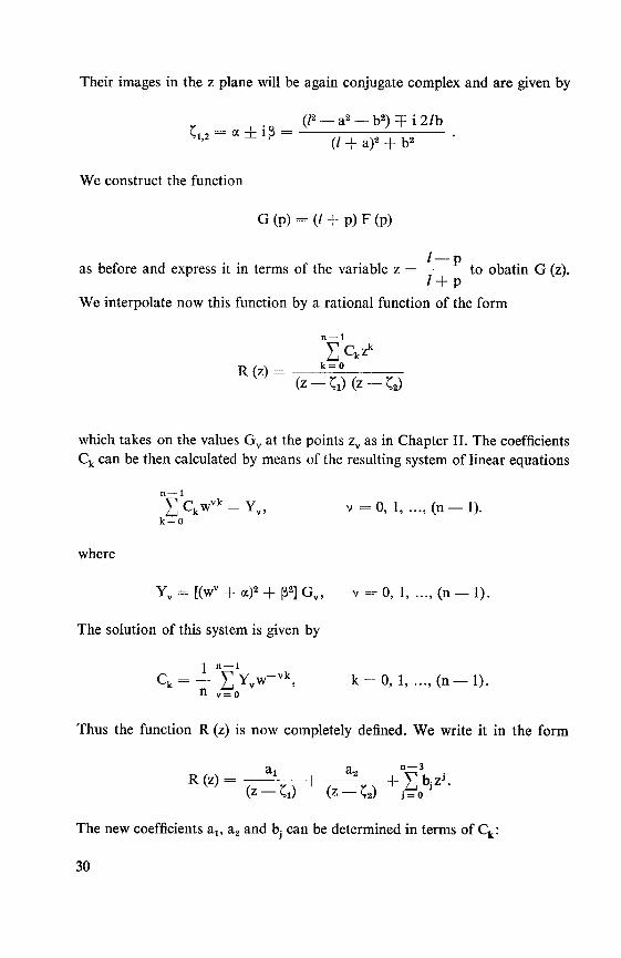
Their images in the z plane will be again conjugate complex and are given by

(/2_a2_b2)Ti2/b1,2 ^

(/ + a)2 + b2

We construct the function

G(p) = (/ + p)F(p)

/ —pas before and express it in terms of the variable z = to obatin G (z).

/ + p

We interpolate now this function by a rational function of the form

n—1

£ckzkR(z)

(z-^Mz-Q

which takes on the values Gv at the points zv as in Chapter II. The coefficients

Ck can be then calculated by means of the resulting system of linear equations

n—1

k = 0

£Ckwvk = Yv, v=0, 1, ...,(n-l).

where

Yv = [(wv + <x)2 + P2] Gv, v = 0, 1, ..., (n - 1).

The solution of this system is given by

Ck = - n^Yvw-vk, k==0, 1, ...,(n-l).n v=o

Thus the function R (z) is now completely defined. We write it in the form

ax a, n^3

The new coefficients a1; a2 and bj can be determined in terms of Ck:

30

bk = Ck + 2-(<*2+P2)bk + 2 + 2abk+1, k = 0, 1, ...,(n-3),

where bn_j = bn_2 = 0 and

k = 0

Ki— C2 2(3 k = 0

10,1*,

n—1

Eck£k=0

£2 — £i 2(3 k=o

Therefore, we write

G(z) ~R(z) = —^- +-^- + £ bk

Z — (=i Z — <,2 k=0

(17)

and

F(p)1

(/ + P)

1

(/ + P)

G(p)

/-pCi

/-pv

+k?obklTT7/ + p / + p

^2

i

Yiai (/ + Tti) a2 (/ + 7r2)

P — % P — TC2

nv3b (/~p)k

"Ak(/ + P)k+1"

The first two terms, together with the factor before the bracket, have the

inverse function

1

JR{a1(/ + 7t])e"'t + a,(/ + 7t>)e*'t}

— eat [A cos bt — B sin bt]2/

L (18)

where

31

A = (/ + a)(Tl + y2)-b(S1-S2),

B=(/+a)(81-S2) + b(Yl + y2)

(19)

and

ai = Ti + iSi,

a2 = y2 + iS2,

so that the inverse function of F (p) becomes

f (t) eat [A cos bt — B sin bt] +°£ (— l)k 9t {bk} lk (2/t).2/ k = o

This formula includes both the actual as well as the asymptotical behaviour of

the inverse function. We shall prove, in a similar way as in III.2, that the terms

before the sum give the asymptotical part of f (t). Let the principal parts

corresponding to the dominant poles be

Ax+

(A1 + A,)(p-a) + ib(A1 —A^

(p-*i) (P-O (p-a)2 + b2

The asymptotical part of f (t) is the inverse of this expression, namely

eat [91 {A1 + A2} cosbt + Sft {i (A1 — A2)} sinbt].

Inverting F (p) as before we get:

Ai A2F(p)

G(p) =

G(z)

(P — ^i) (p — rc2)+ regular part at p = iz1>2

MZ + p),

A2(/ + p)

(P — *i) (P — ^2)regular part at p = nU2

AAl + l1—z

AAl+l1—z

l+z 1+z

regular part at z = £t.

32

=

7TT—V7Z FT—

77T—V7Z FT + reSular Part at z = ^u •

(/ + Ttj) (Z — y (/ + 7r2) (Z — Q

Comparing this expression with (17) we have

— 21A1a, =

(/ + *i)

— 2/A2a, = .

Substituting this in the expression (18) for the asymptotical part we obtain

-~fft{nx(l+ tO e"" + a2 (/ + rt2) e""}

= —— 31 {— 2/Aie(a + ib)t—

2/A2e<a-ib><}

2/l ;

= eat 81 {Aieibt + A2e-ibt}

= eat [3* {A± + A2} cosbt + 31 {i (Ax — A2)} sinbt] q. e. d.

However, if the transform F (p) takes on real values on the real axis, then,

according to the discussion of Chapter II, the coefficients C^, and consequently

bk, will be all real. The coefficients a! and a2 become conjugate complex. That is

Yi = y2 = T and Sj. = — S2 = §

or

a12 = y ± i8.

Hence, (19) becomes

A = 2Y(/ + a) —2Sb,

B =2S(/ + a) + 2yb.

As a numerical example we chose the function

33

1

v t +is A ^^v. 1/ 11 Vs. i/ i i/ / i

/ /YSs£^

/ / \ ' ^^/ / iI ' i 1 1 ^^

\ ~2'1 H/ i/ t

0

-i

Figure III-3.

6 t

Figure III-4 The inverse function and its asymptotical part.

34

F(p) =1 1

(p + l)2 +T+

"(p~+2)2+l '

which is regular at infinity lim p F (p) = 0; it has its dominant poles at

p— 00

— 1 ± i. Figure III-3 shows that the appropriate value of / is ]/5 = 2.23606.

The numerical inverse function as well as its asymptotical part are shown in

Figure III-4. A comparison with the exact initial function

f(t) = e-'(l +e~t)sint

shows that the absolute error is less than 1.510-10 over a time interval of

0 ^ t ^ 10, where the amplitude of oscillation falls from 0.47995 to 0.00060.

3. Remarks

1. Since the images of the dominant poles of G (p) are no longer poles of

Y (z), / should be chosen in such a manner that the images of all poles, other

than those of the dominant poles, will be located as far as possible from the

unit circle (see Chapter II.3, Remark 3).

2. The farther the remaining poles of F (p) lie with respect to the dominant

poles, the more accurate will be the asymptotical part of f (t).

3. Numerical experiments have shown that the determination of the asymp¬

totical part is sensitive to the number n of division points. It should not be

chosen too large.

CHAPTER IV

Poistion Control System with Load Disturbance

This system (see [1], p. 377) is subjected to both input and load disturbances.

Shown in Figure IV-1 is a block diagram representing the system being con¬

sidered.

The position input R is compared to the controlled variable position C in

a selsyn control transformer, and the difference E appears as an a-c voltage

signal. A discriminator-amplifier rectifies and amplifies E to produce Ml5 from

which is subtracted B^ The feedback voltage M2, the net signal, is amplified

35

Selsyn

control

transformer

R E

Discnminatoi,

preamplifier

Amplifier,

amphdyne

+

M, M2

En 01

voltage

nC

K2

(Tfp+l)(T11p+l)

uB,

Disturbance

load torque

1*R/KT

_+

M. M,

Filler

K6p2(T6p + 1)

(T, p+l)(Tbp-|- l)(T,p+l)

Motor Controlled

and \om\ variable,

cK.,

P(Tmp+l)

Acceleration

feedback

K5p;

Velocity

feedback

K,p

Figure IV-1. Block diagram showing position control system subjected to input position

motion and disturbance load torque.

Kx = 14.8 volts/radian

K2 = 2300 volts/volt

K3 = 0.526 radian per second/volt

K4 = 0.98 volt/radian per second

K5 = 0.01368 volt/radian per second2

Ke =0.193 second2

Tf = 1/31.5 = 0.0317 second

Tq = 1/17.6 = 0.0569 second

Tm = 1/9.1 = 0.110 second

Ta = 1/0.986 = 1.014 seconds

Tb = 1/5.26 = 0.19 second

T6 = 0.016 second

T, = 0.0016 second

R/KT = 0.855 volt/pound-foot

36

by an amplifier and an amplidyne, the voltage of which M3 is impressed on the

d-c motor with attached load. A disturbance load torque TL is also applied to

the load. A tachometer and an acceleration generator supply d-c voltages to

the filter, the output of which is the feedback voltage Bj. It is desired to deter¬

mine the output motion both for the different motions of R and for the applica¬tion of various torques TL.

By making use of the equivalent block diagram for a motor with electrical

and mechanical inputs applied, Figure IV-1 may be redrawn as is done in

Figure IV-2, where, in addition, the feedback circuit is shown in a somewhat

simplified form. The literal form of a transfer function is shown above the

block to which it refers.

Since the system is assumed to be linear, superposition of the effects of the

two inputs may be applied; thus the output response for each input may be

determined independently. The various steps in the process of regrouping the

transfer function blocks for each input are described below.

/. Determination of C/R

For this purpose the load torque TL is set equal to zero. The elements G2

and G3 are combined to form G7, and the block diagram appears in the form

shown in Figure IV-3. The effect of feeding Hx around G7 results in the effective

transfer function G8, which is shown in Figure IV-4. The process of determiningthe C/R from Figure IV-4 is quite straight forward. The various transfer

functions indicated in Figures IV-2, IV-3, and IV-4 are given below:

GKa

G3

(Tfp + 1) (Tqp + 1)

K3

P(TmP+l)

2 3

G7 = G2G3 —

Hx =

p(Tmp+l)(Tfp+l)(Tqp+l)

K4K6p3(l + <K5/K4)p)(T6p+l)

(Tap+l)(Tbp+l)(T7p+l)

37

R^+/-n E

^o

M, M,

MB,

nC

K,

(Tfp+ l)(Tqp+l)

K,

P(TmP + D

K4K6p3 1+KTP (r«p+i)

(T,p+l)(Tbp+ l)(T7p+l)

Figure IV-2. Alternate representation of system of Figure IV-1.

G7

-vE

K, SV-)2

G2G,C

,C

iB,1 '

H,

' '

Figure IV-3. Simplified block diagram of system of Figure IV-2 (with TL = 0).

M, G7-> » K,

C

.c

1 i G,H,

' '

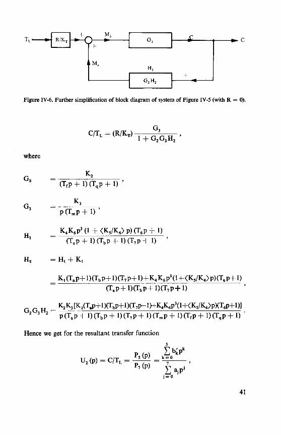
Figure IV-4. Further simplification of block diagram of system of Figure IV-3 (with TL = 0).

38

K2K3K4K6p2 (1 + <KS/K4> p) (T6p + 1)

KjGg =

(Tap + 1) (Tbp + 1) (T7p + 1) (Tmp + 1) (TfP + 1) (Tqp + 1)

K,G7

1 + G7Hj

KiK2K3

p(Tmp + l)(Tfp+l)(Tqp + l)

K2K3K4K6p3 (1 + <K5/K4> p) (T6p + 1)

p(Tap + 1) (Tbp + 1) (T7p + 1) (Tmp + 1) (Tfp + 1) (Tqp + 1)

=

K,K2K3 (TaP + 1) (Tbp + 1) (T7p + 1)

K2K3K4K6p3(l + <K5/K4>p)(T6p+l)+p(Tap+l)(Tbp+l)(T7p+l)(Tmp+l)(Tfp+l)(Tqp+l)-

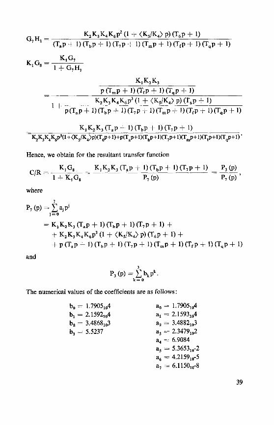
Hence, we obtain for the resultant transfer function

C/R =K'Gs

=

K,K2K3 (Tap + 1) (Tbp + 1) (T7p + 1)=

Pjjp)1+K^ P7(p) P7(p)'

where

P7 (p) = £ a,pij = o

= K,K2K3 (Tap + 1) (TbP + 1) (T7p + 1) +

+ K2K3K4K6p3 (1 + <K5/K4> p) (T6p + 1) +

+ P (TaP + 1) (Tbp + 1) (T7p + 1) (Tmp + 1) (Tf p + 1) (Tqp + 1)

and

P3 (P) = t bkPk_

kfk = 0

The numerical values of the coefficients are as follows :

b0 = 1.7905104 a0 = 1.7905104

bx = 2.1592104 at = 2.1593104

b2 = 3.4868103 a2 = 3.4882103

b3 = 5.5237 a3 = 2.3479102

a4 = 6.9084

a5 = 5.365310-2

a6 - 4.215910-5

a, = 6.1150lft-8

39

In the following we shall denote this transfer function by

I>kPkk=0

U!(P)==^

j = 0

2. Determination of C/T^

When the effect of the load torque disturbances is considered, the position

input R is set equal to zero and the block diagram appears as shown in FigureIV-5. In this figure the feedback function Hx and the error amplification Kxform a parallel grouping of elements, the effective transfer function of which

is called H2. H2 and G2 combine in series to provide the total feedback quantityfor the forward function G3 as shown in Figure IV-6. The process of determin¬

ing C/TL for the block diagram shown in Figure IV-6 becomes analogous to

that for the normal feedback case when it is realised that the polarity of the

feedback quantity is reversed before it appears at the point where it "adds" to

the load torque. The transfer function C/TL is given by

TtR 4 ^

M

CiZ

* Ma

H2

i r

~

1

C iH, * 1 '

G2 46

1 M,K,

N +

11 ^R=0

Figure IV-5. Simplified block diagram of system of Figure IV-2 (with R = 0).

40

TL> R/KT ^fn M3G3 £

T

4

H3

G2H2

Figure IV-6. Further simplification of block diagram of system of Figure IV-5 (with R = 0).

where

Hi

C/TL = (R/KT)1 + G2G3H2

'

K,

(Tfp + l)(TqP+l)'

P(TmP+D

K4K6p3(l + <K5/K4)p)(T6p+D

(Tap+l)(Tbp + l)(T7p+l)

H2 — Ht + Kt

K1(Tap+l)(Tbp+l)(T7p+l)+K4K6p3(l+<K5/K4>p)(Ttp+l)

(Tap+l)(Tbp+l)(T7p+l)

=

K2K3[K1(Tap+l)(Tbp+l)(T7p+l)+K4K6p3(l+<K5/K4>p)(T6p+l)]232

P (Tap + 1) (Tbp + 1) (T7p + 1) (Tmp + 1) (Tfp + 1) (Tqp + 1)

Hence we get for the resultant transfer function

U2(p) = C/TLp,<p) syp7(p)

j = 0

41

where

P5 (p) = (R/KT) K3 (Tap + 1) (Tbp + 1) (T7p + 1) (Tfp + 1) (Tqp + 1)'ql

5

k = 0

and its coefficients are as follows:

b£ = 4.497310-1

b,' = 5.821710-1

b'2 = 1.364210-1

b^ = 8.873510-3

b; = 1.702610-4

b^ = 2.502610-7

The polynominal P7 (p) is exactly the same as in IV. 1.

3. The outputs c (t) corresponding to different inputs on both sides

In the following we shall denote by c, (t) the output corresponding to the

input side R (Figure IV-1), while by c2 (t) that of the input side TL. This is

illustrated in Figure IV-7.

r(t) N aft) —+-c(t) tL (t) H uft) I—+>cft)

\ I

R(p)—»| //Tf/J~]—^(p) T (p)—*\ Ua(p)~\-+Ca(p)

Figure IV-7. Input-output relations.

42

a) Pulse response:

This is the output corresponding to a Dirca-pulse input. In the transform

plane, the input transform becomes

R (P) = TL (p) = 1

and the output transform will be

Cj (p) = U, (p) = j e-ptUj (t) dt, j = 1, 2.

o

Hence, we get for the output

Cfc(t) = u,(t), j = l, 2.

Both transfer functions Uj (p) satisfy the conditions of our inversion method

ofChapter II. Hence, we invert them by this method and obtain the correspond¬

ing pulse responses Cj (t), j = 1, 2, which are shown in Figures IV-8 and IV-9

respectively.

b) Step response:

The Input is given by

f 0 t < 0,

r(t) = tL(t) =

[ 1 t > 0.

The Laplace transform of this function is 1/p so that the output becomes

q (P) = - u, (P)p

=-i + F, (p), j = 1, 2,P

where

and

A! = u, (0)=1,

A2 = uss(0) = 2.511810-5

Fj =

£dkpkk = 0

EamPmm = 0

43

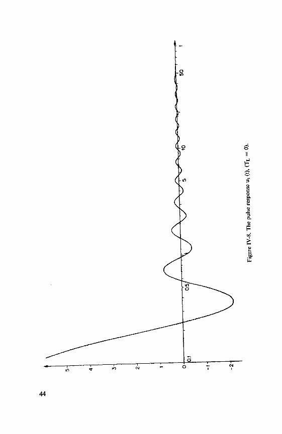
0).

-(TL

(t),

ux

response

puls

eThe

IV-8.

Figure

*

0).

=(R

(t),

u2

response

pulse

The

IV-9.

Figure

Ul*-

F2 = k-^ .

EamPmm = 0

The coefficients in the numerators are as follows:

d0 = -l d; = 3.980510-2

dt = — 1.4044 d; = 4.880710-2

d2 = — 2.2927102 d^ = 2.976110-3

d3 = — 6.9084 ds = — 3.259910-6

d4 = — 5.365310-2 d'4 = — 1.097410-6

d5 = —4.215910-5 ds = —1.058910-9

d6 = -6.114910-8 < = — 1.535910-12

The functions F} (p) are inverted using our method of Chapter II to get their

original functions fs (t) and the resultant outputs become

c, (t) = A, + f, (t), j = l,2.

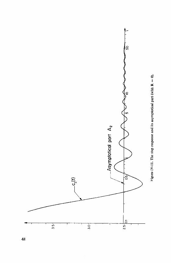
These are drawn, together with their asymptotical parts Aj, in Figures IV-10

and IV-11 respectively.

c) Sinusoidal input:

Let the input be of the form

r(t) = tL(t) = cost.

Its Laplace transform is

R (P) = TL (p) =~j , (poles ± i),

which gives the output transforms

Cs (p) = -^~ U, (p),p2 + 1

whose dominant poles are again ± i. Since the residues, in this case, are

easily computed, we shall not use the method of Chapter III.2 but subtract

the principal part corresponding to them.

46

0).

=TL

(with

part

saymptotical

its

and

response

step

The

IV-10.

Figure

0).

=R

(wit

hpart

asymptotical

its

and

response

step

The

IV-11.

Figure

A: B,

Cj (P) = —j-r + '— + G, (p),p + 1 p —1

where

Aj = juj(-i) =1

y(xi-'yj)

B,= yUj(+i) =i

y (xj + [y)

and

xx = 1.0072 x2 = 2.524210-5

Yl = 5.132710-3 y2 = 2.369310-6

The transforms Gj (p) are as follows:

t^PkG1(p) =

k = 0

7

I>mPmm = 0

6

n (n\ -k = 0

E^p"m = 0

where

e0 = 91.902 <* = 4.242210-2

e1 = — 18.422 ei = 4.893410-2

e2 = — 2.3087102 e2 = 2.964410-3

e3 = — 6.9579 ea = — 3.990210-6

e4 = — 5.403910-2 e; = — 1.103910-6

e5 = — 4.200010-5 e5 = — 1.120010-9

e6 = 0.0000 < = — 1.000010-11

The functions Gj (p) have been inverted by our method of Chapter II to get

gj (t) which add to the asymptotical parts

49

0).

=TL

(with

part

asymptotical

its

and

(t)

Ci

output

The

IV-12.

Figure

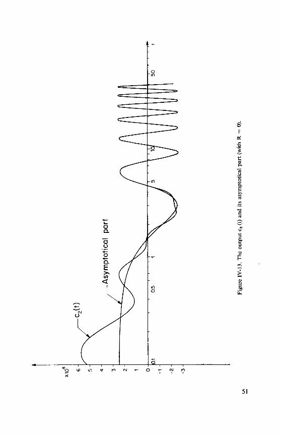
0).

=R

(with

part

asymptotical

its

and

(t)

c2

output

The

IV-13.

Figure

(Xj cost — y; sint)

to give the outputs

Cj (t) = (Xj cost — Vj sint) + % (t), j == 1, 2.

These are shown in Figures IV-12 and IV-13 respectively and are comparedwith their asymptotical parts.

CHAPTER V

Linear Flow of Heat

1. Development of the method (see [9], p. 175)

The homogeneous body - e. g. rod, wall, etc. -, through which the heat

flows in the direction of the x axis, is supposed to occupy the interval (0, a).Both ends, x = 0 and x = a, should always be kept at the constant temperatures

0 and b respectively. Moreover, it will be assumed that at t = 0 a certain

initial distribution F (x) of the temperature is given over the interval (0, a),where naturally F (0) = 0 and F (a) = b. It is required to determine the

temperature U (x, t) at every point x and time t. In addition, U (x, t) should

satisfy the partial differential equation

82U

-G(x)

where c is a given constant and G (x) a given function (of x only). This problemcan be summarised mathematically as follows:

It is required to find a function U (x, t) which satisfies

1. the partial differential equation:d\J a2u

ax2

2. the boundary conditions: i) U (0, t) = 0 and

ii) U (a, t) = b,

and

3. the initial condition: U (x, 0) = F (x).

G(x)

(20)

52

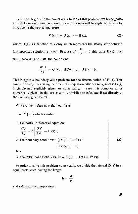
Before we begin with the numerical solution of this problem, we homogeniseat first the second boundary condition - the reason will be explained later - by

introducing the new temperature

V (x, t) = U (x, t) - H (x), (21)

where H (x) is a function of x only which represents the steady state solution

(asymptotical solution, t -» oo). Because of

fulfil, according to (20), the conditions

d2H

0 this state H (x) must

dx2G (x), H (0) = 0, H (a) = b.

This is again a boundary-value problem for the determination of H (x). This

can be done by integrating the differential equation either exactly, in case G (x)is simple and explicitly given, or numerically, in case it is complicated or

numerically given. In the last case it is advisible to calculate H (x) directly at

the points x; given below.

Our problem takes now the new form:

Find V (x, t) which satisfies

1. the partial differential equation:

SV r d2V=c

G(x)

St [ dx2V

\

2. the boundary conditions: i) V (0, t) = 0 and \ (22)

ii) V (a, t) = 0,

and

3. the initial condition: V (x, 0) = F (x) — H (x) = F* (x).

In order to solve this problem numerically, we divide the interval (0, a) in m

equal parts, each having the length

h =m

and calculate the temperatures

53

Vj(t) = V(xj,t)

at the points of division

Xj == jh, j = 1, 2, ...,m— 1

for an arbitrarily chosen time t 2> 0; they are now functions of the time t only.The second derivative appearing in the differential equation will be approx¬

imated numerically by

dx2 h

so that this differential equation could be replaced by the system of ordinary

differential equations

dt= c

V,-, —2V, + Vi + 1— G4 , j = 1, 2, ...,

m —1,

where Gj = G (Xj) and V0 (t) = Vm (t) = 0. Now we introduce the new variable

T = th2

and get the following system

dV,

dT

i= Vj_,-2Vj + Vj+1-h2Gj, j= 1,2, ...,m-l. (23)

For the sake of simplicity, but without restricting the applicability of this

method, we shall put G (x) = 0. In this case the steady state is simply

H (x) = — x.

a

(24)

The last system will then reduce to

dV;i-= Vj_1-2Vj + Vj + 1, j= 1,2, ...,m-l. (25)

54

In order to eliminate the derivative on the left-hand side, we make use of the

Laplace transformation:

-* vj(P)

0 _> v0 (p) ee vm (p) & 0

-> pVj(p) — F*, j = 1, 2, ...,m — 1,

where, according to (24) and the initial condition in (22),

f; = fj--^-xj = fj-Aj, f; = f; = o.a. ill

Therefore, the system (25) will be transformed into

pvj —F* =vj_I— 2Vj + vj + I

or

-vj_1(p) + (2 + p)vj(p)-vj + 1(p)-F;, j = l, ...,m-l. (26)

Since the transforms Vj (p) are all analytic in the right half plane includingthe imaginary axis, we can make use of the method of Chapter II for the deter¬

mination of the initial functions Vj (t) and consequently Uj (t). If the boun¬

dary conditions had not been homogenised, the second would have yielded the

btransform um (p) = — which has a pole at p = 0.

P

Before we begin with the actual inversion, we evaluate at first these trans¬

forms, or, strictly speaking, the functions

Wj (p) = (1 + P) ^ (p), w0 (p) = wm (p) s 0,

at the points

& 2tz

pv = itanv —, # =,

v = 0, 1, ...,n —1.

2 n

Multiplying (26) by (1 + p), putting p = pv and writing

55

V;(T)

V0(T) = Vm(T)

dVj_dx

Wj (pv) = wjv = <xjv + ipjv

we get

—

w(j_1)v + ^2 + itanv~j wjv—w(j + 1)v= Fj M +itanv —

Comparison of real and imaginary parts on both sides yields

0(j-l)v + 2ajv — ao+ i)v— tanv

^' Pjv = Fj

ft ft

Pd-Dv + 2pjv — p0 + 1)v+ tanv — <xjv

= tanv —. F*

(27)

j = 1,2, ..., m—1,

where a0v = (30v = amv = (3mv = 0 for all values of v. The first of these equa¬

tions can be written as

Pjv = cotv —. [— a(j_1)v + 2ajv — a(j+ 1)v— Fi ] (28)

which, when substituted in the second equation, will yield the following system

of linear equations for the determination of the aJV:

&

EaiJaiv = -cos^~.(F*_1-F; + F:+1)+F,*,i=1.2,...,m-l, (29)j=i

where

(a,,) =

/A-C B C \/B A B C 0 |C^

B^

A_

C~~

B

B--„,

C

A'"'

B"'

C

\0 C B A B

C B A-C/

56

A = 5cos2v — + 1, B = — 4cos2v —-

,and C = cos2v —

.The solution of

this system, for every fixed value of v = 0, 1, ...,n — 1, delivers the unknowns

aJV,j = 1, 2, ...,m — 1. The corresponding (3JV are then obtained by direct

substitution in (28). Now the required numerical values of the functions

wj (p)> J = 1> 2, ...,m — 1, at the points of division pv are completely defined.

This is all that is needed for the numerical inversion by the method ofChapter II.

We summarise the steps of calculation as follows (j = 1, 2, ...,m — 1):

The function

w, (p) = (1 + p) Vj (p)

will be transformed by the conformal mapping

1-Pz =

1+P

to give w, (z), which will be approximated by a polynomial of the form

wJ(z)~ngc]kzk.

The coefficients Cjk are calculated by interpolation in the points (the images

0fpv)

zv = e-v».

wJV = ^ (zv) = w, (pv) = aJV + ipjv = £ Cjke ,vk9, v = 0, 1, ...,n — 1

n —1

k = 0

Cjk = - ^ w]Velvk9, k = 0, 1, ...,n—1.n

v = 0

£jk = 9* {Cjk} = - ^(a^cosvk* - pjv sinvkft).n

v = 0

The inverse function of

v](p)=TT7wJ(p)=k?C]k7]-^pT

57

becomes

viW=Y(-i)kwk(2T)k = 0

or, in terms of the original time variable t,

Hence, we get for the resultant temperature (see Relations (21) and (24))

Uj (t) = -^ j +£(- l)k £jk/k (~ t) , j = 1, 2, ...,m- 1.

2. Numerical examples

1. F (x) = x2, a = 4,

m = 4, n = 12.

2. F(x)= sin(yxj ,

m = 4, n = 12.

The results are shown in Figures V-1 and V-2 respectively. The calculated

temperatures Uj (t) approach their respective asymptotical values Uj (oo) with

increasing time t.

b = 16, c = 1.

a = b == c = 1.

58

12

11

10

1.Example

V-1.

Figure

67

6

^

i.^\\

60

Appendix

Program for the Method of Chapter II

A. Formal parameter list

n: Number of divisions.

/: Parameter of the conformal mapping.

r: Radius of the circle in the z plane, on which the division is made

(normal case r = 1).

d: Parallel displacement of the imaginary axis of the transform plane

(normal case d = 0).

10: Begin of the time interval.

delta: Time increment.

11: End of the time interval.

gl, g2: Arrays representing respectively the real and imaginary parts of the

function G (p) at the points of division.

Inform: Procedure which is responsible for printing the instantaneous value

of t and the corresponding value f of f (t).

61

B. ALGOL-program

procedure Lapinversion (n, /, r, d, tO, delta, tl, gl, g2, Inform);

integer n; real /, r, d, tO, delta, tl; array gl, g2; procedure Inform;

begin

integer i, k, j;real theta, p, q, si, s2, t, /0, /l, 12, m ,f;

array xi [0: n — 1], x, y [0: n];theta := 8 x arctan (l)/n;

p:= cos (theta); q := sin (theta);

x[0]:=x[n]:=l;y[0]:=y[n]:=0;

x [1] := x [n — 1] := p; y [1] := q; y [n — 1] :== — q;

for i := 2 step 1 until n/2 do

begin

if n = 4 x i then

begin

x[i] := x[3xi] := 0;

y[i]:= l;y[3xi]:= — 1

end else

if n = 2 x i then

begin

xp]:=-l;y[i]:=-0end else

beginx [i] := x [n — i] := p x x [i — 1] — q x y [i — 1];

y H := (y [i — 1] + q x x [i]) / p; y [n — i] := — y [i]end

end i;

Coefficients:

for k := 0 step 1 until n/2 do

beginsi := s2 := 0;

for i : = 0 step 1 until n — 1 do

begin

j := i x k — entier (i x k/n) x n;

si := si +gl[i] X x[j];s2:= s2 + g2[i] x y [j]

end i;

if k = 0 then xi [0] : = s 1 / n else

if n = 2 x k then xi [k] : = s 1 / (n x r f k) else

62

begin

xi[k]:= (si —s2)/(n x rfk);

xi[n —k] := (si + s2)/(n x r t (n — k))end

end k;

Laguerre:

for t := tO step delta until tl do

begin

/0:=0;/l:=exp((d — I) x t);

m:= — l;f := xi[0] x /l;

for k : = 1 step 1 until n — 1 do

begin72 := ((2 x (k — / x t) — 1) x /l — (k — 1) x 10) / k;

f := f + sign (m) x xi [k] x 12;

m:= — m;/0 := 11; l\ := /2

end k;

Inform (t, f);end Laguerre

end Lapinversion

References

1. Chestnut, H., R. W. Mayer: Servomechanisms and Regulating System Design. Volume 1,

1951.

2. Courant, R., D. Hilbert: Methods of Mathematical Physics. Volume 1, 1953.

3. Doetsch, G.: Handbuch der Laplace-Transformation. 1950.

4. Doetsch, G.: Tabellen zur Laplace-Transformation und Anleitung zum Gebrauch. 1947.

5. Doetsch, G.: Einfuhrung in Theorie und Anwendung der Laplace-Transformation. 1958.

6. Jahnke-Emde-Losch: Tafeln hoherer Funktionen. 1960.

7. Kaczmarz, St., H. Steinhaus: Theorie der Orthogonalreihen. 1935.

8. Lanczos, C: Applied Analysis. 1957.

9. Stiefel, E.: Einfuhrung in die numerische Mathematik. 1961.

10. Szego, G.: Orthogonal Polynomials. 1939.

11. Szego, G.: Ein Beitrag zur Theorie der Polynome von Laguerre und Jacobi. Mathema-

tische Zeitschrift, Band 1 (1918), S. 343-356.

63

Zusammenfassung

Die vorliegende Arbeit behandelt die numerische Riicktransformation einer

auf der imaginaren Achse und in der Halbebene rechts davon analytischen

Laplace-Transformierten. Diese Aufgabe tritt auf bei den praktischen Pro-

blemen der Elektro- und Regelungstechnik, wo der Frequenzgang experimentell

gemessen werden kann. Diese Methode verlangt nur die numerischen Werte

des Frequenzganges fur gewisse Frequenzen.

In Kapitel III ist ein Verfahren fur den Fall entwickelt, wo die Lage (und nur

die Lage) der dominanten Pole bekannt ist. Hier sind wir in der Lage, zugleichden asymptotischen Teil der Zeitfunktion zu gewinnen.

Kapitel IV illustriert die Losungsmethode bei einem praktischen Problem der

Regelungstechnik.

Die Anwendung dieser Methode auf die eindimensionale Warmeleitung ist

in Kapitel V behandelt.

CURRICULUM VITAE

I was born in Alexandria (Egypt) on the 8th of december 1932. There I

visited the primary school for four years and the secondary school for five years.

Afterwards I joined the Faculty of Engineering of the University of Alexandria

and obtained the degree B. Sc. in Electrical Engineering in June 1955. Duringthe following three years I worked as an assistant at the same faculty for the

Department of Mathematics and Physics. In November 1958 I was sent to

Switzerland by the Egyptian government for graduate studies in applied ma¬

thematics. In April 19591 enrolled at the Swiss Federal Institute of Technologyin Zurich (fourth semester - Department of Mathematics and Physics). In

Spring 1962 I obtained the Diploma in Mathematics. Since July 1962 I have

been developing the theory for this thesis at the Institute of Applied Mathe¬

matics using its electronic computer ERMETH for the numerical investigations.

64