incorporating land use impacts on biodiversity into … land use impacts on biodiversity into life...
TRANSCRIPT
UNIVERSITY OF CALIFORNIA
Santa Barbara
Incorporating Land Use Impacts on
Biodiversity into Life Cycle Assessment for the
Apparel Industry
A group project submitted in partial satisfaction of the requirements for the degree of
Master of Environmental Science and Management
for the
Bren School of Environmental Science & Management
By:
Elena Egorova
Heather Perry
Louisa Smythe
Runsheng Song
Sarah Sorensen
Faculty Advisor:
Roland Geyer
April 2014

As authors of this Group Project report, we are proud to archive this report on the
Bren School’s website such that the results of our research are available for all to read.
Our signatures on the document signify our joint responsibility to fulfill the archiving
standards set by the Bren School of Environmental Science & Management.
Elena Egorova
Heather Perry
Louisa Smythe
Runsheng Song
Sarah Sorensen
The mission of the Bren School of Environmental Science & Management is to
produce professionals with unrivaled training in environmental science and
management who will devote their unique skills to the diagnosis, assessment,
mitigation, prevention, and remedy of the environmental problems of today and the
future. A guiding principal of the School is that the analysis of environmental
problems requires quantitative training in more than one discipline and an awareness
of the physical, biological, social, political, and economic consequences that arise
from scientific or technological decisions.
The Group Project is required of all students in the Master of Environmental Science
and Management (MESM) Program. The project is a three-quarter activity in which
small groups of students conduct focused, interdisciplinary research on the scientific,
management, and policy dimensions of a specific environmental issue. This Group
Project Final Report is authored by MESM students and has been reviewed and
approved by:
Faculty Advisor
Roland Geyer
April 2014

iii
Acknowledgements We are grateful for the steadfast guidance we received throughout this project from
our faculty advisor at the Bren School of Environmental Science and Management,
Dr. Roland Geyer. We would like to thank our client, Patagonia, particularly Elissa
Loughman, Corporate Environmental Specialist, and Jill Dumain, Director of
Environmental Strategies for their vision behind this project, their ongoing support, as
well as the opportunity to work with a company pushing the borders of corporate
environmental sustainability. Additionally, this project would not have been possible
without the cooperation of Patagonia’s suppliers.
We would like to thank our external advisors, Dr. Thomas Koellner and Dr. Laura de
Baan, whose research on land use impacts on biodiversity served as the foundation
for this project, and whose expertise was invaluable in shaping this project. We are
also grateful for the expertise provided by Bren School faculty members, Dr. David
Tilman and Lee Hannah, as well as the assistance we received from Giles Rigarlsford
of Unilever N.V. and Christian Schuster of Lenzing AG in obtaining data and
overcoming obstacles throughout the project.
Finally, we are grateful for the continuous support provided by the administrative
staff and community at the Bren School for Environmental Science & Management.

iv
Abstract
The significant amount of land used by the apparel industry contributes to a global
decline in biodiversity. Although land use is a major driver of biodiversity loss, there
is no easily applicable method for incorporating land use impacts on biodiversity into
life cycle assessment (LCA), which means that biodiversity may be neglected in
corporate sustainability decision-making. At the request of Patagonia, Inc., this study
assesses an emerging model attempting to fill this gap. Published by de Baan et al.
(2013b), the model provides a relatively complete set of biodiversity characterization
factors, used to convert a quantity of occupied land into an absolute, regionally
specific measure of potential species loss. We apply the model to four Patagonia t-
shirts to quantify each product system’s biodiversity impacts in order to evaluate
operational limitations and opportunities for the model within the apparel industry.
Although we find that high uncertainty and a broad land use classification scheme
limit the utility of the model, we provide recommendations on how to utilize the
information gleaned from this study to begin analyzing the biodiversity impact of
apparel product systems. Primarily, we identify agricultural- and pastoral-based
processes as primary contributors to biodiversity impact.
v
Table of Contents
Executive Summary ................................................................................................. viii
Definitions .................................................................................................................. xii
1 Objectives & Significance................................................................................... 15
2 Background ......................................................................................................... 18
2.1 Life Cycle Assessment...................................................................................... 18
2.2 Land Use in LCA ............................................................................................. 19
2.3 Measuring Biodiversity ................................................................................... 21
2.3.1 Definition ........................................................................................................... 21 2.3.2 Indicator ............................................................................................................. 22 2.3.3 Spatial Scale ....................................................................................................... 23 2.3.4 Modeling Biodiversity Loss ................................................................................ 24
2.4 Classifying Land Use Types ............................................................................ 24
2.5 Assessed Products ............................................................................................ 25
2.5.1 Cotton ................................................................................................................ 25 2.5.2 Wool .................................................................................................................. 26 2.5.3 Polyester ............................................................................................................ 27 2.5.4 Lyocell ................................................................................................................ 28
3 Methods ................................................................................................................ 29
3.1 Inventory Analysis ........................................................................................... 30
3.1.1 Data Collection .................................................................................................. 30 3.1.2 Elementary Flows .............................................................................................. 31 3.1.3 System Boundary ............................................................................................... 31 3.1.4 Calculating the Inventory Result ........................................................................ 32
3.2 Characterization Factors ................................................................................. 37
3.2.1 Assigning Characterization Factors .................................................................... 38 3.2.2 Adapting Characterization Factors .................................................................... 39
3.3 Impact Assessment ........................................................................................... 43
3.4 Scenario Analysis ............................................................................................. 44

vi
3.4.1 Hypothetical Change of Raw Material Source Location .................................... 44 3.4.2 Impact of Wool Sourcing Assumptions.............................................................. 44
4 Results .................................................................................................................. 46
4.1 Cotton ................................................................................................................ 46
4.2 Wool .................................................................................................................. 46
4.3 Polyester ............................................................................................................ 47
4.4 Lyocell ............................................................................................................... 47
4.5 Background Impacts ........................................................................................ 50
4.6 Uncertainty Analysis ........................................................................................ 50
4.7 Scenario Analysis ............................................................................................. 54
4.7.1 Hypothetical Change of Raw Material Source Location .................................... 54 4.7.2 Testing Assumptions of Raw Wool Impact Assessment .................................... 55
5 Discussion............................................................................................................. 57
5.1 Wide Range of Biodiversity Impacts and Land Occupation ....................... 57
5.2 Importance of Raw Material Production ...................................................... 58
5.3 Influence of the Characterization Factors ..................................................... 58
5.4 Contribution of Electricity Impacts ............................................................... 61
6 Limitations & Conclusions ................................................................................. 63
6.1 Limitation 1: High characterization factor uncertainty............................... 63
6.2 Limitation 2: Cannot capture nuances in land use types ............................. 64
6.3 Limitation 3: Need for location-specific data ................................................ 65
6.4 Limitation 4: Captures limited aspects of biodiversity ................................ 65
6.4.1 Relationship to Conservation Objectives........................................................... 66
6.5 Limitations of the Case Study ......................................................................... 68
7 Recommendations ............................................................................................... 69
7.1 Recommendations for the Model .................................................................... 69
7.2 Recommendations for Patagonia .................................................................... 70

vii
Appendix I ................................................................................................................. 72
Calculating the Characterization Factors .............................................................. 72
Appendix II ................................................................................................................ 74
Supplier Questionnaire for Primary Data Collection ............................................ 74
Appendix III .............................................................................................................. 75
Modeling Species Extinction: SAR vs. EAR ........................................................... 75
References .................................................................................................................. 77

viii
Executive Summary
The global textile and apparel industry requires large inputs of land for raw material
production and fabric manufacturing. Such land use has significant implications for
biodiversity—the diversity of Earth’s species, which provide critical services such as
pollination, water purification, and climate regulation. With global biodiversity loss
estimated at 30% over the last 40 years, the World Wide Fund for Nature (WWF)
asserts that “the loss of biodiversity is, arguably, the greatest threat to stability and
security today” (WWF 2014). Although land use is a major driver of this decline,
there is no easily applicable and industry-wide method for incorporating land use
impacts on biodiversity into life cycle assessment (LCA). Because LCA is a tool used
across a range of industries for evaluating potential environmental impacts of a
product system throughout its life cycle, the inability to easily include biodiversity
loss alongside impacts such as climate change and water use may mean that
companies are underestimating their environmental impacts, and neglecting
biodiversity loss in their decision making. As a company at the frontier of
sustainability, Patagonia commissioned this Bren Group Project to fill that gap so that
Patagonia and other members of the apparel industry are able to make better-informed
decisions and minimize their environmental impacts.
Working iteratively with Patagonia, we evolved the project to cover the following
four objectives:
1. Review existing methodologies for incorporating land use impacts on
biodiversity into LCA, and select a model with high potential for use within
an apparel LCA
2. Quantify the potential land use impacts on biodiversity of four textiles by
applying the selected land use impact assessment model to four Patagonia
product systems
3. Evaluate the effectiveness of the new model for incorporating regional land
use impacts on biodiversity into LCA, and identify limitations and areas of
refinement

ix
4. Assess the potential of this model for use by Patagonia and the apparel
industry in evaluating its product life cycles
Upon review of existing land use LCA methodologies, we selected a promising
model recently developed by de Baan et al. (2013b) based on the completeness and
regional specificity of their published characterization factors for land occupation.
Land occupation prevents the recovery of biodiversity from taking place due to
human land use. Characterization factors provide a score that can be used to convert
an input or output of a product system into a quantifiable impact particular to a
specific impact category, such as biodiversity damage. In this case, the regional
biodiversity characterization factors translate the quantity of land occupied for a
process into an absolute measure of potential species loss based on its land use type
(agriculture, pasture, urban, or managed forest) and ecoregion. Ecoregions are
geographic units defined by patterns of climate, geology, and the evolutionary history
of the planet, thus providing more ecologically relevant information than larger
spatial scales such as biomes. The calculation combines an adapted version of the
Species-Area Relationship (SAR) model, widely used in ecology to measure species
loss, with the methodology outlined by a group of LCA experts in the paper “UNEP-
SETAC guideline on global land use impact assessment on biodiversity and
ecosystem services in LCA.” A similar set of characterization factors previously
published by de Baan et al., measures a relative decrease in species richness between
a particular land use type and a natural reference habitat at the spatial resolution of
biomes (de Baan et al. 2013a). De Baan et al. (2013b) recommend using their updated,
regional characterization factors to obtain an absolute, as opposed to relative
quantification of biodiversity loss in terms of potential species extinction. De Baan et
al. (2013b) assert that these newer characterization factors—those evaluated in this
study—provide a more communicable, socially and politically relevant measure of
biodiversity.
x
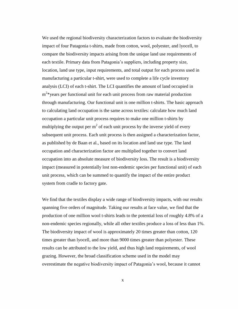
We used the regional biodiversity characterization factors to evaluate the biodiversity
impact of four Patagonia t-shirts, made from cotton, wool, polyester, and lyocell, to
compare the biodiversity impacts arising from the unique land use requirements of
each textile. Primary data from Patagonia’s suppliers, including property size,
location, land use type, input requirements, and total output for each process used in
manufacturing a particular t-shirt, were used to complete a life cycle inventory
analysis (LCI) of each t-shirt. The LCI quantifies the amount of land occupied in
m2*years per functional unit for each unit process from raw material production
through manufacturing. Our functional unit is one million t-shirts. The basic approach
to calculating land occupation is the same across textiles: calculate how much land
occupation a particular unit process requires to make one million t-shirts by
multiplying the output per m2 of each unit process by the inverse yield of every
subsequent unit process. Each unit process is then assigned a characterization factor,
as published by de Baan et al., based on its location and land use type. The land
occupation and characterization factor are multiplied together to convert land
occupation into an absolute measure of biodiversity loss. The result is a biodiversity
impact (measured in potentially lost non-endemic species per functional unit) of each
unit process, which can be summed to quantify the impact of the entire product
system from cradle to factory gate.
We find that the textiles display a wide range of biodiversity impacts, with our results
spanning five orders of magnitude. Taking our results at face value, we find that the
production of one million wool t-shirts leads to the potential loss of roughly 4.8% of a
non-endemic species regionally, while all other textiles produce a loss of less than 1%.
The biodiversity impact of wool is approximately 20 times greater than cotton, 120
times greater than lyocell, and more than 9000 times greater than polyester. These
results can be attributed to the low yield, and thus high land requirements, of wool
grazing. However, the broad classification scheme used in the model may
overestimate the negative biodiversity impact of Patagonia’s wool, because it cannot
xi
capture the sustainable grazing strategies used by the t-shirt’s suppliers. Additionally,
we find that raw material production contributes more than 99% of the total
biodiversity impact and land occupation for the cotton and wool t-shirts, and 92% of
the lyocell t-shirt. These textiles require agriculture-, forest-, and pasture-based land
uses, which have significantly lower yields, and thus require more land per unit, than
the urban manufacturing processes. While the biodiversity impacts of cotton and wool
manufacturing are dominated by the land occupation required for those processes, the
impacts of polyester and lyocell are influenced by the characterization factors.
In its present form, the model is limited by four primary factors. First is the high
uncertainty present in the characterization factors, as calculated by de Baan at al.;
using characterization factors for the upper and lower bounds of a 95% confidence
interval produces over a 100% change in the biodiversity impact of all evaluated
textiles, and over 1700% change in the case of polyester. Second, the coarse land use
classification means that users are unable to differentiate between land use
management strategies, such as organic versus conventional cotton. Third, to take full
advantage of the model requires location-specific knowledge of manufacturing
processes, which may not be available to companies that rely on commodity products
or lack transparency in their supply chains. Finally, one model may never be able to
sufficiently quantify impacts on biodiversity, due to the complex nature of
biodiversity. While these characterization factors essentially rely on species richness,
or the number of species in a given area, the concept of biodiversity can also include
species distribution, genetics, ecosystem functioning, and a range of other factors.
Although this model has potential for future use in LCAs alongside other indicators,
we find that currently it is better suited for providing generalizations about relative
biodiversity impacts rather than for conducting discrete product system assessments.
The continued refinement and development of methods for incorporating biodiversity
impacts into LCA will greatly improve the ability of companies to make
environmentally-informed decisions about product systems.
xii
Definitions
Biodiversity
Biodiversity is the totality of genes, species and ecosystems of a region (Davis 2008).
This term is often used to refer to genetic diversity, species diversity, and ecosystem
diversity.
Biodiversity Impact
As used in this study, biodiversity impact is the result of the impact analysis,
measured in potentially lost non-endemic species per functional unit. It is the
biodiversity loss resulting from land occupation for human activities adjusted for the
location and land use type of those activities.
Characterization Factor (CF)
Used in life cycle assessment, a characterization factor converts an assigned life cycle
inventory analysis result to the common unit of the impact category indicator (ISO
2006E).
Ecoinvent
Ecoinvent is a professional database containing life cycle inventory data from a range
of industries, such as data on energy supply, resource extraction, material supply,
chemicals, metals, agriculture, waste management services and transport services that
can be imported into life cycle assessment. It is developed and maintained by the
Swiss Centre for Life Cycle Inventories.
Ecosystem Services
Ecosystem services are the benefits humans derive from wildlife and ecosystems,
such as provisioning of food; regulation of climate and disease; support of the
nutrient cycle and crop pollination; as well as cultural, spiritual and recreational
benefits.
Elementary Flow
The material or energy of the studied system that has been drawn from the
environment without previous human transformation, or the material or energy
leaving the studied system that is released into the environment without subsequent
human transformation (ISO 2006E).

xiii
Functional Unit
The functional unit is a pre-determined quantity of the product or service being
evaluated in the life cycle assessment. It provides a basis for the comparison of
performance between product systems.
GaBi
GaBi is a professional life cycle assessment modeling software developed and
maintained by PE international. It integrates multiple databases to allow the user to
develop a life cycle assessment model.
Impact Category
A class representing environmental issues of concern to which life cycle inventory
analysis results may be assigned (ISO 2006E). The selected category represents the
aspects of environmental impact that a life cycle assessment is interested in
measuring. Classic impact categories include global warming potential,
eutrophication, acidification, and human toxicity potential.
Impact Category Indicator
The impact category indicator is a quantifiable representation of an impact category
(ISO 2006E). Each impact category has an indicator to characterize its impact.
Land Occupation
One of two types of land use interventions typically considered in life cycle
assessment, land occupation is the continued use of land for human use, which
prevents the land from recovering to a natural state (de Baan et al. 2013a).
Land Transformation
One of two types of land use interventions typically considered in life cycle
assessment, land transformation, or land use change, alters the characteristics of a
piece of land in order to make it suitable for a new use (Koellner 2013).
Life Cycle Assessment (LCA)
LCA is a method of compiling and evaluating “the inputs, outputs and the potential
environmental impacts of a product system throughout its life cycle” (ISO 2006 E). It
consists of four major phases: goal and scope definition, life cycle inventory analysis,
life cycle impact assessment, and life cycle interpretation.
Life Cycle Impact Assessment (LCIA)

xiv
LCIA is the phase of LCA “aimed at understanding and evaluating the magnitude and
significance of the potential environmental impacts for a product system throughout
the life cycle of a product” (ISO 2006E). The results of the life cycle inventory
analysis are assigned to particular areas of environmental concern, or impact
categories.
Life Cycle Inventory Analyses (LCI)
LCI is the phase of LCA in which inputs and outputs of a product system are
quantified through data collection and analysis (ISO 2006E).
15
1 Objectives & Significance
The textile and apparel industry is global and rapidly growing; American consumers
alone spend $360 billion on clothes and shoes every year (AAFA 2014). Wool
produced in the Patagonian grasslands of South America may be spun into yarn in
China, sewn into a t-shirt in Vietnam, and worn by a consumer in the Unites States.
The industry requires massive inputs of chemicals such as dyes and fertilizers, water,
and energy, and contributes significantly to air and water pollution, climate change,
and other environmental problems. In order to better understand and address the
substantial impacts that the industry has on the quality of Earth’s ecosystems,
companies and researchers are using Life Cycle Assessment (LCA) as a tool to
measure the potential environmental impacts of a particular product system
throughout its life cycle—from raw material extraction to consumer use and product
disposal.
While certain impacts, such as those to global warming, are readily incorporated into
LCAs with standardized practices, methodologies for other impacts still need to be
developed. In particular, there is currently no easily accessible and widely applicable
LCA method for quantifying the impacts of land use on biodiversity—the diversity of
Earth’s species—even though land use is one of the major causes of biodiversity loss
(de Baan 2013b). According to the World Wide Fund for Nature (WWF), “the loss of
biodiversity is, arguably, the greatest threat to stability and security today.” Although
researchers estimate that there are roughly 8.7 million different species on Earth
(Mora et al. 2011), global biodiversity has declined roughly 30% over the last 40
years (WWF 2014). Should biodiversity continue to decline at this rate, critical
ecosystem services (services provided by the environment such as pollination, water
purification, carbon sequestration, and soil formation) will be lost. Conversion of
natural land for human use leads to decreased, modified, and fragmented habitats, in
addition to degraded soil and water quality, and the exploitation of native species, all
16
of which contribute considerably to biodiversity loss (Foley 2005). The inability to
easily include biodiversity loss alongside impacts such as climate change and water
use using LCA likely means that companies are underestimating their environmental
impacts, and neglecting biodiversity loss in their decision making. Developing and
propagating a method for incorporating land use impacts on biodiversity into LCA
will increase awareness on the critical issue of global biodiversity decline, and enable
companies to better minimize their environmental impacts.
Patagonia, Inc. (Patagonia), an outdoor apparel and gear company that has been a
pioneer in sustainable manufacturing for more than 30 years, recognizes that they
have a role to play in curtailing biodiversity loss, and are actively seeking ways to
incorporate land use impacts into their life cycle assessments to make better-informed
decisions. To this end, Patagonia commissioned a Bren Group Project to identify
existing LCA land use impact methodologies, and pilot one of these methodologies
using Patagonia’s product supply chains to evaluate its effectiveness and make
recommendations. Working iteratively with Patagonia, we evolved the project to
cover the following four objectives:
1. Review existing methodologies for incorporating land use impacts on
biodiversity into LCA, and select a model with high potential for use within
an apparel LCA
2. Quantify the potential land use impacts on biodiversity of four textiles by
applying the selected land use impact assessment model to four Patagonia
product systems
3. Evaluate the effectiveness of the new model for incorporating regional land
use impacts on biodiversity into LCA, and identify limitations and areas of
refinement
4. Assess the potential of this model for use by Patagonia and the apparel
industry in evaluating its product life cycles
In addition to evaluating an emerging LCA methodology, this study provides
Patagonia with a first-order assessment of the land use impacts of its common textiles,

17
as well as a potential tool for future assessments. Because Patagonia does not own
and operate its own manufacturing facilities, it is difficult to maintain complete
visibility of its supply chain impact across the globe. By capturing data directly from
the supply chain, this study will increase Patagonia’s awareness of its global impacts,
all the way down to its raw material suppliers and manufacturers. Patagonia can then
apply this knowledge to inform decisions, and outline appropriate actions to take to
minimize the impacts of its land use on biodiversity.
Furthermore, Patagonia has the ability to motivate industry-wide change in
sustainability practices, so the significance of this project goes beyond assessing one
company’s impacts. Led by innovative companies such as Patagonia, the apparel
industry is uniting through the Sustainable Apparel Coalition (SAC) to advance
corporate sustainability efforts. The mission of the SAC is to create “a common
approach for measuring and evaluating apparel and footwear product sustainability
performance that will spotlight priorities for action and opportunities for
technological innovation” (SAC 2014). Establishing a consistent measure for land use
impacts on biodiversity is a critical addition to that common approach. Patagonia can
use the SAC as a forum to share the findings of this study, and enable other
companies to evaluate and reduce their own impacts on biodiversity.

18
2 Background
2.1 Life Cycle Assessment
Life Cycle Assessment (LCA) is a valuable tool used to evaluate the potential
environmental impacts of a product system throughout its life cycle. As outlined in
International Standard 14040 established by the International Standard Organization
(ISO), LCA consists of four phases: Goal and Scope Definition, Life Cycle Inventory
Analysis (LCI), Life Cycle Impact Assessment (LCIA), and Interpretation. LCA is an
iterative process, with interpretation being conducted throughout to identify necessary
adjustments in the goal, scope, and subsequent phases (ISO 2007).
At the core of an LCA is the functional unit, which quantifies the product(s)
function(s) and serves as a common reference unit that enables comparison of results
across equivalent product systems. In this study, the functional unit will allow us to
compare the potential land use impacts of the four textile types we will be evaluating,
each represented by a specific Patagonia t-shirt. The functional unit, as well as the
reference flow (the amount of product(s) required to fulfill the intended function
defined by the functional unit) and the system boundary are established in the first
phase. During the LCI phase, inputs from and outputs to the environment, called
elementary flows, of the product system are quantified through data collection (such
as energy inputs, waste, emissions to air) and data calculation. In the LCIA, the
results of the LCI are assigned to particular areas of environmental concern called
impact categories, which are quantifiably represented by an impact category
indicator. Characterization factors derived from a characterization model are used to
convert the LCI results into indicator results summed for each impact category. In
this way, the LCIA measures the potential environmental impacts of the specific
inputs and outputs of the product system. For example, if CO2 is an output in the LCI,
it could be assigned to the impact category “global warming,” which might be

19
represented by the category indicator “infrared radiative forcing,” and converted
using the characterization factor “Global Warming Potential” into a category
indicator result represented in units of kg-CO2-equivalent (ISO 2007). The LCA
elements used in this study are summarized in Table 1.
Table 1. LCA elements used to complete this study
Impact Category Potential Biodiversity Loss
Elementary Flow Land occupation Unit: square meters * years per functional unit
Characterization Factors
Convert land occupation to regional biodiversity loss Unit: potentially lost non-endemic species for occupying one square meter for one year
Functional Unit One million t-shirts
Indicator Result Biodiversity Impact Unit: potentially lost non-endemic species per functional unit
2.2 Land Use in LCA
An international group of LCA experts recently completed the Land Use Life Cycle
Impact Assessment (LULCIA) project (Koellner et al. 2013), which establishes an
operational method for incorporating land use impacts on biodiversity and ecosystem
services into LCA. The work of the LULCIA team is published in a Special Issue of
the International Journal of Life Cycle Assessment called Global Land Use Impacts
on Biodiversity and Ecosystem Services in LCA. The LULCIA initiative is one piece
of the broader UNEP-SETAC International Life Cycle Initiative, a partnership
formed by the United Nations Environment Programme (UNEP) and the Society for
Environmental Toxicology and Chemistry (SETAC).
Our study drew heavily on the founding work of the UNEP-SETAC Life Cycle
Initiative, as published in the article “UNEP-SETAC guideline on global land use
impact assessment on biodiversity and ecosystem services in LCA” in the Special
Issue of the International Journal of Life Cycle Assessment. This study establishes a

20
framework for assessing impacts to biodiversity and ecosystems services as a result of
land use. The UNEP-SETAC guideline identifies three land use interventions, which
can be accounted for as elementary flows in the Life Cycle Inventory: land
transformation, land occupation, and permanent impacts. Land transformation refers
to a change in land use, such as conversion from forest to agriculture, while
occupation is the ongoing use of a parcel of land, for example as an agricultural field,
which prevents the land from returning to a natural state. Permanent impacts imply
irreversible changes to the ecosystem (Koellner et al. 2013).
Building from the UNEP-SETAC guidelines, de Baan et al. developed a regional
biodiversity characterization factor model, and calculated characterization factors for
land occupation, transformation, and permanent impacts, as published in “Land use in
life cycle assessment: global characterization factors based on regional and global
potential species extinction” in the journal Environmental Science and Technology
(de Baan et al. 2013b). Our study applies and evaluates the published regional
biodiversity characterization factors for land occupation, which convert land
occupation into the category indicator result measured in absolute units of
“potentially lost non-endemic species,” referred to throughout our results as
biodiversity impact. Whereas de Baan et al. (2013a) previously published
characterization factors for local, relative species losses, in the latest publication de
Baan et al. (2013b) provide an absolute measure of biodiversity loss due to land use
with impacts calculated at a regional scale. The previously published characterization
factors measure a relative decrease in species richness between a particular land use
type and a natural reference habitat at the broader spatial resolution of biome (de
Baan et al. 2013a). These characterization factors are incorporated into the calculation
of the new regional characterization factors as a species sensitivity factor, or relative
decrease in species richness (see Eq. 4 in Appendix I). De Baan et al. (2013b) assert
that the more recently published characterization factors, those used in this study,
provide a more communicable, socially and politically relevant measure of
biodiversity. De Baan et al. (2013b) recommend using their updated, regional

21
characterization factors to obtain an absolute, as opposed to relative, quantification of
biodiversity loss in terms of potential species extinction. Greater detail on the model
used to generate these characterization factors is provided in Appendix I.
Finally, our study draws upon a case study conducted by Milà i Canals et al. (2012) of
the land use impacts on biodiversity and ecosystem services of margarine in the
United Kingdom and Germany. This article was also published in the Special Issue,
and is one of the few available case studies demonstrating the potential applicability
of the framework developed by the LULCIA initiative. The authors define their
system boundary to exclude the distribution process and any processes downstream of
it, but do include certain background impacts. The study uses seven different impact
categories, including biodiversity damage potential, which was measured using the
older set of local land occupation characterization factors developed by de Baan et al.
(2013a), as well as transformation characterization factors calculated by the authors.
2.3 Measuring Biodiversity
Biodiversity is a complex and multi-faceted concept, which may be valued in many
different ways. To complete a study considering biodiversity requires the complicated
tasks of choosing an appropriate definition for biodiversity; selecting an appropriate
indicator; and establishing the spatial resolution at which biodiversity is to be
measured based on one’s objectives and data availability. Each of these decisions
leads to certain tradeoffs.
2.3.1 Definition
The concept of biodiversity is intricate and pluralistic. Attempts to define the term
have led to controversy among ecologists over whether “diversity” should be
quantified with an absolute species count, or if “diversity” should also capture genetic
diversity, species abundance and spatial distribution, functional elements within
ecosystems, or the relative importance of a particular species to an ecosystem.

22
Franklin et al. (1981) recognized three attributes of biodiversity in a region:
composition, structure, and function, together providing a comprehensive picture of a
region’s biodiversity. Although no single definition of biodiversity captures all of its
integrated parts, and its measurement is dependent on the values and conservation
priorities of the decision-maker (Faith 2008), one widely accepted definition of
biodiversity is “the variety and variability among living organisms and the ecological
complexes in which they occur” (OTA 1987). The characterization factors used in
this study are based on the measurement of biodiversity using species richness, or the
absolute count of different species within a particular area.
2.3.2 Indicator
Measurable indicators exist for the aforementioned biodiversity attributes for multiple
levels of organization: regional landscape, community-ecosystem, population-species,
and genetics (Noss 1990). Noss (1990) lists species richness as one appropriate
indicator for assessing terrestrial biodiversity at the level of regional landscape. In the
context of LCA, six potential biodiversity indicators related to species richness have
been identified (summarized in Table 2): alpha diversity, Fisher’s alpha, Shannon’s
entropy, Sorensen’s S, and Mean Species Abundance (de Baan et al. 2013a). In their
earlier calculation of local characterization factors of biodiversity impacts at the
biome level, de Baan et al. (2013a) chose alpha diversity as their indicator due to its
simplicity, data availability, and wide use. Although potential species extinction is
used as the measure of biodiversity loss in the latest de Baan et al. (2013b) regional
characterization factors, alpha diversity is incorporated through the “sensitivity of the
species group to all land use types” variable (see Appendix I and Section 2.3.4 for
more about this calculation). The species richness values in the characterization
factors are taken from WWF and based on extant species ranges (de Baan et al.
2013b).

23
Table 2. Proposed Biodiversity Indicators, adapted from de Baan et al. (2013a)
Indicator Measures Data Requirements Additional Information
Alpha Diversity Species Richness
Species numbers Gives equal weight to all species; highly dependent on sampling
Fisher’s Alpha Species Richness
Species numbers, total number of individuals
Corrects for incomplete sampling of Alpha Diversity
Shannon’s entropy, H
Diversity List of species, relative abundance
Reaches maximum when all species in a sample area are equally abundant
Sorensen’s S Dissimilarity List of species Values between 0 and 1
Mean Species Abundance
Abundance List of current species, list of original species, relative abundance
Changes in abundance of each species between reference and current habitat
2.3.3 Spatial Scale
Biodiversity can be measured based on a number of spatial classifications, such as
biomes, continents, and countries. The characterization factors calculated by de Baan
et al. (2013b) consider biodiversity at the level of ecoregions, defined as “relatively
large units of land containing a distinct assemblage of natural communities and
species, with boundaries that approximate the original extent of natural communities
prior to major land-use change” (Olson et al. 2001). Ecoregions take into account
patterns of climate, geology, and the evolutionary history of the planet, thus providing
more ecologically relevant results in these characterization factors than those
previously developed using larger spatial scales such as biomes.
Olson et al., in conjunction with the World Wide Fund for Nature (WWF), utilized
data from regional experts and biogeographic maps to breakdown 8 biogeographic
regions and 14 biomes into 867 ecoregions. Through extensive exploration of
regional systems by experts in each of the biomes, Olson et al. were able to adapt
ecoregion boundaries from regional classification systems. Where widely accepted
24
biogeographic maps were unavailable, Olson et al. used landform and vegetation
information to develop ecoregion boundaries.
2.3.4 Modeling Biodiversity Loss
The species-area relationship (SAR) is widely used in ecology as an indirect means to
predict species extinction due to habitat loss. The SAR model can be used to calculate
the number of species in a new habitat area as a function of the number of species in
the original habitat area (de Baan et al. 2013b). Some ecologists argue that estimating
extinction based on the SAR method overestimates extinction rates by as much as 160%
in some cases because the model assumes that “any loss whatsoever of population
due to habitat loss commits a species to extinction,” which is an oversimplification of
how ecosystems function (He and Hubbell 2011), as species can persist on human-
modified land (the “matrix”). Therefore, in calculating the characterization factors
used by this study, de Baan et al. (2013b) use a matrix-calibrated SAR model
developed by Koh & Ghazoul (2010) to measure species richness. The matrix SAR
aims to correct for the shortcomings of the SAR model by adding terms that account
for taxon-specific responses to individual components of the matrix and edge effects,
thereby lowering predicted species extinction risk (de Baan et al. 2013b). A more
detailed explanation of how this model was used to calculate the characterization
factors used in this study is provided in Appendix I, while Appendix III provides a
deeper look into the SAR.
2.4 Classifying Land Use Types
Despite the extensive list of global land use and land cover maps available, there is
significant lack of agreement between specific types and locations of land cover and
distribution. For this reason, de Baan et al. (2013b) delineate four broad land use
categories. The land use types agriculture, pasture, managed forest, and urban are
distinguished for each ecoregion based on two maps, the Land Degradation
Assessment in Drylands (LADA, 1998-2008) and Anthromes (2000-2005) based on

25
remote sensing and human statistics data (de Baan et al. 2013b). Although the earlier
set of characterization factors by de Baan et al. (2013a) are regionalized at a coarser
spatial resolution than the new set of characterization factors, they are based on a
finer resolution land use classification system. For example, the land use activity
“agriculture” in de Baan et al. (2013a) is further subdivided into arable and permanent
crops, irrigated and non-irrigated, extensive and intensive, based on the Global Land
Cover project (Bartholomé 2005) and the Global Biodiversity Model (Koellner et al.
2012). Unfortunately, due to lack of sufficient data across many land use categories,
the previous set of characterization factors was far less complete than the newer set
from de Baan et al. (2013b). Thus in choosing the new set of characterization factors,
we lose the ability to distinguish between specific land use activities, in favor of a
more complete set of regionally-specific characterization factors.
2.5 Assessed Products
In designing our study, we determined that using a life cycle assessment approach to
calculate the biodiversity impact of land use for four textiles (wool, polyester, cotton,
and lyocell) would prove most useful in fulfilling our project objectives, because
these textiles can be expected to have markedly different impacts due to their unique
land use requirements. In collaboration with Patagonia’s representatives, we selected
four Patagonia t-shirts of comparable weight and similar style, which each represent
one of the four textiles evaluated in this study. The selected products and initial
product data are described below for each material.
2.5.1 Cotton
Patagonia’s Men’s Sunset Logo T-shirt is used to represent cotton in this
study. Patagonia uses only 100% organic cotton in all of their product
lines (Patagonia 2013). Patagonia’s cotton supply chain for this t-shirt
consists of five unit processes. First, Texas Co-op, a farming cooperative in Texas,
grows raw organic cotton, which is sent to a nearby ginning facility, where the cotton

26
fiber is separated from the cottonseed, burrs, and trash. The cotton fiber represents
approximately 80% of the profits from raw cotton, while cotton seed and other co-
products account for 20% (Texas Co-op 2014). The ginned fiber is then spun into
yarn at a facility in Mexico. An integrated facility in Mexico completes the remainder
of the processes required to turn the yarn into a completed t-shirt, including knitting
yarn into fabric, dyeing and finishing, and cutting and sewing the final t-shirt.
Figure 1. Process flow diagram of the cotton product system
2.5.2 Wool
The Women’s Merino 1 Silkweight T-shirt represents wool. Although the
t-shirt is made of 65% Merino wool and 35% Capilene, our inventory and
calculations were completed as though the shirt were made from 100%
wool based on available data and the objectives of the study. The wool for this shirt is
supplied by Ovis XXI in Argentina. Patagonia has formed a partnership with Ovis
XXI and The Nature Conservancy to utilize Grassland Regeneration and
Sustainability Standard (GRASS) grazing practices, which are intended to restore
natural grasslands in South America. More information about Patagonia’s sustainable
grazing partnership with Ovis XXI, the wool supplier, can be found in Section 5.1.
With respect to Patagonia’s supply chain, approximately 70% of the profits of sheep
grazing come from wool production, while 30% come from the sale of sheep meat, or
mutton (Ovis XXI 2014). The supply chain for this t-shirt consists of five unit
processes, beginning with shearing sheep to produce raw fiber in Argentina. Another
Argentine facility scours the wool to remove grease and dirt, then combs it to separate
the longer fibers from the shorter fibers to create “top”. Top is then sent to a spinning
Raw Material Agriculture
United States (TX)
Ginning Urban
United States (TX)
Spinning Urban Mexico
Knitting/Sewing Urban Mexico

27
facility in China where it is turned into yarn, which is knitted into fabric in Thailand.
Finally, the fabric is cut and the final t-shirt is sewn at a facility in Vietnam.
Figure 2. Process flow diagram of the wool product system
2.5.3 Polyester
Polyester is represented by the Men’s Polarized Tee, made of 100%
virgin polyester. Virgin polyester is a synthetic fiber derived from
petroleum and natural gas. Six unit processes were assessed for
Patagonia’s polyester shirt, including raw material extraction, polymer to fiber
production, spinning, knitting, cutting, and sewing. Patagonia’s polyester polymers
and staple fibers for this t-shirt are produced in South Carolina, then drawn
(stretching the fiber) and spun into yarn at a plant in North Carolina. The yarn is knit
into a fabric at a Los Angeles facility, where it is also dyed and finished. The final
cutting and sewing of the shirt is done in El Salvador. Due to the nature of a
commodity product such as petroleum, it is impossible to trace the specific origins of
this product.
Figure 3. Process flow diagram of the polyester product system
Raw Material Pasture
Argentina
Top Production
Urban Argentina
Spinning Urban China
Knitting Urban
Thailand
Cutting/Sewing Urban
Vietnam
Raw Material Mixed
Ecoinvent Data
Staple Fiber Production
Urban United States (SC)
Spinning Urban
United States (NC)
Knitting Urban
United Sates (CA)
Cutting/Sewing
Urban
El Salvador
28
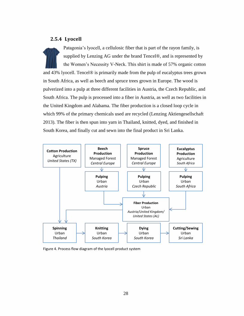
2.5.4 Lyocell
Patagonia’s lyocell, a cellulosic fiber that is part of the rayon family, is
supplied by Lenzing AG under the brand Tencel®, and is represented by
the Women’s Necessity V-Neck. This shirt is made of 57% organic cotton
and 43% lyocell. Tencel® is primarily made from the pulp of eucalyptus trees grown
in South Africa, as well as beech and spruce trees grown in Europe. The wood is
pulverized into a pulp at three different facilities in Austria, the Czech Republic, and
South Africa. The pulp is processed into a fiber in Austria, as well as two facilities in
the United Kingdom and Alabama. The fiber production is a closed loop cycle in
which 99% of the primary chemicals used are recycled (Lenzing Aktiengesellschaft
2013). The fiber is then spun into yarn in Thailand, knitted, dyed, and finished in
South Korea, and finally cut and sewn into the final product in Sri Lanka.
Figure 4. Process flow diagram of the lyocell product system
Beech Production
Managed Forest Central Europe
Eucalyptus Production Agriculture South Africa
Cotton Production Agriculture
United States (TX)
Pulping Urban
Czech Republic
Pulping Urban
South Africa
Spruce Production
Managed Forest Central Europe
Fiber Production Urban
Austria/United Kingdom/ United States (AL)
Spinning Urban
Thailand
Knitting Urban
South Korea
Dying Urban
South Korea
Cutting/Sewing Urban
Sri Lanka
Pulping Urban Austria

29
3 Methods
This case study seeks to quantify the impacts of land occupation on biodiversity using
characterization factors developed by de Baan et al. (2013b). Figure 5 provides a
conceptual overview of the study methods.
In short, industry data and primary data from Patagonia’s suppliers are combined in
the life cycle inventory analysis (LCI) to calculate a land occupation inventory result
for every unit process of each of the four textiles. In parallel, a characterization factor
is assigned to each unit process based on its land use type and ecoregion, which was
determined using GIS mapping. In the life cycle impact assessment (LCIA), the
inventory results are combined with the assigned characterization factors to convert
the LCI results into a measure of biodiversity loss due to land occupation. Scenario
analyses were conducted to better understand the model, and to provide a deeper
analysis of the results. To allow for the comparison of land use impacts of the four
textiles of interest (wool, lyocell, cotton, and polyester) represented by Patagonia
Figure 5. Conceptual overview of the study methods
Background Electricity Data
from Ecoinvent & Literature
Inventory Analysis
Foreground Data
from Patagonia Suppliers
Characterization Factors from de Baan et al.
GIS Mapping
Impact Assessment
Scenario Analysis
Conclusion

30
products, we defined the functional unit of this study as one million medium sized t-
shirts. This value is a realistic approximation of an apparel company’s annual product
output. Because LCA is a linear model, the results can be easily scaled to any
functional unit (e.g. one t-shirt or ten thousand).
3.1 Inventory Analysis
The life cycle inventory analysis (LCI), is the phase of a life cycle assessment
involving the compilation and quantification of inputs and outputs for a given product
system throughout its life cycle (ISO 2007). Using the primary data collected from
Patagonia’s suppliers, supplemented with secondary data, we calculated how much
land occupation each unit process requires to manufacture one million t-shirts.
3.1.1 Data Collection
In order to collect primary data specific to each t-shirt supply chain, questionnaires
were sent to Patagonia’s suppliers soliciting data such as property size, facility size,
location (address or coordinates), land use type, duration of land use, textile input
requirements, total output, and yield. A sample questionnaire is shown in Appendix II.
Literature and the Ecoinvent 2.0 database were used to supplement any data that was
unavailable through Patagonia’s suppliers, such as the purified Terephthalic acid
(PTA) and ethylene glycol inputs of polyester, as well as background electricity data.
According to the Ecoinvent website, the database is “the world’s leading supplier of
consistent and transparent, up-to-date Life Cycle Inventory (LCI) data”. Ecoinvent
supplies information collected from a range of industries from agriculture to energy
supply to packaging materials (Ecoinvent Centre 2014). It is one of the few databases
containing land occupation elementary flows. The data provided in the Ecoinvent 2.0
database are mostly collected from companies in Europe. Specifically, we use
Ecoinvent to supply data for land use requirements of amorphous PET, an input for
the production of polyester fabric, and the background process of electricity.
31
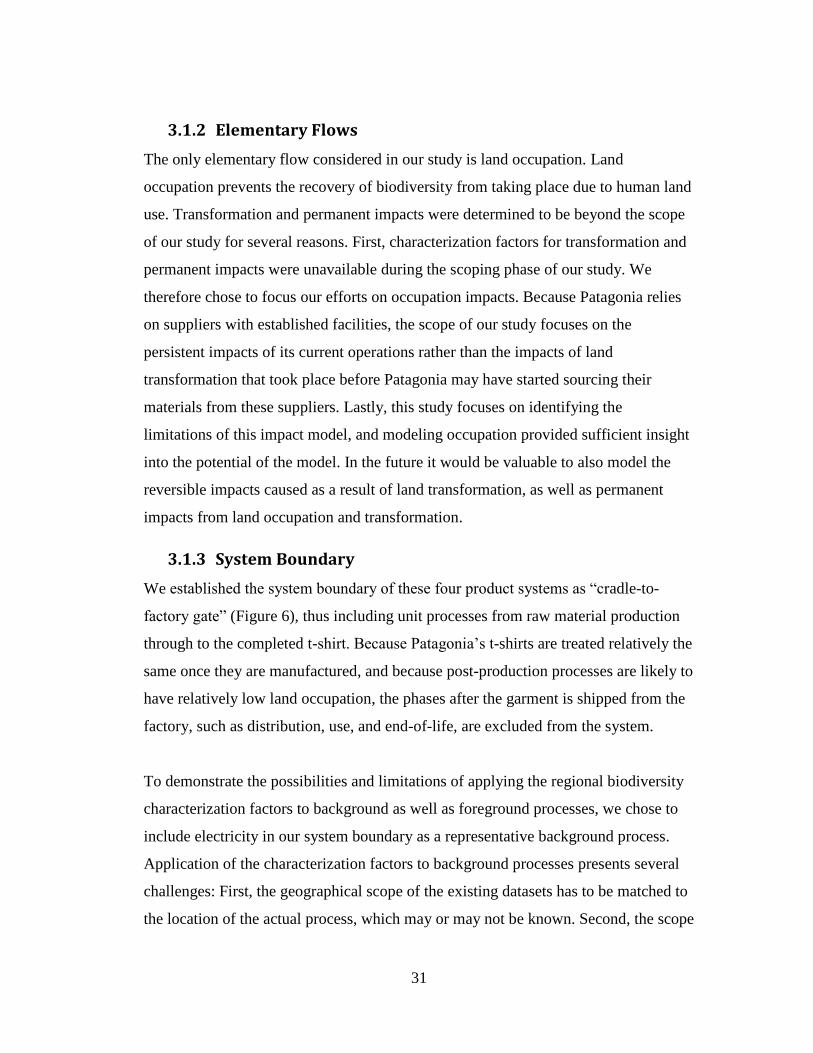
3.1.2 Elementary Flows
The only elementary flow considered in our study is land occupation. Land
occupation prevents the recovery of biodiversity from taking place due to human land
use. Transformation and permanent impacts were determined to be beyond the scope
of our study for several reasons. First, characterization factors for transformation and
permanent impacts were unavailable during the scoping phase of our study. We
therefore chose to focus our efforts on occupation impacts. Because Patagonia relies
on suppliers with established facilities, the scope of our study focuses on the
persistent impacts of its current operations rather than the impacts of land
transformation that took place before Patagonia may have started sourcing their
materials from these suppliers. Lastly, this study focuses on identifying the
limitations of this impact model, and modeling occupation provided sufficient insight
into the potential of the model. In the future it would be valuable to also model the
reversible impacts caused as a result of land transformation, as well as permanent
impacts from land occupation and transformation.
3.1.3 System Boundary
We established the system boundary of these four product systems as “cradle-to-
factory gate” (Figure 6), thus including unit processes from raw material production
through to the completed t-shirt. Because Patagonia’s t-shirts are treated relatively the
same once they are manufactured, and because post-production processes are likely to
have relatively low land occupation, the phases after the garment is shipped from the
factory, such as distribution, use, and end-of-life, are excluded from the system.
To demonstrate the possibilities and limitations of applying the regional biodiversity
characterization factors to background as well as foreground processes, we chose to
include electricity in our system boundary as a representative background process.
Application of the characterization factors to background processes presents several
challenges: First, the geographical scope of the existing datasets has to be matched to
the location of the actual process, which may or may not be known. Second, the scope

32
of the land occupation measurements in the background datasets is likely to be
different from what is measured in the foreground. Finally, the land occupation
classes of the background datasets have to be matched to those used in the foreground.
Although world average characterization factors are available, and can be used when
a specific location is unknown, these reduce the resolution of the information to be
gleaned using regional characterization factors. Additionally, the land use
requirements for these processes are often unavailable, making the calculation of
regional impacts impossible.
.
3.1.4 Calculating the Inventory Result
The basic approach to calculating land occupation, measured in m2*years per
functional unit, is the same across textiles: calculate how much land occupation a
particular unit process requires to make one functional unit. To do so requires
incorporating the inverse yields of each subsequent unit process to scale the land
occupation requirements of the unit process in question. Using the inventory analysis
Land Occupation (m2 per year)
Figure 6. System boundary used in this case study
Raw Material Manufacturing
Process Sewing
Electricity
System Boundary
Functional Unit
(1 million t-shirts)
Land Occupation
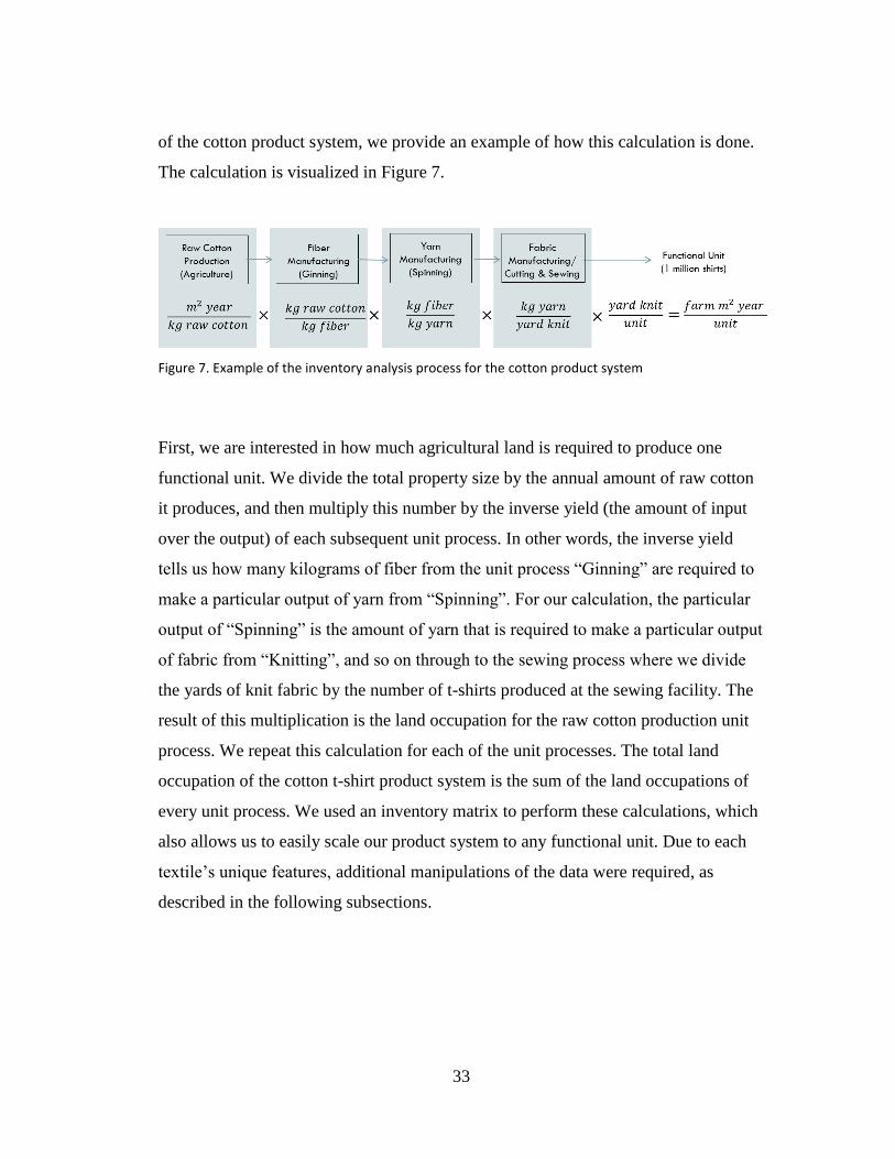
33
of the cotton product system, we provide an example of how this calculation is done.
The calculation is visualized in Figure 7.
Figure 7. Example of the inventory analysis process for the cotton product system
First, we are interested in how much agricultural land is required to produce one
functional unit. We divide the total property size by the annual amount of raw cotton
it produces, and then multiply this number by the inverse yield (the amount of input
over the output) of each subsequent unit process. In other words, the inverse yield
tells us how many kilograms of fiber from the unit process “Ginning” are required to
make a particular output of yarn from “Spinning”. For our calculation, the particular
output of “Spinning” is the amount of yarn that is required to make a particular output
of fabric from “Knitting”, and so on through to the sewing process where we divide
the yards of knit fabric by the number of t-shirts produced at the sewing facility. The
result of this multiplication is the land occupation for the raw cotton production unit
process. We repeat this calculation for each of the unit processes. The total land
occupation of the cotton t-shirt product system is the sum of the land occupations of
every unit process. We used an inventory matrix to perform these calculations, which
also allows us to easily scale our product system to any functional unit. Due to each
textile’s unique features, additional manipulations of the data were required, as
described in the following subsections.
34
Cotton
We were provided data for five cotton farms as a representative sample of the total
thirty farms supplying organic cotton for the studied t-shirt. We therefore averaged
the total size and total output, and thus yield, of these farms to be used for our
inventory calculation. All of these farms were found to be within the same ecoregion.
We have no reason to suspect that any one of these farms’ size, output, or yield is
more representative of the supplier’s typical farm, and thus we determined that an un-
weighted arithmetic mean was appropriate. Using the same reasoning, we also
averaged the land use and outputs of the two ginners used to produce this t-shirt.
Additionally, cotton farming produces burrs and cottonseed as economically valuable
co-products of fiber production; we therefore allocated the land occupation
accordingly. It was determined that an economic allocation would be more
appropriate than a mass-based allocation, because the disproportionate masses of the
co-products do not necessarily reflect the quantity of land being used for the unit
process. An economic allocation attributes the land used in the process based on the
product of interest’s portion of the profits derived from the process. Patagonia’s
cotton supplier estimated that cotton lint accounts for 80% of the profits of raw cotton,
thus we multiplied the land occupation by 80%. We then divided this by the total raw
cotton fiber produced. We did the same for the total ginning property, because
ginning is the process that separates the co-products.
Wool
Similar to cotton, Patagonia’s suppliers provided us with data on nine pastures, which
were reported to be representative of the forty-four pastures supplying the wool for
the studied t-shirt. Therefore, we determined that using the arithmetic mean of these
pastures’ land use and outputs was appropriate. Three mills in the same ecoregion are
used to perform the spinning process, so their land use and outputs were also
averaged. Wool also has an economically valuable co-product: mutton, or sheep meat.
The supplier estimated that 70% of the economic value derived from raising sheep is
35
from the wool fiber. The economic allocation factor was thus applied to the raw
material process by multiplying the total property size by 70% and dividing by the
total wool output.
Polyester
The raw material inputs required for the production of polyester polymer, petroleum
and natural gas, are commodity products, which means that location-specific data is
unavailable. To approximate this data, a model of the processes leading up to polymer
production was built in GaBi 6.0 (GaBi). GaBi is a professional software used widely
in life cycle assessment to model product systems. Databases such as Ecoinvent are
incorporated into GaBi to provide information collected from industry and science-
based research on the inputs and outputs of particular product systems. Therefore, we
were able to incorporate land occupation data from Ecoinvent with a model of the
polymer production unit processes to supplement the missing data.
The process ‘polyethylene terephthalate, granulate, amorphous, at plant’ (PET
amorphous) is used as the raw material for the polyester shirt. Any primary inputs
were retrieved from the Ecoinvent database and linked to this raw material process.
Using this Ecoinvent data, we determined that the unit processes for purified
terephthalic acid (PTA) and ethylene glycol (EG) are the two major sources of land
occupation flows. Using the Ecoinvent data, and the inventory calculation method
described above, we were able to determine approximately how much land
occupation the PTA and EG processes require to produce one functional unit.
Although the Ecoinvent database reports land occupation for 21 specific categories,
we excluded the categories of traffic area and water bodies, because these imply
incorporating more aspects of land occupation than were included for other unit
processes and textiles. We assigned the remaining 14 land occupation categories to
one of the four land use types used in our study (agriculture, urban, pasture, and
forest).

36
Lyocell
Calculating the impacts of lyocell was complicated by a few factors. First, the lyocell
t-shirt is 57% organic cotton and 43% lyocell by weight. We used the data gathered
for the organic cotton t-shirt to account for 57% of the fiber used to create the lyocell
t-shirt. As discussed further in our results and discussion section, based on our initial
findings for lyocell, we also completed calculations as though the shirt were made
from 100% lyocell. Unless otherwise noted, the results and discussion presented in
this paper refer to the 100% lyocell t-shirt. Second, the lyocell fiber is produced from
three types of trees—beech, spruce, and eucalyptus, each of which is grown in a
different region. Thus the raw material calculations had to be kept separate, and
incorporated proportionally to their contribution to the t-shirt into the inventory
calculation. The raw wood is pulped in three different countries—Austria, the Czech
Republic, and South Africa, while fiber processing is done in Austria, the United
Kingdom, and Alabama, so again the land occupation of the pulp and fiber had to be
incorporated proportionally.
Electricity
Because we did not have primary energy use data, secondary data from literature and
Ecoinvent were used to calculate results for electricity production. First, we used
existing literature (Lenzing Aktiengesellschaft 2012; van der Velden et al. 2013) to
determine how much electricity is used to produce a functional unit of each of the
fabrics in our study, or where possible to produce a particular output of each unit
process (e.g. 2.0 MJ electricity for raw fiber production per cotton t-shirt). Where a
range of values was provided, we choose to use the higher electricity consumption
data for our model. These values were limited to raw material production through
fabric manufacturing due to lack of available data for subsequent processes. We feel
it is reasonable to assume that later processes (finishing, cutting, and sewing) occupy
similar amounts of land for electricity generation across textiles, and that these
amounts will be small relative to the total land occupation of a particular textile.

37
Second, we selected electricity production processes from the Ecoinvent database to
obtain a list of the land occupation requirements in m2*years per MJ for each process.
Each of these land occupations was then multiplied by the values we found for MJ
per functional unit. Because production processes for most countries were unavailable
in Ecoinvent, we used US, electricity mix, agg, production mix for unit processes in
North and South America, China, electricity mix, agg, production mix for processes
in Asia, and RER, electricity mix, agg, production mix for processes in Europe. We
used the same process as for polyester raw materials to categorize the land occupation
data provided by Ecoinvent. Due to the uneven availability of electricity data and the
fact that electricity data were not provided in the same division of unit processes used
in this study (e.g. raw material production through spinning might be aggregated in
one number, or data for raw material production might be unavailable all together),
our reported results do not include electricity unless otherwise noted. Electricity
impacts as an example of background impacts were calculated separately and
evaluated in relation to the foreground impacts.
3.2 Characterization Factors
In their electronic supplementary material, de Baan et al. (2013b) provide a table of
their land occupation characterization factors. Each row contains the characterization
factors for a particular ecoregion; there is also a set of World Average
characterization factors. In each of the 867 ecoregions, there is one characterization
factor for every land use type (agriculture, pasture, managed forest, and urban) for
every taxonomic group (birds, mammals, reptiles, plants, and amphibians). There is
also an aggregated characterization factor for every land use type, which was
calculated based on a weighted average of all the characterization factors across
taxonomic groups. The weighting factor of median species richness per taxa
normalized by the median species richness of mammals was used to prevent plants,
which have many more species recorded than other taxa, from dominating the results.
We used this aggregated characterization factor to calculate our results, as overall

38
species loss as opposed to species loss per taxa was our interest. We used the
characterization factor table to assign a characterization factor to each unit process
based on its ecoregion and land use type. A sample of the characterization factors
used in this study is provided in Table 3.
Table 3. Examples of characterization factors used in this study. The unit for characterization factor is potentially lost non-endemic species for occupying one m
2 for one year
Characterization Factor
Ecoregion Land Use Type Unit Process
1.44x10⁻¹⁰
West shortlands grass Agriculture Cotton raw production
1.04x10⁻⁹
Southern Asia: Thailand Urban Wool knitting
2.62x10⁻¹⁰
Southeastern mixed forests Urban Polyester fiber production
2.46x10⁻¹⁰
Cantabrian mixed forests Managed forest Lyocell tree production
5.56x10⁻¹¹
Western European broadleaf forests
Urban Lyocell tree pulping
3.2.1 Assigning Characterization Factors
It is important that inventory data be regionalized in the same manner as the
characterization factors being used (de Baan et al. 2013b). Thus, in order to apply the
characterization factors for measuring potential species extinction as done in our
study, inventory data had to be properly matched up with the appropriate land use
type, as well as the applicable regional classification, according to how the
characterization factors were developed.
In order to determine the ecoregion in which the unit process takes place, the facility
locations were converted to latitude and longitude coordinates, and overlaid onto the
ecoregion map created by Olson et al. Because characterization factors are provided
for four broad land use types, we assigned each unit process a land use type based on
general knowledge (e.g. cotton farming is agriculture, wool grazing is pasture, and
spinning is urban). Using the published table of regional biodiversity characterization

39
factors (de Baan et al. 2013b) we then determined the characterization factor
associated with that ecoregion and land use type. World average characterization
factors were used for the polyester raw material and all background electricity
calculations, because specific locations for these processes were unknown.
3.2.2 Adapting Characterization Factors
Because our final impact calculation requires one characterization factor, we had to
create an adapted characterization factor for unit processes for which the ecoregion
was unknown (e.g. we were provided with the source country, rather than an address)
or which take place in multiple ecoregions. Characterization factors had to be adapted
for the raw inputs of lyocell and wool.
Lyocell
For eucalyptus, beech, and spruce wood used in lyocell production, the supplier
provided the source countries for each wood type, rather than a specific facility
address. Each of these countries contains multiple ecoregions, and since ecoregions
span political borders, it was necessary to aggregate the characterization factors
accordingly. Specifically, beech and spruce are harvested from managed forests
across central Europe, including the countries of Austria, the Czech Republic,
Slovakia, Germany, Hungary, France, Belgium, Romania, Ukraine, Croatia, Bosnia,
Slovenia, Belarus, and Switzerland. Eucalyptus is grown on plantations in eastern
South African provinces and Swaziland, where it is a non-native species. Because the
supplier, SAPPI, also produces pulp, paper, and chemical cellulose, it is impossible to
identify the specific plantations providing the eucalyptus pulp used to produce the
studied lyocell. A weighted characterization factor was created for each wood type
based on the quantity of that wood sourced from each country listed as a supplier, as
well as the portion of the beech-, spruce-, or eucalyptus-supplying ecoregion falling
within those countries.
40
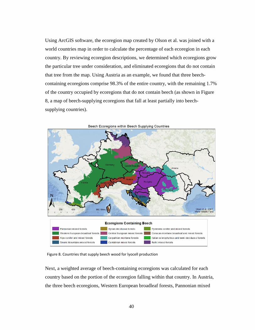
Using ArcGIS software, the ecoregion map created by Olson et al. was joined with a
world countries map in order to calculate the percentage of each ecoregion in each
country. By reviewing ecoregion descriptions, we determined which ecoregions grow
the particular tree under consideration, and eliminated ecoregions that do not contain
that tree from the map. Using Austria as an example, we found that three beech-
containing ecoregions comprise 98.3% of the entire country, with the remaining 1.7%
of the country occupied by ecoregions that do not contain beech (as shown in Figure
8, a map of beech-supplying ecoregions that fall at least partially into beech-
supplying countries).
Figure 8. Countries that supply beech wood for lyocell production
Next, a weighted average of beech-containing ecoregions was calculated for each
country based on the portion of the ecoregion falling within that country. In Austria,
the three beech ecoregions, Western European broadleaf forests, Pannonian mixed
41
forests, and Alps conifer and mixed forests, make up 21.1%, 18.9%, and 58.3% of
Austria’s area, respectively. To account for the 1.7% of the country that does not
grow any beech, we divided each of the aforementioned ecoregion percentages by
0.983 to find the portion of each beech-supplying ecoregion in the area of Austrian
beech-growing ecoregions. Thus the make up of the potential beech-supplying area of
Austria is 21.5% Western European broadleaf forests, 19.2% Pannonian mixed
forests, and 59.3% Alps conifer and mixed forests. Each ecoregion’s characterization
factor was multiplied by its respective contribution to the beech growing area of
Austria, and the results were summed to calculate a weighted characterization factor
for Austria’s beech harvesting. This weighted characterization factor was then
multiplied by 50%, since 50% of beech used in lyocell production is sourced from
Austria. This process was repeated to find a country-specific characterization factor
for the other countries that supply beech. All country adapted characterization factors
were added together according to the percentage of total beech they supplied,
resulting in a single adapted characterization factor for the entire beech production
unit process. Finally, these adapted country-specific characterization factors were
used to find a single characterization factor for the entire production of each wood
type, using a weighted average based on the percent contribution of that country to
lyocell production. The same steps were repeated to develop a single characterization
factor for the production of spruce.
For eucalyptus, the regions of Mpumalanga and KwaZulu Natal in South Africa and
the entirety of Swaziland were given as locations for eucalyptus plantations. Any
ecoregions falling at least partially within those areas were identified and included in
a GIS map (Figure 9), with the exception of ecoregions in which eucalyptus
plantations would be infeasible, such as mangroves. An average characterization
factor was created for the remaining ecoregions, weighted based on the relative size
of each ecoregion within the country.

42
Figure 9. Countries and ecoregions that supply eucalyptus for lyocell production
Figure 10. Countries and ecoregions that supply wool
Wool
The wool used in the studied wool t-shirt is sourced from 44 pastures spread across
southern Argentina. Representative data was provided for nine of these pastures,
which are distributed across four ecoregions. Therefore, it was necessary to create a
single, representative characterization factor from the unique characterization factors
that corresponded to the four ecoregions supplying wool. The location of the pastures
and the corresponding ecoregions can be seen in Figure 10. After identifying the
characterization factors associated with each of the nine pastures, an average
characterization factor was created, using a non-weighted arithmetic mean, to
represent all forty-four source pastures.

43
3.3 Impact Assessment
In order to calculate regional impacts from land occupation, for each unit process, the
land occupation inventory result (measured in m2*years per functional unit) is
multiplied by the characterization factor corresponding to the location and land use
type of that unit process. The result is a biodiversity impact measured in potentially
lost non-endemic species per functional unit. The total biodiversity impact is
calculated for each unit process as shown in Equation 1,
Eq. 1
where BIk is the biodiversity impact of unit process k; LOk is the land occupation in
m2*years per functional unit for unit process k; and CFi,j is the characterization factor
for land use type i in ecoregion j. To calculate the total impact of the textile across the
product system, the biodiversity impacts (BI) are summed (Equation 2).
∑ Eq. 2
Calculating the background impacts and polyester raw material impacts we use the
same basic equation, but use different subscripts (Equation 3),
∑ Eq. 3
where BIn is the biodiversity impact of land occupation of one of the fourteen
Ecoinvent land occupation categories; LOn is the land use occupation of category n;
and CFi,w is the world average characterization factor of the land use type of category
i. Summing up the land use impact of all categories gives us the total background
impact, or total polyester raw material impact. Background impacts can be summed
with foreground impacts to get a total impact.
44
3.4 Scenario Analysis
After analyzing our initial results, we conducted scenario analyses to better
understand the key drivers of our results and the effect of our assumptions. Because
agricultural and pastoral unit processes proved to be significant contributors to total
biodiversity impacts and total land occupation, we analyzed the effect of changing
variables affecting those results, as described in the following subsections.
3.4.1 Hypothetical Change of Raw Material Source Location
For both cotton and wool we calculated a biodiversity impact of the t-shirt system
based on a realistic change in the raw material sourcing location. Patagonia also
sources wool from Australia, and primarily sources cotton from regions around
Indore and Akola, India. For both scenarios, we were given broad regional sourcing
locations, and thus had to create a single adapted characterization factor as was done
for lyocell, described in Section 3.2.2. For wool, we used a straight average of the
characterization factors for ecoregions which were likely to contain wool grazing
operations, determined using the “Gridded Livestock of the World” (GLW), a
distribution map of sheep and other livestock developed by FAO’s Animal
Production and Health Division in collaboration with the Environmental Research
Group Oxford (FAO 2014). Similarly for cotton, ecoregions did not coincide directly
with the Indian Provinces, and therefore characterization factors for the ecoregions
present within sourcing provinces were averaged to produce a single characterization
factor. In both scenarios, land occupation and data for processes subsequent to wool
and cotton production were held the same as our original calculations, and a total
biodiversity impact was calculated using our original method for both textiles.
3.4.2 Impact of Wool Sourcing Assumptions
Patagonia’s suppliers provided us with data on only nine Ovis XXI pastures, which
we were told were representative of all forty-four Ovis XXI operations. We assumed
“representative” to include all aspects of the pastures including location and yield, as
well as the contribution of each operation to Patagonia’s wool t-shirt. In order to

45
assess how this assumption might have affected our results, we recalculated our
biodiversity impact for the entire product system nine times, each time using the raw
material data from only one pasture. In this way, we were able to identify the lowest
and highest impact operations, and provide a range for the possible impacts of the
wool product system to reflect possible differences in distribution of pasture yield and
location. We also took a straight average of the impacts generated by the nine farms
when assessed individually, and evaluated how the results of this average differed
from our initial results, in which we averaged yield and characterization factor rather
than impact.

46
4 Results
4.1 Cotton
The results of our cotton inventory analysis and impact assessment are shown in
Table 4. All characterization factors shown are the median, aggregated
characterization factors for the particular land use type and ecoregion of the unit
process. The total land occupation of the cotton t-shirt is 1.59x10⁷ m
2*years per
functional unit. The total biodiversity impact of the cotton t-shirt is 2.29x10⁻³
potentially lost non-endemic species per functional unit. Nearly 100% of both the
total land occupation and total impact of the cotton t-shirt comes from the raw
material production unit process. The regional characterization factor for the spinning
process is zero, because it is calculated using a local characterization factor for a
desert biome where the dominant land use type, pasture, leads to potential species
benefits. De Baan et al. (2013b) capped beneficial values at zero, thus the median
species loss was assumed to be zero. As a result, the total biodiversity impact of
spinning is also zero. As explained in Section 3.1.4 the displayed results for cotton,
and the three subsequent textiles report foreground impacts only.
4.2 Wool
Table 5 shows that the total land occupation calculated in our wool inventory analysis
is 1.77x10⁹ m
2*years per functional unit; the total biodiversity impact for the wool t-
shirt is 4.75x10⁻²
potentially lost non-endemic species per functional unit. As in
cotton, the characterization factors shown are the median, aggregated characterization
factors. The raw material process contributes more than 99% of both the total land
occupation and total biodiversity impact of the wool t-shirt.

47
4.3 Polyester
Table 6 displays the results of the polyester inventory analysis and impact assessment.
Land occupation of the polyester t-shirt is 1.92x10⁴
m2*years per functional unit, and
the biodiversity impact is 5.02x10⁻⁶
potentially lost non-endemic species per
functional unit. A characterization factor for raw material production is not displayed,
because as described in Section 3.1.4, world average characterization factors were
combined with land occupation data from the Ecoinvent database to calculate the
biodiversity impact. Unlike the other studied textiles, polyester’s land use processes
are all classified as urban land use types. Land occupation and biodiversity impacts of
all unit processes are distributed fairly evenly, with the exception of spinning and
finishing. Spinning contributes less than 5% of both total land occupation and total
biodiversity impact; finishing contributes 3.06% and 8.11% respectively.
4.4 Lyocell
Cotton production in the cotton-lyocell blended t-shirt accounts for 94% of the total
biodiversity impact, although it accounts for only half of the blended fiber by weight.
Therefore, in order to look more closely at the impacts from beech, spruce, and
eucalyptus, we conducted our analysis based on the results (Table 7) of modeling a
100% lyocell t-shirt. In doing so, we find that beech and eucalyptus are the two
greatest contributors to both the t-shirt’s total land occupation (9.77x10⁵ m
2*years per
functional unit) and total biodiversity impact (3.02x10⁻⁴
potentially lost non-endemic
species per functional unit). Beech production contributes 68% of the total land
occupation, but only 11% of the total biodiversity impact of the 100% lyocell t-shirt;
eucalyptus production accounts for 30% of land occupation and 81% of the
biodiversity impact. The characterization factor for eucalyptus production, which uses
plantations and is thus classified as agriculture, is approximately 17 times greater than
the characterization factor for beech, which is harvested from managed forests. The
cutting and sewing unit process contributes an additional 7.5% to total biodiversity
impact.

48
Table 4. Results of cotton inventory analysis (land occupation measured in m2*years per functional unit) and impact assessment (biodiversity impact
measured in potentially lost non-endemic species per functional unit)
Cotton Production Fiber Production Spinning Knitting/ Sewing Total
Land Occupation 1.59x10⁷ 1.00x10³ 1.82x10² 4.72x10³ 1.59x10⁷
Percent of Total 99.96% 0.01% 0.00% 0.03%
Character. Factor 1.44x10⁻¹⁰ 7.65x10⁻¹¹ 0.00 4.86x10⁻¹⁰
Biodiversity Impact 2.28x10⁻³ 7.67x10⁻⁸ 0.00 2.29x10⁻⁶ 2.29x10⁻³
Percent of Total 99.90% 0.00% 0.00% 0.10%
Table 5. Results of wool inventory analysis (land occupation measured in m2*years per functional unit) and impact assessment (biodiversity impact measured in potentially lost non-endemic species per functional unit)
Raw Wool Production Fiber Production Spinning Knitting/ Finish Cutting/ Sewing Total
Land Occupation 1.77x10⁹ 2.85x10³ 1.09x10³ 4.39x10⁵ 1.55x10³ 1.77x10⁹
Percent of Total 99.97% 0.00% 0.00% 0.02% 0.00%
Character. Factor 2.66x10⁻¹¹ 2.38x10⁻¹¹ 1.13x10⁻¹⁰ 1.04x10⁻⁹ 1.67x10⁻¹⁰
Biodiversity Impact 4.71x10⁻² 6.77x10⁻⁸ 1.23x10⁻⁷ 4.58x10⁻⁴ 2.59x10⁻⁷ 4.75x10⁻²
Percent of Total 99.04% 0.00% 0.00% 0.96% 0.00%
Table 6. Results of polyester inventory analysis (land occupation measured in m2*years per functional unit) and impact assessment (biodiversity measured in potentially lost non-endemic species per functional unit)
Polymer Production Fiber Production Spinning Finishing Cutting Sewing Total
Land Occupation 7.53x10³ 3.56x10³ 8.38x10² 5.88x10² 2.63x10³ 4.07x10³ 1.92x10⁴
Percent of Total 39.20% 18.51% 4.36% 3.06% 13.69% 21.18% Character. Factor --- 2.62E-10 1.14E-10 6.93E-10 4.17E-10 4.17E-10
Biodiversity Impact 7.95x10⁻⁷ 9.31x10⁻⁷ 9.51x10⁻⁸ 4.07x10⁻⁷ 1.10x10⁻⁶ 1.70x10⁻⁶ 5.02x10⁻⁶
Percent of Total 15.83% 18.54% 1.89% 8.11% 21.83% 33.78%

49
Table 7. Results of lyocell inventory analysis (land occupation measured in m2*years per functional unit) and impact assessment (biodiversity measured in potentially lost non-endemic species per functional unit). Results from top continue into bottom table
Raw Material Production Pulping Fiber Production
Beech Spruce Eucalyptus Beech Spruce Eucalyptus Austria U.K. U.S.
Land Occupation 6.62x10⁵ 1.86x10³ 2.90x10⁵ 3.12x10² 2.24x101 1.80x10² 2.19x10³ 3.16x10² 2.06Ex103 Percent of Total 67.76% 0.19% 29.67% 0.03% 0.00% 0.02% 0.22% 0.03% 0.21%
Character. Factor 5.01x10⁻¹¹ 6.48x10⁻¹¹ 8.40x10⁻¹⁰ 5.56x10⁻¹¹ 2.30x10⁻¹¹ 4.56x10⁻⁹ 5.56x10⁻¹¹ 1.20x10⁻¹¹ 7.37x10⁻¹¹
Biodiversity Impact 3.32x10⁻⁵ 1.20x10⁻⁷ 2.43x10⁻⁴ 1.73x10⁻⁸ 5.13x10⁻¹⁰ 8.22x10⁻⁷ 1.22x10⁻⁷ 3.79x10⁻⁹ 1.52x10⁻⁷ Percent of Total 11.00% 0.04% 80.68% 0.01% 0.00% 0.27% 0.04% 0.00% 0.05%
Table continued from above Spinning Knitting Finishing Cutting/ Sewing Total
Land Occupation 1.23x10³ 6.40x10³ 9.96x10² 9.56x10³ 9.77x10⁵ Percent of Total 0.13% 0.66% 0.10% 0.98%
Character. Factor 3.16x10⁻¹⁰ 1.39x10⁻¹⁰ 1.39x10⁻¹⁰ 2.35x10⁻⁹
Biodiversity Impact 3.87x10⁻⁷ 8.88x10⁻⁷ 1.38x10⁻⁷ 2.24x10⁻⁵ 3.02x10⁻⁴ Percent of Total 0.13% 0.29% 0.05% 7.44%

50
4.5 Background Impacts
As shown in Table 8, electricity production accounts for than less 1% of the total combined
foreground plus background biodiversity impact for all textiles except polyester when calculated
using a world average characterization factor. In polyester, electricity accounts for almost 75%
of the total biodiversity impact. Land occupation ranges from 2.15x10⁴
for cotton to 1.5x10⁵ for
polyester. Total biodiversity impact of electricity production ranges from 2.07x10⁻⁶
for cotton to
1.46x10⁻⁵
for polyester.
Table 8. Total land occupation and total biodiversity impact of electricity production for each t-shirt (land occupation in m
2* years per functional unit; biodiversity impact in potentially lost non-endemic species per
functional unit). The bottom row displays the contribution of electricity’s biodiversity impact to the total combined (foreground processes plus electricity) biodiversity impact of the product system
Cotton Wool Lyocell Polyester
Land Occupation for Electricity Production
2.15x10⁴ 4.62x10⁴ 2.57x10⁴ 1.5x10⁵
Biodiversity Impact of Electricity Production
2.07x10⁻⁶ 4.38x10⁻⁶ 2.39x10⁻⁶ 1.46x10⁻⁵
Foreground Biodiversity Impact 2.29x10⁻³ 4.75x10⁻² 3.02x10⁻⁴ 5.02x10⁻⁶
Contribution to Combined Foreground + Background Biodiversity Impact
0.09% 0.01% 0.79% 74.45%
4.6 Uncertainty Analysis
It is important to note in considering these results that de Baan et al. found high uncertainty when
using Monte Carlo simulations to propagate parameter uncertainty into the characterization
factors used in this study (de Baan et al. 2013b). De Baan et al. calculated characterization
factors for the upper and lower bound of a 95% confidence interval (referred to within as High
CF and Low CF, respectively), which we used to calculate the high and low biodiversity impacts
of every unit process for each t-shirt. The results are shown Tables 7a, b, c, and d. For each unit
process we calculated a high and low biodiversity impact value from the upper and lower bound
characterization factors published by de Baan et al. (2013b), and then calculated the percent
change of these new values from the biodiversity impact calculated using the median value
characterization factor (reported in Sections 4.1-4.5).

51
In cotton, using high and low characterization factors, we found a 227% increase and a 186%
decrease, respectively, in total biodiversity impact (Table 7a). The greatest change was a 1001%
decrease in the biodiversity impact of the knitting and sewing unit process using the low
characterization factor; the smallest change was a 185% decrease in the raw material production
impact. As described in Section 4.1, values could not be calculated for spinning yarn unit process
of the cotton t-shirt. For wool, the high characterization factor produced an increase in total
biodiversity impact of 188%, while using the low characterization factor decreased the
biodiversity impact of the t-shirt by 131% (Table 7b). The percent change using a high or low
characterization factor ranged from 123% decrease (raw material production) to a 1907%
increase (spinning), with the biggest changes occurring in spinning and fiber production. The
total biodiversity impact for the polyester t-shirt increases by 959% using the upper bound
confidence interval characterization factor and decreases 1353% using the low characterization
factor (Table 7c). For the lyocell material, the total biodiversity impact increases by 240%, using
the upper bound characterization factor, and decreases by 203% using the lower bound
characterization factor. There was a large range in the percent change from using the high and
low bound of the characterization factors. The range was between a 197% change and a 3888%
change, which occurred in the lyocell fiber production process in the UK facility. Using the
lower bound characterization factor for this facility decreased the biodiversity impact by two
orders of magnitude (Table 7d).
The vast range across the textiles of percent change in biodiversity impact resulting from using
either a high or low characterization factor is due to the equally large differences between the
biodiversity impacts of the materials. Because polyester has a relatively small biodiversity
impact, a change in the characterization factor due to uncertainty is going to be felt much more
strongly than a change to the characterization factor for wool, which is miniscule relative to its
land occupation.

52
Table 9a-9d. CF = characterization factor. Impact refers to biodiversity impact in potentially lost non-endemic species per functional unit. Median to High or Low % Change refers to the percent change of the biodiversity impact as calculated using the median CF versus the high or low 95% confidence interval CF
Table 9a. Results of cotton uncertainty analysis
Cotton Production Fiber Production Spinning Knitting/ Sewing Total
Median CF 1.44x10⁻¹⁰
7.65x10⁻¹¹
0 4.86x10⁻¹⁰
Median Impact 2.28x10⁻³
7.67x10⁻⁸
0 2.29x10⁻⁶
2.29x10⁻³
High CF 4.70x10⁻¹⁰
5.07x10⁻¹⁰
3.05x10⁻⁸
3.35x10⁻⁹
High Impact 7.45x10⁻³
5.08x10⁻⁷
5.55x10⁻⁶
1.58x10⁻⁵
7.47x10⁻³
Med. to High % Change 226% 563% --- 590% 227%
Low CF -1.22x10⁻¹⁰
-5.39x10⁻¹⁰
-1.51x10⁻⁸
-4.38x10⁻⁹
Low Impact -1.93x10⁻³
-5.41x10⁻⁷
-2.74x10⁻⁶
-2.06x10⁻⁵
-1.95x10⁻³
Med. to Low % Change -185% -805% --- -1001% -186%
Table 9b. Results of wool uncertainty analysis
Wool Material Fiber Production Spinning Knitting/ Finish Cutting/ Sewing Total
Median CF 2.66x10⁻¹¹
2.38x10⁻¹¹
1.13x10⁻¹⁰
1.04x10⁻⁹
1.67x10⁻¹⁰
Median Impact 4.71x10⁻²
6.77x10⁻⁸
1.23x10⁻⁷
4.58x10⁻⁴
2.59x10⁻⁷
4.75x10⁻²
High CF 7.58x10⁻¹¹
1.87x10⁻¹⁰
1.27x10⁻⁹
6.07x10⁻⁹
9.59x10⁻¹⁰
High Impact 1.34x10⁻¹
5.33x10⁻⁷
1.38x10⁻⁶
2.66x10⁻³
1.48x10⁻⁶
1.37x10⁻¹
Med. to High % Change 185% 688% 1023% 481% 474% 188%
Low CF -6.12x10⁻¹²
-2.45x10⁻¹⁰
-2.04x10⁻⁹
-8.46x10⁻⁹
-1.24x10⁻⁹
Low Impact -1.08x10⁻²
-6.97x10⁻⁷
-2.23x10⁻⁶
-3.71x10⁻³
-1.91x10⁻⁶
-1.45x10⁻²
Med. to Low % Change -123% -1130% -1907% -910% -839% -131%
Table 9c. Results of polyester uncertainty analysis
Polymer Production Fiber Production Spinning Finishing Cutting Sewing Total
Median CF --- 2.62x10⁻¹⁰
1.14x10⁻¹⁰
6.93x10⁻¹⁰
4.17x10⁻¹⁰
4.17x10⁻¹⁰
Median Impact 7.95x10⁻⁷
9.31x10⁻⁷
9.51x10⁻⁸
4.07x10-07
1.10x10⁻⁶
1.70x10⁻⁶
5.02x10⁻⁶
High CF 1.24x10⁻⁹
1.97x10⁻⁹
1.17x10⁻⁹
3.14x10-09
5.08x10⁻⁹
5.08x10⁻⁹
High Impact 9.33x10⁻⁶
6.99x10⁻⁶
9.83x10⁻⁷
1.85x10-06
1.34x10⁻⁵
2.07x10⁻⁵
5.32x10⁻⁵
Med. to High % Change 1073% 651% 933% 353% 1119% 1119% 959%
Low CF -1.22x10⁻⁹
-1.49x10⁻⁹
-1.29x10⁻⁹
-1.24x10⁻⁹
-6.96x10⁻⁹
-6.96x10⁻⁹
Low Impact -9.21x10⁻⁶
-5.32x10⁻⁶
-1.08x10⁻⁶
-7.27x10⁻⁷
-1.83x10⁻⁵
-2.83x10⁻⁵
-6.29x10⁻⁵
Med. to Low % Change -1259% -671% -1236% -278% -1769% -1769% -1353%

53
Table 9d. Results of 100% lyocell uncertainty analysis (results continue in table below)
Raw Material Production Pulping Fiber Production
Beech Spruce Eucalyptus Beech Spruce Eucalyptus Austria U.K. U.S.
Median CF 5.01×10⁻¹¹
6.48×10⁻¹¹
8.40×10⁻¹⁰
5.56×10⁻¹¹
2.30×10⁻¹¹
4.56×10⁻⁹
5.56×10⁻¹¹
1.20×10⁻¹¹
7.37×10⁻¹¹
Median Impact 3.32×10⁻⁵
1.20×10⁻⁶
2.43×10⁻⁴
1.73×10⁻⁸
5.13×10⁻¹⁰
8.22×10⁻⁷
1.22×10⁻⁷
3.79×10⁻⁹
1.52×10⁻⁷
High CF 7.15×10⁻¹⁰
7.02×10⁻¹⁰
2.50×10⁻⁹
3.99×10⁻¹⁰
2.67×10⁻¹⁰
2.66×10⁻⁸
3.99×10⁻¹⁰
3.69×10⁻¹⁰
1.09×10⁻⁹
High Impact 4.74×10⁻⁴
1.31×10⁻⁶
7.24×10⁻⁶
1.24×10⁻⁷
5.97×10⁻⁹
4.80×10⁻⁶
8.75×10⁻⁷
1.17×10⁻⁷
2.25×10⁻⁶
Med. to High % Change
1327% 983% 197% 618% 1064% 483% 618% 2984% 1380%
Low CF -4.29×10⁻¹⁰
-4.56×10⁻¹⁰
-8.25×10⁻¹⁰
-7.10×10⁻¹⁰
-4.19×10⁻¹⁰
-3.67×10⁻¹⁰
-7.10×10⁻¹⁰
-4.53×10⁻¹⁰
-7.90×10⁻¹⁰
Low Impact -2.84×10⁻⁴
-8.49×10⁻⁷
-2.39×10⁻⁴
-2.21×10⁻⁷
-9.37×10⁻⁹
-6.62×10⁻⁶
-1.56×10⁻⁶
-1.43×10⁻⁷
-1.63×10⁻⁶
Med. to Low % Change
-956% -804% -198% -1378% -1927% -905% -1378% -3888% -1172%
Table continued from above
Spinning Knitting Finishing Cutting/ Sewing Total
Median CF 3.16×10⁻¹¹
1.39×10⁻¹¹
1.39×10⁻¹¹
2.35×10⁻¹¹
Median Impact 3.87×10-07
8.88×10-07
1.38×10-07
2.24×10-05
3.02×10-04
High CF 2.00×10-09
1.01×10-09
1.01×10-09
2.72×10-08
High Impact 2.45×10-06
6.47×10-06
1.01×10-06
2.60×10-04
1.48×10-03
Median to High % Change
532% 629% 629% 1057% 389%
Low CF -2.83×10⁻¹⁰
-1.73×10⁻¹⁰
-1.73×10-09
-3.31×10-08
Low Impact -3.47×10-06
-1.11×10-05
-1.73×10-06
-3.16×10-04
-8.67×10-04
Median to Low % Change
-995% -1348% -1348% -1510% -387%
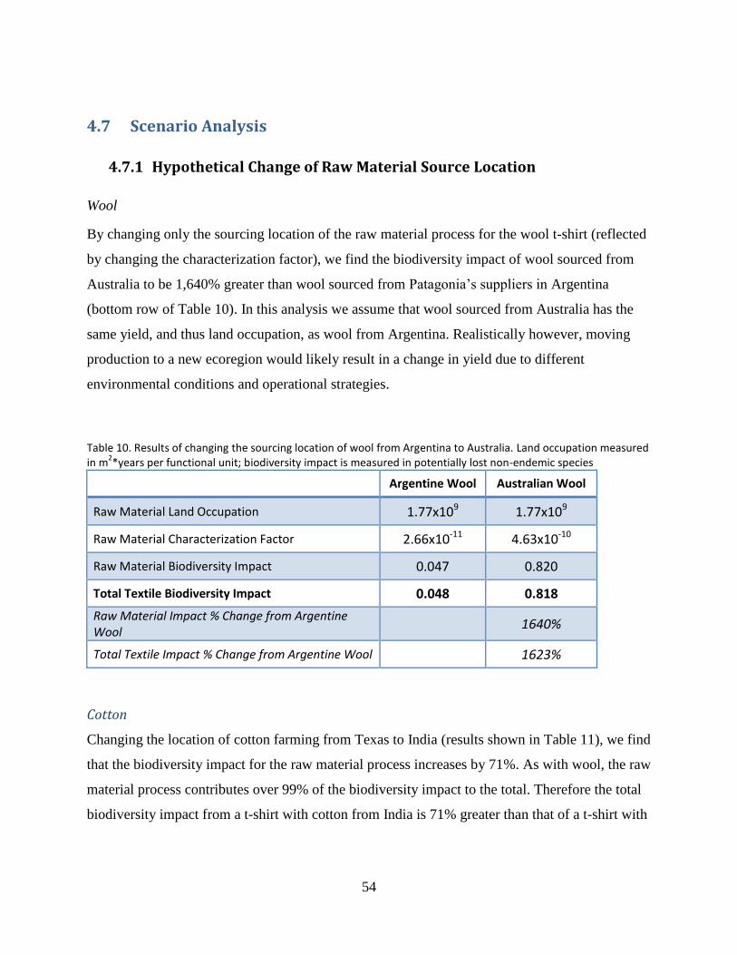
54
4.7 Scenario Analysis
4.7.1 Hypothetical Change of Raw Material Source Location
Wool
By changing only the sourcing location of the raw material process for the wool t-shirt (reflected
by changing the characterization factor), we find the biodiversity impact of wool sourced from
Australia to be 1,640% greater than wool sourced from Patagonia’s suppliers in Argentina
(bottom row of Table 10). In this analysis we assume that wool sourced from Australia has the
same yield, and thus land occupation, as wool from Argentina. Realistically however, moving
production to a new ecoregion would likely result in a change in yield due to different
environmental conditions and operational strategies.
Table 10. Results of changing the sourcing location of wool from Argentina to Australia. Land occupation measured in m
2*years per functional unit; biodiversity impact is measured in potentially lost non-endemic species
Argentine Wool Australian Wool
Raw Material Land Occupation 1.77x10⁹ 1.77x10⁹
Raw Material Characterization Factor 2.66x10⁻¹¹ 4.63x10⁻¹⁰
Raw Material Biodiversity Impact 0.047 0.820
Total Textile Biodiversity Impact 0.048 0.818
Raw Material Impact % Change from Argentine Wool
1640%
Total Textile Impact % Change from Argentine Wool 1623%
Cotton
Changing the location of cotton farming from Texas to India (results shown in Table 11), we find
that the biodiversity impact for the raw material process increases by 71%. As with wool, the raw
material process contributes over 99% of the biodiversity impact to the total. Therefore the total
biodiversity impact from a t-shirt with cotton from India is 71% greater than that of a t-shirt with

55
cotton produced in Texas. As with wool, we assume the yield of a cotton farm is the same in
India as in Texas, though in reality they may be different.
Table 11. Results of changing the sourcing location of cotton from Texas to India. Land occupation measured in m
2*years per functional unit; biodiversity impact is measured in potentially lost non-endemic species
Texas Cotton Indian Cotton
Raw Material Land Occupation 1.59x10⁷ 1.59x10⁷
Raw Material Characterization Factor 1.44x10⁻¹⁰ 2.47x10⁻¹⁰
Raw Material Biodiversity Impact 2.28x10⁻³ 3.91x10⁻³
Total Textile Biodiversity Impact 2.29x10⁻³ 3.92x10⁻³
Raw Material Impact % Change from Texas cotton
71%
Total Textile Impact % Change from Texas cotton
71%
4.7.2 Testing Assumptions of Raw Wool Impact Assessment
The wool supplier provided data on nine grazing operations, which were labeled as
“representative” of the forty-four total pastures that provide wool for this t-shirt. In the original
impact assessment we assumed “representative” to be inclusive of yield and location distribution,
and contribution of wool to Patagonia’s t-shirt. We thus used a straight average of the size,
output, and characterization factor of each operation, essentially creating one unit process with a
yield and characterization factor equivalent to the averages of those nine operations.
In order to test this assumption, we calculated the biodiversity impact per functional unit of the
wool t-shirt for each of the nine grazing operations, as though the wool were sourced entirely
from that grazing operation. Shown in Table 12, El Cronometro has the lowest operational
impact while La Isabel has the highest operational impact in units of potentially lost non-
endemic species per functional unit. We find that if the wool were sourced entirely from the
operation with the highest impact, El Cronometro, the total biodiversity impact of 1 million wool
t-shirts would increase by 258% to 0.17 potentially lost non-endemic species; if it were sourced
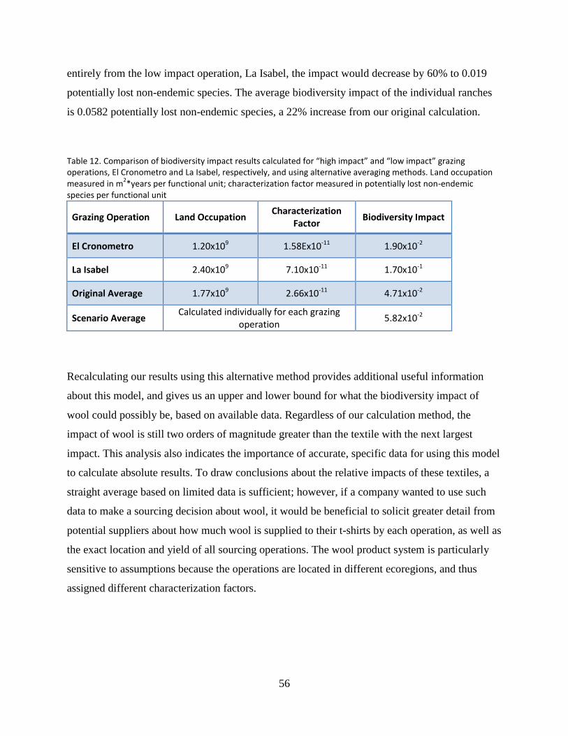
56
entirely from the low impact operation, La Isabel, the impact would decrease by 60% to 0.019
potentially lost non-endemic species. The average biodiversity impact of the individual ranches
is 0.0582 potentially lost non-endemic species, a 22% increase from our original calculation.
Table 12. Comparison of biodiversity impact results calculated for “high impact” and “low impact” grazing operations, El Cronometro and La Isabel, respectively, and using alternative averaging methods. Land occupation measured in m
2*years per functional unit; characterization factor measured in potentially lost non-endemic
species per functional unit
Recalculating our results using this alternative method provides additional useful information
about this model, and gives us an upper and lower bound for what the biodiversity impact of
wool could possibly be, based on available data. Regardless of our calculation method, the
impact of wool is still two orders of magnitude greater than the textile with the next largest
impact. This analysis also indicates the importance of accurate, specific data for using this model
to calculate absolute results. To draw conclusions about the relative impacts of these textiles, a
straight average based on limited data is sufficient; however, if a company wanted to use such
data to make a sourcing decision about wool, it would be beneficial to solicit greater detail from
potential suppliers about how much wool is supplied to their t-shirts by each operation, as well as
the exact location and yield of all sourcing operations. The wool product system is particularly
sensitive to assumptions because the operations are located in different ecoregions, and thus
assigned different characterization factors.
Grazing Operation Land Occupation Characterization
Factor Biodiversity Impact
El Cronometro 1.20x10⁹ 1.58Ex10-11 1.90x10⁻²
La Isabel 2.40x10⁹ 7.10x10⁻¹¹ 1.70x10⁻¹
Original Average 1.77x10⁹ 2.66x10⁻¹¹ 4.71x10⁻²
Scenario Average Calculated individually for each grazing
operation 5.82x10⁻²

57
5 Discussion
5.1 Wide Range of Biodiversity Impacts and Land Occupation
We find that the biodiversity impacts and land occupation of the four textiles are separated by
orders of magnitude. Taking our results at face value, we find that the production of one million
wool t-shirts leads to the potential loss of roughly 4.8% of a non-endemic species regionally,
while all other textiles produce a loss of less than 1%. The total biodiversity impact of wool is 21
times greater than cotton, 157 times greater than lyocell, and more than 9,000 times greater than
polyester, as shown in the bottom row of Table 13. Total land occupation for the four textiles is
similarly distributed, spanning nearly 5 acres for polyester to over 437,000 acres in the case of
wool, ultimately responsible for the wide range of total biodiversity impacts among the four
textiles. The sheer magnitude of land occupation required for agriculture and pasture dwarfs the
influence of location and land use type as captured by the characterization factor.
Table 13. Total land occupation (m
2*years per functional unit) and biodiversity impact (potentially lost non-
endemic species per functional unit) per textile and ratio of each textile to wool, the textile with the greatest biodiversity impact
Wool Cotton Lyocell Polyester
Total Land Occupation 1.77x10⁹ 1.5x10⁷ 9.77x10⁵ 1.92x10⁴
Biodiversity Impact 0.04751 0.00229 0.00030 0.00001
Ratio Textile to Wool 1:1 1:21 1:157 1:9461
While this range of values is interesting, three important points should be made. First, from the
perspective of our client, other apparel companies, and their customers, these four textiles serve
different functions and are not necessarily exchangeable. Therefore, looking across materials
may not be particularly useful to a company making decisions about its products—while
Patagonia would like to minimize the impact of its cotton t-shirts, and could thus compare two
cotton product systems, it would not replace its cotton shirts with polyester, because the two
textiles serve different purposes. Second, biodiversity loss is only one of many environmental
impacts to which t-shirt production contributes, and a textile with a low impact to biodiversity
58
loss from its land use may have a large impact with regards to greenhouse gas emissions, water
requirements, or other impacts. Third, the broad classification scheme used in this model likely
overestimates the biodiversity impact of wool (as well as other materials potentially), while the
high uncertainty of the characterization factors is carried over into our results. The wool supplied
for this t-shirt is sourced from a 40 million acre restoration effort between Ovis XXI, The Nature
Conservancy, and the Savory Institute, which is intended to restore biodiversity by using a land
management strategy that reverses the desertification of native grasslands due to human
mismanagement of livestock (Savory Institute 2012). Sheep are moved between pastures, rather
than grazing continuously on one plot of land, which reduces pressure on the landscape.
However, because the assessed model uses only four broad land use types, classifying wool
production as “pasture” does not capture the sustainable grazing strategies used by the t-shirt’s
wool suppliers.
5.2 Importance of Raw Material Production
Raw material production contributes more than 99% of the total biodiversity impact of the cotton
and wool t-shirts, and 94% of the total biodiversity impact of the lyocell t-shirt. For polyester,
which is produced using entirely urban classified land use types, this contribution is only 16%.
This high contribution of the raw material process is due to the low yield, and thus large land
occupation, of the agriculture, pasture, and managed forest land use types required for producing
cotton, wool, and tree pulp relative to the minimal land occupation required for all subsequent,
urban-based manufacturing processes.
5.3 Influence of the Characterization Factors
Although raw material land occupation dominates the total biodiversity impact for the cotton,
wool, and lyocell t-shirts, location and land use type as captured by the characterization factors
do influence outcomes. The role of the characterization factor in relative biodiversity impact can
be seen particularly in lyocell raw material production, throughout the polyester product system,
and in our scenario analysis of wool raw material production. Although the land use type plays a
role in determining the characterization factor, companies using this model will have a limited
ability to change the land use type associated with product production. Lyocell is an example of

59
a product for which a company does have some control over land use type, as cellulose could be
sourced from either managed forests or plantations (classified as agriculture).
Lyocell
Looking more closely at the dominant lyocell unit processes (eucalyptus and beech production),
we find that although beech makes up only 38% (by weight) of the pulp mix used for Patagonia’s
lyocell, it contributes 68% of the total land occupation, which indicates that beech requires more
land per ton dry output. In fact, beech requires about 3.5 times more land than eucalyptus to
produce the same weight of dry output (shown in Table 14). However, we find that these higher
land requirements are offset by the characterization factors.
Table 14. Comparison of biodiversity impact in potentially lost non-endemic species for producing one oven-dried ton of beech or eucalyptus, and corresponding characterization factors in potentially lost non-endemic species for occupying 1 m
2 for 1 year. CF=characterization factor
Beech Production Eucalyptus
Production (Actual)
Eucalyptus
Production
(Modified)
Land use type of CF used Managed Forest Agriculture Managed Forest
Annual yield (odt/m2) 0.00034 0.00120 0.00120
Land occupation (m2/odt) 2,940 833 833
Characterization factor 5.01x10⁻¹¹ 8.40x10⁻¹⁰ 3.72x10⁻¹⁰
Biodiversity impact 1.47x10⁻¹¹ 7.00x10⁻¹¹ 3.10x10⁻¹¹
Because the eucalyptus used in Patagonia’s lyocell is harvested from plantations, it is classified
as an agricultural land use, while beech is considered managed forest; eucalyptus is sourced from
South Africa, and beech is sourced from Central Europe. If land occupation alone were driving
the biodiversity impact, we would expect beech to have a correspondingly higher impact than
eucalyptus. Instead, our results indicate that the biodiversity impact of eucalyptus per oven dried
ton is 4.75 times greater than that of beech (Table 14). To understand whether this discrepancy
arises from the land use type or the location component of the characterization factor, we
compared the impact eucalyptus production would have if classified as managed forest instead of
agriculture. Changing the land use type of the characterization factor for eucalyptus, but
60
maintaining its same ecoregion, we found that the impact was still 2.26 times greater than that of
beech (Table 14). This implies that the more intensive agricultural land use of eucalyptus, in
addition to its more sensitive sourcing region, is influencing the biodiversity impact. Modifying
the land use type without changing the location or yield is purely hypothetical, as in practice
plantation tree farming is going to have a higher yield than a managed forest, and eucalyptus
may not be harvested from managed forests in South Africa.
Polyester
As shown in Figure 11, the total land occupation and total biodiversity impact of polyester are
distributed much more evenly across the unit processes, all of which are classified as an urban
land use type, unlike the other textiles which require agriculture and pasture. If the
characterization factors did not influence biodiversity impact, we would expect the two series in
Figure 11 (contribution of the unit process to total biodiversity impact and contribution of the
unit process to land occupation) to follow the same pattern. However, we see that while the raw
material process is the largest contributor to land occupation, it is only the fourth largest
contributor to total biodiversity impact. Additionally, although finishing is the smallest
contributor to land occupation, spinning is the smallest contributor to biodiversity impact. These
changes indicate that the process locations, as contained in the characterization factor, influence
polyester’s biodiversity impact. Unlike the other textiles for which raw material land occupation
is so large, and thus dominant in the biodiversity impact results, polyester’s land occupation is
relatively small, so the characterization factor exerts an influence on biodiversity impact.

61
Figure 11. Percent contribution of land occupation and biodiversity impact of each unit process to the total biodiversity impact (potentially lost non-endemic species per functional unit) and land occupation (m2*years)
5.4 Contribution of Electricity Impacts
As reported in Table 8 in Section 4.5, electricity contributes less than 1% to the total combined
foreground plus background biodiversity impacts of cotton, wool, and lyocell, yet in polyester it
accounts for nearly 75%. Although the land occupation required for polyester electricity
production and resulting biodiversity impact are an order of magnitude larger than the other
materials, the relatively high contribution of electricity is due to the fact that polyester’s
foreground biodiversity impact is orders of magnitude smaller than the other textiles’ impacts.
As mentioned previously, biodiversity impacts of land occupation for electricity production are
included in this case study as an example of how the model can be used to evaluate and
incorporate background processes. We find that a lack of primary data on electricity
consumption per unit process and location of occupation for electricity generation, as well as the
fact that Ecoinvent provides only country-wide electricity production mix data, reduces the
accuracy and meaningfulness of these results. These data gaps mean that the same world average
median urban characterization factor was used to calculate the results for all unit processes for all
four textiles; and that production mixes for the U.S., China, and Europe were broadly used to
calculate land occupation requirements for each unit process. This additionally means that

62
energy consumption per functional unit, which was drawn from literature, was the primary
variable differentiating our results. In practice, companies are likely to be able to gain access to
energy consumption data, but may have a more difficult time identifying the location where
electricity is generated, and will likely need to rely on countrywide Ecoinvent land occupation
data. For the calculated biodiversity impact of electricity generation to be more accurate and
meaningful, electricity consumption data should be gathered directly from the supplier and a
general location of electricity generation is needed; increased availability of regionally specific
data in Ecoinvent would also be useful.

63
6 Limitations & Conclusions
The primary objective of our study was to explore the robustness of an emerging model for
incorporating land use impacts on biodiversity into LCA. Through our results and analysis we
identify four key limitations to using the model as it exists, which prevent it from being ready to
incorporate operationally alongside other environmental indicators in LCA. Although with
refinement and increased data availability, the model has potential for future use, it is currently
better suited for providing broad generalizations about land occupation impacts on biodiversity
than for specific use in decision making or for conducting refined product system assessments.
6.1 Limitation 1: High characterization factor uncertainty
The first limitation of using the model is the high level of uncertainty in the resulting
characterization factors. As explained by de Baan et al. (2013b) in their report, the sensitivity
parameter, or relative decrease in species richness, used to calculate the characterization factors
contributed between 67% and 96% of the variance. This uncertainty is due to a lack of taxa- and
ecoregion-specific data, which required that some values be aggregated across larger spatial units
than ecoregions, such as biomes or the globe (de Baan et al. 2013b). Taking uncertainty into
account, all of our unit process biodiversity impact values range from the land occupation having
a detrimental effect (a positive biodiversity impact) to a beneficial effect on biodiversity (a
negative biodiversity impact), as does each total product system (shown in Figure 12).
Figure 12. Range of total biodiversity impact per textile as calculated using the high (dark blue), median (green) and low (light blue) characterization factors of a 95% confidence interval. Biodiversity impact is shown in thousandths of a potentially lost non-endemic species per functional unit
64
For cotton, wool, and lyocell the majority of this range falls within the positive domain,
indicating a detriment to biodiversity; for polyester the majority actually falls in the negative
domain, indicating a biodiversity benefit. This uncertainty limits the confidence with which
conclusions can be drawn from these results, and with which our findings could be used for
decision-making. In effect we find that wool t-shirt production might lead to the greatest
biodiversity loss, or it might produce the greatest gain. Still, under both high and low uncertainty
scenarios, raw material unit processes remain the greatest contributors to total impact for cotton,
wool, and lyocell; wool continues to have the greatest impact, whether beneficial or detrimental,
of the four textiles.
6.2 Limitation 2: Cannot capture nuances in land use types
The second significant limitation is that the characterization factors consider only four broad
land use types, even though land is used in myriad ways. This broad classification scheme means
that the model cannot distinguish between finer land cover types such as crop type, vineyard, or
orchard within agriculture, or high and low intensity industrial or residential land uses within the
urban classification. Similarly, land use management strategies, such as organic and conventional
farming or sustainable versus traditional grazing cannot be differentiated. In addition to the wool
example provided in Section 6.1, the cotton used in the assessed t-shirt is made from 100%
organic cotton. The extensive nature (i.e. lower yield, higher land occupation) of organic farming
is often cited as being less ecologically damaging compared to more intensive conventional
farming practices, because the management technique allows the physical and biological
processes of the land to continue functioning. Yet this potential benefit cannot be captured using
the characterization factors applied in this study; a high-yield cotton farm will always show a
lower impact result as compared to a low-yield cotton farm in the same ecoregion. For a
company like Patagonia seeking the most sustainable options, and committed to sourcing 100%
organic cotton, it is important to be able to distinguish between land use management techniques
when making sourcing decisions.

65
Consensus is also lacking among the multitude of existing global land use and land cover maps
(de Baan et al. 2013b). Harmonizing and updating global land cover maps to include
management regimes and fine land use types is an enormous effort, but one that may be
necessary for these characterization factors to be used effectively. Refinement of the
characterization factors to align with these narrower land classifications will increase the
resolution of the information provided by such impact assessments. Although some research
proposes a classification scheme using more than 75 land use types (Koellner et al. 2013a), it is
more difficult to generate a refined database of characterization factors for such detailed land
classifications, representing a significant trade-off if used in the currently available
characterization factor model.
6.3 Limitation 3: Need for location-specific data
Third, to use this database of characterization factors meaningfully requires knowledge of the
locations where facilities or processes occur. For many companies, particularly those lacking
transparency in their supply chain, heavily reliant on commodity products, or sourcing materials
from a multitude of locations, this information may be difficult or impossible to obtain, and
regional accuracy will not be possible in the results. Although a world average characterization
factor can be used to supplement this data, this adds a further layer of uncertainty to the results.
6.4 Limitation 4: Captures limited aspects of biodiversity
Finally, to reiterate Section 2.3 of this report, biodiversity is complex and this model captures
only limited aspects of it. The calculation of biodiversity loss or extinction potential in this
model is based on the species area relationship (SAR) model, as well as the sensitivity of species
to land use change, which is based on species richness. These two measures of biodiversity loss
do not capture the many other aspects of biodiversity, which are considered to be equally
important for healthy environmental conditions. Genetic diversity, or the diversity within a
species is critical to the long-term survival of a species, but this aspect is currently not captured.
Ecosystem diversity is also not incorporated and therefore leaves out the consideration of many
different types of habitat, which can support a distinct variety of species. The relative abundance
of species is also not captured and each species is weighted equally, therefore species with a
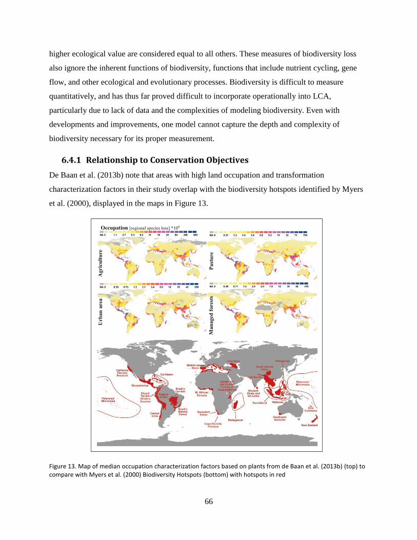
66
higher ecological value are considered equal to all others. These measures of biodiversity loss
also ignore the inherent functions of biodiversity, functions that include nutrient cycling, gene
flow, and other ecological and evolutionary processes. Biodiversity is difficult to measure
quantitatively, and has thus far proved difficult to incorporate operationally into LCA,
particularly due to lack of data and the complexities of modeling biodiversity. Even with
developments and improvements, one model cannot capture the depth and complexity of
biodiversity necessary for its proper measurement.
6.4.1 Relationship to Conservation Objectives
De Baan et al. (2013b) note that areas with high land occupation and transformation
characterization factors in their study overlap with the biodiversity hotspots identified by Myers
et al. (2000), displayed in the maps in Figure 13.
Figure 13. Map of median occupation characterization factors based on plants from de Baan et al. (2013b) (top) to compare with Myers et al. (2000) Biodiversity Hotspots (bottom) with hotspots in red
67
Biodiversity hotspots are defined as areas that have both high concentrations of endemic species,
and that are experiencing an unusually high rate of habitat depletion (Myers 1998).
The darker areas of the de Baan et al. (2013b) map (top) correspond with biodiversity hotspots
shown in red on the Myers et al. (2000) map (bottom). Although biodiversity hotspots have been
suggested by some as a means to set conservation priorities, and biodiversity hotspots may be an
important indicator of previous land use conversion, they may not always meet desired
conservation goals as resources are inevitably too scant for protecting all threatened and
endangered species. Brooks et al. (2006) identify biodiversity hotspots as a reactive global
conservation priority, distinct from proactive priorities in that the focus is on areas of high
vulnerability (such as those with which high characterization factors are associated) rather than
areas of low vulnerability (such as those with which low characterization factors are associated).
Large, undisturbed areas are considered low-vulnerability; yet provide great potential for
conservation. Depending on whether the objective of the user is to conserve prime biodiversity
habitat for the future or to conserve already heavily degraded land, the conservation strategy will
change. De Baan et al. (2013b) recognize that their characterization factors are intended to assess
impacts reactively, or retrospectively, as they look specifically at historical, average land use
changes. Thus de Baan et al. used land use scenarios for 2050 to calculate prospective
characterization factors, though this was done for only 19 ecoregions of the Amazon. They found
that characterization factors changed most notably in ecoregions with large projected
deforestation rates (de Baan et al. 2013b). As developments in the data and methods progress,
the prospective approach suggested and briefly tested by de Baan et al. (2013b) for calculating
the potential future loss of species through marginal land use changes may be more applicable in
situations where there is a large portion of undisturbed land that faces serious future land use
threats (de Baan et al. 2013b). The important point to be drawn is that propagating one set of
characterization factors, such as those developed by de Baan et al., throughout an industry or
LCA implicitly assigns value to certain facets of biodiversity and conservation priorities, while
neglecting others which may be equally important and relevant.

68
6.5 Limitations of the Case Study
In addition to the limitations of the characterization factor, which are inherently carried into our
case study, a limitation of our case study is that we did not model transformation or permanent
impacts. In order to measure total global biodiversity impacts, occupation, transformation, and
permanent impacts must all be summed. This is necessary since occupation and transformation
impacts assess reversible regional extinctions whereas permanent impacts measure irreversible,
permanent extinctions based on endemic species. Thus, the results of our study indicate only
reversible extinction risk rather than permanent extinction of endemic species.

69
7 Recommendations
7.1 Recommendations for the Model
De Baan et al. (2013b) recognize that a number of factors limit the applicability of their regional
characterization factors, and accordingly outline recommendations for improvements and future
research. Generally increasing the quantity, diversity, and resolution of data on species and land
use will lead to improved characterization factors, including those reviewed in this study for land
occupation. In particular, de Baan et al. recommend:
1. Adding new species data to the WWF database from which biodiversity and global land
use data are drawn. This will produce more accurate characterization factors. In particular,
increasing data on taxonomic groups currently underrepresented in research, such as
reptiles and amphibians, would be useful in improving the characterization factors.
2. “Better data on taxa- and eco-region specific habitat suitability for different land use
types (de Baan et al. 2013b)” will improve the certainty of the model by reducing the
need to aggregate input parameters across broader spatial units than ecoregions.
Increasing the detail, accuracy, and agreement between global land use classification
maps could also reduce uncertainty.
Although any improvement in data robustness will subsequently improve the applicability of this
model, it will still be limited by the high uncertainty that arises from the intricate nature of
biodiversity, particularly as it relates to fitting within an LCA framework. Measuring only one
aspect of biodiversity, such as species richness, leaves out the many other aspects that could be
considered such as genetic diversity, functional diversity, structural diversity, and spatial
distribution. Therefore, even with increased data on species richness at a high-resolution spatial
scale, many aspects of biodiversity would be omitted, which limit the potential for this model as
tool to be used on its own. With regards to application within the apparel industry, and perhaps
in corporate sustainability decision-making generally, our greatest recommendation for the
development of future models is to prioritize the incorporation of a highly defined land use
classification scheme. Although data availability is currently an obstacle, when it comes to

70
product sourcing, company’s need to be able to identify the benefits of one land use management
strategy over another, in addition to differences arising from land occupation and location. When
deciding to source 100% organic cotton, for example, a company should be able to quantify the
impacts of that decision on biodiversity alongside its affect on water consumption,
environmental toxicity, and global warming.
7.2 Recommendations for Patagonia
Although the limitations of the model prevent us from recommending that it be used
operationally alongside other LCA indicators, the model as applied through this study reveals
important information regarding land use impacts on biodiversity. A review of the results does
provide interesting insight into Patagonia’s product systems and the complexities of trying to
quantify biodiversity, which can help guide future sourcing decisions, even though we cannot
recommend relying firmly on the numbers provided by this model. Our analysis leads us to the
following recommendations for Patagonia and other companies looking to evaluate their
biodiversity impact from land use.
Agricultural and pastoral land uses contribute significantly to the overall biodiversity impact of a
t-shirt due to their large land requirements per output, signifying that Patagonia, as well as other
apparel companies using agriculture or grazing, may not need to look beyond total land
occupation to approximate their biodiversity impacts. Relying on the results of this model would
indicate that increasing yields from these processes is one way to reduce the per-unit biodiversity
impact of a product system. However, increasing yields is typically tied to more intensive land
use, which may put greater pressure on a particular ecosystem, and require inputs of fertilizer,
pesticides, and water, among others. Moving to a higher-yield management strategy (e.g.
conventional cotton farming from organic) may simply shift land occupation impacts to other
environmental categories. For example, the burden of impacts could shift to water pollution, or
affect different aspects of biodiversity such as microbial diversity, in turn degrading soil fertility.
As an alternative, we recommend that Patagonia look qualitatively at the land use of its supply
chain, with a particular focus on identifying methods for improving agricultural and pastoral
processes. As a part of this qualitative assessment, it would be beneficial to fully understand the
land management strategies used by suppliers, and to research the benefits or negative impacts of

71
particular land management practices such as organic farming and holistic land management on
biodiversity to inform sourcing decisions. To decrease impacts associated with processes
producing the raw materials, such as cotton, wool, and timber, Patagonia should continue to
develop partnerships with organizations like The Nature Conservancy and suppliers like Ovis
XXI. Working with these groups, Patagonia can support the use of innovative sustainable land
management strategies. Patagonia can also continue to work closely with their suppliers to
minimize inputs that may have harmful effects on biodiversity, whether in their production or
use phase. While these impacts on biodiversity may not result from land use directly, they may
be the result of the other harmful inputs to the environment. Decreasing water use, chemical use,
water pollution, and fertilizer may all help to minimize impacts on biodiversity. Patagonia has
little capability to decrease the land use associated with urban processes such as sewing, spinning,
or knitting. Instead, Patagonia could look into conservation and biodiversity offset options to
lessen the impacts resulting from their urban land uses, such as forest restoration, natural habitat
preservation, or habitat remediation.
Although this model does not yet provide the granularity necessary for us to recommend its use
widely within apparel life cycle assessments, primarily due to its inability to distinguish between
specific land use types, Patagonia and the Sustainable Apparel Coalition should continue their
pursuit of a methodology for quantifying biodiversity impacts. Biodiversity is critical for a
healthy future, and we cannot afford to neglect it in corporate decision-making. Pressure and
support from the apparel industry and others will help to drive the research necessary to develop
a robust model that allows companies to minimize impacts from land use on biodiversity.
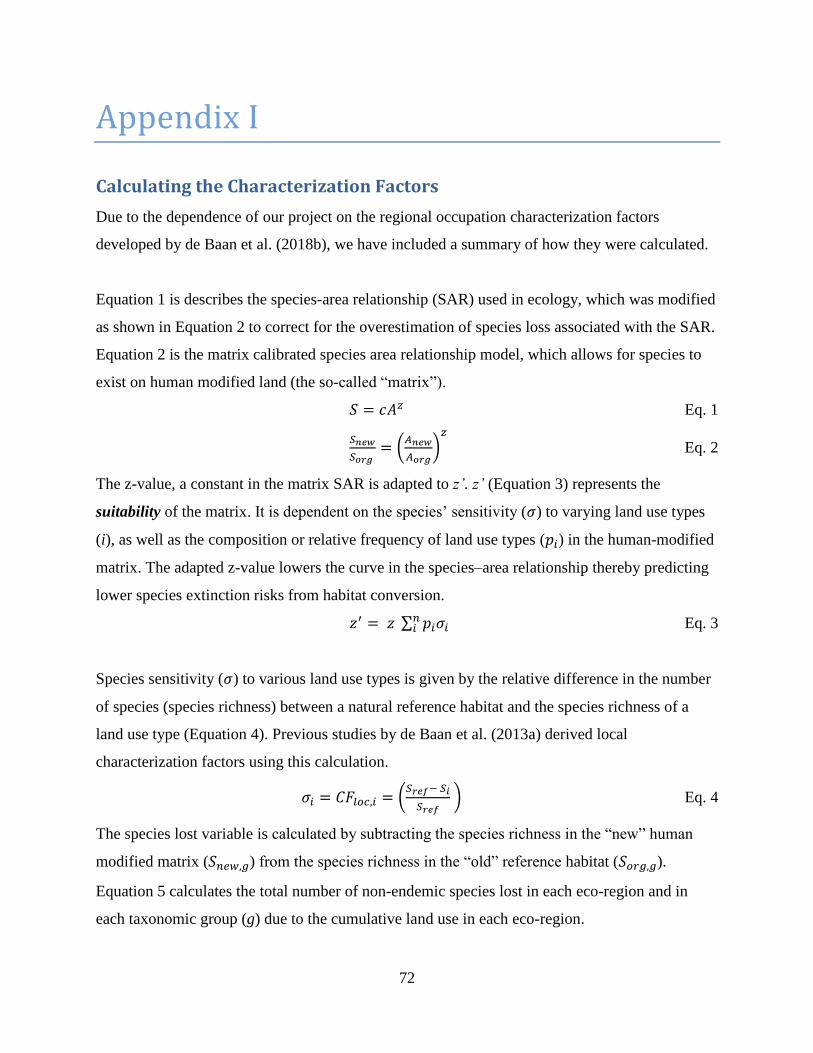
72
Appendix I
Calculating the Characterization Factors
Due to the dependence of our project on the regional occupation characterization factors
developed by de Baan et al. (2018b), we have included a summary of how they were calculated.
Equation 1 is describes the species-area relationship (SAR) used in ecology, which was modified
as shown in Equation 2 to correct for the overestimation of species loss associated with the SAR.
Equation 2 is the matrix calibrated species area relationship model, which allows for species to
exist on human modified land (the so-called “matrix”).
Eq. 1
(
)
Eq. 2
The z-value, a constant in the matrix SAR is adapted to z’. z’ (Equation 3) represents the
suitability of the matrix. It is dependent on the species’ sensitivity ( ) to varying land use types
(i), as well as the composition or relative frequency of land use types ( ) in the human-modified
matrix. The adapted z-value lowers the curve in the species–area relationship thereby predicting
lower species extinction risks from habitat conversion.
∑ Eq. 3
Species sensitivity ( ) to various land use types is given by the relative difference in the number
of species (species richness) between a natural reference habitat and the species richness of a
land use type (Equation 4). Previous studies by de Baan et al. (2013a) derived local
characterization factors using this calculation.
(
) Eq. 4
The species lost variable is calculated by subtracting the species richness in the “new” human
modified matrix ( ) from the species richness in the “old” reference habitat ( ).
Equation 5 calculates the total number of non-endemic species lost in each eco-region and in
each taxonomic group (g) due to the cumulative land use in each eco-region.

73
(
)
Eq. 5
The total non-endemic species lost in an ecoregion are then allocated to the differing land use
types, relative to their frequency. An allocation factor is calculated for each land use type i and
ecoregion j per Equation 6.
∑
Eq. 6
Characterization factors for occupation are calculated by combining the non-endemic species lost
per ecoregion and taxa variable, the allocation factor. Multiplying these factors results in non-
endemic species lost for specific land use types in each ecoregion based on the relative frequency
of a land use in the ecoregion. The species lost factors account for species’ differing sensitivities
to land use activities. The product of species lost and the allocation factor are divided by the area
occupied by a particular and use type i in a particular ecoregion j.
Characterization factors for occupation for each land use type and eco-region
Eq. 7

74
Appendix II
Supplier Questionnaire for Primary Data Collection
A similar questionnaire to the one provided here, adapted for the textile and unit process, was sent to
each supplier. A table was provided for suppliers to record their responses.
Please answer these questions to the best of your ability in the table provided on the page 2.
Please select several farms, which are representative of the farms that supply cotton to the Texas
Organic Cotton Marketing Cooperative.
If possible, please also provide a list of all farms, which produce cotton for the Texas Organic
Cotton Marketing Cooperative, including their locations and sizes, if possible. This can be
entered into the provided excel spreadsheet (email attachment). This information can also be
provided whatever way is most convenient for your party.
1. A. How many farms produce organic cotton for the TOCMC?
B. Identify the cotton farming operations by name or any other identification that are used to
produce cotton and are most representative of all the cotton supply farms in terms of size and
location?
1. What is the size of this property in hectares? If other units are used, please specify.
2. How many hectares are used for cotton production on this property?
3. What is the total amount (weight) of cotton that is produced on this farm annually?
4. What is the total amount (select unit) of cottonseed that is generated from this farm
annually?
5. How much cotton (weight) is acquired from this farm for Texas co-op annually?
6. Other than cottonseed, are there any other co-products of cotton production?
C. What is the location of these farming operations (address or coordinates)?
2. How long has this farm been on this land?
A. What length of time (years/months) has this cotton farming operation occupied this tract
of land?
B. Has the amount (hectares) of land used by this cotton farm increased over the past 20
years? Yes or No
If YES, what year did the size change to the current size (hectares)?
3. How is the land used at this cotton farming operation? Select a land use type from the list
provided at the end of the document.
4. Before this operation owned and operated this land, how was this land used? For historical
land use classification use the list provided at the end of the document.

75
Appendix III
Modeling Species Extinction: SAR vs. EAR
There are three popular models upon which species extinction estimates are based: the
Species-Area Relationship (SAR), the matrix-calibrated Species-Area Relationship, and the
Endemics-Area Relationship (EAR). Both the matrix modification of the SAR and the use of
the EAR aim to compensate for the overestimations of species extinction rates yielded from
tracing backwards along the traditional species-area curve of the SAR model (see backwards
SAR in Figure 14).
Figure 14. Estimating species extinctions due to habitat loss, from Rahbek, C. and R. K. Colwell (2011)
The traditional SAR model is based on island biogeography theory developed by MacArthur
and Wilson in the 1960s, and concludes that larger islands (habitat surrounded by unsuitable
habitat) contain more species than smaller islands. This model proposes that the number of
species on an island is a function of the immigration and extinction rates, relying on the
assumption that the population size of each species is proportional to the size of the island or
fragment (MacArthur and Wilson 1967). This species richness can be described by the power
relationship , in which S is the number of species in a habitat type of area A, and c
and z are constants. This relationship estimates the area required to sample the first individual

76
of a species. In order to calculate expected species lost, one can simply extrapolate backward
along the species-area curve.
The shortcomings of the SAR model that sparked introduction of the matrix-modified SAR
model include the assumption that: 1) land use between habitat areas being modeled,
otherwise known as the matrix, is inhospitable for species persistence, and 2) there are no
negative impacts of the matrix on habitat fragments. Since in reality, some species are able to
persist on human-modified land, a refinement of the SAR extinction approach was made by
adding terms to the power relationship that account for taxon-specific responses to individual
components of the matrix and edge effects (Koh & Ghazoul 2010; Koh et al. 2010). This
matrix-calibrated species area relationship curve effectively lowers the curve of the SAR (de
Baan et al. 2013b)
Despite improvements in the SAR approach made through the matrix-calibration, some
criticisms persist over estimating species loss based on either SAR or matrix-calibrated SAR.
For instance, if species of individuals are clumped, as is often the case in nature, then the area
added in order to find the first individual of a species is much smaller than the area that must
be removed to eliminate the last individual of the species. This species distribution factor is
the driver leading to overestimated extinction rate estimates. In other words, it takes a greater
loss of area to cause extinction of a species than it takes to find one, and this bias holds for
any power law species area function (SAR or matrix-calibrated). He and Hubbel (2011)
estimate that using the SAR potentially overestimates extinction rates by over 160%,
depending on the taxon and region.
Proposed by Harte and Kinzig (2000), the EAR is nearly opposite from the SAR, allowing for
the estimation of extinction based on the loss of habitat area by measuring the area required
to sample the last individual of a species, as opposed to the first. He and Hubbell (2011)
found both mathematically, and in examples using realistic spatial patterns of trees and birds,
that the backwards SAR curve always lies above the EAR curve (Figure 14), thus
overestimating expected extinction rates (Carsten & Colwell 2011).

77
References
Bartholomé, E., and A. S. Belward. "GLC2000: a new approach to global land cover mapping from Earth observation data." International Journal of Remote Sensing 26, no. 9 (2005): 1959-1977.
Biodiversity Hotspots Revisited, Conservation International, 2004. Conservation Synthesis,
Center for Applied Biodiversity Science at Conservation International. Online Linkages: http://www.biodiversityhotspots.org/xp/Hotspots/resources/maps.xml
Brooks, Thomas M., Russell A. Mittermeier, Gustavo AB da Fonseca, Justin Gerlach, Michael
Hoffmann, John F. Lamoreux, Cristina Goettsch Mittermeier, John D. Pilgrim, and ANDA SL Rodrigues. "Global biodiversity conservation priorities." science 313, no. 5783 (2006): 58-61.
Carpenter, Stephen R., Ruth De Fries, Thomas Dietz, Harold A. Mooney, Stephen Polasky, Walter
V. Reid, and Robert J. Scholes. "Millennium ecosystem assessment: research needs." (2006).
Davis, Mackenzie Leo, and David A. Cornwell. "Introduction to environmental engineering."
(2008). de Baan, Laura, Rob Alkemade, and Thomas Koellner. "Land use impacts on biodiversity in LCA: a
global approach." The International Journal of Life Cycle Assessment 18, no. 6 (2013): 1216-1230.
de Baan, Laura, Christopher L. Mutel, Michael Curran, Stefanie Hellweg, and Thomas Koellner.
"Land use in life cycle assessment: global characterization factors based on regional and global potential species extinction." Environmental science & technology 47, no. 16 (2013): 9281-9290.
Fischer, Joern, Berry Brosi, Gretchen C. Daily, Paul R. Ehrlich, Rebecca Goldman, Joshua Goldstein,
David B. Lindenmayer et al. "Should agricultural policies encourage land sparing or wildlife-friendly farming?." Frontiers in Ecology and the Environment 6, no. 7 (2008): 380-385.
Franklin, J. F. 1988. Structural and functional diversity in temperate forests. Pages 166-175 in E.O.
Wilson, editor. Biodiversity. National Academy Press, Washington, D.C. Ghazoul, Jaboury. "A Matrix‐Calibrated Species‐Area Model for Predicting Biodiversity Losses
Due to Land‐Use Change." Conservation Biology 24, no. 4 (2010): 994-1001. He, Fangliang, and Stephen P. Hubbell. "Species-area relationships always overestimate
extinction rates from habitat loss." Nature 473, no. 7347 (2011): 368-371. ISO, I. S. O. "14044: environmental management—life cycle assessment—requirements and
guidelines." International Organization for Standardization (2006).

78
Kareiva, Peter, and Michelle Marvier. "Conserving biodiversity coldspots." American Scientist 91, no. 4 (2003): 344-351.
Koellner, Thomas, Laura de Baan, Tabea Beck, Miguel Brandão, Barbara Civit, Mark Goedkoop,
Manuele Margni et al. "Principles for life cycle inventories of land use on a global scale." The International Journal of Life Cycle Assessment 18, no. 6 (2013): 1203-1215.
Koellner, Thomas, Laura de Baan, Tabea Beck, Miguel Brandão, Barbara Civit, Manuele Margni,
Llorenç Milà i Canals, Rosie Saad, Danielle Maia de Souza, and Ruedi Müller-Wenk. "UNEP-SETAC guideline on global land use impact assessment on biodiversity and ecosystem services in LCA." The International Journal of Life Cycle Assessment 18, no. 6 (2013): 1188-1202.
Koh, Lian Pin, Tien Ming Lee, Navjot S. Sodhi, and Jaboury Ghazoul. "An overhaul of the species–
area approach for predicting biodiversity loss: incorporating matrix and edge effects." Journal of applied ecology 47, no. 5 (2010): 1063-1070.
Lenzing Aktiengesellschaft. Focus Sustainability: Sustainability in the Lenzing Group. 2012.
http://www.lenzing.com/fileadmin/template/pdf/konzern/nachhaltigkeit/Sustainability_Report_2012_EN.pdf, accessed April 12, 2014.
MacArthur, Robert H. The theory of island biogeography. Vol. 1. Princeton University Press, 1967.
Margules, Chris R., and Robert L. Pressey. "Systematic conservation planning." Nature 405, no.
6783 (2000): 243-253.
Mittermeier, Russell A., Will R. Turner, Frank W. Larsen, Thomas M. Brooks, and Claude Gascon. "Global biodiversity conservation: the critical role of hotspots." In Biodiversity hotspots, pp. 3-22. Springer Berlin Heidelberg, 2011.
Mora, Camilo, Derek P. Tittensor, Sina Adl, Alastair GB Simpson, and Boris Worm. "How many
species are there on Earth and in the ocean?." PLoS biology 9, no. 8 (2011): e1001127. Myers, Norman, Russell A. Mittermeier, Cristina G. Mittermeier, Gustavo AB Da Fonseca, and
Jennifer Kent. "Biodiversity hotspots for conservation priorities." Nature 403, no. 6772 (2000): 853-858.
Myers, Norman. "Threatened biotas:" hot spots" in tropical forests." Environmentalist 8, no. 3
(1988): 187-208. Nachtergaele, Freddy. "Mapping land use systems at global and regional scales for land
degradation assessment analysis." (2010). United States. Congress. Office of Technology Assessment. Technologies to maintain biological
diversity. Vol. 330. DIANE Publishing, 1987. Olson, David M., Eric Dinerstein, Eric D. Wikramanayake, Neil D. Burgess, George VN Powell,
Emma C. Underwood, Jennifer A. D'amico et al. "Terrestrial Ecoregions of the World: A New Map of Life on Earth A new global map of terrestrial ecoregions provides an innovative tool for conserving biodiversity." BioScience 51, no. 11 (2001): 933-938.

79
Rahbek, Carsten, and Robert K. Colwell. "Biodiversity: Species loss revisited." Nature 473, no. 7347 (2011): 288-289.
Savory Institute. (2012). Savory Institute: Holistic Management Research Portfolio. Retrieved
from:http://www.savoryinstitute.com/media/40606/Savory_Inst_HM_Research_Portfolio_March2013.pdf
Stinner, Deborah H., Benjamin R. Stinner, and Edward Martsolf. "Biodiversity as an organizing
principle in agroecosystem management: case studies of holistic resource management practitioners in the USA." Agriculture, ecosystems & environment 62, no. 2 (1997): 199-213.
van der Velden, Natascha M., Martin K. Patel, and Joost G. Vogtländer. "LCA benchmarking study
on textiles made of cotton, polyester, nylon, acryl, or elastane." The International Journal of Life Cycle Assessment (2013): 1-26.
“WWF Ecoregion Descriptions,” World Wild Fund 2014, accessed March 15 2014.
http://worldwildlife.org/ecoregions/nt0402 World Countries (Generalized). (2010).SDC Feature Database. Digital Map. ESRI. ArcGIS Content
Team. “Wildfinder: Online database of species distributions, ver. Jan-06,” World Wildlife Fund 2006,
Accessed January 15 2014. https://worldwildlife.org/pages/wildfinder-database