Paper ID #19075

Incorporating Metrology Concepts into an Engineering Physics MeasurementsLaboratory

Dr. Harold T. Evensen, University of Wisconsin-Platteville

Hal Evensen is a earned his doctorate in Engineering Physics from the University of Wisconsin-Madison,where he performed research in the area of plasma nuclear fusion. He joined UW-Platteville in 1999, andformerly served as program coordinator for both its Engineering Physics and Microsystems & Nanoma-terials programs. He conducts research with students involving carbon nanotube electronics and sensors.

c©American Society for Engineering Education, 2017

Incorporating Metrology Concepts into an Engineering Physics Measurements Laboratory

We restructured an existing required, two-credit advanced laboratory course around the subject matter of metrology and design of experiments. Here, we present a significant extension from work that was presented in 2013. The course now uses international standards and terminology as set in documents from the Joint Committee for Guides in Metrology (JCGM) to guide students in the description and execution of experiments. Students learn to use appropriate vocabulary as defined in the International Vocabulary of Metrology (“VIM”) and handle uncertainty using the process described in the Guide to the expression of uncertainty in measurement (“GUM”). Students advance through a rotation of experiments that involve topics from mechanics, optics, electronics and quantum optics. The course follows a progressive structure by starting with conceptually simpler experiments designed to show the effects that the design of the experiment can have on the final result and its uncertainty. These early labs allow students to focus on concepts including Type A and Type B uncertainties; systematic errors; standard uncertainty and combined standard uncertainty; coverage factor; and the propagation of uncertainty. Students also begin to track uncertainty with a rudimentary uncertainty budget. For the rest of the course, the experiments become more open-ended and complex, and the students continue to apply the concepts learned in the first half of the semester. In this paper we will describe how focus on quality of measurement has affected students’ ability to design and analyze experiments, and will discuss plans for future improvement. Introduction The Engineering Physics (EP) program at the University of Wisconsin-Platteville includes a two-credit laboratory, “EP Lab,” that is typically taken in a student’s fifth semester. It is one of two courses that typically form a student’s first formal coursework in EP. As such, it is one of the first courses in which EP majors are not outnumbered by other majors and they can begin to form an “identity” as EP, which includes the ability to design and conduct open-ended, multidisciplinary experiments. (This course is similar to a “measurements lab” or “advanced” lab in other curricula.) We have been modifying the EP Lab with an enhanced focus on quality measurements and experiment design, and have incorporated topics from the field of Metrology to formalize this focus.1 Metrology, the science of measurement, is a core competency of STEM fields and plays a key role in modern engineering practice. More formally, metrology can be defined as the science of measurement and its application, including all theoretical and practical aspects of measurement, whatever the measurement uncertainty and field of application.2 There exists a large national and international community of engineers and scientists that work in the metrology field. Several aspects of metrology are now incorporated into EP Lab: (1) uncertainty in measurements (and its propagation); (2) use of metrology’s documented standard vocabulary and accepted practices; (3) using design of experiments (DOE) to analyze a process; (4) calibration of a measurement instrument or process.

The related learning objectives for EP Lab students are as follows (from the course syllabus):

Student Learning Objectives 1. Learn and correctly use the professional vocabulary of metrology and

measurement science associated with uncertainty & measurements; 2. Follow international standards in representation of uncertainty; 3. Assign uncertainty to a measurement by use of an uncertainty budget. This will

necessarily involve applying the following concepts: a. Identify Type A and Type B uncertainties; b. Calculate Type A uncertainties; c. Identify the proper probability distributions for Type B uncertainties; d. Calculate the combined standard uncertainty for a measurement; e. Calculate expanded uncertainty to give a confidence interval for a

measurement. 4. Assign uncertainty to the results of a calculation by using the mathematical model

of the measurement and the Law of Propagation of Uncertainty. 5. Understand and be able to explain the hierarchy of measurement standards.

Metrology: Vocabulary and Standard Procedures The vocabulary of metrology is contained in the International Vocabulary of Metrology (VIM),2

maintained by the Joint Committee for Guides in Metrology (JCGM).3 This 108-page, freely-available reference provides a standard vocabulary for measurement-related terms, and is a starting point to being conversant with others in the field. For this course, the VIM was distilled into three pages and 30terms; these are shown in Table 1 below. Table 1. The selection of VIM terms highlighted in EP Lab.

Metrology Measurement result Systematic error Measurement

uncertainty

Expanded measurement uncertainty

Quantity Metrological traceability

Repeatability condition

Type A evaluation Coverage factor

Measurand Influence quantity Repeatability Type B

evaluation Coverage

probability

Measurement principle Accuracy Reproducibility

condition

Instrumental measurement uncertainty

Uncertainty budget

Measurement method Precision Reproducibility

Standard measurement uncertainty

Measurement model

Measurement procedure Error Sensitivity

Combined standard

measurement uncertainty

Measurement function

These terms were used by the instructor throughout the semester, both verbally and in written experiment descriptions and handouts. Students were expected to apply these terms correctly in their reports. In addition, students completed an assignment in which they compared 12 of these terms using their own words. Learning and using the vocabulary also helped students navigate the experiments’ uncertainty analysis (below). The application of this vocabulary toward the mathematical treatment of uncertainty is described in another freely-available JCGM document: the “Guide to the expression of uncertainty in measurement” (GUM).4 The GUM focuses on the mathematical treatment of measurement uncertainty and “establishes general rules for evaluating and expressing uncertainty in measurement that are intended to be applicable to a broad spectrum of measurements.” It also establishes a philosophical approach to uncertainty by defining it as the “parameter, associated with the result of a measurement, that characterizes the dispersion of the values that could reasonably be attributed to the measurand.” (Emphasis added.) This is thus distinct from the common use of the term “error” as the difference between a measurement and its “true” value – which is unknowable in principle. As with the VIM, the GUM is rather extensive (134 pages). A portion of this document was extracted to create a reference handout for use in EP Lab. This handout summarizes the following topics using figures, examples, and language more appropriate for the educational setting:

• Type A (statistical) uncertainty; • Mean, standard deviation, and standard deviation of the mean; • Coverage interval and coverage probability; • Significant figures; • Type B uncertainty; • Application of the appropriate probability distribution function (rectangular, triangular,

U-shaped); • Incorporating manufacturer’s uncertainty specifications (expanded uncertainty); • Combined standard uncertainty; • Law of Propagation of Uncertainty; • Cosine error correction.

These concepts are applied to create an uncertainty budget, which is a table listing all components of a measurement’s uncertainty. For example, a measurement may have uncertainty contributions from resolution limits of an instrument, the manufacturer’s calibration/ specification, and the stability of the measurement. Creation of the budget causes students to consider all sources of uncertainty and to understand and apply the key topics listed above. While the uncertainty budget is not described in the GUM, it is a widely used tool to evaluate measurements; it is required for some ISO certifications.a The National Institute of Standards and Technology (NIST) has guidelines posted online.5 The uncertainty budget is useful because aSeeISO/IEC17025andA2LAlaboratoryaccreditationbodies.

(1) it identifies all sources of uncertainty and their relative magnitudes, allowing one to document a measurement’s precision and identify means to improve it; (2) it helps reduce mistakes in uncertainty calculations (or at least makes them easier to catch); (3) it can simplify and standardize uncertainty calculations. A screen shot of the modified uncertainty budget template used in this course is shown in Figure 1. (Students first created their own based on this template, then were provided the electronic file after the first two experiments.) Key aspects of an uncertainty budget include each source of uncertainty, plus: (1) uncertainty magnitudes; (2) units; (3) whether Type A or B; (4) applicable probability distribution function; (5) divisor (used to calculate standard uncertainty – can be an automated entry); (6) standard uncertainty. The table also shows the resultant combined standard uncertainty and can show the expanded uncertainty (i.e. the 90% confidence interval).

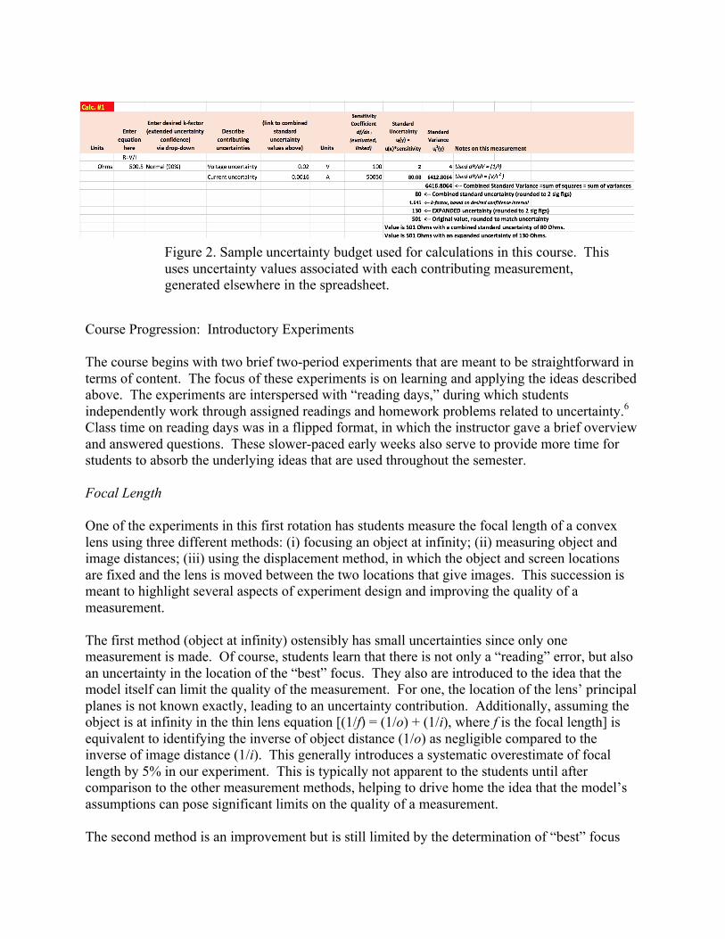
True uncertainty budgets also include the sensitivity and the degrees of freedom for each source, which were not included here. The “degrees of freedom” concept was left out of EP Lab for simplicity: its effect is typically mild and it was felt this concept would confuse the introduction desired here. Additionally, to help introduce this subject, the “sensitivity” was moved to a separate section of the uncertainty budget created by the instructor, described below. This second section of the uncertainty budget is dedicated to calculations involving the measured values; a segment is shown in Figure 2. The pedagogical intent was to keep the calculation of measurement uncertainty (i.e., Figure 1) distinct from the uncertainty of calculated values (i.e. Figure 2), as these concepts tend to get confused by the students. Having two separate sections also reduced “visual clutter” for the student, since sensitivity is typically exactly equal to one for each component of measurement uncertainty, and has other values only in the second section. The new “calculations” uncertainty budget of Figure 2 includes the calculated value and its equation, the desired expanded uncertainty, the contributing uncertainties (terms, magnitudes and units), the sensitivity to each term in the equation, and the standard uncertainties. It also displays the resultant combined standard uncertainty and expanded uncertainty.

Figure 1. Sample uncertainty budget used in this course. This is used to determine the combined standard uncertainty for a measurement. It has most of the features of a full uncertainty budget but lacks the degrees of freedom and sensitivity.

Course Progression: Introductory Experiments The course begins with two brief two-period experiments that are meant to be straightforward in terms of content. The focus of these experiments is on learning and applying the ideas described above. The experiments are interspersed with “reading days,” during which students independently work through assigned readings and homework problems related to uncertainty.6 Class time on reading days was in a flipped format, in which the instructor gave a brief overview and answered questions. These slower-paced early weeks also serve to provide more time for students to absorb the underlying ideas that are used throughout the semester. Focal Length One of the experiments in this first rotation has students measure the focal length of a convex lens using three different methods: (i) focusing an object at infinity; (ii) measuring object and image distances; (iii) using the displacement method, in which the object and screen locations are fixed and the lens is moved between the two locations that give images. This succession is meant to highlight several aspects of experiment design and improving the quality of a measurement. The first method (object at infinity) ostensibly has small uncertainties since only one measurement is made. Of course, students learn that there is not only a “reading” error, but also an uncertainty in the location of the “best” focus. They also are introduced to the idea that the model itself can limit the quality of the measurement. For one, the location of the lens’ principal planes is not known exactly, leading to an uncertainty contribution. Additionally, assuming the object is at infinity in the thin lens equation [(1/f) = (1/o) + (1/i), where f is the focal length] is equivalent to identifying the inverse of object distance (1/o) as negligible compared to the inverse of image distance (1/i). This generally introduces a systematic overestimate of focal length by 5% in our experiment. This is typically not apparent to the students until after comparison to the other measurement methods, helping to drive home the idea that the model’s assumptions can pose significant limits on the quality of a measurement. The second method is an improvement but is still limited by the determination of “best” focus

Figure 2. Sample uncertainty budget used for calculations in this course. This uses uncertainty values associated with each contributing measurement, generated elsewhere in the spreadsheet.

and the unknown location of the lens’ principal planes. Since more measurements are required, this experiment is used to introduce the uncertainty budget. The budget tracks the various sources of measurement uncertainty and their impact on the final, calculated value. Finally, the displacement method removes the problem of the unknown principal plane. Depending on the students’ ability to determine the best focus, this method may be said to give the best results. Students report on the results of all three models, identify and support their best determination of focal length, and comment on the accuracy, precision, etc. of the measurement, thus reinforcing the vocabulary. With the simple physics and procedure, students could form insights on the model limitations, the “best” experiment, and how a measurement may be improved. Since the students were left to determine the best way to conduct the experiment, it should be noted that the results typically varied depending on their assumptions – and procedural errors. It should also be noted that since virtually no students have taken the advanced Optics course at this point, there is no attempt to deal with topics such as the wavelength dependence of focal length or lens aberrations. Internal Resistance of a Multimeter The other experiment in this first rotation has students measure the internal resistance of a Fluke 117 Multimeter, using a calibrated voltage source (5V ± 0.01%)7 and an external resistor. Students are provided the circuit shown in Figure 3 and told to derive the expression for the internal resistance based on the external resistance, calibrated source voltage, and voltage displayed by the meter. Students have typically had Circuits I by this point, so this is trivial – once they have grasped the concept of internal resistance.

Students are provided three resistors to use sequentially as external resistors. The three measurements of internal resistance are typically very close with overlapping uncertainties. However, there is significant variation in the magnitudes of the uncertainties. The three resistances (0.1 MW, 1 MW, and 10 MW) were selected so that the measurement has three different dominant sources of uncertainty. For the smallest resistor, the measured voltage is nearly equal to that of the calibrated source. Since the difference between these two voltages is

Figure 3. Circuit diagram provided to students, used to compute the internal resistance of the Fluke 117 Multimeter.

used in the calculation, the sensitivity of the measurement to the voltage measurement uncertainty is high: the uncertainty in measured voltage can be comparable to the voltage difference. This leads to surprisingly high (~20%) uncertainties and highlights the importance of the sensitivity of a calculation to a particular measurement. Of course, as the external resistance increases, a better match between the internal and external resistances reduces this uncertainty. However, the multimeter’s accuracy rating for resistance measurements degrades above 6 MW, leading to a “sweet spot” so that the 1 MW resistor leads to the most precise value (i.e. the smallest uncertainty) for three provided resistors. This mini-experiment thus provides another example of how experiment design can help improve measurement quality. It also helps to develop the concept of “expanded uncertainty,” as the manufacturer’s specifications provide the instrument’s 99% confidence interval – not the standard uncertainty (i.e. 68% confidence) – so that students need to convert between expanded and standard uncertainties. The lens and resistor experiments give students a chance to explore and better understand the metrological concepts introduced in this course. Next, they progress into the advanced (four-session) experiments, some of which are described in brief below. Advanced Experiments Coefficient of Friction Students design and execute three experiments to determine the coefficient of sliding friction (µk) between a block and a ramp. They are given free use of the equipment and sensors on hand. They are expected to vary some parameter in their experiments to better identify any confounding factors and to challenge their model. (For example, several students make the mistake of assigning the tension in a string attached to a falling mass to be equal to its weight: this becomes immediately evident as a mass-dependent friction coefficient.) They compare the results of their experiments, identify shortcomings and advantages of their methods, and determine their “best” value for µk. They again complete an uncertainty budget, though only for a representative data point for each experiment. Quantum Dots This experiment is based on one discovered at an earlier ASEE meeting.8 Students explore the temperature-dependent the emission of InP quantum dots in solution and determine the best model from among a simple thermal expansion model and two models from the literature.9,10 They also use the width of the quantum dot’s line emission to determine a “manufacturing tolerance” for the quantum dots – thus relating a spread in wavelength to an uncertainty in the dots’ diameter. This experiment also features calibration of the spectrometers against standard emission wavelengths – an opportunity to calibrate an instrument against tabulated values from nature. Design of Experiments

A key idea from metrology and quality measurements that has long been part of EP Lab is the Design of Experiments (DOE). This approach allows the researcher to model a complex process based on a relatively small amount of empirical data. The DOE method is a key part both the Six Sigma11 and the Certified Quality Engineer12 certifications. In EP Lab, students develop a two-level, three-factor, full-factorial model of a catapult (i.e. each combination of “high” and “low” settings for the three inputs is used). As reported in our earlier work,1 with our recognition of DOE as a key component in metrology and measurement quality, we added a term project to develop a DOE model of any (instructor-approved) process of their choosing, to increase students’ exposure to this idea. We have since increased the sophistication of the DOE lab presented to the students, incorporating more concepts related to quality experiment design. We now incorporate centerpoint runs13 and randomization of trials, and models are analyzed using residual plots.b Centerpoint runs are trails taken at the mid-point of all three inputs, and these are evenly dispersed throughout the experiment. They serve the dual purpose of identifying any drifts over time and identifying nonlinearity (curvature) in the model. Systems that prove to be nonlinear are treated by transforming the output variable (i.e. into ln(y) or 𝑦), often leading to a more linear model – whereas in the past it simply led to unsatisfactory results. Results We have seen many positive results from this latest iteration of the course. The uncertainty budget has led to improved student understanding of uncertainty, and more significantly, has led to student insights in making connections between experiment design and measurement quality. Future versions of the course will use a modified version of the uncertainty budget presented above, which itself was a modification based on initial student responses. In addition, a sample budget will be provided for the “internal resistance” lab to make clearer the role it can play in understanding the uncertainties in an experiment. This will provide a more effective introduction to this topic. Overall, students were observed to place more care in their experiments than they had in the past. This was especially evident in the final projects, where students took great care to minimize fluctuations in their system’s outputs. Accordingly, average final project scores were a half-letter grade higher than in past semesters (28 students each term; same instructor), reflecting this increased care and professionalism. For example, a group optimizing a paper airplane design selected heavy paper as it was found to lead to less fluttering; another group carefully designed their “bottle flip” experiment to minimize the human error; another meticulously determined a repeatable condition to test soap bubble lifetime. It is believed the new randomization aspect of the DOE lab was a contributing factor. The students’ working vocabulary had improved over past semesters, based on their lab reports and on their average score of over 80% on the vocabulary assignment, but many students still reverted to the colloquial (i.e. interchangeable) uses of the terms “precision” and “accuracy,” for example. Nevertheless, this portion of the course will remain while other aspects are improved.

bResidual: the difference between the modeled and observed values at a given setting.

Future Changes The main drawback of the new implementation is that several of the experiments became overstuffed with concepts and requirements. Mastering the new content requires time and attention, and the experiments were not adequately modified to accommodate the new material. The next offering of the course will feature more focused experiments and more formal integration of the uncertainty budget and other topics. (Note that three of this term’s experiments were not included in the descriptions given above.) One of the strong comments from students was that they desired more formal coverage of the uncertainty concepts (i.e. mini-lectures). This semester’s attempt on “reading days” to flip that portion of the course and focus on student questions during class time was insufficient and/or frustrating for a significant fraction of the class. Many found it overwhelming to be independently responsible for new, challenging uncertainty topics in addition to the physics content. Therefore, formal mini-lectures will be used to introduce the material. The changes to the Design of Experiments lab were very well received. The next iteration will address some pitfalls that emerged. For one, some students had the idea that all input variables must have the same dimension, i.e. length, based on the catapult lab. Another was that randomization of three different variables added a lot of time to the experiment, due to the time required to physically manipulate the catapult. Both issues will be addressed in the future by having students use the mass of the projectile as one of the variables. In addition, discussions with alumni revealed that most industry users’ experience with DOE involves use of specialized software, while the course utilizes manual calculation with spreadsheets. While the present approach is preferred as it helps convey key concepts, the software does enable quadratic models and streamlined analysis. This is being taken under consideration and more data from alumni will be gathered. Finally, many of the observations presented here are admittedly qualitative in nature. Future iterations of the course will include a concluding survey to assess students’ changing attitudes and increasing sophistication in their approach to experiment design, execution, and reporting. Conclusion We restructured an existing required, two-credit advanced laboratory course around the subject matter of metrology and design of experiments. The course now uses international standards and terminology as set in documents from the Joint Committee for Guides in Metrology (JCGM) to guide students in the description, execution and analysis of experiments. Students learn to use appropriate vocabulary as defined in the “VIM” and handle uncertainty using the process described in the “GUM.” The course follows a progressive structure by starting with conceptually simpler experiments designed introduce these concepts, which are applied throughout the semester to more complex experiments. The rudimentary uncertainty budget appeared to improve students’ handling of uncertainty, and overall students were more careful with their measurements than their predecessors. Future work will include quantitative assessment of improved student learning.

Acknowledgement The author gratefully acknowledges the foundation laid for this course by Prof. W. Doyle St. John. References

1H.T.Evensen&St.John,W.D.(2013,June),AdaptinganEngineeringPhysicsMeasurementsLaboratorytoIncorporateMetrologyConcepts.Paperpresentedat2013ASEEAnnualConference&Exposition,Atlanta,Georgia.https://peer.asee.org/191542“Internationalvocabularyofmetrology–Basicandgeneralconceptsandassociatedterms(VIM),”JointCommitteeforGuidesinMetrology(JCGM),3rdedition(2008).Freelyavailableathttp://www.bipm.org/utils/common/documents/jcgm/JCGM_200_2012.pdf.3TheJCGMismadeupofrepresentativesfromseveralinternationalorganizations,includingtheInternationalOrganizationforStandardization(ISO),theInternationalBureauofWeightsandMeasures(BIPM),theInternationalElectrotechnicalCommission(IEC),theInternationalFederationofClinicalChemistryandLaboratoryMedicine(IFCC),theInternationalUnionofPureandAppliedChemistry(IUPAC),theInternationalUnionofPureandAppliedPhysics(IUPAP),andtheInternationalOrganizationofLegalMetrology(OIML),andtheInternationalLaboratoryAccreditationCooperation(ILAC).4“JCGM100:2008Evaluationofmeasurementdata—Guidetotheexpressionofuncertaintyinmeasurement(GUM),”JointCommitteeforGuidesinMetrology(JCGM),2008versioncorrected2010.Availableat:http://www.bipm.org/utils/common/documents/jcgm/JCGM_100_2008_E.pdf5NIST/SEMATECHe-HandbookofStatisticalMethods,http://www.itl.nist.gov/div898/handbook/mpc/section5/mpc56.htm,accessedJan.12,2017.6Taylor,J.R.“AnIntroductiontoErrorAnalysis,”(2nded.).UniversityScienceBooks.(1997).7The“DMMCheckPlus”and“REF5-01”fromMaloneElectronicsarelow-costandhaveworkedwell.http://www.voltagestandard.com,accessedJan.13,2017.8Annoni,J.,Green,A.,anddelPuerto,M.,“TemperaturedependenceoftheenergygapofInPquantumdots:asophomore-levelnanomaterialsexperiment,”presentedattheAmericanSocietyforEngineeringEducation(ASEE)AnnualConference(2012).9Varshni,Y.P."TemperatureDependenceoftheEnergyGapinSemiconductors."Physica34,p.149(1967).10R.Pässler,“ParameterSetsDuetoFittingsofTemperatureDependencies,”Phys.Stat.Sol.(B)216,975(1999).11“SixSigmaBlackBeltCertification-BodyofKnowledge,”PartVIIA–DesignofExperiments(DOE).http://prdweb.asq.org/certification/control/six-sigma/bok.DownloadedJanuary2017.12“QualityEngineerCertification-BodyofKnowledge,”PartH–DesignandAnalysisofExperiments.http://prdweb.asq.org/certification/control/quality-engineer/bok.DownloadedJanuary2017.13Ref.5;http://www.itl.nist.gov/div898/handbook/pri/section3/pri337.htm.