Incremental Metnoa ror Sag- ension N 24a 2 1920a4 (2)SFI I . If the weight of the cable and superim-wa |cu |ations posed ice and wind loads are assumed to

be uniformly distributed along the hori-zontal projection of the cable, the curve

MAURICE LANDAU taken by the cable is that of the para-MEMBER AIEE bola. The equiations of the parabola

are:

Synopsis: This paper presenits an anialytical General Lamethod for calculating sags, tensions, and (3)lengths of overhead cables. The method is In general the problems of sag and ten-applicable to both level and non-level sion calculations for overhead suspended L2 4

spans; self contained, not requiring the use S-L1 + ... (4)of precalculated data or functions; and cable are to determine sag, tensions, and 24a2 640a4adaptable to both cables with constant lengths of overhead cable between fixed Comparing equations 1 and 3, the firstnodulus of elasticity, such as steel or copper, supports at stringing temperatures and terms of each equation are identical.and cables such as steel reinforced aluminum conditions of maximum sag such that The same is true of the first two terms ofcable where stress-strain curves must be re- undethe ost s ag chdtisrmsorted to. Included in the method is a under the most severe loading conditions equations 2 and 4. Thus for spans wheredirect calculation of the horizonital com- the maximum tension in the cable will not L is small with respect to a, the catenaryponent of tension in a span where the ten- exceed a predetermined allowable maxi- and parabola are for practical purposession at either support is known. Increments mum. identical. This is the basis for the so-of length of cable are calculated rather than Fortic This of thethhtotal lengths, thus permitting adequate ac- or the purpose of calculations, the called parabolic methods.curacy to be had using a 10-inch slide rule. weight of the cable itself and the superim-

posed ice and wind loads are assumed to Sag and Tension Calculationsbe uniformly distributed along the line ofthe cable. Under these conditions, the Essentially sag and tension calculations

.HE m edo

n tensioncalcu cable takes the curvature of the catenary. of overhead cables consist of the follow-Ilations described in this paper were

developed for use in the design of the Expressed as a series the equations of ing:transmission lines of the Department of the catenary for a level span are: 1. Determinie the stressed length of the

cable between supports under the assumedWater and Power of the City of Los _L[ L2 L4 (1) maximum teiisioni and maximum loadingAngeles. They have been used in the de- Y 8aL 48ai 5,760a4 conditions.sign of the 287.5-kv Boulder transmissionlines which extend 266 miles from Hoover 'T' 8 - - - - -_Dam to Los Angeles, the 138-kv belt line uz 2in and adjacent to Los Angeles, and the On _a230-kv transmission line from the Owens u. - - -l _ _

River Gorge, 260 miles from Los Angeles, /to Los Angeles. The Boulder line con- -8ductors are 512,000 circular mil, type HH X - - _- _ 7 _-

I0copper, the belt line conductors 500,000 6circular mil stranded copper, and the 2 .Owens Gorge line 954,000 circular mil Z __ ,_steel reinforced aluminum cable 54/7. 8 __-61-

All of the lines have 1/2-inch high strength o____t7__stranded steel overhead ground wires. llll]]]|/ _

Paper 51-294, recommended by the ALEE Trans- _ - - - _ _-3zmission and Distribution Committee and approved.C _C __by the Technical Program Committee for presents- - - - 0-1020. . .tion at the AIEE Pacific General Meeting, Portland, 0. . . . . .Greg., August 20-23, 1951. Manuscript submitted 9Co ELONGATIONMay 17, 1951; made available for printing July 6,1951. Figure 1. Stress-strain curvesMAURCIcE LANDAU is with the Department of Waterand Power, Los Angeles, Calif. 795,000 circuldr mil ACSR; 54X0.1214 inch diuminum; 7X0.1214 inch steel

15v64 Landau-Incremental Methodfor Sag-Tension Calculations AJEE TRANSACTIONS

2. Remove all load (weight) from the cable Units and Notationsand determine the length of the unstressedlength of cable. L==span length, feet Tas= Tavg/A, pounds per square inch3. Determine the change in unstressed D = difference in elevation of supports, feet H= horizontal component of tension, poundslength of wire due to change in temperature. L, = straight line distance between supports, a =H/ W, feet

4. Place the desired load (weight) on the feet a, = T1/W, feetcable at the new temperature and determine S = stressed length of conductor, feet Z = L/2a, a pure numberthe stressed length. x, y=co-ordinate of any point on the con- A =area of cross-section of conductor,

ductor, feet square inches5. Calculate the sag and tension charac- xi =horizontal distance between low point E =tmodulus of elasticity, pounds per squareteristics corresponding to the stressed to upper support, feet incheslength at the new temperature. X2 =horizontal distance between low point cc =coefficient of linear expansion, feet per

to lower support, feet foot per degree FahrenheitPublished Methods of Calculation y, =vertical distance between low point to t = temperature, degree Fahrenheit

upper support, feet 6= (2a1-D )Lc, a pure numberY2=vertical distance between low point to

A method developed by James S. lower support, feet DMartin,1 using tabulated precalculated W=weight of conductor per unit length, + Lfunctions of a level span of unit length is pounds per foot Q

LD A pure number

widely used for sag and tension calcula- T=tension of conductor at point x, y, )Z

tions. Methods of solution using the pounds + L sinh ZT = tension of conductor at point xi, yl,level span data are resorted to for cal- pounds . D/ Z2lculation of nonlevel spans. The method T2 =tension of conductor at point x2, Y2, L 6

requires the use of seven or eight sig- pounds P D Z2 A pure numbernificant figures in calculation, and also Tavg =effective or average tension of con- - 1--

interpolation of the tabulated data for ductor, pounds L l 6

particular solutions.In the aluminum steel reinforced

cables, (ACSR) both the aluminum and stressing samples of the cable in a testing nates. The curves are from the ACSRsteel are stressed. Steel has a constant machine. Figure 1 is illustrative of these Method.modulus of elasticity. Aluminum has a Curve 2 on Figure 1 shows the be-variable modulus of elasticity in the 2. Preparing stress-strain curves for vari- havior of the complete cable upon the

ous temperatures to the required maximumworking range and is subject to con- tension from the stress-strain curve obtained first application of load, while Curve 3

siderable permanent stretch. Accuracy by test. Figure 2 is illustrative of these shows the effect of releasing the load.of calculation requires the use of stress- curves. Curve 4 is the initial application of loadstrain curves rather than an assumed con- 3 Preparing curves which give the varia for the steel core while Curve 5 is the re-

stant modulus of elasticity except in tions in sag and tension of a particular span lease of the load. Curves 6 and 7 givecases where the ratio of aluminum to corresponding to the same change of arc corresponding data for the aluminum por-steel is small. The methods of calcula- length as those given in the stress-strain tion and are obtained from Curves 2, 3, 4,tion using Martin's Tables do not lend curves and then superimposing the stress- and 5. The dotted Curve 1 is the elonga-

strain curves for the various temperaturesthemselves to the use of stress-strain upon such sag-tension curves. tion produced immediately after thecurves, application of load. Curve 2 is the re-

Calculations of sags and tensions of Figure 1 is a set of stress-strain curves sult after stretching has practically ceasedACSR are usually made by the method for 795,000 circular mil ACSR at 60 (that is, after holding the final load for

described in ACSR Graphic Method for degrees Fahrenheit. Per cent elongation approximately one hour).Sag-Tension Calculations.2 Briefly this is plotted as abscissae, and tension in Figure 2 is a set of stress-strain curves

method consists of the following: pounds per square inch of cable as ordi- for various temperatures derived from the

1. Preparation of stress-strain curves forthe cable based upon data obtained by

120 -

Figure 2 (below). Stress-strain curves

795,000 circular mil ACSR 54/71 mdximum tension 12,750 pounds persquare inch at 0 degree Fahrenheit -

z80-

Figure 3 (right). Z, temperature chart, Example I co 0

2o KO .05 .06 _°l -08 .9w .10 __

% ELNATO Z

0951 VOLUM 70 Ladu IceetlMehdfrSgTnio_aclts16

120 / t / z1 I

a<S:t 80 , :5 0 t/ 0~~~~~~II -,60~~~~~~ ~~~~~~~~~~~~~7vVt0

xoo

z .6

-260 , E4

w

.240 .21.232

w

w .0~~~~~~~~~~~~~~~~~~~~~~~~~~~~.

320

w $9 /a. Z

0

_______________ OF.0 .004 .008 .012 .016 1.02 .024 .028 .032 .036 1.04-20~~~~~~~~~~~~~~~~~~~~~~~~~~~~0.20 .21 .22 .23Z Figure 6. Z, Q chart

Figure 4. Z, temperature chart, Example 2

stress-strain curves, Figure 1. The In a comment to Ehrenburg's paper, 1. Determining the initial value of Z forcurves are maximum tension of 12,750 Mr. H. J. McCracken' suggests a tabular the particular span, tension, and maximumpounds per square inch at 0 degree Fah- method of calculation using the equations loading conditions.renheit temperature. In deriving these derived by Mr. Ehrenburg. Both the 2. Selecting various values of Z for thecurves, the coefficient of expansion of method of Mr. Ehrenburg and that pro- labdledonly)dianodnscaalnultnladthed (that is,aluminum was taken as 1.28X10-5 and posed by Mr. McCracken require the use tures corresponding to such values of Z.for steel 6.4X 10-6. of precalculated tabulated functions. 3. Preparing curves for various loadingH. W. Eales and E. Ettlinger3 derive The Incremental Sag-Tension Calcula- conditions with Z as abscissae and tempera-the general equation of the length of a tion Method is a further development of ture as ordinates.suspended cable in termns of the span those included in Mr. Ehrenburg's paper 4. Calculating sags and tensions for se-length, the difference in elevation of sup- and the comment by Mr. McCracken. lected values of temperature from theports, and the catenary constant. Using corresponding value of Z as determined fromthis equation, the authors develop a Incremental Sag-Tension the Z-temperature curves.method of calculation of sags and tensions Calculation Method The tabular method using Form 2 isequally applicable to either level or non- similar to that of Form 1, differing only inlevel spans. The method, while accurate, The incremental sag-tension method is operation 2 above. Stress-strain curveslacks simplicity and requires the use of set forth on two calculation forms titled plotted for particular temperatures,seven and eight significant figures in cal- Form 1 and Form 2, respectively. Form values of Z corresponding to such tem-culation. 1 is for use where a constant modulus of peratures are calculated.Mr. D. 0. Ehrenburg4 derives the elasticity may be assumed. Form 2 is Forms 1 and 2 each consist of 25 items

general equation of length previously de- adapted for use with stress-strain curves. arranged vertically, a series of columnsrived by Eales and Ettlinger, and also The calculations are in terms of the func- being provided for tabulating data andadditional equations for stretch, sag, and tion calculations. Except for Items 12 to 16,tension of suspended cables. These SpanXWeight LW inclusive, Forms I and 2 are identical.equations are then expanded into con- Xvergent series. A method of solving sag 2XHorizontal Tension 2 Examples of Sag Calculationsand tension problems which is partially which by definition is designated Z.graphical is described and illustrated by The tabular method of Form 1 com- To illustrate the incremental methodexamples. prises primarily: two examples for each of the two forms

Figure 5 (below). Conductor span representation10

Figure 7 (right). P, D )ch

6X CT

1566 Landau-Incremental Methodfor Sag-Tension Calculations ATEE TRANSACTIONS

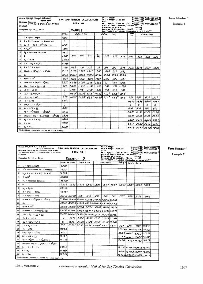
Cable 8' ~~~~~ 3~~W~~~M .~~~~3a e WeikX zw/; WAZ= W,0-9 Form Number 1(8 ccppea ~~~~ SAG AND TENSION CALCULATIONS Caliegh lsIc aAL/ft; V+AZa,3ELc.,MailmanTecnsion ttwwind W=a-j/ft -- xml5670uTension

,~.,~ FORM NO. Max. Result. Load at o*F, W-/ALWp/ft; W+A&.A&LxloExmeIP6roject D OF.Area of Croas Section, A-.0901 sq. in.Projeot ~~~~~~~~~~~~~~~Diameterof Cable, inche

Computed by W.L. Date EXAMPLE Ji~~~~~~~~odulusaof Elasticity, 1NafS xloe1coaputed by W.L. Date_____E_XAMPLE __ Coeffiolent of Linear Sxpanin cc - 72 x10'8cale ca be+/ cable onyCc5Ae,t CbeOI L. * Span Length /00092 D = Difference In Elweation 0

3 o d; d =D/ZL * d) /000 __4 8 L0/L2 .006 __

5 Ti =Maximum Tension 5670 __

8 V 1.269 .7 .87 1 .87/, .322 .3229 .322 ..322 ..871 .3272 .322 .322Tl/W 4468.1

____

8 a8 (2al - D)/L0 8.936 __

9 Z l/(d - 1/2) .1126 1.1126 .1/00 .105 .06 .08 .07 .075 .1/0/ .0676 .073/ .083810 Slack = (12/j) (l .Z2-/20) 2.1/3 2.1/3 1.667 1.840 .600 1.067 .617 .93711 so 999.4 999.4 .999.4 999.4 99~9.4 999§.4 .99,9.4 .999.4 __12 W/AEx 108 .6124 .4203 .4203 .4203 .1551 .1,551 .15.5/ .155/__113 Stretch = (W/A1)(.S2/zz) 2.720 1.865 2.099 1.998 1.293 .971 1.109 1.03 ___14 (so -La) =10 13 -.607 *.248 -~.432 -.15B -.693 .096 -.292 -.098___ __1,5 A A14 0 .855 .175 .499 -.086 .703 .3/6 .1509__ __18i L t a&S/(S~oa 0 118.90 24.39 62.5" ../'97,70 43.8" 70.8'17 t = t0*+at 00F 1/8.90 24.,3A 62..0 .y9 97.7 43.80 70.60 320 .30 0 600 /0018 aa L/2Z 4440 _ ____ *iJ 0 75396 68t0 rSeT19 tDa/L) (l - Z2/6) 0 __ ____ 0 0 0 020 X2-L/2 -19 500 Soo____0 500 500 50021 Y2 =(x2/2a) (l . X2112) ____ 216.25 16.90 /8.28 20-.9522~ Tangent Saga (LcZ/4)(1 * Z2/12) 081 __ __ __ 5.26 16.90 /8.28 20.95?2J a, =a.*D y2 4468 ___ ___ ___ 1'7.9'7M/3 52824] s.-W& 5635 ___ 4 V/l 'Z! ' 2 04 1.92/-25] T1 z Nal .5670 _4333 36' ZZ2O. /192Underlined numerals refer to Item numbers

Cable 318,000C_MA_C S.Q §jabl Weiht /.64lfft; W+AZEa.,.4204X10-CAble38,0004CAc5ASR ineSAG AND TENSION CALCULATIONS Cable Weight Plus Ice W=L.6?s#/ft; Z&~0~43 a

115/ Abize So-, Win___ S WaAaWf7r1 Form Number IMaximum Tension ftV,ia, iz talWn3.3,000 MbS. 09OF, jld,lf.8b.Vd FOMN.IMax. Result. Load at 0'?,I Wa /f; W,1AEa.tao20X1OExmpeProject Area of Cross Section, A- .39SseSq. In.Exml2Diameter of Cable, i'nche~Computed by ML. Date EXAMPLE 2 Modulus of Zlastiaity, 19a 30 xlO0O

-_________________________________

~~Coefficient of linearExpansion cca

.6 x10'

Cable+kto Wind Cable + Ice Cable Only ct(bta+- - - _____ Sa~~~~C.Cable Only9

1 L = Span Length 42792 Da= Difrerenoe in Elevation 185.5

3 Lo=L *d; da=D2/(2L d) 42834 6 La/I. .00140Z8 T1a Raximum Tension 33,000-8 W 3.322 3.322 2.623 2.623 1.684 14684 14684 2.623 1.684 1.684 1.6847 a, T1/lw 99-33.8

8 8) = (2a1 - 0)/La 4.5954

9 Z = 1/(a - Z/2) .22302 .22500 .218 .2/5 .205 .2/0 .215 .2/87 .2085 .212?8 .2/6210 Slacka (Z2/1)(1a Z2/20) 35.5266 36.-1618 33.9415 33.0116 30.005931.4907P3.011611 so 4306.9 4306.9 4306.9 4,306.9 4306.9 4306194,06.9

12 W/Alx 10 .28020_ .28002124 .22124 .14204 .14204 .1420413 Stretch a (W/AE) (S2/2Zl 11.653 7 11.5511 9.4134 9.5447 6.4268 6.2749 6.1279 __14, (So- LO) a- 10- 15 28879 24.6/07 24.528/ 23.4663 3.5791 25.2/58 26.883715 AS a 14 0 .73 78 ..6552 -.4060 ':2938 1.3429 3.010818 ~ta /S00 25.88 22.98'.-(4.24' -10-3014710'./0-5-60

Form Numbet 2 |Cable 795,OOOCi. A.CSR. SAG AND TENSION CALCULATIONS Cable Weight W= 1.024 lbs./ft.E 54aA24A1DTS-7I.C2A4AteIO Cable Weight plus Ioe W= /1 999Example 3 xum Tension FORM NO. 2 Wnd9000 Ibs 0 O'f Pt pod;al /co Et^. Wd Max. Resultant Load at OF We 2.439Projeot Aree of Cross Section Ae .7055 eq. In.Cosputed by M.L. Date EXAMPLE 3 Diameter of Cable inches

/Ce, -C /Wi 'Let - -e - -r

1 L = Span Length 12002 D = Dlfrerence in Elevation 03 L.= L - d; d = D2/(2L, d) 120048 Lc/L2 .0058 T1 = Maximun Tension 90006 W 2.439 1.999 A.999 1.999 1.999 1.99971 a = T1/W 3692

_____

8a = (21 - D)/LC 6.1569 z = 1/0a - Z/2) .1646 .1646 .1654 .1654 .1670 .1667

10 Slack = (Z2/4)(1 . z2,/2o0 5.4/5 5.415 5.475 5.475 5.575 5.56311 SO = Lc * 10 /2054 1205.4 120&4 1205.4/2054 /20S412 Tav WS0/2Z 8930 7320 7280 7280 7220 723013 Tos TaV/A /2,660.10,380 /0,320 320 10,220 10/25014 % Elongation .122 .127 .127 .135 .134 .13415 Elongation = (L4/100)So 1.470 /.530 1.530 1.628 16/8 1 6/8ic SO - Le 10 - 1 3.945 3.885 3.945 3.847 3.957 . 94517 t 0o'O 32"F 32'of"18 a = L/2Z 3640 3630 360019 (De/L)(1 2/6)20 X2= L/2-j^ 600 600 60021 = (X/2a)( + x2,12|49a4 _4 _ 49.6 50.0o |_22 Tangent tsg = (L0Z/4)(l + 22/12)23 al =a + D y2 3689 3680 3650

24 5 wa 8880 7060 7000T1 We1 9000 7360 7300

Underlined numerals refer to item numbers

Form Number 2 f Cable 795.000 C.P.A.C.S.R. SAG AND TENSION CALCULATIONS Cable Weight W= 1.024 lbs./ft.54 x.i2i4-AIum,,,u?m Cable Weight plu3 Ice We A. 9 .Example 4 Maximu T*ension 7xx.I2l4 Srteel FORM NO. 2 dResultat Load at o. 2.439

ProJect Area of Cross Section Am 7055Jq. In.Computed by M.L. Date EXAMPLE 4 Diameter of Cable Inches

rce Yz7 Ic-0 No Wind________________________ ___ nWind T-r por' 'erm=nen

1 L = Span Length /000

2 D = Differenoe in Elevation 200

3 L0-= L * d; d = D/IZL + /0/9.8 _| _|_ 6L8/Lt .006/2S T1 =Maximu Tension 9000 - ___ -

8 W 2.439 1.999 1.999 1.999 14999 1.999 1.999

al = Tl/W 3692 r L__8 a = (l2l - D)/LL 7.049 Z = 1/la - Z/2) .1435 .1435 .1455 .145/ .145/ .14 7/1 .1469

10 Slack = (Z2/4)11 = z2/2o) 3.365 3.365 3.460 3.447 3.44 7 3.539 3.52711 SO Lo * 10 1023.2 1023.2 1023.2 /023.2 1023.2 /023.2 1023.212 Tav = WSO/2z 87/0 7140 7040 7050 7050 6970 699013 Tas = Tav/A 12,320 10,120 9,970 10,000 /0,000 9,870 9,90014 % Elongation .115 .124 .123 .123 .132 .131 .131153 longation z (14/lO0)So 1/78 1.270 1.260 /260 1.352 1.340 1434018 a - Ic 10-low. 2.18 7 Z.095 2.200 2.187 2.095 2.199 |2.187 e

17 t O__0f 32'F _ 32f6 |18 a = ./Il 3485 .5446 3404 ___ __|_19 lDa/L)(l - z2/81 695 687 67670 _ __ ________20 X2 ./2.-1l9 -/95 -1057 |-/78

_____________________^2 5.44 07 __ _ 4.6r _ _ _ _ _ __ _

22 TangentSag= (LcZ/4)ll*Z2/lZJ 36.6 36.9|37.4 ___ ___ |__ |__23 al =e^* D*Y2 3690.4 36.fZ/ 13608. _ _ _ _

24I W ah8500 ___ 18.901 1_ 168001 1 _1__125 T1=~ a1l 9000 7300 |____ 72/0___ _____ __ -Underlined numrals refer to item numbers

1568 Landau-Incremental Method for Sag-Tension Calculationls AJEE TRANSACTIONS

are included: one for level spans and one The next steps are to calculate tempera- Columns 9 to 12, inclusive, are calcula-for nonlevel spans. For this purpose, pre- tures corresponding to arbitrarily as- tions of sags and tensions for particularviously published examples are used so sumed values of Z. Columns 2, 3, and 4 temperature and loading conditions. Inthat a comparison with current methods are such calculations for W= 0.871 (cable each case the value of Z for the particularof calculation may be had. In each case +ice loading) while columns 5 to 8, in- temperature is obtained from the "Z-the cable characteristics and maximum clusive, are for W= 0.322 (cable only). temperature" curve, Figure 3. Calcula-loading conditions are stated in the head- In sequential order the calculations ofing of the form. column 2 are:

EXAMPLE NUMBER 1. CALCULATED ON 6. W = 0. 871FORM NUMBER 1, WITH 1,000-FOOTLEVEL SPAN1 AN CNTA MODULUS 7. Z = 0. 1126 Arbitrarily assumed valueLEVEL SPAN' AND CONSTANT MODULUS

OF ELASTICITY Z2 ~~~~~Z2\OF ELASTICITY 10. Slack=-I 1+2-- =2.113The calculations are set forth in colum- -

nar arrangement, the first column being 11. So = 999.4 Unstressed length of cablefor the condition of miaximum tension at at 0 degree Fahrenheit0 degree Fahrenheit and maximum load- W

12. - X 106 = 0.4203 Value corresponding to W=0.817ing. AEColumns 2 to 8, inclusive, are calcula-

tions of temperatures corresponding to 13 Stretch __S 999-1.28650.4203X10-6X 99942tions =~~~~~~~~~3trth=1.85 0.40 1 6x1.865various assumed values of Z, from which AE\2Z 2X0.1126"Z-temperature" curves Figure 3 are pre- 14. (SO-Lc) = 11-13 = +0. 248 2.113-1.865 = +0.248pared. 15. AS=(14 Column 2) -Columns 9 to 12, inclusive, contain cal- (14 Column 1) =0.855 0.248-(-0.607)=0.855

culations of sags and tensions for variousselected temperatures, the values of Z 16. At= AS/(So o) = 118.9 0.855 = 118.9being obtained from the "Z-tempera- 999.4X7.2X10 =19ture" curves, Figure 3. 17. t=to+ At = 118.90 Since tO=0 degree Fahrenheit; t0+

In detail the calculations are as follows, At = 118.9 °the underlined numerals in all cases re-ferring to item numbers. For column 1,in sequential order:1. L =1,000 Span length W S02 0.6124X10-6=999.4213. Stretch= - - =2 7202. D =0 Level span AE 2Z 2X0.1126

=27203. Le = 1, 000 D = 0; therefore Lc = L

14. (SO-Lc>== 10-13 = -0.607 2.113-2.720==-0.6074. 6Lc/L2 =0. 006 6X 1, 000/1,0002= 0.006

15. AS =0 AS is the change in length5. TI = 5,670 Maximum tension due to change in tempera-

6. W = 1.269 Weight per foot at maxi- ture. This being themum loading conditions initial temperature, there

7. al=T,/W =4,468.1 5,670/1.269= 4,468. 1 is no change in length8 a -D= (2X4,468.1-0) 16. At=AS/(S c) =0 0/(SOXc)=0

8. c =8.936 =8.936 17. t =00'F Initial temperatureLc ~~~~~~~~1,000

9. Z= =0.1126 -=0.112; 18. a= =4,440 1,000/2X0.1126=4,440

2 ~= 1 =0.126Z 8936 02/2 126 19. I _ =0 D=0, therefore 19=0

Z2/ZI\ 0~~~~.112621 0.11262\ L 6

10. Slack = (1+2- =2. 113 1+ 1 2.113 20. L2=--19 =500 1,000 _0_5004 \ 20/ 0.006 20 /2 -2

12. X 100 =0.6124 - for maximum loading 221. Sag y2 1 +X

28.15 1+ 0AE AE 2a 12a2/ 2X4,440 12X4,4402/

=0.6124X 10 -6 = 28.1511 & 13. 22. Tangent sag*

WS0th=2°i= L0 Z1+2\ =2.1,OOOXO.1126i i+0.11262\

=28. 15Assume So = Lc+slack =1,000+2.1 =1,002.1

1,002.12 23. a1=a+D+y2 =4,468 (4,440+0+28)=4,468Thentreth=0612410 2X20.126=.3 24. H=Wa =5,635 4,440X1.269=5,635

11. So=Lc+slack -stretch =999.4 1,000+2.1-2.7=999.4 25. T = Wa1 =5,670 4,468X 1.269=5,670

* This being a level span, the sag y2 and the tangent sag are identical.NOTE. Item 23 should equal item 7, and item 25 should equal item 5.

1951, VOLUME 70 Landau-Incremental Methodfor Sag-Tension Calculations 1569

tions of items 18 to 25, inclusive, are then stretched) at 32 degrees Fahrenheit, T WS (14)made in Column 1. Z= 0.1654. Proceeding down column 3, 2Z

items 18 to 25, inclusive, are calculatedEXAMPLE NUMBER 2. CALCULATED ON as in column 1. Coth z= 2T1 - WD (I5)FORM NUMBER 1 WITH 4,279-FOOT Columns 4, 5, and 6 give the calcula- WSNONLEVEL SPAN3 AND CONSTANT tions for the "Permanent" condition L [D Z 1MODULUS OF ELASTICITY (cable prestretched) at 32 degrees Fahren- x =-4nasinh nizJ (16)These calculations are similar to those heit, 1/2-inch ice, no wind. From the foregoing equations by substitu-in Example Number 1. Due to the dif- EXAMPLE NUMBER 4. CALCULATED ON tion, transposition, et cetera:

ference in elevation, the straight line EXAm NUMBER 4 CALCULATED ON Letdistance between supports, L, is greater FORNUMBER 2WITH 1,200-FOOTthan the span length L; also the tangent NONLEVEL SPAN WITH VARIABLEMOD-(b dfi i) (17)sag and sag Y2 have different values. Fig-ure 4 is the "Z-temperature" curve for The calculations of Example 4 are Substituting equation 17 in equatioin 10this example. similar to those for Example Number 3. 2a,-D

a= (18EXAMPLE NUMBER 3. CALCULATED ON LcFORM NUMBER 2 WITH 1,200-FOOT Appendix. Derivation of Combining equations 10 and 15LEVEL SPAN2 AND VARIABLE MODULUS Formulas cOF ELASTICITY Coshz Q (19)This calculation makes use of the stress- Let the conductor be represented by the Z

strain curves, Figure 3. Curve A-B, Figure 5. whereAs in thesolution ofproblems,Ex- The fundamental formulas of the caten-AS in the solution of problems, Ex- ary referred to the point where it has a hori- D 2

ample Number 1 and Example Number 2, zontal tangent are: 1 Lcalculations at maximum tension and Q= (20)loading conditions are made in column 1. y=a cosh --1) (5) +1±({ Y(t

Sequentially the calculations of items a / \L/ sinh Z1 to 10, inclusive, are similar to those . x Transformingand simplifying equation 19described previously. s=a snh -a (6)The operations in items 1I to 17, in-

clusive, are

14. Per ceit elongation =(. 122 From O° Fahrenheit, curve11. So=Lc+10 = 1205.4 1,200+5.4= 1,205.4 Figure 3 for Tas= 12,660

WSo 2.439X 1,205.4 15. Elongation (14 )100)S0= 1.470 0.122/100X 1,205.4 = 1.47012. Tavg= = 8,930 -=8,9302Z 2 X 0.1646 16. So-Lc = 10-15 =3. 945 5.415-1.470 = 3.945

13. Tas=- =12,660 =--12,660 17. t =00 F Temperature at maximtumA 0.2055 tension and loading

Calculation of items 18 to 25, incluisive, The horizontal component of tension at 1are similar to those previously explained any point on the suspended conductor is: Z= + . (21)in Example Number 1. H= a (7)-Columns 2, et cetera, indicate the cal-

culations of "Temporary" and "Perma- The tensioni at any point on1 the suspended Figure 6 shows the relationiship between Qconductor is and Z for various values of DIL. It isnent"' sags and tension at 32 degrees Fahr- eietta a egnrlycnieeenheit, 1/2-inch ice, no wind. Under Tl= Wy±H= W(y+a) (8) to be unity without loss of accura y.wthese conditions W=1.999. The following equatioils are derived in Expanding (z/sinh z) as a seriesA method of successive approxima- "Tranismission Line Catenary Calcula- z / Z2\

tions is used. Referring to column 2, a tions.'4 sn Z 1- |+ (22)value of Z=0.1646 is assumed; calculat- Lsinh Z 6ing items 9 to 16, inclusive, in a similar Z - (by definition) (9) Substituting equation 22 in equation 16manner to that indicated in column 1, we 2-L -D/Za\1

2T____WD L- asn11I-+..I (3have item 16,(S0-L,) = 10-15=3.885. V2 W (10) X= 4a sinh- LL\1-/+J (23)The value of 16 should be 3.945 2 LetThe difference of these to values is 0.060 Slack=S-Lc= ~Z2I 1+- J± ... (11)Adding slack, column 2 5.415 6Lc \ 20/ sinh-'[P(1-4

545 Tangent sag=-L-.+3L Dz+p z >/(4for slack= 5.475, we calculate the value of LZ 2Z=0.1654 completing calculation of items -4 ...2 (12) Sbtttneuto2ieuto2

12 to 16, inclusive; in column 3 we getitem16, SO-Lc=3.945, therefore, for the Sr tch= S 13 FaD/Z2\1)] 25temporary condition (cable not pre- AE 2 LL\6/

1570 Landau-Incremental Alethodfor Sag-Tension Calculations AJEE TRANSACTIONS

Values of P are plotted on Figure 7. It D2 H= Wa (J)can be seen that for ordinary values of D/L, dLaL+d;where d=2 (A)P may be considered to be unity. Expand- LdL DP _ / (K)ing equation 6 as a series a==2 LL \ 6/

x2 x2 ai-j B x22r X22 \y 1+_+... ~~~(26) Y2 L1 ± -l-l(L)2a 12a2 2a, -CD 2a L 2a /6a)JNeglecting terms beyond the 2nd as negli- Lcgible

Z 1 z (D) ReferencesX-F V+z 1 2-7 - 1. SAG CALCULATIONS BY THE USE OF MARTIN'Sy=_2a L + 2aA\6a (27 2 TABLB (book), James S. Martin. Copperweld SteelZ2/ Z2 Company, Glassport, Pa., 1931.

The equation of the straight line distance Slack 01J (E) 2. ACSR GRAPHIC METHOD FOR SAG CALCULA-between supports is (6- 2

TIONS (book). Aluminum Company of America,\ L2 / Pittsburgh, Pa., 1927.

Lc= VL2+D2 (28) 3. MIssissIPPI RIVER CROSSING OF CRYSTAL CITYTavgS TRANSMISSION LINE, H. W. Eales, E. Ettlinger.Let Stretch =- (F) AIEE Transactions, volume 44, 1925, pages 387-Let Stretch=~~~~~~~~~~AE 97.

Lc =L+d (29) Ws 4. TRANSMISSION LINE CATENARY CALCULATIONS,Tvg=- (G) D. 0. Ehrenburg. Electrical Engineering (AIEE

then 2Z Transactions), volume 54, July 1935, pages 719-275. TRANSMISSION LINE CATENARY CALCULATIONS,

D2 LcZ z2\ (letter), H. J. McCracken. AIEE Transactions,d (30) Tangent sag= il+-I (H) volume 54, August 1935, page 910.

6. BROKEN CONDUCTOR EFFECT ON SAGS IN

Sumiimarizing the foregoing equations and L SUSPENSION SPANS, Alflo Bissiri, Maurice Landau.S.mmariingtheforegoig equatonsan a = (I) AIEE Transactions, volume 66, 1947, pages 1181-rearranging their order 2Z 88.

No Discussion

1951, VOLUME 70 Landazu-Incremental Method for Sag-Tension Calculations 1571