INCREMENTAL VOLUME RENDEREING ALGORITHM

FOR INTERACTIVE 3D ULTRASOUND IMAGING

R Ohbuchi and H Fuchs

Department of Computer Science, University of North Carolina at Chapel Hill,

Chapel Hill, NC 27599, U.S.A.

Abstract

This paper describes a medical 3D ulwasound imaging system that incrementally acquires and visualizes a 3D volume from a series of 2D images. The system acquires the image from a conventional B-mode 2D echography scanner, whose scanhead is attached to a mechanical tracking arm with three degrees of freedom. It reconstructs a stream of 2D images with their locations and orientations into a 3D array of regularly spaced samples, to be rendered by a modified front-to-back image- order volume rendering algorithm. Visualization is done so that each incoming 2D image slice promptly affects the rendering result. This paper concentrates on the incremental volume rendering algorithm that takes advantage of the incremental scanning to reduce image generation time per each input image slice. We describe a new fast ray-clipping scheme called D-buffer algorithm that is based on the Z-buffer algorithm. It is followed by another speedup scheme called hierarchical ray caching, and a method to efficiently integrate geometric objects with volume data in image space.

Keywords

3D ultrasound echography; Ray-casting; 3D imaging; Z-buffer algorithm; D-buffer algorithm; hierarchical ray-caching.

1. I N T R O D U C T I O N

We have been working toward a medical 3D ultrasound scanner system that will acquire and display a 3D volume in real-time. We call this system an 'ultimate' 3D echography (3DE) system. It will acquire, display, and manipulate a 3D volume image in real-time. Such 'real-fime-ness' can be crucial for an application such as cardiac diagnosis, where a static 3D image or even a dynamic display of a series of images acquired over many cardiac cycles by gated acquisition might miss certain kinetic features. The 'ultimate' system has two major components: the image acquisition part and the image visualization part. We at UNC-Chapel Hill have been working on the real-time 3D visualization part of the system, while Dr. Olaf yon Ramm's group at Duke University has been working on the real-time 3D image acquisition part of the system.

To study the issues involved in 'ul t imate ' 3D ultrasound visualization before the real-time acquisition subsystem becomes available, we have been developing an incremental, interactive 3DE scanner system. This system will acquire and display the 3D image incrementally at an interactive rate. It will use a state-of-the-art medical real-time 2D ultrasound echography scanner as an image input, where a user guided scanhead is tracked with 3 degrees of freedom. Using the geometric information acquired for each 2D image slice, the system incrementally reconstructs the 3D array of sample points spaced regularly on the Cartesian coordinate from a stream of 2D slices. These slices are located and oriented arbitrarily with 3 degrees of freedom. The system renders the reconstructed volume, again incrementally, to produce volume rendered 2D images. This visualization is done incrementally so that every new 2D slice acquired affects the final image promptly, thus offering a high degree of interactivity to the user.

We present here the brief introduction to the incremental, interactive 3DE system and the incremental volume rendering algorithm designed for a high degree of interactivity. We briefly describe the 'ultimate' system, then present a review of previous works on 3D ultrasound imaging. This is followed by the sketch

487

of the incremental acquisition and visualization system we have been working on. We describe the basic incremental volume reconstruction and rendering algorithm in section 2. Section 3 and 4 introduces enhancements to the basic algorithm. In section 3, a fast ray-clipping algorithna called D-buffer algorithm is presented, which is followed by a proposed enhancement to the idea of ray-caching called hierarchical ray- caching for faster compositing. Then, in section 4, another algorithm is proposed which combines D-buffer with the hierarchical ray-caching to allow fast integrated rendering of polygons, polyhedron defined volumes for cutaways, etc., to provide fast interaction with the volume image.

1.I. The 'Ultimate' 3D Ultrasound Scanner

Among various medical imaging modalities, ultrasound echography is the closest to achieving 3D real-time acquisition, even though other modalities such as MRI are becoming faster. The new scanner being developed by Dr. Olaf von Ramm's group at Duke University (Shattuck, 1984) will enable the 'ultimate' 3DE system to acquire 3D images at real-time rate. Due to the velocity of sound limitation (about 1540 m/s in water), scanning a 3D volume with reasonable resolution (128 x 128 x 128 or more) in real-time (e.g., 30 3D-frames/s) requires parallel processing. The new scanner will use a single- transmit/multiple-receive scheme called Explososcan to increase data acquisition bandwidth. The first implementation will use a 16 x 16 2D-array transducer along with 16 x 16 x 64 digital delay-lines implemented in VLSI chips for 3D beam steering and focusing with 64-way multiple simultaneous reception.

Once the real-time 3DE data has been obtained, it has to be visualized. We at UNC-Chapel Hill have been working on this problem. One major effort is a display system based on a volume rendering technique for visualization that will display 3DE data in real-time. Such a display system has to cope with the challenge of very high data bandwidth. The real-time 3DE scanner above will produce about 2-4 Million points per frame, or 60-120 Million points per second. Visualizing a 3D volume data of this bandwidth in real-time requires very large computational power (on the order of Giga floating point operations per second) if a straightforward algorithm is used. We are approaching this issue through parallelism and algorithm efficiency.

Providing a visualization method that is effective to the user is another major issue. It involves standard problems associated with visualization of 3D data, such as obseuration. To took at the inside of the left ventricle, various objects in front, e.g., images of fat tissue and part of myocardium, must be removed to reveal the object behind. This usually requires extensive manipulation of the 3D image data. On top of those are the additional characteristics of ultrasound data that can hinder the visualization, e.g., speckle noise, gain variation, shadowing, specular artifact. Wei-jyh Lin at UNC-Chapel Hill has been working on an algorithm to estimate surfaces in 2D echography image under the presence of speckle noise using multi-scale filtering technique (Lin, 1991). In the future, this surface estimator will be added as a front-end to the display system described above.

1.2. Previous Work in 3D Ultrasound Imaging

Many works on 3D ultrasound imaging have been done in the past. Most of the studies known to the authors have tried to reconstruct 3D data out of imaging primitive data of lesser dimension (usually 2D image), instead of directly capturing 3D data. This is due to the obvious lack of real-time 3DE scanner.

To reconstruct 3D image from images of lesser dimension, the location and orientation of imaging primitives must be available. Coordinate values are either explicitly tracked, as in (Brinkley, 1978) (Ghosh, 1982) (Hottier, 1989) (Raichelen, 1986) (McCann, 1988) (Nikravesh, 1984) (Stickels, 1984) (Mills, 1990) using mechanical, acoustic, or optical tracking mechanisms; or it is controlled implicitly at the time of acquisition (Lalouche, 1989) (Nakamura, 1984) (Billion, 1990). The most interesting recent work in the latter category is on a near-real-time, automatic 3D scanner system (Billion, 1990). This system is the closest yet to the real-time 3D ultrasound scanner, and is being developed at Phillips Paris Research Laboratory. It is a follow up to the earlier work (Hottier, 1989) which, like our system, was a manually guided scanner with mechanical tracker. This near-real-time 3D scanhead is a 'double wobbler' mechanical sector scanner, where a conventional wobbler 2D sector scanhead with annular array transducer is rotated, or wobbled, in an additional axis by a stepping motor to provide 3D scanning. In a period of 3 to 5 seconds, 50 to I00 slices of 2D sector scan image can be acquired. The use of an annular array transducer in this system will give better spatial resolution than the real-time 3D phased array system mentioned above by yon Ramm et al, but the latter will provide better temporal resolution.

For presenting the scanned result, there are two forms: non-visual, and visual. The latter can be classified further by the rendering primitives, which are either (geometric) graphic or image. The majority of the earlier studies (Brinkley, 1978) (Ghosh, 1982) (Raichelen, 1986) (Nikravesh, 1984) (Stickels, 1984) had non-invasive estimation of the volume of the heart chamber as their primary objective. Thus, often the reconstruction is only geometric. A typical process involved using a digitizer to manually trace

488

Disks

images mes/s )Opixels)

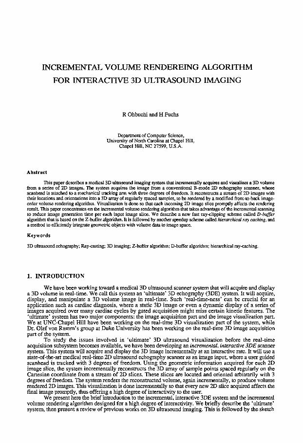
Figure 1. Incremental 3D volume data acquisition system using conventional 21) echography scanner

2DE images stored on video tape. Since the visual presentation is a secondary matter, wire frames or a stack of contours are used to render the geometrical reconstruction result

More recent studies (Nakamura, 1984) (Lalouche, 1989) (McCann, 1988) (Hottier, 1989) (Billion, 1990) actually reconstructed 3D grey level images, preserving the grey scale, which can be crucial to tissue characterization. (Lalouche, 1989) is a mammogram study using a special 2DE scanner which can acquire and store 45 consecutive parallel slices with 1 mm intervals. It is reconstructed by cubic-spline interpolation, and volume rendered. (McCann, 1988) performed the gated acquisition of a heart's image over a cardiac cycle. They volume rendered 2DE images stored on video tape. Upon reconstruction, 'repetitive low-pass filtering' fills the spaces between radial slices, which suppresses the aliasing artifact.

(Billion, 1990) uses two visualization techniques: re-slicing by an arbitrary plane, and volume rendering. The former allows faster but 2D viewing on a current workstation. The latter allows 3D viewing, but often involves cumbersome manual segmentation. The reconstruction algorithm is a straightforward low-pass filtering.

1.3. Incremental, Interactive 3D Acquisition and Visualization

To study the issues of real-time ultrasound 3D echography visualization before the real-time 3DE acquisition system becomes available, we have been studying an incremental, interactive 3D echography (3DE) system. In this system, a user-guided scanhead mounted on a 3 degrees of freedom (3 DOF) mechanical tracking apparatus will acquire a series of 2D image slices as well as the corresponding geometries, i.e., location and orientation, of each slice. Using these geometries, regular 3D volume data, where sample points are at uniform intervals in Cartesian coordinates, axe reconstructed from a series of 2D images with irregular geometries. This reconstruction process and the following volume rendering process take place incrementally as each new 2D image slice arrives. Each new 2D image will affect the final rendered image without waiting for the rest of the slices to arrive. (Since scanning may continue for an indefinite period of time, possibly sweeping the same volume many times, waiting for the 'rest' loses its meaning.)

Figure 1 shows the image acquisition system for the incremental, interactive ultrasound scanner system (See Figure 2a for the picture). The 2DE scanner mounted on a mechanical tracking arm with 3 DOF acquires 2D image frames at a maximum rate of around 30 frames/see. Each 2DE image slice from the ultrasound scanner is video-digitized in real-time by a Matrox MVP-S video digitizer board and copied into a SUN-4 workstation. Due to the MVP-S's frame buffer design, this copying process is relatively slow, running at 5 frames/s for 256 x 400 pixel images.

The potentiometers in the 3D tracking arm transduce the coordinates and orientation (x, y location and angle 0) of each of the image IYames through a Data Translation DT-1401 A/D converter board. The

489

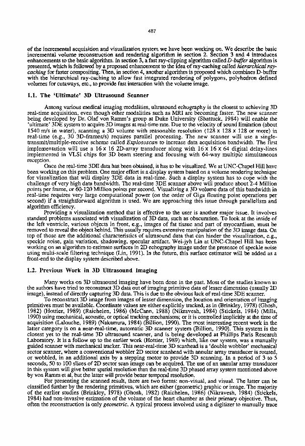
Figure 2a. (Left) Scanning setup for the incremental, interactive 3D ultrasound scanner system. Figure 2b. (Right) The doll phantom. The height is about 17 cm.

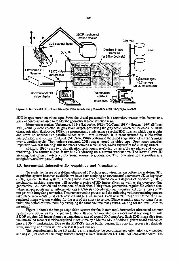
Figure 3a. (Left) A 2D echography image of the torso section of the doll phantom. Figure 3b. (Right) Reconstructed and volume rcndered image of the phantom.

tracking system has an accuracy of about 1 mm in x-y position and a maximum sampling rate of around 800 sample/s. The arm came from the previous generation 2D echography scanner Rohe ROHNAR 5580. ROHNAR 5580 used tracking to generate 2D images from a 1D scanhead. In our system, tracking is used to generate 3D volume from a state-of-the-art 2D scanner.

The system acquires image and geometry only if the change in geometry exceeds a certain preset threshold. This regulates to some degree the spatial sampling rate. Since the scanning of the 3D volume takes some time, the object must be stable enough. Examples of possible imaging targets are a liver or an immobilized woman's breast. We do not consider the scanning of a moving target, such as a beating heart, as an objective.

This acquisition setup is similar to the work at the Paris Phillips Research Laboratory by Francois Hottier et al (Hottier, 1989), which used a similar mechanical tracking arm. In their work, scanned 2D images and the scanhead tracking result are stored on a video tape and a PC ' s disk, respectively. Images and their matching geometry values are selected later off-line. We have used the real-time video digitizer and the tracking arm to acquire image and geometry at the same time.

490

Acquired 2DE image slices are incrementally reconstructed by local interpolation into regularly sampled 3D volume data by merging the new data with the existing volume data. As the slices accumulate into 3D volume, the rendering takes place, which shows the buildup of 3D volume. We will describe the details of the incremental volume rendering algorithm later in this paper. One thing of note is that the volume can be scanned repeatedly, to get better spatial sampling or to gain a a better acoustic window (e.g., to avoid bones). The reconstruction algorithm considers these modes of use, and provides reconstruction buffer update policies that include 'complete replace' and 'replace by weighted average'.

CtLrrently, we store the images and coordinates into a disk of a file server connected by Ethernet for later reconstruction and rendering experiments on workstations such as DECStation 3100. In 1991, we hope to demonstrate a system that will use a powerful graphics multicomputer, Pixel-Planes 5 (Fuchs, 1989), for parallel reconstruction and rendering. In this parallel system, we expect the incremental visualization process to take place at an interactive rate of more than a frame per second without ever storing the image onto the disk. As mentioned, image read-out from the video digitizer is slow, and this might limit the processing speed of the entire system to about 5 frames/s acquisition rate. Assuming a 4 mm elevation resolution of the scanner image slice and a Nyquist sampling rate of 2 ram, a target volume of 20 cm thickness can be scanned as 100 slices of equally spaced parallel planes. Scanning the volume with 50- 100 slices will take 1.4-3 s, assuming a 30 2D-frames/s acquisition rate, or 10-20 s, assuming a 5 2D- frames/s acquisition rate.

We have conducted a preliminary data acquisition and rendering experiment, which is reported in (Ohbuchi, 1990). We used an ATL Mark-4 scanner with a 3.5 MHz linear scanhead as the image input, and scanned a phantom (baby doll, in Figure 2b) and a human forearm in a water bath. Figure 3a shows the 2D echography image of the doll phantom. Figure 3b shows the reconstructed and rendered image of the doll from 90 slices of roughly parallel, roughly 2 mm interval 2D image slices. It is incrementally reconstructed using a forward-mapping octahedral kernel reconstruction algorithm, which will be explained later.

2. INCREMENTAL VOLUME VISUALIZATION

In this section, the algorithm for the incremental, interactive visualization of 3DE images from a sequence of 2DE slices is presented. We can divide the visualization stages of the incremental, interactive 3DE system into two major stages; reconstruction and rendering. The emphasis in this paper is on the incremental volume rendering algorithm.

Figure 4 shows the pipeline of the incremental volume visualization. Video digitized 2DE image slices from the scanner are incrementally reconstructed into a 3D scalar field sampled at uniformly spaced 3D grid points on a Cartesian coordinate system. Reconstruction is done into a reconstruction buffer, which resides in the world coordinates. It is then rendered using a modified front-to-back image-order volume rendering algorithm as developed by Levoy (Levoy, 1989). A reconstructed 3D scalar field in the reconstruction buffer is classified (non-binary classification) and shaded to produce a 3D shade buffer that also sits in the world coordinates. The next steps are the ray-casting process, where sample points in the world coordinates are transformed into 3D screen coordinates and then composed into 2D screen coordinates to yield a volume rendered image.

2.1. Incremental Volume Reconstruction

Several different approaches are possible to visualize irregularly sampled volume data. Theoretically, a stream of 2D image slices with variable geometry can be rendered directly by a certain rendering algorithm. Some algorithms to directly render irregular data samples have appeared recently (Garrity, 1990) (Wilhelms, 1990) (Miyazawa, 1991) (Neeman, 1990) (Shirley, 1990).

We have chosen to reconstruct regularly sampled 3D volume data in the reconstruction buffer, which is then rendered using more or less conventional volume rendering algorithms that expect volume data samples at regular 3D grid points. One reason for this is the speed of rendering. Once reconstructed, the volume data sampled on a regular 3D grid stored in 3D array with implicit geometry and connectivity offers easy access to the data. Another reason is that we wanted to allow multiple scanning sweeps of the target volume by the scanhead. 2D images from multiple passes are merged into a single image. Achieving this with direct rendering requires storing a large, unknown number of raw input image slices, and this is neither memory nor computationally efficient.

In designing the visualization scheme, we assumed that the target scalar field being sampled is continuous. Thus, if the target volume is sampled with a sufficient sampling rate by the 2D image slices, the resulting image of the target volume generated from these 2D slices must be continuous. For example, the resulting image should not look like a set of intersecting image planes with empty spaces in between. This means that the reconstruction requires some form of interpolated resampling. We have to be careful

491

Irregular 3D object Regular 3D object 3D screen 2D screen coordinate coordinate coordinate coordinate

I I I I I I I I

mage ~ - ~ [ dat~l r r t data i - Y l data- J ' l r l data lice X ~ ~"'~J . . . . i ~ I ~ a n s f o ~ a t l o n / ~:~oosit ing

. . . . . . . . . . . . ~ ~ .mn~ing - ~

Transform and merge a new image plane atarbilrary ,angle & 10~tion

Reconstructed 3D image data

Insert a new r e ~

J/ll ! 2D SC / I S

Ray c o m p o s ~ ~

Figure 4. Incremental volume visualization processing stages. Irregular data slices are first reconstructed into regularly sampled 3D volume data. The volume data go through a standard volume rendering process, but the processing is confined to the inside of the slab formed by the last two image slices.

about interpolation. If the sampling rate is not sufficient, there is no way to recover information that was not sampled upon acquisition. The user should be made aware, by some means, of the undersampling..

We try to reconstruct a 3D array of sample points at regular intervals on Cartesian coordinates from a series of 2D image slices with 3 DOF as the imaging primitive. We assume that there is a rectangular volume in the real-world we are imaging, which will be sampled by points uniformly spaced on the 3D Cartesian coordinates. The system discards the sample points on 2D image slices that are outside this rectangular volume.

The next question regards what interpolation techniques to use. One important characteristic of our visualization scheme is that each input image must promptly be reflected in the final image. Thus, the interpolation method used for reconstruction can not be what Franke (Franke, 1982) calls the 'global ' method of interpolation, where the interpolant is dependent on all data points. Both of the two reconstruction methods we have implemented so far are the ' local ' kind.

Ideally, the interpolation function should depend on the imaging system. We have discovered, from the images obtained by scanning a 3D geometric calibration phantom made of thin wires and beads, that the image slice is fairly thick. A 2 mm bead is visible on the screen after 4 to 5 nun translation of the scanhead in elevation direction. This suggests much lower elevation resolution than the range resolution. Also, as expected, the sampling function in the far view is fuzzier and larger than in the near view. Though this was not quantitative, this gave us a feel of the shape of the sampling functions to expect.

We are still experimenting with the reconstruction algorithm. One method we have tried is a forward mapping algorithm, where the input sample points in the 2D image slices are distributed to the reconstruction buffer grids around the input sample points using a small spatial filter kernel (Figure 5). The kernel is anisotropic, and its size is determined in the input parameter file to the program. Mostly, we have used a filter kernel with octahedral shape in 3D that has the long-axis of around 6 mm and two short-axes of around 3 mm. This shape resembles the estimated shape of the ultrasound scanner system's sampling function. This corresponds to 12.5 x 6.2 x 6.2 voxels in the reconstruction buffer. Since the sampling function is attached to the image slice's coordinate, the kernel rotates with the input slice. For each orientation of the slice, coefficients of the octahedral kernel are computed on-the-fly on the discretized x-y-z grids of the voxels. The 2D weight buffer in the diagram accumulates the weight of the kernel for later normalization. The age buffer records the staleness of the image in the reconstruction buffer to help determine the weight with which to mix the old value in the buffer with the new contribution.

Another reconstruction algorithm is a backward mapping kind, where the algorithm traverses the reconstruction buffer grid, while the nearby sample values from the last two input image slices are linearly interpolated and collected. This is only C o continuous, and its C ~ discontinuity tends to show up in the image by a gradient approximation operator in the shading stage. Though it is fast, this algorithm does not produce as good a result as the one above.

We will continue to do more research in this area to find satisfactory reconstruction with small enough computational cost for interactive visualization.

492

f

Forward mapping by a filter kernel

..... ~;~;~,. Filter kernel ,~ii~ ~.~

Grid 0oints affected

~x

f

Backward mapping by linear interpolation

l ~ . Input image pixels

~ ~'~._, ~ .......... 0 Innt~earl~iCa~ed points 0 Inter-slice

interpolated points Buffer (3D)

Figure 5. Reconstruction buffer and two reconstruction algorithms implemented; forward mapping using small filler kernel (above) and backward mapping algorithms.

2.2. Incremental Volume Rendering

Once the volume data with regular 3D sample points is reconstructed, it can be rendered using a standard volume rendering algorithm as described in the literature (Upson, 1988) (Sabella, 1988) (Levoy, 1988). As is known, volume rendering can be computationally expensive. We have to make the cost of image generation from reconstructed data low enough to achieve the goal of interactive image generation rate on moderate scale hardware.

The incremental volume rendering algorithm tries to reduce computation by taking advantage of three characteristics of the scanning process: 1) 2DE image slices are acquired incrementally, 2) shading parameters will not change for every few frames, 3) viewpoint will not change every few frames. If we assume these conditions to be true, we can perform incremental rendering. By incrementally shading and ray-sampling per each acquired image slice, the system limits the computation to the 'slab' formed by the last two inserted images, instead of the entire volume of the reconstruction buffer. With fixed viewpoint, incremental ray-sampling is realized by caching the tri-liniear interpolated ray samples from the previous slabs in a 3D array in the 3D screen space called ray cache. Ray-cache separates relatively expensive ray- sampling operations from relatively inexpensive ray-compositing operations. Ray-compositing is performed for an entire ray span inside the reconstruction buffer for each frame.

Figure 4 shows the process of incremental volume rendering. After the reconstruction, classification is done by table look up, and then the shading values of color and opacity are computed. The classification and shading take place only inside the slab formed by the current and previous image slices. Currently, we have implemented two shading algorithms: 1) image value shading that directly maps from input scalar value to the color value by table look up, and 2) object-space-gradient Phong shading. The latter performs Phong shading with ~ u s e and specular components where normal vectors of the field are approximated by finite difference computed in the object space. We included the method 1) for its efficiency, though the method 2) can emulate 1). Shading method 1 ) combined with additive compositing produce synthetic radiograph image quickly, which is useful to find better viewpoints. The shading results is stored in a shade buffer (3D) that resides in the world coordinate.

The ray-sampling stage performs ray-casting, where a ray is cast from each pixel into the shade buffer, and the shading values are sampled at uniform intervals along the ray. We provide perspective projection which is hoped to give better 3D perception. Perspective projection can cause over and/or under sampling problems in ray-casting. Scheme to correct aliasing due to perspective projection, such as (Novins, 1990), is not employed in our current implementation. A ray sample is the result of tri-linear interpolation of values from eight vertice of cube enclosing the sample point. This stage also works incrementally, and only the same sub-volume processed in the shading stage is sampled. The system clips the ray to the slab (Figure 6a and 6c), to sample only inside the slab. We developed an algorithm that is

493

Reconstruction ~ A Buffer . ::~creen ~ _ . /

Last slab a d d e d ~ R a y ~ _ , ~ i e e ~ >

- - I I / A veSeQm,

| , d l [ r ActiveSegment [ j r ] Exit _ _ ~ Active segment

/ ,~ r BoxExit [ / ~ Active segment to be sampled

a) Clipping rays to the slab and reconstruction buffer for sampling and compositing.

b) Concave slab with up to 4 intersections

c) Convex slab with up to 2 intersections

Figure 6a. (Left) A ray from a pixel is clipped to the reconstruction buffer bounding box, and to the last slab for compositing and sampling, respectively. Figure 6b. (Right Top) Slab can be concave, with up to 4 intersections, or Figure 6e. (Right Bottom) convex with up to 2 intersections.

essentially the same as the Cyrus-Beck clipping algorithm (Cyrus, 1978) for this clipping. The slab is decomposed into two convex polyhedrons if it is concave (Figure 6b).

A 3D array called ray-cache in 3D screen space saves the ray sample values. This is a classic space- time trade off. Each pixel in the frame buffer is associated with a linear array of ray samples along the ray. As the new slab is shaded and sampled, those samples are inserted to the appropriate locations (depth) in the ray-cache, replacing the old value. The shade buffer voxels outside the slab are not sampled and the ray sample values for these remain unchanged. Current choice of compositing include multiplicative compositing as in (Levoy, 1988), additive compositing for X-ray like image, and Maximum Intensity Projection that takes the maximum sample value along the ray as a pixel value.

If multiplicative corrrpositing is used, we must composit an entire span of the ray that lay inside the reconstruction buffer, even if only a portion of it are new samples. (We ignore the adaptive ray termination here for simplicity, though it is implemented.) But since relatively expensive interpolated ray-sampling (and shading) is limited to the inside of the slab, separating ray-sampling from ray-compositing saves time. The span of the ray to be composited is obtained by clipping the ray to the reconstruction buffer bounding box.

Note that the above arguments about incremental volume rendering assumed fixed viewpoint as well as fixed shading parameters. If viewpoint changes, ray-sampling and compositing need be done essentially on the entire volume. If the classification and/or shading parameters changes, classification and shading in addition to ray-sampling and ray-compositing must be done. In volume rendering, change of density classification function to classify desired object (e.g., to render either skin or bone as a surface from X-ray CT images) is as frequent as change of viewpoint. Thus, both of these two operations must be fast. Various forms of coherence, such as image and object coherence as well as temporal coherence can be used to improve performance. But current implementation does not include optimizations for the non-incremental cases.

3. IMPROVING RENDERING PERFORMANCE

Our goal is to make this system as interactive as possible. It should run with the image generation speed (reconstruction and rendering combined) of more than 1 frames/s, at the slowest, on the proof-of- concept system using Pixel-Planes 5.

In the interactive, incremental 3DE system the volume data change every image frame. Many of the conventional optimization schemes that assumed multiple image generation from single data set can not be applied to such a case. For example, skipping empty space by hierarchical space enumeration, using octree, will not be appropriate since octree is usually precomputed. Similar argument goes to the precomputing the gradient vectors or complete shading (color and opacity) values.

Also, use of incremental scheme tipped the scale in relative costs of various stages of volume rendering. A good example is clipping the rays to the volume of interest (i.e., to the reconstruction buffer

494

bounding box). It was a minute part of ray-casting process in the conventional ray-casting based volume rendering. In the incremental algorithm, relative cost of ray-clipping has become a significant part of ray- casting process. This is because a volume to be sampled (i.e., a slab) is much smaller and the clipping need be performed for every input slice. This overhead is expected to worsen if the algorithm is parallelized by subdividing the reconstruction buffer in object space. Shading (Phong shading) and ray-sampling still remains as the other major parts of the rendering process, as well as the reconstruction depending on the reconstruction algorithm used.

3.1. Ray Clipping by Scan Conversion

With the introduction of ray-cache, ray-sampling the unchanged part of the volume outside the slab is obviously wasteful. To sample rays only in the slab formed by latest two slices, each ray from the pixel is clipped to the slab. As mentioned, we used an algorithm similar to Cyrus-Beck (Cyrus, 1978) in the first implementation. As seen in the Table 1, clipping rays to the slab has taken up large portion of rendering time. We needed a faster algorithm.

We have developed a new line-polyhedron intersection algorithm called D-buffer algorithm for Distance Buffer. It is not as general as the Cyrus-Beck clipper, but much more efficient if applied to computing intersections of non-trivial number of rays from a screen with polygons. It takes advantage of the efficient polygon scan conversion algorithm to compute intersection distances (see Figure 7a). Following is the sketch of the D-buffer algorithm for ray-clipping.

{ This routine computes the intersection of all the rays from the screen pixels with the slab defined by polygons, using polygon scan-conversion. } procedure RayClip(Slab) begin

• If the slab is concave, decompose it into the convex polyhedrons. for each polyhedrons

• Clip it to the reconstruction buffer bounding box. Clipped faces must be 'closed' by adding new polygons.

for each polygon that forms the polyhedron, • Transform it into the viewing coordinate, and clip it to the view volume. • Scan convert the polygon into D-buffer, using PixelUpdate0 for each pixel.

end;

{ Polygon scan conversion routine calls PixelUpdate0 per scan converted pixel (u, v, n), to update the D-buffer. (u,v) is the location of the pixel on the screen while n is the screen Z value (real) of the scan converted point. } procedure PixelUpdate(u, v, n) begin

• Compute the Euclidean distance from projected 2D point (u,v) in 3D screen space, to its back- projected point in 3D screen coordinate (which is the intersection).

• Insert the distance for pixel (u, v) to the corresponding entry of the distance list, which is sorted by the distance.

end .

In the PixelUpdate0 routine, if the projection is orthogonal, scan converted screen Z value is the Euclidean distance from the pixel to the 3D point projected to that pixel. If the projection is perspective, the distance must be computed by back-projecting the pixel into 3D screen coordinates.

Computed distances from the pixel to the intersections with the polygons are kept in the distance list for each pixel (See Figure 7b). This list is kept in ascending order as intersection distances are inserted. A ray has either two or four intersections with a slab, so our implementation has a 4 position array for the distances. After two or four intersection distances are obtained, we have to determine the interval(s) where the ray is to be sampled. They are the distances in 3D screen space from the screen pixel to the entry and exit intersections of the slab. All the polyhedrons are convex here so that the paring of the intersections to the intervals can be made by the parity rule. This is assured (in non-singular cases) by making the polyhedron closed. To be more general, the 'sidedness' of the polygon (i.e., which side is facing the viewpoint) can be used to pairup the interval. The sidedness is determined by the sign of innerproduct of the polygon's surface normal and the view vector, which is done once per polygon. This is not necessary to clip rays to the slab, but it is useful later when integrating the volume image with the polygonally defined objects using D-buffer.

495

Distance from pixel to intersection ~ ~ 1 1 ~ % ~ Sereenpixel,~r\

3doSCreen ~ . ' ~

J

Scan-converted polygon

a) Ray-intersection by polygon scan-conversion

v

Ray-cache /

i,, I I I I I I .... I I

n be bx

screen

b) D-buffer with linear ray cache (LRC)

Figure 7a. Ray-polygon intersection can be computed efficiently by scan conversion. Figure 7b. D-buffer has 1D arrays for ray-cache, as well as distance lists for up to four intersections.

D-buffer structure has a few other fields per pixel, as seen in Figure 7b. One is the ray-cache, a 1D array to store sampled ray values. The interval to be composited is stored in be and bx pair, which are the entry and exit to the reconstruction buffer bounding box. If a ray from a pixel needs compositing, it is marked in field t. Numbers of intersections are stored in n as slab polygons are scan converted.

This D-buffer algorithm exploits the geometric coherence in the polygons that forms the slab being intersected, through the polygon scan conversion algorithm (Foley, 1990). Using polygon scan conversion algorithm limits the computation to only those rays that actually intersect the slab. This is in contrast to the clipping algorithm based on conventional ray-polygon intersection where all the rays must be checked for intersection before they are rejected. Also, due to its incremental nature, for a non-trivial number of intersections, cost per ray is very small.

We have implemented the ray-clipping by D-buffer, as well as the Cyrus-Beck algorithm. Table 1. compares the execution time of various visualization stages per single image generation for three different algorithms: without ray-clipping, ray-clipping by Cyrus-Beck algorithm, and ray-clipping by D-buffer algorithm. In all three cases, reconstruction (backward-mapping algorithm) and shading (Phong shading) are incremental. The backward-mapping reconstruction algorithm used is fast but not of high quality. It is very likely that the computational complexity of the reconstruction will increase in the future as reconstruction quality is improved. The program written in C language is compiled with -O option and executed on the DEC 5810 with 256 MByte of memory which is running Ultrix operating system. As an input, 36 2D image slices of roughly 5 mm intervals are read from a disk file along with their geometries. 34 images of 256 x 256 pixels each (whose 34th image is similar to Figure 3b) are generated. Time for the disk access is excluded from the timing. We measured timings by UNIX system call l:±rnes ( ) for the program to generate 34 images, which is then divided by 34 to obtain average timings per frame.

Table 1 shows great reduction in ray-sampling time by incremental ray-sampling, i.e. by limiting the ray-sampling to inside of the slab by ray-clipping. Table 1 also shows that the D-buffer algorithm virtually removed ray-clipping overhead. Time in the sampling stage is now spent almost entirely in the tri-linear interpolated resampling. Further speed up of ray-sampling will require such optimizations as skipping empty spaces, or adaptively reducing the number of rays cast.

As mentioned above, the relative cost of the reconstruction may increase as the reconstruction

Table 1. Execution time of ray sampling and compositing for the three cases: no-clipping, clipping with Cyrus-Beck clipper, and clipping with D-buffer algorithm. Both reconstruction and shading stages are done incrementally on all three cases. Numbers in parenthesis are the relative time spent in percentile.

Processing Stages ..... No Clipping Cyrus-Beck Clipping ...... D-buffer Clipping i , H I I I , I M

Reconstruction 0.60s (0.3%) 0.60s (3.3%) 0.59s (5.9%) Shading 2.87s (1.4%) 2.83s (15.4%) 2.81s (28.3%) Ray-clipping 0.00s (0.0%) 8.40s (45.8%) 0.10s (1.0%) Ray-sampling 185156s (91.8%) 4175s (25.9%) 4.67s (47A%) Ray-compositing 13.13s (6.5%) 1.77s (9.6%) 1.75s (17.6%) Total time 202.18s 18.35s 9.92s

496

Pixel Value /

Level 0 0

• eve, 1

0 1 2 3 4 5 6 7 8 10 9 1112 13 14 1516 171819 2021 2223 2829 3031

Reconstruction Buffer / - - ] ~ [ / " -7 I / @ Cached old sample values to be

Screen/ ...... - - - ~ / I / used to compute final pixel "~ ~ . • / value. / 1 /

• [/ / -~'~1~,~.,,,,,.Ray those affected by them.

Figure 8. Hierarchical Ray Cache with 32 entries. Changes due to the insertion of a small span of samples are propagated bottom up to the root, which is the pixet value. This takes much smaller number of compositing than with the linear ray- cache.

algorithm becomes sophisticated. The shading stage will be more dominant with the real image data taken from a human target than the doll phantom image scanned in the water tank. Shading computation can be abbreviated if the classification result is near zero, as in the water around the doll. But in the real image, there will be more non-zero values in the data. Time for the compositing stage is small because only the rays with new samples, i.e., those that touch the slab, need be casted, leaving majority of the pixel untouched.

3.2. Hierarchical Ray-Cache

The ray-cache introduced before was a simple 1D array for each pixel, which caches every sample taken along the ray. In this section, we introduce a new ray-cache structure to improve ray-compositing speed, which is currently being implemented along with the polygonal object rendering capability described in the following sections. The new ray-cache is called a hierarchical ray-cache (HRC). By saving and reusing the partially composited values stored in tree structured cache, HRC saves significant amount of time compared to a linear ray-cache (LRC) introduced before. This is another case of space-time trade off; a HRC requires even more memory than a LRC, but gains substantially in speed. A HRC is depicted in Figure 8 for 32 entry, 4-ary tree case, though it can have any arity more than 1.

In the HRC, the tree is maintained so that each node has the values of opacity and color that are the result of compositing those values in their child nodes from left to right order of traversal (multiplicative compositing operation does not commute). The leaves of the tree have the opacity and color sample values as they are sampled along the ray. The root of the tree, if the property above is maintained, has the values of opacity and color as the result of correct compositing along entire ray samples; that is, it has the screen pixel value. As a set of new sample values is added to the leaves, updating process takes place from bottom up. For each node, if value of any of its child nodes has changed, a new pair of opacity and color values are computed by compositing. The HRC for a pixel can be embedded in a linear array, and the tree traversal can be done efficiently by index manipulations.

Assuming a binary tree, for a total ray span of 2 n samples, change in one sample requires only n number of compositing to obtain the pixel value. This is the most favorable case for the HRC and is a big improvement over 2 n- 1 compositing necessary for the LRC. The worst case possible for the HRC is when the entire span of the ray inside the reconstruction buffer must be sampled anew. In this case, the HRC needs the same 2n-1 compositing as the LRC; however, the HRC needs more memory write, 2n+l-1, compared to 2n-1 for the LRC. For most of the cases where the slabs are oblique against the ray, and are thin compared to the reconstruction buffer bounding box dimensions, the HRC will be much more efficient than the LRC.

4. INTEGRATING POLYGONAL OBJECTS

It is obviously advantageous to have geometric objects rendered together with the volume data in the same image. (Levoy, 1990) presents two methods to integrate geometric objects with the volume image in the framework of front-to-back image-order volume renderer. One is to 3D scan convert polygons into

497

Ray-cache (16 samples organized as 4-ary tree) embedded in an array

. 1 1 1 1 I ! l , l l I i l I I I I I I I I l l • D-buffer list

" ~ so I sx I t [ , c e l l - ~ l se I I t l - - - ~ Se I sx I t N Compositing span r [ g b I ¢¢ Compositing span cell

screen Polygon cell

se, sx : distance from pixel to the entry of the span. t : Type of the span (e.g. polygon, compositing, cut-away) r, g, b, c~ : Color and opacity of the polygon

Figure 9. The structure of the D-buffer with hierarchical ray cache. A 16-entry 4-ary I~ee ray-cache is embedded in a 1D array of size 21.

volume data, with appropriate f'fltering to band-limit the image of the polygons, and then volume render the combined image as a volume data. The other method, which he called a hybrid ray-tracer, runs the ray- casting codes for the volume data and polygons in parallel, combining the result from both for each ray step. The 3D scan conversion method has difficulty in rendering crisp, thin polygons. The hybrid ray-tracer was not fast; the volume must be sampled for its entirety, and lock-step compositing of two ray-casting processes interfered with such optimization as empty space skipping using octree.

In the following, we propose an algorithm that realizes very fast rendering of polygonal and polyhedral objects (including volumes defined by polyhedron), both opaque and transparent, in the volume rendered image with fixed viewpoint. The efficiency (and the limitation of fixed viewpoint) of this algorithm comes from the fact that it works in 3D screen space. It combines the viewing transformed and resampled volume data in the ray-cache with the polygonal and polyhedral objects scan converted into the D-buffer. This algorithm is analogous to Atherton's object buffer algorithm (Atherton, 1981). Atherton's algorithm saves a list of all the depth (z) values of scan converted objects, ordered by z and accompanied by the each objects' attributes, in the object buffer, As in Z-buffer, D-buffer algorithm provide visible surface determination. In addition, object buffer provides such effect as cutaway viewing, surface color change, and transparency or translucency of the object, as far as the viewpoint is fixed. (Atherton, 1981) also suggests that the object buffer can have object buffer matrix, which is essentially voxel arrays in 3D screen space. This is akin to the Ray-cache in our incremental volume rendering algorithm. His paper suggested application of the algorithm to 3D visualization of CT images and and seismic analysis results. More recently, (Ebert, 1990) added volume rendering capability on top of an A-buffer (Carpenter, 1984) based polygon renderer. His objective was to bring gaseous objects and solid textures to the world of mostly polygonal objects. (Garrity, 1990) combined volume renderer for an irregular geometry volume data with a polygon renderer based on z-buffer.

Figure 9 shows a new frame buffer structure that combines a HRC with a D-buffer. The D-buffer has linked lists of span-cells, where each span-cell has its type associated. The type field tells if the span is a sampled volume data to be composited, a volume defined by polygons that is to be rendered with modified color and/or opacity, or a polygon with associated colors and opacity. The HRC's tree structure is embedded in a 1D array as a heap for compactness and fast access. Types of the span-cells are, for example,

1) Compositing span cell : Distances of the volume sample span to be composited,

2) Polygon cell : A polygon distance, color and opacity values.

3) Polyhedra span cell : Distance to the polyhedra span, with its color and opacity modification values.

There is no cell type for cut-away span, since cut-away is done by not compositing a cut-away span, through modification of the sample span cells.

4.1. In tegrat ing Polygons

The incremental volume rendering algorithm keeps ray-samples in the ray-cache to reuse. Thus, for a fixed viewpoint, adding and correctly compositing a polygon to the volume image involves only; 1) scan converting the polygons into the D-buffer, and 2) compositing the cached ray-samples with the scan converted polygons. If the distance value of the scan converted polygon falls inside of a ray span, the ray

498

span is split into two sections. The two sections become two separate compositing span cells in the D- buffer, and a new polygon cell is inserted in between. Notice that there is no ray-sampling involved for image generation (for a fixed viewpoint). Furthermore, with the HRC, compositing a scan converted polygon roughly corresponds to inserting a sample slice of thickness 1 sample and then updating the HRC.

The cost of polygon rendering depends on two major factors; the costs associated with polygon scan conversion (e.g., the cost of shading models used), and the cost of inserting the polygon cell into the D- buffer and updating the HRC. The cost of span-cell list update can be significant if the number of ceils is large. The cost of ray-compositing depends both on the number of rays, as well as the cost of compositing a ray. The number of rays is proportional to the sum of the area of polygons projected onto the screen. The cost of compositing a ray using the HRC after insertion of a polygon is proportional to the logarithm of the number of ray-samples.

In implementing the algorithm, there are two sources of aliasing to be taken care of. One is aliasing in 2D screen space that happens at the edge of the polygon. This is known for Z-buffer algorithm, and amenable to such solutions as super sampling and A-buffer (Carpenter, 1984). This problem is not discussed here. The other happens in the depth direction of 3D screen space, and somewhat characteristic to the volume rendering. (In a sense, this depth aliasing corresponds to the Z-buffer resolution problem.) Let's assume a polygon is inserted in between two sample points along the ray. We assume the volume to be a continuous medium of semi-transparent object. Proper compositing of the polygon must consider the opacity contributions of medium in front and back of the polygon in this unit sample interval. Exact determination of these contributions is somewhat costly, thus we have adopted simpler but visually satisfactory solution as proposed in (Levoy, 1990). It treats the polygon near the ray-polygon intersection as a plane perpendicular to the ray. The opacity contribution of the unit sample interval is divided into front and back of the polygon, ctf and tx b respectively, in proportion to their thicknesses, tzf and tx b of the ray u are computed by;

. .t~u~]t ~ 0~f(u) = 1-(l-o~,(u)) and

0~b(U ) = 1-(1-t~(u))¢ ~/t~

where tf and tb are the thickness of the intervals in front and back of the polygon, while tv is the thickness

of the unit interval, cry(u) is the opacity of the unit interval, while cv is the color of the unit interval. Compositing proceeds from front to back; it composits the contribution from the medium in front using Cv

and c~f furst, the polygon as an object of 0 thickness but finite opacity txp and color c.p next, and finally the

portion in the back of the polygon using 0Cb.

4.2. Integrating Polyhedral Volume

We can also render a (solid) polyhedral object by scan converting the boundary polygons of the object into D-buffer, and re-compositing those samples inside the object. The ray-clipping algorithm by D- buffer presented before have done this, if you think of the slab to be sampled as a special polyhedron. The object can be general convex polyhedron. This allows cut-away of the volume, highlighting of a volume, or simple rendering of polyhedral (solid) object, along with the volume image. This algorithm is similar to those that render solid objects from B-reps (boundary representations) in solid modeling terminology using Z-buffer like technique.

This can provide very useful tools of interaction. Cutting away a section of the volume image is a very useful tool for interaction with the volume image; for example, to see objects obscurccl by an opaque surface. It may also be used for simulated surgery. Highlighting a selected volume, by changing the color and/or opacity of the volume can be a useful tool to highlight volume of interest. For example, in radiation treatment planning, traces of treatment beam can be highlighted while the other Objects are kept dim.

Integration of a polyhedral object is done in the following manner. For each ray, using D-buffer, the entry and exit distances to a span which lies inside the polyhedron is computed and added to the span-cell list. The span can then be used in various ways. The polyhcdrally defined volume is cutaway if the samples in the spans are not composited. This can be done very quickly. If the opacities and the colors of the samples in the span are modified and composited, the volume defined by the polyhedron is rendered as a solid polyhedral object. This can be used to highlight the volume if the object rendered is semi-transparent. The opacity and/or color in the ray-cache leaves need not be literally modified; they just have to be modified as they are composited. Two kinds of aliasing mentioned above for polygonal objects also happens in integrating polyhedral objects with the volume image, and they require proper attention.

We should re-iterate that the cut-away of volume and rendering of polygons into a fixed viewpoint volume image is very fast with accurate volume compositing using D-buffer and HRC. Even though highlighting volume of interest by changing color or opacity is not quite as fast as cutaways, it still avoids

499

costly ray sampling process entirely. Thus it will provide a responsive interaction with the volume image. Although only polygonally and polyhedrally defined objects are mentioned in the explanation above, any surfaces or objects that can be rendered efficiently by Z-buffer algorithm may be integrated into this algorithm. Please also note that this technique is not limited to the incremental volume rendering algorithm. It can be applied to other conventional volume rendering algorithms based on ray-casting.

Major limitation of this technique is the fixed viewpoint. Polygons, cut-away volumes or highlighted volume of interest defined in the image can not be viewed from different viewpoints easily, since it exists only in the screen space. To view it from different viewpoint, or to reconstruct the 'sculpting' done to the image by polygonal objects, geometric information of these polygonal objects must be saved separately. In terms of performance, large number of intersections with polygons per ray will degrade the performance of HRC, in addition to obvious overhead of scan-converting many polygons into the span-cell list.

5. CONCLUSIONS

In this paper, we have reported an overview of an incremental, interactive 3D ultrasound echography system, where 2D image slices are acquired, along with their locations and orientations, and then reconstructed and volume rendered. The system generates a new image as a new 2D slice is acquired, to maximize interactivity. The visualization algorithm works in an incremental manner, limiting the computations to the volume where the new input has arrived.

We have established the basics of an efficient incremental volume rendering algorithm, which takes advantage of the incremental nature of the input. We have designed and implemented a faster ray clipping algorithm using polygon scan conversion to clip rays to the slab where the ray should be sampled. The new ray clipping algorithm showed marked improvement over the method we used before.

We have proposed a new ray-caching mechanism called hierarchical ray-cache to speed up the ray- compositing further. We have also proposed an algorithm to render polygonal objects quickly in screen space composited correctly with the volume image. With this proposed algorithm, various operations on the volume image, such as a cutaway of a polyhedral volume, insertion of polygons, and highlighting polyhedral volumes will be possible at an interactive rate.

Clearly, we need more work to get to our goal of an interactive acquisition 3D visualization system. First, economical reconstruction algorithms with good reconstruction quality have to be developed to reconstruct irregular input slices. Current bottlenecks exist in the shading and ray-sampling stages. An interesting low-level speed-up technique used in a parallel volume renderer for Pixel-Planes 5 (Cullip, 1990) is normal coding (Glassner, 1990). With this technique, the shading buffer stores the encoded normal vector and gradient magnitude instead of color and opacity. The shading computation, including the expensive inner product operations, is done by table look-up by the encoded normal/gradient. Reduction of ray-sampling cost by empty space enumeration may be applicable to the incremental volume rendering.

We are planning to parallelize the algorithm to be run on the graphics oriented heterogeneous multicomputer Pixel-Planes 5. We have experimented with a distributed volume rendering algorithm on a set of workstations, which showed promising results. It was parallelized in image space, and based on demand-paged distributed shared memory model, similar to (Badouel, 1990). For the incremental, interactive 3DE system on Pixel-Planes 5, we are planning to use data parallelism in the object space. The D-Buffer algorithm will help reduce the ray-clipping overhead incurred by subdividing the object space among multiple processors. The idea of hierarchical eompositing can also be adapted to object space parallelism. We expect to have a proof-of-cOncept system with Pixel-Planes 5 running sometime in 1991.

Acknowledgments

The authors would like to thank Veto Katz, M.D. for the use of the ultrasound scanner, and Jeff Butterworth for developing the image acquisition program. We also would like to thank the Wake Radiology Association for donating ROHNAR 5580 to us. Suesan Patenaude and Harrison Dekker contributed in improving the manuscript. This research is supported by NSF grant number CDR-86-22201.

500

References

Atherton, P.R. (1981). A Method of Interactive Visualization of CAD Surface Models on a Color Video Display. ACM Computer Graphics, 15(3): 279-287.

Badouel, D., Bouatouch, K., Priol, T., (t990). Ray Tracing on Distributed Memory Parallel Computers : strategies for distributing eomputation and data (Technical Report No. 508). Institut De Recherche en Informatique et Syst~mes Altatoires, Universitaire de Beaulien, France.

Billion, A.C. (1990) Personal Communication. Brinkley, J.F., Moritz, W.E., and Baker, D.W. (1978). Ultrasonic Three-Dimensional Imaging and Volume From a Series of

Arbitrary Sector Scans. Ultrasound in Meat. & Biol., 4: 317-327. Carpenter, L. (1984). The A-buffer, an Antializsed Hidden Surface Method. ACM Computer Graphics, 18(3): 103-108. Cullip, T. (1990) Personal Communication. Cyrus, M., and Beck, J. (t 978). Generalized Two- and Three-Dimensional Clipping. Computers and Graphics, 3(I ): 23-28. Ebert, S.D., and Parent, R.E. (1990). Rendering and Animation of Gaseous Phenomena by Combining Volume and Scanline

A-buffer Technique. ACM Computer Graphics, 24(4): 357-366. Foley, J.D., van Dam, A., Feiner, S. K., and Hughes, J. F. (1990). Computer Graphics Principle and Practice (2'nd Edition,

ed.). Addison-Wesley,. Franke, R. (1982). Scattered Data Interpolation : Tests of Some Methods. Mathematics of Computation, 38(157): 181-200. Fuchs, H., Poulton, J., Eyles, J., Greet, T., Goldfeather, J., Ellsworth, D., Molner, S., and Israel, L. (1989). Pixel Planes 5:

A Heterogeneous Multiprueessor Graphics System Using Processor-Enhanced Memories. Computer Graphics, 23(3): 79-88.

Garrity, M.P. (1990). Raytracing Irregulm~ Volume Data. ACM Computer Graphics, 24(5): 35-40. Ghosh, A., Nanda, C.N., and Maurer, G. (1982). Three-Dimensional Reconstruction of Echo-Can~liographics Images Using

The Rotation Method. Ultrasound in Med. & Biol., 8(6): 655-661. Glassner, A. (Ed.). (1990). Graphics Gems. Academic Press, San Diego. Hottier, F. (1989) Personal Communication. Lalouche, R.C., Bickmore, D., Tessler, F., Mankovich, H.K., and Kangaraloo, H. (1989). Three-dimensional reconstruction

of ultrasound images. In: SPIE'89, Medical Imaging (pp. 59-66). Levoy, M. (1988). Display of Surface from Volume Data. IEEE CG&A, 8(5): 29-37. Levoy, M. (1989) Display of Surfaces From Volume Data. Ph.D Thesis, University of North Carolina at Chapel Hill,

Computer Science Department. Levoy, M. (1990). A Hybrid Ray Tracer for Rendering Polygon and Volume Data. IEEE CG&A, 10(2): 33-40. Lin, W., Pizer, S.M., and Johnson, V.E. (1991). Surface Estimation in Ultrasound Images. In: Information Processing in

Medical Imaging 1991 ~MI'91) , ~n this volume). Wye, U.K., Springer-Verlag, Heidelberg. McCann, H.A., Sharp, J.S., Kinter, T.M., McEwan, C.N., Barillot, C., and Greenleaf, J.F. (1988). Multidimensional

Ultrasonic Imaging for Cardiology. Prec.IEEE, 76(9): 1063-1073. Mills, P.H., and Fuchs, H. (1990). 3D Ultrasound Display Using Optical Tracking. In: rst Conference on Visualization for

Biomedical Computing, (pp. 490-497). Atlanta, GA, IEEE Computer Society. Miyazawa, T. (1991). A high-spced integrated rendering for interpreting multiple variable 3D data. In: 1991 SPIE/SPSE

Symposium, Extracting Meanging from Complex Data : Processing, Display, Interaction II, . San Jose, CA., Nakamura, S. (1984). Three-Dimensional Digital Display of Ultrasonograms. I E CG&A, 4(5): 36-45. Neeman, H. (1990). A Decomposition Algorithm for Visualizing Irregular Grids. ACM Computer Graphics, 24(5): 49-56. Nikravesh, P.E., Skorton, D.J., Chandran,'K.B., Attarwala, Y.M., Pandian, N., and Kerber, P.E. (1984). Nikravesh, P.E.,

Skorton, D.J., Chandran, K.B., Attarwala, Y.M., Pandian, N., and Kerber, P.E. Untrasonic Imaging, 6: 48-59. Novins, K.L., Frangois, X. S. and Greenberg, D. P. (1990). An Efficient Method for Volume Rendering using Perspective

Projection. ACM Computer Graphics, 24(5): 95-102. Ohbuehi, R., and Fuchs, H. (1990). Incremental 3D Ultrasound Imaging from a 2D Scanner. In: First Conference on

Visualization in Biomedical Computing, (pp. 360-367). Atlanta, GA, IEEE. Raichelen, J.S., Trivedi, S.S., Herman, G.T., Sutton, M.G., and Reichek, N. (1986). Dynamic Three Dimensional

Reconstruction of the Left Ventricle From Two-Dimensional Echocardiograms. Journal. Amer. Coll. of Cardiology, 8(2): 364-370.

Sabella, P. (1988). A Rendering Algorithm for Visualizing 3D Scalar Fields. Computer Graphics, 22(4): 51-58. Shattuck, D.P., Weishenker, M.D., Smith, S.W., and yon Ramm, O.1". (1984). Explososcan: A Parallel Processing

Technique for High Speed Ultrasound Imaging with Linear Phased Arrays. JASA, 75(4): 1273-1282. Shirley, P., and Tuchman, A. (1990). A polygonal approximation to direct scalar volume rendering. ACM Computer

Graphics, 24(5): 63-70. Stickels, K.R., and Wann, L.S. (1984). An Analysis of Three-Dimensional Reconstructive Echocardiography. Ultrasound in

Med. & Biol., 10(5): 575-580. Upson, C., and Keeler, M. (1988). VBUFFER: Visible Volume Rendering. ACM Computer Graphics, 22(4): 59-64. Wilhelms, J., Challinger, J., and Vaziri, A. (1990). Direct Volume Rendering of Curviliuear Volumes. ACM Computer

Graphics, 24(5): 41-47.