index investment and the financialization of commoditieswxiong/papers/commodity.pdf · index...

54 www.cfapubs.org ©2012 CFA Institute

Financial Analysts JournalVolume 68 · Number 6©2012 CFA Institute

Index Investment and the Financialization of Commodities

Ke Tang and Wei Xiong

The authors found that, concurrent with the rapidly growing index investment in commodity markets since the early 2000s, prices of non-energy commodity futures in the United States have become increasingly cor-related with oil prices; this trend has been significantly more pronounced for commodities in two popular commodity indices. This finding reflects the financialization of the commodity markets and helps explain the large increase in the price volatility of non-energy commodities around 2008.

Since the early 2000s, commodity futures have emerged as a popular asset class for many financial institutions. According to a staff

report from the U.S. Commodity Futures Trading Commission (CFTC 2008), the total value of various commodity index–related instruments purchased by institutional investors increased from an esti-mated $15 billion in 2003 to at least $200 billion in mid-2008. Several observers and policymakers (see, e.g., Masters 2008; U.S. Senate Permanent Subcom-mittee on Investigations 2009) have expressed a strong concern that index investment as a form of financial speculation might have caused unwar-ranted increases in the cost of energy and food and induced excessive price volatility.

What is the economic impact of the rapid growth of commodity index investment? To answer this question, we must first recognize the concurrent development of commodity markets precipitated by the rapid growth of commodity index investment. Prior to the early 2000s, despite the liquid futures contracts traded on many com-modities, commodity prices provided a risk pre-mium for idiosyncratic commodity price risk (Bes-sembinder 1992; de Roon, Nijman, and Veld 2000) and had little comovement with stocks (Gorton and Rouwenhorst 2006) or each other (Erb and Harvey 2006). These aspects are in sharp contrast to the price dynamics of typical financial assets, which carry a premium for systematic risk only and are highly correlated with both market indices and each other. This contrast indicates that commod-

ity markets were partly segmented from outside financial markets and from each other. Recognition of the potential diversification benefits of investing in the segmented commodity markets prompted the rapid growth of commodity index investment after the early 2000s and precipitated a fundamen-tal process of financialization among commodity markets. The focus of our study was to analyze the consequences of this financialization process.

■ Discussion of findings. In our analysis, we homed in on a salient empirical pattern of greatly increased price comovements between various commodities after 2004, when significant index investment started to flow into commodity mar-kets. Because index investors typically focus on strategic portfolio allocation between the commod-ity class and other asset classes, such as stocks and bonds, they tend to trade in and out of all com-modities in a given index at the same time (see, e.g., Barberis and Shleifer 2003). As a result, their increasing presence should have a greater impact on commodities in the two most popular commod-ity indices—the S&P GSCI and the Dow Jones-UBS Commodity Index (DJ-UBSCI)—than on commodi-ties off the indices. Consistent with this hypoth-esis, we found that futures prices of non-energy commodities became increasingly correlated with oil after 2004. In particular, this trend was signifi-cantly more pronounced for indexed commodities than for off-index commodities after controlling for a set of alternative arguments. Although the trend intensified after the recent world financial crisis, triggered by the bankruptcy of Lehman Brothers in September 2008, its presence was already evi-dent and significant before the crisis. In addition, the greater increases in the correlations of indexed commodities with oil are not simply due to the illi-quidity of off-index commodities.

Ke Tang is associate professor of finance at Renmin University of China, Beijing. Wei Xiong is professor of economics at Princeton University, New Jersey, and research associate at the National Bureau of Economic Research, Cambridge, Massachusetts.


November/December 2012 www.cfapubs.org 55

There is also evidence of an increasing return correlation between commodities and the MSCI Emerging Markets Index in recent years. This evi-dence confirms the increasing importance of com-modity demands from rapidly growing emerg-ing economies in determining commodity prices. However, comovements of commodity futures prices in China remained stable over 2006–2008, in sharp contrast to the large increases in the United States. This contrast suggests that the increases in commodity price comovements were not caused solely by changes in the supply of and demand for commodities driven by emerging economies.

Price comovements among various commodi-ties were also high in the 1970s and early 1980s. When the U.S. economy was hit by persistent oil supply shocks and stagflation, the double-digit inflation rate, accompanied by high inflation vola-tility, coincided with a period of high return cor-relations among commodities (with an average around 0.3). In contrast, in the last few years of the past decade, the increases in commodity return cor-relations were not only larger in magnitude (with an average correlation of more than 0.5) but also different in nature. They emerged while inflation and inflation volatility remained subdued through-out the past decade.

The increased commodity price comovements reflect the financialization process precipitated by the rapid growth of commodity index invest-ment. This process can have significant economic consequences for commodity markets. On the one hand, the presence of commodity index investors can lead to a more efficient sharing of commodity price risk; on the other hand, their portfolio rebal-ancing can spill price volatility from outside mar-kets on and across commodity markets (see, e.g., Kyle and Xiong 2001). Although the post-2004 data sample may be too short to give a reliable measure of changes in commodity risk premiums, it is suf-ficient for uncovering a significant volatility spill-over effect: In 2008, indexed non-energy commodi-ties had higher price volatility than their off-index counterparts, and this difference was partly related to the greater return correlations of indexed com-modities with oil.

The changes in commodity price correlation and volatility have profound implications for a wide range of issues, from commodity producers’ hedg-ing strategies and speculators’ investment strategies to many countries’ energy and food policies. We expect these effects to persist so long as index invest-ment strategies remain popular among investors.

Following up on the theme of our study, Cheng, Kirilenko, and Xiong (2012) analyzed the futures positions taken by individual traders in the CFTC’s

Large Trader Reporting Program. They found that after the financial crisis erupted in September 2008, the financial distress of commodity index traders and hedge funds caused them to demand liquid-ity from commercial hedgers rather than provide liquidity to commercial hedgers.

Our emphasis on the price comovements of commodities distinguishes our study from those on the returns and risk premiums of commodities (see, e.g., Fama and French 1987; Bessembinder 1992; Bailey and Chan 1993; de Roon, Nijman, and Veld 2000; Erb and Harvey 2006; Gorton, Hayashi, and Rouwenhorst 2007; Hong and Yogo 2012; Acha-rya, Lochstoer, and Ramadorai 2009). Those papers focus on the roles of macroeconomic risk, produc-ers’ hedging incentives, and commodity invento-ries in determining the cross-sectional and time-series properties of commodity risk premiums.

Our analysis corroborates that of Pindyck and Rotemberg (1990), who found that common mac-roshocks cannot fully explain the comovements of commodity prices between 1960 and 1985. More-over, we focused our analysis on connecting the large inflow of commodity index investment with the large increase in commodity price comove-ments in recent years by examining the difference in these comovements between indexed and off-index commodities. This identification strategy is built on the finding of Barberis, Shleifer, and Wur-gler (2005) that after a stock is added to the S&P 500 Index, its price comovement with the index increases significantly.

Several contemporaneous papers (see, e.g., Büyük ahin, Haigh, and Robe 2010; Silvennoinen and Thorp 2010) have also found that the return correlation between commodities and stocks rose substantially during the recent financial crisis but not before. Different from those analyses, our analysis highlights that the increase in the correla-tions between the returns of various commodity futures started long before the crisis and cannot be attributed solely to the crisis. Instead, it identifies the role of index investors in linking various com-modity markets with each other and with outside financial markets. In this regard, our study com-plements Etula (2009), who showed that the risk-bearing capacity of security brokers and dealers is an important determinant of risk premiums and return volatility in commodity markets.

Commodities and Increased Price ComovementsWe focused on commodities with active futures contracts traded in the United States. In recent years, 28 such commodities have been available.

Financial Analysts Journal


We obtained daily futures prices and open interests on these commodities from Pinnacle Data Corp.1 Table 1 lists and classifies these commodities in five sectors: energy, grains, softs, livestock, and metals.2

The energy sector contains four commodi-ties: WTI (West Texas intermediate grade) crude oil, heating oil, gasoline, and natural gas. Crude oil is the most important component of this sec-tor because heating oil and gasoline are refined oil products, whose prices move closely with crude oil. The grains sector contains nine commodities: corn, Chicago wheat, Kansas wheat, Minneapolis wheat, soybeans, soybean oil, soybean meal, rough rice, and oats. These grains are substitutes for each other as food for humans and animals. The softs sector is a mix of tropical products that are grown primarily in tropical and subtropical regions: cof-fee, cotton, sugar, cocoa, lumber, and orange juice. It is common practice to classify them together in one sector, although the links between them are not as close as in other sectors. The livestock sector has four commodities: feeder cattle, lean hogs, live cat-tle, and pork bellies. They are substitutes for each other and are primarily used for human consump-tion. The metals sector contains five commodities: gold, silver, copper, platinum, and palladium.3 They are used as both investments and inputs for industrial production.

Figure 1 depicts prices of oil (energy), soy-beans (grains), cotton (softs), live cattle (livestock), and copper (metals) since 1991. The figure indicates synchronized boom and bust cycles among these seemingly unrelated commodities after 2004. Here, we provide some preliminary analysis of increased return correlations among these commodities in recent years.

For each commodity, we followed Gorton and Rouwenhorst (2006) and Erb and Harvey (2006) in constructing a return index from rolling the first-month futures contract. More specifically, we constructed a hypothetical investment position in the first-month futures contract of the commodity on a fully collateralized basis.4 We held the con-tract until the seventh calendar day of its maturity month before rolling it into the next contract. The excess return of this hypothetical investment repre-sents the excess futures return to the initial capital (because interest still accrues on the capital):

R F Fi t i t T i t T, , , , ,ln ln ,= ( ) − ( )−1

where Fi,t,T is the price of the futures contract held on date t with maturity date T.

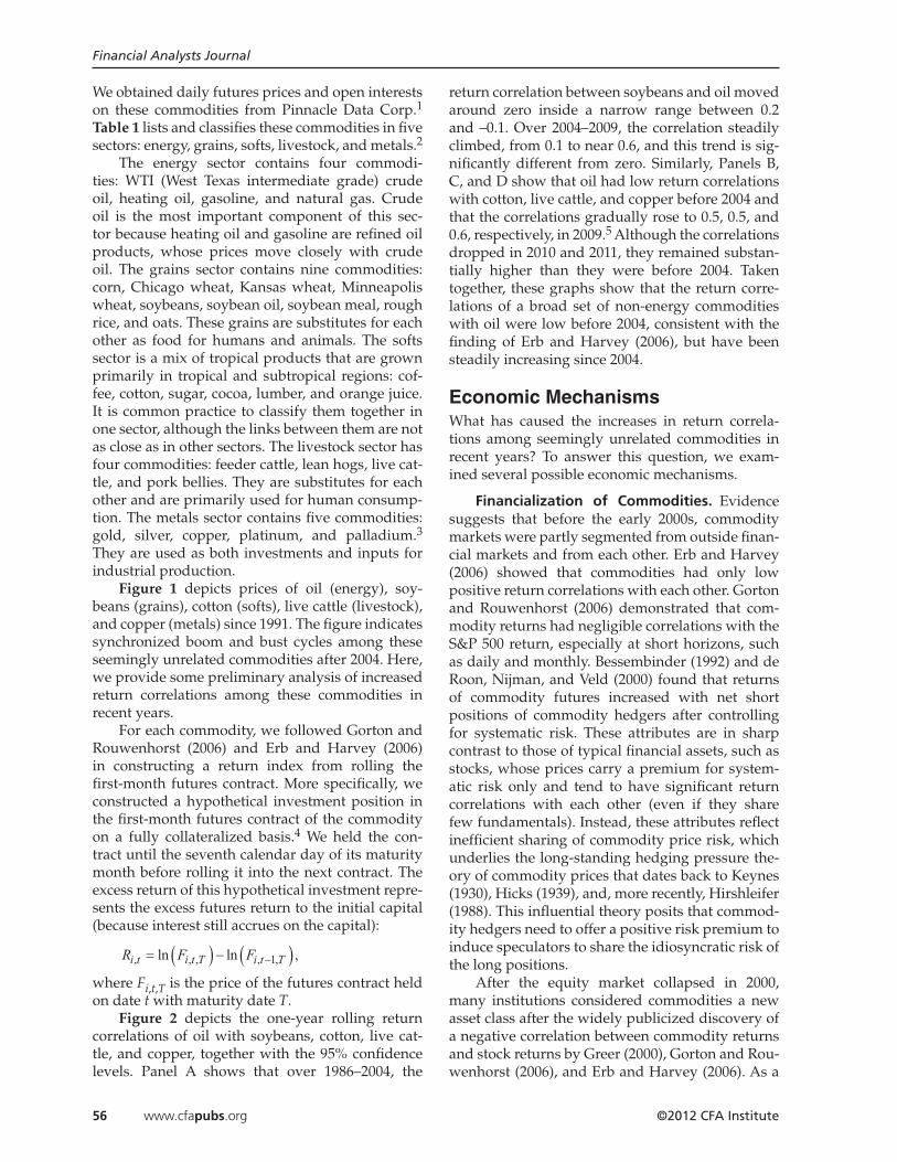
Figure 2 depicts the one-year rolling return correlations of oil with soybeans, cotton, live cat-tle, and copper, together with the 95% confidence levels. Panel A shows that over 1986–2004, the

return correlation between soybeans and oil moved around zero inside a narrow range between 0.2 and –0.1. Over 2004–2009, the correlation steadily climbed, from 0.1 to near 0.6, and this trend is sig-nificantly different from zero. Similarly, Panels B, C, and D show that oil had low return correlations with cotton, live cattle, and copper before 2004 and that the correlations gradually rose to 0.5, 0.5, and 0.6, respectively, in 2009.5 Although the correlations dropped in 2010 and 2011, they remained substan-tially higher than they were before 2004. Taken together, these graphs show that the return corre-lations of a broad set of non-energy commodities with oil were low before 2004, consistent with the finding of Erb and Harvey (2006), but have been steadily increasing since 2004.

Economic MechanismsWhat has caused the increases in return correla-tions among seemingly unrelated commodities in recent years? To answer this question, we exam-ined several possible economic mechanisms.

Financialization of Commodities. Evidence suggests that before the early 2000s, commodity markets were partly segmented from outside finan-cial markets and from each other. Erb and Harvey (2006) showed that commodities had only low positive return correlations with each other. Gorton and Rouwenhorst (2006) demonstrated that com-modity returns had negligible correlations with the S&P 500 return, especially at short horizons, such as daily and monthly. Bessembinder (1992) and de Roon, Nijman, and Veld (2000) found that returns of commodity futures increased with net short positions of commodity hedgers after controlling for systematic risk. These attributes are in sharp contrast to those of typical financial assets, such as stocks, whose prices carry a premium for system-atic risk only and tend to have significant return correlations with each other (even if they share few fundamentals). Instead, these attributes reflect inefficient sharing of commodity price risk, which underlies the long-standing hedging pressure the-ory of commodity prices that dates back to Keynes (1930), Hicks (1939), and, more recently, Hirshleifer (1988). This influential theory posits that commod-ity hedgers need to offer a positive risk premium to induce speculators to share the idiosyncratic risk of the long positions.

After the equity market collapsed in 2000, many institutions considered commodities a new asset class after the widely publicized discovery of a negative correlation between commodity returns and stock returns by Greer (2000), Gorton and Rou-wenhorst (2006), and Erb and Harvey (2006). As a



Table 1. Commodity Futures Traded in the United States and Weights in the S&P GSCI and DJ-UBSCI

CommodityS&PGSCI

DJ-UBSCI Exchangea Contract

Start of Futures in

U.S.

Start of Futures in

China

Energy

WTI crude oil 40.6% 15.0% NYMEX Every month 30/Mar/83

Heating oil 5.3 4.5 NYMEX Every month 14/Nov/78 25/Aug/04

RBOB gasoline 4.5 4.1 NYMEX Every month 18/Apr/06

Natural gas 7.6 16.0 NYMEX Every month 4/Apr/90

Grains

Corn 3.6% 6.9% CME Group Mar, May, Jul, Sep, Dec 1/Jul/59 22/Sep/04

Soybeans 0.9 7.4 CME Group Jan, Mar, May, Jul, Aug, Sep, Nov 1/Jul/59 4/Jan/99

Chicago wheat 3.0 3.4 CME Group Mar, May, Jul, Sep, Dec 1/Jul/59 4/Jan/99

Kansas wheat 0.7 0 KCBT Mar, May, Jul, Sep, Dec 5/Jan/70

Soybean oil 0 2.9 CME Group Jan, Mar, May, Jul, Aug, Sep, Oct, Dec 1/Jul/59

Minneapolis wheat 0 0 MGE Mar, May, Jul, Sep, Dec 5/Jan/70

Soybean meal 0 0 CME Group Jan, Mar, May, Jul, Aug, Sep, Oct, Dec 1/Jul/59

Rough rice 0 0 CME Group Jan, Mar, May, Jul, Sep, Nov 20/Aug/86

Oats 0 0 CME Group Mar, May, Jul, Sep, Dec 1/Jul/59

Softs

Coffee 0.5% 2.7% ICE Mar, May, Jul, Sep, Dec 16/Aug/72

Cotton 0.7 2.2 ICE Mar, May, Jul, Oct, Dec 1/Jul/59 1/Jun/04

Sugar 2.1 2.8 ICE Mar, May, Jul, Oct 4/Jan/61 6/Jan/06

Cocoa 0.2 0 ICE Mar, May, Jul, Sep, Dec 1/Jul/59

Lumber 0 0 CME Group Jan, Mar, May, Jul, Sep, Nov 1/Oct/69

Orange juice 0 0 ICE Jan, Mar, May, Jul, Sep, Nov 1/Feb/67

Livestock

Feeder cattle 0.3% 0% CME Group Jan, Mar, Apr, May, Aug, Sep, Oct 30/Nov/71

Lean hogsb 0.8 2.5 CME Group Feb, Apr, May, Jul, Aug, Oct, Dec 28/Feb/66

Live cattle 1.6 4.1 CME Group Feb, Apr, Jun, Aug, Oct, Dec 30/Nov/64

Pork bellies 0 0 CME Group Feb, Mar, May, Jul, Aug 18/Sep/61

Metals

Goldc 1.5% 6.1% NYMEX Feb, Apr, Jun, Aug, Oct, Dec 31/Dec/74 1/Jan/08

Silverc 0.2 2.4 NYMEX Jan, Mar, May, Jul, Sep, Dec 12/Jun/63

Copperd 2.6 6.7 NYMEX Mar, May, Jul, Sep, Dec 3/Jan/89 12/May/97

Platinumc 0 0 NYMEX Jan, Apr, Jul, Oct 4/Mar/68

Palladiumc 0 0 NYMEX Mar, Jun, Sep, Dec 3/Jan/77

Notes: This table lists all the commodities with futures contracts traded in the United States. The weights of these commodities in the S&P GSCI and DJ-UBSCI contracts are taken from 2008. The S&P GSCI and DJ-UBSCI also include commodities traded in London, which are not included in our analysis. aNYMEX represents the New York Mercantile Exchange. KCBT represents the Kansas City Board of Trade. MGE represents the Minneapolis Grain Exchange.bA June contract has been added to the lean hog futures series since 2002. Because this new contract has a low open interest, we omitted it from our analysis.cContracts include the current month and the next two consecutive months plus those contracts listed in the table. However, because the open interest of these short-maturity contracts (with maturities less than three months) is typically small, we omitted them from our analysis.dThe S&P GSCI uses copper contracts traded on the London Metal Exchange, whereas the DJ-UBSCI uses those from the NYMEX. We followed the convention of the DJ-UBSCI and chose March, May, July, September, and December for copper contracts.



result, billions of investment dollars flowed into commodity markets from financial institutions, insurance companies, pension funds, foundations, hedge funds, and wealthy individuals. The large index investment flow precipitated a fundamen-tal process of financialization among commodity markets—the focus of our analysis.

■ Commodity indices. The most popular com-modity investment strategy is to invest in a bas-ket of commodities in a given commodity index. A commodity index functions like an equity index, such as the S&P 500, in that its value is derived from the total value of a specified basket of commodities. Each commodity in the basket is assigned a partic-ular weight. Commodity indices typically build on the values of futures contracts, which are usually nearby contracts with delivery times longer than a month,6 to avoid the cost of holding physical com-modities. When a first-month contract matures and the second-month contract becomes the first-month contract, a commodity index specifies the so-called roll (i.e., replacing the current contract in the index with a following contract). In this way, commodity indices provide returns comparable to passive long positions in listed commodity futures contracts. By far the largest two indices by market share are the S&P GSCI and the DJ-UBSCI. These two indices use different selection and weighting schemes: the S&P GSCI is weighted by each com-modity’s world production, whereas the DJ-UBSCI relies on the relative amount of trading activity of

a particular commodity.7 Investors can use three types of financial instruments to gain exposure to the return of a commodity index: commodity index swaps, exchange-traded funds, and exchange-traded notes.8

Table 1 provides the weights of the 28 com-modities in the S&P GSCI and DJ-UBSCI in 2008. Both indices incorporate a wide range of commod-ity futures. Some commodities are in neither index: Minneapolis wheat, soybean meal, rough rice, and oats in the grains sector; lumber and orange juice in the softs sector; pork bellies in the livestock sec-tor; and platinum and palladium in the metals sec-tor. The composition of these indices has remained stable in recent years. Furthermore, the set of the S&P GSCI and DJ-UBSCI also covers almost all the commodities in other, less popular indices.

The energy sector carries a much greater weight than the other sectors in the S&P GSCI and DJ-UBSCI. The four energy commodities listed in Table 1 add up to 58% of the S&P GSCI and 39.6% of the DJ-UBSCI. WTI crude oil alone accounts for 40.6% of the S&P GSCI. Because the commodities in the energy sector move closely with each other, we used crude oil as a focal point in our analysis of the price comovements of non-energy commodities and oil.

■ Index investment flow. Each Friday, the CFTC releases a weekly Commitments of Traders report, which includes a Supplemental Commod-ity Index Trader (CIT) report. The CIT report shows the positions of a set of index traders identified

Figure 1. Commodity Futures Prices, January 1991–July 2011

Oil Soybeans Cotton Live Cattle Copper

Normalized Price (Jan/91 = 100)

500

100

50

96 02 06 08 109492 98 00 04

Notes: This figure depicts the futures prices of five commodities—oil, soybeans, cotton, live cattle, and copper. We normalized the price of each commodity in January 1991 to be 100 and used a logarithmic scale.



by the CFTC in 12 agricultural commodities since 3 January 2006. These commodities include corn, soybeans, Chicago wheat, Kansas wheat, and soy-bean oil in the grains sector; coffee, cotton, sugar, and cocoa in the softs sector; and feeder cattle, lean hogs, and live cattle in the livestock sector. This list coincides with the set of the S&P GSCI and DJ-UBSCI in these three sectors. The CIT report covers no commodities in the energy and metals sectors.

We can construct the investment flow from index traders in and out of the 12 commodities each week by summing the dollar values of their net position changes in these commodities:

IF NL NL Pt i t i t i ti

= −( )∑ − −=

, , , ,1 11

12 (1)

where NLi,t represents the net long position of index traders in commodity i in week t and Pi,t–1 is the price of the commodity in week t – 1. In this cal-culation, we use prices of first-month futures con-tracts and assume that all position changes occur during the previous week. Then, we can add the index flow from the first week of 2006 (the begin-ning of the CIT report data) to any week before 29 October 2009 to obtain the cumulated index flow up to that week.

Figure 2. Rolling Return Correlation of Oil with Various Non-Energy Commodities

Coefficient ρ 95% Confidence Level

CorrelationA. Soybean–Oil Pair

1.0

0.8

0.6

0.4

0.2

0

–0.2

–0.492 949088 96 98 00 02 04 06 08 10

CorrelationB. Cotton–Oil Pair

1.0

0.8

0.6

0.4

0.2

0

–0.2

–0.492 949088 96 98 00 02 04 06 08 10

CorrelationC. Live Cattle–Oil Pair

1.0

0.8

0.6

0.4

0.2

0

–0.2

–0.492 949088 96 98 00 02 04 06 08 10

CorrelationD. Copper–Oil Pair

1.0

0.8

0.6

0.4

0.2

0

–0.2

–0.492 9490 96 98 00 02 04 06 08 10

Notes: This figure depicts the one-year rolling return correlation of oil with soybeans, cotton, live cattle, and copper, together with the 95% confidence levels, in Panels A, B, C, and D, respectively. Panels A, B, and C start in 1986 because the trading of oil futures started only in March 1983. We omitted the data for 1983–1984 to avoid potential liquidity problems at the beginning and used returns after 1985 to measure correlations. With the one-year rolling window, our correlation measures start in 1986. Panel D starts in 1990 because the trading of copper futures started only in January 1989.



Figure 3 depicts the cumulated index flow, together with the S&P GSCI agriculture and live-stock excess return index, over January 2006–October 2009. This index follows the performance of the same three sectors—grains, softs, and livestock—that are covered by the CIT report. Fig-ure 3 shows that since the beginning of 2006, these three sectors have had a large net inflow, which cumulated to nearly $20 billion in early 2008. Then, an outflow led to a cumulated index flow of –$5 bil-lion by March 2009. The figure also shows that fluc-tuations of the S&P GSCI agriculture and livestock return index were in sync with the index flow. Our regression of the weekly commodity index return on the index flow also yielded a positive and signifi-cant coefficient. The significant correlation between the commodity return and the index flow does not represent causality, which can go from the index flow to the commodity return or vice versa.9 We exploited the difference between indexed and off-index commodities to identify the causality.10

■ Identification strategy. Index investors are not particularly sensitive to prices of individual commodities because they tend to move in and out of all commodities in a given index at the same time on the basis of the strategic allocation of their capital to commodities versus other asset classes, such as stocks and bonds. As a result, any shock to their strategic allocation to the commodity

class can cause commodities in the index to move together (see, e.g., Barberis and Shleifer 2003). In other words, we would expect price comovements of commodities in the S&P GSCI and DJ-UBSCI to be greater than those of off-index commodi-ties. Consistent with this theory, Barberis, Shleifer, and Wurgler (2005) found that in stock markets, a stock’s listing on the S&P 500 can significantly increase its return correlation with the index. Moti-vated by these studies, we exploited the difference between the return correlations of indexed and off-index commodities with oil to identify the increas-ing presence of index investors in the commodity markets. We chose oil as a focal point because of its dominant weight in the two most popular com-modity indices. In particular, we examined the fol-lowing empirical hypothesis regarding the change in this difference after 2004:

Hypothesis I. After 2004, non-energy commodities in the S&P GSCI and DJ-UBSCI had greater increases in return correlations with oil than did off-index commodities.

An implicit assumption in this hypothesis is that other participants in commodity markets, such as traditional speculators and commercial hedgers, have a limited capacity to absorb trades by index investors. As a result, the growing presence of index investors can affect commodity prices. Note also that potential substitutions between closely related commodities by consumers and producers

Figure 3. Cumulated Index Flow and S&P GSCI Agriculture and Livestock Excess Return Index, January 2006–October 2009

S&P GSCI Agriculture and Livestock Excess Return Index

S&P GSCI Agriculture and Livestock Excess Return Index

Cumulated Index Flow200

150

100

50

Index Flow ($ billions)

20

10

0

–1006 1007 08 09

Notes: This figure depicts the cumulated index flow to the 12 agricultural and livestock com-modities covered by the CFTC’s CIT report, together with the S&P GSCI agriculture and live-stock excess return index. We computed the weekly flow to each commodity according to Equa-tion 1 and the cumulated flow to each commodity by adding the weekly flow from the first week of 2006 to a given week. By summing the cumulated flows to the 12 commodities, we obtained the cumulated index flow.



can partly transmit the price impact of index inves-tors to off-index commodities.11 For example, if prices of corn rise far above those of soybean meal, consumers will substitute soybean meal for corn to feed their animals. Similarly, if prices of corn rise far above those of oats, farmers will allocate more farmland to corn than to oats. But these substitution effects are likely to be imperfect and to operate at horizons longer than those of futures trading, such as the daily horizon that we focused on in our study.

The choice of 2004 as the breakpoint is innocu-ous because our main results build on trends in return correlations between non-energy commodi-ties and oil. Our use of daily, rather than weekly or monthly, data allowed us to reliably measure changes in return volatility and correlation in the United States after 2004.

One might argue that trading by index inves-tors has a greater impact on commodities that carry a greater weight in the commodity indices. How-ever, because their index weights, by construction, are matched by their greater world production and higher trading liquidity in futures markets, we would expect these commodities to be able to absorb more capital inflow and outflow. Thus, we chose to focus on the difference in return correla-tions between commodities in and off the S&P GSCI and DJ-UBSCI, rather than between commodities with greater and lesser index weights.

Because the S&P GSCI and DJ-UBSCI are con-structed by rolling front-month futures contracts of individual commodities, we focused most of our analysis on the returns from rolling these front-month futures contracts. A subtle issue is whether the growth of index investment has affected spot prices in the same way, which depends on the effectiveness of arbitrageurs in synchronizing spot prices and futures prices. If the price of the front-month futures contract of a commodity becomes too expensive relative to its spot price—after adjusting for interest cost and storage cost for carrying the commodity from now until the contract’s delivery date—it becomes profitable for arbitrageurs to short the contract and simultaneously carry the commod-ity. Thus, we would expect arbitrageurs to spread the price impact of index investment from front-month futures contracts to spot prices if the interest cost and storage cost incurred in such carry trades are independent of growing index investment. We also examined the correlations of spot returns.

Rapid Growth of Emerging Economies. The rapid growth of China, India, and other emerging economies is a popular explanation for the recent commodity price boom (see, e.g., Krugman 2008; Hamilton 2009; Kilian 2009). The development of these emerging economies in the past decade stim-

ulated unprecedented demands for a broad range of commodities in various sectors, such as energy and metals, and thus may have led to a joint price boom for these commodities.

The commodity demands from the emerg-ing economies depend positively on the strength of their economic growth and negatively on the price of the U.S. dollar, which is widely used to settle commodity transactions. We used the MSCI Emerging Markets Index to proxy for the growth of emerging economies. We also used the return of the U.S. Dollar Index futures traded on ICE (IntercontinentalExchange) to track price fluctua-tions of the U.S. dollar. Underlying this futures contract is an index that weights dollar exchange rates with six currencies (euro, Japanese yen, Brit-ish pound, Canadian dollar, Swedish krona, and Swiss franc). We obtained data on these two indi-ces from Bloomberg.

Figure 4 depicts the one-year rolling correla-tion between daily returns of the S&P GSCI and the MSCI Emerging Markets Index. Before 2004, the correlation fluctuated, mostly around zero, except that it dropped to –0.4 during the Gulf War in 1990–1992. The war caused stock prices to fall and oil prices to soar. Interestingly, after 2004, the cor-relation rose gradually, from around 0 to above 0.5 after 2009. This rising trend is consistent with the increasingly important effects of emerging econo-mies on commodity prices in recent years. Figure 4 also shows a clear decreasing trend in return cor-relations between the S&P GSCI and the U.S. Dollar Index. Before 2004, this correlation fluctuated inside a narrow band between –0.2 and 0.2. After 2004, it dropped steadily, from around 0 to below –0.4 after 2009. This trend is consistent with both growing commodity demands from emerging economies and increasing commodity index investment from outside the United States. In our regression analysis of price comovements of non-energy commodities and oil, we used the MSCI Emerging Markets Index and the U.S. Dollar Index to control for the effects of commodity demands from emerging economies.

Despite the important effects of emerging economies on commodity prices, it remains unclear whether they have driven the increased price cor-relations across the broad range of commodities since 2004. To address this question, we collected futures prices of commodities traded in China, the growth engine of emerging economies in the past decade, from Wind (a widely used vendor of finan-cial data in China). China has been gradually intro-ducing futures contracts on a set of commodities since the late 1990s. Table 1 lists these commodities and the starting dates of futures trading in China. Figure 5 depicts front-month futures prices for six



commodities in China and the United States.12 Panels A, B, and C show that futures prices of heat-ing oil, copper, and soybeans in China had boom-and-bust cycles closely matched by corresponding cycles in the United States. These closely matched price dynamics are consistent with the rapidly growing imports of these commodities by China in recent years (Commodity Research Bureau 2009). More interestingly, Panels D, E, and F show that the prices of wheat, corn, and cotton in China did not display any pronounced cycle around 2008, in sharp contrast to the boom-and-bust cycles experienced by the prices of these commodities in the United States. Because China is not a major importer or exporter of wheat, corn, and cotton (Commodity Research Bureau 2009), this contrast is perhaps not so surprising.13 Nevertheless, it raises doubt that commodity demands from China are the driver of all commodity prices in the United States.

We also compared the average commodity return correlations in China and the United States in a sample of eight commodities with futures contracts simultaneously traded in China and the United States.14 Interestingly, the average com-modity return correlation in China did not experi-ence the same dramatic increase as in the United States after 2004. This contrast again refutes com-modity demands from China as the driver of the large increases in commodity price comovements in the United States.

The World Financial Crisis. It is well known that prices of financial assets tend to move together during financial crises. Could the recent increases in commodity return correlations be simple reflec-tions of the recent financial crisis? The crisis erupted in full only after the failure of Lehman Brothers, in September 2008. The timing of the crisis did not coincide with the increases in commodity return correlations, which started in 2004—long before September 2008. Thus, the financial crisis cannot fully explain the increases in commodity return correlations. In our regression analysis (discussed later in the article), we treated separately the pre-crisis period before September 2008 to isolate the crisis effect.

Inflation. Inflation is a common factor that drives prices of various commodities. Could the recent rise in commodity return correlations be driven by an increasingly important effect of infla-tion on commodity prices?

Figure 6 depicts the annualized monthly core inflation rate of the U.S. Consumer Price Index (the percentage change of the CPI excluding food and energy prices) and the one-year rolling volatility of the monthly CPI core inflation rate. We used the CPI core inflation rate to avoid the contamination of the inflation measure by commodity prices. This infla-tion rate hovered near 10% throughout the 1970s, when the economy was hit by persistent oil supply

Figure 4. Rolling Return Correlations of the S&P GSCI with the MSCI Emerging Markets Index (January 1989–July 2011) and the U.S. Dollar Index (January 1987–July 2011)


Correlation

A. S&P GSCI and MSCI Emerging Markets Index

0.8

0.6

0.4

0.2

0

–0.4

–0.2

–0.692 9490 96 98 00 02 04 06 08 10

Correlation

B. S&P GSCI and U.S. Dollar Index

0.6

0.4

0.2

–0.4

–0.2

0

–0.6

–0.8929088 94 96 98 00 02 04 06 08 10

Note: This figure depicts the one-year rolling return correlations of the S&P GSCI excess return index with the MSCI Emerging Markets Index in Panel A and with the U.S. Dollar Index in Panel B.



shocks and stagflation. The inflation rate remained high—around 5%—during the 1980s. Inflation was eventually tamed in the 1990s and remained low, at 2–3%, throughout the late 1990s and the past decade. The volatility of the inflation rate has a pat-tern similar to that of the inflation rate’s monthly measure. It was often above 5% in the 1970s and early 1980s and remained above 3% from the early 1980s to the early 1990s. After the mid-1990s, infla-tion volatility gradually declined, reaching about 1% in the early 2000s, and it remained at that level

over the past decade. Interestingly, the commod-ity return correlations depicted in Figure 2 show time trends opposite to those of the inflation rate and inflation volatility over the past decade. Thus, it is unlikely that the recent increases in commodity return correlations were driven by inflation.

Adoption of Biofuel. Another recent devel-opment in commodity markets is the wide adop-tion of biofuel. To reduce the reliance on oil as the main source of energy, many countries, including

Figure 5. Normalized Commodity Prices in China and the United States

PriceA. Heating Oil

300

250

200

150

100

500605 07 08 09 10 11

PriceB. Copper

400

300

200

100

00605040302010099989796 07 08 09 10 11

PriceC. Soybeans

350

250

300

200

150

100

500605040302010099 07 08 09 10 11

PriceD. Wheat

500

300

200

400

100

00605040302010099 07 08 09 10 11

PriceE. Corn

400

300

200

100

00605 07 08 09 10 11

PriceF. Cotton

400

300

200

100

00605 07 08 09 10 11

U.S. Price Chinese Price

Notes: This figure depicts the front-month futures prices of six commodities—heating oil, copper, soybeans, wheat, corn, and cotton—in China and the United States. The prices in China are settled in renminbi. Each price series is normalized to 100 in its own currency at the beginning of its sample period.



the United States, have adopted new energy policies to promote the use of biofuel. In the United States, the Energy Policy Act of 2005 man-dated that 7.5 billion gallons of ethanol be used by 2012; the Energy Independence and Security Act of 2007 increased the mandate to 36 billion by 2022. The combination of ethanol subsidies and high oil prices led to a rapid growth of the ethanol industry, which now consumes about one-third of U.S. corn production. The rise of the ethanol industry might have caused prices of corn and such close substitutes as soybeans and wheat to comove with oil prices. Because corn is a major source of livestock feed, this effect may also have influenced prices of livestock commodi-ties. However, the growth of ethanol production can explain neither the synchronized price booms of commodities unrelated to food, such as cot-ton and coffee, nor the greater increase in return correlations among indexed commodities than among off-index commodities.15

Regression AnalysisWe used regression analysis to examine our main hypothesis—Hypothesis I—by controlling for the other effects discussed previously.

Average Return Correlations of Indexed and Off-Index Commodities. We first plotted the aver-age return correlations among indexed and off-index commodities going back to the 1970s. We constructed an average return correlation for all commodities with futures contracts traded at a given time. Because commodities in the same sector tend to have greater return correlations with each other than with commodities in other sectors, we had to avoid the potential bias caused by changes in commodity distribution across sec-tors. We dealt with this issue by using the follow-ing method: For each sector, we constructed an index that tracks the equal-weighted return of all available commodities. Then, we computed the return correlations between these indices for all sector pairs and took the equal-weighted aver-age. To highlight the difference between com-modities in and off the two popular commod-ity indices, we constructed two separate return indices for indexed and off-index commodities in each sector and calculated the average correla-tions of indexed and off-index commodities. We called a commodity “indexed” if it was in either the S&P GSCI or the DJ-UBSCI and “off-index” otherwise.

Figure 6. Inflation and Inflation Volatility, January 1970–July 2011

Inflation

Inflation

Inflation Volatility

0.2

0.1

0

Inflation Volatility

0.10

0.05

070 908575 9580 00 05 10

Note: This figure depicts the annualized monthly CPI core inflation rate (excluding food and energy prices) and the one-year rolling volatility of the monthly CPI core inflation rate.



Figure 7 depicts the average one-year rolling cor-relations of indexed and off-index commodities over 1973–2011. The figure illustrates several interesting points. The average correlation among indexed com-modities stayed at a stable level, below 0.1, through-out the 1990s and early 2000s and was indistinguish-able from that among off-index commodities. In 2009, the mild increase in average correlation among off-index commodities, to 0.2, was in sharp contrast to that among indexed commodities, which climbed to an unprecedented level of more than 0.5. This difference in the increase in correlations between indexed and off-index commodities is consistent with the effect of index investment discussed previ-ously. Although the correlations among both indexed and off-index commodities have dropped since 2010, a substantial difference nevertheless exists between indexed and off-index commodities.

Figure 7 also shows that the average correlations of indexed and off-index commodities were as high as 0.3 in the 1970s. As we discuss later in the arti-cle, these high correlations coincided with the wild inflation and inflation volatility during that period. The average correlations gradually declined, to below 0.1 in the late 1980s, as inflation and inflation volatility were eventually tamed. Interestingly, there were no pronounced differences between indexed

and off-index commodities despite the high correla-tion levels in the 1970s. This contrast between the high return correlations of the 1970s and those of the past decade indicates that they were driven by different mechanisms. We focused our analysis on understanding the latter period.

Price Comovements of Non-Energy Commod-ities with Oil. In formally testing Hypothesis I by using regression analysis, we pooled daily returns of first-month futures contracts of all non-energy commodities from 2 January 1998 to 15 July 2011. We chose this sample period so that there would be six years before 1 January 2004 and roughly seven years afterward. As we discussed previously, there is not much difference between the return correla-tions of indexed and off-index commodities in the earlier period. Extending the sample period further back does not affect our result.

We normalized the daily return of commodity i by its average return and return volatility:

RR R

Ri tn i t i

i,

, .=− ( )

( )mean

std

We specified the following panel regression of the normalized commodity return ( ),Ri t

n on the normalized oil return ( ),Roil t

n and a set of control

Figure 7. Average Correlations of Indexed and Off-Index Commodities, 1973–2011

Average Correlation of Indexed Commodities

Average Correlation of Off-Index Commodities

Correlation

0.6

0.5

0.4

0.3

0.2

0.1

0

–0.185 908075 95 00 05 10

Notes: This figure depicts the average return correlations of commodities in the S&P GSCI and DJ-UBSCI and commodities off these indices. We separated the samples of indexed and off-index commodities. In each sample, we constructed an equal-weighted return index for each commodity sector. A commodity is not included in the index until its aver-age daily futures trading volume in a given calendar year is larger than $20 million. Then, for both indexed and off-index commodities, we computed the equal-weighted averages of the one-year rolling return correlations of all sector pairs.



variables comprising the normalized returns of the MSCI Emerging Markets Index ( ),,REM t

n the S&P 500 ( ),,RSP t

n the J.P. Morgan U.S. Aggregate Bond Index ( ),,RJPM t

n and the U.S. Dollar Index ( ),RUSD tn :

Rt I

t I Ii tn i t

t index, = +

+ −( )+ −( )⎡

⎣⎢⎢

⎤≥

≥α

β β

β0 1 2004

2 2004

2004

2004 ⎦⎦⎥⎥

++ −( )

+ −( )⎡ ≥

≥

R

t I

t I I

oil tn

i t

t index

,

κ κ

κ0 1 2004

2 2004

2004

2004⎣⎣⎢⎢

⎤

⎦⎥⎥

++ −( )

+ −( )≥

≥

R

t I

t I I

EM tn

i t

t ind

,

γ γ

γ0 1 2004

2 2004

2004

2004 eexSP tn

i t

t

R

t I

t I I

⎡

⎣⎢⎢

⎤

⎦⎥⎥

++ −( )

+ −( )≥

≥

,

θ θ

θ0 1 2004

2 2004

2004

2004 iindexJPM tn

i t

t

R

t I

t I

⎡

⎣⎢⎢

⎤

⎦⎥⎥

++ −( )

+ −( )≥

≥

,

η η

η0 1 2004

2 2

2004

2004 0004IR

indexUSD tn⎡

⎣⎢⎢

⎤

⎦⎥⎥

+

(2)

Iindex is an indicator function with a value of 1 if the commodity is in either the S&P GSCI or the DJ-UBSCI and zero otherwise. We included returns of the MSCI Emerging Markets Index and the U.S. Dollar Index to control for the effect of commodity demands from emerging economies. Because the dollar return should also pick up the effects of inter-national index investors, this control might be exces-sive. We also included returns of the S&P 500 and the J.P. Morgan U.S. Aggregate Bond Index to control for the effects of the macroeconomic fundamentals.

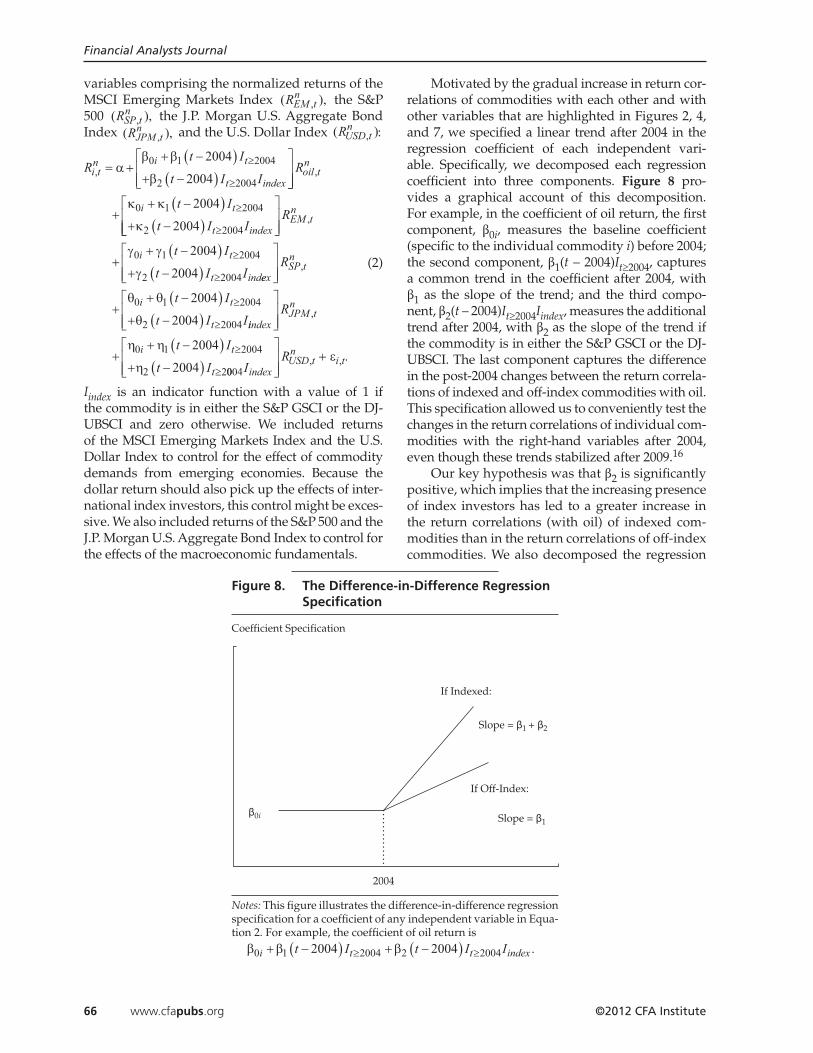
Motivated by the gradual increase in return cor-relations of commodities with each other and with other variables that are highlighted in Figures 2, 4, and 7, we specified a linear trend after 2004 in the regression coefficient of each independent vari-able. Specifically, we decomposed each regression coefficient into three components. Figure 8 pro-vides a graphical account of this decomposition. For example, in the coefficient of oil return, the first component, β0i, measures the baseline coefficient (specific to the individual commodity i) before 2004; the second component, β1(t – 2004)It 2004, captures a common trend in the coefficient after 2004, with β1 as the slope of the trend; and the third compo-nent, β2(t – 2004)It 2004Iindex, measures the additional trend after 2004, with β2 as the slope of the trend if the commodity is in either the S&P GSCI or the DJ-UBSCI. The last component captures the difference in the post-2004 changes between the return correla-tions of indexed and off-index commodities with oil. This specification allowed us to conveniently test the changes in the return correlations of individual com-modities with the right-hand variables after 2004, even though these trends stabilized after 2009.16

Our key hypothesis was that β2 is significantly positive, which implies that the increasing presence of index investors has led to a greater increase in the return correlations (with oil) of indexed com-modities than in the return correlations of off-index commodities. We also decomposed the regression

Figure 8. The Difference-in-Difference Regression Specification

Coefficient Specification

2004

If Indexed:

If Off-Index:

Slope = β1β0i

Slope = β1 + β2

Notes: This figure illustrates the difference-in-difference regression specification for a coefficient of any independent variable in Equa-tion 2. For example, the coefficient of oil return is β β β0 1 2004 2 20042004 2004i t t indext I t I I+ −( ) + −( )≥ ≥ .



coefficient of each of the control variables in the same way to control for possible trends driven by other economic mechanisms.

We analyzed this regression in the full sample with all non-energy commodities, as well as in sev-eral subsamples that included the soybean complex (which contains soybeans, soybean meal, and soy-bean oil), the grains sector, the softs sector, the live-stock sector, and the metals sector. We examined separately the pre-crisis period, from 2 January 1998 to 31 August 2008, and the full sample period, from 2 January 1998 to 15 July 2011, in order to iso-late the crisis effect. For each of the periods, we ana-lyzed the regression first with only oil return and then together with the control variables. Table 2 reports the regression results.

Panel A reports the results from the full sam-ple, with all non-energy commodities. The esti-mates of β1 and β2 in both the pre-crisis and the full sample periods are positive and significant. These estimates suggest that after 2004, there was a sig-nificant and increasing trend in return correlations of non-energy commodities with oil. More impor-tantly, this increasing trend is significantly stronger for indexed commodities than for off-index com-modities. This pattern is robust to including the control variables in the regressions and thus sup-ports Hypothesis I—that is, the increasing presence of index investors led prices of indexed commodi-ties to comove more with oil. Furthermore, this effect was present even before the disruptions of the financial crisis in September 2008.

In the pre-crisis period with the control vari-ables, the estimates of β1 and β2 are 0.04 and 0.02, respectively. The former value suggests that the return correlation between an off-index non-energy commodity and oil increased by 0.04 each year. At that rate, the correlation had a cumulative increase of 0.28 over 2004–2011. The return correlation between an indexed non-energy commodity and oil had an extra increase of 0.02 each year. Thus, its cumulative increase over 2004–2011 was 0.42, which is substantial in economic terms.

Panel B of Table 2 also reports the estimates of β1 and β2 in each subsample of non-energy com-modities after including the control variables. The estimates are consistently positive and significant across the subsamples except in the livestock sec-tor, in which the estimate of β1 is zero and the esti-mate of β2 is positive (but significant only in the full sample period). Taken together, the increased price comovements of indexed non-energy commodities and oil were not driven by a few commodities con-centrated in one sector; rather, our result regarding the increased price comovements is robust across various subsamples of commodities.17

Panel A of Table 2 also reveals several inter-esting observations about the return correlations of non-energy commodities with the control vari-ables. First, there is a significant and positive trend in their return correlations with the MSCI Emerg-ing Markets Index after 2004 in both the pre-crisis and the full sample periods, as reflected by the positive and significant estimates of coefficient κ1. This finding is consistent with the increasing return correlation between the S&P GSCI and the MSCI Emerging Markets Index after 2004. However, the estimates of κ2—the difference between indexed and off-index commodities in the increase of their return correlations with the MSCI Emerging Mar-kets Index—are small and insignificant in the pre-crisis period and even negative in the full sample period. This lack of difference is consistent with the fact that the effects of commodity demands from emerging economies are independent of the com-modity indices. It also indirectly confirms the dis-criminating power of our identification strategy based on the difference-in-difference effect.

Furthermore, the estimates of coefficient η1 are negative, with a significant t-statistic in the full sample period and an insignificant one in the pre-crisis period. These estimates suggest a negative trend in the return correlations of non-energy com-modities with the U.S. dollar after 2004, which is consistent with the decreasing trend in the return correlation between the S&P GSCI and the U.S. Dollar Index. More interestingly, the estimates of coefficient η2 are also negative, with a significant t-statistic in the pre-crisis period and an insignifi-cant one in the full sample period. These estimates indicate that the decreasing trend is stronger for indexed commodities than for off-index commodi-ties. This difference-in-difference result suggests that the decreasing trend in return correlations of non-energy commodities with the U.S. dollar was not driven entirely by commodity demands from emerging economies and was at least partly related to trading by international index investors in com-modity markets.

As mentioned earlier, commodities in the S&P GSCI and DJ-UBSCI are selected on the basis of their world production and trading liquidity in futures markets. Hence, the higher liquidity of indexed commodities works against our hypothesis because prices of more liquid commodities are less likely to be affected by the trading of index investors. Liquid-ity might be a concern for off-index commodities because it can cause price fluctuations of off-index commodities to lag behind oil. To account for this concern, we also introduced two lags of the oil return in the regression analysis. These unreported results show that the difference-in-difference effect



Table 2. Regressions of Daily Futures Returns of Non-Energy Commodities

Pre-Crisis Period (2 January 1998–31 August 2008)

Full Sample Period (2 January 1998–15 July 2011)

Estimate t-Stat. Estimate t-Stat. Estimate t-Stat. Estimate t-Stat.

A. Full sample, with all non-energy commodities

Trend with oil after 2004

β1 0.6 10.48 0.04 8.21 0.05 18.27 0.03 10.04

β2 0.2 3.55 0.02 2.61 0.02 5.26 0.02 4.91

Trend with MSCI Emerging Markets Index after 2004

κ1 0.02 4.41 0.02 6.32

κ2 0.00 –0.39 –0.01 –2.69

Trend with S&P 500 after 2004

γ1 –0.01 –1.09 –0.01 –2.08

γ2 0.00 0.27 0.00 0.80

Trend with J.P. Morgan U.S. Aggregate Bond Index after 2004

θ1 –0.01 –1.48 0.00 –0.93

θ2 –0.01 –0.91 0.00 0.13

Trend with U.S. Dollar Index after 2004

η1 –0.01 –1.10 –0.01 –2.75

η2 –0.02 –2.47 0.00 –0.23

R2 2.13% 4.64% 5.57% 8.98%

B. Estimates of β1 and β2 in various commodity sectors

Soybean complex

β1 0.07 4.29 0.04 4.48

β2 0.06 2.90 0.04 3.57

Grains sector

β1 0.06 6.84 0.04 8.97

β2 0.04 3.21 0.02 4.00

Softs sector

β1 0.02 2.07 0.01 2.42

β2 0.02 1.56 0.02 2.71

Livestock sector

β1 0.00 0.26 0.00 –0.34

β2 0.01 0.35 0.03 3.31

Metals sector

β1 0.05 5.42 0.04 6.15

β2 0.03 2.08 0.02 2.30

Notes: This table reports results from the regression specified in Equation 2. We adjusted the t-statistics for heteroscedasticity and serial correlation by using the Newey–West method with five lags. Panel A reports regression results for the full sample, with all non-energy commodities. To save space, we omitted the estimates for α, β0i, κ0i, γ0i, θ0i, and η0i in Panel A. Panel B separately reports the estimates of the main variables of interest, β1 and β2, in various subsamples of commodities.



between the return correlations of indexed and off-index commodities with oil is robust to the illiquid-ity concern.18

Spot Returns. Thus far, our analysis has focused on returns of rolling front-month futures contracts of various commodities. Does the difference-in-difference effect also hold for spot returns? We analyzed the spot return correlations of non-energy commodities with oil. Owing to the lack of centralized spot markets for commodi-ties, spot prices are often not readily available. We acquired spot prices for a set of commodities from Pinnacle Data Corp. The set includes oil and 16 non-energy commodities (8 short of the non-energy commodities with futures listed in Table 1). These non-energy commodities include corn, soybeans, wheat, Kansas wheat, soybean oil, Minneapolis wheat, and oats from the grains sector; cotton and sugar from the softs sector; live cattle and lean hogs from the livestock sector; and gold, silver, copper, platinum, and palladium from the metals sector.

We pooled their daily spot returns and regressed them on the spot return of oil and the set of control variables based on the regression speci-fied in Equation 2. The estimates of coefficients β1 and β2 are reported in Table 3. The estimate of β1 is positive and significant in the pre-crisis period but is insignificant in the full sample period. More interestingly, the estimate of β2 is positive and sig-nificant in both the pre-crisis period and the full sample period, confirming the same difference-in-difference effect in spot returns as in returns of rolling front-month futures contracts. This result implies that the price effect generated by the grow-ing commodity index investment in recent years is also present in spot prices of commodities.

Volatility SpilloverThe trading of index investors can act as a chan-nel to spill volatility from outside financial markets on and across commodity markets. We examined this spillover effect. Figure 9 depicts the annual-ized daily return volatility of oil, the S&P GSCI non-energy excess return index, and the S&P 500

estimated from one-year rolling windows. The S&P GSCI non-energy excess return index tracks price fluctuations of S&P GSCI commodities in the four non-energy sectors. Figure 9 shows that the price of oil is always volatile. During most of the 1990s and the past decade, its volatility was at least twice as high as the volatility of the S&P 500. In 2008, oil return volatility shot up from around 30% to 60%, a level that caused great public concern. However, oil return volatility had also reached this level before—in the early 1990s, during the Gulf War. More importantly, although the return volatility of non-energy commodities was stable—around 10%—throughout the 1990s and early 2000s, it started to rise after 2004 and peaked at an unprec-edented 27% in 2008, concurrent with the hikes in volatility of oil and the S&P 500.

Various factors may have contributed to the large volatility increase in oil and non-energy commodities. First, the world economic recession that accompanied the recent financial crisis made macroeconomic fundamentals more uncertain and thus commodity demands and prices more volatile. Second, the financial crisis, which initially disrupted the markets for mortgage-backed securi-ties, eroded the balance sheets of many financial institutions and eventually reduced the risk appe-tite of financial investors (including index inves-tors) for seemingly unrelated assets in their port-folios, including commodities (see, e.g., Kyle and Xiong 2001).

Figure 10 depicts the one-year rolling corre-lation between the S&P GSCI and the S&P 500. It illustrates a widely noted correlation increase: Although this correlation stayed in a band between –0.2 and 0.1 for several years before 2008, it quickly climbed from 0 to around 0.6 during the crisis and remained high even after the crisis abated, in early 2009. This largely increased cor-relation is consistent with both increased macro-economic uncertainty and the potential spillover of index investors.

To identify the spillover effect of index inves-tors, we analyzed the difference in return volatil-ity between indexed and off-index non-energy

Table 3. Regression Analysis of Spot Returns

Pre-Crisis Period (2 January 1998–31 August 2008)

Full Sample Period (2 January 1998–15 July 2011)

Estimate t-Stat. Estimate t-Stat.

β1 0.03 2.83 0.00 0.26

β2 0.03 2.96 0.03 4.37

Notes: This table reports the regression results of daily spot returns and only the coefficients related to the trends with oil after 2004. We adjusted the t-statistics for heteroscedasticity and serial correlation by using the Newey–West method with five lags.



commodities from 2 January 1998 to 15 July 2011. We first normalized the daily return of each commodity (the return of rolling its first-month futures contract) by its pre-2004 volatility and its whole sample mean. After the normalization, the return series of all non-energy commodities

have the same volatility before 2004. We then ana-lyzed changes in volatilities after 2004 by regress-ing the pooled, squared, normalized returns on a set of year dummies for each year after 2004 and their interaction terms with an index dummy for whether a given commodity is in either the S&P GSCI or the DJ-UBSCI:

R a b I b I b I

b I b Ii tn

i y y y

y y

,( ) = + + +

+ + +

= = =

= =

20 04 04 05 05 06 06

07 07 08 08 bb I b I

b I c I I c I Iy y

y index y index y

09 09 10 10

11 11 04 04 05 05

= =

= = =

+

+ + +

+ cc I I c I I

c I I c I Iindex y index y

index y index y

06 06 07 07

08 08 09

= =

= =

+

+ + 009

10 10 11 11+ + += =c I I c I Iindex y index y i tε , .

(3)

The squared return is a convenient and widely used measure of return volatility (see, e.g., Ander-sen, Bollerslev, Diebold, and Ebens 2001). The coefficients b04, b05, b06, b07, b08, b09, b10, and b11 measure the baseline volatility changes of off-index commodities in each of the years after 2004, whereas the coefficients c04, c05, c06, c07, c08, c09, c10, and c11 measure the additional volatility increase of indexed commodities relative to off-index com-modities in each of the years. Table 4 reports the regression results. It shows that the estimates of b08, b09, b10, and b11 are positive and significant, indicating a significant baseline volatility increase

Figure 9. Volatility of Oil, the S&P GSCI Non-Energy Excess Return Index, and the S&P 500, January 1989–July 2011

Oil S&P 500 S&P GSCI Non-Energy Excess Return Index

Volatility

0.8

0.7

0.6

0.5

0.4

0.3

0.2

0.1

094 00 0692 98 04 100890 96 02

Note: This figure depicts the one-year rolling volatility of the daily returns of oil, the S&P GSCI non-energy excess return index, and the S&P 500.

Figure 10. Return Correlation between the S&P GSCI and the S&P 500, January 1990–July 2011


Correlation

0.8

0.6

0.4

0.2

–0.2

0

–0.4

–0.692 9490 96 98 00 02 04 06 08 10

Note: This figure depicts the one-year rolling correlation of daily returns of the S&P GSCI and the S&P 500.



in 2008 and 2009 across the commodities. Inter-estingly, the estimates of c04, c06, c07, c08, c09, and c11 are all positive and significant, indicating that indexed commodities exhibited larger volatility increases than did off-index commodities in 2004, 2006, 2007, 2008, 2009, and 2011. This result is con-sistent with a spillover effect by commodity index investors.

The greater volatility increases of indexed com-modities may be due to their greater exposures to uncertainty about the economy, turmoil in stock markets and bond markets, or shocks to oil prices. Following our earlier analysis, we highlighted the contribution by the greater correlations of indexed commodities with oil. From each non-energy com-modity return, we used a two-step procedure to filter out fluctuation related to other variables. We first filtered out a set of control variables (MSCI Emerging Markets Index returns, S&P 500 returns, J.P. Morgan U.S. Aggregate Bond Index returns, U.S. Dollar Index returns, and the CPI core infla-tion rate) and then filtered out oil returns by using the following regression:

R a a I b b I t R

c c I tit t t EM t

t

= + + + −( )⎡⎣ ⎤⎦+ + −

≥ ≥

≥

0 1 04 0 1 04

0 1 04

2004

200,

44

2004

2000 1 04

0 1 04

( )⎡⎣ ⎤⎦+ + −( )⎡⎣ ⎤⎦+ + −

≥

≥

R

d d I t R

e e I t

SP t

t JPM t

t

,

,

44

2004

200 1 04

0 1 04

( )⎡⎣ ⎤⎦+ + −( )⎡⎣ ⎤⎦+ + −

≥

≥

R

f f I t R

h h I t

USD t

t CPI t

t

,

,

004( )⎡⎣ ⎤⎦ +Roil t t, .ε

(4)

Because we had only monthly observations for the CPI inflation rate, we treated RCPI,t as con-stant during a month. Depending on whether we included oil return in the regression, we obtained two sets of residual returns—one after filtering out only the control variables and the other after filter-ing out the control variables and oil return. The control variables served to filter out the potential effects of macroeconomic uncertainty, as well as possible spillover of stock market volatility and U.S. dollar volatility to commodities. Using these controls, we obtained estimates of the spillover of oil price volatility to indexed non-energy commod-ities, with the caveat that there might be unidenti-

Table 4. Regression Analysis of Volatility of Non-Energy Commodities

Raw ReturnsResidual Returns after

Control VariablesResidual Returns after Control

Variables and Oil Return

Estimate t-Stat. Estimate t-Stat. Estimate t-Stat.

A. Baseline effects

b04 0.25 3.50 0.20 2.87 0.20 2.88

b05 –0.09 –1.62 –0.12 –2.11 –0.12 –2.22

b06 –0.01 –0.16 –0.08 –1.32 –0.09 –1.54

b07 –0.07 –1.18 –0.12 –2.11 –0.13 –2.25

b08 1.45 10.85 1.09 9.56 0.97 8.91

b09 0.67 8.54 0.48 6.64 0.44 6.38

b10 0.39 4.14 0.25 2.85 0.23 2.68

b11 0.29 3.08 0.13 1.49 0.09 1.08

B. Difference-in-difference effects

c04 0.34 3.53 0.26 2.83 0.25 2.72

c05 0.09 1.25 0.07 1.06 0.06 0.91

c06 0.54 4.63 0.45 4.48 0.39 4.10

c07 0.25 3.39 0.16 2.31 0.13 1.90

c08 0.68 3.41 0.41 2.47 0.23 1.53

c09 0.33 2.93 0.18 1.78 0.10 1.08

c10 0.06 0.53 0.06 0.63 0.04 0.35

c11 0.46 3.32 0.42 3.42 0.33 2.99

R2 4.25% 3.08% 2.62%

Notes: This table reports the regression analysis of the volatility of non-energy commodities from 2 January 1998 to 15 July 2011. To save space, we report only the estimates of coefficients related to changes in volatility after 2004. We adjusted the t-statistics for heteroscedasticity and serial correlation by using the Newey–West method with five lags.



fied shocks that simultaneously affect the prices of oil and non-energy commodities.

We then repeated the difference-in-difference analysis of Equation 3 by using the two sets of residual returns. The results are reported in Table 4. After filtering out only the control variables from non-energy commodity returns, we found that the estimates of coefficients c04, c06, c07, c08, c09, and c11 are substantially reduced, although c04, c06, c07, c08, and c11 are still positive and significant. After filter-ing out oil return, we found that estimates of these coefficients are further reduced and the estimates of c07 and c08 are insignificant. These reductions indi-cate that the spillover of oil price volatility through index investment contributed to the greater volatil-ity increase of indexed non-energy commodities in 2007 and 2008.

Overall, we found that non-energy commodi-ties in the S&P GSCI and DJ-UBSCI had significantly greater volatility increases than did off-index com-modities in 2008. In particular, the greater volatility increases of indexed commodities were related to their greater return correlations with oil. These results are consistent with the hypothesis that trading by commodity index investors can act as a channel for spilling price volatility on commodity markets.

ConclusionIn our study, we found that, concurrent with the rapid growth of index investment in commodity markets, prices of non-energy commodities have become increasingly correlated with oil prices. This trend is significantly more pronounced for com-modities in two popular indices: the S&P GSCI and the DJ-UBSCI. Our findings reflect a fundamental process of financialization among commodity mar-kets, through which commodity prices have become more correlated with each other. As a result of the financialization process, the price of an individual commodity is no longer determined solely by its supply and demand. Instead, prices are also deter-mined by the aggregate risk appetite for financial assets and the investment behavior of diversified commodity index investors. This fundamental change, which is likely to persist so long as com-modity index investment remains popular among financial investors, has profound implications for a wide range of issues, including commodity produc-ers’ hedging strategies, investors’ investment strate-gies, and countries’ energy and food policies.

In the aftermath of the boom and bust in com-modity prices in 2006–2008, policymakers in many countries are debating whether to impose constraints on commodity index investment. It is important not

to overinterpret our findings. On the one hand, the aforementioned partial segmentation of commod-ity markets implies potentially inefficient sharing of commodity price risk. Because index investors tend to hold large diversified portfolios across various asset classes, their increasing presence is likely to improve the sharing of commodity price risk, which means lower risk premiums and thus higher prices, on average, for farmers and producers selling their commodities. On the other hand, their presence also introduces a channel to spill volatility from outside markets on and across commodity markets. We did not attempt to estimate the risk-sharing benefit in our study. Until researchers can reliably measure the net effect of this trade-off, policymakers need to be cautious about imposing constraints on com-modity index investment because such constraints also limit the potential risk-sharing benefit.

Our findings also provide a basis for another, more modest policy proposal. To the extent that the large inflow of commodity index investment is moti-vated by the low commodity correlations observed in the historical data, index investors might have overestimated the diversification benefit of invest-ing in commodities.19 Thus, simply improving the public’s awareness of the increased correlations of commodities with each other and with stocks is likely to slow the rapid growth of commodity index investment and reduce the adverse volatility spill-over effect.

For helpful discussions and comments, we thank Nick Barberis, Alan Blinder, Markus Brunnermeier, Ing-Haw Cheng, Erkko Etula, Stephen Figlewski, Robin Green-wood, Campbell Harvey, Zhiguo He, Han Hong, Alice Hsiaw, Ralph Koijen, Pete Kyle, Arvind Krishnamurthy, Tong Li, Burt Malkiel, Bob McDonald, Lin Peng, Geert Rouwenhorst, Mark Watson, Philip Yan, Moto Yogo, Jia-lin Yu, and seminar participants at American Finance Association meetings, the Commodity Futures Trading Commission, the Duke/UNC Asset Pricing Conference, the Federal Reserve Bank of San Francisco, the Kellogg School, the Miami Finance Conference, the NBER Asset Pricing Meeting, the NBER Summer Institute Workshop on Capital Markets and the Economy, New York Univer-sity, Princeton University, and the University of Texas at Dallas. Mr. Tang acknowledges financial support from the National Natural Science Foundation of China (grant no. 71171194). Mr. Xiong acknowledges financial sup-port from the Smith Richardson Foundation (grant no. 2011-8691).

This article qualifies for 1 CE credit.



Notes1. Futures contracts were also offered on other commodities but

were later terminated. Because we focused our analysis on price comovements rather than commodity returns, survivor-ship bias was not a concern.

2. For a comprehensive description of these commodity sectors and the distribution of the global supply and demand for each commodity, see Geman (2005).

3. We excluded several metals that were traded only in London—aluminum, lead, nickel, zinc, and tin—to avoid complications from the asynchronous daily closing prices on the U.S. and London markets.

4. The S&P GSCI is rolled from the fifth to the ninth business day of each maturity month, with 20% rolled during each day of the five-day roll period. The DJ-UBSCI works similarly. For simplicity, we uniformly specified a one-day roll strategy on the seventh business day of each maturity month for all com-modities, including the off-index commodities.

5. Forbes and Rigobon (2002) pointed out that when volatility increases, return correlation can be a biased measure of the economic link between assets. We used their procedure to adjust for such biases. The adjustment did not create any sig-nificant change to the return correlation graphs. More impor-tantly, we directly tested for changes in the links between non-energy commodities and oil by using formal regression analysis. In computing t-statistics for testing the changes, we adjusted for heteroscedasticity.

6. As shown in Gorton and Rouwenhorst (2006) and Hong and Yogo (2012), commodity futures contracts often become illiq-uid in the delivery month because many traders are reluctant to deliver or accept delivery of the physical commodities.

7. A number of smaller indices operated by other institutions, including the Rogers International Commodity Index and the Deutsche Bank Liquid Commodity Index, differ in terms of index composition, commodity selection criteria, rolling mechanism, rebalancing strategy, and weighting scheme. For a detailed account of the construction methods of various commodity indices, see AIA (2008).

8. For a detailed description of these instruments, see the recent report by the U.S. Senate Permanent Subcommittee on Inves-tigations (2009).

9. Although it is tempting to use the popular Granger causality test to examine the link between the commodity return and the index flow, the Granger causality test, despite its name, is designed for testing lead-and-lag relationships between two time-series variables. In an unreported analysis, we found that the index flow leads the commodity return. However, this observation does not necessarily mean that the index flow causes the commodity return, which might be driven by a reverse causality, such as index traders’ ability to predict commodity returns.

10. Cheng, Kirilenko, and Xiong (2012) thoroughly analyzed the futures positions of individual traders reported in the CFTC’s

Large Trader Reporting Program. In particular, they exam-ined the joint responses of traders’ positions and commodity futures prices to VIX (CBOE Volatility Index) changes during the recent financial crisis. Their results indicate that trading by commodity index traders and hedge funds affected the prices during the crisis but not before.

11. For a study of multi-commodity systems with production, substitution, and complementary relationships, see Casassus, Liu, and Tang (2009).

12. Commodity prices in China are settled in renminbi. We nor-malized the price of each commodity in both China and the United States to be 100 at the beginning of its sample period. Renminbi had a steady appreciation of about 20% against the dollar over 2005–2009. Adjusting the exchange rate fluctua-tion does not affect the price boom-and-bust cycles in Figure 5, and the exchange rate has no effect on commodity price comovements in China.

13. The high (explicit or implicit) cost of transporting these com-modities across the Pacific Ocean prevents effective arbitrage of price deviations between China and the United States.

14. These unreported results are available from the authors upon request.

15. Roberts and Schlenker (2010) also provided a quantitative estimate of the impact of the U.S. ethanol mandate on food prices. By directly estimating demand and supply elasticities of agricultural commodities on the basis of crop-yield fluctu-ations resulting from random weather shocks, they showed that the growth of ethanol production can cause food prices to increase by 20–30%. Although this estimate is significant, it is still too small to explain the near quadrupling of corn prices from about $2.00 a bushel in 2006 to almost $8.00 a bushel in 2008.

16. We also adopted specifications that used dummies for indi-vidual years after 2004. These specifications give results simi-lar to those of the linear trend specification, although more cumbersome. We also applied the linear trend specification to a sample ending in October 2009 (when the increasing trends in return correlations stabilized), which gives results very similar to those reported here. These unreported results are available from the authors upon request.

17. We also examined the regression in Equation 2 with respect to weekly commodity returns. The estimates of β1 and β2 are positive, with magnitudes similar to those reported in Table 2. Their t-statistics, however, are less significant because we had to use daily data to measure return correlation in order to compensate for the relatively short sample period after 2004.

18. These unreported results are available from the authors upon request.

19. See Huang and Zhong (2010) for an interesting study of the time-varying diversification benefits of investing in several alternative asset classes, including commodities.

ReferencesAcharya, Viral, Lars Lochstoer, and Tarun Ramadorai. 2009. “Limits to Arbitrage and Hedging: Evidence from Commodity Markets.” Working paper, New York University.

AIA. 2008. “Comparing Commodity Indices: Multiple Approaches to Return.” Research report, Alternative Investment Analytics.

Andersen, Torben, Tim Bollerslev, Francis Diebold, and Heiko Ebens. 2001. “The Distribution of Realized Stock Return Volatil-ity.” Journal of Financial Economics, vol. 61, no. 1 (July):43–76.

Bailey, Warren, and K.C. Chan. 1993. “Macroeconomic Influences and the Variability of the Commodity Futures Basis.” Journal of Finance, vol. 48, no. 2 (June):555–573.

Barberis, Nicholas, and Andrei Shleifer. 2003. “Style Investing.” Journal of Financial Economics, vol. 68, no. 2 (May):161–199.

Barberis, Nicholas, Andrei Shleifer, and Jeffrey Wurgler. 2005. “Comovement.” Journal of Financial Economics, vol. 75, no. 2 (Feb-ruary):283–317.



Bessembinder, Hendrik. 1992. “Systematic Risk, Hedging Pres-sure, and Risk Premiums in Futures Markets.” Review of Financial Studies, vol. 5, no. 4 (October):637–667.

Büyük ahin, Bahattin, Michael S. Haigh, and Michel A. Robe. 2010. “Commodities and Equities: Ever a ‘Market of One’?” Jour-nal of Alternative Investments, vol. 12, no. 3 (Winter):76–95.

Casassus, Jaime, Peng Liu, and Ke Tang. 2009. “Long-Term Eco-nomic Relationships and Correlation Structure in Commodity Markets.” Working paper, Cornell University.

CFTC. 2008. “Staff Report on Commodity Swap Dealers & Index Traders with Commission Recommendations.” Commodity Futures Trading Commission (September).

Cheng, Ing-Haw, Andrei Kirilenko, and Wei Xiong. 2012. “Con-vective Risk Flows in Commodity Futures Markets.” Working paper, Princeton University.

Commodity Research Bureau. 2009. The CRB Commodity Yearbook 2009. Hoboken, NJ: Wiley.

de Roon, Frans, Theo Nijman, and Chris Veld. 2000. “Hedging Pressure Effects in Futures Markets.” Journal of Finance, vol. 55, no. 3 (June):1437–1456.

Erb, Claude, and Campbell Harvey. 2006. “The Strategic and Tactical Value of Commodity Futures.” Financial Analysts Journal, vol. 62, no. 2 (March/April):69–97.

Etula, Erkko. 2009. “Broker/Dealer Risk Appetite and Commod-ity Returns.” Working paper, Federal Reserve Bank of New York.

Fama, Eugene, and Kenneth French. 1987. “Commodity Futures Prices: Some Evidence on Forecast Power, Premiums, and the Theory of Storage.” Journal of Business, vol. 60, no. 1 (Janu-ary):55–73.

Forbes, Kristin, and Roberto Rigobon. 2002. “No Contagion, Only Interdependence: Measuring Stock Market Comovements.” Journal of Finance, vol. 57, no. 5 (October):2223–2261.

Geman, Helyette. 2005. Commodities and Commodity Derivatives. Chichester, U.K.: John Wiley & Sons.

Gorton, Gary, and K. Geert Rouwenhorst. 2006. “Facts and Fan-tasies about Commodity Futures.” Financial Analysts Journal, vol. 62, no. 2 (March/April):47–68.

Gorton, Gary, Fumio Hayashi, and K. Geert Rouwenhorst. 2007. “The Fundamentals of Commodity Futures Returns.” Working paper, Yale University.

Greer, Robert. 2000. “The Nature of Commodity Index Returns.” Journal of Alternative Investments, vol. 3, no. 1 (Summer):45–52.

Hamilton, James. 2009. “Causes and Consequences of the Oil Shock of 2007–2008.” Working paper, University of California, San Diego.

Hicks, Charles. 1939. Value and Capital. New York: Oxford Uni-versity Press.

Hirshleifer, David. 1988. “Residual Risk, Trading Costs, and Commodity Futures Risk Premia.” Review of Financial Studies, vol. 1, no. 2 (April):173–193.

Hong, Harrison, and Moto Yogo. 2012. “What Does Futures Mar-ket Interest Tell Us about the Macroeconomy and Asset Prices?” Journal of Financial Economics, vol. 105, no. 3 (September):473–490.

Huang, Jing-Zhi, and Zhaodong Zhong. 2010. “Time Variation in Diversification Benefits of Commodity, REITs, and TIPS.” Work-ing paper (December).

Keynes, John Maynard. 1930. A Treatise on Money: The Applied Theory of Money. Vol. 2. London: Macmillan.

Kilian, Lutz. 2009. “Not All Oil Price Shocks Are Alike: Disen-tangling Demand and Supply Shocks in the Crude Oil Market.” American Economic Review, vol. 99, no. 3 (June):1053–1069.

Krugman, Paul. 2008. “Fuels on the Hill.” New York Times (27 June):A19.

Kyle, Albert, and Wei Xiong. 2001. “Contagion as a Wealth Effect.” Journal of Finance, vol. 56, no. 4 (August):1401–1440.

Masters, Michael. 2008. Testimony before the Commit-tee on Homeland Security and Governmental Affairs, U.S. Senate (20 May): www.hsgac.senate.gov//imo/media/doc/052008Masters.pdf?attempt=2.

Pindyck, Robert, and Julio Rotemberg. 1990. “The Excess Co-Movement of Commodity Prices.” Economic Journal, vol. 100, no. 403 (December):1173–1189.

Roberts, Michael, and Wolfram Schlenker. 2010. “Identifying Supply and Demand Elasticities of Agriculture Commodities: Implications for the United States Ethanol Mandate.” NBER Working Paper 15921.

Silvennoinen, Annastiina, and Susan Thorp. 2010. “Financializa-tion, Crisis and Commodity Correlation Dynamics.” Working paper, Queensland University of Technology.

U.S. Senate Permanent Subcommittee on Investigations. 2009. “Excessive Speculation in the Wheat Market: Majority and Minority Staff Report.” Committee on Homeland Security and Governmental Affairs (24 June).

Reproduced with permission of the copyright owner. Further reproduction prohibited withoutpermission.

index investment and the financialization of commoditieswxiong/papers/commodity.pdf · index...

Documents