indexing tips and tricks - firebird tips and tricks arno brinkman bisit engineering b.v. abvisie...
TRANSCRIPT
1
IndexingIndexing Tips and Tips and TricksTricks

2
GlobalGlobal topicstopics
� Introduction
� Join order
� Stream access
� Filter conditions and indexes
� Subqueries
� Questions?

3
IndexingIndexing Tips and Tips and TricksTricks
Arno Brinkman
BISIT engineering b.v.
ABVisie
Firebird conference 2007

4
Before testing queriesBefore testing queries
Be sure :
- you are testing against “real” data.
- index selectivities are up to date.
Tools :
- Test data generator to fill a database
- PLAN analyzer
When testing statements before they go in practice you should use realistic
data to avoid surprises. The best you can do is filling your tables with a lot
of data (using test-data generator tools for example) which will reflect the
practical use as much as possible. An production example would be even
better.
Keep also the selectivities up to date so the optimizer can make good
decisions.
Use a PLAN analyzer to show you the execution path chosen by the engine.
In most database tools you’ll find a possibility to at least read the PLAN.
5
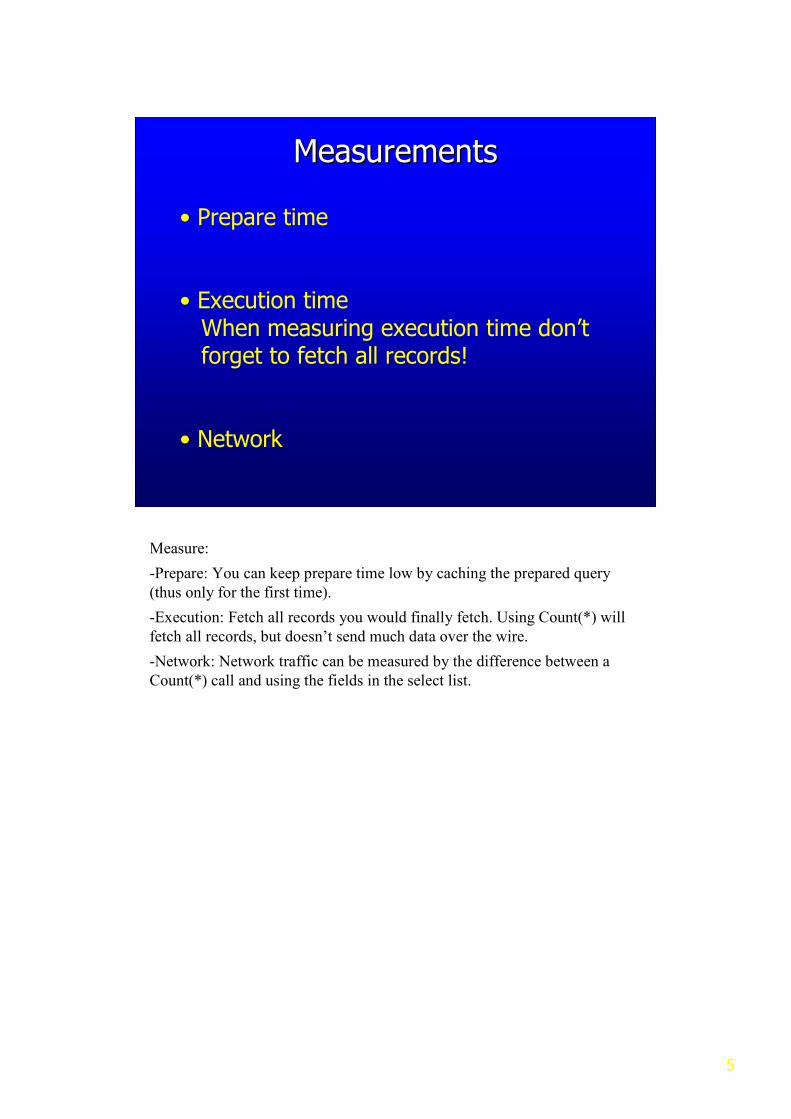
MeasurementsMeasurements
• Prepare time
• Execution timeWhen measuring execution time don’tforget to fetch all records!
• Network
Measure:
-Prepare: You can keep prepare time low by caching the prepared query
(thus only for the first time).
-Execution: Fetch all records you would finally fetch. Using Count(*) will
fetch all records, but doesn’t send much data over the wire.
-Network: Network traffic can be measured by the difference between a
Count(*) call and using the fields in the select list.

6
Performance AnalysisPerformance Analysis
• PLANread from left to right
• Reads / Writes- Non-indexed- Indexed
PLAN is the readable form of the way how internally the execution path will
be processed.
Reads and writes gives you the number of successful record-fetches/record-
updates.

7
Execution PLAN Execution PLAN
The execution PLAN explains which path/process the engine will use to
fetch/update the data. Most tools have the possibility to show you
the PLAN (for example in ISQL with SET PLAN ON).
The returned PLAN can contain the next items:
• PLAN
• NATURAL (In storage order)
• ORDER (Out of storage order)
• INDEX (indexed retrieval)
• JOIN (inner/outer join)
• MERGE (merge two streams)
• SORT
Almost every database tool can give you the PLAN from a query. Some give
you even a nice graphical screen with some hints about the PLAN.
When asking for a PLAN the optimizer converts the RSB tree into a
readable format using the keywords:
- PLAN (Start of a RSB tree)
- NATURAL (Sequential, In storage order)
- ORDER (Navigation, Out of storage order)
- INDEX (Retrieval by bitmap)
- JOIN (Inner/left/right/full join streams)
- MERGE (Merge two rivers)
- SORT (Sorting stream)
8
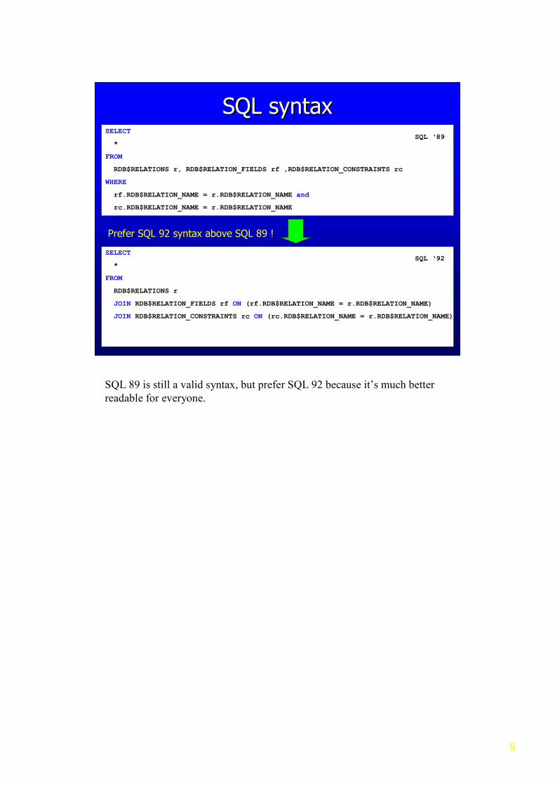
SQL syntaxSQL syntaxSELECT
*
FROM
RDB$RELATIONS r, RDB$RELATION_FIELDS rf ,RDB$RELATION_CONSTRAINTS rc
WHERE
rf.RDB$RELATION_NAME = r.RDB$RELATION_NAME and
rc.RDB$RELATION_NAME = r.RDB$RELATION_NAME
SQL ‘89
SELECT
*
FROM
RDB$RELATIONS r
JOIN RDB$RELATION_FIELDS rf ON (rf.RDB$RELATION_NAME = r.RDB$RELATION_NAME)
JOIN RDB$RELATION_CONSTRAINTS rc ON (rc.RDB$RELATION_NAME = r.RDB$RELATION_NAME)
Prefer SQL 92 syntax above SQL 89 !
SQL ‘92
SQL 89 is still a valid syntax, but prefer SQL 92 because it’s much better
readable for everyone.

9
NEVER MIX SQL 92 and SQL 89 syntax!
SQL syntaxSQL syntax
SELECT
*
FROM
RDB$RELATIONS r,
RDB$RELATION_FIELDS rf
LEFT JOIN RDB$RELATION_CONSTRAINTS rc ON(rc.RDB$RELATION_NAME = r.RDB$RELATION_NAME)
WHERE
rf.RDB$RELATION_NAME = r.RDB$RELATION_NAME

10
Join order I (ODS 10)Join order I (ODS 10)SELECT * FROM
Table_1000 t1
JOIN Table_100 t2 ON (t2.ID = t1.ID)
JOIN Table_10 t3 ON (t3.ID = t2.ID)
• T1
• T1, T2
• T1, T2, T3
• T1, T3
• T1, T3, T2
• T2
• T2, T1
• T2, T1, T3
• T2, T3
• T2, T3, T1
• T3
• T3, T1
• T3, T1, T2
• T3, T2
• T3, T2, T1
Assume that in this example all the ID’s of the tables are unique. Then the
optimizer (ODS 10) will try all the combinations you see and pick the
cheapest cost from it.

11
Join order I (ODS 11)Join order I (ODS 11)SELECT * FROM
Table_1000 t1
JOIN Table_100 t2 ON (t2.ID = t1.ID)
JOIN Table_10 t3 ON (t3.ID = t2.ID)
• T3
• T3, T2
• T3, T2, T1
• T2 • T1
When using Firebird 2.0 with ODS 11 the number of combinations is
limited to chose above.
The number of combinations starting with T2 and T1 stops already by the
first combination, because the cost is already higher.
12
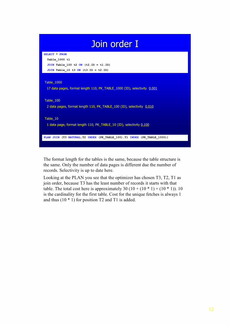
Join order IJoin order I
Table_1000
17 data pages, format length 110, PK_TABLE_1000 (ID), selectivity 0.001
Table_100
2 data pages, format length 110, PK_TABLE_100 (ID), selectivity 0.010
Table_10
1 data page, format length 110, PK_TABLE_10 (ID), selectivity 0.100
SELECT * FROM
Table_1000 t1
JOIN Table_100 t2 ON (t2.ID = t1.ID)
JOIN Table_10 t3 ON (t3.ID = t2.ID)
PLAN JOIN (T3 NATURAL,T2 INDEX (PK_TABLE_100),T1 INDEX (PK_TABLE_1000))
The format length for the tables is the same, because the table structure is
the same. Only the number of data pages is different due the number of
records. Selectivity is up to date here.
Looking at the PLAN you see that the optimizer has chosen T3, T2, T1 as
join order, because T3 has the least number of records it starts with that
table. The total cost here is approximately 30 (10 + (10 * 1) + (10 * 1)). 10
is the cardinality for the first table. Cost for the unique fetches is always 1
and thus (10 * 1) for position T2 and T1 is added.
13
Statistics (ODS 10)Statistics (ODS 10)
SELECT
i.RDB$RELATION_NAME,
i.RDB$INDEX_NAME,
i.RDB$STATISTICS
FROM
RDB$INDICES i
WHERE
i.RDB$RELATION_NAME IN ('TABLE_10', 'TABLE_100', 'TABLE_1000')
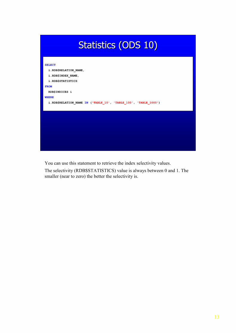
You can use this statement to retrieve the index selectivity values.
The selectivity (RDB$STATISTICS) value is always between 0 and 1. The
smaller (near to zero) the better the selectivity is.

14
Statistics (ODS 11)Statistics (ODS 11)
SELECT
i.RDB$RELATION_NAME,
i.RDB$INDEX_NAME,
i.RDB$STATISTICS,
ixs.RDB$FIELD_NAME,
ixs.RDB$STATISTICS
FROM
RDB$INDICES i
JOIN RDB$INDEX_SEGMENTS ixs ON (ixs.RDB$INDEX_NAME = i.RDB$INDEX_NAME)
WHERE
i.RDB$RELATION_NAME IN ('TABLE_10', 'TABLE_100', 'TABLE_1000')
ORDER BY
i.RDB$RELATION_NAME,
i.RDB$INDEX_NAME,
ixs.RDB$FIELD_POSITION
In ODS 11 selectivity is also stored per segment. This statement can be used
to get the segment selectivity's.
15
Join order IIJoin order II
• T1
• T1, T2
SELECT * FROM
Table_1000 t1
JOIN Table_100 t2 ON (t2.ID = t1.ID)
LEFT JOIN Table_10 t3 ON (t3.ID = t2.ID)
• T2
• T2, T1
PLAN JOIN (JOIN (T2 NATURAL,T1 INDEX (PK_TABLE_1000)),T3 INDEX (PK_TABLE_10))
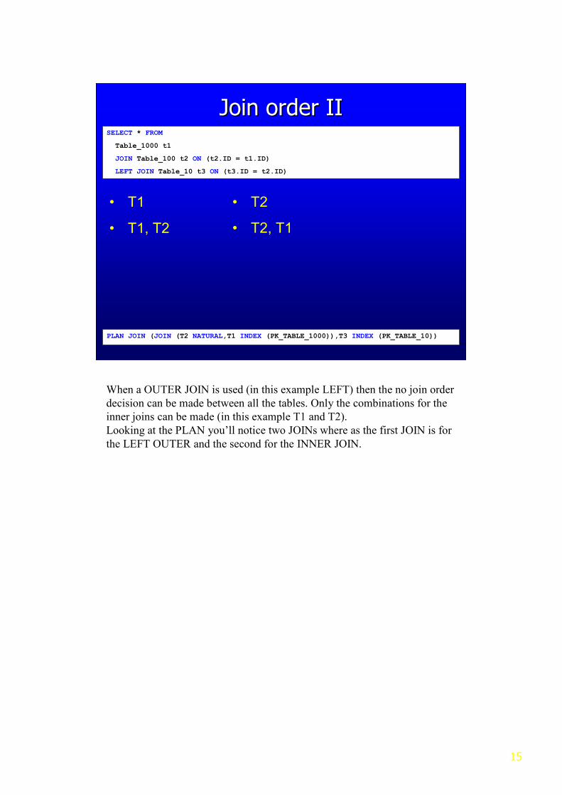
When a OUTER JOIN is used (in this example LEFT) then the no join order
decision can be made between all the tables. Only the combinations for the
inner joins can be made (in this example T1 and T2).
Looking at the PLAN you’ll notice two JOINs where as the first JOIN is for
the LEFT OUTER and the second for the INNER JOIN.

16
Join order IIIJoin order IIISELECT * FROM
Table_1000 t1
LEFT JOIN Table_100 t2 ON (t2.ID = t1.ID)
JOIN Table_10 t3 ON (t3.ID = t2.ID)
PLAN JOIN (JOIN (T1 NATURAL,T2 INDEX (PK_TABLE_100)),T3 INDEX (PK_TABLE_10))
The optimizer can not change the order.
Enter the LEFT JOINs as low as possible.
Using the OUTER in the middle as shown in this example the optimizer is
not able to make decision about the JOIN order. When you need LEFT
JOINs place them so low as possible so the optimizer can make decisions
for the JOIN order where possible.

17
Join order IV Join order IV -- VIEWVIEWCREATE VIEW VIEW1 (ID) AS
SELECT t1.ID FROM
Table_1000 t1
JOIN Table_100 t2 ON (t2.ID = t1.ID)
JOIN Table_10 t3 ON (t3.ID = t2.ID)
PLAN JOIN (T1 NATURAL,V1 T3 INDEX (PK_TABLE_10),V1 T2 INDEX (PK_TABLE_100) ,V1 T1 INDEX (PK_TABLE_1000))
SELECT * FROM
Table_10 t1
JOIN View1 v1 ON (v1.ID = t1.ID)
When possible INNER JOINs are combined to one
INNER JOIN.
In a phase before calling the optimizer multiple INNER JOINs are combined
together to 1 INNER JOIN where possible. VIEWs are flattened where
possible and combined too.
18
Join order V Join order V -- VIEWVIEWCREATE VIEW VIEW2 (ID) AS
SELECT t1.ID FROM
Table_1000 t1
JOIN Table_100 t2 ON (t2.ID = t1.ID)
LEFT JOIN Table_10 t3 ON (t3.ID = t2.ID)
PLAN JOIN(JOIN(JOIN(V1 T2 NATURAL,V1 T1 INDEX (PK_TABLE_1000),V1 T3 INDEX (PK_TABLE_10),T1 INDEX (PK_TABLE_10))
SELECT * FROM
Table_10 t1
JOIN View2 v1 ON (v1.ID = t1.ID)
Can not combine the INNER JOINs due the
LEFT JOIN at the end.
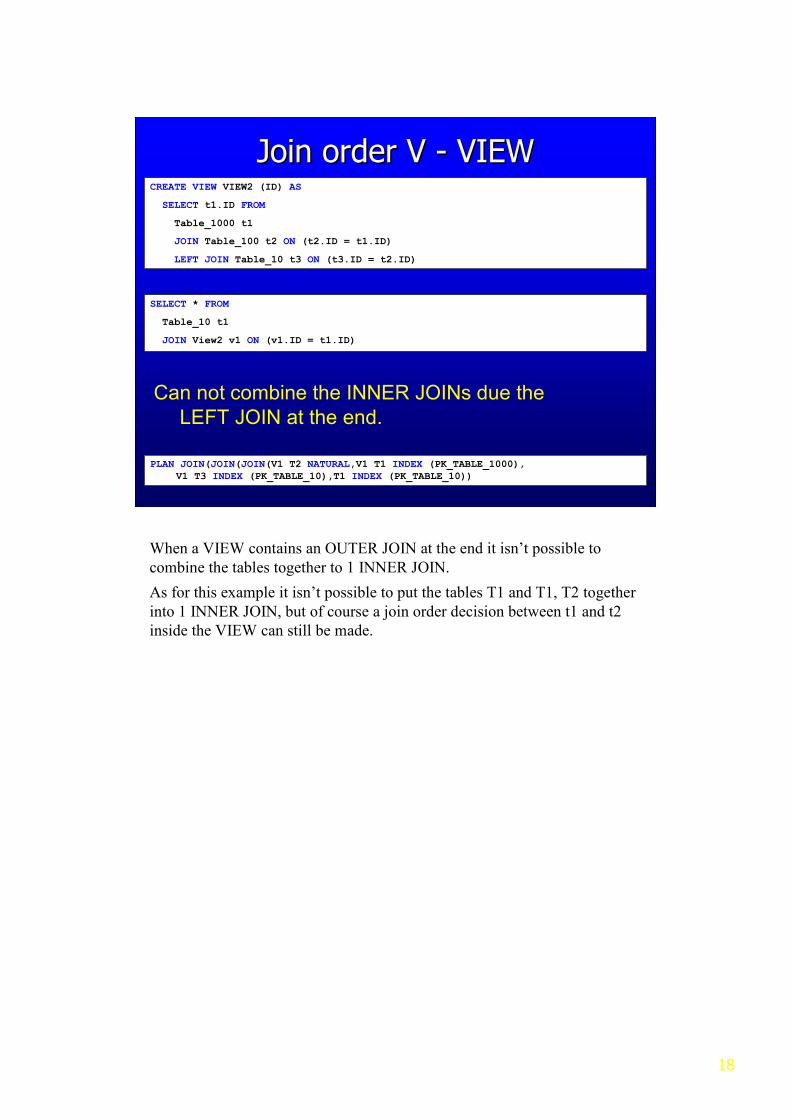
When a VIEW contains an OUTER JOIN at the end it isn’t possible to
combine the tables together to 1 INNER JOIN.
As for this example it isn’t possible to put the tables T1 and T1, T2 together
into 1 INNER JOIN, but of course a join order decision between t1 and t2
inside the VIEW can still be made.

19
Stream access IStream access ICREATE TABLE Customer (
ID INTEGER NOT NULL,
FirstName VARCHAR(50),
LastName VARCHAR(50),
CONSTRAINT PK_Customer PRIMARY KEY (ID)
)
SELECT
Count(*)
FROM
Customer c
PLAN (C NATURAL)
Running this select statement will cause Firebird to read the whole table. It
reads all records in storage order (the order it’s stored on disk) and this is the
fastest way, because when it was using an index it still has to look for every
record in the database. This is needed, because it has to check if the index
entry was valid for our current transaction.

20
Stream access IIStream access II
SELECT
c.*
FROM
Customer c
ORDER BY
c.ID
PLAN (C ORDER PK_CUSTOMER)
Using the PK in the ORDER BY here causes that the optimizer chooses for
an navigation through index. This will also read the whole table, but in the
PK order. The data isn’t stored in any specific order in the data pages, thus
this is a good candidate for random disk read.
Note that I use “c.*” in this example, but normally you wouldn’t do that.
Only put the fields you need in the select list to keep the network traffic so
small as possible.

21
Stream access IIIStream access III
SELECT
FIRST 10
c.*
FROM
Customer c
ORDER BY
c.ID
PLAN (C ORDER PK_CUSTOMER)
The index used for an ORDER is only useful when you fetch the first x records.
With FIRST x (or just fetching the first x records at the client) it’s useful
when an index is used for reading data from the disk. Now only the first 10
records are fetched from disk. Without an index on field ID the whole table
would need to be read first and sorted afterwards. Which would be more
expensive for this statement.

22
Stream access IVStream access IV
CREATE ASC INDEX IDX_CUSTOMER_LASTNAME ON Customer (LastName)
SELECT
c.LastName,
Count(*)
FROM
Customer c
GROUP BY
c.LastName
PLAN (C ORDER IDX_CUSTOMER_LASTNAME)
If the fields in the GROUP BY can be matched against an index (in the same
order) it will use this index for navigation. Note that for this example using a
SORT afterwards is faster, because all records are read. Maximum 1 index
can be used for navigation.

23
SELECT
r.LastName,
Count(*)
FROM
Relations r
GROUP BY
r.LastName
Stream access VStream access V
How to make sure the index won’t be used for navigation?
PLAN (R ORDER IDX_RELATIONS_LASTNAME)
SELECT
c.LastName,
Count(*)
FROM
Customer c
GROUP BY
c.LastName, c.LastName
PLAN SORT ((C NATURAL))
SELECT
c.LastName || '',
Count(*)
FROM
Customer c
GROUP BY
1
To avoid that an index is chosen for navigation you can add another (or the
same) field to the GROUP BY clause or “concatenate with an empty string”
/ “add a zero”. The same can be done for the ORDER BY clause.

24
Stream access VIStream access VI
SELECT
c.LastName,
Count(*)
FROM
Customer c
WHERE
c.ID = 10121
GROUP BY
c.LastName
PLAN (R ORDER IDX_RELATIONS_LASTNAME)PLAN (C ORDER IDX_CUSTOMER_LASTNAME INDEX (PK_CUSTOMER))
Is it possible to use an index for a filter, while using an index for navigational access?
Firebird 1.5 will show you only PLAN (C ORDER
IDX_CUSTOMER_LASTNAME), but internally it will use the index
available with ID in it. Firebird 2.0 will output the PLAN with ORDER and
INDEX together.

25
DSQL conversions IDSQL conversions I
SELECT * FROM
Customer c
WHERE
c.ID IN (10, 11, 12)
SELECT * FROM
Customer c
WHERE
c.ID = 10 OR
c.ID = 11 OR
c.ID = 12
The IN predicate is converted inside the DSQL (Dynamic SQL) to multiple
OR statements.
26
DSQL conversions IIDSQL conversions II
SELECT * FROM
Customer c
WHERE
c.ID IN (SELECT o.Customer_ID FROM Orders o)
SELECT * FROM
Customer c
WHERE
EXISTS(SELECT o.Customer_ID FROM Orders o
WHERE o.Customer_ID = c.ID)
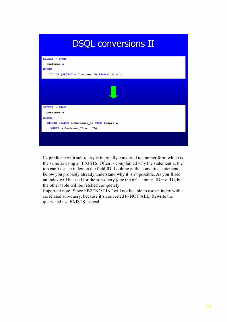
IN predicate with sub-query is internally converted to another form which is
the same as using an EXISTS. Often is complained why the statement at the
top can’t use an index on the field ID. Looking at the converted statement
below you probably already understand why it isn’t possible. As you’ll see
an index will be used for the sub-query (due the o.Customer_ID = c.ID), but
the other table will be fetched completely.
Important note! Since FB2 “NOT IN” will not be able to use an index with a
correlated sub-query, because it’s converted to NOT ALL. Rewrite the
query and use EXISTS instead.

27
DSQL conversions IIIDSQL conversions III
SELECT o.* FROM
Orders o
WHERE
o.ID IN (SELECT ch.Orders_ID FROM Customer_History ch WHERE ch.Customer_ID = 1)
SELECT o.* FROM
(SELECT DISTINCT ch.Orders_ID FROM Customer_History ch
WHERE ch.Customer_ID = 1) ch
JOIN Orders o ON (o.ID = ch.Orders_ID)
Rewrite the query
If the sub-query from an IN predicate is pretty expensive to execute and will
finally only match on a few records it could be interesting to rewrite the
query. Turn the sub-query into a derived table with DISTINCT or GROUP
BY and JOIN with the original relation (table/view/SP). The derived table
will be executed first and the relation is joined on it.

28
DSQL conversions IVDSQL conversions IV
SELECT * FROM
Customer c
WHERE
c.ID IN (SELECT Max(o.Customer_ID) FROM Orders o)
SELECT * FROM
Customer c
WHERE
EXISTS(SELECT Max(o.Customer_ID) FROM Orders o
HAVING Max(o.Customer_ID) = c.ID)
When the sub-query is an aggregate query (it has GROUP BY/HAVING or
aggregate function in the statement) the condition goes the HAVING clause
instead off the WHERE clause. This can have a big impact on performance,
because the HAVING clause is performed after the grouping.
The optimizer in Firebird 2.0 will try to distribute the condition to WHERE
clause, so an index can be used when available.

29
DSQL conversions VDSQL conversions V
SELECT * FROM
Customer c
WHERE
c.ID IN (SELECT FIRST 1 o.Customer_ID FROM Orders o)
SELECT * FROM
Customer c
WHERE
EXISTS(SELECT FIRST 1 o.Customer_ID FROM Orders o
WHERE o.Customer_ID = c.ID)
Warning, In Firebird 1.5 and before the IN predicate would probably not do
what you expect. The sub-query is evaluated for every record from the
master query and thus this will return all records for Relations.
This problem is fixed in FB2 and this sub-query is internally using a inner
joining derived table.

30
DSQL conversions VIDSQL conversions VI
SELECT * FROM
Customer c
WHERE
NOT c.ID <> 10
SELECT * FROM
Customer c
WHERE
c.ID = 10
In Firebird 2.0 NOT conditions are simplified where possible, so that the
optimizer eventually can match it against an index.

31
Operators / predicates IOperators / predicates ICan use an index:
� equals (a = b)
� less than (a < b)
� greater than (a > b)
� less than or equal (a <= b)
� greater than or equal (a >= b)
� IS NULL
� STARTING WITH
� IN with list of constants
� BETWEEN
� not equal to (a <> b)
� IS NOT NULL
� CONTAINING
� LIKE
� IN (subquery)
� NOT
Can’t use an index:

32
Operators / predicates IIOperators / predicates IIAn index can only be used inside the subquery:
� IN (subquery)
� EXISTS (subquery)
� SINGULAR (subquery)
� ALL (a # ALL (subquery))
� ANY (a # ANY (subquery))
� SOME (a # SOME (subquery))
# = (=, <, >, <=, >=, <>)
33
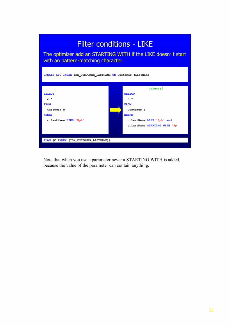
Filter conditions Filter conditions -- LIKELIKE
CREATE ASC INDEX IDX_CUSTOMER_LASTNAME ON Customer (LastName)
SELECT
c.*
FROM
Customer c
WHERE
c.LastName LIKE 'Sp%'
PLAN (C INDEX (IDX_CUSTOMER_LASTNAME))
internal
SELECT
c.*
FROM
Customer c
WHERE
c.LastName LIKE 'Sp%' and
c.LastName STARTING WITH 'Sp'
The optimizer add an STARTING WITH if the LIKE doesn’t start
with an pattern-matching character.
Note that when you use a parameter never a STARTING WITH is added,
because the value of the parameter can contain anything.

34
Filter conditions Filter conditions -- BETWEENBETWEEN
SELECT
c.*
FROM
Customer c
WHERE
c.LastName BETWEEN 'D' and 'A'
PLAN (C INDEX (IDX_CUSTOMER_LASTNAME))
internal
SELECT
c.*
FROM
Customer c
WHERE
c.LastName >= 'D' and
c.LastName <= 'A'
The optimizer converts a “between” conjunction into a “greater than or equal” and a “less than or equal” conjunction.

35
Filter conditions Filter conditions -- OROR
SELECT
c.*
FROM
Customer c
WHERE
c.ID = 11 or
c.ID = 23 or
c.ID = 44 or
c.ID = 56
PLAN (C INDEX (PK_CUSTOMER, PK_CUSTOMER, PK_CUSTOMER, PK_CUSTOMER))
With an OR filter only indexes can be used when every condition can use a
index, because if one condition can’t use an index it has to be evaluated
against every record in the table.

36
Filter conditions Filter conditions –– ANDAND
SELECT
c.*
FROM
Customer c
WHERE
c.ID => 1000 and
c.LastName < 'F'
PLAN (C INDEX (PK_CUSTOMER,IDX_CUSTOMER_LASTNAME))
If possible and it’s interesting (versus cost) two indexes will be used and
internally the indexed results are AND-ed. The final result (list of record
numbers) is used to lookup the records.

37
Filter conditions Filter conditions –– compound indexcompound index
SELECT
c.*
FROM
Customer c
WHERE
c.FirstName = 'Adam' and
c.LastName = 'Kern'
PLAN (C INDEX (IDX_CUSTOMER_FIRSTLASTNAME))
CREATE ASC INDEX IDX_CUSTOMER_FIRSTNAME ON Customer (FirstName)
CREATE ASC INDEX IDX_CUSTOMER_FIRSTLASTNAME ON Customer (FirstName, LastName)
Field order in compound index is important!
An index with two or more fields (compound index) can be very useful if
you filter a lot against the same fields with an equality operator. This index
will probably also have a good selectivity, because mostly the number if
distinct nodes will decrease. Using a field which is unique in a compound
index meant in most cases that the index is in fact unneeded/wrong.

38
Filter conditions Filter conditions –– compound indexcompound index
SELECT
c.*
FROM
Customer c
WHERE
c.FirstName > 'Adam' and
c.LastName = 'Kern'
PLAN (C INDEX (IDX_CUSTOMER_LASTNAME, IDX_CUSTOMER_FIRSTNAME))
CREATE ASC INDEX IDX_CUSTOMER_FIRSTLASTNAME ON Customer (FirstName, LastName)
When the first segments are not matched with an equal’s
operator then the next segments cannot be efficiently used.
39
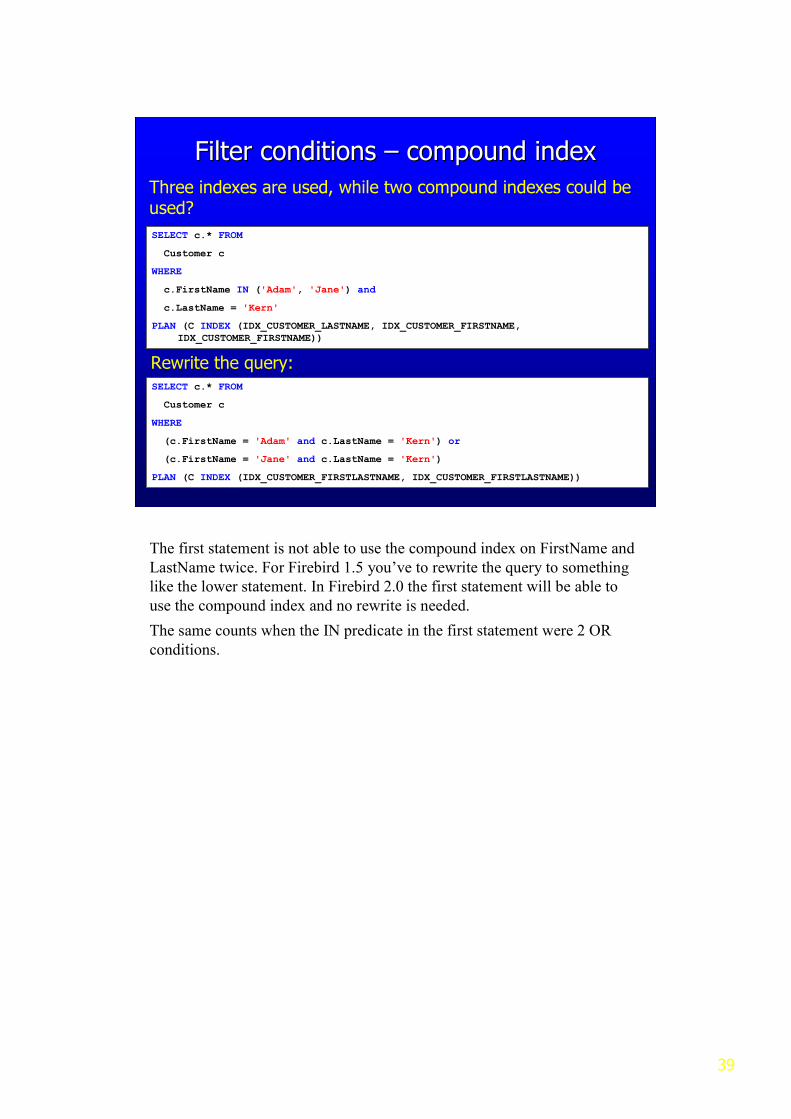
Filter conditions Filter conditions –– compound indexcompound index
SELECT c.* FROM
Customer c
WHERE
c.FirstName IN ('Adam', 'Jane') and
c.LastName = 'Kern'
PLAN (C INDEX (IDX_CUSTOMER_LASTNAME, IDX_CUSTOMER_FIRSTNAME,IDX_CUSTOMER_FIRSTNAME))
Three indexes are used, while two compound indexes could beused?
SELECT c.* FROM
Customer c
WHERE
(c.FirstName = 'Adam' and c.LastName = 'Kern') or
(c.FirstName = 'Jane' and c.LastName = 'Kern')
PLAN (C INDEX (IDX_CUSTOMER_FIRSTLASTNAME, IDX_CUSTOMER_FIRSTLASTNAME))
Rewrite the query:
The first statement is not able to use the compound index on FirstName and
LastName twice. For Firebird 1.5 you’ve to rewrite the query to something
like the lower statement. In Firebird 2.0 the first statement will be able to
use the compound index and no rewrite is needed.
The same counts when the IN predicate in the first statement were 2 OR
conditions.

40
Filter conditions Filter conditions –– ignore indexignore index
SELECT
c.*
FROM
Customer c
WHERE
c.ID + 0 > 100 and
c.LastName || '' = 'Kern'
PLAN (C NATURAL)
The optimizer can only use a index when at the left or right side from the operator 1 field is present.
SELECT
c.*
FROM
Customer c
WHERE
c.ID > 100 and
(c.LastName = 'Kern' or 1 = 0)
PLAN (C NATURAL)
Add 0 or empty string: Add OR:

41
Filter conditions Filter conditions –– LEFT JOINLEFT JOINSELECT
*
FROM
Table_1000 t1
LEFT JOIN Table_100 t2 ON (t2.ID = t1.ID)
JOIN Table_10 t3 ON (t3.ID = t1.ID)
WHERE
t2.SomeField = 'Firebird'
PLAN JOIN (JOIN (T1 NATURAL,T2 INDEX (PK_TABLE_100)),T3 INDEX (PK_TABLE_10))
Using a filter on a LEFT JOIN let the LEFT JOIN
behave as an INNER JOIN (except checking for
NULL state).
When filtering on an OUTER JOIN in the WHERE clause you let the
OUTER clause behave as an INNER JOIN. The only exception here is if
you’re checking for NULL states in the WHERE clause (such as for
“t2.SomeField IS NULL” or “COALESCE(t2.SomeField, 0) = 0”).
This is also a way to force the order in which the tables are JOINed, but it’s
recommended to let the optimizer decide. Assuming data grows and the
tables are changing in size compared to each other.

42
Filter conditions Filter conditions –– aggregateaggregate
SELECT
c.FirstName,
Count(*)
FROM
Customer c
GROUP BY
c.FirstName
HAVING
c.FirstName = 'Joe'
PLAN (C ORDER IDX_CUSTOMER_FIRSTLASTNAME)
Use the WHERE clause whenever possible.
SELECT
c.FirstName,
Count(*)
FROM
Customer c
WHERE
c.FirstName = 'Joe'
GROUP BY
c.FirstName
Filters in the HAVING clause cannot use an index. Always prefer filters in
the WHERE clause, only filters on aggregate functions should be put in the
HAVING clause.
Firebird 2.0 will try to distribute the HAVING clause to the WHERE clause
by itself.

43
Expression IndexExpression Index
SELECT
o.ID,
o.NetAmount + o.Tax
FROM
Orders o
WHERE
o.NetAmount + o.Tax BETWEEN 100 and 120
PLAN (O INDEX (IDX_ORDERS_TOTALAMOUNT))
CREATE INDEX IDX_ORDERS_TOTALAMOUNT ON Orders COMPUTED BY (NetAmount + Tax)
A new feature since FB2.0 is expression indexes. Those can be very helpful
if you’re filtering on specific expressions.
One example is for example create an expression index on a character field
with the UPPER function. This way you could search case-insensitive (of
course you need to put the search value also in UPPER) without creating a
shadow column.

44
AggregateAggregate
SELECT Max(FirstName) FROM Customer c
PLAN (C ORDER IDX_CUSTOMER_FIRSTNAME_DESC)
Max/Min Will use an index when possible.
SELECT Min(FirstName) FROM Customer c
PLAN (C ORDER IDX_CUSTOMER_FIRSTNAME_ASC)
SELECT Max(FirstName), Count(*) FROM Customer c
PLAN (C NATURAL)
When a single Min or Max aggregate function is used it will try to use an
index for navigation. Min can only use Ascending indexes and Max can
only use descending indexes.

45
SubqueriesSubqueries II
SELECT
c.LastName || ', ' || c.FirstName,
(SELECT Count(*) FROM Orders o WHERE o.Customer_ID = c.ID)
FROM
Orders o
JOIN Customer c ON (c.ID = o.Customer_ID)
ORDER BY
1
PLAN (C INDEX (PK_CATEGORIES))
PLAN SORT(JOIN(R NATURAL,RC INDEX (FK_RELCAT_RELATIONS)))
• Have their own PLAN.
• Correlated subqueries are executed for every ‘row’.

46
SubqueriesSubqueries IIII
SELECT
c.LastName || ', ' || c.FirstName,
(SELECT Count(*) FROM OrderLine ol WHERE ol.Orders_ID = o.ID)
FROM
Customer c
JOIN Orders o ON (o.Customer_ID = c.ID)
ORDER BY
2
PLAN (OL INDEX (FK_ORDERS_ID))
PLAN (OL INDEX (FK_ORDERS_ID))
PLAN SORT(JOIN(C NATURAL,O INDEX (FK_CUSTOMERID_1)))
Note! When ORDER BY or GROUP BY clause refer to a subqueryin select list then this subquery will be executed twice.

47
UNIONUNION
SELECT c.LastName || ', ' || c.FirstName
FROM Customer c
WHERE c.ID >= 1 and c.ID <= 10
UNION ALL
SELECT c.LastName || ', ' || c.FirstName
FROM Customer c
WHERE c.ID >= 101 and c.ID <= 110
ORDER BY
1
PLAN (C INDEX (PK_CUSTOMER))
PLAN (C INDEX (PK_CUSTOMER))
• Every query-item has a PLAN.
• Prefer UNION ALL above UNION.
Every query used on the left and right side of an UNION has it’s own
PLAN. When you don’t need to eliminate duplicate rows use the UNION
ALL, because this doesn’t use the distinct operation afterwards. Using just
UNION will always cause an distinct being added internally, but you can’t
read this info from the PLAN output.

48
UNION UNION -- VIEWVIEW
CREATE VIEW View3 (Orders_ID) AS
SELECT ch.Orders_ID
FROM Customer_History ch
WHERE ch.Product_ID = 16
UNION ALL
SELECT ch.Orders_ID
FROM Customer_History ch
WHERE ch.Product_ID = 24
PLAN JOIN((V CH INDEX (FK_CUSTOMER_HISTORY2))
PLAN (V CH INDEX (FK_CUSTOMER_HISTORY2)), O INDEX (PK_ORDERS))
SELECT
o.*
FROM
Orders o
JOIN View3 v ON (v.Orders_ID = o.ID)
UNION is processed first.
Unions are processed first on the same level. That’s why you see here the
view at the beginning of the PLAN.

49
UNION UNION -- distributedistribute
PLAN (V RC INDEX (FK_CUSTOMER_HISTORY2))
PLAN (V RC INDEX (FK_CUSTOMER_HISTORY2))
SELECT
v.*
FROM
View3 v
WHERE
v.Orders_ID BETWEEN 200000 and 205000
Firebird 1.5
PLAN (V CH INDEX (FK_CUSTOMER_HISTORY, FK_CUSTOMER_HISTORY2))
PLAN (V CH INDEX (FK_CUSTOMER_HISTORY, FK_CUSTOMER_HISTORY2))
Firebird 2.0
For Firebird 1.5 the filter in the WHERE clause will only be evaluated after
the whole VIEW is executed, while the relationID is also part of an index. In
Firebird 2.0 the WHERE clause on a UNION (in this case the VIEW, but it
could also be a derived table) will be distributed and other indexes could
probably be chosen. Such as in this example where the index from the
primary key could be used.
50
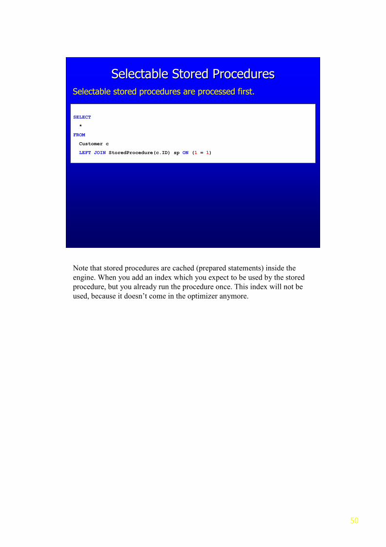
Selectable Stored ProceduresSelectable Stored Procedures
SELECT
*
FROM
Customer c
LEFT JOIN StoredProcedure(c.ID) sp ON (1 = 1)
Selectable stored procedures are processed first.
Note that stored procedures are cached (prepared statements) inside the
engine. When you add an index which you expect to be used by the stored
procedure, but you already run the procedure once. This index will not be
used, because it doesn’t come in the optimizer anymore.

51
DONDON’’T USE EXPLICIT T USE EXPLICIT PLANsPLANs!!
DONDON’’TT
USEUSE
EXPLICITEXPLICIT
PLANsPLANs!!

52
QuestionsQuestions??
53
The EndThe End