Indian Labor Regulations and the Cost of Corruption:

Evidence from the Firm Size Distribution∗

Amrit Amirapu and Michael Gechter†

November 2014

Abstract

This paper investigates the effects of an important but little-researched set of Indian

labor and industrial regulations. We use a novel methodology to provide a) the first

objective cost estimates of any Indian labor regulations and b) evidence of their impact

on misallocation of resources across firms. Our methodology takes advantage of the fact

that some regulations only apply to establishments which hire 10 or more employees.

Using data from India’s 2005 Economic Census, we observe that the distribution of

establishments by size closely follows a power law, but with a significant drop in the

distribution for establishments with 10 or more workers. Guided by a model based on

Garicano, Lelarge, and Van Reenen (2013) - but augmented to allow for the possibility

of misreporting - we use this drop to estimate the implied costs of the regulation. We

find that there is substantial variation in our estimated costs across states, industries

and ownership types, and that our costs are more robustly correlated with measures

of corruption than with any other factors, suggesting that poor state implementation

may be as much or more to blame for the high costs than the regulations themselves.

We find further that higher costs are associated with lower rates of future employment

growth in registered (but not unregistered) manufacturing, suggesting that these costs

may play a role in encouraging informality.

∗Preliminary draft. We wish to thank Dilip Mookherjee, Arvind Subramanian, Kevin Lang, HiroakiKaido, Kehinde Ajayi, Sam Bazzi and Marc Rysman for their input, guidance and encouragement. Wealso thank Laveesh Bhandari, Aditya Bhattacharjea, Sharon Buteau, Areendam Chanda, Urmila Chatterjee,Nancy Chau, Bivas Chaudhuri, Bibek Debroy, Francois Gourio, Jayinthi Harinath, Rana Hasan, Ravi Kan-bur, Saibal Kar, Dan Keniston, Devashish Mitra, Sandip Mitra, G. Sajeevan, Johannes Schmieder, PronabSen, Anushree Sinha, Sandip Sukhtankar, Shyam Sundar, John Van Reenen and conference and seminar par-ticipants at NEUDC, BU, University of Passau, Cornell, ISI Kolkata and IGIDR for many useful comments.Representatives in the state governments of BR, KL, MH, TN and WB provided invaluable assistance inunderstanding the data collection process for the Economic Census. We gratefully acknowledge financial sup-port from the Weiss Family Program Fund for Research in Development Economics. Liu Li, Stefan Winataand Haiqing Zhao provided expert research assistance, supported by the BU MA-RA mentor program.†Boston University; aamirapu@bu.edu, mgechter@bu.edu

1 Introduction

India’s labor and industrial regulations have been blamed for many of the country’s ills,

including low levels of aggregate productivity, slow growth of productivity, and lackluster job

creation in the formal sector1 (e.g. Hsieh and Klenow (2009); Kochhar, Kumar, Rajan, and

Subramanian (2006); Besley and Burgess (2004); Hasan and Jandoc (2012)). Of particular

note is Hsieh and Klenow (2009)’s landmark study, in which the authors argue that aggregate

total factor productivity in India could be 40%-60% higher if not for significant misallocation

of resources across firms. They go on to suggest that India’s labor regulations may be to

blame for the observed misallocation, although they leave the job of fully corroborating

this link to others. In fact, the view that labor regulations are of primary importance is

not universally held. Many argue that the laws as written are rarely enforced so that, in

practice, firms are effectively unconstrained.2 Others argue that the existing evidence on the

detrimental impact of labor regulations is flawed (Bhattacharjea (2006, 2009)). Still others

point out that the vast majority of regulations have gone unstudied while nearly all of the

attention from economists and the press has focused on a single regulation (Chapter VB of

the Industrial Disputes Act) - one that is not likely to constrain any but the very largest

firms (Bardhan (2014)).3

It is the goal of this paper to address the above aspects of this debate while avoiding

some of the criticisms that have been leveled at previous work. In particular, we use a novel

methodology and a uniquely well-suited dataset to study the behavior of firms in response

to regulatory thresholds in order to determine whether and to what extent firms are in

fact constrained by regulations.4 We proceed in the following steps. First, we generate the

establishment-size distribution using data from the Economic Census of India (EC), which,

importantly, aims to be a complete enumeration of all non-farm business units, regardless

of size or status (formal or informal). From the distribution, we observe that it closely

follows a power law, except for a discontinous and proportional decrease in the density of

establishments with 10 or more workers. This is precisely the threshold at which a multitude

of regulations become legally binding, so we take this observation as evidence that firms with

1Here and elsewhere in the paper, the formal sector refers to business enterprises that are registered withsome branch of the government.

2For instance, in a recent paper, Chaurey (2015) provides evidence that firms seem to hire contractworkers as a way of avoiding certain regulations.

3Chapter VB of the Industrial Disputes Act (IDA) stipulates that firms in the industrial sector with 100or more workers must obtain permission from the relevant governmental authority before laying off workers.Bardhan (2014) points out that 92 percent of firms in the garmet sector have less than 8 workers.

4Note: for expositional purposes we occasionally refer to “firms”, although it would be more correctto refer to “factories” or “establishments”, since all of the data and most of the regulations are at thefactory/establishment level rather than the firm level. Regardless, the disinction is almost moot: nearly allIndian firms are single factory/establishment firms.

2

10 or more workers do seem to be constrained in size by certain regulations - although these

are not the same regulations that most others have focused on. We then develop a model

of firm size choice under regulatory thresholds which is based on Garicano et al. (2013)

(henceforth GLV), but augmented to explicitly allow for the possibiliy of misreporting.5 We

model the regulations as causing an increase in the unit labor costs of those firms that report

having exceeded the 10 worker threshold6, and then use the observed distortion in the size

distribution to estimate these costs. Under our primary estimation method at the All-India

level, we find that firms behave as if operating at or above the 10-worker threshold entailed

a 35% increase in their per-worker costs.

Our next step is to document substantial heterogeneity in the size of our estimated costs

along several dimensions including state, industry and ownership type. For example, we

find that the state with the highest estimated regulatory costs is Bihar and that privately-

owned establishments have the highest costs, while government-owned establishments have

the lowest. Exploring this variation further, we find that our estimated costs turn out to be

correlated with some previous state-level measures of labor regulation reforms (in particular,

certain measures from Dougherty (2009)), though not with others (for example, the Besley-

Burgess measure from Aghion, Burgess, Redding, and Zilibotti (2008)).7 Moreover, we find

strong and robust correlations between our estimated costs and two quite distinct measures

of corruption8, even after controlling for a number of factors including state GDP per capita.

As further support for our state-level results, we show that industries with greater “regulatory

dependence” have higher estimated costs, but only when they are located in more corrupt

states.9 We take these correlations to be suggestive of the fact that the true cost of the

regulations may have more to do with bureacracy and corruption, rather than the content

of labor and industrial regulations themselves.

Finally, we turn to a brief discussion of the possible dynamic consequences of the costs we

estimate. We show that, while higher costs are associated with slower growth in employment

and productivity in the registered manufacturing sector, this association is more muted

5Misreporting was a lesser concern in GLV’s original setting, as they had access to administrative data.In contrast, the data in the Economic Census are self-reported, which makes the threat of deliberate misre-porting more significant in our case.

6This is the only way to generate a proportional decrease in the theoretical density, at least in a staticmodel.

7This may reflect the fact that the Besley-Burgess measures focus on the IDA, while the regulations westudy are entirely different. On the other hand, if the Besley-Burgess measures are meant to capture thegeneral effect of labor laws at the state level, one might expect the two measures to be correlated.

8These corruption measures include a subjective, perceptions-based measured of corruption from Trans-parency International and a measure of the percentage of electricity that is lost in transmission and distribu-tion as reported by the Reserve Bank of India (this latter measure has been used as a proxy for governmentcorruption and ineffectiveness in, for example, Kochhar et al, 2006).

9We measure “regulatory dependence” by taking the industry average of the number of inspector visitsamong Indian firms in the 2005 World Bank Enterprise Surveys.

3

- or even in the opposite direction - in the unregistered manufacturing sector, where the

regulations are less salient. This suggests that the costs we estimate may play a role in the

“informalization” of the Indian economy, by pushing workers from the formal to the informal

sector.

This paper aims to contribute to at least three important strands of literature. The first,

which we have already mentioned, is the literature on misallocation of resources and total

factor productivity (TFP), as exemplified by Hsieh and Klenow (2009). Our contribution is

to provide direct evidence that at least some of the misallocation of resources across firms

in India is tied to regulations or the enforcement thereof.10 In particular, we show that size-

based regulations (or at least the ways in which they are enforced) lead firms to fall short of

their optimal scale, thus distorting the allocation of labor among firms in the economy and,

likely, lowering TFP.

Another strand of literature to which we aim to contribute relates to corruption in the

enforcement of government policies. Most previous studies (eg: Besley and McLaren (1993);

Mookherjee and Png (1995)) have modeled such corruption as collusion between inspectors

and firms or citizens: corrupt inspectors allow firms to avoid the de jure costs of abiding

by regulations in exchange for bribes. Hence, in these frameworks, corruption lowers the

costs associated with regulations. However, our results suggest that the costs associated

with size-based regulations are higher in more corrupt environments, and are thus more in

line with an alternative framework in which corruption takes the form of extortion between

inspectors and firms (i.e.: corrupt inspectors take advantage of bureacratic regulations in

order to extract higher rents from firms in the form of harassment bribes).11 We present

a theoretical model as well as anecdotal evidence from “ipaidabribe.com” to support this

interpretation and view the support we provide for this alternative conception of corruption

to be another contribution of the paper.

Lastly, this paper is also clearly related to the large literature that more generally inves-

tigates the impact of Indian labor regulations on economic outcomes. The literature dates

back to at least Fallon and Lucas (1993), but the more recent proliferation seems to be due to

the work of Besley and Burgess (2004). In that paper, the authors first interpret state-level

amendments to the Industrial Disputes Act (IDA) as either “pro-worker” or “pro-employer”

and then aim to show that Indian states that amended the IDA in a “pro-worker” direction

experienced slower growth in output, employment, investment and productivity in registered

manufacturing. The paper, though extremely influential, has been criticized by Bhattachar-

10In future work we hope to determine what portion of the TFP loss from misallocation estimated byHsieh and Klenow (2009) can be attributed to the regulations we study.

11This finding echoes Novosad and Asher (2012), in which it is argued that regulations can provide ameans through which politicians can impose costs on businesses.

4

jea (2006) and Bhattacharjea (2009) on a number of grounds. One of Bhattacharjea’s major

criticisms is that Besley and Burgess’s interpretations of amendments as “pro” or “anti-

worker” are subjective and debatable (ie: different people might read and code them in a

different way). This criticism affects most of the subsequent academic work on this topic,

since most papers use the Besley-Burgess codings, but it is a criticism we are able to sidestep

with our methodology. Since our analysis is based only on firm level data and size-thresholds

stated explicitly in the laws themselves, it has the advantage of objectivity.

The second contribution we make to this literature is to focus on a set of regulations

that have been almost entirely ignored even though they effect a much larger proportion

of firms than Chapter VB of the IDA.12 The only other papers of which we are aware that

study regulations that kick in at the 10-worker threshold are Dougherty (2009), Dougherty,

Frisancho, and Krishna (2014) and Kanbur and Chatterjee (2013). The latter investigates the

Factories Act, which applies to all manufacturing firms that use power and have 10 or more

workers (or don’t use power and have 20 or more workers), but their focus is to document non-

compliance under the act, which we see as complementary to our approach of estimating the

costs of the regulations.13 The papers by Dougherty and co-authors employ state-level indices

of labor reforms that differ from the Besley-Burgess codes in that they include consideration

of non-IDA regulations such as the Factories Act, but they are constructed from surveys

of industry experts and, as such, are by and large subject to similar concerns regarding

subjectivity.

Another way in which we distinguish ourselves from the previous literature on Indian

regulations is that we explore the effect of regulations in all non-farm segments of the In-

dian economy - not just in registered manufacturing, on which nearly all previous academic

studies have focused. A final contribution of the paper is to provide suggestive evidence that

improper government enforcement of regulations may play a role in shifting employment

from the registered to the unregistered sector.

In the next section (Section 2), we provide an overview of the relevant institutional details

regarding Indian labor and industrial regulations. Section 3 introduces the data and covers

some basics about the size distribution of enterprises in India. In Section 4 we go over the

theoretical model and our corresponding empirical strategy. Section 5 provides the main

results. In Section 6, we interpret the findings, explore the multiple dimensions of variation

12Chapter VB of the IDA only applies to manufacturing firms with 100 or more workers. In contrast, theregulations we study affect all firms with 10 or more workers and are thus relevant for a much larger share offirms. We have also tried analyzing Chapter VB of the IDA using the same methodology we employ for theregulations with the 10 worker threshold, but find no effects. I.e.: there does not seem to be a proportionaldecrease in the density of establishments with more than 100 workers. We also fail to observe “bunching”of firms at sizes just below 100, although the presence of rounding may make such bunching impossible todiscern even if it exists.

13Our estimated costs are robust to the possibility of noncompliance.

5

in our results, and investigate the connection between our estimated costed and corruption.

Section 7 concludes.

2 Institutional Background: Size-Based Regulations in

India

In this paper we attempt to investigate the effects of certain size-based industrial and labor

regulations in India. These are regulations that only apply to establishments that exceed

a certain size, measured either in terms of a firm’s revenue, the amount of fixed capital

invested, or the number of workers employed. One of the most significant such thresholds

occurs when establishments employ 10 or more workers, after which they must register with

the government and meet various workplace safety requirements (under the Factories Act14,

for example), pay social security taxes (under the Employees’ State Insurance Act), distribute

gratuities (under the Payment of Gratuity Act) and bear a greater administrative burden

(under, e.g., the Labor Laws Act).

Not only are the laws numerous, it has been argued that certain components of the

laws are antiquated and/or arbitrary. For example we read in the “India Labour Report”

that “Rules under the Factories Act, framed in 194815, provide for white washing of factories.

Distemper won’t do. Earthen pots filled with water are required. Water coolers won’t suffice.

Red-painted buckets filled with sand are required. Fire extinguishers won’t do... And so on”

TeamLease Services (2006). Firm owners who choose not to comply with such regulations

may face costs if discovered and convicted.16

In addition to - or in lieu of - the explicit costs of complying with the regulations,

establishments with 10 or more workers may be subject to implicit costs associated with

increased interaction with labor inspectors, et al, who may have the power to extract bribes

and tighten (or ease) the administrative burden firms face. Indeed, inspectors in India have

a large amount of discretion regarding the enforcement of administrative law. For example,

in some cases, the definition of what constitutes a “day” is at the discretion of the inspector,

and it is a commonly held view that “[w]hile grave violations are ignored, minor errors

become a scope for harassment” (TeamLease Services (2006)).

This kind of behaviour has been referred to as “harassment bribery” (Basu (2011)).

Anecdotal evidence of inspectors using the complexity and sheer amount of paperwork as

14Technically the Factories Act applies for 10-plus worker establishments only if they use power. Forestablishments that do not use power, the Factories Act does not apply until they employ 20 workers.

15The Factories Act itself dates to 1948, but the origins of the law go back another 100 years at least, toBritain’s first Factory Acts.

16These costs may include fines and/or prison sentences.

6

a way to extract bribes is easy to come by. For example, we have included a selection of

citizen reports from “ipaidabribe.com” in Appendix 2, which demonstrate just this kind of

behaviour.17 Interestingly, some of the reports suggest that the size of the bribe paid is a

direct linear function of the number of employees - which will be relevant to our estimation

procedure later.

As we alluded to earlier, the 10 worker threshold is not the only one relevant; there are

other cutoffs at which different regulations become binding. For example, the threshold that

seems to have received the most attention, both from academics and the press, is that of 100

workers, at which enterprises in most states become subject to Chapter VB of the Industrial

Disputes Act, under which they must be granted government permission to lay off workers.

There are other cutoffs still,18 but in this paper we will focus on estimating some of the costs

and effects associated with the regulations that come into force at the 10 worker cutoff. One

important limitation of our analysis is that we will not be able to address issues regarding

the efficacy of any regulations in promoting worker welfare.

3 Data and the Size Distribution in India

3.1 Data

The data we rely on to investigate the 10-worker threshold comes from the Economic Census

(EC) of India. The EC is meant to be a complete enumeration of all (formal and informal)

non-farm business establishments19 in India at a given time, regardless of their size. It is this

last clause that makes the EC different from every other data source available and precisely

suited to our needs. Although the 2005 dataset contains a large number of observations

(almost 42 million), there is not very detailed information collected on each observation.

For each establishment in the data, there is only information on a handful of variables

including the total number of workers usually working, the number of non-hired workers

(such as family members working alongside the owner), the registration status, the 4-digit

NIC industry code, the type of ownership (private, government, etc) and the source of funds

17We thank Andrew Foster for this suggestion.18For example, firms with 20 or more workers must abide by the Provident Funds Act. Firms with 50 or

more workers must comply with Chapter VA of the Industrial Disputes Act, which requires them to providecompensation and notice to employees prior to lay-offs.

19The EC refers to these as “entreprenuerial units” and defines them as any unit “engaged in the productionor distribution of goods or services other than for the sole purpose of own consumption.” As is common inthe literature, we occasionally refer to them as “firms” even though the unit of observation in the data isactually a factory or an establishment, rather than a firm (i.e.: multiple establishments may belong to thesame firm). We do this for expositional purposes and justify our use of this convention with the observationthat the proportion of establishments that belong to multi-establishment firms is minute.

7

for the establishment. There is no information on capital, output or profits, and the data is

cross-sectional.

The EC has rarely been used in academic papers - possibly because it is cross-sectional,

contains a significant amount of measurement error, and only contains information on the

handful of variables just enumerated, so that better data sources exist for most purposes.

The EC is ideal for our purpose, however, since it includes information on employment size

and covers the entire universe of establishments. Other more commonly used datasets, such

as the CMIE’s Prowess Database, the Annual Survey of Industries (ASI) or the National

Sample Survey’s (NSS) Unorganized Manufacturing Surveys cover only certain parts of the

distribution and thus cannot be used for our purpose. The ASI, for example, only covers

factories in the manufacturing sector that have registered with the government under the

Factories Act. However, registration under this Act is only required for establishments with

10 or more workers if the unit uses power (20 or more workers if the factory uses no power).

Therefore, the selection of the ASI varies discontinuously at precisely the point of interest.

Similar limitations on coverage make the other datasets - other than the EC - unsuitable.

Aside from the Economic Census, we also supplement our analysis with data from a

variety of other sources. From the ASI we get employment and productivity in the registered

manufacturing sector. We generate those same variables for the unregistered sector with

data from the Ministry of Statistics and Programme Implementation (MOSPI) and the

Reserve Bank of India (RBI). We get data on state and industry level corruption from a)

Transparency International’s “India Corruption Study 2005”, b) the RBI, and c) the World

Bank Enterprise Survey for India (2005). Data on State-level regulatory enforcement come

from the Indian Labour Year Book.20 Other measures of state-level regulations come from

Aghion et al. (2008) and Dougherty (2009), while industry-level measures of exposure to

trade liberalization come from Ahsan and Mitra (2014).

3.2 The Size Distribution of Establishments in India

Figure 1 below shows the distribution of establishments by the number of total workers (hired

and non-hired workers) for establishments with up to 200 total workers in 2005. Perhaps

the most striking feature of figure 1 is the extraordinary degree to which the distribution

is right-skewed. Indeed, about half of all establishments are single person enterprises, while

the densities for establishments with 10 or more workers are almost imperceptible.21 Figure

2 shows the drop in density for establishments with 10 or more workers in detail and figure

20We would like to thank Anushree Sinha and Avantika Prabhakar for their considerable and generoushelp in obtaining these data.

21The densities for establishments with more than 200 workers are also imperceptible. We have omittedthem only for clarity in the figure.

8

Figure 1: Distribution of establishment size for establishments with 1-200 total workers, 2005

3 shows the full distribution of establishment size frequencies according to a log scale. Each

point represents one bar in the earlier histograms.

Two things are most striking about figure 3. First, the natural log of the density is a

linear function of the natural log of the number of total workers. This implies that the

unlogged distribution follows an inverse power law in the number of total workers. This

pattern will be important for the analysis that follows but it is not very surprising in and

of itself: power law distributions in firm sizes have been documented in many countries (e.g.

Axtell (2001) and Hernandez-Perez, Angulo-Brown, and Tun (2006)). The second and more

unique feature of the distribution is that there appears to be a level shift downward in the log

frequency for establishment sizes greater than or equal to 10. Figure 4 shows this effect for

establishments with fewer than 100 workers by running an OLS regression of the log density

against log firm size and allowing the intercept to vary for firms with 10 or more workers.

To the best of our knowledge, ours is the first paper to document this phenomenon in India.

Also of note from the figures above is that there appears to be a significant amount of non-

classical measurement error, seemingly due to rounding of establishment sizes to multiples

of 5 and 10. The existence of rounding is not surprising given that the data are self-reported

and that respondents are asked to give the “number of persons usually working [over the

last year]”. Partially to alleviate concerns that the non-classical measurement error due to

rounding might bias our results (and partially for other reasons to be made explicit shortly),

we will employ an estimation procedure which first smooths the data non-parametrically.

9

Figure 2: Distribution of establishment size for establishments with 5-25 total workers, 2005

Figure 3: Distribution of establishment size, 2005, log scale

Figure 4: Downward shift at the 10-worker threshold in the distribution of establishmentsize, 2005, log scale (omitting establishments with more than 100 workers)

10

4 Model and Empirical Strategy

4.1 Basic Model

To interpret the downward shift from Figure 4 in economic terms, we turn to the model in

GLV. In their framework, size-based regulations are assumed to increase the unit labor costs

of firms that exceed the size threshold, which results in a downshift in part of the theoretical

firm size distribution. From the magnitude of the downshift they observe in the empirical

distribution they attempt to estimate the additional labor costs imposed by the regulations.

GLV begin with a distribution of managerial ability (α ∼ φ(α)) as the primitive object,

following Lucas (1978). As is common in the literature (e.g. Eaton, 2011), they assume

that the distribution of managerial ability follows a power law (e.g. φ(α) = cαα−βα). It

is this that will generate a power law in the theoretical firm size distribution. A firm with

productivity or managerial ability α faces the following profit-maximization problem:

π(α) = maxn

αf(n)− wτn

where n is the number of workers a firm employs, f(n) is a production function (with

f ′(n) > 0 and f ′′(n) < 0), w is a constant wage paid to all workers, and τ is a proportional

tax on labor that takes the value 1 if n ≤ N and τ if n > N , where τ > 1.

From the first order condition on this maximization problem, α = wτf ′ (n)

, one can see that

higher productivity establishments/managers will employ more workers, and that firms which

cross the threshold (N) and must therefore pay higher labor costs will hire fewer workers

than they would otherwise. This latter feature is built to match the observed “downshift”

in the actual firm size distribution to the right of the regulatory threshold.

One can informally characterize the solution as follows: one set of managers with partic-

ularly low productivity (below some threshold α1) will be effectively unconstrained. These

managers would have chosen to hire fewer than 10 workers whether or not the regulation was

present. Another set of managers with slightly higher productivity (between some thresh-

olds α1 and α2) would, in the absence of the regulation, have chosen to hire 10 or more

workers - but who, in the presence of the regulation, obtain higher profits by hiring only 9

workers to avoid the discontinuous increase in costs implied by crossing the threshold. These

mangers should be “bunched up” at 9. The last set of managers are those with high enough

productivity (α > α2) that it is not worth it to avoid the regulation and so they choose to

exceed the threshold and pay the tax. However, these managers face higher marginal costs

than they would in the absence of the regulation and therefore employ fewer workers by a

constant proportion (resulting in a “downshift” in the logged firm size distribution).

An exact expression for the distribution of firm size, χ(n), can be recovered as a trans-

11

formation of the distribution of managerial ability, φ(α), since the first-order conditions on

the firms’ maximization problems imply a monotonic relationship between α and n. The key

result is that a function of the tax enters multiplicatively in the expression for the density

of firms size n (for all n > 9). Therefore, the function of the tax enters additively in the log

density for all firms large enough to be subject to the tax.

Formally, the density of firms with n total workers, χ(n) is given by:

χ(n) =

(1−θθ

)1−β(β − 1)n−β if n ∈ [nmin, N)(

1−θθ

)1−β(N1−β − τ−

β−11−θ n1−β

u ) if n = N

0 if n ∈ (N, nu)(1−θθ

)1−β(β − 1)τ−

β−11−θ n−β if n ≥ nu

where θ measures the degree of diminishing returns to scale, capturing both features of

the production function and market power, β represents the negative slope of the power law

and τ is the implicit per worker tax. Taking logs and combining the first and last cases22

leads to:

log(χ(n)) = log

[(1− θθ

)1−β

(β − 1)

]− β log(n) + log(τ−

β−11−θ )1{n > 9}

This leads to an estimating equation:

log(χ(n)) = α− β log(n) + δ1{n > 9} (1)

We can identify τ according to:

τ = exp(δ)−1−θβ−1

τ is thus a function of θ, β and δ. We get estimates for α, β and δ from equation 1. Knowing

α and β pins down θ, which allows us to identify τ .

4.2 Concerns Regarding Misreporting

Before proceeding further, we must consider how our results might be affected by the pos-

sibility of misreporting. This is important because one of the underlying assumptions of

the analysis above is that the size distribution of firms as observed in the Economic Census

is accurate. However, since the data are self-reported, it is possible that plant managers

may misreport information to Economic Census enumerators. Specifically, if the managers

are aware of the increased regulatory burden that is associated with employing 10 or more

22In other words, we ignore the bunching at N and the valley directly after, since these are features thatare not easily observable in the data. Instead we focus on the ranges n ∈ [nmin, N) and n > nu.

12

workers, and if they believe that the EC enumerators will relay information to government

regulatory bodies, they may wish to hide the fact that their actual employment exceeds the

threshold. To see how this type of behavior might affect our results, we model it explicitly

in the following subsection.

A further reason to be concerned about the possibility of misreporting is due to the

fact that Economic Census enumerators were required to fill out an extra form containing

the address of any establishment that reported 10 or more workers. It is conceivable that

enumerators might have found it preferable to under-report the number of workers for es-

tablishments with 10 or more workers in order to avoid the extra burden of filling in the

“Address Slip”. Although we do not model this type of problem explicitly in what follows,

the implications are nearly identical to those of the model we do explicitly analyze.23

4.3 A Theoretical Model of Misreporting

Our model of misreporting starts with the theoretical model from Section 4.1, and amends

it to allow firms to choose not only their true employment (n), but also their reported

employment (l). Then, a firm with productivity α faces the following profit-maximization

problem:

π(α) = maxn,l

αf(n)− wn− τ l ∗ 1(l > 9)− F (n, l) ∗ p(n, l)

where α, f(n), w and τ are all defined as they were previously. The problem is identical

except that now firms pay the extra marginal cost, τ , only on their reported employment,

and not on their true employment. Furthermore, they only pay this cost if their reported

employment exceeds the threshold.24 There is now an incentive for firms to misreport their

employment in a downward direction (i.e.: to set l < n). Counteracting this incentive is

that misreporting firms may be caught by the authorities with probability p(n, l), and made

subject to a fine, F (n, l). As written above, both the probability of being caught and the

magnitude of the fine may in general depend on n and l in an arbitrary way. However, if

one is willing to make the assumption that the expected cost of misreporting (F ∗ p) is an

increasing and convex function of the degree of misreporting, n− l, it will be possible to use

an estimation technique that will be only minimally biased by the presence of misreporting.

Fortunately, based on our understanding of the context in which firms make these decisions,25

23The only difference is that higher fixed costs would replace higher marginal costs. It is, moreover, easyto show that if our estimation strategy is robust to the model of misreporting we do analyze, it is also robustto this second type of misreporting as well.

24In point of fact it is most likely that firms’ answers to Economic Census enumerators have no impact ontheir regulatory burden, but it is possible that firms believe otherwise, and that is what is relevant.

25This understanding is informed by informal interviews with small businesses in Chennai and our reading

13

we believe that this is the most reasonable assumption on the functional form of the expected

cost that one could make.

One plausible way to obtain convex misreporting costs is to suppose that firms are caught

with a probability that is linearly increasing in the degree of their misreporting (i.e.: n− l)and subject to a fine if caught which is also a linear function of their misreporting. Another

possibility is that the probability of being caught is itself an increasing and convex function

of the degree of misreporting and the fine if caught is fixed. In what follows we will assume

the latter for clarity of exposition, but the analysis is identical for any assumption that yields

convex costs of misreporting.

Specifically, suppose that misreporting firms are caught with probability p(n, l) = (n−l)2100

,

and pay a fixed fine, F , if caught. Then their profit maximization problem is:

π(α) = maxn,l

αf(n)− wn− τ l ∗ 1(l > 9)− F ∗ (n− l)2

100

The solution to this problem can be informally characterized as follows. The lowest

productivity firms (those with α below some threshold, α1) will be unconstrained, choosing

n ≤ 9 and reporting truthfully (l = n). Higher productivity firms, with α ∈ [α1, α2], will

choose n > 9, exceeding the regulatory threshold, but will find it profitable to misreport

their employment, setting l = 9. These firms will only appear to be “bunched” up at 9,

but will in fact have higher employment. The last category of firms are those with α > α2,

which are productive enough to warrant hiring work forces so large that they cannot avoid

detection with reasonable probability and must report l > 9. Even these firms, however,

with both n > 9 and l > 9 do not find it profit-maximizing to report truthfully. They

can save on their unit labor costs by shading their reported employment, and will choose

l = n − 50Fτ . Note that the degree of misreporting is by a constant amount, rather than a

constant proportion.26

More formally, the log of the density of firms with true employment n, logχ(n), is given

by:

logχ(n) =

logA− βlog(n) if n ∈ [nmin, 9)

log[ξ(n)] if n ∈ [9, nm(α2)]

0 if n ∈ (nm(α2), nt(α2))

logA′(τ)− βlog(n) if n ≥ nt(α2)

while the log of the density of firms with reported employment l, logψ(l) is given by:

of the secondary literature.26This outcome is a result of the convex cost assumption.

14

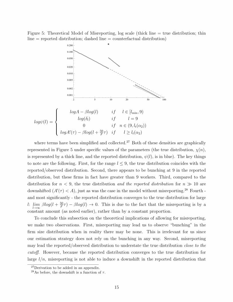
Figure 5: Theoretical Model of Misreporting, log scale (thick line = true distribution; thinline = reported distribution; dashed line = counterfactual distribution)

2 5 10 20 50 100

0.001

0.002

0.005

0.010

0.020

0.050

0.100

0.200

logψ(l) =

logA− βlog(l) if l ∈ [lmin, 9)

log(δl) if l = 9

0 if n ∈ (9, lt(α2))

logA′(τ)− βlog(l + 50Fτ) if l ≥ lt(α2)

where terms have been simplified and collected.27 Both of these densities are graphically

represented in Figure 5 under specific values of the parameters (the true distribution, χ(n),

is represented by a thick line, and the reported distribution, ψ(l), is in blue). The key things

to note are the following. First, for the range l ≤ 9, the true distribution coincides with the

reported/observed distribution. Second, there appears to be bunching at 9 in the reported

distribution, but these firms in fact have greater than 9 workers. Third, compared to the

distribution for n < 9, the true distribution and the reported distribution for n � 10 are

downshifted (A′(τ) < A), just as was the case in the model without misreporting.28 Fourth -

and most significantly - the reported distribution converges to the true distribution for large

l: liml→∞

βlog(l + 50Fτ) − βlog(l) → 0. This is due to the fact that the misreporting is by a

constant amount (as noted earlier), rather than by a constant proportion.

To conclude this subsection on the theoretical implications of allowing for misreporting,

we make two observations. First, misreporting may lead us to observe “bunching” in the

firm size distribution when in reality there may be none. This is irrelevant for us since

our estimation strategy does not rely on the bunching in any way. Second, misreporting

may lead the reported/observed distribution to understate the true distribution close to the

cutoff. However, because the reported distribution converges to the true distribution for

large l/n, misreporting is not able to induce a downshift in the reported distribution that

27Derivation to be added in an appendix.28As before, the downshift is a function of τ .

15

differs from the downshift in the true distribution at large values of l. Therefore, if we use

an estimation strategy that focuses mostly on values far from the cutoff, our estimate of

the downshift using the observed distribution is likely to reflect the real downshift and thus

we are likely to avoid this source of bias. We develop such an estimation strategy in the

following subsection.

Before proceeding, however, we should note again that the above analysis assumes that

the expected costs of misreporting are strictly convex. There exist non-convex functional

forms of the cost function which may lead one to observe a downshift in the reported distri-

bution that is greater than the one in the true distribution, thus biasing any estimates of τ

upwards.

4.4 An Empirical Strategy Robust to the Possibility of Misreport-

ing

Since convex misreporting costs imply that misreporting will only distort the distribution

of reported establishment size versus the true distribution of establishment size close to the

cutoff, we estimate the model on the full distribution of establishment size. Since estimating

equation 1 treats each establishment size as one observation, using the full distribution of

establishment size will mean that the model is primarily estimated using data far from the

10-worker cutoff.29 However, estimating equation 1 on the full distribution of establishment

size introduces two complications. First, we cannot perform the estimation on the empirical

PMF for large firm sizes, since the empirical probability mass is truncated at the reciprocal

of the number of observations (see figure 6 below), while the underlying density continues to

diminish in establishment size. Second, respondents appear to round their reported number

of workers to the nearest multiple of 5 (see figure 2), a phenomenon that is more pronounced

for larger establishments and that could bias our results.

To address these two problems, we first estimate the density associated with each number

of workers χ(n) non-parametrically using the method of Markovitch and Krieger (2000),

which addresses the econometric issues arising in nonparametric density estimation of heavy-

tailed data. We then use the nonparametric density estimates as a basis for fitting the model

in equation 1, augmented by dummy variables for having 1, 2, 8, 9 and 10 - 20 workers.30

29The largest establishment in the 2005 EC has 22,901 workers.30The rationale for flexibly modeling the density at 1 and 2 workers is that own account enterprises and 2-

worker enterprises are likely to be household enterprises and may therefore differ fundamentally in characterfrom their larger counterparts. The rationale for flexibly modeling the density at 8 and 9 workers is thatthe theory above predicts that the reported density just below the cutoff will be biased upwards by anymisreporting effects. Similarly, the theory also predicts that values above - but close to - the threshold mayalso be biased (downwards). Therefore we also flexibly control for such values (10 to 20) as well, althoughdoing so has only a very small effect on the estimates: as explained above, the estimates are driven mostly

16

Figure 6: Downward shift at the 10-worker threshold in the distribution of establishment sizeestimated on nonparametric density estimates, 2005, log scale (including all establishments).Black points = actual data; Grey = smoothed data.

Figure 6 depicts the strategy. The black dots show the raw data. The grey dots represent the

result of the first step: nonparametric density estimates associated with each establishment

size. The line shows the fit of the model in equation 1, augmented by the dummy variables,

to the nonparametric density estimates.

Figure 6 above provides some evidence for the model described in section 4.3. The

observed establishment size distribution appears to converge back to a power law with the

same slope as for establishments with fewer than 10 workers, but deviates slightly from that

slope at sizes just above the 10-worker cutoff. In the next section we report the results of

the estimation.

5 Preliminary Results

In this section we apply the estimation procedure described above to the 2005 Economic

Census of India and report the results. Standard errors obtained from a wild cluster boot-

strap procedure with 200 replications are given in parentheses.31 In the tables below, we first

report estimates for τ − 1 at the All-India level and for a selection of States, Industries and

Ownership Types. Estimates for all States, Industries and Ownership Types are reported

in the Appendix. The All-India estimate on τ − 1 is .35 and is statistically significant. This

by observations relatively far from the threshold.31We cluster at the firm size level to allow for the possibility that reporting errors may be correlated by

firm size.

17

means that, on average, establishments in India that hire more than 9 workers act as though

they must pay additional labor costs of 35% of the wage per additional worker. In the ta-

bles and figures it can be seen that there is substantial variation in the magnitude of our

estimates of the per-worker tax by State, Industry and Ownership Type. For example, the

point estimate on τ − 1 for the State of Kerala is .14, while the estimate for Bihar, on the

other hand, is .70, implying that establishments in Bihar act as though they must pay a tax

of 70% of the wage for each additional worker they hire past 9 workers.

We also observe substantial differences in the size of τ by industry: it appears that the

effective tax is highest for establishments in construction and retail. As one might expect,

the tax is nonexistent for establishments in the public administration sector (in fact it is

negative, but this seems to result from the fact that the assumed power law does not fit the

distribution of establishments in this sector well). Similarly, when looking at the differences

by ownership type, we find that the estimates for τ are highest for private firms (especially

unincorporated proprietorships), and nonexistent (or negative) for government-owned firms,

where presumably the regulatory burden is less than in the private sector.

Estimates of τ by State Using the Full Distribution of Establishment Size

Level τ − 1

All-India

.347

(0.059)

By State

Bihar .693

(0.069)

Gujarat 0.165

(0.047)

Kerala 0.138

(0.033)

Uttar Pradesh 0.502

(0.069)

By Industry

Construction .478

(0.047)

18

Manufacturing .268

(0.039)

Wholesale, retail .637

(0.115)

Public admin., social security -.311

(0.031)

By Ownership Type

Government and PSU -.092

(0.028)

Unincorporated Proprietary .490

(0.005)

6 Discussion and Investigation of Mechanisms

6.1 Interpretation of Results

Thus far we have argued that the observed downshift in the distribution of establishments

with 10 or more workers is related to the existence of certain labor and industrial regulations

that become binding at that point. But if the regulations are responsible for the observed

effect, then differences in the substance or application of the regulations should explain (at

least part of) the great variation we observe across States and Industries.32 In this section

we explore these dimensions of variation with the goal of reaching a deeper understanding

regarding the causes and consequences of the costs we have tried to estimate. The regressions

we do are cross-sectional and the variables used are endogenous, so the results cannot be

given a causal interpretation, but we find them instructive nevertheless.

To preview our results, we do observe a correlation between our estimated costs (τ)

and certain measures of the substance of the regulations. Moreover, we also find a robust

and independent correlation between our estimated costs and several different measures of

32The variation across ownership types is straightforward to explain: the regulations are clearly not appliedin the same way to privately owned enterprises and government enterprises. An additional explanation isthat government establishments are not profit maximizing and thus would require a different motivationaltheory altogether to produce the observed power law distribution.

19

corruption/poor state governance, suggesting that it is not only the regulations themselves

but also their enforcement and application that is responsible for the high costs we estimate.

We also sketch a theoretical framework of bribery and extortion which casts light on the

proper interpretation of our empirical results. Finally, we present some suggestive evidence

that our costs may have significant negative dynamic implications, as they are associated

with lower growth in employment and productivity in registered manufacturing - and higher

growth in employment in unregistered manufacturing.

6.2 τ and Corruption: Evidence from the Interstate Variation

We start by regressing our state-level estimates of τ against other established measures of the

regulatory environment (see Table 2).33 These measures include the “Besley Burgess” (BB)

measure of labor regulations from Aghion et al. (2008) and several measures from Dougherty

(2009). The first is a measure of the number of amendments that a state government has

made to the Industrial Disputes Act in either a “pro-worker” or “pro-employer” direction, as

interpreted by Aghion et al. (2008), who update the measure to include amendments up to

1997.34 Positive values indicate more “pro-worker” amendments, which are assumed to imply

a more restrictive environment for firms operating in those states. Dougherty (2009) also

provides state level measures that reflect “the extent to which procedural or administrative

changes have reduced transaction costs in relation to labor issues” Dougherty et al. (2014).

Higher values therefore indicate an improved environment for firms. Dougherty’s measures

are unique in that they cover a wide range of labor-related issues - not just the IDA. In

the analysis below, we will focus on measures from Dougherty (2009) that cover reforms

regarding 1) the Factories Act and 2) an overall measure of reforms. All relevant variables

in our analysis have been rescaled to have mean zero and standard deviation one, with the

goal of allowing comparability between regression coefficients in different specifications.

In Table 2, correlations are reported between τ and the three measures both by themselves

and while controlling for other factors (notably state GDP per capita and the state’s share

of employment in manufacturing). The Besley Burgess (BB) measure does not seem to be

correlated with τ (although our power is limited by the very small number of observations)

while the two measures from Dougherty (2009) are significantly correlated after applying

controls (though not all the correlations are strongly significant) and have the “correct”

sign: states that saw more “transaction cost reducing” reforms have lower τs. 35 On the one

33Note that the estimates of τ we use in all the analysis below were generated using the procedure inSection 4.4 that we have argued is robust to possible misreporting and non-classical measurement error.

34Since there have been few state-level amendments to the IDA between 1997 and 2005, this measureshould be largely the same in 2005.

35In this and most of the analysis ahead, we focus on the 18 largest Indian States, for which data are most

20

hand the lack of correlation between τ and the BB measure is not surprising, as the latter

capture variation only due to state amendments to the Industrial Disputes Act, which does

not vary over the ten person threshold. On the other hand, if the Besley Burgess measure

is meant to capture the general regulatory environment (which is how it is used in countless

studies), we might well expect it to correlate with our measure of regulatory costs. That the

correlation does not hold may therefore be of interest.

While the prediction regarding the correlation between τ and BB 97 may be ambiguous,

that is not the case for Dougherty’s measures of transaction-cost reducing reforms related

to the Factories Act. We should expect our measure of τ to correlate negatively with the

latter, since the Factories Act does vary across the 10 worker threshold, and indeed we see

that it does. τ is also correlated with Dougherty’s more comprehensive measure of reforms,

one which aggregates reforms across all areas, although it does not appear to correlate with

any other subcomponents (which are not depicted here).

Table 2: Tau vs Other Measures of Regulations(1) (2) (3) (4) (5) (6) (7) (8) (9)tau tau tau tau tau tau tau tau tau

Besley-Burgess -0.0734 -0.00841 0.0481measure (regs) (0.204) (0.192) (0.172)

Dougherty measure -0.289 -0.407∗∗ -0.408∗

(all reforms) (0.201) (0.174) (0.198)

Dougherty measure -0.211 -0.318∗ -0.304(FA reforms) (0.187) (0.166) (0.181)

log of net state -0.432∗ -0.592∗∗ -0.604∗∗ -0.575∗∗ -0.590∗∗ -0.605∗∗

domestic product pc (0.226) (0.214) (0.206) (0.241) (0.217) (0.257)

share of employment -3.490 2.657 3.899 2.962 3.486 4.215in manufacturing (4.886) (5.090) (3.281) (4.934) (3.435) (5.163)

share of privately -11.66 2.003 0.529owned establishments (6.768) (5.895) (6.221)

share of registered 3.042∗ -0.0440 0.654establishments (1.530) (1.476) (1.469)

Constant 0.641∗∗∗ 5.315∗∗ 15.79∗∗ 0.653∗∗∗ 6.207∗∗∗ 4.259 0.631∗∗∗ 6.091∗∗ 5.481(0.204) (2.165) (6.707) (0.187) (1.962) (6.113) (0.189) (2.068) (6.517)

Observations 15 15 15 18 18 18 18 18 18

* p¡0.10, ** p¡0.05, *** p¡0.01, Standard errors in parentheses

Only including Major Indian States

In addition to the above measures regarding state-level changes to the statutory, proce-

consistently available and which offer the most precise estimates of τ (the power law relationship breaksdown in smaller states when there are not enough observations).

21

dural and administrative aspects of the regulations, we also regress τ against certain other

measures of the labor environment. Table 3 reports the results of τ regressed against per

capita measures of strikes, man-days lost to strikes, lockouts and man-days lost to lockouts.

One might imagine that strikes and lockouts capture relevant features of the regulatory and

labor environment,36 but we do not find them to be robustly correlated with τ .

One might also expect τ to be correlated with aspects of the regulatory enforcement.

To test this hypothesis we regress τ against state level variables related to enforcement

such as the number of inspections, convictions, and fines levied under various regulations.37

The results of the regressions for a subset of the enforcement related variables are shown

in Table 4. In short, the only enforcement variable that is even close to being significantly

correlated with τ is the percentage of factories registered under the Factories Act that have

been inspected. However, as can be seen from the table, the enforcement data are only

available for a small subset of the major states, leaving very little power in the regressions.

Furthermore, the regressions shown exclude Uttar Pradesh, which is a substantial outlier in

the enforcement data.

36For example, some industrial regulations explicitly undermine or support the rights of parties to engagein strikes or lockouts.

37These data were obtained from the 2005 Indian Labour Yearbook, which we were able to attain withthe generous help of Anushree Sinha and Avantika Prabhakar of NCAER.

22

Table 3: Tau vs Strikes and Lockouts(1) (2) (3) (4) (5) (6) (7) (8)tau tau tau tau tau tau tau tau

strikes per capita -0.272∗ -0.196(0.145) (0.148)

mandays lost due to -0.119 -0.148strikes per capita (0.157) (0.159)

lockouts per capita -0.0544 -0.0915(0.146) (0.143)

mandays lost due to -0.0527 -0.0995lockouts per capita (0.145) (0.139)

log of net state -0.400 -0.493∗ -0.506∗∗ -0.515∗∗

domestic product pc (0.234) (0.238) (0.235) (0.235)

share of employment 2.548 4.482 3.831 3.754in manufacturing (3.644) (4.171) (3.995) (3.913)

Constant 0.721∗∗∗ 4.352∗ 0.646∗∗∗ 5.017∗∗ 0.620∗∗∗ 5.191∗∗ 0.618∗∗∗ 5.291∗∗

(0.187) (2.204) (0.212) (2.272) (0.198) (2.221) (0.197) (2.222)Observations 18 18 17 17 18 18 18 18

Standard errors in parentheses

Only including Major Indian States∗ p < 0.10, ∗∗ p < 0.05, ∗∗∗ p < 0.01

23

Table 4: Tau vs Enforcement of Regulations(1) (2) (3) (4) (5) (6) (7) (8)tau tau tau tau tau tau tau tau

percent of factories 0.448∗

inspected (0.230)

convictions under FA -0.0914per factory (0.411)

prosecutions under -0.122SEA per capita (0.357)

fines under SEA per 0.323capita (0.342)

prosecutions per -0.134inspection (0.254)

fines per inspection 2.598under SEA (3.557)

cases disposed per -9.616inspection under SEA (16.45)

cases disposed per 1.058cases prosecuted under SEA (1.094)

log of net state -0.0180 -0.648 -1.545∗∗ -2.220∗∗ -1.572∗∗ -1.977∗∗ -1.471∗∗ -1.610∗∗

domestic product pc (0.921) (1.265) (0.606) (0.783) (0.537) (0.677) (0.600) (0.500)

share of employment -2.361 4.091 4.873 5.550 4.525 7.130 4.486 2.514in manufacturing (7.120) (12.61) (4.855) (4.542) (4.883) (5.277) (4.848) (5.340)

Constant 0.970 6.706 15.42∗∗ 22.20∗∗ 15.72∗∗ 20.08∗∗ 12.60 16.57∗∗∗

(8.791) (11.88) (5.835) (7.767) (5.150) (6.986) (8.218) (4.802)Observations 10 9 13 13 13 13 13 13

Standard errors in parentheses

Only including Major Indian States (except UP) for which data exist.∗ p < 0.10, ∗∗ p < 0.05, ∗∗∗ p < 0.01

To briefly summarize the results so far, when regressing τ against regulatory substance,

enforcement or industrial disputes, one only observes correlations for certain specific types

of measures of those phenomena. In contrast, in our remaining analysis, we will demon-

strate that our measures of τ are strongly and robustly correlated with corruption, almost

regardless of how it is measured. Table 5 reports the results of regressing τ against corrup-

tion as measured in a 2005 Transparency International (TI) Survey.38 Column 1 includes

all states for which there is data, while the remaining columns include only the 18 largest

Indian states. Column 3 adds controls for state GDP per capita, share of manufacturing

38The TI corruption measure is based on a survey of perceptions and experience regarding corruption inthe public sector.

24

in employment and some others, while Column 4 adds the aggregate measure of regulatory

reform from Dougherty (2009). With no exceptions, the coefficient on the TI corruption

score is consistently significant and very large in magnitude: a one standard deviation in-

crease in a state’s corruption score is associated with a .5 standard deviation increase in τ .

In particular, the fact that the coefficient remains significant in Column 4 even after control-

ling for Dougherty’s measure of regulatory reforms suggests that the relationship between

τ and corruption is at least partly independent from the relationship with the regulations

themselves.

In what follows we will use the TI corruption score as our primary measure of corruption.

One might be concerned, however, that the TI measure may be flawed as it is the result

of individuals’ perceptions (it has been argued by some that the perception of corruption

is an unreliable indicator for actual corruption). Therefore, we also regress τ against an

alternative measure of corruption that is not perception based to check for robustness of the

relationship between τ and corruption: Table 6 reports the results of τ regressed against

the percent of a state’s available electricity that was lost in transmission and distribution in

2005. This variable has been used by other researchers as a proxy for corruption and poor

state governance, and has the virtue of being a concrete and objective measure that does

not depend on perceptions Kochhar, Kumar, Rajan, Subramanian, and Tokatlidis (2006).

As with the TI Corruption Score, the correlations between τ and this alternative measure of

corruption are significant and large in magnitude regardless of sample or controls - including,

again, the addition of the Dougherty measure of regulatory reform in Column 4. To make

sure that the results are not driven by the actual transmission of electricity, we control for

per capita electricity available in Column 5 - which does not affect the results.

25

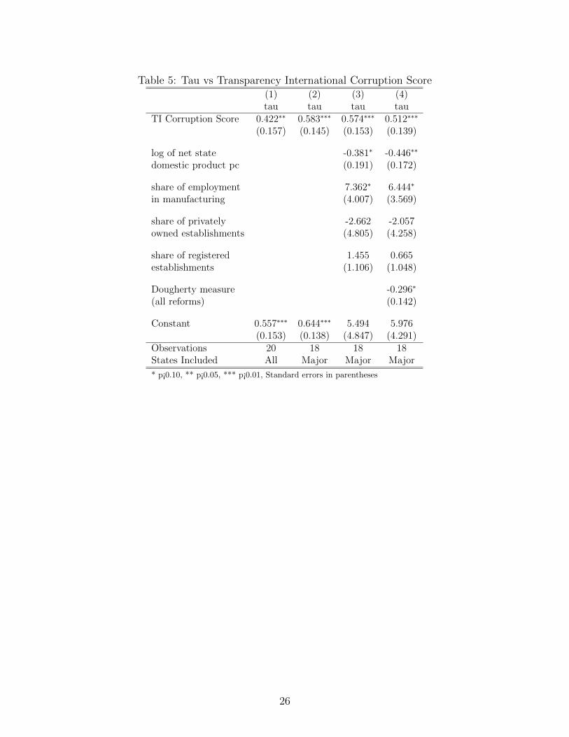
Table 5: Tau vs Transparency International Corruption Score(1) (2) (3) (4)tau tau tau tau

TI Corruption Score 0.422∗∗ 0.583∗∗∗ 0.574∗∗∗ 0.512∗∗∗

(0.157) (0.145) (0.153) (0.139)

log of net state -0.381∗ -0.446∗∗

domestic product pc (0.191) (0.172)

share of employment 7.362∗ 6.444∗

in manufacturing (4.007) (3.569)

share of privately -2.662 -2.057owned establishments (4.805) (4.258)

share of registered 1.455 0.665establishments (1.106) (1.048)

Dougherty measure -0.296∗

(all reforms) (0.142)

Constant 0.557∗∗∗ 0.644∗∗∗ 5.494 5.976(0.153) (0.138) (4.847) (4.291)

Observations 20 18 18 18States Included All Major Major Major

* p¡0.10, ** p¡0.05, *** p¡0.01, Standard errors in parentheses

26

Table 6: Tau vs Transmission and Distribution Losses(1) (2) (3) (4) (5)tau tau tau tau tau

electricity 0.318∗ 0.648∗∗ 0.663∗∗ 0.566∗∗ 0.708∗∗

transmission and distribution losses (0.165) (0.244) (0.253) (0.237) (0.268)

log of net state -0.477∗ -0.536∗∗ -0.459∗

domestic product pc (0.222) (0.205) (0.229)

share of employment 7.651 6.515 6.817in manufacturing (4.812) (4.439) (5.094)

share of privately -2.148 -1.440 -1.980owned establishments (5.677) (5.200) (5.824)

share of registered 1.513 0.644 1.577establishments (1.307) (1.284) (1.343)

Dougherty measure -0.317∗

(all reforms) (0.172)

Electricity 0.119available (GWH) (0.182)

Constant -8.42e-09 0.643∗∗∗ 5.936 6.322 5.610(0.163) (0.163) (5.746) (5.253) (5.910)

Observations 35 18 18 18 18States Included All Major Major Major Major

* p¡0.10, ** p¡0.05, *** p¡0.01, Standard errors in parentheses

Although the state-level correlations between τ and corruption appear to be robust, the

regressions lack exogenous variation and are subject to the concern that our measures of

corruption may be correlated with omitted variables that are also correlated with τ . To

partially address these concerns, we attempt to take advantage of State X Industry level

heterogeneity. In particular, inspired by Novosad and Asher (2012), we use 2005 World

Bank Enterprise Survey (WBES) data to create an industry-level measure of “dependence on

government bureaucracy”. Specifically, Indian firms in the 2005 WBES were asked how many

times in a year they had an inspection or other required meeting with a government official.

Averaging the firm-level responses by industry, we classify industries according to their

average number of visits with officials (i.e., their dependence on government bureaucracy).

If some industries have more meetings with officials, and if corruption takes place during

some of these meetings, we would imagine that the costs of corruption would be highest for

firms in those industries with the highest dependence on bureaucracy and in those states

27

that have the highest levels of corruption. That is, we would expect that the interaction

between industry level dependence on bureaucracy and state level corruption is positive. If

found to be the case, it would be harder to argue that the result is due to the presence of

omitted variables.

The hypothesis is tested in Table 7. To do so we generate our measures of τ at the

State X Industry level39 and interact each of our state level measures of corruption with a)

the industry average number of visits from officials and b) the industry average duration of

visits from officials. We include the interaction with average duration of visits as a placebo

test: it is not clear that the duration of an inspection should be positively or negatively

correlated with corruption.40 We then regress our State X Industry measures of τ against

the covariates including interaction terms. Our prior is that the interaction of corruption

with duration of visits should be less significant than the interaction with number of visits.

Indeed, this is mostly what we observe. The interaction between our measures of corruption

and the number of visits is at least weakly significant (at the 10% level) for one of the two

measures, while the interaction between corruption and average duration of visits is never

significant.

To summarize our results from these investigations, we find:

1. a correlation between τ and certain aspects of the substance of regulations as measured

in Dougherty (2009),

2. a nonexistent or inconclusive relationship between τ and measures of the labor envi-

ronment and enforcement of regulations, and

3. a strong and robust relationship between τ and two distinct measures of corruption.

Although none of these results can be said to be causal, we find them suggestive of a relation-

ship between corruption and high labor costs. Next, we turn our attention to the question

of how and why greater corruption would lead to higher labor costs for firms. To this end, in

the following subsection we outline a simple theoretical framework to elucidate the potential

connection.

39Industries here are categorized according to their groupings in the World Bank Enterprise Surveys,which distinguishes 24 distinct industry categories. Examples include “auto components”, “leather andleather products”, and “food processing”.

40In particular, corruption may lead to longer inspections if the process of extracting the bribe takes time,or it may lead to shorter inspections if corruption obviates the need to carry out the actual inspection.

28

Table 7: Tau vs State Level Corruption Interacted with Industry Level “Dependence onRegulation” (with Industry FEs)

(1) (2) (3) (4)tau tau tau tau

2005 TI 0.132∗ 0.140∗

Corruption Score (0.0668) (0.0666)

electricity 0.0583 0.0493transmission and distribution losses (0.114) (0.110)

number of 0.127 0.130inspections (0.0829) (0.0945)

duration of -0.00610 -0.109inspections (0.124) (0.143)

corruption score 0.101∗

X num inspections (0.0545)

corruption score 0.0513X duration of inspections (0.0691)

electricity TDLs 0.0112X num of inspections (0.0848)

electricity TDLs -0.0698X duration of inspections (0.107)

log of Net State -0.185∗∗∗ -0.185∗∗∗ -0.197∗∗∗ -0.194∗∗∗

Domestic Product pc (0.0364) (0.0374) (0.0428) (0.0427)

Constant -0.244 0.0235 -0.235 -0.217(0.187) (0.442) (0.187) (0.498)

Observations 189 189 189 189

* p¡0.10, ** p¡0.05, *** p¡0.01, Standard errors clustered at the State Level, Industry FEs included.

6.2.1 A Theoretical Framework for Understanding Corruption Between Inspec-

tors and Firms

We find it helpful to distinguish between two types of corruption that could take place

between inspectors and firms: collusion and extortion. Collusion takes place when inspectors

allow firms to avoid the costs of complying with regulations in exchange for bribes. However,

poor state governance (which here would imply an inability to control corruption) would then

lead to lower costs for firms, as greater corruption would make it easier to avoid the full costs

29

of regulation.41 However, what we observed in Section 6.2 was a robust positive correlation

between effective costs (τ) and poor governance/corruption. To explain this phenomenon,

we need a model of extortion. In this section, we will sketch the intuition for such a model.

A fuller (but still simple) model of extortion and bribery is provided in Appendix 3.

Let us start with the observation that all firms reporting at least 10 employees fall under

the jurisdiction of certain regulations. Imagine, now, that the regulations are so complex so

as to make it impossible (or prohibitively costly) for any firm to be fully in compliance with

all aspects of the law as written.42 Then, an inspector can, at any time, choose to subject

a firm under his jurisdiction to a penalty e, which may include financial (e.g.: fines) and/or

non-financial elements (e.g.: harassment, time needed to defend claims of violations, etc).

We can think of the extent of the penalty (e) as a function of state governance: properly

functioning governments hire and motivate inspectors to pursue substantive violations rather

than minor ones, while inspectors in corrupt or dysfunctional governments can get away with

threatening to impose high penalties for even minor technical violations if a bribe is not paid

(i.e.: extortion).

In such an environment, firms reporting 10 or more employees (and hence under the

jurisdiction of the inspector) may face a choice between exposing themselves to the penalty,

e, or paying a bribe, b. Assume that inspectors face no costs or benefits from imposing the

penalty on the firm, but naturally benefit from receiving the bribe. There is thus a surplus to

be had from paying/receiving the bribe b and avoiding the penalty. If the inspector and firm

Nash Bargain over the surplus with bargaining weights α and β, respectively, the problem

is the following:

maxb

(b)α(e− b)β

The solution is for the firm to pay a bribe b = αα+β∗ e. The cost born by the firm is

therefore increasing in α, the bargaining weight of the inspector, and in e, the maximum

penalty to which the firm can be subjected. It is reasonable to imagine that this maximum

level of extortion, e, is roughly proportional to the size of the firm, so that e = e′ ∗ n, where

n is the number of workers in the firm and e′ is the per worker level of extortion. In that

case the bribe per worker, bn, is equal to α

α+β∗ e′.43

41See, for example, a model of corruption such as the one in Khan, Khwaja, and Olken (2014).42This does not not require much imagination. As we mentioned in Section 2, many of the laws have

components that are antiquated, arbitrary, contradictory and confusing. That the laws may be impossibleto fully comply with is suggested by some of the anecdotes we provide in Appendix 2 as well as the followingobservation, which we re-quote: “Rules under the Factories Act, framed in 1948, provide for white washingof factories. Distemper won’t do. Earthen pots filled with water are required. Water coolers won’t suffice.Red-painted buckets filled with sand are required. Fire extinguishers won’t do... And so on” (TeamLeaseServices, 2006).

43Again, we provide some support for the claim that bribes are proportional to the number of workers

30

This framework can be embedded into the firm’s choice of true and reported employment

as modeled in Section 4.3. In particular, the firm now faces a choice between reporting

employment greater than or less than 10, where reporting less than 10 allows it to avoid

the costs of bribery, and reporting greater than 10 exposes it to the bribery costs. In that

framework, τ corresponds to bn, and is therefore increasing in the bargaining power of the

inspector (α) and the corruption level of the state (e′). In this way, we can make sense of

the empirical results above in terms of this basic framework. Again, a more fully fleshed

out model that explicitly incorporates features missing here (such as an appeals process and

inspector types) is provided in Appendix 3.

6.3 Possible Consequences of τ

In the subsections above, we tried to argue that our estimated costs (τ) are most likely

due, not only to the substance of the regulations themselves, but also to high levels of

corruption. In this subsection we will indicate possible consequences of high values of τ .

Again, the results cannot be given a causal interpretation, but we find them compelling

nevertheless. In what follows we use two distinct measures of τ : one which is created using

all the enterprises in a state, regardless of economic sector (τ) and another which is created

using only the enterprises engaged in manufacturing (τmanuf ).

Table 8 displays the results of employment growth in the manufacturing sector between

2010 and 2005 at the State Level regressed against our two measures of labor market dis-

tortions (τ and τmanuf ) as well competing measures (BB and Dougherty). For each of the

four measures, we observe its performance as a predictor of future employment growth in

registered manufacturing as well as its correlation with employment growth in unregistered

manufacturing. Interestingly, in the regressions of employment growth in registered manu-

facturing against τ and τmanuf , the coefficient on τ is negative and at least weakly significant,

while the coefficient for employment growth in unregistered manufacturing is positive - sig-

nificantly so in the case of τmanuf . This result makes sense: we should expect higher costs to

negatively effect the sectors to which the costs apply - in this case the registered sector, since

that is under the ambit of labor regulations while the unregistered sector is not. If these

correlations reflect a causal chain, it would mean that high levels of regulator costs and cor-

ruption (as measured by τ) are pushing employment from the registered to the unregistered

sector.

Also included in Table 8 are the results of employment growth in manufacturing re-

gressed against the BB and Dougherty measures. Neither regressor has a coefficient that

with anecdotal evidence from ipaidabribe.com in Appendix 2.

31

is statistically significant or of a meaningful magnitude.44 Putting aside the considerable

caveat that none of these results has the virtue of exogenous variation, it would appear to be

the case that our measures of labor market distortions do a better job of predicting future

employment growth (or the lack thereof) than the established alternatives. This is also true

when considering future growth in manufacturing productivity rather than employment, as

shown in Table 9. Higher levels of τ are associated with slower growth of productivity in the

registered manufacturing sector (less so in the unregistered sector)

Table 8: Manufacturing Employment Growth (2005 - 2010) vs Tau and Other Measures(1) (2) (3) (4) (5) (6) (7) (8)

reg manuf unreg manuf reg manuf unreg manuf reg manuf unreg manuf reg manuf unreg manuftau -0.0240 0.00197

(0.0176) (0.0233)

tau (manuf) -0.0471∗∗ 0.0623∗∗

(0.0217) (0.0256)

Besley-Burgess -0.00525 0.00979measure (regs) (0.00731) (0.0142)

Dougherty measure 0.0226 -0.0143(all reforms) (0.0130) (0.0159)

log of net state 0.00312 0.0189 0.0107 0.0192 0.00413 0.0140 0.0212 0.0136domestic product pc (0.0178) (0.0214) (0.0145) (0.0161) (0.00863) (0.0168) (0.0154) (0.0195)

share of employment -0.393 0.00558 -0.708∗∗ 0.435 0.0194 -0.559 -0.515∗ 0.0525in manufacturing (0.258) (0.329) (0.258) (0.325) (0.186) (0.362) (0.245) (0.323)

Constant 0.0969 -0.182 0.0372 -0.229 0.0209 -0.0675 -0.0861 -0.131(0.173) (0.209) (0.139) (0.152) (0.0825) (0.160) (0.147) (0.182)

Observations 18 17 18 17 15 15 18 17

* p¡0.10, ** p¡0.05, *** p¡0.01, Standard errors in parentheses, Only including Major Indian States

44One might argue that it is not quite fair to regress growth between 2010 and 2005 on a regressor thatuses data only up until 1997 (as is the case for the BB measure). However, a) we have duplicated theseresults using from growth from 1997 to 2002 and the results are the same, and b) the Besley Burgess measurefrom Aghion et al. (2008) should be largely the same in 2005 due to the lack of state level reforms between1997 and 2005.

32

Table 9: Manufacturing Productivity Growth (2005 - 2010) vs Tau and Other Measures(1) (2) (3) (4) (5) (6) (7) (8)

reg manuf unreg manuf reg manuf unreg manuf reg manuf unreg manuf reg manuf unreg manuftau -0.0321∗∗ 0.00522

(0.0146) (0.0239)

tau (manuf) -0.0512∗∗ -0.0567∗

(0.0181) (0.0275)

Besley-Burgess -0.00266 -0.00372measure (regs) (0.0122) (0.0154)

Dougherty measure 0.0167 0.00973(all reforms) (0.0122) (0.0166)

log of net state -0.0160 -0.00902 -0.00478 -0.0120 -0.00455 -0.00723 0.00438 -0.00793domestic product pc (0.0148) (0.0220) (0.0121) (0.0174) (0.0143) (0.0182) (0.0145) (0.0204)

share of employment 0.206 0.0392 -0.154 -0.349 0.453 0.526 0.0728 0.0104in manufacturing (0.214) (0.338) (0.215) (0.350) (0.310) (0.392) (0.230) (0.338)

Constant 0.141 0.124 0.0454 0.198 -0.0208 0.0530 -0.0678 0.119(0.144) (0.214) (0.116) (0.163) (0.137) (0.174) (0.138) (0.190)

Observations 18 17 18 17 15 15 18 17

* p¡0.10, ** p¡0.05, *** p¡0.01, Standard errors in parentheses, Only including Major Indian States

6.4 Inter-temporal Variation: A Final Puzzle

As we have noted, all of the analysis above uses data only from the 2005 Economic Census.

However, the discontinuity observed in the 2005 data does not appear in the 1990 or 1998

ECs. Explaining the puzzling inter-temporal variation is a main goal of our future work.

Perhaps the simplest explanation is that the data quality of the EC improved between

1998 and 2005. Indeed, it is intuitive that the presence of a downshift will be harder to

discern upon the introduction of measurement error. This explanation has received anecdotal

support from our meetings with the Directors of the state Directorates of Economics and

Statistics, who largely claimed to be more confident in the results of the 2005 EC than in

the results of previous rounds. One reason for this could be that the 2005 EC was the first

wave in which ICR (“intelligent character recognition”) was used to read in the raw data.

This technology should have gone a long way in alleviating the considerable amount of error

that comes from manual interpretation and typing.

But one might also be concerned in the other direction: that somehow the distortion

observed in 2005 is anomalous and is perhaps due to something like a change in the EC’s

enumeration practices. Based on our interviews with officials and enumerators in charge of

collecting these data, however, we believe this is unlikely. While we have discovered that

enumeration practices have changed slightly over the years, we have not discovered changes

that could have produced the specific patterns we observe. For example, unlike the previous

33

Figure 7: Variation in the distribution of establishment size across time:

waves, the 2005 Economic Census included an “address slip” that was meant to be filled

out for establishments with 10 or more workers. It is conceivable that enumerators, in an

effort to avoid the extra work of filling out the address slip, preferred to misrepresent the

number of workers for establishments with more than 10 workers. However, while this could

reasonably explain why there are fewer 10, 11 and 12 person establishments, we find it hard to

understand how this kind of phenomenon could explain why there are also fewer 30, 40 and 50

person establishments (see section 4.3 for more on this). Furthermore, in post-enumeration

checks done in West Bengal, Bihar and Tamil Nadu, this kind of misrepresentation was not

found to be in occurrence.

Nor does the culprit seem to be changes in the regulations themselves. Indeed, none of

the regulations which we assume are responsible for the discontinuity in 2005 were greatly

changed in the right direction between 1990 and 2005. There were reforms on the margin

(reflected in the Dougherty (2009) measures), and these do seem to be correlated with our

measures of τ , but most of the changes have gone in the direction of loosening regulations and

thus cannot explain why τ would have increased over time. Enforcement has also changed

to some degree, but we have not yet found evidence that it can explain the variation in our

data (see the interstate analysis above).

Another possible (but ultimately unlikely) explanation is that changes in the competitive

environment, particularly related to the increased exposure to international markets and

competition, are responsible. The period in question (1998 to 2005) saw heavy reductions in

protective barriers from foreign competition - particularly through the elimination of non-

tariff barriers. However, in our preliminary analysis (not yet reported) we do not find a

strong link between trade liberalization and τ , and such link as exists goes in the opposite

direction.

34

A final possibility is that changes in the availability of contract labor cause the discon-

tinuity to show up in 2005. Indeed, there was a large speed-up in the use of contract labor

over the period,45 however state-level changes in the fraction of contract labor in registered

manufacturing are not robustly correlated with τ . The absence of such a correlation is not

necessarily evidence that such a link does not exist, but it does not give support to the

hypothesis either.

We have been able to share this intertemporal paradox with a number of experts regarding

these issues in India but have not yet been able to find a watertight explanation. This

continues to be a priority in our ongoing work.

7 Conclusion

Our goals in this paper are 1) to document the effect of size-based labor regulations on the

misallocation of resources across firms via the employment decisions of business enterprises,

2) to estimate the net costs of the set of regulations that become binding when establishments

choose to employ 10 or more workers, and 3) to shed some light on the source of these costs

by demonstrating that corruption in the form of harassment bribery may play a large role

in making Indian regulations costly. To the best of our knowledge, this paper is the first

to provide cost estimates of regulations in India (particularly non-IDA regulations), the

first to analyze the effects of regulations without using necessarily subjective evaluations of

state-level amendments to labor laws, and the first to provide evidence for the link between

regulatory costs and corruption.

To accomplish these tasks, we use the 2005 Economic Census of India, an uncommonly

used dataset which is uniquely suited to our task because it includes the entire universe of

non-farm enterprises. In our investigation, we find a significant level shift down in the natural

log of the probability mass of establishments with 10 or more workers. Adapting a method

from Garicano et al. (2013), we interpret this as evidence of substantial per-worker costs

of operating above the 10 worker threshold. At the all-India level, we find that operating

at or above the 10-worker threshold is associated with a 35% increase in the unit cost of

labor as modeled. Furthermore, we observe a great deal of variation in our estimated costs

by state, industry and ownership type. We estimate the highest (lowest) costs for privately

owned firms (government-owned firms) and firms in construction (public administration and

defense).

Exploring this variation reveals that Indian states with the highest costs also have the

45In the registered manufacturing sector, the share of contract labor in total labor increased from 15% to26%. Prior to this period, its growth was markedly slower.

35

highest levels of corruption and poor governance (as measured through two distinct indices),

and that firms in industries with high bureaucratic dependence are exposed to particularly

high costs if they are also in highly corrupt states. This analysis suggests that the size of

regulatory costs may have as much to do with how regulations are implemented and who

implements them, as with the content of the specific labor and industrial laws themselves.

We hope that these findings will help shift the present debate away from arguments over the

pro or anti-labor stance of regulations and towards arguments about clarity, bureaucracy

and the proper enforcement of regulations.

36

References

Aghion, P., R. Burgess, S. Redding, and F. Zilibotti (2008). The unequal effects of liberal-

ization: theory and evidence from India. American Economic Review 98 (4), 1397–1412.

Ahsan, R. N. and D. Mitra (2014, May). Trade liberalization and labor’s slice of the pie:

Evidence from Indian firms. Journal of Development Economics 108, 1–16.

Axtell, R. L. (2001, September). Zipf distribution of U.S. firm sizes. Science 293 (5536),

1818–20.

Bardhan, P. (2014). The Labour Reform Myth.

Basu, K. (2011). Why, for a Class of Bribes, the Act of Giving a Bribe should be Treated

as Legal.

Besley, T. and R. Burgess (2004). Can labor regulation hinder economic performance?

Evidence from India. The Quarterly Journal of Economics 119 (1), 91–134.

Besley, T. and J. McLaren (1993). Taxes and bribery: the role of wage incentives. The

Economic Journal 103 (January), 119–141.

Bhattacharjea, A. (2006). Labour market regulation and industrial performance in India: A

critical review of the empirical evidence. Indian Journal of Labour Economics 49 (2).

Bhattacharjea, A. (2009). How do Indian firms respond to employment protection legislation?

Economic and Political Weekly XLIV (22).

Chaurey, R. (2015). Labor regulations and contract labor use: Evidence from Indian firms.

Journal of Development Economics 114, 224–232.

Dougherty, S., V. Frisancho, and K. Krishna (2014). State-level labor reform and firm-level

productivity in India. India Policy Forum 10.

Dougherty, S. M. (2009). Labour Regulation and Employment Dynamics at the State Level

in India. Review of Market Integration 1 (3), 295–337.

Fallon, P. R. and R. E. Lucas (1993, April). Job security regulations and the dynamic demand

for industrial labor in India and Zimbabwe. Journal of Development Economics 40 (2),

241–275.

Garicano, L., C. Lelarge, and J. Van Reenen (2013). Firm size distortions and the produc-

tivity distribution: Evidence from France.

37

Hasan, R. and K. Jandoc (2012). Labor Regulations and the Firm Size Distribution in Indian

Manufacturing.

Hernandez-Perez, R., F. Angulo-Brown, and D. Tun (2006, January). Company size distri-

bution for developing countries. Physica A: Statistical Mechanics and its Applications 359,

607–618.

Hsieh, C. and P. Klenow (2009). Misallocation and manufacturing TFP in China and India.

The Quarterly Journal of Economics 124 (4).

Kanbur, R. and U. Chatterjee (2013). Regulation and Non-Compliance: Magnitudes and

Patterns for India’s Factories Act.

Khan, A. Q., A. I. Khwaja, and B. a. Olken (2014). Tax farming redux: experimental

evidence on performance pay for tax collectors.

Kochhar, K., U. Kumar, R. Rajan, and A. Subramanian (2006). India’s Patterns of Devel-

opment: What Happened, What Follows. International Monetary Fund Working Paper

WP/06/22 .

Kochhar, K., U. Kumar, R. Rajan, A. Subramanian, and I. Tokatlidis (2006, July). In-

dia’s pattern of development: What happened, what follows? Journal of Monetary Eco-

nomics 53 (5), 981–1019.

Markovitch, N. M. and U. R. Krieger (2000, September). Nonparametric estimation of long-

tailed density functions and its application to the analysis of World Wide Web traffic.

Performance Evaluation 42 (2-3), 205–222.

Mookherjee, D. and I. Png (1995). Corruptible law enforcers: How should they be compen-

sated? The Economic Journal 105 (428), 145–159.

Novosad, P. and S. Asher (2012). Politics and Local Economic Growth: Evidence from India.

TeamLease Services (2006). India Labour Report 2006: A Ranking of Indian States by their

Labour Ecosystem. Technical report.

38

Appendix 1: Full Results by State and Industry46

Table 10: Estimates of Tau by State

State Tau Standard Error

Andhra Pradesh -.159 .038Assam .322 .041Bihar .693 .069Delhi .427 .048

Gujarat .165 .047Himachal Pradesh -.165 .023

Haryana .007 .044Jharkhand .388 .061Karnataka .52 .06

Kerala .138 .033Maharashtra .332 .038

Madhya Pradesh .379 .047Orissa .283 .044

Punjab .096 .041Rajasthan .32 .05

Tamil Nadu .397 .059Uttar Pradesh .502 .069

West Bengal .151 .054

46Standard errors generated using a wild cluster bootsrap procedure with 200 replications.

39

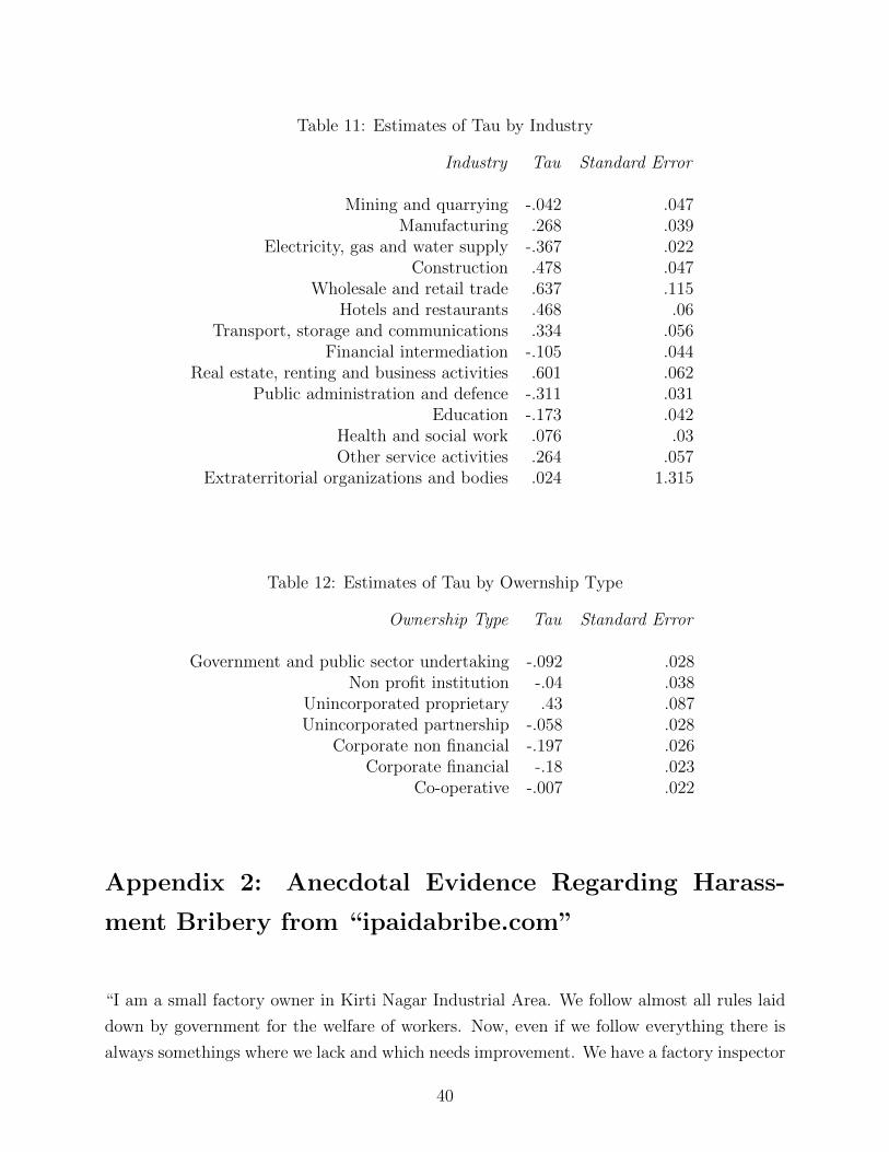
Table 11: Estimates of Tau by Industry

Industry Tau Standard Error

Mining and quarrying -.042 .047Manufacturing .268 .039

Electricity, gas and water supply -.367 .022Construction .478 .047

Wholesale and retail trade .637 .115Hotels and restaurants .468 .06

Transport, storage and communications .334 .056Financial intermediation -.105 .044

Real estate, renting and business activities .601 .062Public administration and defence -.311 .031

Education -.173 .042Health and social work .076 .03Other service activities .264 .057

Extraterritorial organizations and bodies .024 1.315

Table 12: Estimates of Tau by Owernship Type

Ownership Type Tau Standard Error

Government and public sector undertaking -.092 .028Non profit institution -.04 .038

Unincorporated proprietary .43 .087Unincorporated partnership -.058 .028

Corporate non financial -.197 .026Corporate financial -.18 .023

Co-operative -.007 .022

Appendix 2: Anecdotal Evidence Regarding Harass-

ment Bribery from “ipaidabribe.com”

“I am a small factory owner in Kirti Nagar Industrial Area. We follow almost all rules laid

down by government for the welfare of workers. Now, even if we follow everything there is

always somethings where we lack and which needs improvement. We have a factory inspector

40

by the name of Mr.R.B.Singh (M: 9818829355). He comes to all the factories in our area,

inspects them, find mistakes and then harass and blackmails us. According to him he can get

our factories sealed. To avoid this, to save our time and to save the unnecessary paperwork

we pay him every year. I have paid him twice in two years i.e. 10000 & 15000 and this is

common with all factories. Please take a strict action against him so that he learns a lesson.

I am sure he is not alone. All his colleagues are equally corrupt.”

(Reported on August 11, 2014 from New Delhi, Delhi — Report #131791)

“During the routine labor verification process by the labor department at our office, we

were advised by the consultant to pay the labor inspector a bribe to ensure that they don’t

keep calling us for needless paperwork.”

(Reported on June 28, 2011 from Chennai, Tamil Nadu — Report #35064)

“The Labour Department requires a dozen odd registers to be maintained some of them

which are totally outdated and pointless. E.g: Salary register, Attendance register, Leave

register etc.

Our IT office has an electronic system that logs all entries/exits and leave taken. We

have the records and offerred to provide it to them in a printout.

Salaries are paid electronically via bank transfer.

The officer declined and said it must be maintained in a manual register!

Finally an arrangement was made where we maintain a few records manually and the

rest he would overlook.

Cost of arrangement Rs 1500 twice a year even if the officer shows up only once a year

for the inspection!

He is supposed to inspect twice so expects to be paid even for the time he did not show

up!” (Reported on October 13, 2010 from Chennai, Tamil Nadu — Report #44950)

“Well i had gone to renew my labour license and after all the running around in the bank

and the department, the signing authority asked me to pay Rs.500 for signing. When asked

why 500, i was told since there are 5 employess for Rs.100 each.” (Reported on December

31, 2010 from Hyderabad, Andhra Pradesh — Report #43509 )

“... in my third visit i met one of office peon in Labour office he guided me for the bribe

he also investigated and advised me for bribe according to the number of Employees deployed

on contract basis and for this valueble suggestion he charged me Rs. 100. Again with full

confidence i went to the ALCs desk and straight away i offered him the packet which was

41

contains the amount of Bribe Rs. 3000/- ... He issued me the license after office hours...”

(Reported on March 30, 2011 from Mumbai, Maharashtra — Report #39133)

“Applying for shop & establishment [registration] & procured all documents relating to

the registration. Finally inspectors are asking Rs.1000 as a bribe. If any other notice received

by the company for resolving that another Rs.2000 and above , it depends on the company”

(Reported on March 28, 2014 from Bangalore, Karnataka — Report #99016)

“Officer name Naveen Kumar . Mobile no. 9468104694- He is asking for a bribe of 60,000

and is saying will issue a negative report under labour laws.” (Reported on January 24, 2014

from Gurgaon, Haryana — Report #83365)

Appendix 3: Modeling Extortion (ie: Harassment Bribery)

In this Appendix we model size-based regulations in an environment where corrupt inspectors

use the fact that de jure regulations are numerous, complex and burdensome in order to extort

bribes from firms (ie: harassment bribery). The model aims to illustrate how corruption may

lead to higher per worker costs for firms that exceed the 10 worker threshold, while being as

parsimonious as possible. The set-up and timeline is described below and in Figure 8.

First, firms must choose their number of workers (n ≥ 10 or n′ < 10).47 As in Section 4.1,

firms are characterized by a productivity parameter α, so that firms with higher productivity

would like to choose higher n. If firms choose n greater than or equal to 10, they come under

the legal purview of size-based regulations, which makes it more difficult for them to appeal

extortionary practices on the part of inspectors. After choosing a level of employment,

firms are randomly matched with an inspector. With probability κ, the inspector is corrupt;

otherwise the inspector is honest. An honest inspector will enforce a reasonable interpretation

of the spirit of the regulations if the firm has more than 10 workers. To be compliant with

this “reasonable” interpretation of the regulations will cost the firm an amount F1(n), which

may in general depend on the number of workers in the firm. A firm with fewer than 10

workers incurs no regulatory costs if matched with an honest inspector.

If the firm is instead matched with a corrupt inspector, the inspector will threaten to

report the firm for technical infractions unless it pays a bribe (which we denote b or b′,

depending on whether the firm has chosen n ≥ 10 or n′ < 10), the value of which is

47Throughout, primes will denote the values of variables on the side of the decision tree in which firmshire less than 10 workers.

42

determined by Nash Bargaining. The firm may choose to pay the bribe or appeal the

threatened fine in court. If appealing the fine in court, the firm will win with probability

p (or p′) but will incur legal fees (cL) with certainty. If it wins the case, the firm has no

further financial obligations. If the firm loses, it is obliged to pay an amount F2(n), which

we take to be much larger than F1(n). This last assumption is tantamount to supposing

that a reasonable level of compliance with regulations is not extremely costly in comparison

to the punishments that could be brought by an inspector for violating the regulations -

which may be a reasonable assumption in contexts where inspectors have a great amount of

bargaining power and/or punishments can involve prison sentences. The assumption is also

necessary for the framework to be one of extortion rather than collusion: if F1(n) were large

in comparison with F2(n), firms would benefit from collusion and would face lower costs with

corrupt inspectors than with honest ones. It is also plausible that both F2(n) and F1(n) are

increasing functions of the number of workers, especially if we acknowledge that the full cost

of any fine would include the opportunity cost of a manager’s time. We will consider the

case where the total fines are directly proportional to the number of workers: Fi(n) = fi ∗n.

The decision tree representing the firm’s choices described above is provided in Figure 8.

Figure 8: Decision Tree

Firm

n’ ¡ 10

Nature

honest inspector

π(α, n′)0

corrupt (prob κ)

Firm

pay

π(α, n′)− b′b′

appeal

Nature

win with prob p′

π(α, n′)− cL0

lose

π(α, n′)− cL − F2(n′)

0

n ≥ 10

Nature

honest inspector

π(α, n)− F1(n)0

corrupt (prob κ)

Firm

pay

π(α, n)− bb

appeal

Nature

win with prob p

π(α, n)− cL0

lose

π(α, n)− cL − F2(n)0

43

An important assumption is that p′, the probability of a firm’s winning the case when

n′ < 10, is much higher than p, the probability of winning the case when n ≥ 10. The idea

is that a firm with less than 10 workers is not under the legal purview of the regulations, so

any case regarding regulatory infractions brought against the firm would have no standing in

court. In what follows, we will take p = 0 and p′ = 1 for simplicity. As previously mentioned,

if the firm meets a corrupt inspector, the value of the bribe paid to avoid going to court is

determined through a process of Nash Bargaining over the surplus, where α and β are the

bargaining weights of the inspector and firm, respectively:

maxb

(b)α(cL + (1− p)F2(n)− b)β

The solution of this maximization problem is that b = α(cL+(1−p)F2(n))α+β

(and b′ = α(cL+(1−p′)F2(n))α+β

,

for firms with less than 10 workers). Given that firms meet corrupt inspectors (and thus pay

bribes) with probability κ and meet honest inspectors (and thus pay F1(n)) with probability

1− κ, the expected cost for a firm with greater than 10 workers is κb+ (1− κ)F1(n), while

the expected cost for a firm with less than 10 workers is κb′. Taking the difference and sub-

stituting in our expressions for b and b′, we get that firms that cross the 10 worker threshold

face an increase in expected costs of κ αα+β

(p′ − p)F2(n) + (1− κ)F1(n).

We are interested, however, in the increase in per worker costs that firms face when

exceeding the 10 worker threshold, not the increase in total costs (as discussed earlier, an

increase in per worker costs is the only way to produce a downshift in the logged firm size

distribution in a static model). Thus, we divide the last result by the number of workers,

n, to get per worker costs. Before doing so, we make the further simplifications that p = 0,

p′ = 1, α and β both equal 1 (equal bargaining weights), and that all fines are proportional

to firm size (Fi(n) = fi ∗n). Then, the increase in per worker costs for firms that exceed the

10 worker threshold is κf22

+ (1− κ)f1.

From the last result we see that if f2 � f1 (in particular, in this case, if f2 > 2f1), then

the increase in a firm’s per worker costs for exceeding the 10 worker threshold (i.e.: what we

call τ in the paper) is increasing in the proportion of corrupt inspectors, κ. Again, that we

are considering a context of extortion or “harassment bribery” is implied by the assumption

f2 � f1. It is this condition (that f2 is very large) that gives corrupt inspectors the power to

extract heavy bribes. We think it is a reasonable assumption given the anecdotal evidence

regarding bribery we have found (some of which we present in Appendix 2). To conclude, the

model above illustrates conditions that may explain the correlations we observed between

corruption and τ in Section 6. In particular, the conclusion of the model is that firms in

states with a higher proportion of corrupt inspectors (ie: more corrupt states), face higher

per worker costs for exceeding the 10 worker threshold (higher τ).

44