indiana universitykruschke/articles/kruschke2007ipamslides.pdf · locally bayesian learning john k....
TRANSCRIPT
Locally Bayesian Learning
John K. Kruschke
Indiana University
Kruschke, IPAM GSS 2007

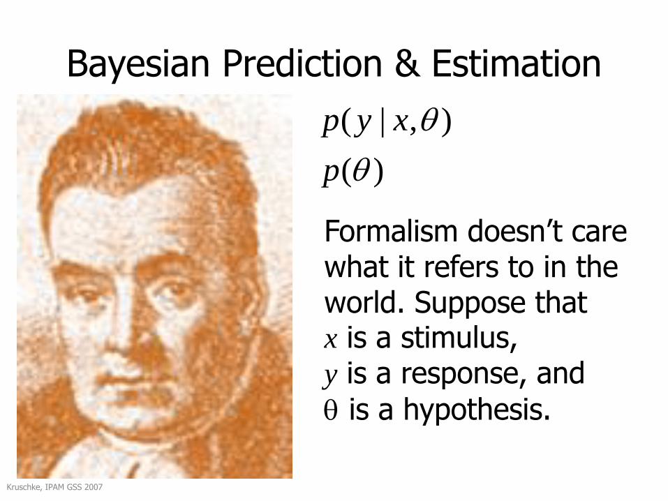
Bayesian Prediction & Estimation
),|( xyp
Hypothesized models, parameterized by , map each x value to a
probability distribution over y values.
Kruschke, IPAM GSS 2007
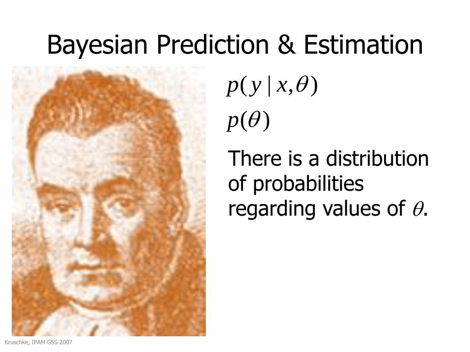
Bayesian Prediction & Estimation
),|( xyp
)(p
There is a distribution of probabilities regarding values of .
Kruschke, IPAM GSS 2007
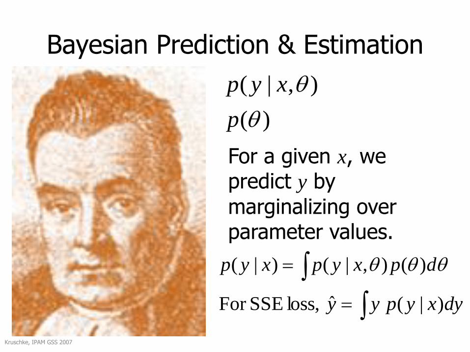
Bayesian Prediction & Estimation
),|( xyp
)(p
dyxypyy
dpxypxyp
)|( ˆ loss, SSEFor
)(),|()|(
For a given x, we predict y by
marginalizing over parameter values.
Kruschke, IPAM GSS 2007
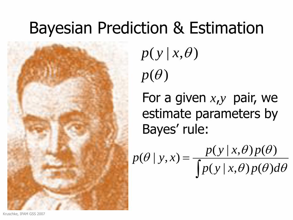
Bayesian Prediction & Estimation
dpxyp
pxypxyp
)(),|(
)(),|(),|(
),|( xyp
)(p
For a given x,y pair, we
estimate parameters by Bayes’ rule:
Kruschke, IPAM GSS 2007
Bayesian Prediction & Estimation
),|( xyp
)(p
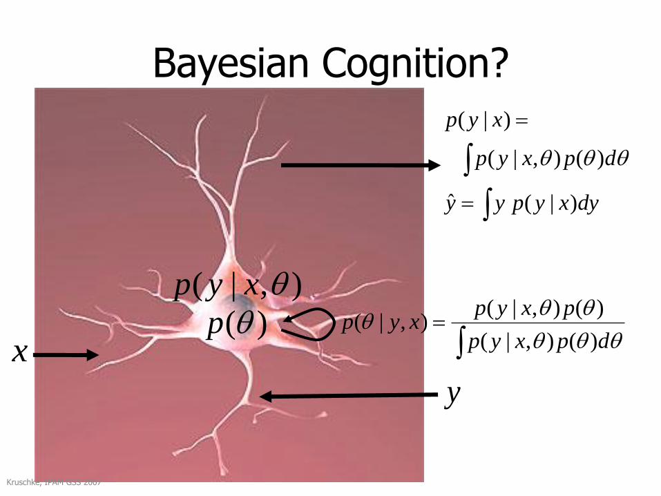
Formalism doesn’t care what it refers to in the world. Suppose thatx is a stimulus,y is a response, and
is a hypothesis.
Kruschke, IPAM GSS 2007
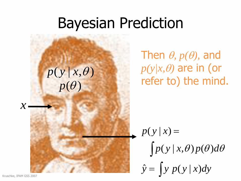
dyxypyy
dpxyp
xyp
)|( ˆ
)(),|(
)|(
Bayesian Prediction
),|( xyp
)(p
x
Kruschke, IPAM GSS 2007
Then , p(), and p(y|x,) are in (or
refer to) the mind.
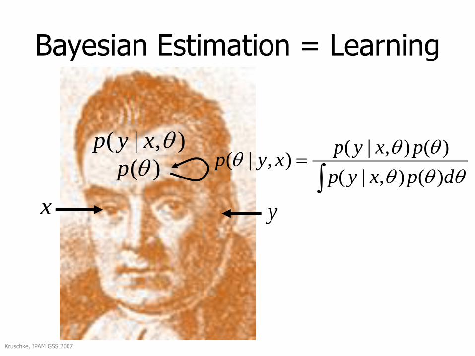
Bayesian Estimation = Learning
dpxyp
pxypxyp
)(),|(
)(),|(),|(
),|( xyp
)(p
x y
Kruschke, IPAM GSS 2007

dyxypyy
dpxyp
xyp
)|( ˆ
)(),|(
)|(
Bayesian Cognition
),|( xyp
)(p
x
dpxyp
pxypxyp
)(),|(
)(),|(),|(
y
Kruschke, IPAM GSS 2007
dyxypyy
dpxyp
xyp
)|( ˆ
)(),|(
)|(
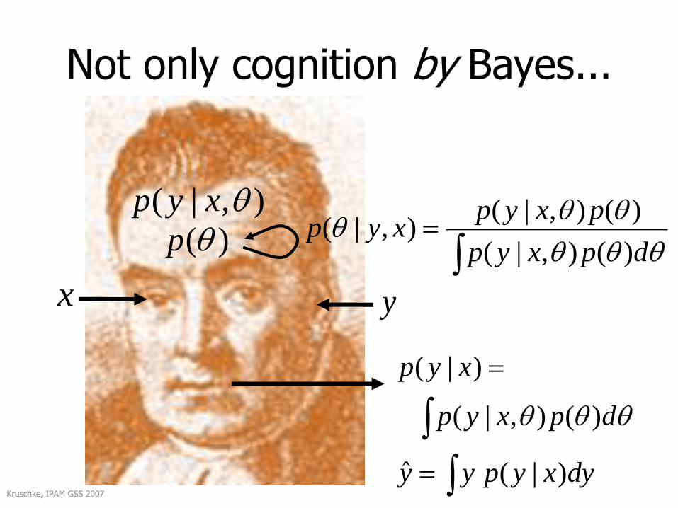
Not only cognition by Bayes...
),|( xyp
)(p
x
dpxyp
pxypxyp
)(),|(
)(),|(),|(
y
Kruschke, IPAM GSS 2007
dyxypyy
dpxyp
xyp
)|( ˆ
)(),|(
)|(
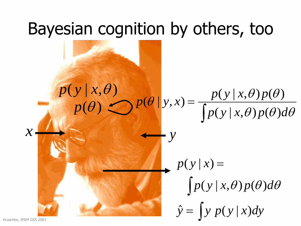
Bayesian cognition by others, too
),|( xyp
)(p
x
dpxyp
pxypxyp
)(),|(
)(),|(),|(
y
Kruschke, IPAM GSS 2007
dyxypyy
dpxyp
xyp
)|( ˆ
)(),|(
)|(
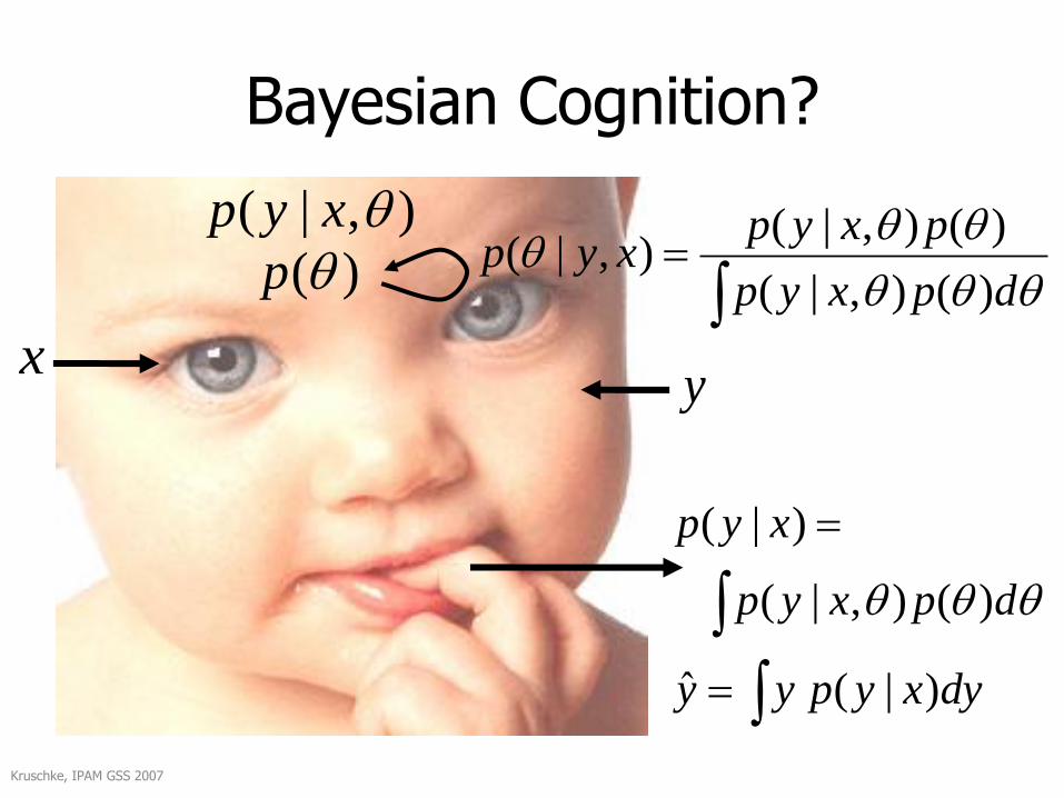
Bayesian Cognition?
),|( xyp
)(p
x
dpxyp
pxypxyp
)(),|(
)(),|(),|(
y
Kruschke, IPAM GSS 2007
dyxypyy
dpxyp
xyp
)|( ˆ
)(),|(
)|(
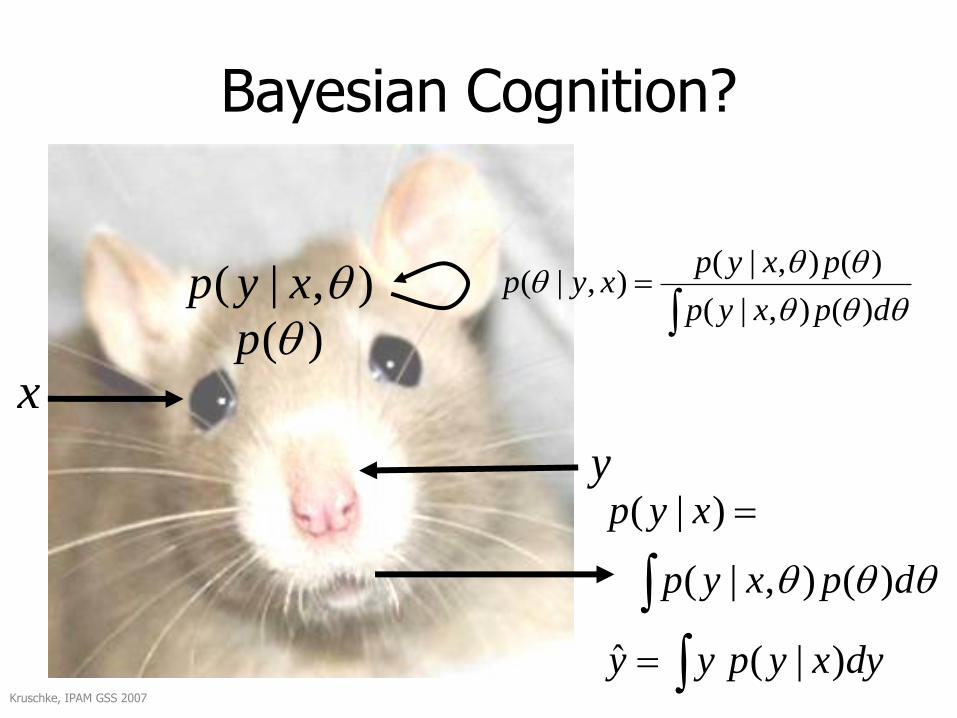
Bayesian Cognition?
),|( xyp
)(p
x
dpxyp
pxypxyp
)(),|(
)(),|(),|(
y
Kruschke, IPAM GSS 2007
dyxypyy
dpxyp
xyp
)|( ˆ
)(),|(
)|(
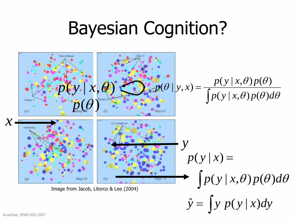
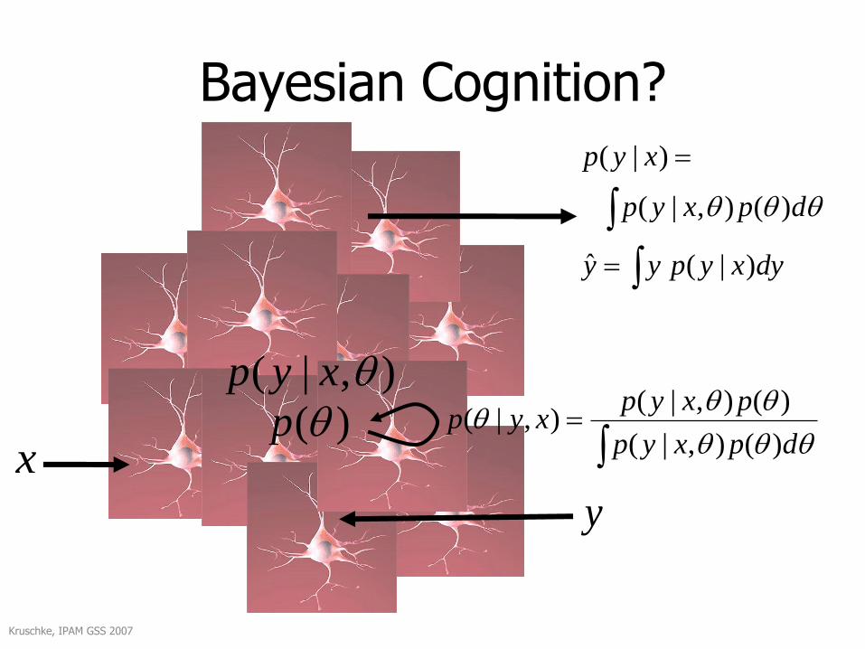
Bayesian Cognition?
),|( xyp
)(p
x
dpxyp
pxypxyp
)(),|(
)(),|(),|(
y
Kruschke, IPAM GSS 2007
Image from Jacob, Litorco & Lee (2004)
dyxypyy
dpxyp
xyp
)|( ˆ
)(),|(
)|(
Bayesian Cognition?
),|( xyp
)(px
dpxyp
pxypxyp
)(),|(
)(),|(),|(
y
Kruschke, IPAM GSS 2007
dyxypyy
dpxyp
xyp
)|( ˆ
)(),|(
)|(
Bayesian Cognition?
),|( xyp
)(px
dpxyp
pxypxyp
)(),|(
)(),|(),|(
y
Kruschke, IPAM GSS 2007

dyxypyy
dpxyp
xyp
)|( ˆ
)(),|(
)|(
Bayesian Cognition?
),|( xyp
)(p
x
dpxyp
pxypxyp
)(),|(
)(),|(),|(
y
Kruschke, IPAM GSS 2007

dyxypyy
dpxyp
xyp
)|( ˆ
)(),|(
)|(
Bayesian Cognition?
),|( xyp
)(p
x
dpxyp
pxypxyp
)(),|(
)(),|(),|(
y
Kruschke, IPAM GSS 2007
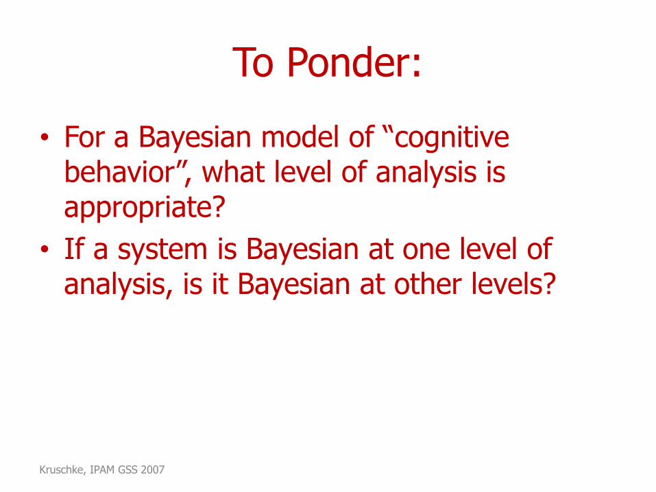
To Ponder:
• For a Bayesian model of “cognitive behavior”, what level of analysis is appropriate?
• If a system is Bayesian at one level of analysis, is it Bayesian at other levels?
Kruschke, IPAM GSS 2007

Bayesian Cognition?
Kruschke, IPAM GSS 2007
Marr (1982):
Image Intensity
Primal Sketch
2½D Sketch
3D Model
Is the overall mapping, from image to 3D model, Bayesian?
Is each component Bayesian?

Consider a Chain of Bayesians
),|( 111 xyp)( 1p
Kruschke, IPAM GSS 2007
Thomas1 Thomas2 Thomas3
),|( 222 xyp ),|( 333 xyp)( 2p )( 3p
Image Intensity
Primal Sketch
2½D Sketch
3D Model
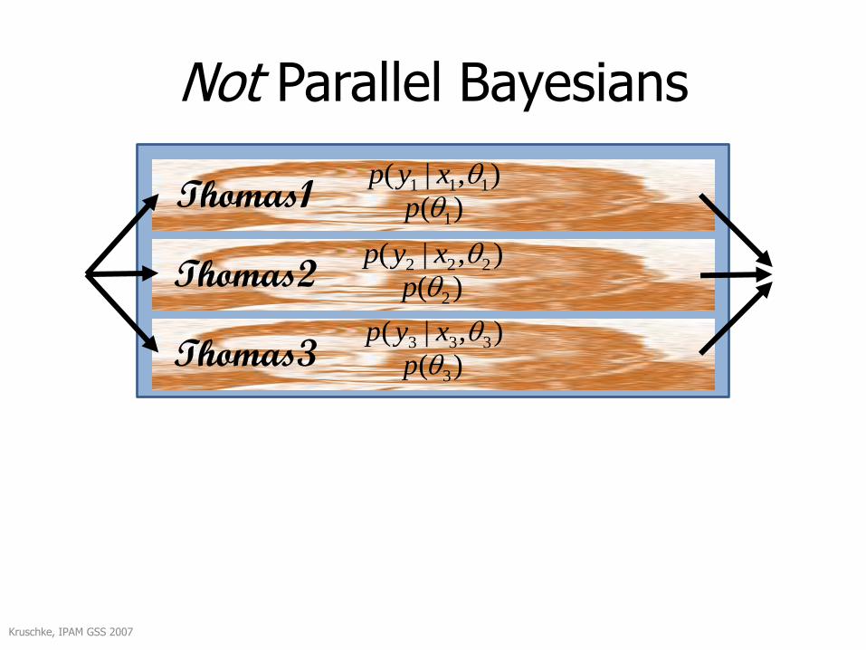
Not Parallel Bayesians
),|( 111 xyp
)( 1p
Kruschke, IPAM GSS 2007
Thomas1
),|( 222 xyp
)( 2pThomas2
),|( 333 xyp
)( 3pThomas3

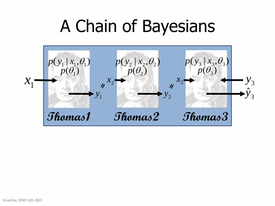
A Chain of Bayesians
),|( 111 xyp)( 1p
1x
Kruschke, IPAM GSS 2007
3y
),|( 222 xyp ),|( 333 xyp)( 2p )( 3p
1y 2y
2x 3x
Thomas1 Thomas2 Thomas3
3y
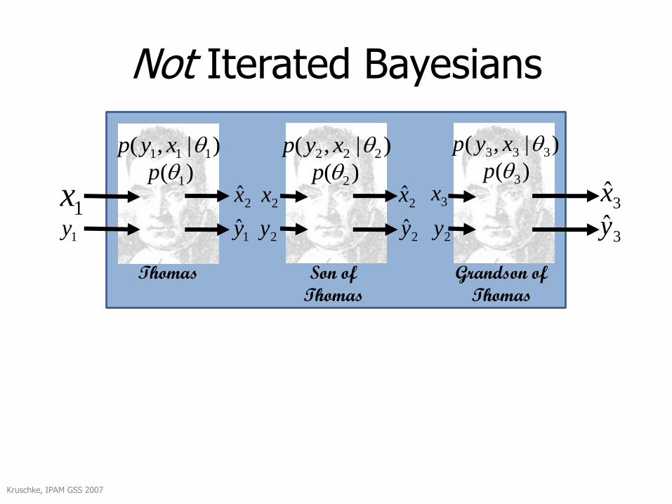
Not Iterated Bayesians
)( 1p
1x
Kruschke, IPAM GSS 2007
3y
)( 2p )( 3p
1y 2y
2x 3x
Thomas Son of
Thomas
Grandson of
Thomas
3x
)|,( 111 xyp )|,( 222 xyp )|,( 333 xyp
1y 2y 2y
2x2x
A Chain of Bayesians
),|( 111 xyp)( 1p
1x
Kruschke, IPAM GSS 2007
3y
),|( 222 xyp ),|( 333 xyp)( 2p )( 3p
1y 2y
2x 3x
Thomas1 Thomas2 Thomas3
3y
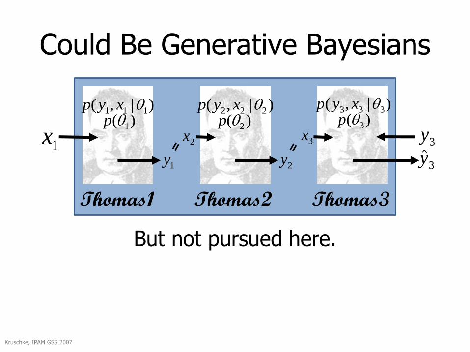
Could Be Generative Bayesians
)|,( 111 xyp)( 1p
1x
Kruschke, IPAM GSS 2007
3y
)|,( 222 xyp )|,( 333 xyp)( 2p )( 3p
1y 2y
2x 3x
Thomas1 Thomas2 Thomas3
3y
But not pursued here.

A Chain of Bayesians
),|( 111 xyp)( 1p
1x
Kruschke, IPAM GSS 2007
3y
),|( 222 xyp ),|( 333 xyp)( 2p )( 3p
1y 2y
2x 3x
Thomas1 Thomas2 Thomas3
3y
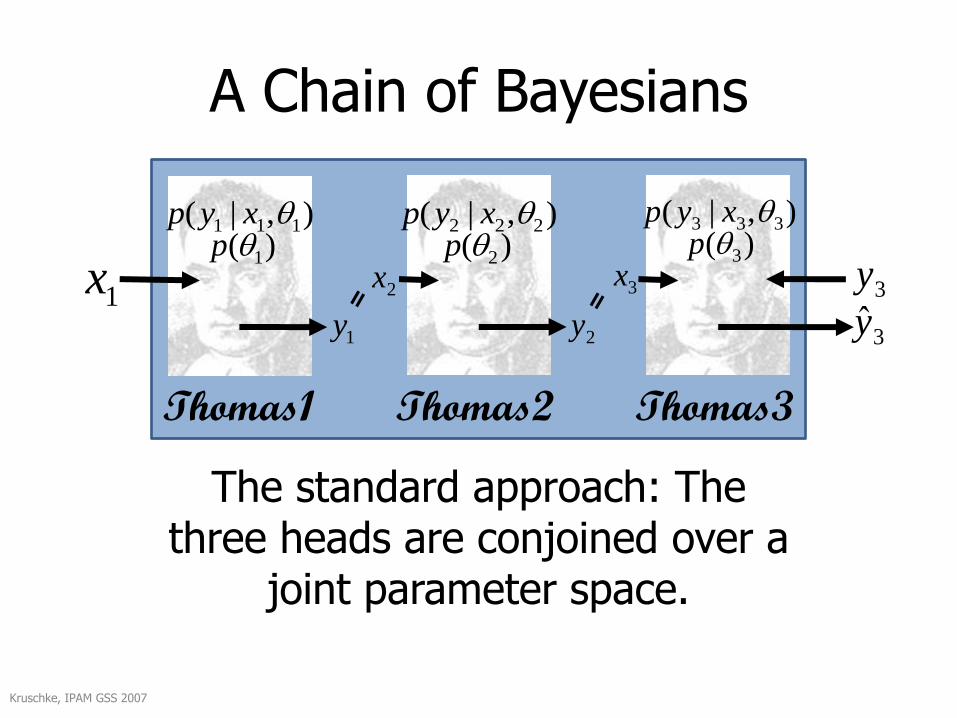
A Chain of Bayesians
),|( 111 xyp)( 1p
1x
Kruschke, IPAM GSS 2007
3y
),|( 222 xyp ),|( 333 xyp)( 2p )( 3p
1y 2y
2x 3x
Thomas1 Thomas2 Thomas3
3y
The standard approach: The three heads are conjoined over a
joint parameter space.
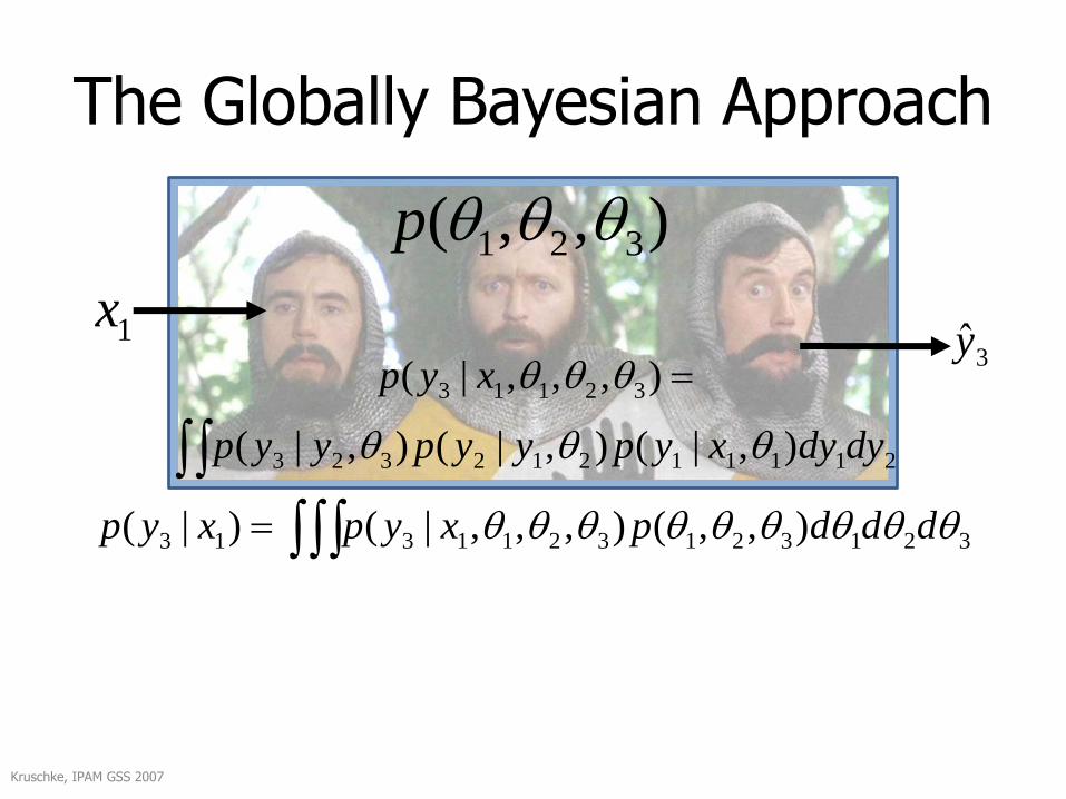
The Globally Bayesian Approach
3213213211313
21111212323
32113
),,(),,,|()|(
),|(),|(),|(
),,,|(
dddpxypxyp
dydyxypyypyyp
xyp
),,( 321 p
1x
Kruschke, IPAM GSS 2007
3y

The Globally Bayesian Approach
1x
Kruschke, IPAM GSS 2007
3y
32132132113
32132113
13321
),,(),,,|(
),,(),,,|(
),|,,(
dddpxyp
pxyp
xyp
),,( 321 p
The Locally Bayesian Approach
Kruschke, IPAM GSS 2007
You are all individuals!
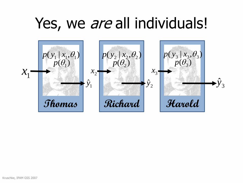
Yes, we are all individuals!
Kruschke, IPAM GSS 2007
),|( 111 xyp)( 1p
1x3y
Thomas Richard Harold
),|( 222 xyp ),|( 333 xyp)( 2p )( 3p
1y 2y
2x 3x

Locally Bayesian Prediction
),|( 111 xyp)( 1p
1x
Kruschke, IPAM GSS 2007
3y
Thomas Richard Harold
),|( 222 xyp ),|( 333 xyp)( 2p )( 3p
1y 2y
2x 3x
Each Bayesian agent computes its best prediction, and propagates it forward.
This process needs integrals over only the individual parameter spaces.
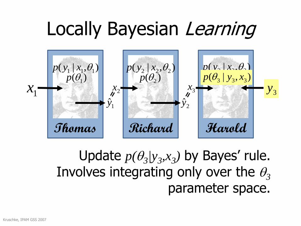
Locally Bayesian Learning
),|( 111 xyp)( 1p
1x
Kruschke, IPAM GSS 2007
3y
Thomas Richard Harold
),|( 222 xyp ),|( 333 xyp)( 2p
1y 2y
2x 3x
Update p(3|y3,x3) by Bayes’ rule. Involves integrating only over the 3
parameter space.
),|( 333 xyp

Locally Bayesian Learning
),|( 111 xyp)( 1p
1x
Kruschke, IPAM GSS 2007
3y
Thomas Richard Harold
),|( 222 xyp ),|( 333 xyp)( 2p ),|( 333 xyp
1y 2y
2x 3x
But how should poor Richard update his beliefs about 2? He needs a y2 value to
learn about!
?
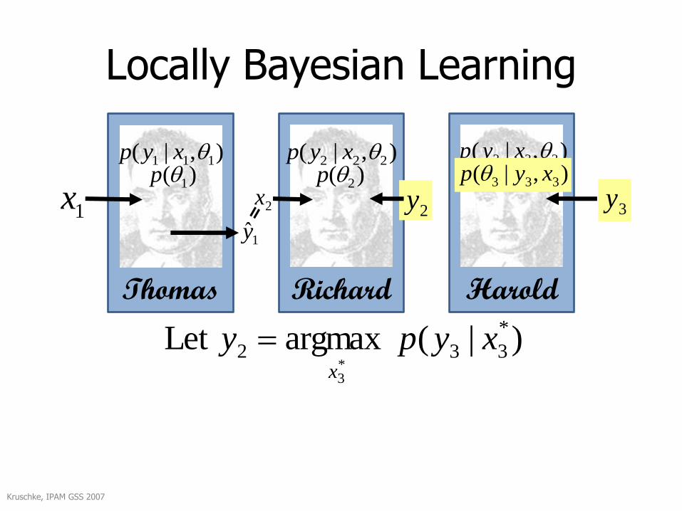
Locally Bayesian Learning
),|( 111 xyp)( 1p
1x
Kruschke, IPAM GSS 2007
3y
Thomas Richard Harold
),|( 222 xyp ),|( 333 xyp)( 2p ),|( 333 xyp
1y
2x
)|( argmaxLet *
332*3
xypyx
2y

Locally Bayesian Learning
),|( 111 xyp)( 1p
1x
Kruschke, IPAM GSS 2007
3y
Thomas Richard Harold
),|( 222 xyp ),|( 333 xyp)( 2p ),|( 333 xyp
1y
2x
)|( argmaxLet *
332*3
xypyx
2y
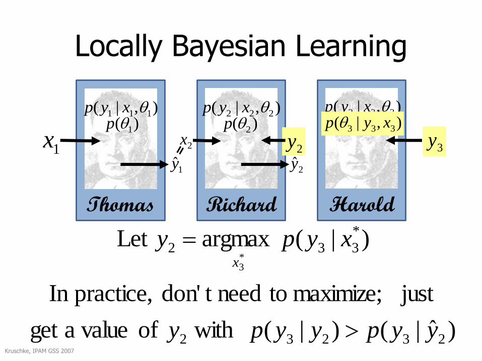
Harold tells Richard to produce a value that is consistent with Harold’s beliefs!
Locally Bayesian Learning
),|( 111 xyp)( 1p
1x
Kruschke, IPAM GSS 2007
3y
Thomas Richard Harold
),|( 222 xyp ),|( 333 xyp)( 2p ),|( 333 xyp
1y
2x
)ˆ|()|( with of a valueget
just maximize; toneedt don' practice, In
)|( argmaxLet
23232
*
332*3
yypyypy
xypyx
2y
2y

Locally Bayesian Learning
),|( 111 xyp)( 1p
1x
Kruschke, IPAM GSS 2007
3y
Thomas Richard Harold
),|( 222 xyp ),|( 333 xyp)( 2p ),|( 333 xyp
2y),|( 222 xyp
1y
)|( argmaxLet *
221*2
xypyx
?
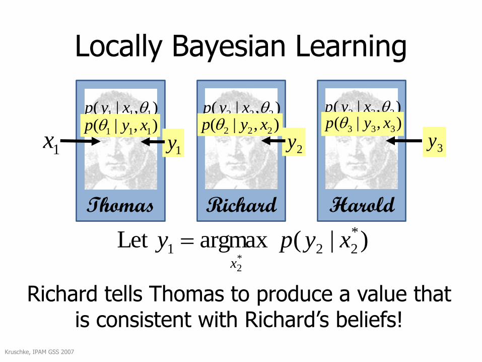
Locally Bayesian Learning
),|( 111 xyp)( 1p
1x
Kruschke, IPAM GSS 2007
3y
Thomas Richard Harold
),|( 222 xyp ),|( 333 xyp)( 2p ),|( 333 xyp
2y),|( 222 xyp
1y
)|( argmaxLet *
221*2
xypyx
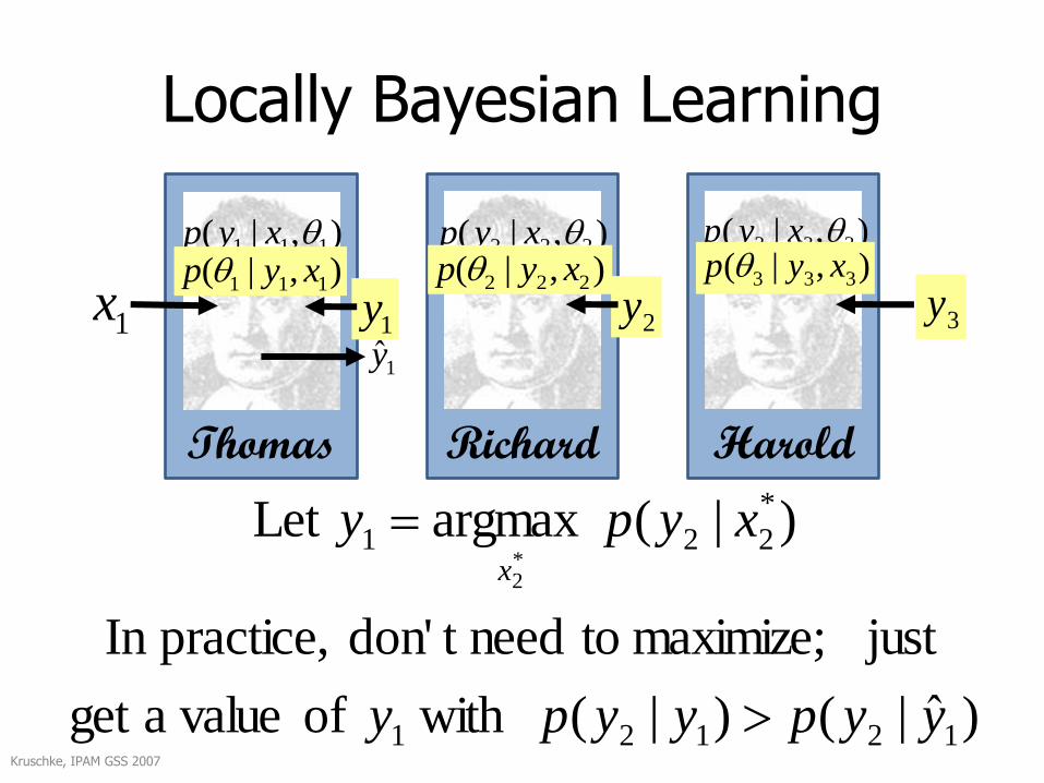
Richard tells Thomas to produce a value that is consistent with Richard’s beliefs!
),|( 111 xyp
Locally Bayesian Learning
),|( 111 xyp)( 1p
1x
Kruschke, IPAM GSS 2007
3y
Thomas Richard Harold
),|( 222 xyp ),|( 333 xyp)( 2p ),|( 333 xyp
2y),|( 222 xyp
1y
)ˆ|()|( with of a valueget
just maximize; toneedt don' practice, In
)|( argmaxLet
12121
*
221*2
yypyypy
xypyx
1y
),|( 111 xyp
Locally Bayesian Learning
),|( 111 xyp)( 1p
1x
Kruschke, IPAM GSS 2007
3y
Thomas Richard Harold
),|( 222 xyp ),|( 333 xyp)( 2p ),|( 333 xyp
2y),|( 222 xyp
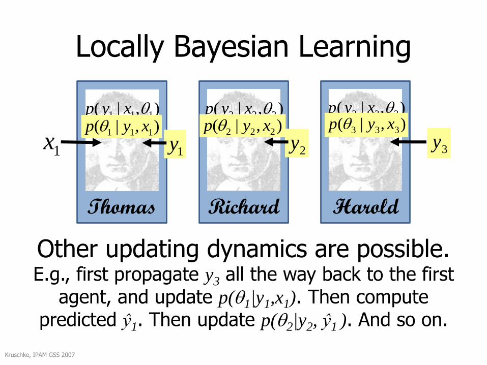
1y
Other updating dynamics are possible.E.g., first propagate y3 all the way back to the first
agent, and update p(1|y1,x1). Then compute predicted ŷ1. Then update p(2|y2, ŷ1 ). And so on.
),|( 111 xyp
Locally Bayesian Learning
),|( 111 xyp)( 1p
1x
Kruschke, IPAM GSS 2007
3y
Thomas Richard Harold
),|( 222 xyp ),|( 333 xyp)( 2p ),|( 333 xyp
2y),|( 222 xyp
1y
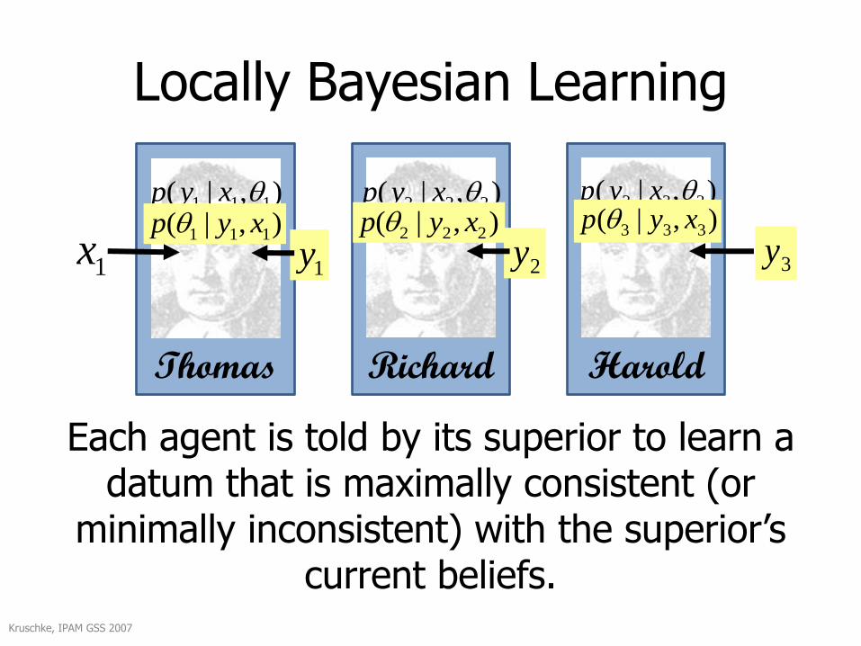
Each agent is told by its superior to learn a datum that is maximally consistent (or
minimally inconsistent) with the superior’s current beliefs.
),|( 111 xyp
Locally Bayesian Learning
),|( 111 xyp)( 1p
1x
Kruschke, IPAM GSS 2007
3y
Thomas Richard Harold
),|( 222 xyp ),|( 333 xyp)( 2p ),|( 333 xyp
2y),|( 222 xyp
1y
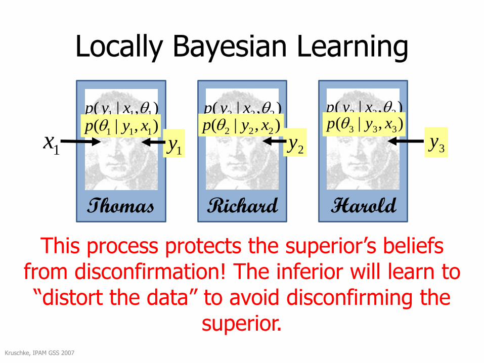
This process protects the superior’s beliefs from disconfirmation! The inferior will learn to “distort the data” to avoid disconfirming the
superior.
),|( 111 xyp
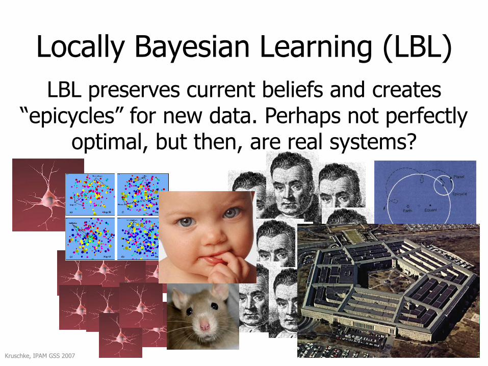
Locally Bayesian Learning (LBL)
Kruschke, IPAM GSS 2007
LBL preserves current beliefs and creates “epicycles” for new data. Perhaps not perfectly
optimal, but then, are real systems?
Put your models where your data are...
• Some real behavior, in the domain of associative learning, to which Locally Bayesian Learning can be applied.
Kruschke, IPAM GSS 2007

Typical Learning Task
RADIO
OCEAN
Press F, G, H or J.
Stimulus presentation and response collection:

Typical Learning Task
RADIO
OCEAN
[Wrong!/Correct!] The correct response is H.
Corrective feedback:

50
Phenomena Suggestive of Attention in Learning
• Fewer relevant cues faster learning.
• Intradimensional shifts are faster than extradimensional.
• Attenuated learning after blocking.
• Overshadowing.
• Context-specific attention.
• Highlighting.
• Et cetera!
51
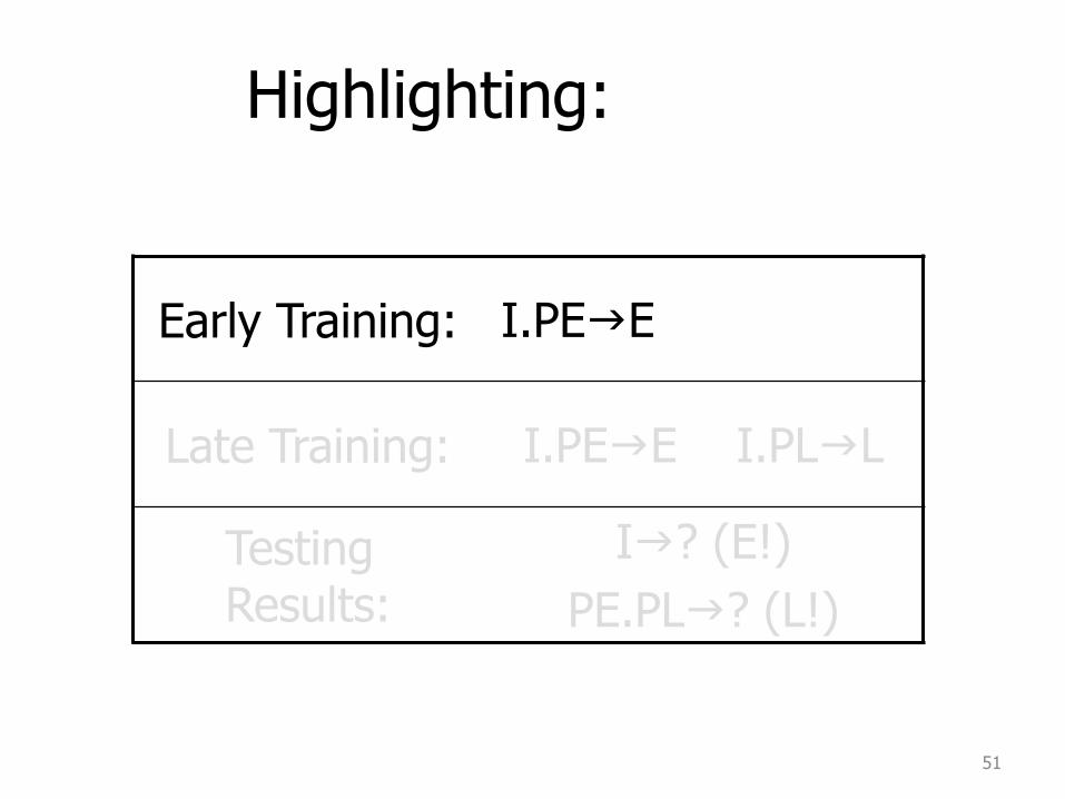
Highlighting:
Early Training: I.PEgE .
Late Training: I.PEgE I.PLgL
Testing Results:
Ig? (E!)
PE.PLg? (L!)
52
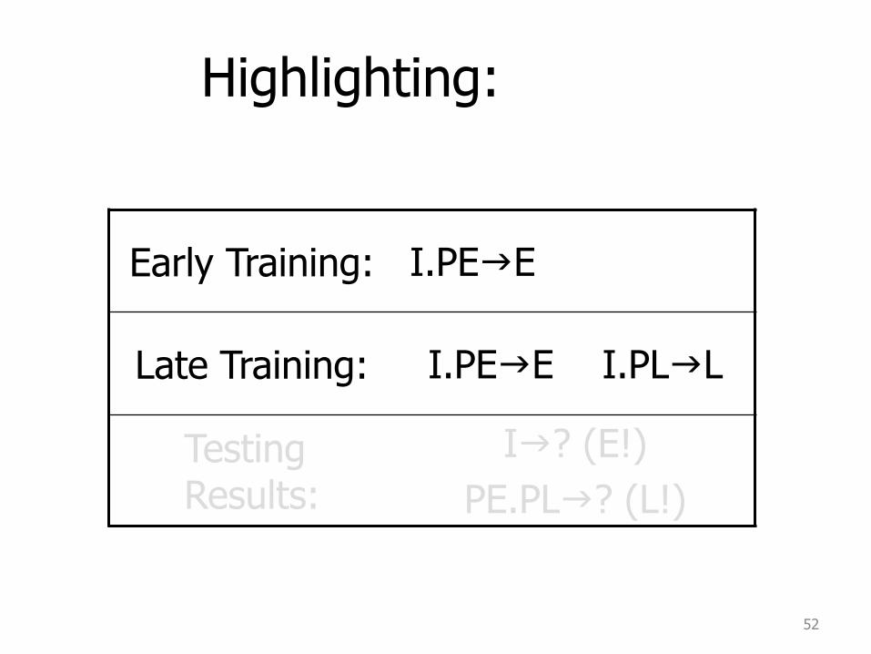
Highlighting:
Early Training: I.PEgE .
Late Training: I.PEgE I.PLgL
Testing Results:
Ig? (E!)
PE.PLg? (L!)
53
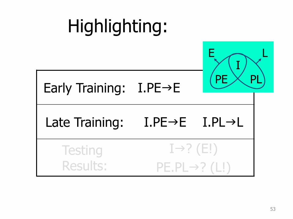
Highlighting:
Early Training: I.PEgE .
Late Training: I.PEgE I.PLgL
Testing Results:
Ig? (E!)
PE.PLg? (L!)
I
PE PL
E L

54
Highlighting:
Early Training: I.PEgE .
Late Training: I.PEgE I.PLgL
Testing Results:
Ig? (E!)
PE.PLg? (L!)
I
PE PL
E L
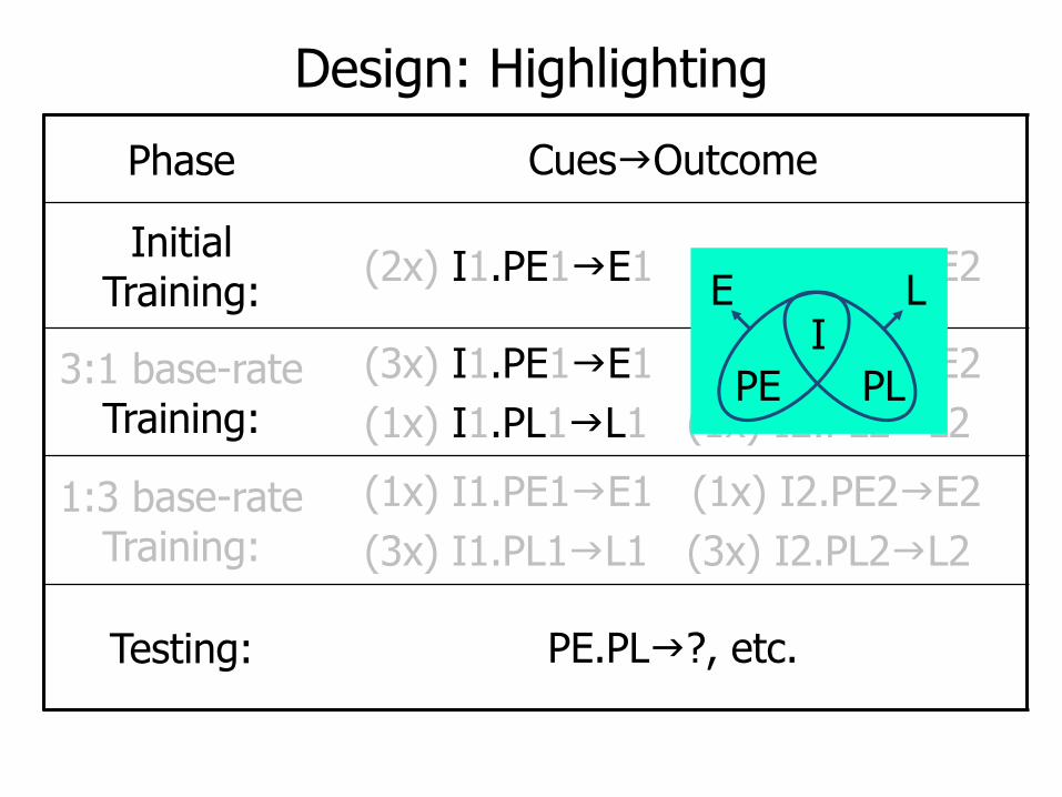
Design: Highlighting
Phase CuesgOutcome
Initial Training:
(2x) I1.PE1gE1 (2x) I2.PE2gE2
3:1 base-rateTraining:
(3x) I1.PE1gE1 (3x) I2.PE2gE2
(1x) I1.PL1gL1 (1x) I2.PL2gL2
1:3 base-rate Training:
(1x) I1.PE1gE1 (1x) I2.PE2gE2
(3x) I1.PL1gL1 (3x) I2.PL2gL2
Testing: PE.PLg?, etc.
I
PE PL
E L
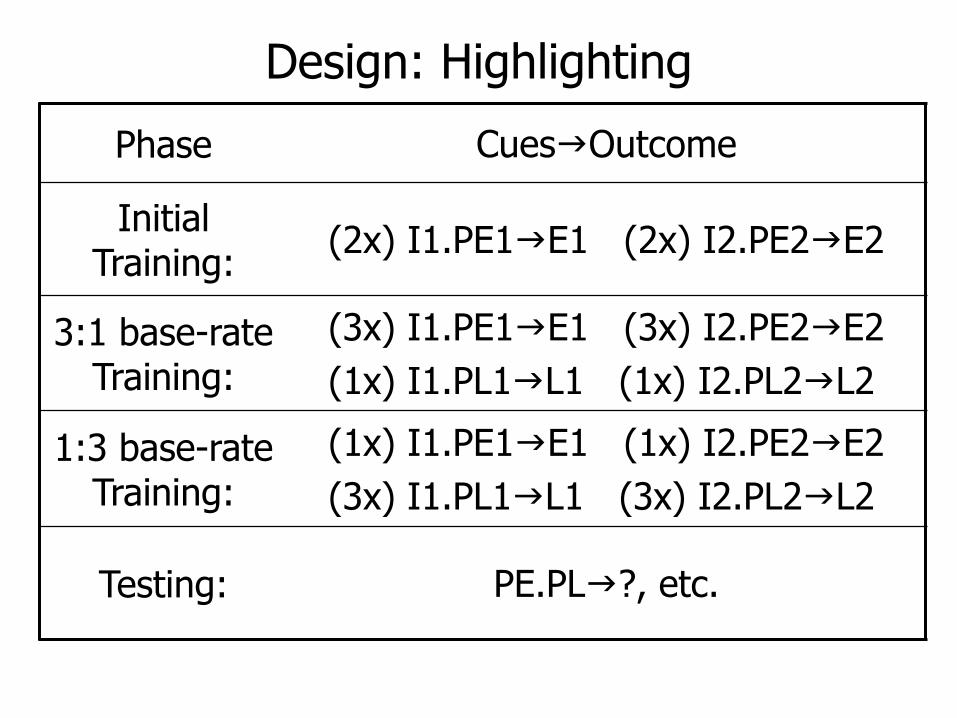
Design: Highlighting
Phase CuesgOutcome
Initial Training:
(2x) I1.PE1gE1 (2x) I2.PE2gE2
3:1 base-rate Training:
(3x) I1.PE1gE1 (3x) I2.PE2gE2
(1x) I1.PL1gL1 (1x) I2.PL2gL2
1:3 base-rate Training:
(1x) I1.PE1gE1 (1x) I2.PE2gE2
(3x) I1.PL1gL1 (3x) I2.PL2gL2
Testing: PE.PLg?, etc.
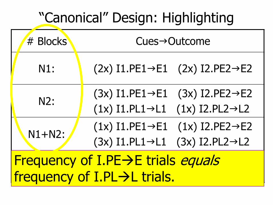
“Canonical” Design: Highlighting
# Blocks CuesgOutcome
N1: (2x) I1.PE1gE1 (2x) I2.PE2gE2
N2:(3x) I1.PE1gE1 (3x) I2.PE2gE2
(1x) I1.PL1gL1 (1x) I2.PL2gL2
N1+N2:(1x) I1.PE1gE1 (1x) I2.PE2gE2
(3x) I1.PL1gL1 (3x) I2.PL2gL2
Testing: PE.PLg?, etc.Frequency of I.PEE trials equalsfrequency of I.PLL trials.

Highlighting: Results I.PE
0
20
40
60
80
100
E L Eo Lo
I.PE
I
PE PL
E L
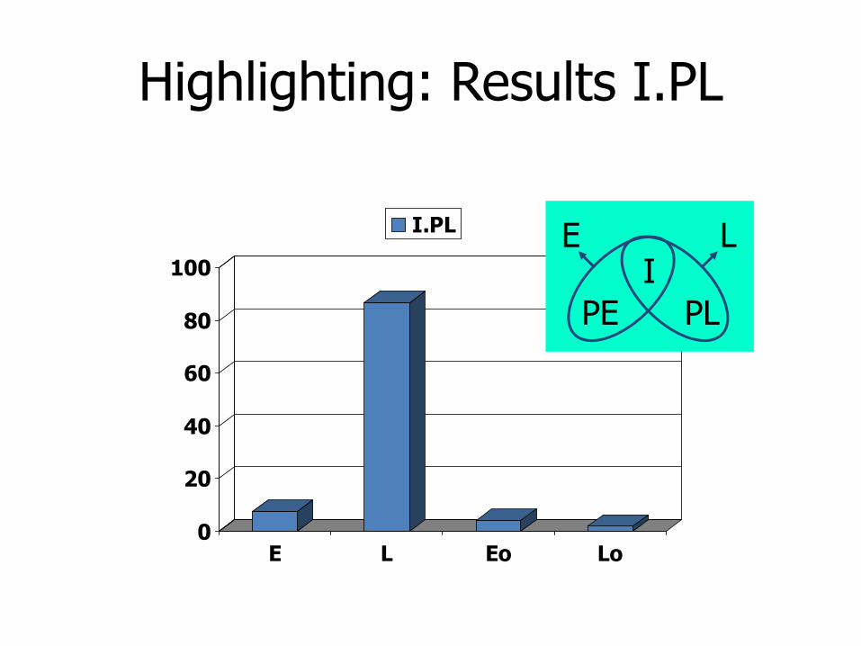
Highlighting: Results I.PL
0
20
40
60
80
100
E L Eo Lo
I.PL
I
PE PL
E L
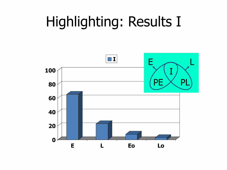
Highlighting: Results I
0
20
40
60
80
100
E L Eo Lo
I
I
PE PL
E L
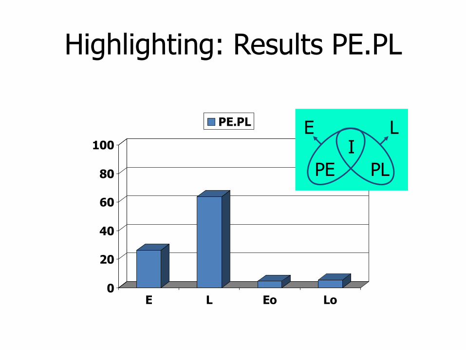
Highlighting: Results PE.PL
0
20
40
60
80
100
E L Eo Lo
PE.PL
I
PE PL
E L

Highlighting: Results I.PE.PL
0
20
40
60
80
100
E L Eo Lo
I.PE.PL
I
PE PL
E L
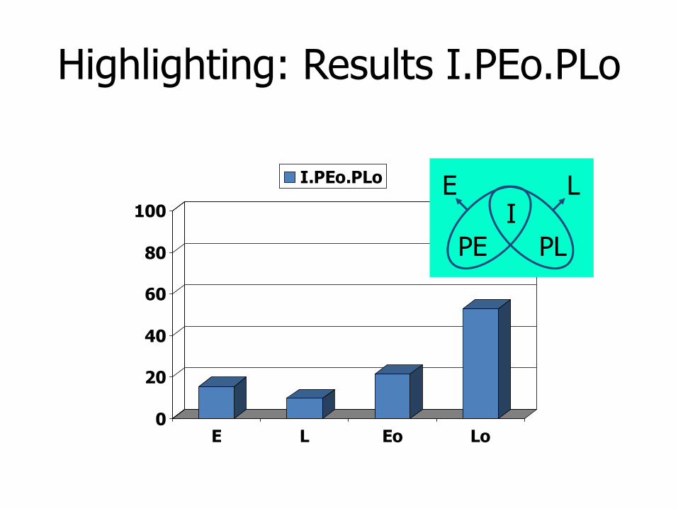
Highlighting: Results I.PEo.PLo
0
20
40
60
80
100
E L Eo Lo
I.PEo.PLo
I
PE PL
E L

64
Not just for meaningless associations...
• Highlighting also happens in meaningful domains...
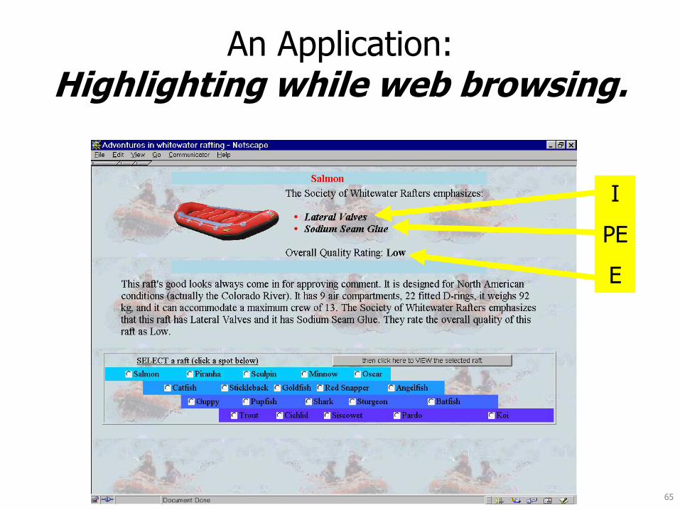
65
I
PE
E
An Application: Highlighting while web browsing.
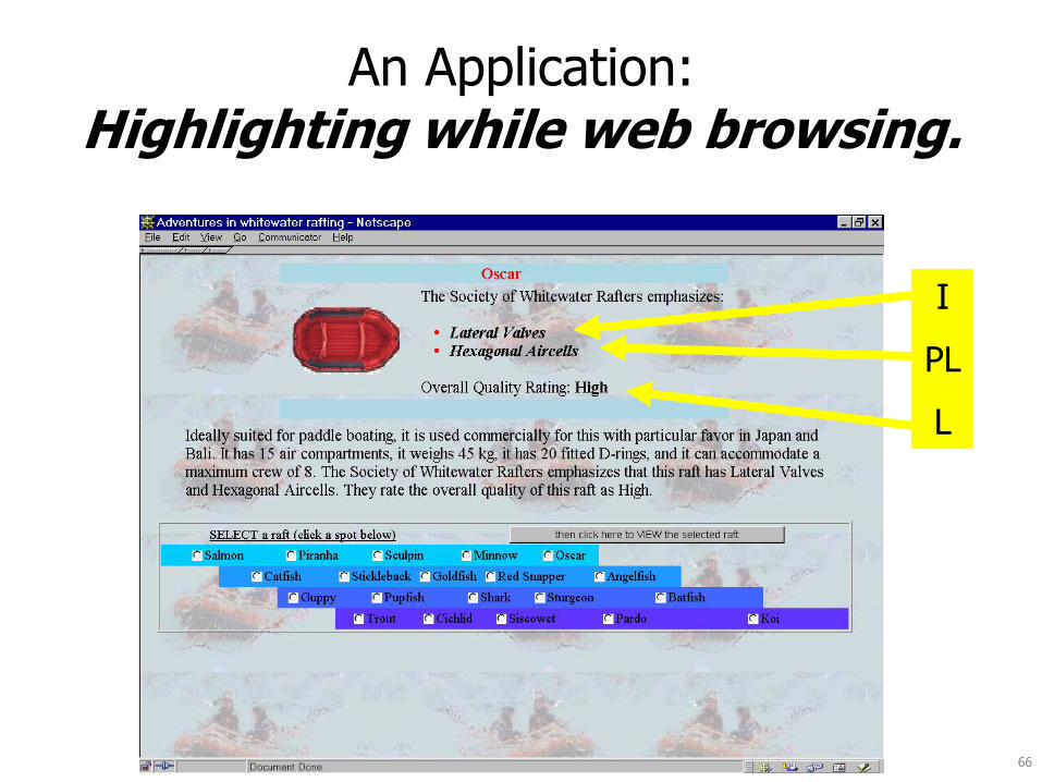
66
I
PL
L
An Application: Highlighting while web browsing.
67
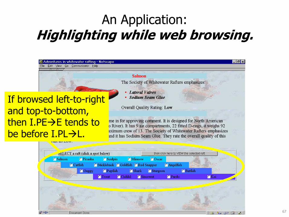
An Application: Highlighting while web browsing.
If browsed left-to-right and top-to-bottom, then I.PEE tends to be before I.PLL.

68
Test items
PE
PL
Results: I yields strong preference for Early quality;PE.PL yields strong preference for Later quality.
69
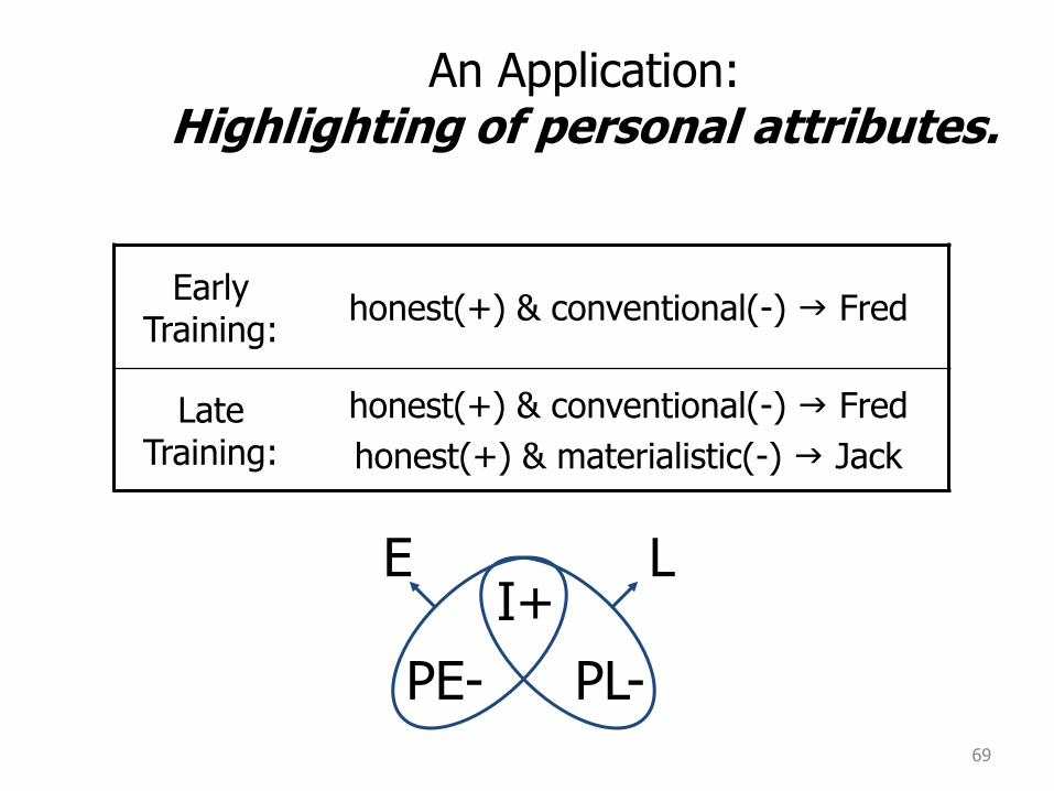
An Application: Highlighting of personal attributes.
Early Training:
honest(+) & conventional(-) g Fred
Late Training:
honest(+) & conventional(-) g Fred
honest(+) & materialistic(-) g Jack
I+
PE- PL-
E L
70
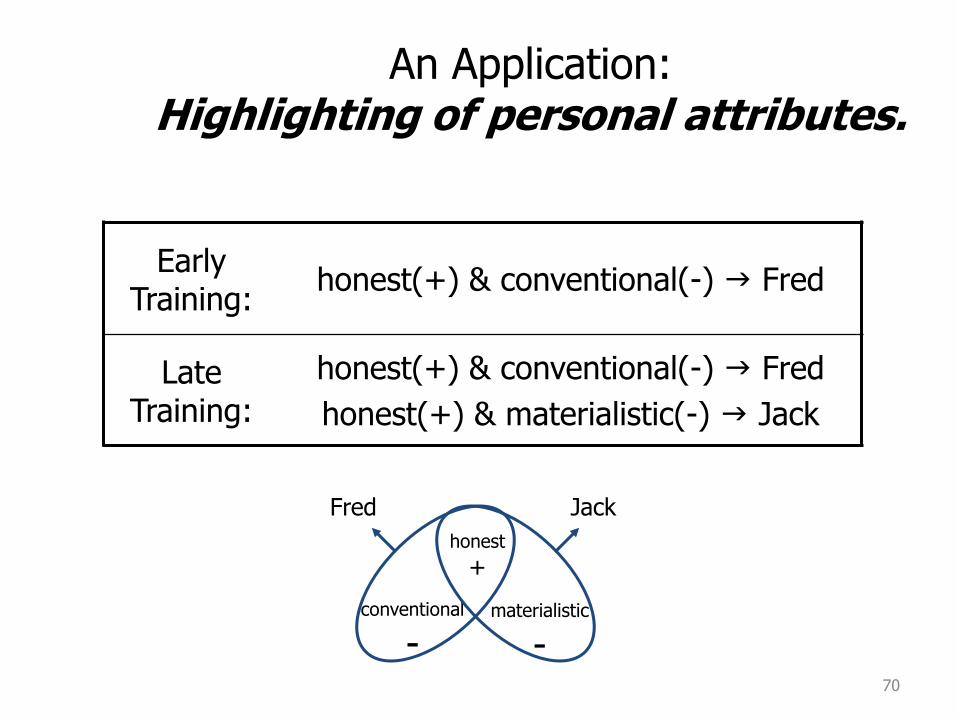
An Application: Highlighting of personal attributes.
Early Training:
honest(+) & conventional(-) g Fred
Late Training:
honest(+) & conventional(-) g Fred
honest(+) & materialistic(-) g Jack
honest
+
conventional
-materialistic
-
Fred Jack
71
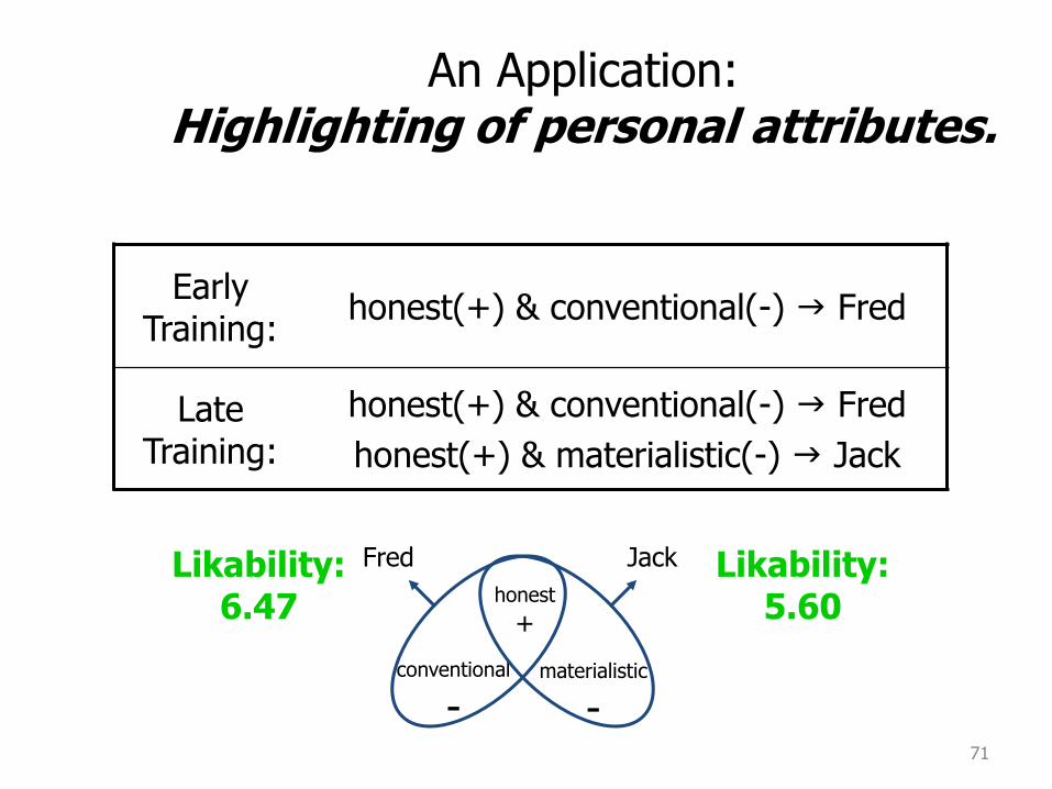
An Application: Highlighting of personal attributes.
Early Training:
honest(+) & conventional(-) g Fred
Late Training:
honest(+) & conventional(-) g Fred
honest(+) & materialistic(-) g Jack
honest
+
conventional
-materialistic
-
Fred Jack Likability: 5.60
Likability: 6.47
72
What causes highlighting?
• Can your favorite model of learning account for highlighting?
• How about various Bayesian approaches?
– Only candidates are Bayesian approaches with sensitivity to time or trial order
Rational Model(J. R. Anderson 1990)
• Representation:– There are internal clusters that represent subsets of
training items.
– Each cluster has its own set of Dirichlet distributions over beliefs about feature probabilities.
• Learning:– For each item presented, the item is assigned to the
cluster that is most probable.
– The Dirichlet parameters of that cluster are Bayesian updated.
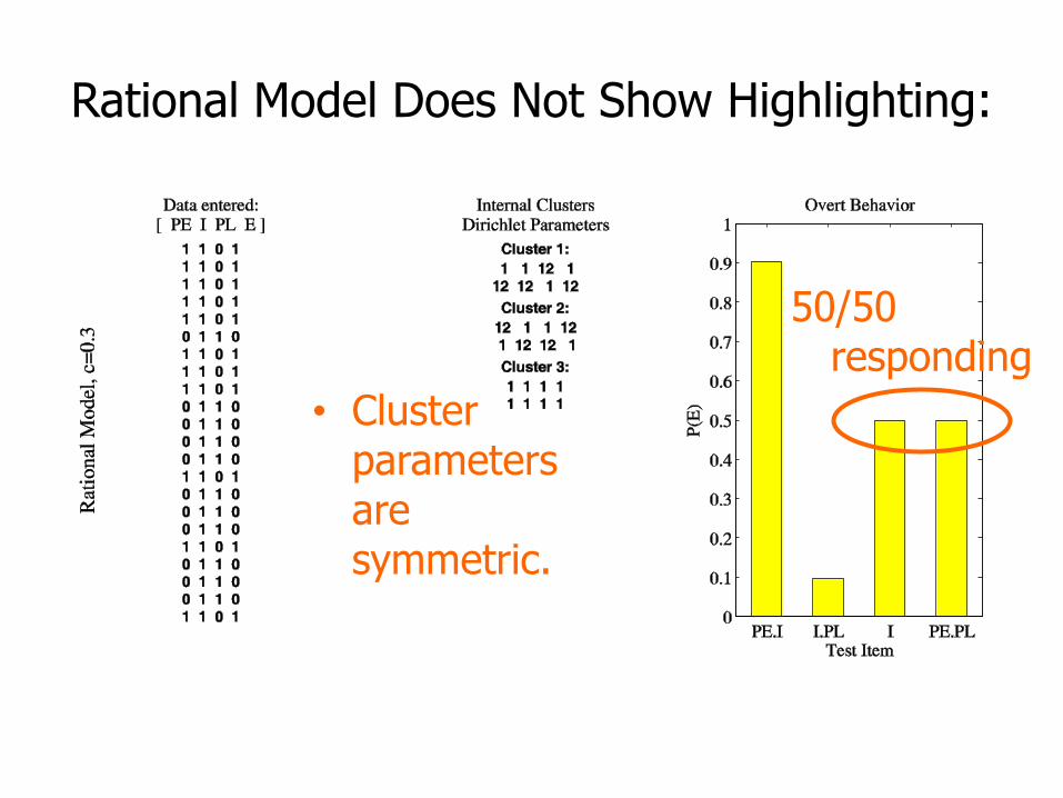
Rational Model Does Not Show Highlighting:
• Cluster parameters are symmetric.
50/50 responding

i
cue
ii
out awa
cuea2
2w1w
cuea1
Kalman Filter(Sutton 1992; Dayan, Kakade et al. 2000+)
CwNwp ,|~
vatNtp out,|~
cuea2
2w1w
cuea1
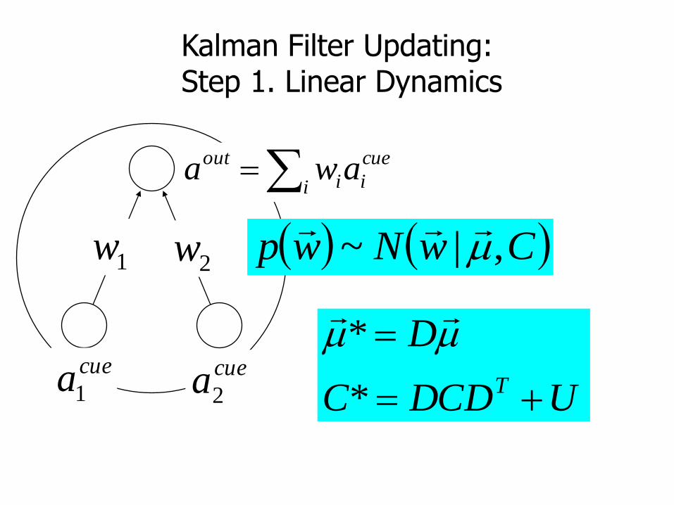
Kalman Filter Updating: Step 1. Linear Dynamics
CwNwp ,|~
i
cue
ii
out awa
UDCDC
D
T
*
*

cuea2
2w1w
cuea1
Kalman Filter Updating: Step 2. Bayesian Learning
****'
***'
1
1
CaaCavaCCC
ataCavaC
TcuecueTcuecue
TcuecueTcuecue
**,|~ CwNwp
i
cue
ii
out awa
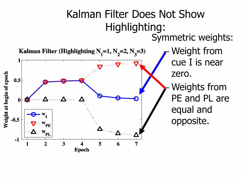
Kalman Filter Does Not Show Highlighting:
Symmetric weights:
– Weight from cue I is near zero.
– Weights from PE and PL are equal and opposite.

Explanation of Highlighting:
• Attention rapidly shifts to the distinctive feature of the later learned outcome.
I
PE PL
E L
Taught:
I
PE PL
E L
Learned:
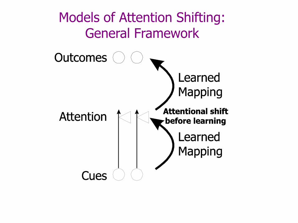
Models of Attention Shifting: General Framework
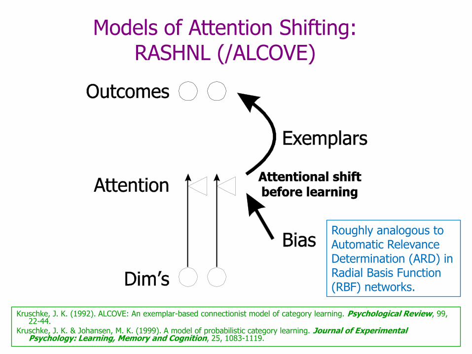
Kruschke, J. K. (1992). ALCOVE: An exemplar-based connectionist model of category learning. Psychological Review, 99, 22-44.
Kruschke, J. K. & Johansen, M. K. (1999). A model of probabilistic category learning. Journal of Experimental Psychology: Learning, Memory and Cognition, 25, 1083-1119.
Models of Attention Shifting: RASHNL (/ALCOVE)
Roughly analogous to Automatic Relevance Determination (ARD) in Radial Basis Function (RBF) networks.

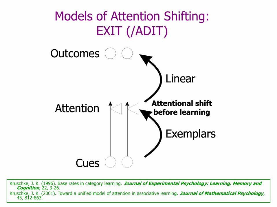
Models of Attention Shifting: EXIT (/ADIT)
Kruschke, J. K. (1996). Base rates in category learning. Journal of Experimental Psychology: Learning, Memory and Cognition, 22, 3-26.
Kruschke, J. K. (2001). Toward a unified model of attention in associative learning. Journal of Mathematical Psychology, 45, 812-863.
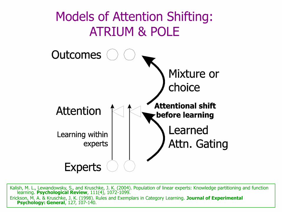
Models of Attention Shifting: ATRIUM & POLE
Kalish, M. L., Lewandowsky, S., and Kruschke, J. K. (2004). Population of linear experts: Knowledge partitioning and functionlearning. Psychological Review, 111(4), 1072-1099.
Erickson, M. A. & Kruschke, J. K. (1998). Rules and Exemplars in Category Learning. Journal of Experimental Psychology: General, 127, 107-140.

Models of Attention Shifting: Locally Bayesian
Kruschke, J. K. (2006). Locally Bayesian learning with applications to retrospective revaluation and highlighting. Psychological Review, 113, 677-699.
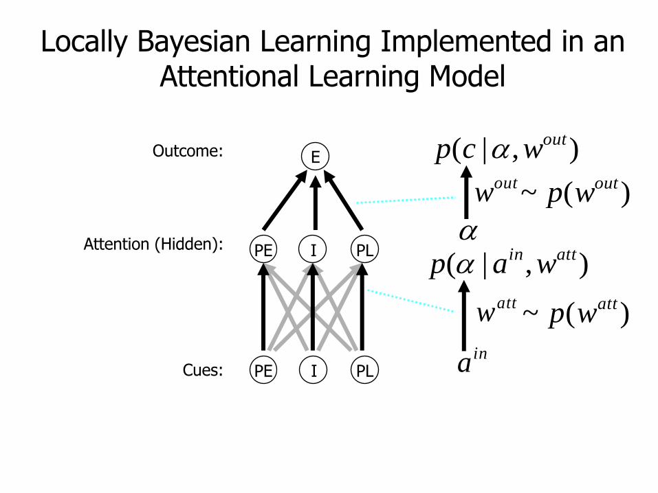
Locally Bayesian Learning Implemented in an Attentional Learning Model
Cues:
Attention (Hidden):
Outcome:
),|( attin wap attw )(~ attwp
ina
outw )(~ outwp
),|( outwcp
E
PE I PL
PE I PL
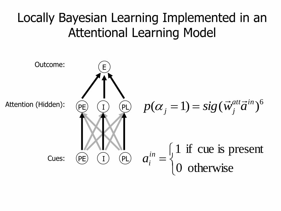
Locally Bayesian Learning Implemented in an Attentional Learning Model
Cues:
Attention (Hidden):
Outcome:
6)()1( inatt
jj awsigp
otherwise 0
present is cue if 1in
ia
E
PE I PL
PE I PL
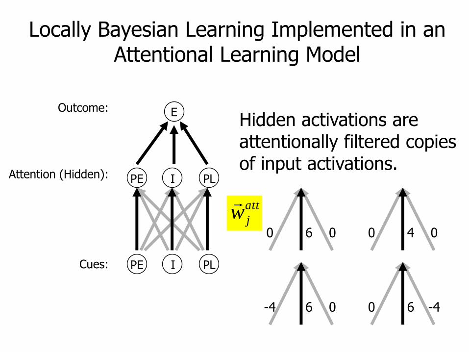
Locally Bayesian Learning Implemented in an Attentional Learning Model
Cues:
Attention (Hidden):
Outcome: E
PE I PL
PE I PL
Hidden activations are attentionally filtered copies of input activations.
6 00 4 00
6 0-4 6 -40
att
jw
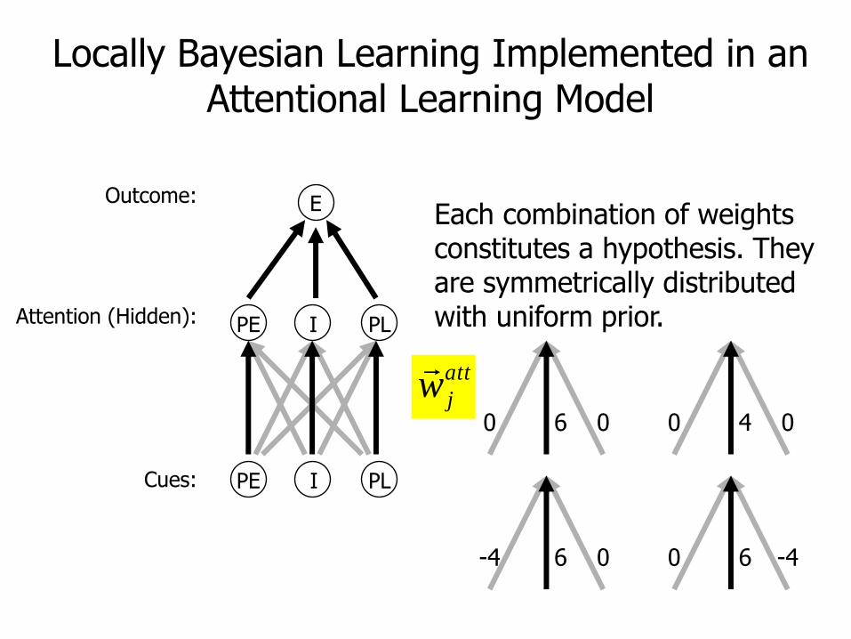
Locally Bayesian Learning Implemented in an Attentional Learning Model
Cues:
Attention (Hidden):
Outcome: E
PE I PL
PE I PL
Each combination of weights constitutes a hypothesis. They are symmetrically distributed with uniform prior.
6 00 4 00
6 0-4 6 -40
att
jw
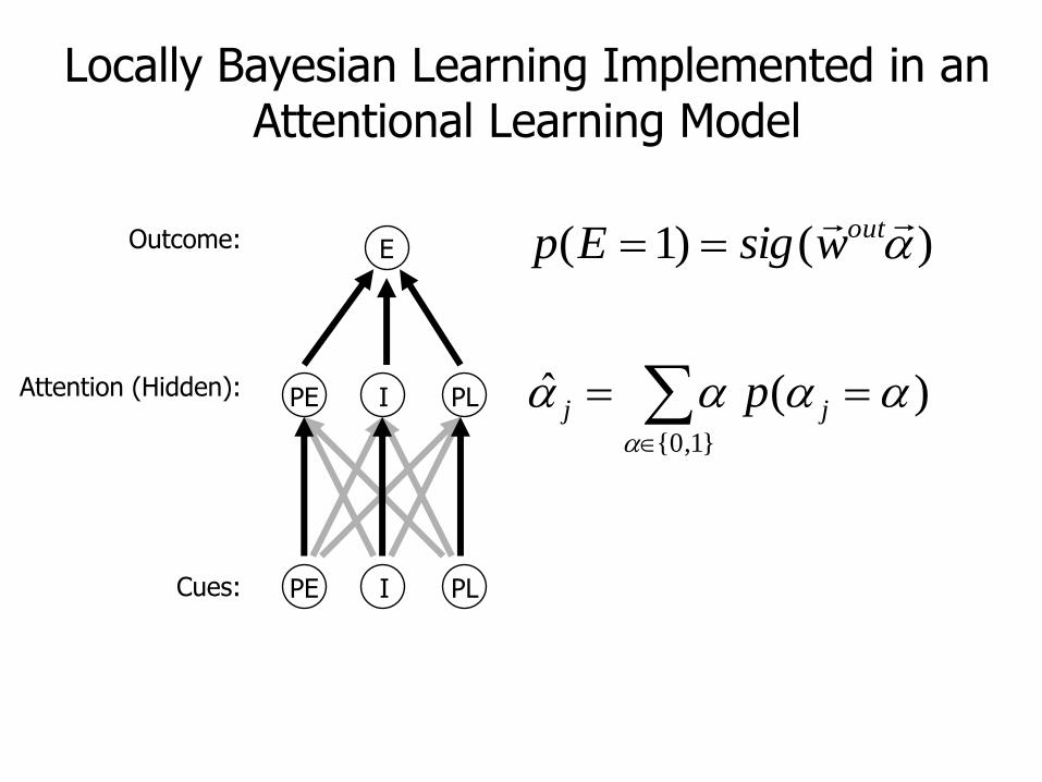
Locally Bayesian Learning Implemented in an Attentional Learning Model
Cues:
Attention (Hidden):
Outcome: E
PE I PL
PE I PL
)()1( outwsigEp
}1,0{
)( ˆ
jj p
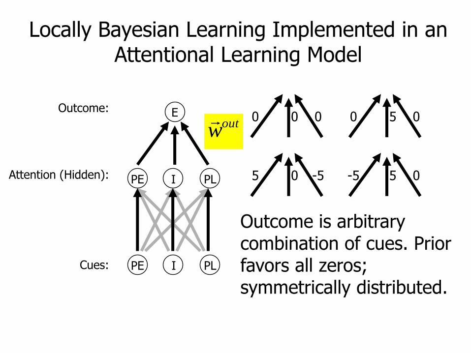
Locally Bayesian Learning Implemented in an Attentional Learning Model
Cues:
Attention (Hidden):
Outcome: E
PE I PL
PE I PL
Outcome is arbitrary combination of cues. Prior favors all zeros; symmetrically distributed.
0 00 5 00
0 -55 5 0-5
outw
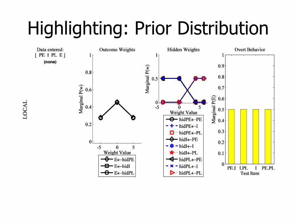
Highlighting: Prior Distribution
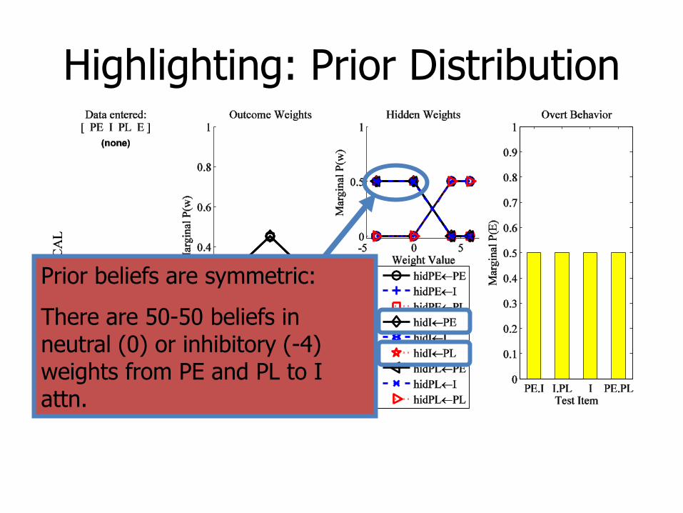
Highlighting: Prior Distribution
Prior beliefs are symmetric:
There are 50-50 beliefs in neutral (0) or inhibitory (-4) weights from PE and PL to I attn.
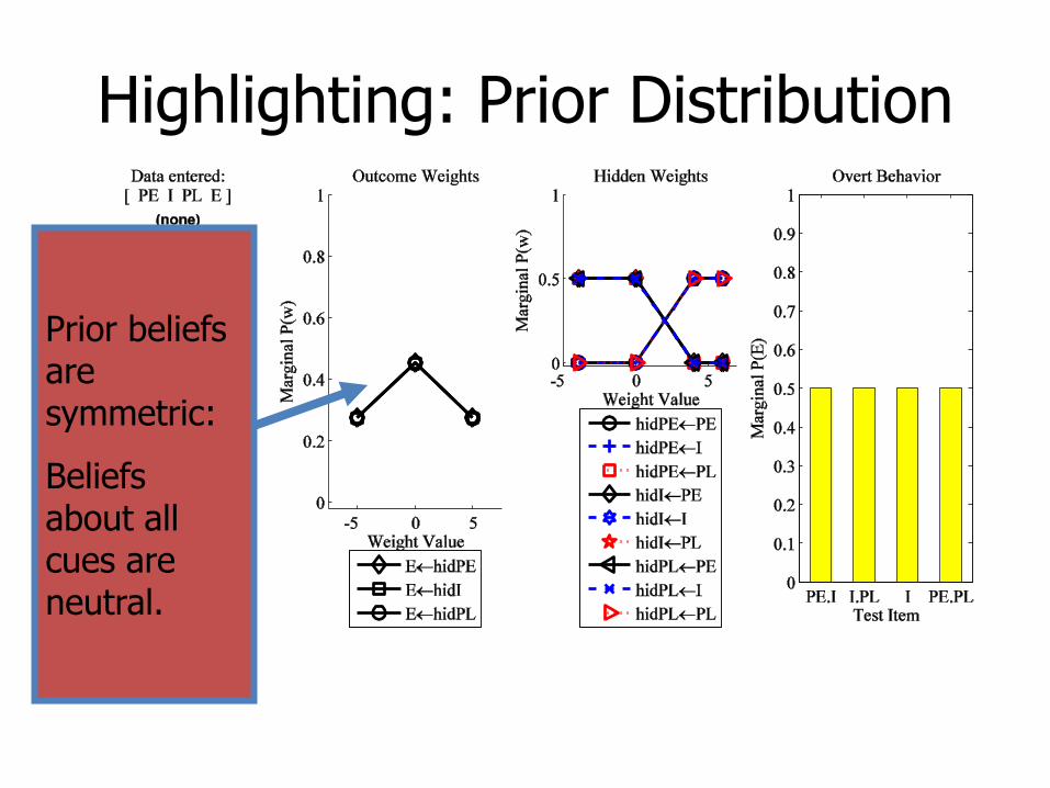
Highlighting: Prior Distribution
Prior beliefs are symmetric:
Beliefs about all cues are neutral.

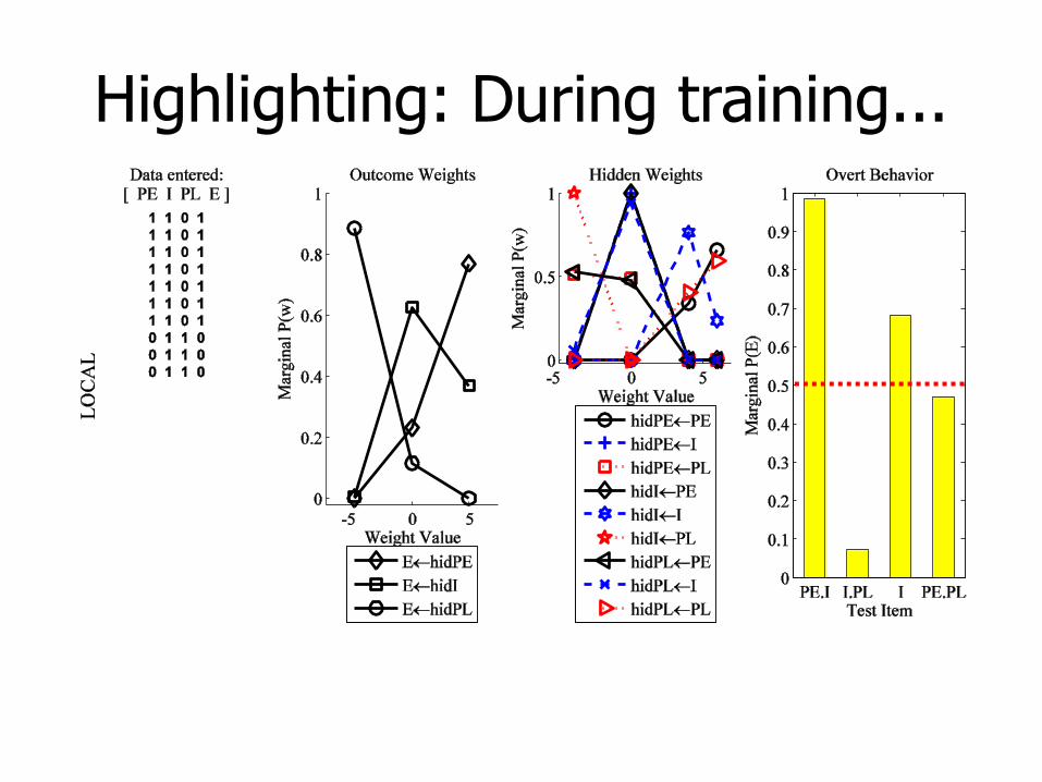
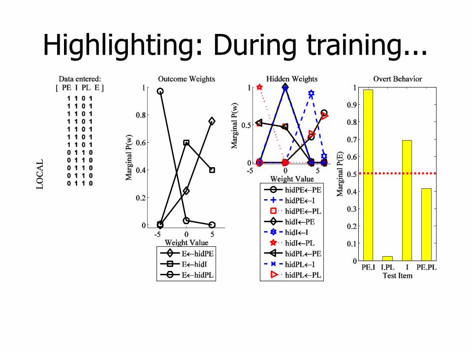
Highlighting: During training...
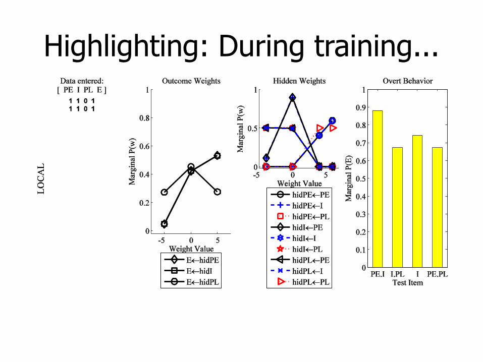
Highlighting: During training...

Highlighting: During training...

Highlighting: During training...
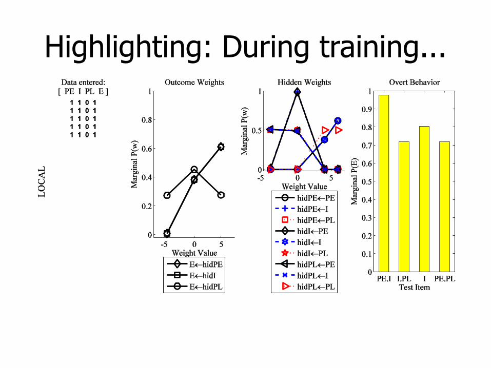
Highlighting: During training...

Highlighting: During training...
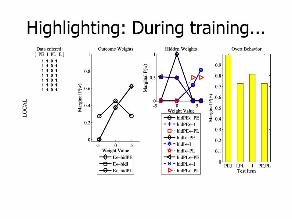
Highlighting: During training...
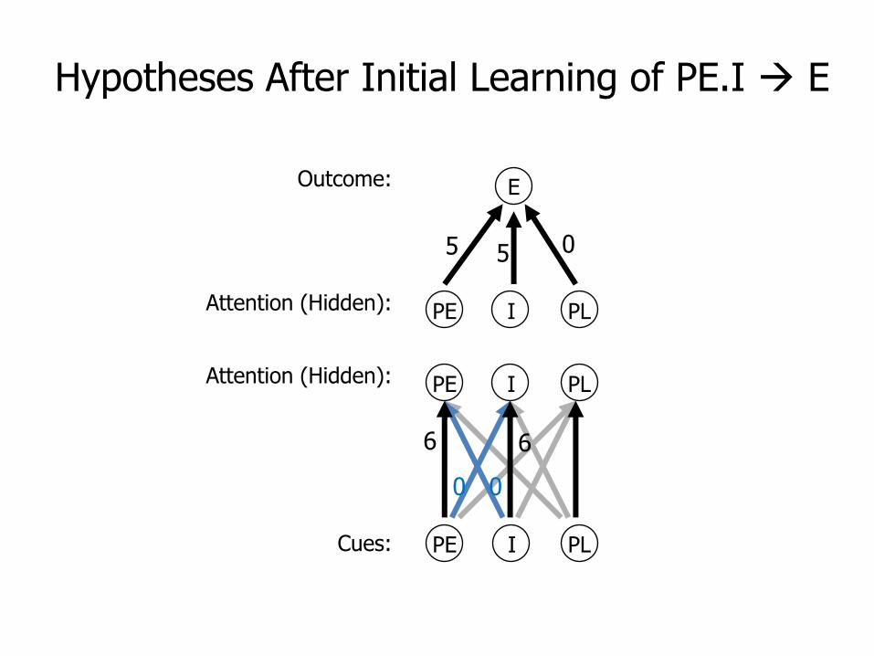
Hypotheses After Initial Learning of PE.I E
Cues:
Attention (Hidden):
Outcome: E
PE I PL
PE I PL
5 5 0
00
6 6
Attention (Hidden): PE I PL
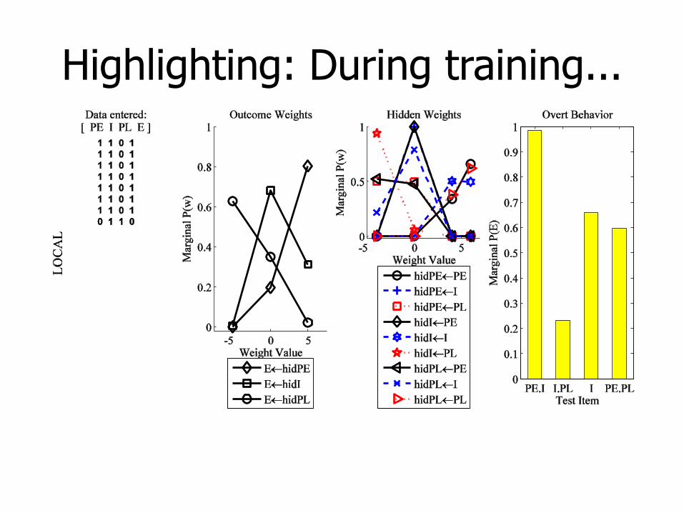
Highlighting: During training...

Highlighting: During training...
Highlighting: During training...

Highlighting: During training...
Highlighting: During training...
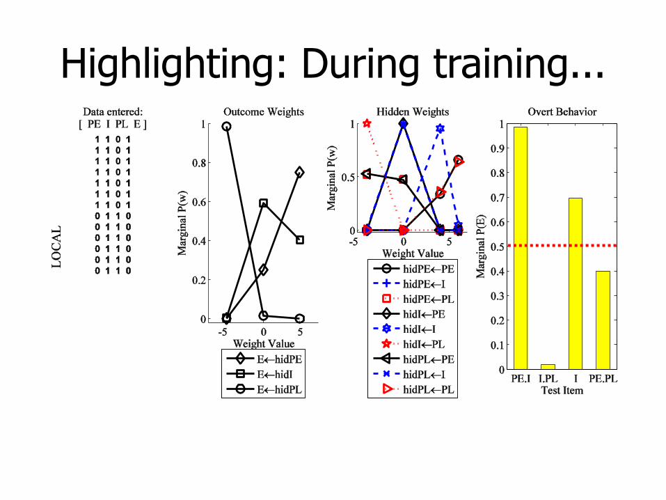
Highlighting: During training...
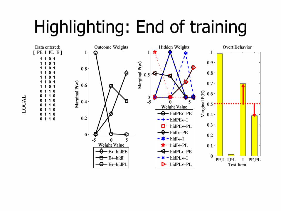
Highlighting: End of training
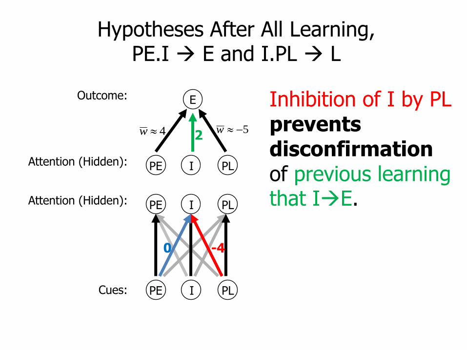
Hypotheses After All Learning, PE.I E and I.PL L
Cues:
Attention (Hidden):
Outcome: E
PE I PL
PE I PL
-40
5w4w
Attention (Hidden): PE I PL
Inhibition of I by PL prevents disconfirmation of previous learning that IE.
2
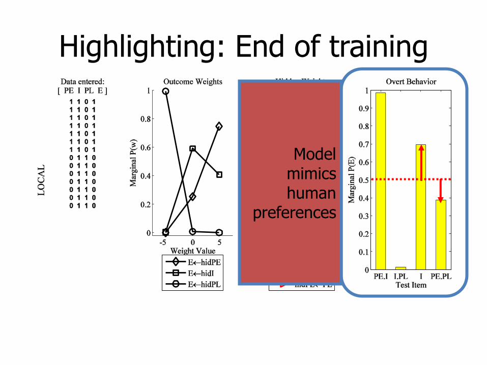
Highlighting: End of training
Model mimics human
preferences
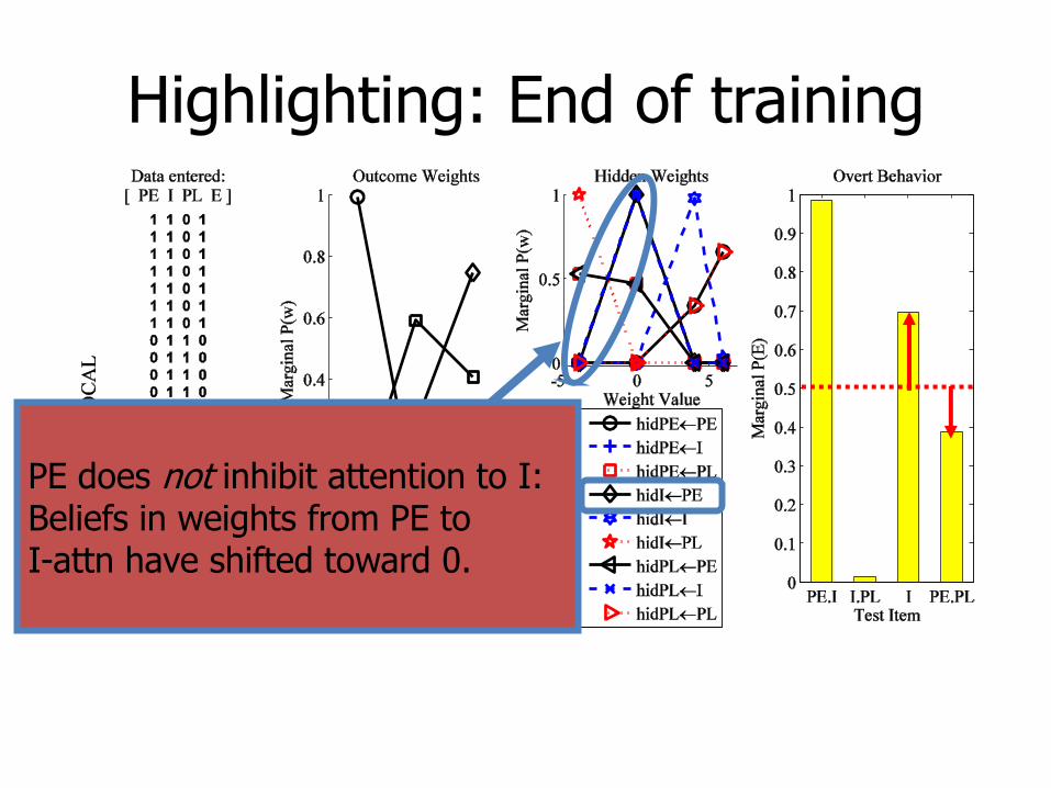
Highlighting: End of training
PE does not inhibit attention to I: Beliefs in weights from PE to I-attn have shifted toward 0.
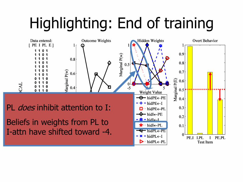
Highlighting: End of training
PL does inhibit attention to I:
Beliefs in weights from PL to I-attn have shifted toward -4.
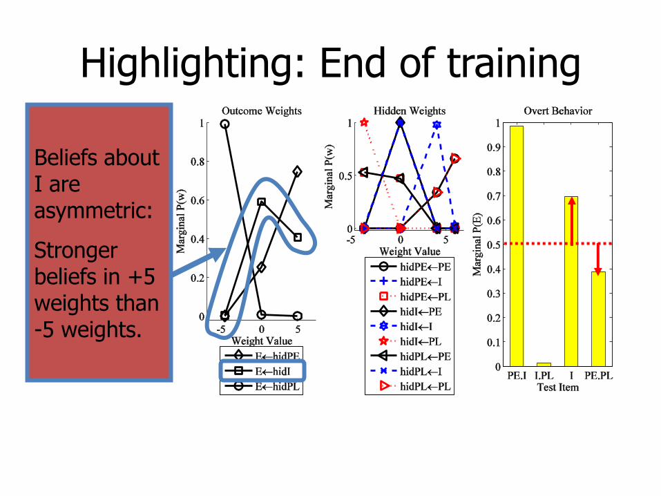
Highlighting: End of training
Beliefs about I are asymmetric:
Stronger beliefs in +5 weights than -5 weights.
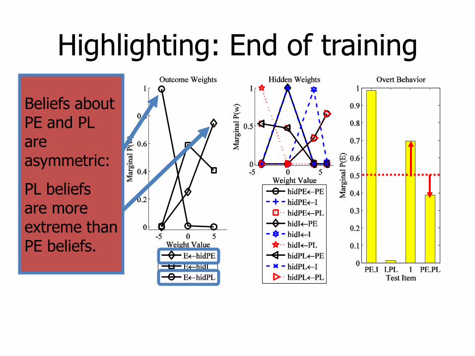
Highlighting: End of training
Beliefs about PE and PL are asymmetric:
PL beliefs are more extreme than PE beliefs.
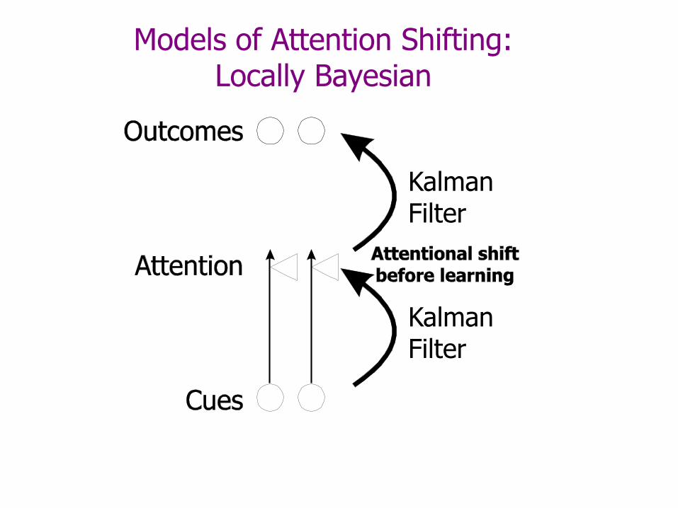
Models of Attention Shifting: Locally Bayesian
Kalman Filter
Kalman Filter
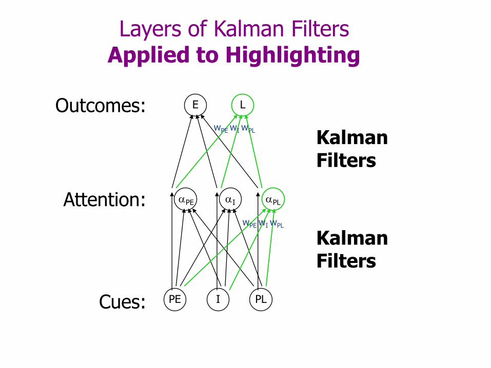
Layers of Kalman Filters Applied to Highlighting
Kalman Filters
Kalman Filters
E
PE I PL
L
wPE wI wPL
I PLPE
wPE wI wPL
Cues:
Attention:
Outcomes:

Layers of Kalman Filters:Likelihood and Prior Distributions
E
PE I PL
L
wPE wI wPL
I PLPE
wPE wI wPL
Cues:
Attention:
Outcomes:
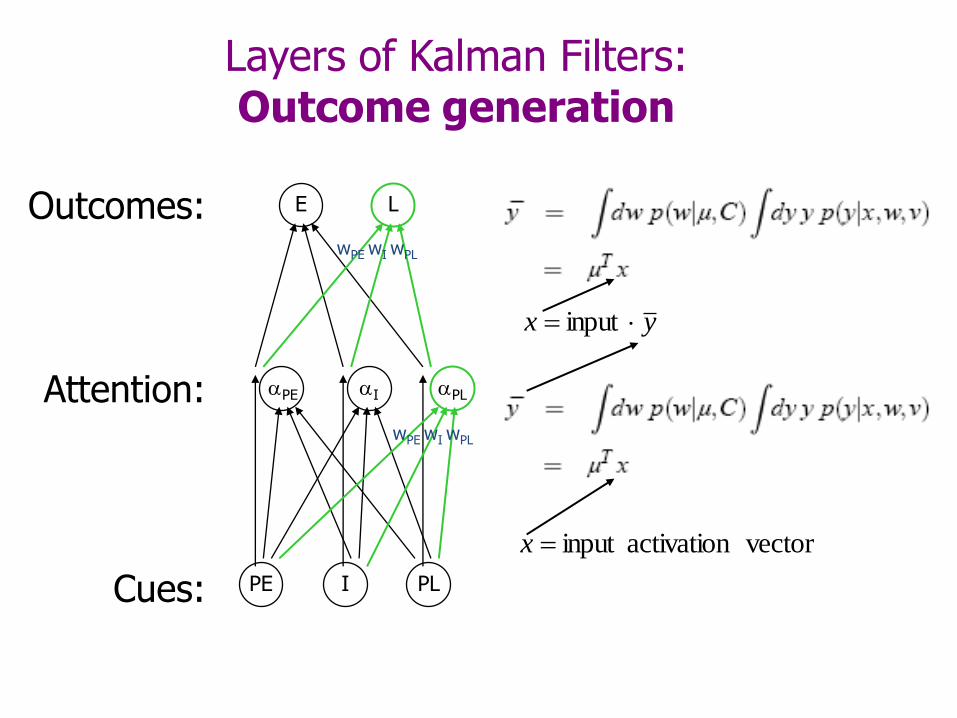
Layers of Kalman Filters:Outcome generation
Cues:
Attention:
Outcomes:
vectoractivationinput x
yx input
E
PE I PL
L
wPE wI wPL
I PLPE
wPE wI wPL
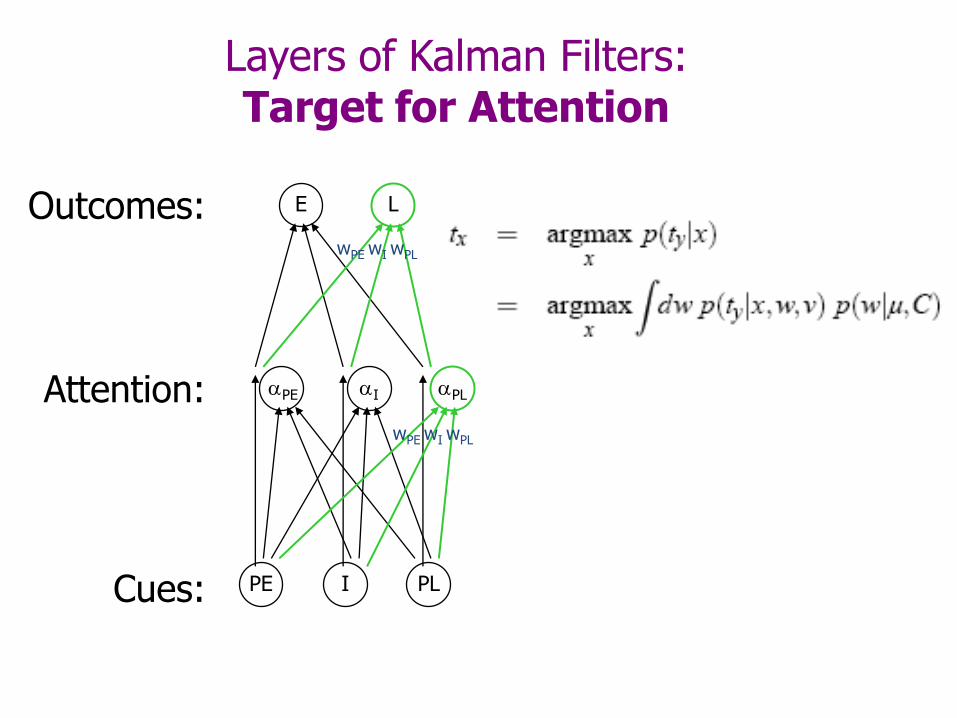
Layers of Kalman Filters:Target for Attention
Cues:
Attention:
Outcomes: E
PE I PL
L
wPE wI wPL
I PLPE
wPE wI wPL
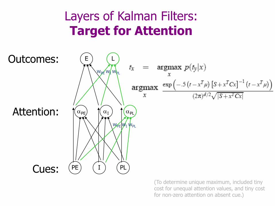
Layers of Kalman Filters:Target for Attention
Cues:
Attention:
Outcomes:
(To determine unique maximum, included tiny cost for unequal attention values, and tiny cost for non-zero attention on absent cue.)
E
PE I PL
L
wPE wI wPL
I PLPE
wPE wI wPL

Layers of Kalman Filters:Dynamics and Bayesian Learning
Cues:
Attention:
Outcomes: E
PE I PL
L
wPE wI wPL
I PLPE
wPE wI wPL
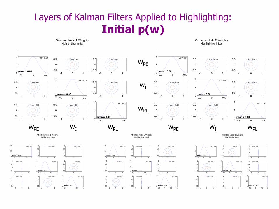
Layers of Kalman Filters Applied to Highlighting:
Initial p(w)Outcome Node 1 Weights
Highlighting Initial
-0.5 0 0.50
1
2var = 0.04
mean = 0.00
cov = 0.00
-1 0 1
-0.5
0
0.5 cov = 0.00
-1 0 1
-0.5
0
0.5
cov = 0.00
-1 0 1
-0.5
0
0.5
-0.5 0 0.50
1
2var = 0.04
mean = 0.00
cov = 0.00
-1 0 1
-0.5
0
0.5
cov = 0.00
-1 0 1
-0.5
0
0.5 cov = 0.00
-1 0 1
-0.5
0
0.5
-0.5 0 0.50
1
2var = 0.04
mean = 0.00
Outcome Node 2 WeightsHighlighting Initial
-0.5 0 0.50
1
2var = 0.04
mean = 0.00
cov = 0.00
-1 0 1
-0.5
0
0.5 cov = 0.00
-1 0 1
-0.5
0
0.5
cov = 0.00
-1 0 1
-0.5
0
0.5
-0.5 0 0.50
1
2var = 0.04
mean = 0.00
cov = 0.00
-1 0 1
-0.5
0
0.5
cov = 0.00
-1 0 1
-0.5
0
0.5 cov = 0.00
-1 0 1
-0.5
0
0.5
-0.5 0 0.50
1
2var = 0.04
mean = 0.00
Attention Node 3 WeightsHighlighting Initial
-0.5 0 0.5 10
1
2var = 0.04
mean = 0.00
cov = 0.00
-1 0 1
-0.5
0
0.5
1 cov = 0.00
0 1 2
-0.5
0
0.5
1
cov = 0.00
-1 0 1
-0.5
0
0.5
1
-0.5 0 0.5 10
1
2var = 0.04
mean = 0.00
cov = 0.00
0 1 2
-0.5
0
0.5
1
cov = 0.00
-1 0 1
-0.5
0
0.5
1 cov = 0.00
-1 0 1
-0.5
0
0.5
1
-0.5 0 0.5 10
20
40var = 0.00
mean = 1.00
Attention Node 2 WeightsHighlighting Initial
-0.5 0 0.5 10
1
2var = 0.04
mean = 0.00
cov = 0.00
0 1 2
-0.5
0
0.5
1 cov = 0.00
-1 0 1
-0.5
0
0.5
1
cov = 0.00
-1 0 1
-0.5
0
0.5
1
-0.5 0 0.5 10
20
40var = 0.00
mean = 1.00
cov = 0.00
-1 0 1
-0.5
0
0.5
1
cov = 0.00
-1 0 1
-0.5
0
0.5
1 cov = 0.00
0 1 2
-0.5
0
0.5
1
-0.5 0 0.5 10
1
2var = 0.04
mean = 0.00
Attention Node 1 WeightsHighlighting Initial
-0.5 0 0.5 10
20
40var = 0.00
mean = 1.00
cov = 0.00
-1 0 1
-0.5
0
0.5
1 cov = 0.00
-1 0 1
-0.5
0
0.5
1
cov = 0.00
0 1 2
-0.5
0
0.5
1
-0.5 0 0.5 10
1
2var = 0.04
mean = 0.00
cov = 0.00
-1 0 1
-0.5
0
0.5
1
cov = 0.00
0 1 2
-0.5
0
0.5
1 cov = 0.00
-1 0 1
-0.5
0
0.5
1
-0.5 0 0.5 10
1
2var = 0.04
mean = 0.00
wPE wI wPL wPE wI wPL
wPL
wI
wPE

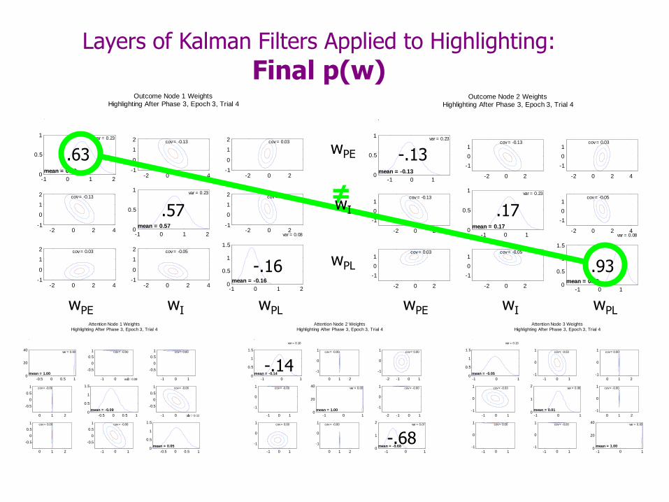
Layers of Kalman Filters Applied to Highlighting:
Final p(w)Outcome Node 1 Weights
Highlighting After Phase 3, Epoch 3, Trial 4
-1 0 1 20
0.5
1var = 0.23
mean = 0.63
cov = -0.13
-2 0 2 4-1
0
1
2 cov = 0.03
-2 0 2-1
0
1
2
cov = -0.13
-2 0 2 4-1
0
1
2
-1 0 1 20
0.5
1var = 0.23
mean = 0.57
cov = -0.05
-2 0 2-1
0
1
2
cov = 0.03
-2 0 2 4-1
0
1
2 cov = -0.05
-2 0 2 4-1
0
1
2
-1 0 1 20
0.5
1
1.5
var = 0.08
mean = -0.16
Outcome Node 2 WeightsHighlighting After Phase 3, Epoch 3, Trial 4
-1 0 10
0.5
1var = 0.23
mean = -0.13
cov = -0.13
-2 0 2
-1
0
1cov = 0.03
-2 0 2 4
-1
0
1
cov = -0.13
-2 0 2
-1
0
1
-1 0 10
0.5
1var = 0.23
mean = 0.17
cov = -0.05
-2 0 2 4
-1
0
1
cov = 0.03
-2 0 2
-1
0
1cov = -0.05
-2 0 2
-1
0
1
-1 0 10
0.5
1
1.5
var = 0.08
mean = 0.93
Attention Node 1 WeightsHighlighting After Phase 3, Epoch 3, Trial 4
-0.5 0 0.5 10
20
40var = 0.00
mean = 1.00
cov = -0.00
-1 0 1
-0.5
0
0.5
1 cov = 0.00
-1 0 1
-0.5
0
0.5
1
cov = -0.00
0 1 2
-0.5
0
0.5
1
-0.5 0 0.5 10
0.5
1
1.5
var = 0.09
mean = -0.09
cov = -0.06
-1 0 1
-0.5
0
0.5
1
cov = 0.00
0 1 2
-0.5
0
0.5
1 cov = -0.06
-1 0 1
-0.5
0
0.5
1
-0.5 0 0.5 10
0.5
1
1.5
var = 0.11
mean = 0.05
Attention Node 2 WeightsHighlighting After Phase 3, Epoch 3, Trial 4
-1 0 10
0.5
1
1.5
var = 0.10
mean = -0.14
cov = -0.00
0 1 2
-1
0
1 cov = 0.00
-2 -1 0 1
-1
0
1
cov = -0.00
-1 0 1
-1
0
1
-1 0 10
20
40var = 0.00
mean = 1.00
cov = -0.00
-2 -1 0 1
-1
0
1
cov = 0.00
-1 0 1
-1
0
1 cov = -0.00
0 1 2
-1
0
1
-1 0 10
1
2var = 0.07
mean = -0.68
Attention Node 3 WeightsHighlighting After Phase 3, Epoch 3, Trial 4
-1 0 10
0.5
1
1.5
var = 0.13
mean = -0.05
cov = -0.03
-1 0 1
-1
0
1 cov = 0.00
0 1 2
-1
0
1
cov = -0.03
-1 0 1
-1
0
1
-1 0 10
1
2var = 0.06
mean = 0.01
cov = -0.00
0 1 2
-1
0
1
cov = 0.00
-1 0 1
-1
0
1 cov = -0.00
-1 0 1
-1
0
1
-1 0 10
20
40var = 0.00
mean = 1.00
.63
.57
-.16
-.13
.17
.93
-.14
-.68
wPE wI wPL wPE wI wPL
wPL
wI
wPE
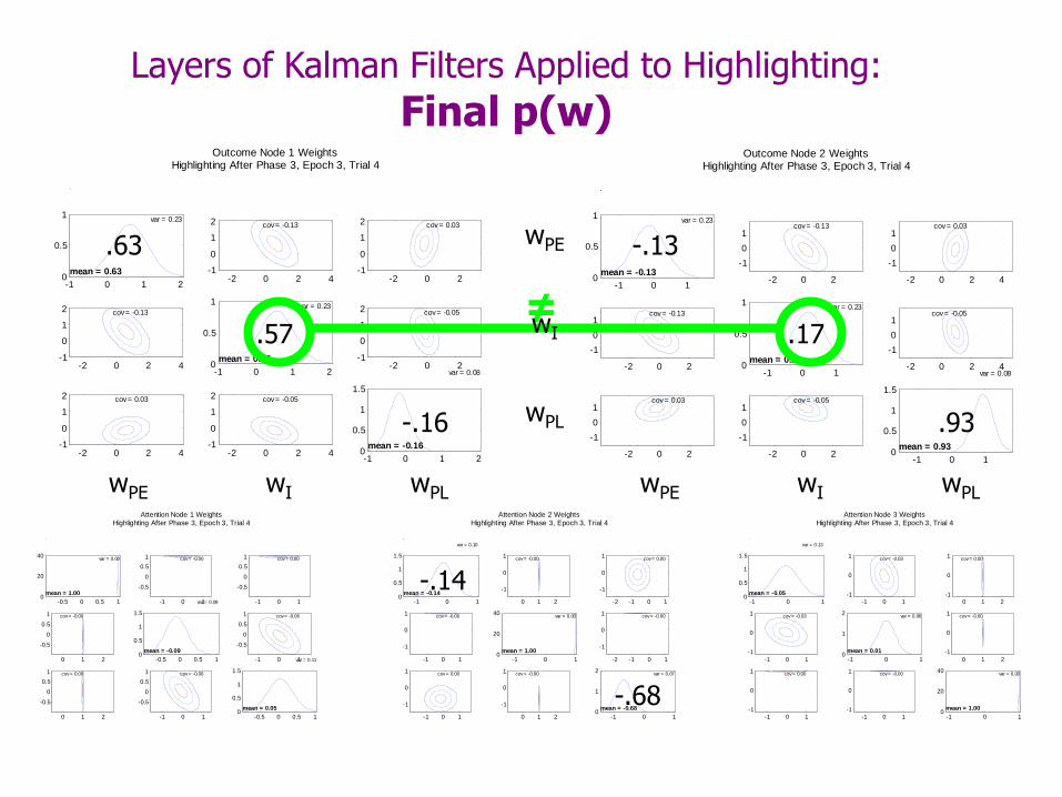
Layers of Kalman Filters Applied to Highlighting:
Final p(w)Outcome Node 1 Weights
Highlighting After Phase 3, Epoch 3, Trial 4
-1 0 1 20
0.5
1var = 0.23
mean = 0.63
cov = -0.13
-2 0 2 4-1
0
1
2 cov = 0.03
-2 0 2-1
0
1
2
cov = -0.13
-2 0 2 4-1
0
1
2
-1 0 1 20
0.5
1var = 0.23
mean = 0.57
cov = -0.05
-2 0 2-1
0
1
2
cov = 0.03
-2 0 2 4-1
0
1
2 cov = -0.05
-2 0 2 4-1
0
1
2
-1 0 1 20
0.5
1
1.5
var = 0.08
mean = -0.16
Outcome Node 2 WeightsHighlighting After Phase 3, Epoch 3, Trial 4
-1 0 10
0.5
1var = 0.23
mean = -0.13
cov = -0.13
-2 0 2
-1
0
1cov = 0.03
-2 0 2 4
-1
0
1
cov = -0.13
-2 0 2
-1
0
1
-1 0 10
0.5
1var = 0.23
mean = 0.17
cov = -0.05
-2 0 2 4
-1
0
1
cov = 0.03
-2 0 2
-1
0
1cov = -0.05
-2 0 2
-1
0
1
-1 0 10
0.5
1
1.5
var = 0.08
mean = 0.93
Attention Node 1 WeightsHighlighting After Phase 3, Epoch 3, Trial 4
-0.5 0 0.5 10
20
40var = 0.00
mean = 1.00
cov = -0.00
-1 0 1
-0.5
0
0.5
1 cov = 0.00
-1 0 1
-0.5
0
0.5
1
cov = -0.00
0 1 2
-0.5
0
0.5
1
-0.5 0 0.5 10
0.5
1
1.5
var = 0.09
mean = -0.09
cov = -0.06
-1 0 1
-0.5
0
0.5
1
cov = 0.00
0 1 2
-0.5
0
0.5
1 cov = -0.06
-1 0 1
-0.5
0
0.5
1
-0.5 0 0.5 10
0.5
1
1.5
var = 0.11
mean = 0.05
Attention Node 2 WeightsHighlighting After Phase 3, Epoch 3, Trial 4
-1 0 10
0.5
1
1.5
var = 0.10
mean = -0.14
cov = -0.00
0 1 2
-1
0
1 cov = 0.00
-2 -1 0 1
-1
0
1
cov = -0.00
-1 0 1
-1
0
1
-1 0 10
20
40var = 0.00
mean = 1.00
cov = -0.00
-2 -1 0 1
-1
0
1
cov = 0.00
-1 0 1
-1
0
1 cov = -0.00
0 1 2
-1
0
1
-1 0 10
1
2var = 0.07
mean = -0.68
Attention Node 3 WeightsHighlighting After Phase 3, Epoch 3, Trial 4
-1 0 10
0.5
1
1.5
var = 0.13
mean = -0.05
cov = -0.03
-1 0 1
-1
0
1 cov = 0.00
0 1 2
-1
0
1
cov = -0.03
-1 0 1
-1
0
1
-1 0 10
1
2var = 0.06
mean = 0.01
cov = -0.00
0 1 2
-1
0
1
cov = 0.00
-1 0 1
-1
0
1 cov = -0.00
-1 0 1
-1
0
1
-1 0 10
20
40var = 0.00
mean = 1.00
.63
.57
-.16
-.13
.17
.93
-.14
-.68
≠
wPE wI wPL wPE wI wPL
wPL
wI
wPE
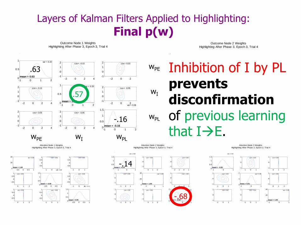
Layers of Kalman Filters Applied to Highlighting:
Final p(w)Outcome Node 1 Weights
Highlighting After Phase 3, Epoch 3, Trial 4
-1 0 1 20
0.5
1var = 0.23
mean = 0.63
cov = -0.13
-2 0 2 4-1
0
1
2 cov = 0.03
-2 0 2-1
0
1
2
cov = -0.13
-2 0 2 4-1
0
1
2
-1 0 1 20
0.5
1var = 0.23
mean = 0.57
cov = -0.05
-2 0 2-1
0
1
2
cov = 0.03
-2 0 2 4-1
0
1
2 cov = -0.05
-2 0 2 4-1
0
1
2
-1 0 1 20
0.5
1
1.5
var = 0.08
mean = -0.16
Outcome Node 2 WeightsHighlighting After Phase 3, Epoch 3, Trial 4
-1 0 10
0.5
1var = 0.23
mean = -0.13
cov = -0.13
-2 0 2
-1
0
1cov = 0.03
-2 0 2 4
-1
0
1
cov = -0.13
-2 0 2
-1
0
1
-1 0 10
0.5
1var = 0.23
mean = 0.17
cov = -0.05
-2 0 2 4
-1
0
1
cov = 0.03
-2 0 2
-1
0
1cov = -0.05
-2 0 2
-1
0
1
-1 0 10
0.5
1
1.5
var = 0.08
mean = 0.93
Attention Node 1 WeightsHighlighting After Phase 3, Epoch 3, Trial 4
-0.5 0 0.5 10
20
40var = 0.00
mean = 1.00
cov = -0.00
-1 0 1
-0.5
0
0.5
1 cov = 0.00
-1 0 1
-0.5
0
0.5
1
cov = -0.00
0 1 2
-0.5
0
0.5
1
-0.5 0 0.5 10
0.5
1
1.5
var = 0.09
mean = -0.09
cov = -0.06
-1 0 1
-0.5
0
0.5
1
cov = 0.00
0 1 2
-0.5
0
0.5
1 cov = -0.06
-1 0 1
-0.5
0
0.5
1
-0.5 0 0.5 10
0.5
1
1.5
var = 0.11
mean = 0.05
Attention Node 2 WeightsHighlighting After Phase 3, Epoch 3, Trial 4
-1 0 10
0.5
1
1.5
var = 0.10
mean = -0.14
cov = -0.00
0 1 2
-1
0
1 cov = 0.00
-2 -1 0 1
-1
0
1
cov = -0.00
-1 0 1
-1
0
1
-1 0 10
20
40var = 0.00
mean = 1.00
cov = -0.00
-2 -1 0 1
-1
0
1
cov = 0.00
-1 0 1
-1
0
1 cov = -0.00
0 1 2
-1
0
1
-1 0 10
1
2var = 0.07
mean = -0.68
Attention Node 3 WeightsHighlighting After Phase 3, Epoch 3, Trial 4
-1 0 10
0.5
1
1.5
var = 0.13
mean = -0.05
cov = -0.03
-1 0 1
-1
0
1 cov = 0.00
0 1 2
-1
0
1
cov = -0.03
-1 0 1
-1
0
1
-1 0 10
1
2var = 0.06
mean = 0.01
cov = -0.00
0 1 2
-1
0
1
cov = 0.00
-1 0 1
-1
0
1 cov = -0.00
-1 0 1
-1
0
1
-1 0 10
20
40var = 0.00
mean = 1.00
.63
.57
-.16
-.13
.17
.93
-.14
-.68
wPE wI wPL wPE wI wPL
wPL
wI
wPE Inhibition of I by PL prevents disconfirmation of previous learning that IE.
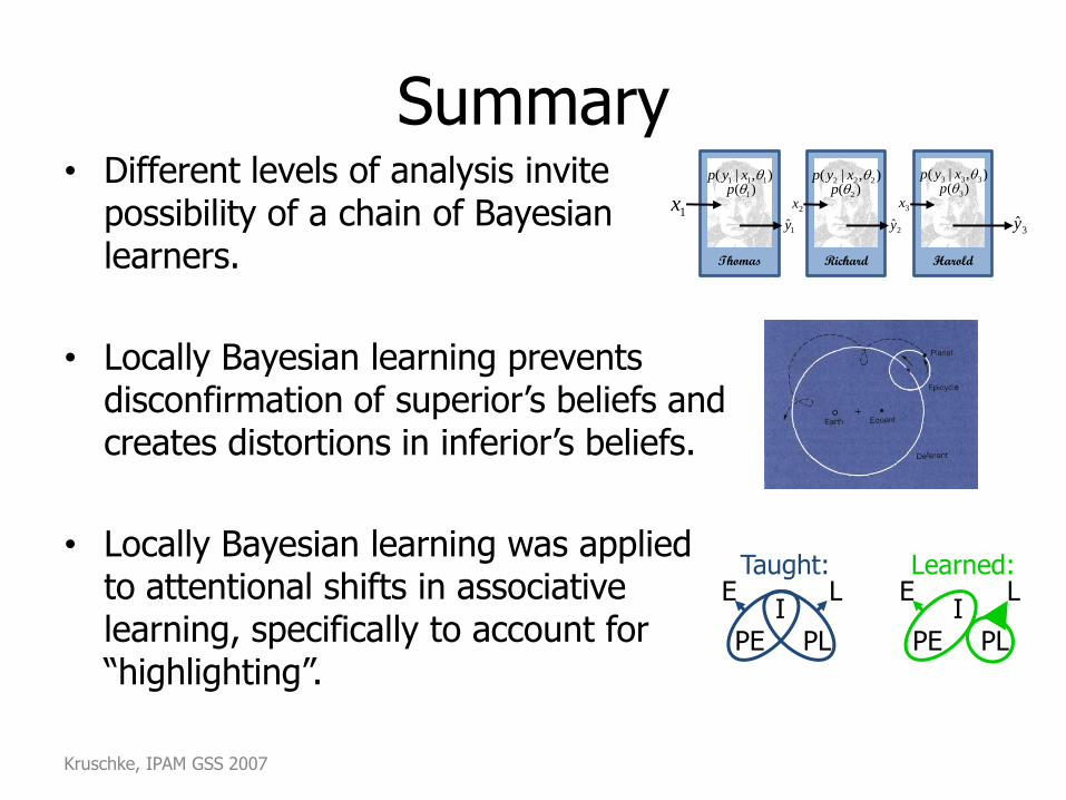
Summary
• Locally Bayesian learning was applied to attentional shifts in associative learning, specifically to account for “highlighting”.
Kruschke, IPAM GSS 2007
IPE PL
E LTaught:
IPE PL
E LLearned:
),|( 111 xyp)( 1p
1x3y
Thomas Richard Harold
),|( 222 xyp ),|( 333 xyp)( 2p )( 3p
1y 2y
2x 3x
• Different levels of analysis invite possibility of a chain of Bayesian learners.
• Locally Bayesian learning prevents disconfirmation of superior’s beliefs and creates distortions in inferior’s beliefs.

Future Directions
• Better models and priors for application to associative learning, to expand scope and quantitatively fit human learning.
• Applications to other domains and phenomena. (Please suggest!)
• Formal analysis of global behavior of system of Bayesian agents.
Kruschke, IPAM GSS 2007