Inequality and Genes (and FamilyBackground)

Markus Jäntti

Swedish Institute for Social ResearchStockholm University

1 februari 2018

Introduction

I intergenerational associations and the importance of familybackground in economic outcomes

I ”genes”:I genome-wide association studies (”GWAS”)I population genetic models

I (economic) outcomes:I abilities (cognitive, socio-emotional [”non-cognitive”])I income (disposable family income, earnings, . . . )I education

I inequality: the distribution of economic outcomes

Intergenerational economic associationsI suppose yO and yP are the “permanent income” of a pair of

offspring and parentI the intergenerational income elasticity is the measure for

which most evidence is available:

yO = α+ βyP + ε (1)

I two interpretations for β:I the slope of the conditional expectation of offspring income,

given parental income (“mechanical”):

β :=∂E[yO |yP ]

∂yP(2)

I the causal effect of a change in parental income on childincome (“economic”):

β :=∂y∗O∂yP

(3)

the y∗O conveys that offspring income is at least in part theresult of optimizing behavior on the part of parents

The causal interpretation

I the Becker och Tomes (1979, 1986) model of parentalinvestment in child human capital inspirs much empiricalwork

I a simplified version is due to Solon (2004), with offspringincome depending on parental income by

yi,O = µ∗ + [(1− γ)θp]yi,P + pei,o. (4)

I p is the return on human capitalI e is offspring human capital endowmentI γ measures the progressivity in human capitalI θ measures how effectively human capital investments turn

into capitalI λ captures the IG transmission of the ability (such as

genetic transmission)

The causal interpretation

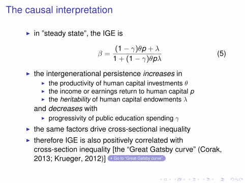
I in ”steady state”, the IGE is

β =(1− γ)θp + λ

1 + (1− γ)θpλ(5)

I the intergenerational persistence increases inI the productivity of human capital investments θI the income or earnings return to human capital pI the heritability of human capital endowments λ

and decreases withI progressivity of public education spending γ

I the same factors drive cross-sectional inequalityI therefore IGE is also positively correlated with

cross-section inequality [the “Great Gatsby curve” (Corak,2013; Krueger, 2012)] Go to “Great Gatsby curve”

Cross-national results

I IGEs: 0.15-0.50 (acc. to Corak’s (2013) version of theGreat Gatsby Curve)

I IGCs: possibly less variation (Corak, Lindquist ochBhaskar Mazumder, 2013) but there is less comparableinformation about IGCs.

I Thus: R-squares (IGC2) from 0.02-0.25.

Sibling correlationI The prototypical model:

Yij = ai + bij , a ⊥ b (6)

I the “family effect” a shared by sibling in family i , variance σ2a

I the “individual effect” b unique to individual j in family i(orthogonal to a), variance σ2

b

I the population variance of the outcome Y is

σ2 = σ2a + σ2

b, (7)

I the share of variance attributable to family background (its“R2”) is

ρ =σ2

a

σ2a + σ2

b(8)

which coincides with the Pearson correlation for siblingpairs

A sibling correlation captures more than anintergenerational correlation (IGC)

I an omnibus measure – captures both observed andunobserved family background (and neighborhood) factors

I yet it is a lower bound, because siblings don’t shareeverything from the family background

I moreover,sibling correlation = IGC2 + other shared factors that areuncorrelated with parental Y

Brother correlations in earnings and income

Country Estimate SourceDenmark 0.20 Schnitzlein (2013)China 0.57 Eriksson och Zhang (2012)Finland 0.26 Österbacka (2001)Germany 0.43 Schnitzlein (2013)Norway 0.14 Björklund, Eriksson m. fl. (2002)Sweden 0.32 Björklund, Jäntti och Lindquist (2009)USA 0.49 Bhashkar Mazumder (2008)

Sibling correlations in years of schooling

Country Sibling type Estimate SourceGermany Brothers .66 Schnitzlein (2013)Germany Sisters .55 Schnitzlein (2013)Norway Mixed sexes .41 Björklund och Salvanes (2011)Sweden Brothers .43 Björklund och Jäntti (2012)Sweden Sisters .40 Björklund och Jäntti (2012)USA Mixed sexes .60 Bhashkar Mazumder (2008)

These quite high numbers are only lower bounds.What is missing?

1. differential treatment by parents. Will not be captured if itcreates differences, but is part of family background.

2. full siblings have only about half of (initial) genes incommon. But each individual has 100% of her (initial)genes from the parents.

3. not all environmental experience and “shocks” are shared,only some. Thus some environmental stuff is missing.

Sibling correlations vs. intergenerational correlations,Swedish estimates

I recall that:sibling correlation = IGC2 + other shared factors that areuncorrelated with parental Y

ρ IGC2 = R2 Other factorsBrothers:Earnings .24 .02 .22Schooling .46 .15 .31Sisters:Schooling .40 .11 .29

Genetics and inequalitySee Beauchamp m. fl. (2011) och Manski (2011)

Two types of approaches:I modern: genome-wide association studies and inequalityI traditional: population-genetic modelling

Genome-wide association studies and inequalitySee e.g. Beauchamp m. fl. (2011) och Chabris m. fl. (2012)

I linking genetic markers/single nucleotide polymorphisms(SNPs) to specific (economic) traits

I a quickly moving and expanding field of study . . .I . . . that yields both many insights but also many

disappointments . . .I . . . but one which as of yet has yielded very few insights

into the genetic basis of economic inequality

GWAS is providing information from the research frontier, butnow mostly providing insights into the associations with thelevels of economic traits rather than with the inequality ofeconomic outcomes.

Cautionary noteFrom ”Most Reported Genetic Associations With General Intelligence Are ProbablyFalse Positives”, (Chabris m. fl., 2012)

General intelligence (g) and virtually all other behavioral traits areheritable. Associations between g and specific single-nucleotidepolymorphisms (SNPs) in several candidate genes involved in brainfunction have been reported. We sought to replicate publishedassociations between g and 12 specific genetic variants [. . . ] usingdata sets from three independent, well-characterized longitudinalstudies with samples of 5,571, 1,759, and 2,441 individuals. Of 32independent tests across all three data sets, only 1 was nominallysignificant. By contrast, power analyses showed that we should haveexpected 10 to 15 significant associations, given reasonableassumptions for genotype effect sizes. [. . . ] We conclude that themolecular genetics of psychology and social science requiresapproaches that go beyond the examination of candidate genes.

Population genetic models [PGM] and inequalityI started long before the role of molecular genetics was well

understoodI relies (often) on studies of twins (MZ/DZ, reared

together/apart) but can rely on general kinshipI an important aim has been to estimate the extent to which

variation in some trait (IQ; personality measures;education; income) is genetic (heritability)

I relies on

outcome = genetic factors + environmental factors (9)

orY = G + E

I ”environmental factors” E are further separated into”shared” ones (S; such as the behaviour of parents towardtheir children) and non-shared ones (U)

Illustrative example: PGM for earnings in SwedenBjörklund, Jäntti och Solon (2005)

I strategy: estimate highly restricted, unrealistically simplemodel and extend it gradually (ad hoc)

I simple model of earnings determination:

Y = gG + sS + uU (10)

I Y is permanent (=long-run) earnings. Normalize thevariance of Y to unity.

I G, S and U are additive gene effect, shared andnon-shared environment that are unobserved, latentvariables. Normalized to have unit variance and zero mean.

I g, s and u are “factor loadings”, parameters to beestimated. Interest in g2 (”heritability”) and s2 in particular.

I by assumption, the population variance in Y is

Var(Y ) ≡ 1 = g2 + s2 + u2. (11)

I the parameters g2 and s2 can be identified by correlationsin Y between relatives.

I let Y and Y ′ be two related persons:

Cov(Y ,Y ′) = g2Cov(G,G′) + s2Cov(S,S′) + u2Cov(S,S′)+2gbCov(G,S′) + 2guCov(G,U ′) + 2suCov(S,U ′).

(12)

I in order to estimate these parameters, we must place anumber of restrictions on the covariances of the latentvariable.

I assume non-shared environment U un-correlated witheverything

Cov(G,U ′) = Cov(S,U ′) = Cov(U,U ′) = 0 (13)

I if mating is random, there are no dominant gene effectsnor non-additive gene effects, Cov(G,G′) is 1, .5 and .25for identical twins, fraternal twins as well as full siblings andhalf siblings

I for siblings reared together, Cov(S,S′) is 1, 0 otherwiseI focus here on brother only (the paper reports results for

both brothers and sisters)

”Design matrix” for estimating variance componentsfrom sibling correlations

Sibling type Rearing Cov(G,G′) Cov(S,S′)Model 1

MZ twins Together 1 1DZ twins Together 0.5 1MZ twins Apart 1 0DZ twins Apart 0.5 0Full sibs Together 0.5 1Half sibs Together 0.25 1Full sibs Apart 0.5 0Half sibs Apart 0.25 0Adopted Together 0 1

Three variations to the simple model (1→ 2{A,B,C})

A Gene-envcorrelation

I replace theassumption thatCov(G,S′) = 0 withparameters to beestimated

I one for biologicalsiblings rearedtogether, one forthose reared apart,one for adoptivesiblings

B Gene-genecorrelation

I suppose that someof the restrictiveassumptions thatgenerateCov(G,G′) of 1, .5,.25 are violated

I allow correlationsbe different foridentical twins,fraternal twins, halfsiblings andadoptive siblings

C Sharedenvironment

I suppose “rearing”,or the sharedenvironment is noton, off

I normalizeCov(S,S′) for MZtwins rearedtogether, one forfraternal twinstogether, one forother siblingsreared together andone for siblingsreared apart

Consequences of changes to assumptions forMZ/together genetic/environment components

”Raw” Genetic Environmentalcorrelation component component

Model 1 .363 .281 .0382A Vary G,S .363 .250-.314 .020-.0842B Vary G,G′ .363 .320 .0372C More env sim for MZ .363 .199 .164

Additional remarks

I in utero shocks are now known to be important . . .I . . . but the PGM assigns all pre-birth factors to genesI PGM models tend to normalize the variances and work

only with correlations . . .I . . . which, by construction, abstracts from distributional

dynamicsI however, population genetic analysis of family associations

provides useful insights and structure to understandingfamily associations in outcomes

See, e.g., Kamin och Goldberger (2002), Feldman, Otto ochChristiansen (1999).

Policy implications of PGMSee Goldberger (1979) och Manski (2011)

I near-sightedness (aka. myopia)

I it seems reasonable to suppose that myopia is highly heritable

I does it follow that there is no appropriate policy response to it?

I no; distributing eyeglasses to the myopic is an effective way toalleviate nearsightedness

I the fact of high heritablility tells us little or nothing of howamenable a disadvantage is to interventions

I for that, we need estimates of the causal effect of interventions

”The conclusion is that the heredity-IQ controversy has been a ’talefull of sound and fury, signifying nothing’. To suppose that one canestablish effects of an intervention process when it does not occur inthe data is plainly ludicrous.” [Kempthorne, 1978, cited by Manski(2011))]

Concluding remarks

I population and molecular genetics will be continued to beexplored by social scientists . . .

I . . . and the latter are likely to increasingly provide insightsinto the scope for policy interventions to be effective

I the dynamics of economic inequality, the extent to whichthere is equality of opportunity, continue to be of greatinterest

I many interesting issues to be studies apart from the role ofgenetics in these processes

I e.g., what are the things that families do that is not capturedin direct IG transmission?

I can and do policy interventions alter the strength of familyassociations?

Trends in income inequality

Policy interventions and family associations

I public expenditures in US affects IGE (Mayer och Lopoo,2008)

I comprehensive school reform in Sweden, Finland hadsizeable impact on IGE

Comprehensive school reform in Finland

I Comprehensive school thus:I moved tracking from age 11 to age 16I increased length of compulsory schooling by one yearI led to integration of students in same schools between

ages 11-16I made all follow same curriculum between ages 11-16

(although some variation initially)I The reform was implemented in 5 stages between 1972

and 1977, affecting cohorts born 1961-1965, starting in thenorth and ending in the capital area.

I We use the stage-wise implementation to estimate theeffect of the reform by comparing the correlation amongpairs of brothers who either were or were not affected bycomprehensive school

The impact of comprehensive school reform in Finland

Father’s earnings 0.277 0.297 0.298(0.014) (0.011) (0.010)

Father’s earnings×Reform -0.055 -0.069(0.009) (0.022)

Reform -0.065 -0.019(0.012) (0.021)

Source: Pekkarinen, Uusitalo och Kerr (2009)

Inequality is on the increaseAverage annual growth across the income distribution ca 1985-2008 (before the GreatRecession) [Source: OECD (2011)]

%-changeOverall Bottom 10% Top 10 %

Australia 3.6 3.0 4.5Austria 1.3 0.6 1.1Canada 1.1 0.9 1.6Denmark 1.0 0.7 1.5Finland 1.7 1.2 2.5France 1.2 1.6 1.3Germany 0.9 0.1 1.6Italy 0.8 0.2 1.1Mexico 1.4 0.8 1.7Netherlands 1.4 0.5 1.6Norway 2.3 1.4 2.7Portugal 2.0 3.6 1.1Spain 3.1 3.9 2.5Sweden 1.8 0.4 2.4United Kingdom 2.1 0.9 2.5United States 1.3 0.5 1.9OECD27 1.7 1.3 1.9

What if the Great Gatsby curve persists whileinequality increases?

I the “Great Gatsby” curve plots the intergenerationalpersistence of income against income inequality in(roughly) the parental generation

I income inequality has increasedI what can be expected of persistence?I caveat: this is highly speculative and is intended as food

for thought

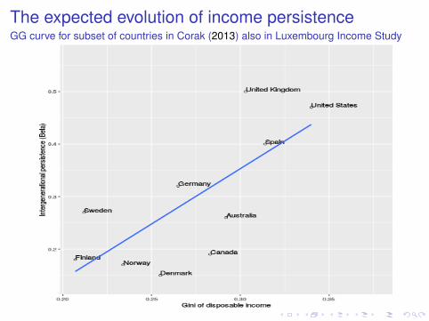
The expected evolution of income persistenceGG curve for subset of countries in Corak (2013) also in Luxembourg Income Study

The expected evolution of income persistenceGG curve for subset of countries in Corak (2013) also in Luxembourg Income Study

The expected evolution of income persistenceGG curve for subset of countries in Corak (2013) also in Luxembourg Income Study

The expected evolution of income persistenceGG curve for subset of countries in Corak (2013) also in Luxembourg Income Study

The Great Gatsby curvethe relationship between intergenerational earnings persistence and cross-sectionalincome inequality; Source: Corak (2013, Figure 1). Go back to Causal intrepretation