inferring planetary obliquity using rotational &...

Mon. Not. R. Astron. Soc. 000, 1–12 (2015) Printed 16 November 2015 (MN LATEX style file v2.2)

Inferring Planetary Obliquity Using Rotational & OrbitalPhotometry

J. C. Schwartz1,2,3?†, C. Sekowski4,5, H. M. Haggard4, E. Palle6, and N. B. Cowan2,3†1Department of Physics & Astronomy, Northwestern University, 2145 Sheridan Road, Evanston, IL, 60208, USA2Department Earth & Planetary Sciences, McGill University, 3450 rue University, Montreal, QC, H3A 0E8, CAN3Department of Physics, McGill University, 3600 rue University, Montreal, QC, H3A 2T8, CAN4Physics Program, Bard College, PO Box 5000, Annandale, NY, 12504, USA5Department of Physics, Boston University, 590 Commonwealth Ave, Boston, MA, 02215, USA6Instituto de Astrofıscia de Canarias, Via Lactea s/n, La Laguna, Santa Cruz de Tenerife, 35205, ESP

Submitted to MNRAS

ABSTRACTThe obliquity of a terrestrial planet is an important clue about its formation and critical to itsclimate. Previous studies using simulated photometry of Earth show that continuous observa-tions over most of a planet’s orbit can be inverted to infer obliquity. We extend this approachto single-epoch observations for planets with arbitrary albedo maps. For diffuse reflection,the flux seen by a distant observer is the product of the planet’s albedo map, the host star’sillumination, and the observer’s visibility of different planet regions. It is useful to treat theproduct of illumination and visibility as the kernel of a convolution; this kernel is unimodaland symmetric. For planets with unknown obliquity, the kernel is not known a priori, but couldbe inferred by fitting a rotational light curve. We analyze this kernel under different viewinggeometries, finding it well described by its longitudinal width and latitudinal position. We useMonte Carlo simulation to estimate uncertainties on these kernel characteristics from varia-tions in a planet’s apparent albedo. We demonstrate that the kernel properties are functions ofobliquity and axial orientation, which may both be inferred even if planets are A) East-Westuniform or spinning rapidly, or B) North-South uniform. We consider degeneracies in theseinferences with a case study, and describe how to tell prograde from retrograde rotation forinclined, oblique planets. This approach could be used to estimate obliquities of terrestrialplanets with modest time investment from flagship direct-imaging missions.

Key words: methods: analytical – planets and satellites: fundamental parameters – methods:statistical.

1 INTRODUCTION

The obliquity of a terrestrial planet encodes information about dif-ferent processes. First, a planet’s axial alignment and spin rate in-form its formation scenario. Numerical simulations have shownthat the spin rates of Earth and Mars are likely caused by a few plan-etesimal impacts (Dones & Tremaine 1993), while perfect accre-tion produces an obliquity distribution that is isotropic (e.g. Kokubo& Ida 2007; Miguel & Brunini 2010). Conversely, Schlichting &Sari (2007) describe how prograde rotation is preferred to retro-grade for a formation model with semi-collisional accretion.

Second, obliquity is important in controlling planetary cli-mate. This has been studied in-depth for Earth under many con-ditions (e.g. Laskar et al. 2004; Pierrehumbert 2010), and high ax-ial tilts can make planets at large semi-major axes more habitable

? E-mail: [email protected]† McGill Space Institute (McGill U.); Institute for Research on Exoplanets(UdeM)

(Williams & Kasting 1997). Furthermore, while the Earth’s spinaxis is stabilized by the Moon (Laskar et al. 1993), obliquities ofseveral Solar System bodies evolve chaotically (Laskar 1994). Thisinfluences searches for hospitable planets, as Spiegel et al. (2009)note that the habitability of terrestrial worlds may depend sensi-tively on how stable the climate is in the short-term.

A planet’s average insolation is set by stellar luminosity andsemi-major axis; insolation at different latitudes is determinedby obliquity and (for eccentric orbits) the axial orientation. Non-oblique planets have a warmer equator and colder poles which donot vary much throughout the year. Modest obliquities produce sea-sons at mid-latitudes because the sub-stellar point moves North andSouth during the orbit (Pierrehumbert 2010). Planets tilted > 54

receive more overall radiation near their poles and have large or-bital variations in temperature (Williams & Pollard 2003). Thus,even limited knowledge of a planet’s obliquity can help constrainthe spatial dependence of insolation and temperature.

Reflected light from terrestrial exoplanets will be studiedwith forthcoming optical and near-infrared space missions, such

c© 2015 RAS

2 J. C. Schwartz et al.

30 60 90 120 150

Orbital Phase

0.1

0.2

0.3

0.4

0.5

0.6

Appare

nt

Alb

edo

0 2 4 6 8

Relative Orbital Phase

0.1

0.2

0.3

0.4

0.5

0.6

Rela

tive A

ppare

nt

Alb

edo

Figure 1. The left panel shows apparent albedo as a function of orbital phase for an arbitrary planet with North-South and East-West albedo markings, seenedge-on with zero obliquity (black) or 45 obliquity (green). The average albedo of the green planet increases during the orbit because brighter latitudesbecome visible and illuminated; this does not happen for the black planet. The vertical bands are each roughly two planetary days, enlarged at right, wherelighter shades represent the fuller phase. For clarity, the rotational curves are shifted and the zero obliquity planet is denoted by a dashed line. The apparentalbedo of either planet varies more over a day when a narrower range of longitudes and albedo markings are visible and illuminated, and vice versa. Orbitaland/or rotational changes in apparent albedo can help one infer a planet’s obliquity.

as ATLAST/HDST (Kouveliotou et al. 2014) and LUVOIR (Post-man et al. 2009). Time-resolved measurements of a rotating planetin one photometric band can reveal its rotation rate (Ford et al.2001; Palle et al. 2008; Oakley & Cash 2009); this helps deter-mine Coriolis forces and predict large-scale circulation. Multi-bandphotometry can reveal colors of clouds and surface features (Fordet al. 2001; Fujii et al. 2010, 2011; Cowan & Strait 2013), and en-ables a longitudinal albedo map to be inferred from disk-integratedlight (Cowan et al. 2009). High-cadence, reflected light measure-ments spanning a full planetary orbit constrain a planet’s obliquityand two-dimensional albedo map (Kawahara & Fujii 2010, 2011;Fujii & Kawahara 2012). This is appropriate for planets that or-bit quickly, but full retrievals grow infeasible as orbital periods in-crease.

Other methods have been proposed for measuring plane-tary obliquities. Seager & Hui (2002) and Barnes & Fortney(2003) demonstrated constraints on oblateness and obliquity us-ing ingress/egress differences in transit light curves; Carter &Winn (2010) extended and applied these techniques to observa-tions of HD 189733b. Kawahara (2012) derived constraints onobliquity from modulation of a planet’s radial velocity during or-bit, while Nikolov & Sainsbury-Martinez (2015) examined theRossiter-McLauglin effect at secondary eclipse for transiting ex-oplanets. One could also measure obliquity with infrared wave-lengths, using polarized rotational light curves (De Kok et al. 2011)and orbital variations (e.g. Gaidos & Williams 2004; Cowan et al.2013). We look to constrain a planet’s spin axis with diffuse re-flected light photometry—an extension of Kawahara & Fujii (2010,2011) and Fujii & Kawahara (2012) to observations at only one ortwo orbital phases.

Light curves of planets encode the viewing geometry andhence a planet’s obliquity because different latitudes are impingedby starlight at different orbital phases. To see this, consider a planetwith no obliquity in an edge-on, circular orbit. The star always il-luminates the Northern and Southern hemispheres equally, and wenever view some latitudes more than others. If instead this planetwere tilted, the Northern hemisphere would be lit first, then theSouthern hemisphere half an orbit later. If the planet’s Northern

and Southern hemispheres have different albedo markings, its ap-parent albedo (Qui et al. 2003; Cowan et al. 2009) would changeduring its orbit (left panel of Figure 1) and these changes can helpone constrain the obliquity.

We may also learn about a planet’s obliquity as it rotates.Imagine a zero obliquity planet in a face-on, circular orbit: the ob-server always sees the Northern pole with half the longitudes illu-minated. For an oblique planet, however, more longitudes would belit when the visible pole leans towards the star, and vice versa. Zeroobliquity planets in edge-on orbits are similar, since more longi-tudes are lit near superior conjunction, or fullest phase. If the planethas East-West albedo variations, then this longitudinal width willmodulate the apparent albedo of the planet as it spins (right panelof Figure 1), which again helps one constrain the obliquity.

Our work is organized as follows: in Section 2 we summarizethe observer viewing geometry and explain the reflective kernel,both in two- and one-dimensional forms. Section 3.1 introduces acase study planet and describes the kernel at single orbital phases;we consider time evolution in Section 3.2. We discuss our assump-tions about determining the kernel in Section 4.1, then develop ourcase study in Sections 4.2 and 4.3, showing that we can infer obliq-uity using the kernel’s longitudinal width and latitudinal position.In Section 4.4 we discuss how to distinguish a planet’s rotationaldirection by monitoring its apparent albedo. Section 5 summarizesour conclusions. For interested readers, a full mathematical de-scription of the illumination and viewing geometry is presented inAppendix A. Details about the kernel and its relation to a planet’sapparent albedo are described in Appendix B.

2 REFLECTED LIGHT

2.1 Geometry & Flux

The locations on a planet that contribute to the disk-integrated re-flected light depend only on the sub-observer and sub-stellar po-sitions, which both vary in time. A complete development of thisviewing geometry is provided in Appendix A, which we summarizehere. We neglect axial precession and consider planets on circular

c© 2015 RAS, MNRAS 000, 1–12

Inferring Planetary Obliquity 3

orbits. Assuming a static albedo map, the reflected light seen byan observer is determined by the colatitude and longitude of thesub-stellar and sub-observer points, explicitly θs, φs, θo, and φo.The intrinsic parameters of the system are the orbital and rotationalangular frequencies, ωorb and ωrot (where positive ωrot is prograde),and the planetary obliquity, Θ ∈ [0, π/2]. Extrinsic parameters dif-fer from one observer to the next: the orbital inclination, i (wherei = 90 is edge-on), and solstice phase, ξs (the orbital phase ofSummer solstice for the Northern hemisphere.) We also define ini-tial conditions for orbital phase, ξ0, and the sub-observer longitude,φo(0). Reflected light is then completely specified by these sevenparameters and the planet’s albedo map.

We consider only diffuse (Lambertian) reflection in our analy-sis. Specular reflection, or glint, can be useful for detecting oceans(Williams & Gaidos 2008; Robinson et al. 2010, 2014), but is a lo-calized feature and a minor fraction of the reflected light at gibbousphases. The reflected flux measured by a distant observer is there-fore a convolution of the two-dimensional kernel (or weight func-tion, Fujii & Kawahara 2012), K(θ, φ, S), and the planet’s albedomap, A(θ, φ):

F (t) =

∮K(θ, φ, S)A(θ, φ)dΩ, (1)

where F is the observed flux, θ and φ are colatitude and longi-tude, and S ≡ θs, φs, θo, φo implicitly contains the time-dependencies in the sub-stellar and sub-observer locations, de-scribed in Appendix A. For single-epoch observations of a planetwith albedo markings, one would fit F (t) to infer A(θ, φ) andK(θ, φ, S) at that orbital phase (similar to Cowan et al. 2009;Kawahara & Fujii 2010, 2011; Fujii & Kawahara 2012). This ker-nel could then constrain the planet’s obliquity. We therefore focuson K(θ, φ, S) from Equation 1, which we can analyze independentof the albedo map.

2.2 Kernel

The kernel combines illumination and visibility, defined for diffusereflection in Cowan et al. (2013) as

K(θ, φ, S) =1

πV (θ, φ, θo, φo)I(θ, φ, θs, φs), (2)

where V (θ, φ, θo, φo) is the visibility and I(θ, φ, θs, φs) is the il-lumination. Visibility and illumination are each non-zero over onehemisphere at any time, and can be expressed as (Cowan et al.2013):

V (θ, φ, θo, φo) = max[

sin θ sin θo cos(φ− φo)+ cos θ cos θo, 0

],

(3)

I(θ, φ, θs, φs) = max[

sin θ sin θs cos(φ− φs)+ cos θ cos θs, 0

].

(4)

Crucially, S = f(G, ωrott) where G ≡ ξ(t), i,Θ, ξs is theobserver’s viewing geometry and ξ(t) is orbital phase, as describedin Appendix A. We can therefore express the kernel as

K(θ, φ, S) = K(θ, φ,G, ωrott), (5)

though we will drop the rotational dependence for now because itdoes not affect our analysis. We return to rotational frequency inSection 4.4.

The non-zero portion of the kernel is a lune: the illuminatedregion of the planet that is visible to a given observer. The size

0

45

90

135

180

0 90 180 270 360

Longitude

0

45

90

135

180

Cola

titu

de

Figure 2. A kernel, upper panel in gray, with contours showing visibilityand illumination, in purple and yellow, as in Cowan et al. (2013). The sub-observer and sub-stellar points are indicated by the purple circle and yellowstar, respectively. The orange diamond marks the peak of the kernel. Thelower panel shows the mean of the longitudinal kernel and the width fromthis mean, as solid and dashed red lines, plus the dominant colatitude as ablue line.

of this lune depends on orbital phase, or the angle between the sub-observer and sub-stellar points. A sample kernel is shown at the topof Figure 2, where the purple and yellow contours are visibility andillumination, respectively. The peak of the kernel is marked with anorange diamond.

We begin by calculating time-dependent sines and cosines ofthe sub-observer and sub-stellar angles for a viewing geometry ofinterest (Appendix A). These are substituted into Equations 3 and 4to determine visibility and illumination at any orbital phase. Thetwo-dimensional kernel is then calculated on a 101 × 201 grid incolatitude and longitude.

2.3 Longitudinal Width

The two-dimensional kernel, K(θ, φ,G), is a function of lati-tude and longitude that varies with time and viewing geometry.For observations with minimal orbital coverage or planets that areNorth-South symmetric, different latitudes are hard to distinguish(Cowan et al. 2013) and we use the longitudinal form of the kernel,K(φ,G), given by

K(φ,G) =

∫ π

0

K(θ, φ,G) sin θdθ. (6)

We can approximately describe K(φ,G) by a longitudinal mean,φ, and width, σφ. These are defined in Appendix B1; examples areshown as vertical red lines in the bottom panel of Figure 2.

For any geometry, we can calculate the two-dimensional ker-nel and the corresponding longitudinal width. The mean lon-gitude is unimportant by itself because, for now, we are onlyconcerned with the size of the kernel. We compute a four-dimensional grid of kernel widths with 5 resolution in orbital

c© 2015 RAS, MNRAS 000, 1–12


0

45

90

135

180

225

270

315

0

30

60

i = 0

0

45

90

135

180

225

270

315

0

30

60

i = 0

0

45

90

135

180

225

270

315

0

30

60

i = 30

0

45

90

135

180

225

270

315

0

30

60

i = 30

0

45

90

135

180

225

270

315

0

30

60

i = 60

0

45

90

135

180

225

270

315

0

30

60

i = 60

0

45

90

135

180

225

270

315

0

30

60

i = 90

0

45

90

135

180

225

270

315

0

30

60

i = 90

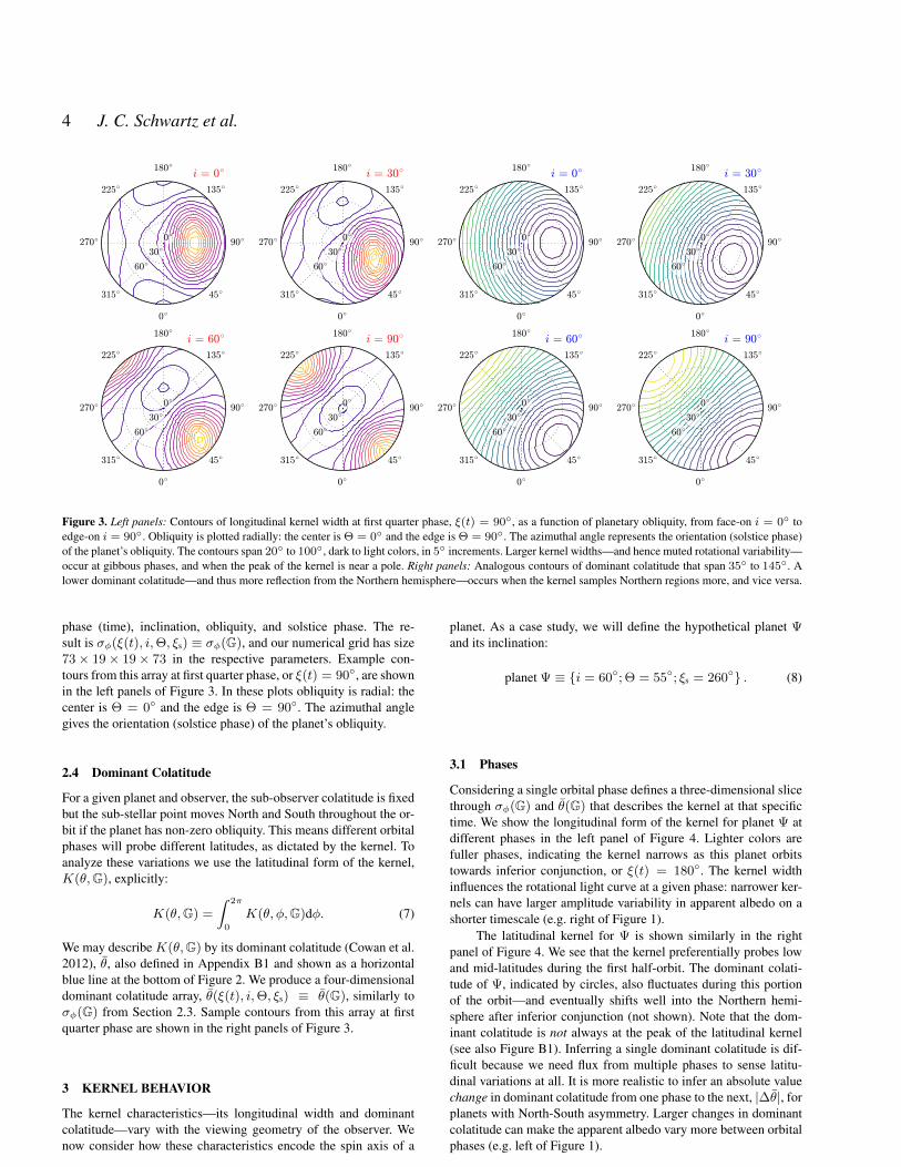
Figure 3. Left panels: Contours of longitudinal kernel width at first quarter phase, ξ(t) = 90, as a function of planetary obliquity, from face-on i = 0 toedge-on i = 90. Obliquity is plotted radially: the center is Θ = 0 and the edge is Θ = 90. The azimuthal angle represents the orientation (solstice phase)of the planet’s obliquity. The contours span 20 to 100, dark to light colors, in 5 increments. Larger kernel widths—and hence muted rotational variability—occur at gibbous phases, and when the peak of the kernel is near a pole. Right panels: Analogous contours of dominant colatitude that span 35 to 145. Alower dominant colatitude—and thus more reflection from the Northern hemisphere—occurs when the kernel samples Northern regions more, and vice versa.

phase (time), inclination, obliquity, and solstice phase. The re-sult is σφ(ξ(t), i,Θ, ξs) ≡ σφ(G), and our numerical grid has size73× 19× 19× 73 in the respective parameters. Example con-tours from this array at first quarter phase, or ξ(t) = 90, are shownin the left panels of Figure 3. In these plots obliquity is radial: thecenter is Θ = 0 and the edge is Θ = 90. The azimuthal anglegives the orientation (solstice phase) of the planet’s obliquity.

2.4 Dominant Colatitude

For a given planet and observer, the sub-observer colatitude is fixedbut the sub-stellar point moves North and South throughout the or-bit if the planet has non-zero obliquity. This means different orbitalphases will probe different latitudes, as dictated by the kernel. Toanalyze these variations we use the latitudinal form of the kernel,K(θ,G), explicitly:

K(θ,G) =

∫ 2π

0

K(θ, φ,G)dφ. (7)

We may describe K(θ,G) by its dominant colatitude (Cowan et al.2012), θ, also defined in Appendix B1 and shown as a horizontalblue line at the bottom of Figure 2. We produce a four-dimensionaldominant colatitude array, θ(ξ(t), i,Θ, ξs) ≡ θ(G), similarly toσφ(G) from Section 2.3. Sample contours from this array at firstquarter phase are shown in the right panels of Figure 3.

3 KERNEL BEHAVIOR

The kernel characteristics—its longitudinal width and dominantcolatitude—vary with the viewing geometry of the observer. Wenow consider how these characteristics encode the spin axis of a

planet. As a case study, we will define the hypothetical planet Ψand its inclination:

planet Ψ ≡ i = 60; Θ = 55; ξs = 260 . (8)

3.1 Phases

Considering a single orbital phase defines a three-dimensional slicethrough σφ(G) and θ(G) that describes the kernel at that specifictime. We show the longitudinal form of the kernel for planet Ψ atdifferent phases in the left panel of Figure 4. Lighter colors arefuller phases, indicating the kernel narrows as this planet orbitstowards inferior conjunction, or ξ(t) = 180. The kernel widthinfluences the rotational light curve at a given phase: narrower ker-nels can have larger amplitude variability in apparent albedo on ashorter timescale (e.g. right of Figure 1).

The latitudinal kernel for Ψ is shown similarly in the rightpanel of Figure 4. We see that the kernel preferentially probes lowand mid-latitudes during the first half-orbit. The dominant colati-tude of Ψ, indicated by circles, also fluctuates during this portionof the orbit—and eventually shifts well into the Northern hemi-sphere after inferior conjunction (not shown). Note that the dom-inant colatitude is not always at the peak of the latitudinal kernel(see also Figure B1). Inferring a single dominant colatitude is dif-ficult because we need flux from multiple phases to sense latitu-dinal variations at all. It is more realistic to infer an absolute valuechange in dominant colatitude from one phase to the next, |∆θ|, forplanets with North-South asymmetry. Larger changes in dominantcolatitude can make the apparent albedo vary more between orbitalphases (e.g. left of Figure 1).

c© 2015 RAS, MNRAS 000, 1–12


−180 −90 0 90 180

Longitude

0.25

0.50

0.75

1.00

Sca

led K

ern

el

0.25 0.50 0.75 1.00Scaled Kernel

0

45

90

135

180

Cola

titu

de

Figure 4. Left: Longitudinal kernel for planet Ψ, defined in Equation 8, at orbital phases from 30 to 150, light to dark shades, in 30 increments. Valuesare scaled to the maximum of the lightest curve. Longitude is measured from each kernel mean. The kernel width decreases as this planet approaches inferiorconjunction, or as color darkens. Right: Analogous latitudinal kernel for Ψ, where the dominant colatitude, indicated by a circle, increases then returns towardsthe equator.

3.2 Time Evolution

Kernel width and dominant colatitude both vary throughout aplanet’s orbit. We investigate this by slicing σφ(G) and θ(G) alonginclination, obliquity, and/or solstice phase. To start, we vary planetΨ’s obliquity and track kernel width as shown in the left panel ofFigure 5. The actual Ψ is denoted by a dashed green line: this planethas a narrow kernel width during the first half-orbit that widenssharply after inferior conjunction. The overlapping traces of differ-ent obliquities make it hard to infer Ψ’s tilt from observations atonly one phase.

We also show tracks of dominant colatitude in the right panelof Figure 5. None overlap until inferior conjunction, when the vari-ation between all obliquities decreases. Planet Ψ is again the dashedgreen line, and near the middle of all the tracks more often than forkernel width. If one already has some knowledge of the viewinggeometry, then Figure 5 indicates at which phases the kernel bestseparates obliquities for Ψ (ξ(t) ≈ 120, in this case).

We can instead vary the solstice phase of Ψ while keeping itsobliquity fixed (not shown). In most cases, solstice phase impactsthe kernel width and dominant colatitude as much as the axial tilt.This is expected, since obliquity is a vector quantity with both mag-nitude and orientation.

4 DISCUSSION

4.1 Measurements

Before continuing in more detail, we must address our assumptionsabout determining the kernel. As noted in Section 2.1, one will notmeasure the kernel directly, but rather infer it by fitting a rotationallight curve (following Cowan et al. 2009; Kawahara & Fujii 2010,2011; Fujii & Kawahara 2012). The planetary inclination and or-bital phase of observation must therefore be known to model thelight curve accurately. Both angles might be obtained with a mix-ture of astrometry on the host star (e.g. SIM PlanetQuest, Unwinet al. 2008), direct-imaging astrometry (Bryden 2015), and/or ra-dial velocity. We will demonstrate constraints on obliquity using

the kernel by assuming inclination and orbital phase have each beenmeasured with 10 uncertainty.

Moreover, extracting the longitudinal width and dominant co-latitude could be difficult in practice. Planets with completely uni-form albedo are obviously not amenable to these methods. Changesin dominant colatitude can only be detected for planets with North-South albedo inhomogeneities. Conversely, one cannot extract thelongitudinal width for planets lacking East-West albedo markings.Even if a planet has suitable albedo asymmetries, photometric un-certainty adds noise to the reflected light measured. Contrast ra-tios 6 10−11 are needed to resolve rotational light curves of anEarth-like exoplanet (Palle et al. 2008), which should be achiev-able by a TPF-type mission with high-contrast coronagraph or star-shade (Ford et al. 2001; Trauger & Traub 2007; Turnbull et al.2012; Cheng-Chao et al. 2015). We will assume kernel widths andchanges in dominant colatitude have been measured with 10 and20 uncertainties apiece, as explained in Appendix B2.

Planetary radii are likewise important, since without them onecannot convert fluxes into apparent albedos (Qui et al. 2003; Cowanet al. 2009). Radii will likely be unknown, but could be approx-imated using mass-radius relations and mass estimates from as-trometry or radial velocity, or inferred from bolometric flux usingthermal infrared direct-imaging (e.g. TPF-I, Beichman et al. 1999;Lawson et al. 2008). Real planets may also have variable albedomaps, short-term from changing clouds and less so long-term fromseasonal changes (Robinson et al. 2010), that could influence theapparent albedo on orbital timescales. These are difficulties thatwill be mitigated with each iteration of photometric detectors andtheoretical models.

4.2 Longitudinal Constraints

For planets with East-West contrast in albedo, one can infer thekernel width at a given phase by fitting a rotational light curve.We can estimate the uncertainty on this width—from rotationalvariations in apparent albedo—by using Monte Carlo simulation(Appendix B2). The upper row of Figure 6 shows confidence re-gions for the obliquity and solstice phase of planet Ψ, usingtwo example kernel widths: 25.2 ± 10.0 at ξ(t) = 120, and

c© 2015 RAS, MNRAS 000, 1–12


0 90 180 270 3600

25

50

75

100

Kern

el W

idth

0 90 180 270 360

0

45

90

135

180

Dom

inant

Cola

titu

de

Orbital Phase

Figure 5. Left: Kernel width for planet Ψ as a function of orbital phase, with obliquity varied in 5 increments. The defined Ψ obliquity, Θ = 55, is thedashed green line; darker and lighter shades of red denote obliquities closer to 0 and 90, respectively. Inferior conjunction occurs at ξ(t) = 180. Thelargest variations are after first quarter phase and inferior conjunction. Right: Analogous dominant colatitude for Ψ, where the largest variation occurs betweenfirst quarter phase and inferior conjunction.

32.8± 10.0 at ξ(t) = 300. We use a normalized Gaussian prob-ability density for each width, and include Gaussian weights dueto uncertainties on inclination and orbital phase, described inSection 4.1.

The true Ψ spin axis is shown in green, and is consistentwith both isolated observations. Kernel width estimates at two or-bital phases still allow all obliquities at 1σ, but exclude nearly19 per cent of spin axes at 3σ. We obtain similar results for otherorbital phases and planet parameters. These examples suggest thatobliquity can be constrained for planets with variable albedo mapsby extracting the kernel width, provided the variations are ontimescales longer than the rotational period.

4.3 Latitudinal & Joint Constraints

With North-South contrast in albedo, one can fit two or morerotational light curves at different phases to infer the kernel’schange in dominant colatitude. We can estimate the uncertaintyon this change—from orbital variations in apparent albedo—withfurther Monte Carlo simulation (Appendix B2). We reapply theprobability density from Section 4.2 to the example absolutevalue change in dominant colatitude, 48.7 ± 20.0, for planet Ψbetween ξ(t) = 120, 300. This constraint is shown as blue re-gions at the lower left of Figure 6. The true Ψ spin axis is againinside the 1σ interval. The distribution is bimodal because we donot know the sign of the variation, meaning whether we are probingmore Northern or Southern latitudes at the later phase.

We infer more with the product distribution of longitudinaland latitudinal constraints, shown as purple regions at the lowerright of Figure 6. This is still bimodal, but the true spin axis isin a high-probability region and obliquities at either extreme canbe excluded at 1σ. A distant observer will know that this planet’sobliquity has probably not been eroded by tides (Heller et al. 2011),and that the planet likely experiences obliquity seasons.

4.4 Pro/Retrograde Rotation

The sign of rotational angular frequency (positive = prograde)does not influence the kernel width or dominant colatitude at agiven phase. Since σφ(G) and θ(G) are identical for retrograderotation, the kernel characteristics will not distinguish progradeand retrograde planets. There is a formal degeneracy for edge-on, zero-obliquity cases: prograde planets with East-oriented mapshave identical light curves to retrograde planets with West-orientedmaps. The path of the kernel peak over either planet is the same,implying the retrograde rotation in an inertial frame is slower(Appendix B3). We show this scenario in the left panel of Figure 7,where the dashed brown line is the difference in prograde and ret-rograde apparent albedo. The orange and black planets are alwaysequally bright because the same map features, in the upper panels,are seen at the same times.

However, the spin direction of oblique planets and/or thoseon inclined orbits may be deduced. Inclinations that are not edge-on most strongly alter a planet’s light curve near inferior conjunc-tion, seen in the center panel of Figure 7: this planet’s propertiesare intermediate between the edge-on, zero obliquity planet andplanet Ψ. While a typical observatory’s inner working angle wouldhide some of the signal, differences of order 0.1 in the apparentalbedo would be detectable at extreme crescent phases. Alterna-tively, higher obliquity causes deviations that—depending on sol-stice phase—can arise around one or both quarter phases. This hap-pens for Ψ in the right panel of Figure 7, where both effects com-bine to distinguish the spin direction at most phases.

Inclination and obliquity influence apparent albedo becausethe longitudinal motion of the kernel peak is not the same at alllatitudes. One can break this spin degeneracy in principle, but wehave not fully explored the pro/retrograde parameter space. In gen-eral, the less inclined and/or oblique a planet is, the more favorablecrescent phases are for determining its spin direction.

c© 2015 RAS, MNRAS 000, 1–12


0

45

90

135

180

225

270

315

0

30

60

0

45

90

135

180

225

270

315

0

30

60

0

45

90

135

180

225

270

315

0

30

60

0

45

90

135

180

225

270

315

0

30

60

0

45

90

135

180

225

270

315

0

30

60

× =

→

Figure 6. Confidence regions for planet Ψ’s spin axis using example data described in Sections 4.2 and 4.3: longitudinal widths of the kernel in red, theabsolute value change in dominant colatitude in blue, and the joint constraints in purple. Obliquity is plotted radially: the center is Θ = 0 and the edge isΘ = 90. The azimuthal angle represents the planet’s solstice phase. Regions up to 3σ are shown, where darker bands are more likely. Kernel widths haveassumed 10 uncertainty, and match Ψ at ξ(t) = 120, 300 in the upper left and center, respectively. These individual red constraints are combined at theupper right. The change in dominant colatitude has an assumed 20 uncertainty, while inclination and orbital phases each have assumed 10 uncertainty. Thegreen circles are the true Ψ spin axis. Obtaining just a few single-epoch observations of a planet can significantly constrain both the magnitude and orientationof its spin axis.

5 CONCLUSIONS

We have performed numerical experiments to study the problemof inferring a planet’s obliquity based solely on time-resolved pho-tometry. We have demonstrated that a planet’s obliquity will in-fluence its light curve in two distinct ways, and that we can an-alyze the kernel of reflection independent of the planet’s albedomap. This kernel—the combination of stellar illumination and ob-server visibility—has a peak, a longitudinal width, and a dominantcolatitude that vary in time, are functions of viewing geometry, andencode the planet’s obliquity. As long as a planet is not completelyuniform, one can infer properties of both the kernel and albedomap. These characteristics help one determine the planet’s spin di-rection and constrain both components of its spin axis, including formaps that are East-West uniform (e.g. Jupiter-like) or North-Southuniform (e.g. beach ball-like). Curiously, we find that kernel widthis more useful in general, meaning obliquity is typically easier toinfer from rotational rather than orbital information.

Moreover, one only needs to monitor a planet at a limited num-ber of epochs to determine its obliquity. In our case study, we usedobservations at just two distinct phases to reduce the possible spinaxes of planet Ψ by about 75 per cent at 1σ. Additional observa-tions of order a week—rather than many months—could well con-strain the true components, good news for inferring the obliquity ofterrestrial exoplanets during direct-imaging surveys. We envision atriage approach for such missions: planets that vary in brightnessthe most, and thus have the easiest kernels to extract, will be thefirst for follow-up observations.

ACKNOWLEDGMENTS

The authors thank the anonymous referee for important sugges-tions that improved the paper, and the International Space Sci-ence Institute (Bern, CH) for hosting their research workshop, “TheExo-Cartography Inverse Problem.” Participants included Ian M.Dobbs-Dixon (NYUAD), Ben Farr (U. Chicago), Will M. Farr (U.Birmingham), Yuka Fujii (TIT), Victoria Meadows (U. Washing-ton), and Tyler D. Robinson (UC Santa Cruz). JCS was funded byan NSF GK-12 fellowship, and as a Graduate Research Trainee atMcGill University.

REFERENCES

Barnes J. W., Fortney J. J., 2003, The Astrophysical Journal, 588, 545Beichman C. A., Woolf N., Lindensmith C., 1999, The Terrestrial Planet

Finder (TPF): a NASA Origins Program to search for habitable plan-ets/the TPF Science Working Group; edited by CA Beichman, NJWoolf, and CA Lindensmith.[Washington, DC]: National Aeronauticsand Space Administration; Pasadena, Calif.: Jet Propulsion Laboratory,California Institute of Technology,[1999](JPL publication; 99-3), 1

Bryden G., 2015, IAU General Assembly, 22, 58195Carter J. A., Winn J. N., 2010, The Astrophysical Journal, 709, 1219Cheng-Chao L., De-Qing R., Jian-Pei D., Yong-Tian Z., Xi Z., Gang Z.,

Zhen W., Rui C., 2015, Research in Astronomy and Astrophysics, 15,453

Cowan N. B., Abbot D. S., Voigt A., 2012, The Astrophysical JournalLetters, 752, L3

Cowan N. B., Agol E., Meadows V. S., Robinson T., Livengood T. A.,

c© 2015 RAS, MNRAS 000, 1–12


0 90 180 270 360

0.25

0.00

0.25

0.50

0.75

Appare

nt

Alb

edo

0 90 180 270 360

Orbital Phase

0.25

0.00

0.25

0.50

0.75

0 90 180 270 360

0.25

0.00

0.25

0.50

0.75

Figure 7. Apparent albedo as a function of orbital phase, shown for an edge-on, zero obliquity planet at left, planet Ψ at right, and an intermediate planetin the center. The black and orange curves correspond to prograde and retrograde rotation, respectively. The differences in apparent albedo are the dashedbrown lines. A low rotational frequency is used for clarity; inferior conjunction occurs at ξ(t) = 180. The albedo maps are color-coded at top, where arrowsindicate spin direction and the prime meridians are centered. Note that these maps are East-West reflections of each other. The edge-on, zero-obliquity curvesare identical, while the curves for the intermediate planet and Ψ grow more distinct. Edge-on, zero-obliquity planets are hopeless, but one can distinguishpro/retrograde rotation for inclined, oblique planets by monitoring their brightness, particularly near crescent phases.

Deming D., Lisse C. M., A’Hearn M. F., Wellnitz D. D., Seager S., et al.,2009, The Astrophysical Journal, 700, 915

Cowan N. B., Fuentes P. A., Haggard H. M., 2013, Monthly Notices of theRoyal Astronomical Society, 434, 2465

Cowan N. B., Strait T. E., 2013, The Astrophysical Journal Letters, 765,L17

De Kok R., Stam D., Karalidi T., 2011, The Astrophysical Journal, 741,59

Dones L., Tremaine S., 1993, Icarus, 103, 67Ford E., Seager S., Turner E., 2001, Nature, 412, 885Fujii Y., Kawahara H., 2012, The Astrophysical Journal, 755, 101Fujii Y., Kawahara H., Suto Y., Fukuda S., Nakajima T., Livengood T. A.,

Turner E. L., 2011, The Astrophysical Journal, 738, 184Fujii Y., Kawahara H., Suto Y., Taruya A., Fukuda S., Nakajima T., Turner

E. L., 2010, The Astrophysical Journal, 715, 866Gaidos E., Williams D., 2004, New Astronomy, 10, 67Heller R., Leconte J., Barnes R., 2011, Astronomy & Astrophysics, 528,

A27Kawahara H., 2012, The Astrophysical Journal Letters, 760, L13Kawahara H., Fujii Y., 2010, The Astrophysical Journal, 720, 1333Kawahara H., Fujii Y., 2011, The Astrophysical Journal Letters, 739, L62Kokubo E., Ida S., 2007, The Astrophysical Journal, 671, 2082Kouveliotou C., Agol E., Batalha N., Bean J., Bentz M., Cornish N.,

Dressler A., Figueroa-Feliciano E., Gaudi S., Guyon O., et al., 2014,arXiv preprint arXiv:1401.3741

Laskar J., 1994, Astronomy and Astrophysics, 287, L9Laskar J., Joutel F., Robutel P., 1993, Nature, 361, 615Laskar J., Robutel P., Joutel F., Gastineau M., Correia A., Levrard B.,

2004, Astronomy & Astrophysics, 428, 261Lawson P., Lay O., Martin S., Peters R., Gappinger R., Ksendzov A.,

Scharf D., Booth A., Beichman C., Serabyn E., et al., 2008, in SPIEAstronomical Telescopes+ Instrumentation Terrestrial planet finder in-terferometer: 2007-2008 progress and plans. pp 70132N–70132N

Miguel Y., Brunini A., 2010, Monthly Notices of the Royal AstronomicalSociety, 406, 1935

Nikolov N., Sainsbury-Martinez F., 2015, The Astrophysical Journal, 808,57

Oakley P., Cash W., 2009, The Astrophysical Journal, 700, 1428Palle E., Ford E. B., Seager S., Montanes-Rodrıguez P., Vazquez M., 2008,

The Astrophysical Journal, 676, 1319Pierrehumbert R. T., 2010, Principles of planetary climate. Cambridge

University PressPostman M., Traub W., Krist J., Stapelfeldt K., Brown R., Oegerle W., Lo

A., Clampin M., Soummer R., Wiseman J., et al., 2009, arXiv preprintarXiv:0911.3841

Qui J., Goode P., Palle E., Yurchyshyn V., Hickey J., Montanes-RodrıguezP., Chu M., Kolbe E., Brown C., Koonin S., 2003, Journal of GeophysicalResearch, pp 12–1

Robinson T. D., Ennico K., Meadows V. S., Sparks W., Bussey D. B. J.,Schwieterman E. W., Breiner J., 2014, The Astrophysical Journal, 787,

c© 2015 RAS, MNRAS 000, 1–12


171Robinson T. D., Meadows V. S., Crisp D., 2010, The Astrophysical Journal

Letters, 721, L67Schlichting H. E., Sari R., 2007, The Astrophysical Journal, 658, 593Seager S., Hui L., 2002, The Astrophysical Journal, 574, 1004Spiegel D. S., Menou K., Scharf C. A., 2009, The Astrophysical Journal,

691, 596Trauger J. T., Traub W. A., 2007, Nature, 446, 771Turnbull M. C., Glassman T., Roberge A., Cash W., Noecker C., Lo A.,

Mason B., Oakley P., Bally J., 2012, Publications of the AstronomicalSociety of the Pacific, 124, 418

Unwin S. C., Shao M., Tanner A. M., Allen R. J., Beichman C. A., BoboltzD., Catanzarite J. H., Chaboyer B. C., Ciardi D. R., Edberg S. J., et al.,2008, Publications of the Astronomical Society of the Pacific, 120, 38

Williams D. M., Gaidos E., 2008, Icarus, 195, 927Williams D. M., Kasting J. F., 1997, Icarus, 129, 254Williams D. M., Pollard D., 2003, International Journal of Astrobiology,

2, 1

APPENDIX A: VIEWING GEOMETRY

A1 General Observer

The time-dependence of the kernel is contained in the sub-observer andsub-stellar angles: θo, φo θs, φs. Since they do not depend on planetarylatitude or longitude, these four angles may be factored out of the kernelintegrals. However, the light curves are still functions of time, so we derivethe relevant dependencies here.

In particular, we compute the sub-stellar and sub-observer locationsfor planets on circular orbits using seven parameters. Three are intrinsic tothe system: rotational angular frequency, ωrot ∈ (−∞,∞), orbital angularfrequency, ωorb ∈ (0,∞), and obliquity, Θ ∈ [0, π/2]. Rotational fre-quency is measured in an inertial frame, where positive values are progradeand negative denotes retrograde rotation (for comparison, the rotational fre-quency of Earth is ω⊕

rot ≈ 2π/23.93 hr−1). Two more parameters are ex-trinsic and differ for each observer: orbital inclination, i ∈ [0, π/2] wherei = 90 is edge-on, and solstice phase, ξs ∈ [0, 2π), which is the orbitalangle between superior conjunction and the maximum Northern excursionof the sub-stellar point. The remaining parameters are extrinsic initial condi-tions: the starting orbital position, ξ0 ∈ [0, 2π), and the initial sub-observerlongitude, φo(0) ∈ [0, 2π). These parameters are illustrated in Figure A1;other combinations are possible.

We define the orbital phase of the planet as ξ(t) = ωorbt+ξ0. Withoutloss of generality we may set the first initial condition as ξ0 = 0, whichputs the planet at superior conjunction when t = 0. With no precession thesub-observer colatitude is constant,

θo(t) = θo. (A1)

This angle can be expressed in terms of the inclination, obliquity, and sol-stice phase using the spherical law of cosines (bottom of Figure A1):

cos θo = cos i cos Θ + sin i sin Θ cos ξs, (A2)

sin θo =√

1− cos2 θo. (A3)

The sub-observer longitude decreases linearly with time for prograde rota-tion, as we define longitude increasing to the East:

φo(t) = −ωrott+ φo(0). (A4)

The prime meridian (φp ⇒ φ = 0) is a free parameter, which we defineto run from the planet’s North pole to the sub-observer point at t = 0. Thissets the second initial condition, namely φo(0) = 0, and means

cosφo = −ωrott, (A5)

sinφo =√

1− cos2 φo. (A6)

Hence, the time evolution of the sub-observer point is specified by its colat-itude and the rotational angular frequency.

The sub-stellar position is more complex for planets with non-zero

Figure A1. The upper panel shows a side view of the gen-eral planetary system. The rotational and orbital angular frequenciesωrot, ωorb, inclination i, obliquity Θ, sub-observer colatitude θo, andobserver viewing direction ˆ are indicated. The lower panel is an isomet-ric view, showing the solstice phase ξs. Superior conjunction occurs alongthe positive x-axis. Note the inertial coordinates, how they relate to theobserver’s viewpoint and planet’s spin axis, and the angles between thesevectors.

obliquity. Consider an inertial Cartesian frame centered on the host starwith fixed axes as follows: the z-axis is along the orbital angular frequency,z = ωorb, while the x-axis points towards superior conjunction. The y-axisis then orthogonal to this plane using y = z × x (bottom of Figure A1). Inthese inertial coordinates, the unit vector from the planet center towards thehost star is rps = − cos ξx − sin ξy. The corresponding unit vector fromthe star towards the observer is ˆ = − sin ix + cos iz. Our approach is toexpress everything in the inertial coordinate system, then find the sub-stellarpoint with appropriate dot products.

For the planetary surface, we use a second coordinate system fixedto the planet. We align the zp-axis with the rotational angular frequency,zp = ωrot, while the xp-axis is set by our choice for the prime meridian(and initial sub-observer longitude.) The final axis, yp, is again determinedby taking yp = zp × xp. We proceed in two steps, first finding the plan-etary axes when t = 0, then using the planet’s rotation to describe theseaxes at any time.

Since we disregard precession, the planet’s rotation axis is time-independent:

zp = ωrot = − cos ξs sin Θx− sin ξs sin Θy + cos Θz. (A7)

The sub-observer point is on the prime meridian when t = 0, so that

yp(0) =zp × ˆ

sin θo. (A8)

Computing this we find

yp(0) =1

sin θo

[− cos i sin ξs sin Θx

+ (cos i cos ξs sin Θ− sin i cos Θ)y

− sin i sin ξs sin Θz].

(A9)

The starting xp-axis is then found by taking yp(0)× zp. The result is sim-

c© 2015 RAS, MNRAS 000, 1–12


plified by using Equation A2:

xp(0) =1

sin θo

[(cos ξs sin Θ cos θo − sin i)x

+ sin ξs sin Θ cos θoy

+ sin Θ(cos i sin Θ− sin i cos ξs cos Θ)z].

(A10)

We can now find the planetary axes, in terms of the inertial axes, atany time by rotating Equations A9 and A10 about the zp-axis:

xp = cos(ωrott)xp(0) + sin(ωrott)yp(0), (A11)

yp = − sin(ωrott)xp(0) + cos(ωrott)yp(0). (A12)

The sub-stellar angles in the planetary coordinates may then be extractedfrom the relations

sin θs cosφs = rps · xp, (A13)

sin θs sinφs = rps · yp, (A14)

cos θs = rps · zp, (A15)

resulting in:

cos θs = sin Θ cos [ξ − ξs] , (A16)

sin θs =

√1− sin2 Θ cos2 [ξ − ξs], (A17)

cosφs =cos(ωrott)a(t) + sin(ωrott)b(t)√

1− cos2 θo√

1− sin2 Θ cos2 [ξ − ξs], (A18)

sinφs =− sin(ωrott)a(t) + cos(ωrott)b(t)√

1− cos2 θo√

1− sin2 Θ cos2 [ξ − ξs], (A19)

where the factors a(t) and b(t) are given by

a(t) =

sin i cos ξ − cos θo sin Θ cos [ξ − ξs], (A20)

b(t) =

sin i sin ξ cos Θ− cos i sin Θ sin [ξ − ξs]. (A21)

Note that when θs = 0, π, the sub-stellar longitude can be set arbitrarilyto avoid dividing by zero in Equations A18 and A19.

A2 Polar Observer

Equations A18 and A19 for the sub-stellar longitude apply to most ob-servers. However, the definition of yp(0) in Equation A8 fails when thesub-observer point coincides with one of the planet’s poles. Two alternatedefinitions can be used in these situations.

Case 1: If the sub-stellar point will not pass over the poles duringorbit, we may define

yp(0) = −y, (A22)

so that

xp(0) = yp(0)× zp = − cos Θx− cos ξs sin Θz. (A23)

This results in

cosφs =cosωrot cos ξ cos Θ + sinωrot sin ξ√

1− sin2 Θ cos2 [ξ − ξs], (A24)

sinφs =− sinωrot cos ξ cos Θ + cosωrot sin ξ√

1− sin2 Θ cos2 [ξ − ξs]. (A25)

Case 2: However, if the sub-stellar point will pass over the poles dur-ing orbit, we define instead

xp(0) = z, (A26)

such that

yp(0) = zp × xp(0) = cos ξsy. (A27)

This produces

cosφs =− sinωrot sin ξ cos ξs√1− sin2 Θ cos2 [ξ − ξs]

, (A28)

sinφs =− cosωrot sin ξ cos ξs√1− sin2 Θ cos2 [ξ − ξs]

. (A29)

These special cases only impact the sub-stellar longitude: expressionsfor the other angles are unchanged. As with a general observer, the Case 2sub-stellar longitude may be set arbitrarily whenever θs = 0, π.

A3 Zero Obliquity

For non-oblique planets, Θ = 0, the sub-observer colatitude satisfies

cos θo = cos i, (A30)

sin θo = sin i, (A31)

while the sub-stellar angles become

cos θs = 0, (A32)

sin θs = 1, (A33)

cosφs =cos(ωrott)c(t) + sin(ωrott)d(t)

√1− cos2 i

, (A34)

sinφs =− sin(ωrott)c(t) + cos(ωrott)d(t)

√1− cos2 i

, (A35)

where c(t) and d(t) are given by

c(t) = sin i cos ξ, (A36)

d(t) = sin i sin ξ. (A37)

The sub-stellar longitude is therefore

cosφs =cos(ωrott) sin i cos ξ + sin(ωrott) sin i sin ξ

√1− cos2 i

= cos(ωrott) cos ξ + sin(ωrott) sin ξ

= cos(ξ − ωrott),

(A38)

sinφs =− sin(ωrott) sin i cos ξ + cos(ωrott) sin i sin ξ

√1− cos2 i

= − sin(ωrott) cos ξ + cos(ωrott) sin ξ

= sin(ξ − ωrott).

(A39)

In other words, θo = i, φo = φo(0)− ωrott, θs = 0, and φs = ξ − ωrott.

APPENDIX B: KERNEL DETAILS

B1 Characteristics

An important measure of the longitudinal kernel is its width, σφ, as shownin the left panel of Figure B1. We treat this width mathematically as a stan-dard deviation. Since K(φ,G) is on a periodic domain, we minimize thevariance for each geometry with respect to the grid location of the primemeridian, φp:

σ2φ = min

[∫ 2π

0

(φ

′− φ

)2K(φ)dφ

]φp

, (B1)

where K(φ) = K(φ)/∫K(φ)dφ is the spherically normalized longitudi-

nal kernel, φ′ ≡ φ+ φp, and φ is the mean longitude:

φ =

∫ 2π

0φ

′K(φ)dφ. (B2)

All longitude arguments and separations in Equations B1 and B2 wraparound the standard domain [0, 2π). Also note the unprimed arguments in-side the kernel: these make computing the variance simpler. The minimumvariance determines the standard deviation of the kernel, and thus width, fora given geometry.

c© 2015 RAS, MNRAS 000, 1–12


0 90 180 270 360

Longitude

0.05

0.10

0.15

0.20

Kern

el

0.3 0.6 0.9Kernel

0

45

90

135

180

Cola

titu

de

Figure B1. Left: Longitudinal kernels of a planet with different obliquities at first quarter phase, ξ(t) = 90, where ξs = 225 and i = 60. The curvesshow 0 to 90 obliquity in 15 increments, where lighter shades of red indicate higher tilts. The kernel width of this planet changes as obliquity increases.Right: Analogous latitudinal kernels that indicate dominant colatitude, shown as a circle, also changes as obliquity increases.

The dominant colatitude is similarly important for the latitudinal ker-nel, as shown in the right panel of Figure B1. Cowan et al. (2012) definedthe dominant colatitude, θ, for a given geometry:

θ =

∮θK(θ, φ)dΩ, (B3)

where K(θ, φ) = K(θ, φ)/∮K(θ, φ)dΩ is the normalized kernel.

Equation B3 is equivalent to

θ =

∫ π

0θK(θ) sin θdθ, (B4)

where K(θ) = K(θ)/∫K(θ) sin θdθ is the spherically normalized lati-

tudinal kernel. The dominant colatitude is the North-South region that getssampled most by the kernel (e.g. the circles in Figure B1.)

B2 Albedo Variations

Figure 1 demonstrates that obliquity is related to—though not explicitlygiven by—both rotational and orbital variations of a planet’s apparentalbedo. We use a Monte Carlo approach to quantify these relations, sim-ulating planets with different maps and viewing geometries. We generatealbedo maps from spherical harmonics, Ym` (θ, φ), on the same 101× 201grid in colatitude and longitude from Section 2.2:

A(θ, φ) =

`max∑`=0

∑m=−`

Cm` Ym` (θ, φ), (B5)

where `max is chosen to be 3, each coefficient Cm` is randomly drawnfrom the standard normal distribution, and the composite map is scaled tothe Earth-like range [0.1, 0.8]. Rotational and orbital changes in brightnessare caused by East-West and North-South albedo markings, respectively, sowe make three types of maps: East-West featured with Cm` (m 6= `) = 0,North-South featured with Cm` (m 6= 0) = 0, or no Cm` restrictions. Forall maps with East-West features, we randomly offset the prime meridian.We generate 5,000 maps of each type.

For each map we randomly select an obliquity, solstice phase, inclina-tion, and two orbital phases. Since inclination and orbital phase can be mea-sured independent of photometry, we choose inclinations similar to planetΨ, i ∈ [50,70], and orbital phases ξ1, ξ2 with ∆ξ ∈ [110, 130].Both phases are also at least 30 from superior and inferior conjunction,which conservatively mimics an inner working angle at the selected in-clinations. We assume the planet’s rotational and orbital frequencies areknown (Palle et al. 2008; Oakley & Cash 2009), and use the Earth-like

ratio ωrot/ωorb = 360. We divide roughly one planet rotation centered oneach orbital phase into 51 time steps, then define the normalized amplitudeof rotational and orbital albedo variations, Λrot and Λorb, as:

Λrot =Ahighξ1−Alow

ξ1

Aξ1, (B6)

Λorb = |Aξ1 − Aξ2 |(Aξ1 + Aξ2

2

)−1

, (B7)

where Ahighξ1

and Alowξ1

are the extreme apparent albedos around the firstphase, and A is the mean apparent albedo of all time steps around a givenphase. For each computed Λrot and Λorb, we calculate the correspond-ing kernel width and absolute value change in dominant colatitude, fromAppendix B1. Figure B2 shows the resulting distributions, where rotationaland orbital information is colored red and blue, respectively. We find similarresults when relaxing constraints on the inclination and orbital phases.

We can estimate uncertainties on values of σφ and |∆θ| using thesedistributions. The mean rotational and orbital variations are approximately0.54 and 0.21 each; the average kernel width and change in dominant co-latitude are both roughly 38. For the full distributions we find standarddeviations of about 17 on σφ and 24 on |∆θ|, but roughly 5 and 7

respectively for large variations. To demonstrate constraints on obliquity,we consider a typical scenario and assume we have single-epoch observa-tions, explicitly at ξ(t) = 120, 300, with the mean variations (0.54and 0.21) from our distributions. The sets of samples near these variationsshow about 10 and 20 standard deviations apiece in the kernel width andchange in dominant colatitude, which we use as example uncertainties inFigure 6.

B3 Peak Motion

Equations C1 and C2 from Cowan et al. (2009) describe the motion of thekernel peak, where specular reflection occurs, for any planetary system.These equations can be written for edge-on, zero obliquity planets usingSection A3:

cos θspec =1 + cos i√2(1 + cos i)

, (B8)

c© 2015 RAS, MNRAS 000, 1–12


0.0 0.5 1.0 1.5 2.0Rotational Albedo Variation

0

25

50

75

100

Kern

el W

idth

0.0 0.2 0.4 0.6 0.8 1.0 1.2 1.4Orbital Albedo Variation

0

25

50

75

100

Change in D

om

inant

Cola

titu

de

Figure B2. Kernel-albedo distributions for two sets of 10,000 planets generated via Monte Carlo, comparing rotational properties in red and orbital propertiesin blue. Changes in dominant colatitude are absolute values, and planets are binned in 0.1 × 2 regions in both panels. Each color scale is logarithmic: thedarkest red and blue bins contain 230 and 279 planets, respectively. The scatter in either kernel characteristic decreases as the corresponding albedo variationrises. We can estimate the uncertainty on a kernel width or change in dominant colatitude by analyzing these distributions.

tanφspec =sin(ξ − ωrott) + sin(φo(0)− ωrott)

cos(ξ − ωrott) + cos(φo(0)− ωrott)

=sin(ωorbt− ωrott) + sin(φo(0)− ωrott)

cos(ωorbt− ωrott) + cos(φo(0)− ωrott).

(B9)

When finding φspec from Equation B9, the two-argument arctangent mustbe used to ensure φspec ∈ [−π, π). This also means it is difficult to simplifythe equation with trigonometric identities.

Instead, we can explicitly write the argument of Equation B9 in termsof the first meridian crossing, ξm, the earliest orbital phase after superiorconjunction that the kernel peak recrosses the prime meridian:

φspec(ξ; ξm) = ∓π

2

(4ξ

ξm+

[1− sgn

(cos

ξ

2

)]), (B10)

where the leading upper sign applies to prograde rotation and vice versa.The first meridian crossing is related to the planet’s frequency (or period)ratio by ∣∣∣∣ ωrot

ωorb

∣∣∣∣ =

∣∣∣∣Porb

Prot

∣∣∣∣ =1

2

(4π

ξm± 1

), (B11)

while the number of solar days per orbit is

Nsolar =

∣∣∣∣ ωrot

ωorb

∣∣∣∣∓ 1, (B12)

following the same sign convention. Note that the frequency/period ratiosand the number of solar days do not have to be integers. We reiterate thatEquations B8 through B12 apply to edge-on, zero obliquity planets.

Equation B11 gives two frequency ratios for each first meridian cross-ing, one prograde and another retrograde that is smaller in magnitudeby unity. Equation B12 then says the corresponding difference in solardays is unity but reversed, making the longitudes of both kernel peaks inEquation B10 analogous at each orbital phase. These two versions of theplanet have East-West mirrored albedo maps and identical light curves: theyare formally degenerate. An inclined, oblique planet has pro/retrograde ver-sions that could be distinguished, as discussed in Section 4.4.

This paper has been typeset from a TEX/ LATEX file prepared by theauthor.

c© 2015 RAS, MNRAS 000, 1–12

inferring planetary obliquity using rotational &...

Documents