information-flow and data-flow analysis of...
TRANSCRIPT
Information-Flow and Data-Flow Analysis of while-Programs
JEAN-FRANC06 BERGERETTI and BERNARD A. CARRY
University of Southampton
Until recently, information-flow analysis has been used primarily to verify that information trans- mission between program variables cannot violate security requirements. Here, the notion of infor- mation flow is explored as an aid to program development and validation.
Information-flow relations are presented for while-programs, which identify those program statements whose execution may cause information to be transmitted from or to particular input, internal, or output values. It is shown with examples how these flow relations can be helpful in writing, testing, and updating programs; they also usefully extend the class of errors which can be detected automatically in the “static analysis” of a program.
Categories and Subject Descriptors: D.2.2 [Software Engineering]: Tools and Techniques; D.2.4 [Software Engineering]: Program Verification; D.2.5 [Software Engineering]: Testing and Debugging; D.2.6 [Software Engineering]: Programming Environments
General Terms: Information flow, data flow, analysis of programs, automatic error detection, debug- ging, software maintenance
1. INTRODUCTION
As was noted by the authors of Euclid [ 191, “. . . most programs presented to verifiers are actually wrong; considerable time can be wasted looking for proofs of incorrect programs before discovering that debugging is still needed. This problem can be reduced (although not eliminated) by judicious testing, which is generally the most efficient way to demonstrate the presence of bugs. . . .”
The testing process can be assisted, for instance, by run-time checks of assertions [ 191, but in general it remains a rather haphazard way of revealing the errors in a program. For this reason, there is currently much interest in extending program flow analysis methods, such as data-flow analysis, to enable these methods to detect a larger class of errors than they can uncover at the present time [18].
This paper describes some information-flow relations that are easily con- structed for a while-program and that are helpful both in program testing and in checking the consistency of assertions with a program text. They also usefully
Authors’ address: Department of Electronics and Information Engineering, University of Southamp- tom, Southampton SO9 5NH, England. Permission to copy without fee all or part of this material is granted provided that the copies are not made or distributed for direct commercial advantage, the ACM copyright notice and the title of the publication and its date appear, and notice is given that copying is by permission of the Association for Computing Machinery. To copy otherwise, or to republish, requires a fee and/or specific permission. 0 1985 ACM 0164-0925/85/0100-0037 $00.75
ACM Transactions on Programming Languages and Systems, Vol. 7, No. 1, January 1985, Pages 37-61.
38 l J.-F. Bergeretti and B. A. Car&
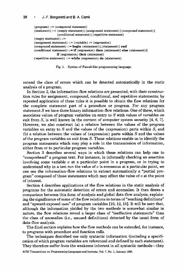
(program) ::= (compound statement) (statement) : : = (empty statement) 1 (assignment statement) 1 (compound statement) 1
(conditional statement) 1 (repetitive statement) (empty statement) ::= (assignment statement) ::= (variable) := (expression) (compound statement) : : = begin (statement) (; (statement) ) end (conditional statement) : := if (expression) then (statement) else (statement) 1
if (expression) then (statement) (repetitive statement) : : = while (expression) do (statement)
Fig. 1. Syntax of Pascal-like programming language.
extend the class of errors which can be detected automatically in the static analysis of a program.
In Section 2, the information-flow relations are presented, with their construc- tion rules for assignment, compound, conditional, and repetitive statements; by repeated application of these rules it is possible to obtain the flow relations for the complete statement part of a procedure or program. For any program statement S we have three binary information-flow relations. One of these, which associates values of program variables on entry to S with values of variables on exit from S, is well known in the context of computer system security [4, 6, 71. However, we also construct (a) a relation between the values of the program variables on entry to S and the values of the (expression) parts within S, and (b) a relation between the values of (expression) parts within S and the values of the program variables on exit from S. These relations enable us to identify the program statements which may play a role in the transmission of information, either from or to particular program variables.
Section 3 describes several ways in which these relations can help one to “comprehend” a program text. For instance, in informally checking an assertion involving some variable u at a particular point in a program, or in trying to understand why in a test run the value of u is erroneous at a particular point, we can use the information-flow relations to extract automatically a “partial pro- gram” composed of those statements which may affect the value of u at the point of interest.
Section 4 describes applications of the flow relations in the static analysis of programs for the automatic detection of errors and anomalies. It then draws a comparison between this form of analysis and global data-flow analysis, explain- ing the significance of some of the flow relations in terms of “reaching definitions” and “upward-exposed uses” of program variables [ 10,12,15]. It will be seen that, although the information yielded by the two methods is somewhat similar in nature, the flow relations reveal a larger class of “ineffective statements” than the class of anomalies (i.e., unused definitions) detected by the usual form of data-flow analysis.
The final section explains how the flow methods can be extended, for instance, to programs with procedure and function calls.
The techniques described use only syntactic information (including a specifi- cation of which program variables are referenced and defined by each statement). They therefore suffer from the weakness inherent in all syntactic methods-they
ACM Transactions on Programming Languages and Systems, Vol. 7, No. 1, January 1985.

Information-Flow and Data-Flow Analysis of while-Programs 39
T F e
b A
4 (a) b) (4
Fig. 2. Control-flow graphs of program statements. (a) if e then A else B. (b) if e then A. (c) while e do A.
are “conservative,” in that they may indicate possible data dependencies even where the program semantics preclude these. Nevertheless, as the examples demonstrate, the flow relations provide a useful aid to program analysis.
2. INFORMATION-FLOW RELATIONS
For ease of exposition we first present our methods of information- and data- flow analysis with reference to the simple Pascal-like programming language whose syntax is given in Figure 1. We need not specify the grammar or semantics of expressions, but it is assumed that the evaluation of an expression has no side effects.
The control flow in any program statement S in this language can be repre- sented by a control-flow graph G(S), with one node corresponding to each assignment statement in S, one node corresponding to the (expression) part of each conditional and repetitive statement in S, and arcs representing the possible transfers of control (see Figure 2).
We denote by V the set of all variables in a program, and we let E denote the set of all instances of an (expression) in the program. Also, for each expression e E E, we let I(e) stand for the set of all variables which appear in e.
2.1 Defined and Preserved Variables
We say that (the execution of) a statement S may define a variable v if S contains any assignments to v, and we denote the set of variables which S may define by Ds. Also, we say that a statement S may preserve (the value of) a variable v if in G(S) there exists a path from the entry to the exit which is definition-clear for v (i.e., which does not traverse any assignments to v). We denote the set of variables which S may preserve by Ps.
The sets DS and PS can be constructed immediately for an empty statement (these are defined by formulas (Tl) and (T2) of Table I’) and for an assignment statement (see (T6) and (T7)). If S is a sequence of statements (A; B; . . .), then the sets Ds and Ps are easily constructed from the sets DA, DB, . . . and PA, Pe, . . . associated with the constituents of S (see (Tll) and (T12)). The same is true
’ Table I contains formulas (Tl)-(T30).
ACM Transactions on Programming Languages and Systems, Vol. 7, No. 1, January 1985.
40 l J.-F. Bergeretti and B. A. Carr6
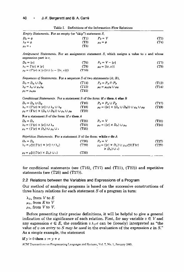
Table I. Definitions of the Information-FIow Relations
Empty Statements. For an empty (or “skip”) statement S,
Ds=@ (Tl) Ps= v (T2) x.9 = 6 (T3) LL9 = dJ (T4) PS = 1 (7’5)
Assignment Statements. For an assignment statement S, which assigns a value to v and whose expression part is e,
Ds = Iv) (T6) Ps= V-Iv) AS = r(e) X (e) (‘I%) PS = I@, u)l PS = (r(e) x lul) U (L- lb, VII) (T10)
Sequences of Statements. For a sequence S of two statements (A; B),
Ds=D*uDs (Tll) Ps = Pa n P.9 b=~AupAxB (773) &9=,&4pBu~B
PS = PAPB (7’15)
Conditional Statements. For a statement S of the form: if e then A else B
Ds=DAuDB V16) Ps = Pn u Ps XS = (r(e) X {e)) U AA U A* (T18) PS = (lel X (DA U DB)) U P.A U PB PS = (r(e) x (DA U Ds)) U PA U PB (7’2’3 For a statement S of the form: if e then A
Ds=D., UW Ps = v X.9 = (r(e) x 14) U X,4 w3) PCS = (14 x DA) U PA ps = (r(e) x DA) U pa U L 0’25)
Repetitive Statements. For a statement S of the form: while e do A
Ds=D, U-3 Ps= v AS= P:((r(e) x iel) u AA) U-3) PS= (14 x DA) U hLApX((r(e)
X DA) U 1) PS = pX((r(e) x DA) U 1) 030)
W7) (T9)
U’12) W4)
V17) UW
U-27) VW
for conditional statements (see (T16), (T17) and (T21), (T22)) and repetitive statements (see (T26) and (T27)).
2.2 Relations between the Variables and Expressions of a Program
Our method of analyzing programs is based on the successive constructions of three binary relations for each statement S of a program in turn:
XL+, from V to E ~3, from E to V ps, from V to V.
Before presenting their precise definitions, it will be helpful to give a general indication of the significance of each relation. First, for any variable u E V and any expression e E E, the condition IJ hse can be (loosely) interpreted as “the value of IJ on entry to S nay be used in the evaluation of the expression e in S.” As a simple example, the statement
ify>Othenx:=y+z
ACM Transactions on Programming Languages and Systems, Vol. 7, No. 1, January 1985.

Information-Flow and Data-Flow Analysis of while-Programs 41
contains two expressions (y > 0 and y + z). The value of y on entry to this statement may be used in evaluating both expressions; the entry value of z may be used in evaluating the second expression only. For the statement S consisting of two assignments
beginx:=y+z;w:=2:xend
the values of y and z on entry to S may be used in evaluating the expression y + z; we also say that these values may be used in evaluating the second expression 2 * X, since the value of the first expression determines the value of the variable x in the second. We do not say that the value of x on entry to S may be used in the evaluation of the second expression, since this entry value is “killed” by the first assignment statement.
As a final example, let us consider the compound statement
beginifx>Otheny:=l;z:=2*yend
Here we say that the entry value of x may be used in the evaluation of the final expression 2 * y, because depending on the entry value of x, an assignment may be made to y, and this assigned value would be used in the final evaluation. In this example we also say that the value of y on entry to S may be used in evaluating the expression 2 *y, since this value will be used if no assignment is made to y.
Considering now our second relation pLLs, the condition e pLs u signifies that “a value of the expression e in S may be used in obtaining the value of the variable u on exit from S.” As an example, in the statement
ifw>Othenx:=y+z
both the expressions w > 0 and y + z may be used in obtaining the exit value of X: the value of the first expression determines whether an assignment is to be made to x, and if so, the second expression defines the assigned value.
Our final relation ps can be expressed in terms of XS, ps, and PS as follows:
PS = bPS u ns, where IIs = ((v, U) E VX V) u E Ps).
Thus the condition ups u ’ (which may be read as “the value of u on entry to S may be used in obtaining the value of v’ on exit from S”) signifies that either
(i) the entry value of IJ may be used in obtaining the value of some expression e in S, which in turn may be used in obtaining the exit value of u I, or
(ii) IJ = IJ ‘, and S may preserve v.
As an example, for the statement
ifx>Otheny:=z
we have xpsy because the entry value of x may be used in evaluating the first expression (X > 0), and the value of this expression may be used in determining the exit value of y. We also have x psx and ypsy, because S may preserve x and Y-
ACM Transactions on Programming Languages and Systems, Vol. 7, No. 1, January 1985.
42 l J.-F. Bergeretti and B. A. Car6
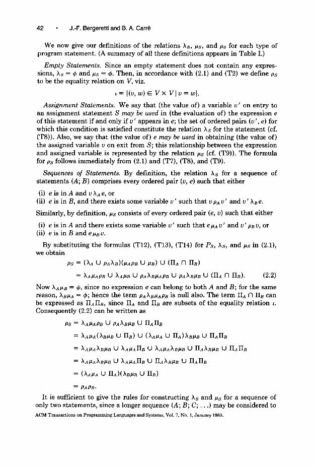
We now give our definitions of the relations Xs, ps, and ps for each type of program statement. (A summary of all these definitions appears in Table I.)
Empty Statements. Since an empty statement does not contain any expres- sions, hs = 4 and PS = 4. Then, in accordance with (2.1) and (T2) we define ps to be the equality relation on V, viz.
l={(U,W)EVXVIU=WJ.
Assignment Statements. We say that (the value of) a variable u’ on entry to an assignment statement S may be used in (the evaluation of) the expression e of this statement if and only if u’ appears in e; the set of ordered pairs (u’, e) for which this condition is satisfied constitute the relation Xs for the statement (cf. (T8)). Also, we say that (the value of) e may be used in obtaining (the value of) the assigned variable u on exit from S; this relationship between the expression and assigned variable is represented by the relation ps (cf. (T9)). The formula for ps follows immediately from (2.1) and (T7), (T8), and (T9).
Sequences of Statements. By definition, the relation Xs for a sequence of statements (A; B) comprises every ordered pair (u, e) such that either
(i) eisinAanduXAe,or (ii) e is in B, and there exists some variable u ’ such that upA u’ and u’ Xge.
Similarly, by definition, ps consists of every ordered pair (e, u) such that either
(i) e is in A and there exists some variable u ’ such that e PA u ’ and u ’ pi u, or (ii) e is in B and e pLg u.
By substituting the formulas (T12), (T13), (T14) for Ps, XS, and ps in (2.1), we obtain
ps = (AA U PAAB)(CLAPB U pi) U (no fl nB)
= AACLAPB U AA/JB U PA~BPAPB U PAABCLB U (no f-l HB). (2.2)
Now XApB = 4, since no expression e can belong to both A and B; for the same reason, hB/.lA = 4; hence the term pAXBpApB is null also. The term IIA n II, can be expressed as &IIB, since IIA and ns are subsets of the equality relation 1. Consequently (2.2) can be written as
Ps = AAPAPB U PA~BPB U HA~B
= PAPB.
It is sufficient to give the rules for constructing Xs and ps for a sequence of only two statements, since a longer sequence (A; B; C; . . .) may be considered to
ACM Transactions on Programming Languages and Systems, Vol. 7, No. 1, January 1985.

Information-Flow and Data-Flow Analysis of while-Programs l 43
be nested, for instance, in the form (((A; B); C); . . .). It is easily verified that the information-flow relations obtained for a sequence of statements (A; B; C; . . .) are independent of the order in which they are combined.
Conditional Statements. Let S be a conditional statement of the form
if e then A else B
Then by definition (the value of) a variable v on entry to S may be used in evaluating an expression e’ (and we have v Xse ‘) if and only if
(i) e’ is the Boolean expression e of the conditional statement and v E I’(e), or (ii) e’ is in A and vXAe’, or
(iii) e ’ is in B and v Xe e ‘.
Similarly, by definition (the value of) an expression e’ may be used in obtaining the value of a variable v on exit from a conditional statement S (and we have e ’ Xs v) if and only if
(i) e’ is the Boolean expression e of S, and either A or B may define v, or (ii) e’ is in A ande’pAv, or
(iii) e’ is in B and e’ ps v.
These definitions are given in symbolic form in (TM) and (T19). From (2.1) and (T17), (T18), (T19),
PS = ((r(e) x (e)) u AA u XB)((k) x @A u DB)) u PA u d u (nA u HB)
= (r(e) x (DA u &3)) u XApA u XBPB u HA u nB
= (r(e) x (DA u DB)) u PA u PB-
A conditional statement S of the form
if e then A
may be regarded as a statement of the form if e then A else B in which B is an empty statement, for which the information-flow relations are given by (Tl)- (T5). Using these, the formulas (T16)-(T20) simplify to (T21HT25).
Repetitive Statements. For a statement S of the form while e do A
the formulas for Xs, p,s, and ps are obtained by assuming that S is equivalent to an infinite sequence of nested conditional statements of the form
if e then begin
A; if e then begin
A;
end end
ACM Transactions on Programming Languages and Systems, Vol. 7, No. 1, January 1985.

44 l J.-F. Bergeretti and 8. A. Car&
To derive the required formulas it will be convenient to use the notations
xe = r(e) X (4, A = (4 X DA, we = I’(e) x DA.
Now by repeated application of (T23) and (T13),
kS = xe u AA u PAhe u AA u PAhe u AA u PA(“‘)))
= (1 u PA u di u pi u ***)(xe u AA)
= p& u AA)
= pX((rk) x (e)) u AA)
where p.$ is the transitive closure of PA. It is convenient next to derive p,$ from (T25) and (T15), whose repeated
applications give
PS = we u 1 u PAbe u 1 u PAb, u L u PA(“‘)))
= (1 u PA u pi u ,,$ u ***)(‘d, u 1)
= PX((r(e) x DA) u 1).
Finally, to obtain PS, we make repeated use of (T24) and (T14), which give
kS = (tie u PAPS) u (i’b u PAPS) * * * = $e u CLAPS
and therefore from (T30) we obtain
1.6 = t(e) X DA) U pAp;((r(e) X DA) U L).
2.3 Construction of the Information-Flow Relations
Given the parse tree of a program generated by the grammar of Figure 1, it is easily possible to compute its information-flow relations by obtaining these for each statement of the program in turn in the course of a post-order traversal [l] of the tree. On visiting a tree node which represents an assignment statement, we obtain its information-flow relations directly from the formulas (T6)-(TlO); on visiting a node which represents a compound, conditional, or repetitive statement S, we use the appropriate formulas of Table I to derive the information- flow relations for S from those of its constituent statements. (These are imme- diate successors of S in the parse tree, which will already have been visited in the post-order traversal.) In this way, at each stage it is only necessary to retain the information-flow relations for the immediate successors of the tree nodes on the path from the tree root to the node currently being visited.
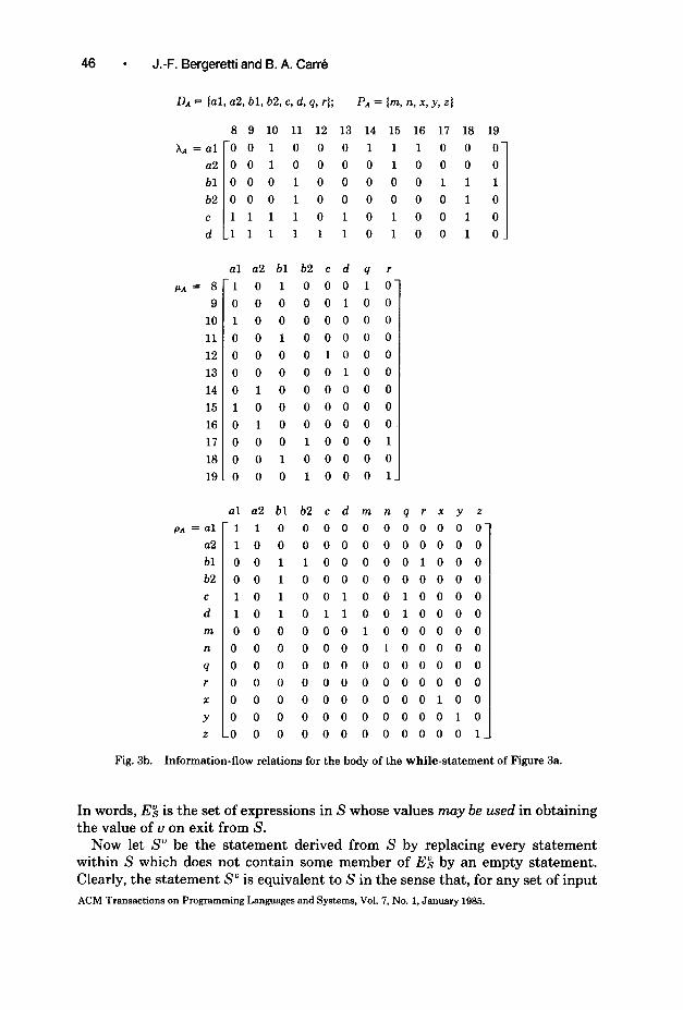
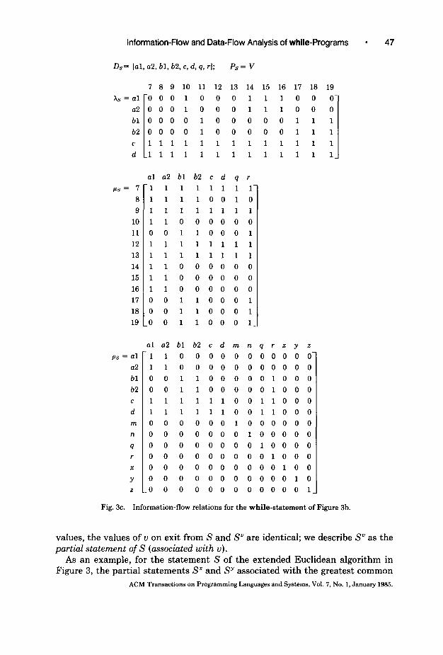
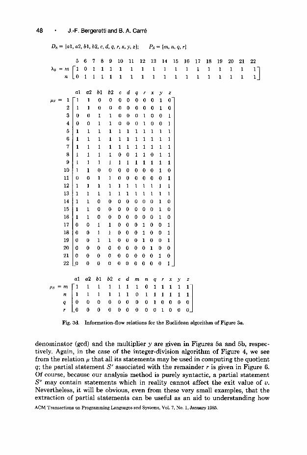
As an example, Figure 3a is the extended Euclidean algorithm, in the form of a Pascal procedure, as presented by Jensen and Wirth [14]. The information- flow relations for the body of its while-statement are given in Figure 3b. (Here each relation is represented by its Boolean relation matrix, with empty rows and columns omitted.) The corresponding relations for the complete while-statement are given in Figure 3c, and those for the entire procedure are shown in Figure 3d. ACM Transactions on Programming Languages and Systems, Vol. 7, No. 1, January 1985.
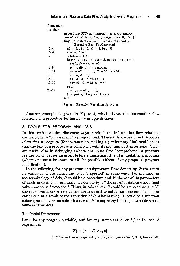
Information-Flow and Data-Flow Analysis of while-Programs l 45
Expression Number
l-4 5,6 7
899 10,ll 12,13 14-16 17-19
20-22
procedure GCD( m, n : integer; var x, y, 2 : integer); var al, a2, bl, b2, c, d, q, r,: integer; {m 2 0, n > 0) begin (Greatest Common Divisor x of m and n,
Extended Euclid’s Algorithm) al := 0; a2 := 1; bl := 1; b2 := 0; c := m; d := n; while d # 0 do begin (al * m + bl * n = d, a2 * m + b2 * n = c,
gcdk, 4 = gcdh n)l q:=cdivd;r:=cmodd; a2 := a2 - q * al; b2 := b2 - q * bl; c := d; d := r; r := al; al := ~2; a2 := r; r := bl; bl := b2; b2 := r
end, x:=c;y:=a2;z:=b2 {n = gcd(m, n) = y * m + .z * n)
end
Fig. 3a. Extended Euclidean algorithm.
Another example is given in Figure 4, which shows the information-flow relations of a procedure for hardware integer division.
3. TOOLS FOR PROGRAM ANALYSIS
In this section we describe some ways in which the information-flow relations can help one to “comprehend” a program text. These aids are useful in the course of writing a program (for instance, in making a preliminary “informal” check that the text of a procedure is consistent with its pre- and post-assertions). They are useful also in debugging (where one must first “comprehend” a program feature which causes an error, before eliminating it), and in updating a program (where one must be aware of all the possible effects of any proposed program modification).
In the following, for any program or subprogram P we denote by Vi the set of its variables whose values are to be “imported” in some way. (For instance, in the terminology of Ada, P could be a procedure and v’ the set of its parameters of mode in or in out). Similarly, we denote by V” the set of variables whose final values are to be “exported.” (Thus, in Ada terms, P could be a procedure and V” the set of variables whose values are assigned to actual parameters of mode in out or out, as a result of the execution of P. Alternatively, P could be a function subprogram, having no side effects, with V” comprising the single variable whose value is returned.)
3.1 Partial Statements
Let u be any program variable, and for any statement S let E,” be the set of expressions
ES = {e E E 1 epsu}.
ACM Transactions on Programming Languages and Systems, Vol. ‘7, No. 1, January 1985.
46 l J.-F. Bergeretti and B. A. Car&
DA = {al, a2, bl, b2, c, d, q, r); PA=lwn,&Y,4
iA = al
a2
bl
b2
c
d
644 = 8 1 0 1 000 10
9 0 0 0 00100
10 1 0 0 0 00 0 0
11 0 0 1 0 00 0 0
12 0 0 0 0 100 0
13 00000100
14 0 1 0 0000 0
15 1 0 0 0000 0
16 010 00000
11 0 0 0 1000 1
18 0 0 1 0 00 0 0
19 -0 0 0 100 0 1
8 9 10 11 12 13 14 15 16 17 18 19
‘0010 0 0 1110 0 0
001000010000
00 0 1 00000111
000 10 0 0 0 0 0 1 0
111101010010
111111 010010
al a2 bl b2 c d q r
al a2 bl b2 c d m n q r x y 2
p‘4=al 1 1 0 0000000000
a2 10 0 0000000000
bl 00 1 100 0 001000
b2 0 o I 0000000000
C 10 1 0010010000
d 10 1 0110010000
m 00 0 0001000000
n 0 0 0 0000100000
4 0000000000000
r 000 0000000000
x 000 0000000100
Y 0 0 0 0000000010
2 -0 0 0 0000000001
Fig. 3b. Information-flow relations for the body of the while-statement of Figure 3a.
In words, E$ is the set of expressions in S whose values may be used in obtaining the value of v on exit from S.
Now let S” be the statement derived from S by replacing every statement within S which does not contain some member of E$ by an empty statement. Clearly, the statement S” is equivalent to S in the sense that, for any set of input ACM Transactions on Programming Languages and Systems, Vol. 7, No. 1, January 1985.
Information-Flow and Data-Flow Analysis of while-Programs 47
Ds= [al, a2, bl, b2, c, d, q. r); Ps= v
7 a 9 10 11 12 13 14
&=a1 0 0 0 1 0 0 0 1
a2 0 0 0 1 0 0 0 1
blOOO0 1 0 0 0
b2 0 0 0 0 1 0 0 0
c 1111 11 11
d-1111 11 11
al a2 bl b2 c d q r ps=7 11 1 1 1 1 1 1.
8 1 1 1 100 10
9 1 1 1 11111
10 1 1 0 00000
11 0 0 1 100 0 1
12 1 1 1 11111
13 1 1 1 11111
14 1 1 0 0000 0
15 1 1 0 0 00 0 0
16 1 1 0 00000
17 0 0 1 100 0 1
18 0 0 1 100 0 1
19,o 0 1 1 0 0 0 1.
al a2 bl b2 c d m n ps = al 1 1 0 0 00 0 0
a2 1 1 0 0 00 0 0
bl 0 0 1 100 0 0
b2 0 0 1 100 0 0
C 1 1 1 11100
d 1 1 1 11100
m 00000010
n 00000001
Q 0 0 0 00000
r 0 0 0 00000
x 0 0 0 00000
Y 0 0 0 0 00 0 0
z -0 0 0 0 00 0 0
15 16 17 18 19
1 1 0 0 0
1 1 0 0 0
0 0 1 1 1
0 0 1 1 1
1 1 1 1 1
1 1 1 1 1
qrxyz 0 0 0 0 0’ 00000 01000
01000
11000
1 10 0 0
00000
00000
10000
0 10 0 0
00100
00010
00001
Fig. 3c. Information-flow relations for the while-statement of Figure 3b.
values, the values of v on exit from S and S” are identical; we describe S” as the partial statement of S (associated with v).
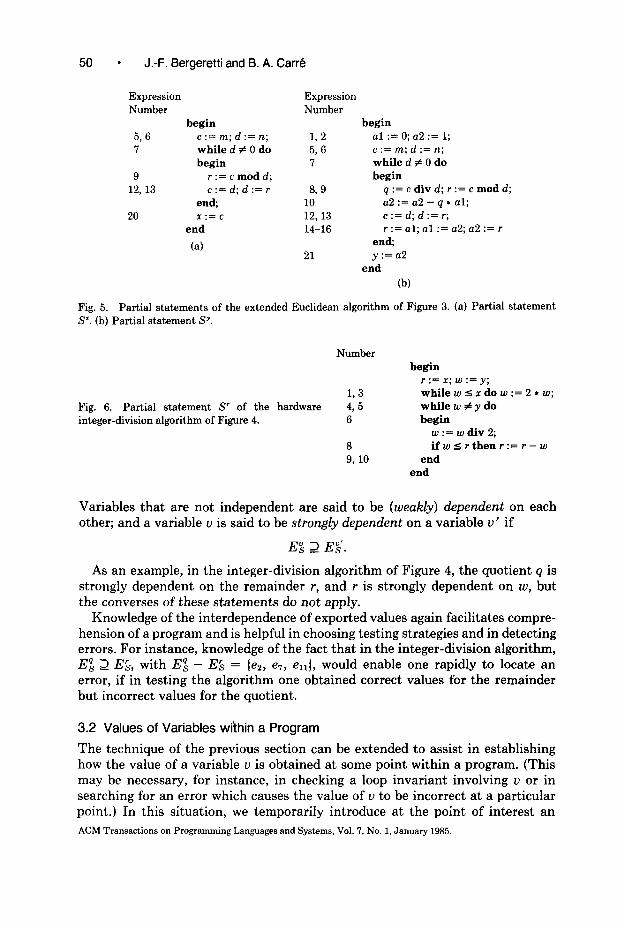
As an example, for the statement S of the extended Euclidean algorithm in Figure 3, the partial statements S” and Sy associated with the greatest common
ACM Transactions on Programming Languages and Systems, Vol. 7, No. 1, January 1985.
48 l J.-F. Bergeretti and B. A. Carrk
DS = lal, a2, 61, b2, c, d, q, r, x, y, zl; PS = Im, n, art
5 6 7 8 9 10 11 12 13 14 15 16 17 18 19 20 21 22
11 1111111111
011111111111111111 1 Irs= 1
2
3
4
5
6
7
8
9
10
11
12
13
14
15
16
17
18
19
20
21
22
PS = m n
9 r
al a2 bl b2 c d q r n y z
1 1 0 00000010‘
1 1 0 00000010
0 0 1 10001001
0 0 1 10001001
1 1 1 11111111
1 1 1 11111111
1 1 1 11111111
1 1 1 10011011
1 1 1 11111111
1 1 0 00000010
0 0 1 10000001
1 1 1 11111111
1 1 1 11111111
1 1 0 00000010
1 1 0 00000010
1 1 0 00000010
0 0 1 10001001
0 0 1 10001001
0 0 1 10001001
0 0 0 00000100
0 0 0 00000010
P 0 0 00000001~
al a2 bl b2 c d m n q r x
-1 1 1 11110111
1 1 1 11101111
0 0 0 00000100
-0 0 0 00000010
Y 2 1 1
1 1
0
0
0 0 I
Fig. 3d. Information-flow relations for the Euclidean algorithm of Figure 3a.
denominator (gcd) and the multiplier y are given in Figures 5a and 5b, respec- tively. Again, in the case of the integer-division algorithm of Figure 4, we see from the relation ~1 that all its statements may be used in computing the quotient q; the partial statement S’ associated with the remainder r is given in Figure 6. Of course, because our analysis method is purely syntactic, a partial statement S” may contain statements which in reality cannot affect the exit value of v. Nevertheless, it will be obvious, even from these very small examples, that the extraction of partial statements can be useful as an aid to understanding how
ACM Transactions on Programming Languages and Systems, Vol. 7, No. 1, January 1985.
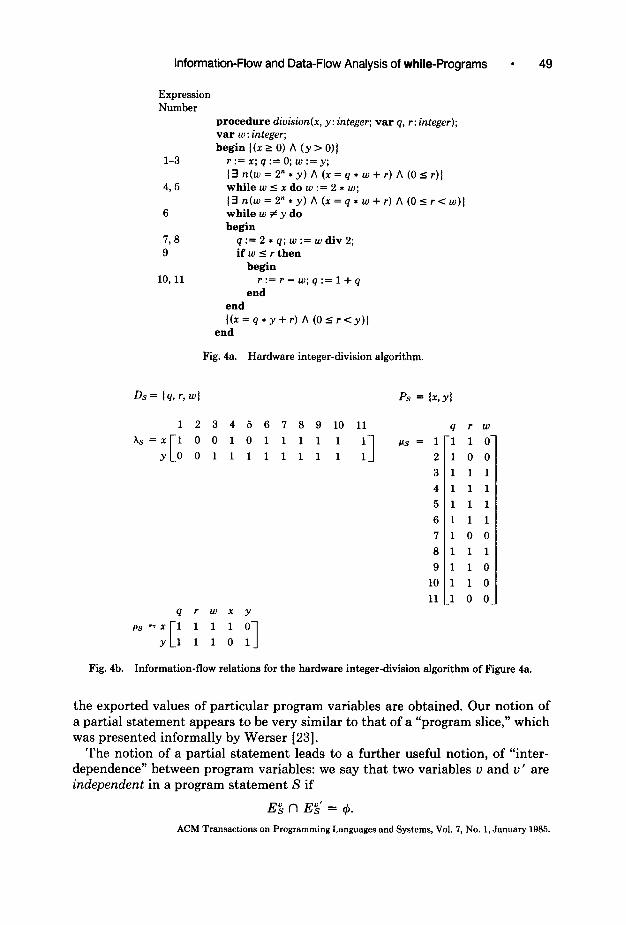
Information-Flow and Data-Flow Analysis of while-Programs . 49
Number procedure diuision(x, y: integer; var q, r: integer);
var w : integer; begin((x?O)A(y>O))
l-3 r := x; q :=o; w:=y;
13n(w=2”*y)A(x=q*w+r)A(O=r))
4,5 while w 5 x do w := 2 * w; {3n(w=2”*y)A(r=q*w+r)A(Osr<w)]
6 while w # y do begin
7, 8 q := 2 * q; w := w div 2; 9 ifwsrthen
begin 10,ll r := r - w; q := 1 + q
end end
en~=q*y+r)A(OsrCY)I
Fig. 4a. Hardware integer-division algorithm.
Ds= Iq,r,wl ps = ISYI
1 2 3 4 5 6 7 8 9 10 11
hs=x10010111111
[ 1 PS = 1 y00111111111 2
3
4
5
6
7
8
9
10
11 qrwxy
ps=x 11
C
11 0
y .l 1 1 0 1 1
q rw 1 1 o-
1 0 0
1 1 1
1 1 1
1 1 1
1 1 1
1 0 0
1 1 1
1 1 0
1 1 0
1 0 o-
Fig. 4b. Information-flow relations for the hardware integer-division algorithm of Figure 4a.
the exported values of particular program variables are obtained. Our notion of a partial statement appears to be very similar to that of a “program slice,” which was presented informally by Werser [23].
The notion of a partial statement leads to a further useful notion, of “inter- dependence” between program variables: we say that two variables u and v ’ are independent in a program statement S if
ACM Transactions on Programming Languages and Systems, Vol. 7, No. 1, January 1985.
50 l J.-F. Bergeretti and B. A. Car&
Expression Number
begin 596 c := m; d := n; 7 while d # 0 do
begin 9 r:=cmodd;
12,13 c := d; d := r end;
20 x := c end
(a)
Expression Number
begin L2 al := 0; a2 := 1; 5,6 c := m; d := n; 7 while d # 0 do
begin 89 q := c div d; r := c mod d;
10 a2 := a2 - q * al; 12,13 c := d; d := r; 14-16 I-:= al; al := a2; a2 := r
end; 21 y:=a2
end
(b)
Fig. 5. Partial statements of the extended Euclidean algorithm of Figure 3. (a) Partial statement S”. (b) Partial statement Sy.
Number begin
r:=x;w:=y; 193 whilewsxdow:=2*w;
Fig. 6. Partial statement S’ of the hardware 4, 5 while w # y do integer-division algorithm of Figure 4. 6 begin
w:=wdiv2; 8 ifwsrthenr:=r-w 9, 10 end
end
Variables that are not independent are said to be (weakly) dependent on each other; and a variable v is said to be strongly dependent on a variable v’ if
As an example, in the integer-division algorithm of Figure 4, the quotient q is strongly dependent on the remainder F, and r is strongly dependent on w, but the converses of these statements do not apply.
Knowledge of the interdependence of exported values again facilitates compre- hension of a program and is helpful in choosing testing strategies and in detecting errors. For instance, knowledge of the fact that in the integer-division algorithm, Ez 2 E&, with Ei - Eb = (ez, e7, ellJ, would enable one rapidly to locate an error, if in testing the algorithm one obtained correct values for the remainder but incorrect values for the quotient.
3.2 Values of Variables within a Program
The technique of the previous section can be extended to assist in establishing how the value of a variable v is obtained at some point within a program. (This may be necessary, for instance, in checking a loop invariant involving v or in searching for an error which causes the value of v to be incorrect at a particular point.) In this situation, we temporarily introduce at the point of interest an ACM Transactions on Programming Languages and Systems, Vol. 7, No. 1, January 1985.
Information-Flow and Data-Flow Analysis of while-Programs l 51
assignment u ’ := u to a new variable u’; the relevant statements are then all contained in the partial statement associated with u’.
3.3 Information Propagation within a Program
In analyzing a program, for instance to update it, one often wishes to know all the possible ways in which the value of some variable u at a particular point within the program may affect the subsequent program execution. (This problem arises, for instance, if one envisages inserting or modifying a particular assign- ment to u.)
To solve this problem, we may temporarily introduce a new program variable U’ and insert at the point of interest an assignment statement u := v’. Then, in the statement part S of the program, the set of all expressions whose evaluations may employ the value of u at x (assuming that all program paths are executable) is
(eEE)u’Xse)
and the set of variables for which the computation of exit values may employ the value of v at x (assuming that all paths are executable) is
(u E VI u’psu).
3.4 Input-Output Relations
For any program or subprogram P, the p-relation indicates those members of v’ whose values on entry to P may be used in obtaining the value, on exit from P, of each member of V”. Thus a tabulation of p provides a useful indication of whether the relationships between input and output values are as required. As will be explained below, the evaluation of p for a procedure P also makes it possible to perform the type of analysis described here for a program in which P is embedded.
4. AUTOMATIC DETECTION OF ERRORS AND ANOMALIES
In this section we first describe a number of tests that can be performed on the X-, p-, and p-relations of a program to reveal particular kinds of programming errors. We then relate these tests to the well-known techniques of data-flow analysis.
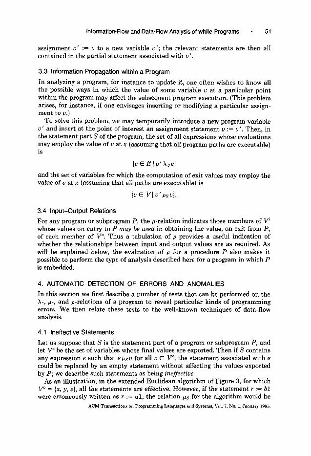
4.1 Ineffective Statements
Let us suppose that S is the statement part of a program or subprogram P, and let V” be the set of variables whose final values are exported. Then if S contains any expression e such that e Es u for all u E V”, the statement associated with e could be replaced by an empty statement without affecting the values exported by P; we describe such statements as being ineffective.
As an illustration, in the extended Euclidean algorithm of Figure 3, for which V” = (x, y, z), all the statements are effective. However, if the statement r := bl were erroneously written as r := al, the relation ks for the algorithm would be
ACM Transactions on Programming Languages and Systems, Vol. 7, No. 1, January 1985.
52 l J.-F. Bergeretti and B. A. Carri!
IQ= 1 2
3
4
5
6
7
8
9
10
11
12
13
14
15
16
17
18
19
20
21
22
al a2 bl b2 c d q r XY 2
1 1 1 10000 0 1 1.
1 1 1 10000 0 1 1
0 0 1 00000 0 0 0
0 0 1 10000 0 0 1
1 1 1 1 1 1 1 1 1 1 1
1 1 1 11111 1 1 1
1 1 1 1 1 1 1 1 1 1 1
1 1 1 10011 0 1 1
1 1 1 1 1 1 1 1 1 1 1
1 1 1 10001 0 1 1
0 0 1 00000 0 0 0
1 1 1 11111 1 1 1
1 1 1 11111 1 1 1
1 1 1 10001 0 1 1
1 1 1 10001 0 1 1
1 1 1 10001 0 1 1
0 0 1 10001 0 0 1
0 0 1 00000 0 0 0
0 0 1 10000 0 0 1
0 0 0 00000 1 0 0
00 0 00000 0 1 0
0 0 0 00000 0 0 1
Fig. 7. p-relation for modified Euclidean algorithm.
that shown in Figure 7, which indicates that the statements 3, 11, and 18 are ineffective.
4.2 Ineffective Imported Values
Let P be a subprogram with specified sets Vi and V” of imported and exported variables, respectively. If for any variable u E v’ we have u js u ’ for all u ’ E V”, then the imported value of u cannot be used in the evaluation of any exported value; we describe such an imported value u as being ineffectiue.
4.3 Undefined Variables
Let S be the statement part of a program or subprogram P, and let Vi be the set of variables for which initial values are to be imported by P.
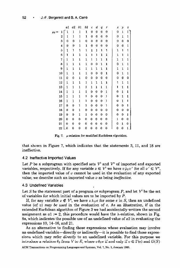
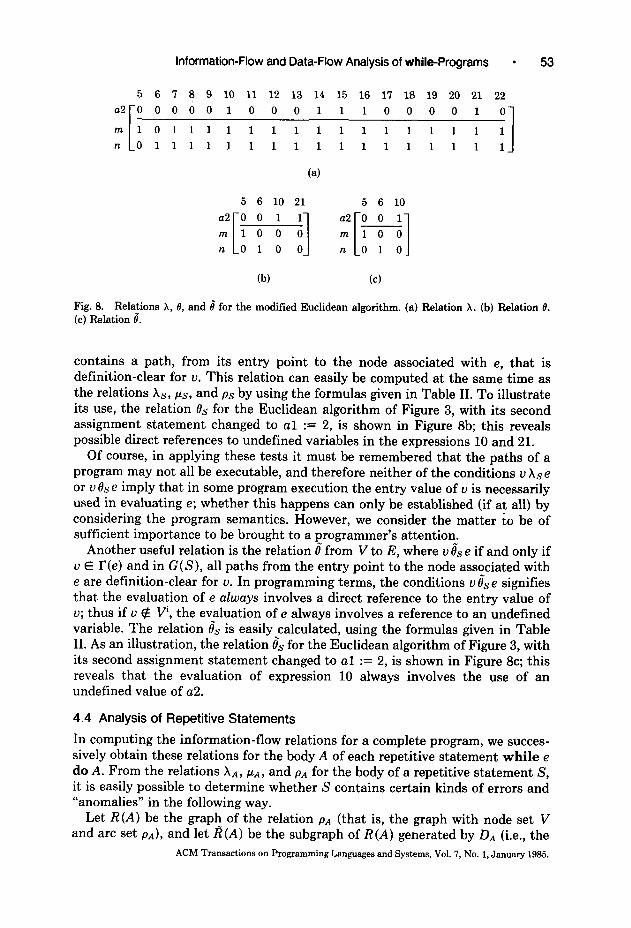
If, for any variable u 4 v’, we have u Xae for some e in S, then an undefined value (of u) may be used in the evaluation of e. As an illustration, if in the extended Euclidean algorithm of Figure 3 we had accidentally plritten the second assignment as al := 2, this procedure would have the X-relation, shown in Fig. Ba, which indicates the possible use of an undefined value of a2 in evaluating the expressions 10, 14-16, and 21.
As an alternative to finding those expressions whose evaluation may involve an undefined variable-directly or indirectly-it is possible to find those expres- sions which may refer directly to an undefined variable. For this purpose we introduce a relation Bs from V to E, where u&e if and only if u E I’(e) and G(S)
ACM Transactions on Programming Languages and Systems, Vol. 7, No. 1, January 1985.
Information-Flow and Data-Flow Analysis of while-Programs l 53
5 6 7 8 9 10 11 12 13 14 15 16 17 18 19 20 21 22
000010
011111111111111111 I
(a)
5 6 10 21 5 6 10
(b) (c)
Fig. 8. Relations X, 19, and e” for the modified Euclidean algorithm. (a) Relation X. (b) Relation 0. (c) Relation e’.
contains a path, from its entry point to the node associated with e, that is definition-clear for u. This relation can easily be computed at the same time as the relations XS, PS, and ps by using the formulas given in Table II. To illustrate its use, the relation 0,s for the Euclidean algorithm of Figure 3, with its second assignment statement changed to al := 2, is shown in Figure 8b; this reveals possible direct references to undefined variables in the expressions 10 and 21.
Of course, in applying these tests it must be remembered that the paths of a program may not all be executable, and therefore neither of the conditions v hs e or u 0s e imply that in some program execution the entry value of u is necessarily used in evaluating e; whether this happens can only be established (if at all) by considering the program semantics. However, we consider the matter to be of sufficient importance to be brought to a programmer’s attention.
Another useful relation is the relation 8 from V to E, where u 8s e if and only if u E r(e) and in G(S), all paths from the entry point to the node associated with e are definition-clear for u. In programming terms, the conditions IJ 8,s e signifies that the evaluation of e always involves a direct reference to the entry value of v; thus if u 4 Vi, the evaluation of e always involves a reference to an undefined variable. The relation & is easily calculated, using the formulas given in Table II. As an illustration, the relation & for the Euclidean algorithm of Figure 3, with its second assignment statement changed to al := 2, is shown in Figure 8c; this reveals that the evaluation of expression 10 always involves the use of an undefined value of a2.
4.4 Analysis of Repetitive Statements
In computing the information-flow relations for a complete program, we succes- sively obtain these relations for the body A of each repetitive statement while e do A. From the relations XA, PA, and PA for the body of a repetitive statement S, it is easily possible to determine whether S contains certain kinds of errors and “anomalies” in the following way.
Let R(A) be the graph of the relation PA (that is, the graph with node set V and arc set PA), and let R(A) be the subgraph of R(A) generated by DA (i.e., the
ACM Transactions on Programming Languages and Systems, Vol. 7, No. 1, January 1985.

54 ’ J.-F. Bergeretti and B. A. Carri!
Table II. Expressions for the Relations 0s and &
Empty Statements. For an empty (or “skip”) statement S,
&s = 6; 8s = 4.
Assignment Statements. For an assignment statement S, which assigns a value to u and whose (expression) part is e,
OS = r(e) X (e); & = r(e) X [ej.
Sequences of Statements. For a sequence S of two statements (A; B), 0.9 = 0~ U {(u, e) E 0~1~ EPA]; c = 8A u ((u, e) E & 1 u 4 DA].
Conditional Statements. For a statement S of the form: if e then A else B
19s = (r(e) X {e)) U 19, U 0~; & = (r(e) X (e)) U 8, U &.
For a statement S of the form: if e then A
OS = (r(e) x iel) u 0.4 i, = (r(e) x [e)) u fYA.
Repetitiue Statements. For a statement S of the form: while e do A
8~ = 0%) x 14) u 0~; h= ke’) E ((r(e) x 14) U iLA)Iu4D.44.
graph with node set DA and arc set pA n (DA X DA)). A variable v E DA is said to be stable (with respect to S) if on a(A) there is no path to v from any variable which lies on a cycle. The stability index as(v) of a variable v which is stable in S is defined as the length (i.e., the number of arcs) of a longest path on R(A) which terminates on v.
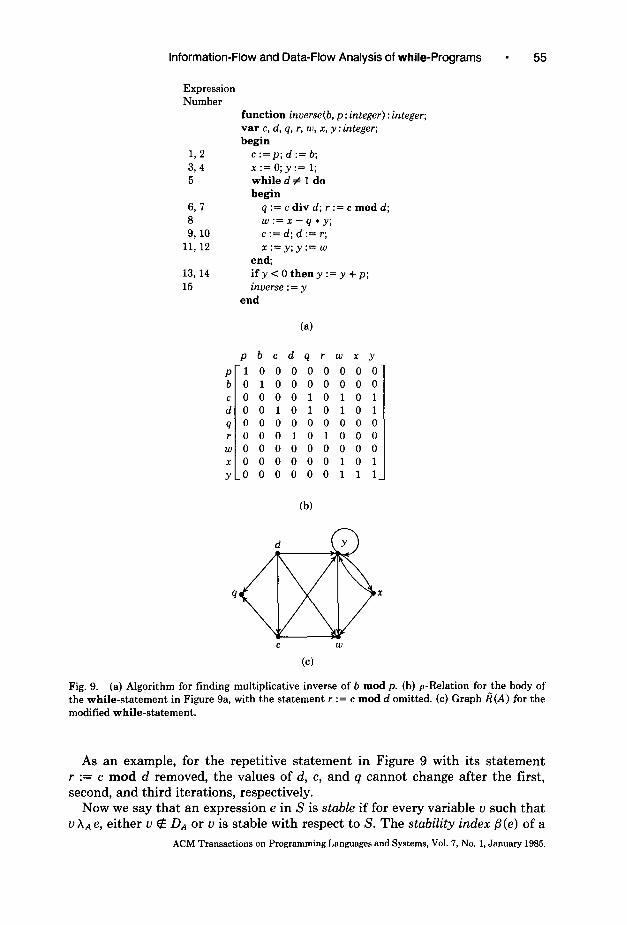
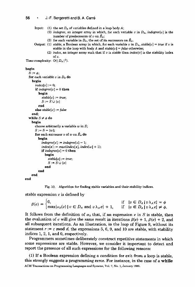
As an example, in the repetitive statement of the algorithm given in Figure 9a, none of the variables are stable. However, if the statement r := c mod d is omitted, the relation PA for the loop body becomes that shown in Figure 9b, and the corresponding graph fi(A) is that of Figure 9c; from this graph we see that the variables d, c, and q are stable, with stability indices 0, 1, and 2, respectively. (Stable nodes, with their indices, can easily be determined using the algorithm of Figure 10, which is a modified form of the algorithm commonly employed for finding node rank in acyclic graphs [5].)
In programming terms, the notion of stability has the following significance. Let us suppose that for some set of input values to S, some number h > 0 of iterations are performed, and for each variable v E V, let us denote by v@) the value of v after the kth execution of A. Now the value of any variable v which does not belong to DA cannot be modified in the execution of A. Alternatively, if u E DA, then A contains an assignment to v, but in this case if as(v) = 0 then IJ ’ jA v for all u ’ E DA, which implies that
v(k+l) = vW f for k = 1, 2, . . . , h - 1.
If v 4 DA and as(u) = 1, then for any variable v ’ such that u ’ PA u, either v ’ E Da or a(v ‘) = 0, which implies that
v(k+l) = v(k) , for k = 2,3, . . . , h - 1.
By extension of this argument we find that for any stable variable v, u(k+l) = u(k)
, for k = as(v) + 1, C&V) + 2, . . . , h - 1. ACM Transactions on Programming Languages and Systems, Vol. ‘7, No. 1, January 1985.
Information-Flow and Data-Flow Analysis of while-Programs 55
Expression Number
function inverse(b, p: integer) : integer; var c, d, q, r, w, n, y : integer; begin
L2 c :=p; d := b;
3,4 r:=O;y:= 1; 5 while d # 1 do
begin
6, 7 q := c div d; r := c mod d; 8 w:=x-q*y; 9,lO c := d; d := r;
11,12 r:=y;y:= w
end; 13,14 ify<Otheny:=y+p; 15 inverse : = y
end
pbcdqrwxy
p100000000 b010000000 c000010101 d001010101 qooooooooo r000101000
wooooooooo x000000101 y-0 0 0 0 0 0 111
(b)
d Y
9 clxi!5 X
C W
(cl
Fig. 9. (a) Algorithm for finding multiplicative inverse of b mod p. (b) p-Relation for the body of the while-statement in Figure 9a, with the statement r := c mod d omitted. (c) Graph I?(A) for the modified while-statement.
As an example, for the repetitive statement in Figure 9 with its statement r := c mod d removed, the values of d, c, and q cannot change after the first, second, and third iterations, respectively.
Now we say that an expression e in S is stable if for every variable v such that v XA e, either v 4 DA or v is stable with respect to S. The stability index /l(e) of a
ACM Transactions on Programming Languages and Systems, Vol. 7, No. 1, January 1985.
56 l J.-F. Bergeretti and B. A. Cart%
Input: (1) the set DA of variables defined in a loop body A; (2) indegree, an integer array in which, for each variable u in DA, idegree[u] is the
number of predecessors of u on I?,,; (3) for each variable in DA, the set of its successors on I&.
Output: (1) stable, a Boolean array in which, for each variable u in DA, stab.!e[u] = true if u is stable in the loop with body A and stabk[u] = fake otherwise;
(2) index, an integer array such that if u is stable then index[u] is the stability index of u.
Time complexity: 0( 1 DA 1’).
begin s := l#l; for each variable u in DA do
begin irdex[u] := 0; if indegree[u] = 0 then
begin stable[u] := true; s := s lJ {u)
end else stabk[u] := fake
end, while S # 4 do
begin choose arbitrarily a variable w in S; s := s - (w); for each successor r of w on k,, do
begin indegree[x] := idegree[x] - 1; index[x] := max(index[x], index[w] + 1); if indegree[x] = 0 then
begin stub&] := true; s := s u {x)
end end
end end
Fig. 10. Algorithm for finding stable variables and their stability indices.
stable expression e is defined by
P(e) = iax{c&U) 1 u E DA and u XAe) + 1, if (u E DA 1 uXAeJ if (uEDAIuXAe}
It follows from the definition of as that, if an expression e in S is stable, then the evaluation of e will give the same result in iterations P(e) + 1, /3(e) f 2, and all subsequent iterations. As an illustration, in the loop of Figure 9, without its statement F := c mod d, the expressions 5, 6, 9, and 10 are stable, with stability indices 1, 2, 1, and 0, respectively.
Programmers sometimes deliberately construct repetitive statements in which some expressions are stable. However, we consider it important to detect and report the presence of all such expressions for the following reasons:
(1) If a Boolean expression defining a condition for exit from a loop is stable, this strongly suggests a programming error. For instance, in the case of a while ACM Transactions on Programming Languages and Systems, Vol. 7, No. 1, January 1985.
information-Flow and Data-Flow Analysis of while-Programs 57
e do A statement, the stability of e implies that in any program execution at most /3(e) iterations can be performed, if the execution of the statement is to terminate. In particular, if /3(e) = 0 the program certainly contains an error, and if P(e) = 1 then either the program contains an error or the repetitive statement could be replaced by if e then A. Even if /3(e) > 1, the stability of e warrants attention, because some very common programming errors such as the omission of statements or misnaming of variables frequently manifest themselves in this way.
(2) The stability of one or more expressions within A suggests that either the repetitive statement S contains an error or that one or more statements could possibly be “hoisted” out of S. Such a modification often makes a program more comprehensible (and possibly more efficient). The detection and “hoisting” of assignment statements whose (expression) parts are stable of index 0 is well known in the context of optimizing compilers [2]. The techniques described here immediately reveal all the statements which could be treated in this way.
4.5 A Comparison with Data-Flow Analysis
The information given by the I%, X-, and p-relations is somewhat similar in nature to that obtained by global data-flow analysis [3, 10-12, 15,161. Furthermore, our strategy for constructing flow relations, in traversing a parse tree, bears some resemblance to the data-flow methods based on graph grammars [8] and “high- level dataflow analysis” [20]. It is therefore instructive to relate these methods and, in particular, to compare the capabilities of our error-detection techniques with those based on data-flow analysis [9, 10, 131.
First, the relations e” and 0 are easily interpreted in terms of “reaching definitions,” as presented, for instance, by Hecht [12] and Kennedy [15]. Let us suppose that at the entry point of a program, we have an initial definition of each of its variables (with any variable which does not belong to v’ being assigned an “undefined value”). Then the condition ve”e signifies that the variable v appears in e, the initial definition of v reaches the statement whose (expression) part is e, and no other definition of v reaches that statement; whereas the condition v 0 e signifies that v appears in e and the initial definition of v reaches the statement with (expression) part e. Thus the relations 0 and e” indicate the “upward-exposed uses” of program variables; or in the terminology of Fosdick and Osterweil [9], for each variable v 4 v’ the condition v 0 e reveals a data-flow error in evaluating e, while the condition v e”e indicates a “significant” data-flow error.
The X-relation is more difficult to interpret, because it provides information not obtainable by data-flow analysis, but we can view it as describing the “propagation” of upward-exposed uses of variables. (As an illustration, in our example of Section 4.3, whose relations are given in Figure 8, the X-relation indicates that the initial (undefined) value of a2 may be used in evaluating the expressions 14, 15_, and 16; these would all be indirect uses of the initial value of a2.) In fact, the 8- and &relations are more useful for detecting references to undefined variables than the X-relation, whose purpose is primarily to study information propagation in the manner described in Section 3.3.
The technique for finding ineffective statements from the p-relation (described in Section 4.1) can be compared with methods of detecting “dead code,” based on a live-variable analysis [ 12, 151. The method based on the p-relation is simpler
ACM Transactions on Programming Languages and Systems, Vol. 7, No. 1, January 1985.
58 l J.-F. Bergeretti and 8. A. Carri!
and more effective, because the p-relation indicates directly all those statements (including conditional and repetitive statements) whose execution cannot affect the final values of any variables which are live on exit.
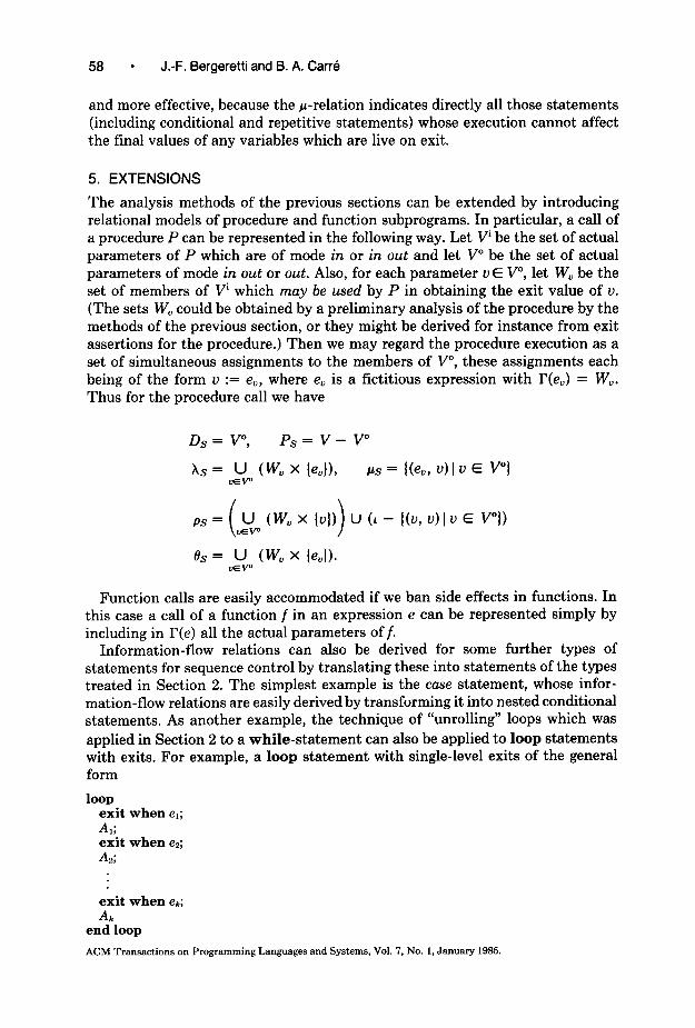
5. EXTENSIONS
The analysis methods of the previous sections can be extended by introducing relational models of procedure and function subprograms. In particular, a call of a procedure P can be represented in the following way. Let Vi be the set of actual parameters of P which are of mode in or in out and let V” be the set of actual parameters of mode in out or out. Also, for each parameter uE V”, let W, be the set of members of v’ which may be used by P in obtaining the exit value of u. (The sets W, could be obtained by a preliminary analysis of the procedure by the methods of the previous section, or they might be derived for instance from exit assertions for the procedure.) Then we may regard the procedure execution as a set of simultaneous assignments to the members of V”, these assignments each being of the form u := e,, where e, is a fictitious expression with I’(e,) = W,. Thus for the procedure call we have
Ds = V”, Ps = v - V”
AS = “pp (WV X IeJ), PS = I@,, 4 I u E W
Function calls are easily accommodated if we ban side effects in functions. In this case a call of a function f in an expression e can be represented simply by including in I’(e) all the actual parameters off.
Information-flow relations can also be derived for some further types of statements for sequence control by translating these into statements of the types treated in Section 2. The simplest example is the case statement, whose infor- mation-flow relations are easily derived by transforming it into nested conditional statements, As another example, the technique of “unrolling” loops which was applied in Section 2 to a while-statement can also be applied to loop statements with exits. For example, a loop statement with single-level exits of the general form
loop . exit when e,; AI; exit when e2; AZ;
exit when ek; Ak
end loop
ACM Transactions on Programming Languages and Systems, Vol. 7, No. 1, January 1985.
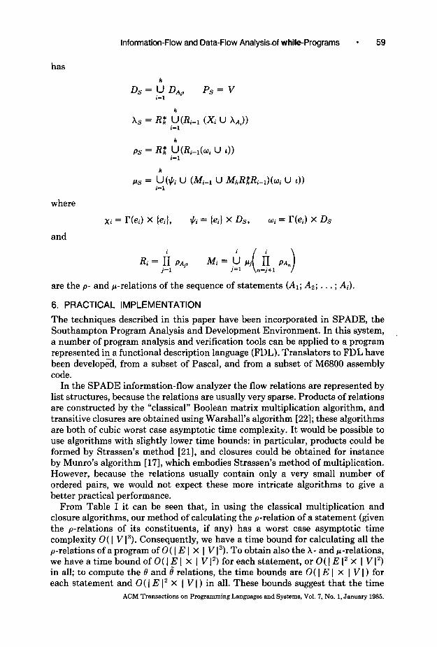
Information-Flow and Data-Flow Analysisof while-Programs 59
has
Ds = If; D.+, Ps = v i=l
PS = Rk* i!l(Ri-,(wi U ~1)
where
Xi = r(G) X lei), $i = leil x Ds, oi = I’(ei) x Ds
and
Ri = i PAj, j=l
are the p- and p-relations of the sequence of statements (Al; A,; . . . ; Ai).
6. PRACTICAL IMPLEMENTATION
The techniques described in this paper have been incorporated in SPADE, the Southampton Program Analysis and Development Environment. In this system, a number of program analysis and verification tools can be applied to a program represented in a functional description language (FDL). Translators to FDL have been develop&l, from a subset of Pascal, and from a subset of M6800 assembly code.
In the SPADE information-flow analyzer the flow relations are represented by list structures, because the relations are usually very sparse. Products of relations are constructed by the “classical” Boolean matrix multiplication algorithm, and transitive closures are obtained using Warshall’s algorithm [22]; these algorithms are both of cubic worst case asymptotic time complexity, It would be possible to use algorithms with slightly lower time bounds: in particular, products could be formed by Strassen’s method [21], and closures could be obtained for instance by Munro’s algorithm [ 171, which embodies Strassen’s method of multiplication. However, because the relations usually contain only a very small number of ordered pairs, we would not expect these more intricate algorithms to give a better practical performance.
From Table I it can be seen that, in using the classical multiplication and closure algorithms, our method of calculating the p-relation of a statement (given the p-relations of its constituents, if any) has a worst case asymptotic time complexity 0( ] V 13). Consequently, we have a time bound for calculating all the p-relations of a program of 0( ] E ] X ] V 13). To obtain also the X- and p-relations, wehaveatimeboundofO(]E( x ]V]2)foreachstatement,orO(]E(2~ IVl”) in all; to compute the 0 and 8 relations, the time bounds are 0( ] E I x I VI ) for each statement and O( ] E I2 x ] VI) in all. These bounds suggest that the time
ACM Transactions on Programming Languages and Systems, Vol. 7, No. 1, January 1985.

60 l J.-F. Bergeretti and B. A. Carr6
requirements could be severe, but in practice, because the relations are extremely sparse, the running times have been found to be quite acceptable: for instance, in a Pascal implementation on a PDP-11/44, the information-flow analysis of the covariance procedure 2 of Witten [24], which has 14 variables and 50 statements, of which 15 are for-statements requiring closure computations, took 8 seconds.
With regard to space complexity, in the worst case the space required to store a single p-relation is of order 0( ] V I’), and therefore (in the worst case) the total space required in computing the p-relation for a program is 0( ] E ] x ] V 12). To compute as well the X-, p-, and e-relations the additional space requirements, in the worst case, are of order O( ] E I2 X V). Again, in practice the space require- ments have been found to be much less severe than these bounds would suggest, partly because the relations are very sparse, and also because in following the procedure described in Section 2.3, the number of relations which need to be retained in analyzing a complete program is relatively small.
The information-flow analyzer is provided with specifications of the sets V’ and V” of variables whose values are imported and exported by a program or subprogram. (These can be passed to it, for instance, via “annotations” of a Pascal text.) This allows the analyzer to detect from the computed relations all errors of the kinds discussed in Section 4, which are signaled to the SPADE user. Stability tests on each repetitive statement are performed at the time when its p-relation is constructed.
7. CONCLUSIONS
The calculation of the information-flow relations is feasible, in polynomial time and space, for an important class of programs. Although the analysis is purely syntactic, with the underlying assumption that all program paths are executable, the methods of extracting partial statements and of finding statements that may affect or may be affected by particular variable values within a program can greatly assist one’s comprehension of its action. These methods are currently being incorporated in a program development environment, in which it will be possible to use the p- and X-relations to determine which program statements are to be displayed by a text editor. The p-relation also provides a useful indication of whether the relationship between input and output variables is as required.
With regard to automatic error detection, the tests for ineffectiveness of statements and variables and for loop stability are easy to perform and usefully extend the class of errors and anomalies which can be detected by static analysis.
ACKNOWLEDGMENTS
The authors are indebted to Dr. B. D. Bramson, Dr. W. J. Cullyer, and S. J. Goodenough of the Royal Signals and Radar Establishment, Malvern, for helpful discussions.
REFERENCES
1. AHO, A.V., HOPCROFT, J.E., AND ULLMAN, J.D. The Design and Analysis of Computer Algo- rithms. Addison-Wesley, Reading, Mass., 1974.
2. AHO, A.V., AND ULLMAN, J.D. The Theory of Parsing, Translation and Compiling, Vol. 2: Compiling. Prentice-Hall, Englewood Cliffs, N.J., 1973.
ACM Transactions on Programming Languages and Systems, Vol. 7, No. 1, January 1985.
Information-Flow and Data-Flow Analysis of while-Programs 61
3. ALLEN, F.E., AND COCKE, J. A program data flow analysis procedure. Commun. ACM 19, 3 (Mar. 1976), 137-147.
4. ANDREWS, G.R., AND REITMAN, R.P. An axiomatic approach to information flow in programs. ACM Trans. Prog. Lang. Syst. 2, 1 (Jan. 1980), 56-76.
5. CARRE, B.A. Graphs and Networks. Oxford University Press, New York, 1979. 6. COHEN, E. Information transmission in sequential programs. In Foundations of Secure Com-
putation, R. A. Demillo et al., Ed. Academic Press, New York, 1978, pp. 297-335. 7. DENNING, D.E., AND DENNING, P.J. Certification of programs for secure information flow.
Commun. ACM 20,7 (July 1977), 504-513. 8. FARROW, R., KENNEDY, K., AND ZUCCONI, L. Graph grammars and global program flow
analysis. In Proceedings of the 17th Annual IEEE Symposium on Foundations of Computer Science (Houston, Tex., Nov.). IEEE, New York, 1975, pp. 42-56.
9. FOSDICK L.D., AND OSTERWEIL, L.J. Validation and global optimization of programs. In Proceedings of the 4th Texas Conference on Computing Systems (Austin, Tex.). 1975. Sponsored by the IEEE Computer Society.
10. FOSDICK, L.D., AND OSTERWEIL, L.J. Data flow analysis in software reliability. ACM Comput. Suru. 8, 3 (Sept. 1976), 305-330.
11. GRAHAM,, S.L., AND WEGMAN, M. A fast and usually linear algorithm for global flow analysis. J. ACM 23, 1 (Sept. 1976), 172-202.
12. HECHT, M.S. Flow Analysis of Computer Programs. Elsevier North-Holland, New York, 1977. 13. HUANG, J.C. Detection of data flow anomaly through program instrumentation. IEEE Trans.
Softw. Eng. SE-&3 (May 1979), 226-236. 14. JENSEN, K., AND WIRTH, N. PASCAL User Manual and Report, 2nd ed. Springer-Verlag, New
York, 1974. 15. KENNEDY, K. A survey of data flow analysis techniques. In Program Flaw Analysis: Theory and
Applications, S. S. Muchnick and N. D. Jones, Eds. Prentice-Hall, Englewood Cliffs, N.J., 1981, pp. 5-54.
16. KILDALL, G.A. A unified approach to global program optimization. In Conference Record of the ACM Symposium on Principles of Programming Languages (Boston, Mass., Oct.). ACM, New York, 1973, pp. 194-206.
17. MUNRO, I. Efficient determination of the transitive closure of a directed graph. Znf. Process. L&t. 1 (1971), 56-58.
18. OSTERWEIL, L.J. Using data flow tools in software engineering. In Program Flaw Analysis: Theory and Applications, S. S. Muchnick and N. D. Jones, Eds. Prentice-Hall, Englewood Cliffs, N.J., 1981, pp. 237-263.
19. POPEK, G.J., HORNING, J.J., LAMPSON, B.W., MITCHELL, W.G., AND LONDON, R.L. Notes on the Design of EUCLID. In SIGPLAN Not. 12,3 (Mar. 1977), 11-18.
20. ROSEN, B.K. High level data flow analysis. Commun. ACM 20,lO (Oct. 1977), 712-724. 21. STRASSEN, V. Gaussian elimination is not optimal. Numer. Math. 13 (1969). 22. WARSHALL, S. A theorem on Boolean matrices. J. ACM 9, 1 (Jan. 1962), 11-13. 23. WERSER, M. Programmers use slicing when debugging. Commun. ACM 25,7 (July 1982), 446-
452. 24. WITTEN, I.H. Algorithms for adaptive linear prediction. Comput. J. 23, 1 (Feb. 1980), 78-84.
Received April 1982; revised August 1983 and July 1984; accepted July 1984
ACM Transactions on Programming Languages and Systems, Vol. 7, No. 1, January 1985.