information frictions in securitization markets: investor
TRANSCRIPT

Information Frictions in Securitization Markets:
Investor Sophistication or Asset Opacity?
David Echeverry ∗
December 8, 2017
Abstract
The performance of a security backed by a pool of loans is affected by default correlation,and not only the probability of default. I imply default correlation from the market priceof collateralized mortgage obligations. Implied correlations are informative about subsequentbond downgrades, but this information content depends on the quality of documentation onthe underlying loans. Correlations implied from junior tranches are no more informative thanthose of AAA tranches for “low-doc deals, and the latter no less informative than the formerfor “full-doc deals. Errors in computing default correlations were thus not driven by AAAinvestors but rather by “low-doc” investors.
JEL classification: G21, G24
Keywords: credit rating agencies, mortgages, securitization, mortgage-backed securities, valuation, com-
peting risks.
∗Haas School of Business. Email:david [email protected]. I thank Martijn Cremers, Nicolae
Garleanu, Amir Kermani, Joseph Kaboski, Ilenin Kondo, Haoyang Liu, Christopher Palmer and Nancy Wallace
for their helpful comments and suggestions, as well as seminar participants at Universidad de los Andes and Uni-
versity of Notre Dame.
1
Because the central premise of securitization is diversification through pooling, default correlations
are crucial to bondholders. Hence prices of structured products that are subject to default risk
reveal investors’ beliefs about correlations. Higher correlations imply more volatility of the portfolio
cashflows, which is valuable to subordinate bondholders but detrimental to senior ones (Duffie and
Garleanu, 2001). Yet there is still a lack of attention to default correlations -which Duffie (2008)
deems the “weak link” in the pricing of collateralized debt obligations (CDO)- relative to the
attention given to default probabilities.
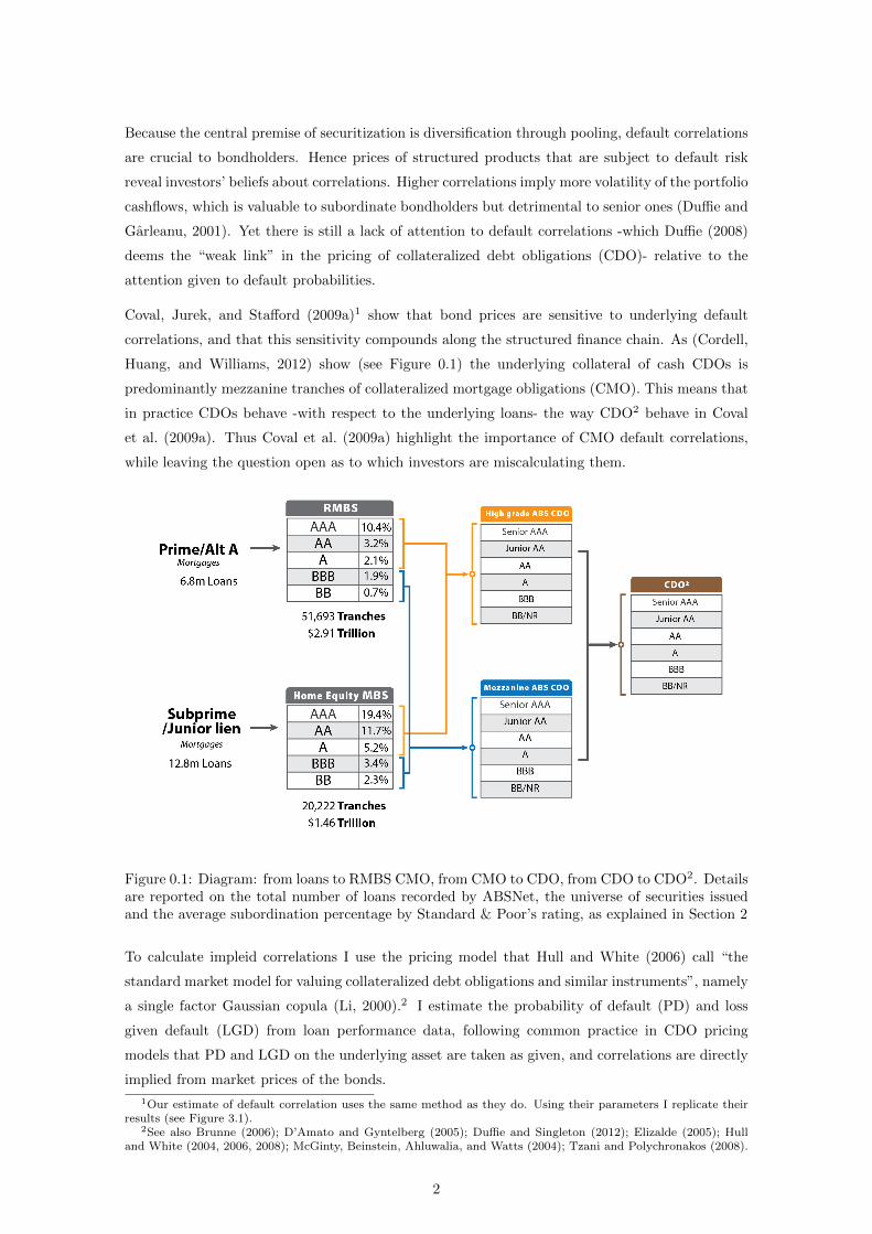
Coval, Jurek, and Stafford (2009a)1 show that bond prices are sensitive to underlying default
correlations, and that this sensitivity compounds along the structured finance chain. As (Cordell,
Huang, and Williams, 2012) show (see Figure 0.1) the underlying collateral of cash CDOs is
predominantly mezzanine tranches of collateralized mortgage obligations (CMO). This means that
in practice CDOs behave -with respect to the underlying loans- the way CDO2 behave in Coval
et al. (2009a). Thus Coval et al. (2009a) highlight the importance of CMO default correlations,
while leaving the question open as to which investors are miscalculating them.
Figure 0.1: Diagram: from loans to RMBS CMO, from CMO to CDO, from CDO to CDO2. Detailsare reported on the total number of loans recorded by ABSNet, the universe of securities issuedand the average subordination percentage by Standard & Poor’s rating, as explained in Section 2
To calculate impleid correlations I use the pricing model that Hull and White (2006) call “the
standard market model for valuing collateralized debt obligations and similar instruments”, namely
a single factor Gaussian copula (Li, 2000).2 I estimate the probability of default (PD) and loss
given default (LGD) from loan performance data, following common practice in CDO pricing
models that PD and LGD on the underlying asset are taken as given, and correlations are directly
implied from market prices of the bonds.
1Our estimate of default correlation uses the same method as they do. Using their parameters I replicate theirresults (see Figure 3.1).
2See also Brunne (2006); D’Amato and Gyntelberg (2005); Duffie and Singleton (2012); Elizalde (2005); Hulland White (2004, 2006, 2008); McGinty, Beinstein, Ahluwalia, and Watts (2004); Tzani and Polychronakos (2008).
2

In order to understand which investors were informed I look at the information content revealed
by market prices. I say that implied correlations are informative to the extent that they predict
subsequent bond downgrades, controlling for agency rating at the time of transaction. I find that
early prices of CMOs (i.e. prior to the pre-crisis mortgage boom that took place after June 2005)
are informative, results which are in line with those of Ashcraft, Goldsmith-Pinkham, Hull, and
Vickery (2011). Adelino (2009) argues that this information content is absent from AAA tranches,
implying the existence of an information differential between the unsophisticated senior investor
and the sophisticated junior one (?). In ?, the former seeks information-insensitive tranches (in
particular the AAA rated) while the latter can handle the information-sensitive ones (the junior
tranches).3
I show that the presence of this information differential is essentially conditioned by the quality
of the documentation on the underlying loans. More specifically, correlations implied from junior
tranches are no more informative than those of AAA tranches for “low-doc deals, where the value
of the asset is opaque. Conversely, AAA correlations are no less informative than junior ones
within “full-doc deals, which are not opaque. Thus errors in computing default correlations in the
running to the crisis were not the problem of AAA investors, but rather a problem of “low-doc”
investors. Information deficiencies were thus essentially driven by the opacity of the underlying
assets, which I capture through the completeness of documentation.
Some evidence remains that differential information exists in deals with intermediate levels of doc-
umentation. This shows that the agency problem between senior and junior investors remains, and
that sophistication matters for intermediate opacity degrees. Ashcraft and Schuermann (2008) ar-
gue there are two key information frictions between the investor and the originator of the securities.
The first one, lack of investor sophistication, gives rise to differential information and eventually
a principal-agent problem. This has been the main focus of the literature, as discussed so far.
The second information friction, lack of due diligence about the quality of the assets, entails an
incomplete information problem that constitutes the focus of this paper. The main contribution
of this paper is to show how the two frictions highlighted by Ashcraft and Schuermann (2008)
interact, arguing that asset opacity has precedence over investor sophistication.
The results suggest that regulation interventions focusing on the agency problem, such as risk
retention in the form of skin in the game, can be complemented by market transparency initiatives
-achieving better documentation on the underlying loans-. To the extent that the incomplete in-
formation problem is easier to solve than differential information one, such transparency initiatives
can be an effective instrument.
As explained in IOSCO (2008) the key step in the rating process of a structured product is to
determine the amount of subordination that will ensure a given rating, in particular a Standard &
Poor’s AAA. This makes the subordination structure an essential aspect of the bondholder’s risk
assessment, which yields alone do not reflect. Implied correlation aggregates yield and subordi-
nation percentage, taking into account the subordination structure together with the default and
prepayment risk of the underlying loans.
3The efficiency of this arrangement is discussed by Dang, Gorton, and Holmstrom (2013). In particular, wheninformation is costly this helps the market liquidity (Gorton and Ordonez, 2013).
3

Between yield and subordination, the latter seems to be the one whose information content is
most sensitive to asset opacity. Whereas the informativeness of bond price does not vary much
as a function of documentation completeness, that of the tranche subordination does. A fall in
price is uniformly predictive of a downgrade, even controlling for rating. Instead, subordination
is only predictive of downgrades for well documented deals. In line with this I find evidence that,
controlling for probability of default, the amount of AAA issuance is decreasing in documentation
completeness. The result is consistent with Skreta and Veldkamp (2009), whose theory predicts
that ratings are more likely to be inflated when assets are opaque.
The paper proceeds as follows. Section 1 relates this paper to the literature. Section 2 presents our
data. Section 3 explains the copula model we use to infer default correlations. Section 4 presents
the model estimates on our panel data. Section 5 lays out regressions to analyze the relative
information content of ratings and prices. Section 6 concludes.
1 Literature
Low documentation loans give rise to opaque deals. From the loan level data on documentation
completeness I construct an index of deal opacity. A number of papers have studied opacity in
mortgage markets. JEC (2007) documents a relative decline in the number of full documentation
subprime loans in the running to the crisis. Keys, Mukherjee, Seru, and Vig (2010) argue that
the “low-doc” loans underperformed (in terms of defaults) relative to otherwise similar but better
documented loans. This underperformance of low-doc loans is confirmed by the results of Kau,
Keenan, Lyubimov, and Slawson (2011). Moreover,Ashcraft, Goldsmith-Pinkham, and Vickery
(2010) use a loan-level measure of documentation completeness (similar to the one we use) to
document the underperformance of “low-doc” deals. While our results are consistent with theirs in
the sense of underperformance of low-doc deals, the performance we emphasize is on the information
content reflected in market transactions. Finally, ? find that investors deal with opacity by
skimming the underlying loans; they look at the time to sale of loans in the secondary market,
while we consider the channel of bond prices.
The collapse of CDO ratings after the crisis was arguably linked to subjective ratings (Griffin and
Tang, 2012) and rating inflation (Benmelech and Dlugosz, 2010). Skreta and Veldkamp (2009)
argue that rating inflation worsens when assets are opaque, or “complex” to use their term (com-
plexity being defined as the level of uncertainty about the true security value). We empirically
corroborate their prediction that, controlling for risk attributes, low-doc deals see relatively more
AAA issuance.
Disagreement is the starting point for differential information in market prices. By taking default
probabilities as fixed and estimating default correlations, the implicit assumption in the Gaussian
copula approach is that the main source of disagreement among investors in a given deal is the
default correlation. The literature has examined the role of disagreement about other risk attributes
such as prepayment speed (Carlin, Longstaff, and Matoba, 2014; Diep, Eisfeldt, and Richardson,
2016) or the probability of a crisis (Simsek, 2013). The prominence of Gaussian copulas in the
4

CDO literature suggests that the primary source of disagreement across bonds in such a structure
is the default correlation.
Default correlations can be inferred from default experience instead of from asset values. This
is the approach followed by Cowan and Cowan (2004); de Servigny and Renault (2002); Geidosh
(2014); Gordy (2000); Nagpal and Bahar (2001). By construction these estimators are more tightly
linked to realized defaults than even the updated value of price-implied correlations. Though
default-based measures are not directly comparable to ours (Frye, 2008), one study based on
default experience worth noting here is Griffin and Nickerson (2016). They infer rating agency
beliefs about corporate default correlations by studying collateralized loan obligation (CLO). Their
results suggest such beliefs were revised upwards after the crisis, but not sufficiently so when
benchmarked against a default experience-based estimator accounting for unobserved frailty in the
default generating process (Duffie, Eckner, Horel, and Saita, 2009). For our part we document
that agency ratings adapted more slowly to the crisis than market prices.
The literature has historically attributed default clustering to joint dependence on a systematic
shock (Bisias, Flood, Lo, and Valavanis, 2012; Chan-Lau, Espinosa, Giesecke, and Sole, 2009;
Bullard, Neely, Wheelock, et al., 2009; Khandani, Lo, and Merton, 2013). We have followed
this approach, using a Gaussian copula. Recent literature distinguishes two additional sources of
default clustering: unobserved frailty (Duffie et al., 2009; Kau, Keenan, and Li, 2011; Griffin and
Nickerson, 2016) and contagion (see appendix J).4 In particular Azizpour, Giesecke, and Schwenkler
(2016); Gupta (2016) and Sirignano, Sadhwani, and Giesecke (2016) suggest the contagion channel
is important. In light of this literature, this paper is the first of several steps to understand which
sources of default clustering are priced in mortgage markets.
2 Data
ABSNet collects monthly information about private label securitization deals, providing snapshots
of all tranches inside a given deal between the time of origination and the end of 2016. For each
month it provides updated information on rating, subordination, bond maturity and coupon. We
collect all the snapshots available from each deal in their website. The tranches in their data are
organized in a matrix format by increasing attachment point. From there we derive the detachment
point for each tranche, and thus the waterfall of losses for the given deal.5
Between early cohorts (i.e. originated before June 2005) and late ones, we observe 71,915 tranches
(linked to 5,790 deals, roughly 14 tranches per deal on average) for a total $4,380.3bn of originated
securities.6 Alt-A and subprime deals are the largest classes (see Table 28) which mostly built
up in the running to the crisis (Gorton, 2009). Our estimation sample, composed of the 35,692
4For a review of recent literature on contagion see Bai, Collin-Dufresne, Goldstein, and Helwege (2015).5Some deals have more than one structure inside, each structure giving rise to its own subordination waterfall.
We source each structure separately, and treat different structures as we would different deals.6Adelino (2009), uses 67,412 securities from JP Morgan’s MBS database, for a total issue of $4,204.8bn (ours
also includes post-crisis issuance). See Table 30. We follow his data cleaning procedures such as removing InterestOnly, Principal Only, Inverse Floater and Fixed to Variable bonds from the sample.
5

tranches issued before June 2005, is also composed mostly of suprime and Alt-A bonds, though
the proportion is smaller than it is among late vintages.
(a) Number of tranches (b) Total issue
Figure 2.1: Number of tranches and amount issued by vintage year for private label collateralizedmortgage obligations. Source: ABSNet bond data. The counts in our estimation sample (earlyvintages, prior to June 2005) are recorded in blue, while the numbers for late vintage tranches areillustrated in light grey.
CMOs are traded over the counter. Our price data comes from Thomson Reuters, which records
the bid price and the mid from January 2004 onwards.7 It only covers the series of prices for
CMOs originated before and up to June 2005. Starting July 2009, our ABSNet also records
transaction prices over time. Matching the two sources on CUSIP, year and month (keeping the
nearest transaction to the rating observation date8) we check the consistency between the ABSNet
price and the mid price in Thomson Reuters. We find a median absolute difference is $0.06 and
a 99th percentile of $1.51, the difference being consistent with time differences in the date of the
observation across sources. Between the two sources we have a data gap, whereby for late (post
2005) cohorts we only have post crisis prices (after July 2009). For early cohorts, instead, we
can track prices over time (the data provides as frequent as daily trading prices). Hence we will
conduct the main analyses on the early cohorts.
The majority of issues in our sample are rated AAA, especially in terms of amount (see Figure C.4).
As Figure C.5 shows, the bonds were mostly priced at par, or even slight premium, at the moment
of origination, which we observe for the tranches originated in 2004 and 2005. This applies in
particular to BBB bonds, which Deng, Gabriel, and Sanders (2011) link to demand pressures from
the surge of CDO markets. Within two months of issue prices have dropped and the variation in
prices increased. Bonds then remain priced at a discount over subsequent trades. As Figure 2.2
shows, discounts are higher in the running to the crisis for AAA bonds, and within AAA they are
higher for prime and Alt-A bonds. Over 2007 we see prices fall, but BBB bonds see a sharp fall
compared to the relatively mild fluctuation in AAA prices. In comparison, AAA and BBB bond
coupons have a similar pattern over time as shown by Figure 2.3. Aside from the wider fluctuations
7There is little variation in the spread (measured as the difference between the mid and the bid). The averageis $0.17 on a par price of $100. The median is $0.06, same as the 25th and 75th percentiles.
8The average distance in days is 1.83, the median is 0 and the 99th percentile 53 days
6

for BBB subprime and second lien bonds compared to the corresponding AAA ones, the difference
over time across seniorities is less over prices than over coupons.
(a) Tranches rated AAA at origination
(b) Tranches rated BBB at origination
Figure 2.2: Average price by initial rating. Source: Thomson Reuters. For all the prices observedwithin a given month we use the closest to month end. The figure presents average price overtrading time (for early vintages, prior to June 2005) controlling for initial rating.
We now look at the deal subordination structure in our data. ABSNet provides the Standard &
Poor’s (S&P) rating, which is the main ordinal variable we use to capture the cash flow sequence
among the bonds in a given deal. When the security has no S&P rating we use the one issued
by Fitch, which uses the same grading scale. Figure 2.4 shows the average subordination per-
centage by rating at origination. Tranching becomes steeper as the rating increases, and Second
Lien/Subprime deals in general require more subordination at each rating grade. The average
tranching structure lines up in general with the one Cordell et al. (2012) obtain from Intex data
7

(a) Tranches rated AAA at origination
(b) Tranches rated BBB at origination
Figure 2.3: Average coupon by initial rating. Source: ABSNet bond data.The figure presentsaverage coupon rate over trading time (for early vintages, prior to June 2005) controlling for initialrating.
8

(see Table 29 for a comparison), apart from relatively thicker AAA tranches in our sample. Intex
contains data on so-called 144A deals,9 which are not in our sample, aside from late vintage issues
which are also excluded from our sample.
Figure 2.4: Deal structure. Source: ABSNet bond data. For our sample of early vintage deals, welook at the difference in subordination between tranches with consecutive S&P ratings. We thenaverage the outcome by rating and asset type, aggregating at coarse grade level (see mapping inTable 42). This average difference is represented here, stacked by asset type.
Changes in subordination percentage take place over the cycle, though mostly for subprime deals.
This is shown in Figure C.6, which depicts the point-in-time difference in average subordination
between AAA and BBB tranches. While the difference remains close to constant for Alt-A and
prime deals, the difference rises for subprime deals in the running to the crisis, with a slight
downward trend over time afterwards. In summary, among the tranche-level variables we use for
the pricing model, i.e. price, coupon and subordination structure, the first two show exhibit more
cyclical variation than the latter.
Besides the bond level data, we have loan origination and performance data on the underlying
loans as recorded by ABSNet. Loans are linked to their respective deals. We start with a sample
of 6,453,799 loans of which 3,509,785 are originated in 2005 or later. We have loan and borrower
characteristics such as FICO score, owner occupancy, original loan amount and original LTV, which
we will use in Section 3.1 to estimate default and prepayment hazard models.
The loan data also provides a documentation completeness indicator for each loan. Documentation
completeness for a given loan is categorized as full, limited, alternative or no documentation.
Figure 2.5 shows a distribution of the share (at the deal level) of loans with full documentation
in our sample of vintages prior to June 2005. It suggests subprime loans were relatively better
documented than Alt-A deals, with densities peaking around 0.7 and 0.35 approximately. Prime
deals show a higher dispersion in terms of documentation completeness. In comparison, density
plots on post-June 2005 issues suggest that documentation completeness deteriorated more among
Alt-A, second lien and prime deals relative to subprime ones in the running to the crisis.
9Rule 144A of the Securities Act of 1933 allows private companies to sell unregistered securities to qualifiedinstitutional buyers.
9

(a) Originated before June 2005
(b) Originated after June 2005
Figure 2.5: Kernel density plot of the distribution of full-documentation loans by deal asset type.For each deal we obtain the percentage of fully documented loans associated to it. The figurerepresents a kernel density plot of the distribution of deals along this measure. A separate plot onvintages later than June 2005 is provided for comparison.
10

Including cases of partial and alternative documentation, we assign a documentation score to
each loan (no documentation=0; partial=0.1; alternative=0.3; full=1). In comparison Keys et al.
(2010) use percentage of completeness, which is equivalent to our index excluding the intermediate
values. Linking loans to deals we average documentation scores into a deal level opacity index.
Figure 2.6 presents the averages by asset type and vintage year. Note that Alt-A markets can only
be characterized by low documentation levels -relative to other types- from year 2000 onwards.
The downward slope in Figure 2.6 is in line reflects the decline in lending standards in the running
to the crisis observed on subprime loans by Dell’Ariccia, Igan, and Laeven (2012) and Keys et al.
(2010).
Figure 2.6: Average documentation index by vintage year. Source: ABSNet loan data. We assigna documentation score to each loan (no documentation=0; partial=0.1; alternative=0.3; full=1).Then for a given deal we compute the average documentation index, and present the averages byasset type and vintage year.
Other data include dynamic covariates such as CBSA level home price indices from FHFA and
interest rate data; we use the difference between the loan original interest rate -from ABSNet- and
the original ten year Treasury rate -from FRED-. Using Treasury rates we also compute coupon
gap (the difference between the ten year rate at origination and the current ten year rate). From
Bloomberg we extract bond contractual maturities and weighted average life.
3 Modelling approach
We start by assessing the information content of different bond attributes considered so far (price,
coupon and subordination) by estimating regressions of the form
downgradei,2009 = f(α+ βXi0 + ηratingi0 + εi) (1)
11

where Xi0 is a vector of bond attributes at origination such as price, subordination and coupon,
controlling for deal vintage and tranche rating at origination.
Table 32 presents regression results for specification (1). A higher bond price is predictive of a
lower probability of downgrade, and a higher percentage subordination has the same effect. Both
are significant predictors of downgrades. A higher coupon significantly predicts lower downgrades,
though this only holds for below-AAA bonds. Now we split the sample by value of the opacity index
derived in Section 2, using four buckets of size 0.25. Table 33 shows that the effect most clearly
driven by documentation quality is that of subordination percentage: the corresponding regression
coefficient decreases monotonically from insignificant, for the lowest documentation indices, to
negative and significant for the highest ones.
downgrade(1) (2) (3)All AAA only Non-AAA only
Price -0.0187∗∗∗ -0.0457∗∗∗ -0.00932∗∗∗
(0.00151) (0.00299) (0.00149)Coupon -0.123∗∗∗ -0.0365 -0.184∗∗∗
(0.0178) (0.0245) (0.0240)Subordination -3.130∗∗∗ -3.944∗∗∗ -3.978∗∗∗
(0.268) (0.565) (0.310)
Observations 26,242 14,034 12,206Rating at first transaction Y N YVintage year Y Y Y
Standard errors in parentheses∗ p < 0.1, ∗∗ p < 0.05, ∗∗∗ p < 0.01
Table 1: Regression results from running logit regression 1 by maximum likelihood, controllingfor vintage year, for vintages up to June 2005. The dependent variable is a dummy indicator forwhether there was a downgrade by December 2009. Independent variables include price, subor-dination, coupon and coarse rating dummy indicator at the time of the first transaction. Thedependent variable is the downgrade indicator. Column (1) includes all issues; columns (2) and(3) split the sample between bonds rated AAA at origination and the rest, respectively. Errors areclustered at deal level.
Comparing the subsample of AAA bonds and the rest, which we do in Table 34, we find evidence
of this monotonicity of the regression coefficient on subordination percentage for both AAA bonds
and the rest. So while the effect of price is always negative and significant and that of coupon
depends on whether the bond is AAA at origination, the effect of subordination depends on the
quality of documentation on the underlying loans as measured by our opacity index. In order to
weigh the relative contribution of these different components we will price the bonds. The outcome
of the pricing model, namely the implied correlation, works as a summary statistic of the variables
considered so far.
We use the asymptotic single risk factor model implemented by the IRB approach in Basel II. Credit
risk in this basic framework has two components, one systematic and the other idiosyncratic, so that
correlation is captured by codependence on the realization of the systematic factor (Crouhy, Galai,
and Mark, 2000). Due to the large number of observations we want to avoid the computational
cost imposed by simulations. For that reason, and in order to use the benchmark model across
12
(1) (2) (3) (4)[0, 0.25) [0.25, 0.5) [0.5, 0.75) [0.75, 1]
Downgrade indicator
Price -0.0159∗∗∗ -0.0200∗∗∗ -0.0110∗∗∗ -0.0169∗∗∗
(0.00606) (0.00333) (0.00267) (0.00354)Coupon -0.142∗∗ -0.0380 -0.117∗∗∗ -0.0780∗
(0.0640) (0.0304) (0.0441) (0.0466)Subordination 0.00163 -1.857∗∗∗ -4.016∗∗∗ -5.722∗∗∗
(0.864) (0.657) (0.489) (0.943)
Observations 2,489 5,513 7,073 5,049Rating at first transaction Y Y Y YVintage year Y Y Y YAsset type Y Y Y Y
Standard errors in parentheses∗ p < 0.10, ∗∗ p < 0.05, ∗∗∗ p < 0.01
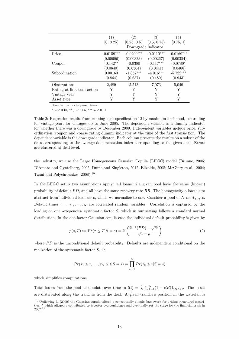
Table 2: Regression results from running logit specification 12 by maximum likelihood, controllingfor vintage year, for vintages up to June 2005. The dependent variable is a dummy indicatorfor whether there was a downgrade by December 2009. Independent variables include price, sub-ordination, coupon and coarse rating dummy indicator at the time of the first transaction. Thedependent variable is the downgrade indicator. Each column presents the results on a subset of thedata corresponding to the average documentation index corresponding to the given deal. Errorsare clustered at deal level.
the industry, we use the Large Homogeneous Gaussian Copula (LHGC) model (Brunne, 2006;
D’Amato and Gyntelberg, 2005; Duffie and Singleton, 2012; Elizalde, 2005; McGinty et al., 2004;
Tzani and Polychronakos, 2008).10
In the LHGC setup two assumptions apply: all loans in a given pool have the same (known)
probability of default PD, and all have the same recovery rate RR. The homogeneity allows us to
abstract from individual loan sizes, which we normalize to one. Consider a pool of N mortgages.
Default times τ = τ1, . . . , τN are correlated random variables. Correlation is captured by the
loading on one -exogenous- systematic factor S, which in our setting follows a standard normal
distribution. In the one-factor Gaussian copula case the individual default probability is given by
p(s, T ) := Pr(τ ≤ T |S = s) = Φ
(Φ−1(PD)−√ρs
√1− ρ
)(2)
where PD is the unconditional default probability. Defaults are independent conditional on the
realization of the systematic factor S, i.e.
Pr(τ1 ≤ t, . . . , τN ≤ t|S = s) =
N∏k=1
Pr(τk ≤ t|S = s)
which simplifies computations.
Total losses from the pool accumulate over time to l(t) = 1N
∑Nk=1(1 − RR)1(τk≤t). The losses
are distributed along the tranches from the deal. A given tranche’s position in the waterfall is
10Following Li (2000) the Gaussian copula offered a conceptually simple framework for pricing structured securi-ties,11 which allegedly contributed to investor overconfidence and eventually set the stage for the financial crisis in2007.12
13

(1) (2) (3) (4)
[0, 0.25) [0.25, 0.5) [0.5, 0.75) [0.75, 1]Downgrade indicator - AAA only
Price -0.0352∗∗∗ -0.0360∗∗∗ -0.0347∗∗∗ -0.0539∗∗∗
(0.00900) (0.00529) (0.00632) (0.0127)Coupon 0.0508∗∗∗ 0.0546 0.0919 0.118∗
(0.0161) (0.0451) (0.0575) (0.0625)Subordination -0.0174 -2.774∗∗ -2.014 -9.907∗∗∗
(1.622) (1.229) (1.881) (3.612)Observations 1,325 3,073 3,272 2,926Rating at first transaction Y Y Y YVintage year Y Y Y YAsset type Y Y Y Y
Downgrade indicator - not AAA
Price -0.0163∗∗ -0.0129∗∗∗ -0.00786∗∗∗ -0.0113∗∗∗
(0.00714) (0.00371) (0.00250) (0.00358)Coupon -0.367∗∗∗ -0.167∗∗∗ -0.201∗∗∗ -0.156∗∗∗
(0.102) (0.0475) (0.0529) (0.0603)Subordination -0.309 -2.648∗∗∗ -4.501∗∗∗ -4.193∗∗∗
(1.881) (0.880) (0.538) (0.784)Observations 1,038 2,248 3,757 2,111Rating at first transaction Y Y Y YVintage year Y Y Y YAsset type Y Y Y Y
Standard errors in parentheses∗ p < 0.10, ∗∗ p < 0.05, ∗∗∗ p < 0.01
Table 3: Regression results from running logit specification 12 by maximum likelihood, controllingfor vintage year, for vintages up to June 2005. The dependent variable is a dummy indicatorfor whether there was a downgrade by December 2009. Independent variables include price, sub-ordination, coupon and coarse rating dummy indicator at the time of the first transaction. Thedependent variable is the downgrade indicator. Each column presents the results on a subset of thedata corresponding to the average documentation index corresponding to the given deal. Errorsare clustered at deal level.
14

characterized by its lower and upper attachment points a and b where 0 ≤ a < b ≤ 1. Its notional
is a proportion b− a of the total pool notional N . The losses borne by this tranche are given by
l[a,b](t) =[l(t)− a]+ − [l(t)− b]−
b− a.
This exposure to risk affects the expected payoff of the CMO tranche. Using the recovery rate,
equation (2) yields the following estimate of expected losses within the [a, b] tranche by payment
date Ti:
E[l[a,b](Ti)] =1
b− a
∫ ∞−∞
e−s2/2
√2π
([(1−RR)p(s, Ti)− a]+ − [(1−RR)p(s, Ti)− b]+
)ds (3)
Duffie and Garleanu (2001) and Coval et al. (2009a) look at the sensitivity of expected recovery to
default correlation. Figure 3.1 replicates the exercise in Coval et al. (2009a) by plotting expected
recovery for each value of ρ, normalized by the value corresponding to ρ = 20%.
Figure 3.1: Sensitivity of a simulated CMO structure to default correlations. We plot the expectedpayoff within a given tranche, for each value of the underlying correlation ρ (parameters are PD=5%and LGD=50% as in Coval et al. (2009a)). The results are normalized by baseline estimate,based on the same parameters and a correlation ρ = 20%. No prepayments are incorporated (i.e.SMM=0%) for comparability of outcomes.
Using payment dates 0 < T1 < · · · < Tm = T (where T is the maturity of the security), write the
pricing equation of the security
V[a,b]
N(b− a)=c
m∑i=1
B(0, Ti)∆(Ti−1, Ti)(1− l[a,b](Ti)). (4)
Formula (4) equates current price to the sum (in expectation) of two terms: the discounted cash-
flows from coupon payments and the residual value (after accounting for defaults) of principal out-
standing. Here B(t1, t2) discounts a payoff at t2 to t1, c denotes the tranche coupon and ∆(Ti−1, Ti)
is the time difference between two payment dates (for mortgage bonds we use ∆(Ti−1, Ti) ≡ 1/12).
15

The pricing equation is then pN(b − a) = E[V[a,b]]. Writing e[a,b]i = E[1 − l[a,b](Ti)] the following
holds at origination:13
p0 =c
m∑i=1
B(0, Ti)∆(Ti−1, Ti)e[a,b]i (5)
The pool is exposed to prepayment risk.14 As prepayments happen, the coupon rate is applied
to the balance outstanding, while the prepaid amount is allocated across tranches according to
the order specified in the prospectus. In the absence of data about the order of the cashflows for
each deal, we make the simplifying assumption that prepayments are uniformly distributed across
tranches.15 We obtain
pt =
m∑i=t+1
B(t, Ti)e[a,b]i
i−1∏k=t+1
(1− SMMk)
c∆(Ti−1, Ti)(1− SMMi)︸ ︷︷ ︸coupon payment
+ SMMi︸ ︷︷ ︸prepaid principal
(6)
where SMMk is the single month mortality rate at time k, and is given by the PSA. Given the
unconditional default probability PD, the recovery rate RR and prepayment rate SMMk, pricing
equation (6) pins down a value of ρ, the market estimate of default correlation for the given pool
of loans. Note that expression (2) is only defined for ρ ∈ [0, 1) and thus the existence of a solution
to equation (6) is not guaranteed for an arbitrary choice of p and c. So instead of solving the
equation, we solve
minρ∈[0,1)
∣∣∣∣∣pt −m∑
i=t+1
B(t, Ti)e[a,b]i
i−1∏k=t+1
(1− SMMk) (c∆(Ti−1, Ti)(1− SMMi) + SMMi)
∣∣∣∣∣ (7)
Note that expected losses are monotonically increasing in default correlation ρ for the senior
tranche, and monotonically decreasing for the junior tranche (see Figure 3.1). The mezzanine
tranche behaves like a senior tranche for low correlations and like a junior tranche for high ones
(Ashcraft and Schuermann, 2008; Duffie, 2008).16 This gives the market estimate of default corre-
lations which we now compute on our panel of security prices.
13Note that formula (6) implies that default occurs immediately after the following period payment.14The Standard Prepayment Model of The Bond Market Association specifies a prepayment percentage for each
month in the life of the underlying mortgages, expressed on an annualized basis. In Section H we will use thecommon assumption that prepayment speed is given by 150% PSA (see Figure C.10).
15As an example, Duffie and Singleton (2012) discuss two prioritization schemes (uniform and fast). Both implyprepayment cash flows are sequential over seniorities. We do not have deal-level information about the allocationof cash flows, and so we prepayments in a way that is neutral across deals.
16For those cases two minima could arise in principle (as would also be the case if solving for equation (6) insteadof (7)).
16

3.1 Model parameters: default and prepayment
3.1.1 Probability of default and recovery rate
Our analysis is focused on expected losses (EL). Equation 3 uses the identity EL = PD × LGD,
which requires both default and recovery to be based on the same event. Recoveries in our data
are based on liquidated values, hence the use of liquidation as the default event.
Figure C.7 shows an increase in liquidation rates in the running to the crisis, though the trend
is only upward sloping from 2005 vintages onward. Using securitization data from ABSNet and
default experience from CoreLogics, Ashcraft et al. (2011) study MBS ratings and default rates
in the running to the crisis. We look at the cumulative rate of liquidation, whereas they consider
90+ delinquency rates over 12 months. Alt-A default rates were roughly half those of subprime
deals until early 2005, when both rates soared in the running to the crisis. By 2008, securitization
issuance had dropped to the extent that errors bands in our sample overlap. One difference is
that while the 90+ delinquency rate they report remains lower for Alt-A deals, we find that their
cumulative liquidation rate, initially similar to that of prime deals, caught up with that of subprime
in the running to the crisis.
From loss event data we can compute LGDs at deal level (see Figure C.14 for a count of observations
by vintage and asset type). Figure C.8 shows that LGD was nearly monotonically increasing from
1990 onwards (except for a peak in 1996) in the running to 2007, so that the possibility that
investors were adjusting their expectations of LGD over the cycle must be taken into account.
However, for LGDs to be computed the full post-workout must be observed, which usually takes
a substantial observation time after default. Recent advances in modeling LGDs with incomplete
workouts (see Rapisarda and Echeverry (2013)) have been far from the norm in the industry,
especially in the running to the crisis. We will apply the common assumption of constant LGD,
using the long run (weighted) average on our sample of 59.87%, virtually the same as the 60%
typically assumed in the literature (Altman, 2006; Brunne, 2006; Coval, Jurek, and Stafford, 2009b;
Hull and White, 2004, 2008).
Investors’ beliefs about default rates are elicited with a regression model establishing the like-
lihood of default as a function of loan covariates and estimated on default history. Similarly
we use a proportional hazard model on a prepayment indicator to assess investors’ beliefs about
prepayment speeds. The model is estimated as a separable hazard model, treating observations
representing default as censored as in Palmer (2015) and Liu (2016). Default and prepayment are
termination reasons happening at a random time τ term, whose intensity (for termination cause
term ∈ {default, prepayment}) is given by equation (8).
λtermi (t) = limε→0
Pri(t− ε < τ term ≤ t | t− ε < τ term, X)
ε. (8)
17

Here i denotes loan, and t denotes time after origination. The density function in equation 8 is
modeled as
λtermi (t)
λterm0 (t)= exp(X ′itβ
term) (9)
whereλterm0 (t)is the baseline hazard function that depends only on the time since origination t.
Covariates in Xit include loan attributes (loan amount, coupon gap relative to 10 year constant
maturity Treasury, LTV, prepayment penalty indicator), agent characteristics (FICO score, owner
occupancy) and variables at the CBSA level such as home price appreciation and unemployment
rate. The exponential model specified in equation 8 has a continuous time specification. To
estimate it on discrete time data we accumulate the intensity process λ over time intervals per
equation (10).
Pri(t < τ term | t− 1 < τ term) = exp
(−∫ t
t−1λtermi (u)du
)(10)
This leads to the complementary log-log specification in equation (11):
Pri(t < τ term | t− 1 < τ term) = exp(− exp(X ′itβterm)λterm0 (t)) (11)
We estimate specification (11) on data up to the end of 2004, with month since origination fixed
effects to obtain the hazard functions over the first 60 months of the loan. We document the
results in Table 35 and plot the resulting prepayment rates on Figure 3.2. We find that adjustable
rate mortgages are both more likely to default and prepay than fixed rate types. Subprime loans
are the asset type most likely to default. In terms of prepayment hazard, there is no significant
difference across asset types other than prime loans being less subject to prepayment than other
types.
We now compare our results with the ones obtained by Liu (2016) who uses the same model
to estimate default and prepayment hazard rates on loans backed by the government-sponsored
entities (Fannie Mae and Freddie Mac).17 On one hand, we find the same sign for the effect of
FICO score, the difference between the original loan interest rate and the original 10 year rate and
17Adding late originations (up to 2007) we find a number of similarities. The main difference that arises is thatnow subprime loans can be seen to be prepaying significantly more than other types, and significantly more thanearly vintages. This suggests that the link between subprime origination and home prices through prepaymentswas specific to the pre-crisis boom rather than a constitutive characteristic of subprime loans from their inception.Macroeconomic factors such as home price appreciation and unemployment exhibit a similar effect on defaults andprepayments when adding late vintages. Instead, for coupon gap there is a change compared to the early sample.The coupon gap, i.e. the change in 10 year rates between origination and present, reflects stronger incentives torefinance. The expectation is that this leads to a higher probability of prepayment and a lower probability of default,which we see once we add late cohorts but not in the early sample.
18

(a) Prepayment hazard (b) Cumulative prepayment rate
Figure 3.2: Marginal and cumulative prepayment rates implied from the model (11), as summarizedin Table 36. Using loan covariates at origination, prepayment hazard rates are computed at theloan level. Averages are computed by asset type and month after origination, and plotted here.
the unemployment rate. Moreover, in terms of default hazard we find similar effects of LTV and
home price appreciation.
On the other hand we find a few differences, mostly about the link between home prices and
prepayment rates. Liu (2016) finds that home price appreciation increases prepayment hazard
while we find the opposite. Similarly, he finds that higher LTV reduces prepayment hazard while
we find no clear link. As discussed by Gorton (2009), while the prepayment option is always
valuable for prime, 30-year fixed rate mortgages (i.e. if house prices rise borrowers build up
equity), for subprime loans lenders hold an implicit option to benefit from house price changes.
Table 35 shows prepayment penalties, this being the way in which the lender exercises its option,
are a strong deterrent against this termination type.
The break-even probabilities of a crisis computed by Beltran, Cordell, and Thomas (2017) from
CDO prices show a decrease from early cohorts (pre 2006 per their definition) to late ones, which
suggests a relatively high risk premium was charged in early cohorts. Though there are no studies
on risk premia in mortgage markets, we can benchmark our parameters against the corporate
market. (Berndt, Douglas, Duffie, Ferguson, and Schranz, 2005) imply actual and risk-neutral
probabilities from CDS market quotes. They find that the corresponding coverage factors (ratio of
risk neutral probability to real probability) oscillate between 1.5 and 3.5 over time, between 2002
and 2003. We use a coverage ratio of 3.18
Using the model in Table 36 we predict prepayment hazards and default probabilities at the loan
level, and average them at the deal level. Both the default probability and the hazard rate are
estimated deal by deal (in Section H we use a constant PD and prepayment speed, as a robustness
check). As for the prepayment hazard, we will use the full schedule in order to estimate the average
prepayment speed for the given deal over the first 60 months. As Figure 3.2 illustrates, subprime
18Heynderickx, Cariboni, Schoutens, and Smits (2016) quantify coverage factors from CDS quotes of Europeancorporates and find that they range between 1.27 for Caa (Moody’s) ratings to 13.51 for Aaa ones on pre-crisis data.Like Heynderickx et al. (2016), Denzler, Dacorogna, Muller, and McNeil (2006) argue that risk spreads exhibit ascaling law, whereby risk premia are decreasing in the probability of default. The results in Table 43 imply coverageratios between 2.03 for subprime deals and 3.27 for Alt-A ones, in line with the literature.
19

(a) Probability of default
Figure 3.3: Probability of default implied from the complementary log-log model, estimates ofwhich are in Table 36. Using loan covariates at origination, default probabilities are computed atthe loan level. Averages are computed by asset type and month after origination, and plotted here.
loans have the highest prepayment rates, followed by Alt-A loans. They also have the highest
default probabilities, as shown in Figure 3.3. We use the model-implied PDs from Table 36 (see
Figure 3.3) and include them as controls in our regressions.
Prepayments are contractually allocated across classes per the deal prospectus. Although we don’t
have information at deal-tranche level, a proxy we can look into is the rating at first transaction.
We split prepayment rates by tranche rating, assuming that prepayment behavior is driven by this
attribute. Although we do see mezzanine tranches dropping faster than senior ones, the ordering is
not monotonically increasing as BBB tranches are prepaying faster than AA ones (see Figure C.11).
For that reason we do not assume prepayments are sequential from AAA to D tranches.
Another model input is the residual maturity of the contract at the time of pricing. We source
contractual maturity from Bloomberg, which for most bonds is close to 30 years. These figures
are high (16.27 years difference on average, on a sample of 5,507 tranches) compared with realized
maturity (defined as the first observation where the tranche balance is zero). Figure C.9 also
suggests that bonds do not live that long on average. Adelino (2009) uses weighted average life
(WAL) instead of contract maturity, which is closer to the realized maturity. We also source WAL
for a sample of our loans where we could find it, but found that WALs are low compared to
realized maturities in the data (the average difference is 6.77 years on a sample of 16,894 tranches,
see Figure C.12 for a further breakdown of the difference). We will use contractual maturity,
relying on the assumption of 150% PSA to achieve an accurate reduction of tranche balance over
time.
The model in Table 36 incorporates all observations over time, applying them both prospectively
and retrospectively to price bonds over time. In reality, agents’ expectations about default evolve
20

over time, especially as the business cycle unfolds. As an example take home prices, which fluctuate
over the cycle. As Table 13 shows, home price appreciation is the variable whose effect on defaults
changes the most over the cycle. In particular, the negative relationship between price appreciation
and defaults documented in Table 36 is an average between the positive effect recorded in the early
years of the sample (up to 2002) and the negative effect in subsequent years. We expect that the
effect this has on the pricing model is small, given that over the times of the prices we are interested
in (mostly 2004 and 2005) the coefficients in Table 13 tend to be close to those in Table 36.
Loan performance data gives a basis for consensus about probability of default, loss given default
and prepayment speed. Default correlation is instead a parameter market participants are more
likely to disagree about19. Seeing these disagreements as the starting point for differential infor-
mation, we will use the pricing model from Section 3 to generate a summary statistic that acts as a
signal of future downgrades, and study how asset opacity drives the informativeness of the signal.
4 Implied default correlations from CMO data
For a given bond we compute its compound correlation ρ given the coupon rate c, market price
p, attachment and detachment points a ≥ 0 and a < b ≤ 1. The probability of default and
prepayment speed are estimated per Section 3.1. The recovery rate is RR = 60%. We use the
discount rate r = 4.27%, the average 10-year constant maturity treasury (annual) rate between 1995
and 2015. The numerical computations of loss probability are evaluated using a trapezoidal rule,
which Brunne (2006) deems faster than Gauss-Legendre and Gauss-Hermite methods. Figure C.16
provides a summary of observations.
The distribution of individual outcomes is bimodal (see Figure C.15). The extreme prices suggest
there is a role for market incompleteness as in Andreoli, Ballestra, and Pacelli (2016) and Stanton
and Wallace (2011). Tzani and Polychronakos (2008) find that in CDS markets model correlations
would often have had to exceed 100% in order to price supersenior tranches, which is suggested by
Figure H.1. Figure C.16 also shows evidence of a correlation smile in prices both before and after
the crisis.20
Using a one factor Gaussian copula model, Buzkova and Teply (2012) analyze prices of the 5-year,
North American investment grade CDX (V3) index between September 2007 and February 2009.
They report that for synthetic CDOs, implied correlations show a large increase, from 0.15 to 0.55
19“Currently, the weakest link in the risk measurement and pricing of CDOs is the modeling of default correlation.”citeDuffie:08
20The correlation smile is an artifact from the compound correlation method (O’Kane and Livesey, 2004). Amethod that is used to derive increasing correlations is the base correlation, which is computed as follows: let theattachment points in the full waterfall be given by (b1, . . . , bn), where bn = 1. First, solve 6 for the tranche [0, bk],
k = 1 . . . n. This gives an estimate of e[0,bk]i . Using the identity
(b− a)e[a,b]i = be
[0,b]i − ae
[0,a]i ,
the expected losses in tranche [a, b] can be sequentially computed along the waterfall: once the [bk−1, bk] tranchehas been priced, the following one can be priced using
(bk+1 − bk)e[bk,bk+1]
i = bk+1e[0,bk+1]
i − bke[0,bk]i .
Base correlations price all tranches in a deal simultaneously, and thus do not use base correlations because we arepricing tranches that trade separately over time.
21

Figure 4.1: Average correlation plotted against tranche subordination percentage, on two givendates. We use the sample of early vintage bonds (originated prior to June 2005). Subordinations areassigned to 10 equally spaced bins. Within each subordination bin we plot the average correlation,along with vertical whiskers representing the standard error of the average.
on average over that time period. In comparison, we observe a significant increase over the same
period, though of smaller magnitude (from 0.89 to 0.93). Breaking the change by asset type we see
an increase for Alt-A tranches (from 0.81 to 0.97, significant at 99%) and for subprime deals (from
0.85 to 0.89, significant at 99%) and no change for prime ones (0.93). The upward adjustment was
thus the largest for Alt-A issues (see Figure C.17). In terms of seniorities, the difference observed
by Buzkova and Teply (2012) over the crisis is mainly driven by mezzanine tranches (7%-10% and
10%-15%). Figure C.16 also suggests the increase in correlations is larger among intermediate
seniorities.
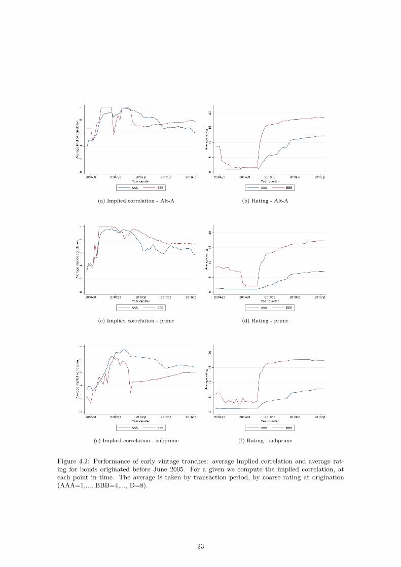
We now consider the trend over time (see Figure 4.2). Ratings were mostly stagnant ahead of the
crisis, especially for AAA tranches, in comparison with default correlations. BBB tranches even see
an improvement in ratings before the crisis while correlations are increasing (except for subprime
deals, which see both downwards and upwards changes). The sharpness of rating downgrades
suggests this is a concern for BBB tranches. Griffin and Tang (2012) argue that AAA ratings were
inflated in CDO securities, with optimistic ratings applied to a large share of bonds issued. Because
CDOs are mainly composed of CMO tranches, a potential channel for rating inflation in AAA CDO
tranches is rating inflation in the underlying BBB tranches, which were on average being upgraded.
This gives a possible channel for ratings inflation that differs boom time originations.
The graphic evidence presented so far suggests there is an adjustment of correlations over time,
and that ratings do not lead correlations at either maturity. Whether this means investors learn
faster than ratings agencies will be revealed by the informativeness of default correlations relative
to that of agency ratings. Using our panel data on prices and ratings, the next section will study
22
(a) Implied correlation - Alt-A (b) Rating - Alt-A
(c) Implied correlation - prime (d) Rating - prime
(e) Implied correlation - subprime (f) Rating - subprime
Figure 4.2: Performance of early vintage tranches: average implied correlation and average rat-ing for bonds originated before June 2005. For a given we compute the implied correlation, ateach point in time. The average is taken by transaction period, by coarse rating at origination(AAA=1,..., BBB=4,..., D=8).
23

the information content of market prices, as captured by implied correlations, about posterior bond
outcomes.
5 The information content of implied correlations
This section will focus on whether correlations implied from early prices are informative of sub-
sequent downgrades. We start with the sample of early vintages -prior to June 2005- for which
we have price data prior to the crisis. Using this data we replicate the findings by Ashcraft et al.
(2011) that market prices contain information about bond performance which is not captured by
the agency ratings. Then we replicate the result in Adelino (2009) that the information content
is a priori less significant for AAA tranches than for non-AAA tranches. The dependent variable
is whether bond i was downgraded by December 2009. We start with a logit specification similar
to that in Adelino (2009), where bond downgrade is the dependent variable. More specifically we
write
downgradei,2009 = f(α+ βρi0 + ηratingi0 + γXi0 + εi). (12)
The independent variable of interest is the implied correlation at first transaction ρi0. High cor-
relations are detrimental to senior bondholders but beneficial to subordinate ones (Duffie and
Garleanu, 2001). In line with this we expect that (except for bonds with zero subordination per-
centage, which we do not often observe) a higher implied correlation should predict a more likely
downgrade. We control for rating at origination using dummy indicators and for vintage year.
Also we cluster standard errors in all tests at the deal level, to control for the fact that several
classes in the same deal are often (down)graded at the same time.
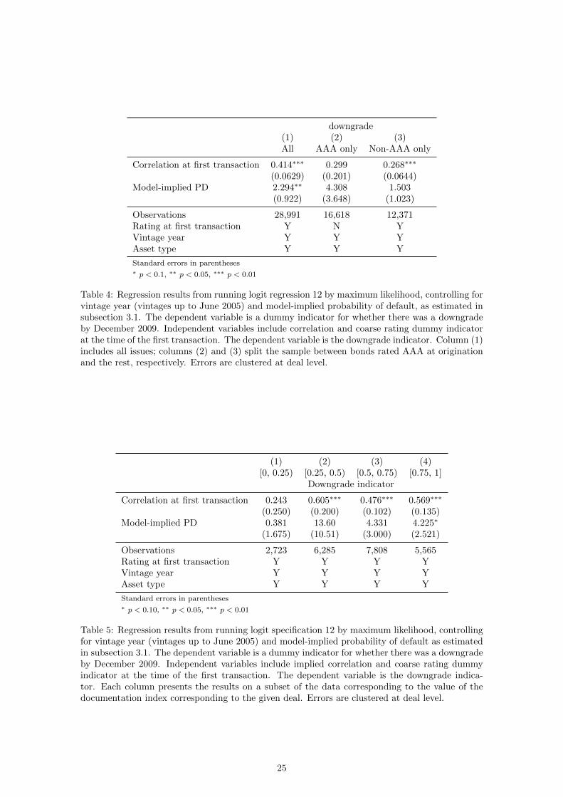
The results in Table 37 replicate the findings by Ashcraft et al. (2011) that, though statistically
significant, ratings at origination are not sufficient for implied correlations (in their case, coupon
premium) in predicting subsequent bond downgrades. Their proxy for the bond price is the coupon
premium to treasury, the hypothesis being that higher premium is reflective of more risk and thus
of more downgrades. Our implied correlation measure gives a similar result. We find a positive,
significant coefficient, so that higher implied correlation increases the likelihood of downgrades.
Table 37 breaks down this result between bonds initially rated AAA and the rest. While the
coefficient for correlation at first transaction remains significant for grades below AAA, implied
correlations seem to have no predictive power in terms of bond downgrades, similar to the findings
in Adelino (2009).
We use our opacity index to break down the sample by increments of 0.25, and present the results
in Table 38. We find a ranking along the index similar to the one discussed in Section 3, whereby
the coefficient on implied correlations is monotonically increasing in the value of the opacity index,
from insignificant at 10% for tranches below 0.25 to positive and significant at 1% for tranches
above 0.75.
24
downgrade(1) (2) (3)All AAA only Non-AAA only
Correlation at first transaction 0.414∗∗∗ 0.299 0.268∗∗∗
(0.0629) (0.201) (0.0644)Model-implied PD 2.294∗∗ 4.308 1.503
(0.922) (3.648) (1.023)
Observations 28,991 16,618 12,371Rating at first transaction Y N YVintage year Y Y YAsset type Y Y Y
Standard errors in parentheses∗ p < 0.1, ∗∗ p < 0.05, ∗∗∗ p < 0.01
Table 4: Regression results from running logit regression 12 by maximum likelihood, controlling forvintage year (vintages up to June 2005) and model-implied probability of default, as estimated insubsection 3.1. The dependent variable is a dummy indicator for whether there was a downgradeby December 2009. Independent variables include correlation and coarse rating dummy indicatorat the time of the first transaction. The dependent variable is the downgrade indicator. Column (1)includes all issues; columns (2) and (3) split the sample between bonds rated AAA at originationand the rest, respectively. Errors are clustered at deal level.
(1) (2) (3) (4)[0, 0.25) [0.25, 0.5) [0.5, 0.75) [0.75, 1]
Downgrade indicator
Correlation at first transaction 0.243 0.605∗∗∗ 0.476∗∗∗ 0.569∗∗∗
(0.250) (0.200) (0.102) (0.135)Model-implied PD 0.381 13.60 4.331 4.225∗
(1.675) (10.51) (3.000) (2.521)
Observations 2,723 6,285 7,808 5,565Rating at first transaction Y Y Y YVintage year Y Y Y YAsset type Y Y Y Y
Standard errors in parentheses∗ p < 0.10, ∗∗ p < 0.05, ∗∗∗ p < 0.01
Table 5: Regression results from running logit specification 12 by maximum likelihood, controllingfor vintage year (vintages up to June 2005) and model-implied probability of default as estimatedin subsection 3.1. The dependent variable is a dummy indicator for whether there was a downgradeby December 2009. Independent variables include implied correlation and coarse rating dummyindicator at the time of the first transaction. The dependent variable is the downgrade indica-tor. Each column presents the results on a subset of the data corresponding to the value of thedocumentation index corresponding to the given deal. Errors are clustered at deal level.
25
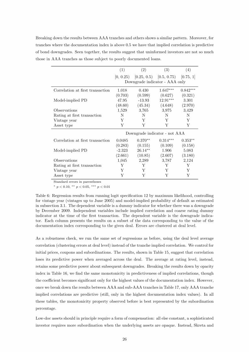
Breaking down the results between AAA tranches and others shows a similar pattern. Moreover, for
tranches where the documentation index is above 0.5 we have that implied correlation is predictive
of bond downgrades. Seen together, the results suggest that uninformed investors are not so much
those in AAA tranches as those subject to poorly documented loans.
(1) (2) (3) (4)
[0, 0.25) [0.25, 0.5) [0.5, 0.75) [0.75, 1]Downgrade indicator - AAA only
Correlation at first transaction 1.018 0.430 1.647∗∗∗ 0.842∗∗∗
(0.703) (0.599) (0.627) (0.321)Model-implied PD 47.95 -13.93 12.91∗∗∗ 3.301
(48.60) (45.34) (4.648) (2.970)Observations 1,529 3,765 3,975 3,429Rating at first transaction N N N NVintage year Y Y Y YAsset type Y Y Y Y
Downgrade indicator - not AAA
Correlation at first transaction 0.0485 0.370∗∗ 0.314∗∗∗ 0.353∗∗
(0.283) (0.155) (0.109) (0.158)Model-implied PD -2.323 26.14∗∗ 1.906 5.083
(2.661) (10.85) (2.607) (3.180)Observations 1,045 2,289 3,787 2,124Rating at first transaction Y Y Y YVintage year Y Y Y YAsset type Y Y Y Y
Standard errors in parentheses∗ p < 0.10, ∗∗ p < 0.05, ∗∗∗ p < 0.01
Table 6: Regression results from running logit specification 12 by maximum likelihood, controllingfor vintage year (vintages up to June 2005) and model-implied probability of default as estimatedin subsection 3.1. The dependent variable is a dummy indicator for whether there was a downgradeby December 2009. Independent variables include implied correlation and coarse rating dummyindicator at the time of the first transaction. The dependent variable is the downgrade indica-tor. Each column presents the results on a subset of the data corresponding to the value of thedocumentation index corresponding to the given deal. Errors are clustered at deal level.
As a robustness check, we run the same set of regressions as before, using the deal level average
correlation (clustering errors at deal level) instead of the tranche implied correlation. We control for
initial prices, coupons and subordinations. The results, shown in Table 15, suggest that correlation
loses its predictive power when averaged across the deal. The average at rating level, instead,
retains some predictive power about subsequent downgrades. Breaking the results down by opacity
index in Table 16, we find the same monotonicity in predictiveness of implied correlations, though
the coefficient becomes significant only for the highest values of the documentation index. However,
once we break down the results between AAA and sub-AAA tranches in Table 17, only AAA tranche
implied correlations are predictive (still, only in the highest documentation index values). In all
these tables, the monotonicity property observed before is best represented by the subordination
percentage.
Low-doc assets should in principle require a form of compensation: all else constant, a sophisticated
investor requires more subordination when the underlying assets are opaque. Instead, Skreta and
26

Veldkamp (2009) predict that rating inflation is worse when assessing the true value of the asset is
difficult (making ratings noisier and more varied). For their result to hold, investors must be unable
to infer the rating selection bias. Similarly in our case, investors who are unaware of the deficiency
in documentation are more likely to be subjected to inflated ratings. Table 40 provides evidence
that AAA share at origination is decreasing in our opacity index (controlling for the model-implied
probability of default). This suggests that unsophisticated investors select into low-doc deals,
where rating inflation is more likely to occur.
6 Conclusion
Two key frictions take place in securitization markets between the investor and the securitizer.
Though there is a role for a proxy of investor unsophistication, namely whether the bond is AAA-
rated at origination, there is an important role of asset opacity, which we capture using a deal-level
index of documentation completeness. We observe less of a differential in information content
across seniorities than across low-doc assets and “full-doc” ones. We show that the latter exhibit
better information content across the rating spectrum. In particular, AAA implied correlations
are no less predictive than the rest when the bond comes from a deal with a high standard of
documentation.
We link the information content of bond trades to the opacity on the underlying collateral, saying
that more opaque loans convey less market information. The results suggest that unsophisticated
transactions select into low-doc deals. In line with this, we provide evidence that more opaque
deals tend to issue a higher proportion of AAA bonds, controlling for risk attributes of the deal.
The results are consistent with ratings inflation.
Implied correlations are large in subprime deals compared to other asset classes, which reflects a
design feature of subprime loans that made them jointly dependent on house prices. We capture
this within a systematic factor framework. However, investors could be underestimating aspects of
default clustering different from systematic risk. Following Griffin and Nickerson (2016), who argue
rating agencies underestimate frailty risk, the question of whether contagion risk (see Appendix J)
is priced remains open.
27
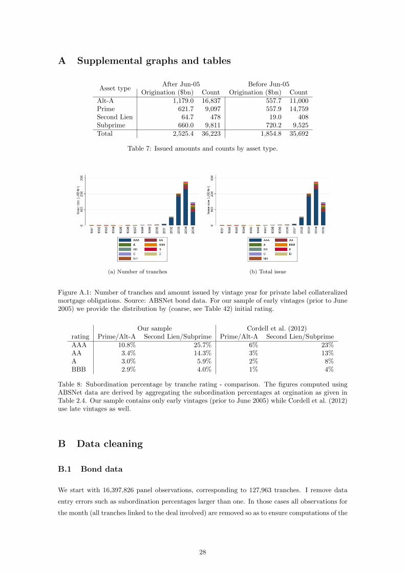
A Supplemental graphs and tables
Asset typeAfter Jun-05 Before Jun-05
Origination ($bn) Count Origination ($bn) CountAlt-A 1,179.0 16,837 557.7 11,000Prime 621.7 9,097 557.9 14,759Second Lien 64.7 478 19.0 408Subprime 660.0 9,811 720.2 9,525Total 2,525.4 36,223 1,854.8 35,692
Table 7: Issued amounts and counts by asset type.
(a) Number of tranches (b) Total issue
Figure A.1: Number of tranches and amount issued by vintage year for private label collateralizedmortgage obligations. Source: ABSNet bond data. For our sample of early vintages (prior to June2005) we provide the distribution by (coarse, see Table 42) initial rating.
Our sample Cordell et al. (2012)rating Prime/Alt-A Second Lien/Subprime Prime/Alt-A Second Lien/SubprimeAAA 10.8% 25.7% 6% 23%AA 3.4% 14.3% 3% 13%A 3.0% 5.9% 2% 8%BBB 2.9% 4.0% 1% 4%
Table 8: Subordination percentage by tranche rating - comparison. The figures computed usingABSNet data are derived by aggregating the subordination percentages at orgination as given inTable 2.4. Our sample contains only early vintages (prior to June 2005) while Cordell et al. (2012)use late vintages as well.
B Data cleaning
B.1 Bond data
We start with 16,397,826 panel observations, corresponding to 127,963 tranches. I remove data
entry errors such as subordination percentages larger than one. In those cases all observations for
the month (all tranches linked to the deal involved) are removed so as to ensure computations of the
28

YearABSNet sample Adelino (2009)
Origination ($bn) Count Origination ($bn) Count≤2002 319.3 5,438
2003 470.5 10,120 496.5 8,5742004 677.4 12,519 767.3 11,4602005 904.5 16,684 1,058.5 17,1352006 1,038.0 15,022 1,080.4 18,2062007 939.4 11,716 802.1 12,037≥2008 31.2 177Total 4,380.3 71,676 4,204.8 67,412
Table 9: Origination amounts and counts at origination, by vintage year, compared to the samplein Adelino (2009).
Figure A.2: Average tranche price by age of the bond in months. For our sample of bonds originatedin 2004 and 2005 we compute the average price by the time elapsed (in months) since the bondissue. Vertical whiskers show the standard errors.
(1) (2)
Asset type Early vintages Late vintages
Alt-A 7.5% 19.5%
Prime 2.3% 6.6%
Second Lien 7.2% 25.8%
Subprime 14.8% 30.5%
Observations 4,060,698 631,793
Table 10: Liquidation rates from the loan sample. Column (1) calculates the percentage of loanslinked to early vintage deals (before June 2005) that are liquidated. Column (2) calculates thesame ratio for late vintage loans.
29

Figure A.3: Average subordination difference between AAA and BBB bonds. Source: ABSNetbond data.The figure presents the difference between the average AAA and average BBB subor-dination over trading time (for early vintages, prior to June 2005) using the rating at the giventrading time. The difference is computed by asset type.
Figure A.4: Probability of default by vintage year. We compute the default rate for each of thedeals that compose our population, and then average by vintage year and asset type. The resultsare presented here along with standard error bands around the average.
30

Figure A.5: Percentage loss given default by vintage year. The aggregate loss given default iscomputed from the sample of loans associated to the deals that compose our population of CMOs.
Figure A.6: Average class balance factor by asset class over tranche age. Alongside the averages,we compute the balance factor that results from a 150% payment schedule alone (excluding plannedamortization).
31

Figure A.7: Standard Prepayment Model of The Bond Market Association. Prepayment percentagefor each month in the life of the underlying mortgages, expressed on an annualized basis.
Figure A.8: Plot of average class factor against tranche age by tranche initial rating.
32

(a) Average realized
(b) WAL
Figure A.9: Average realized and weighted average life by coarse rating and asset type. The secondpanel includes observations where we found a matching WAL in Bloomberg.
33

Figure A.10: Proportion of ARM loans by vintage and asset type.
Figure A.11: Number of deals originated by asset type and vintage year.
34
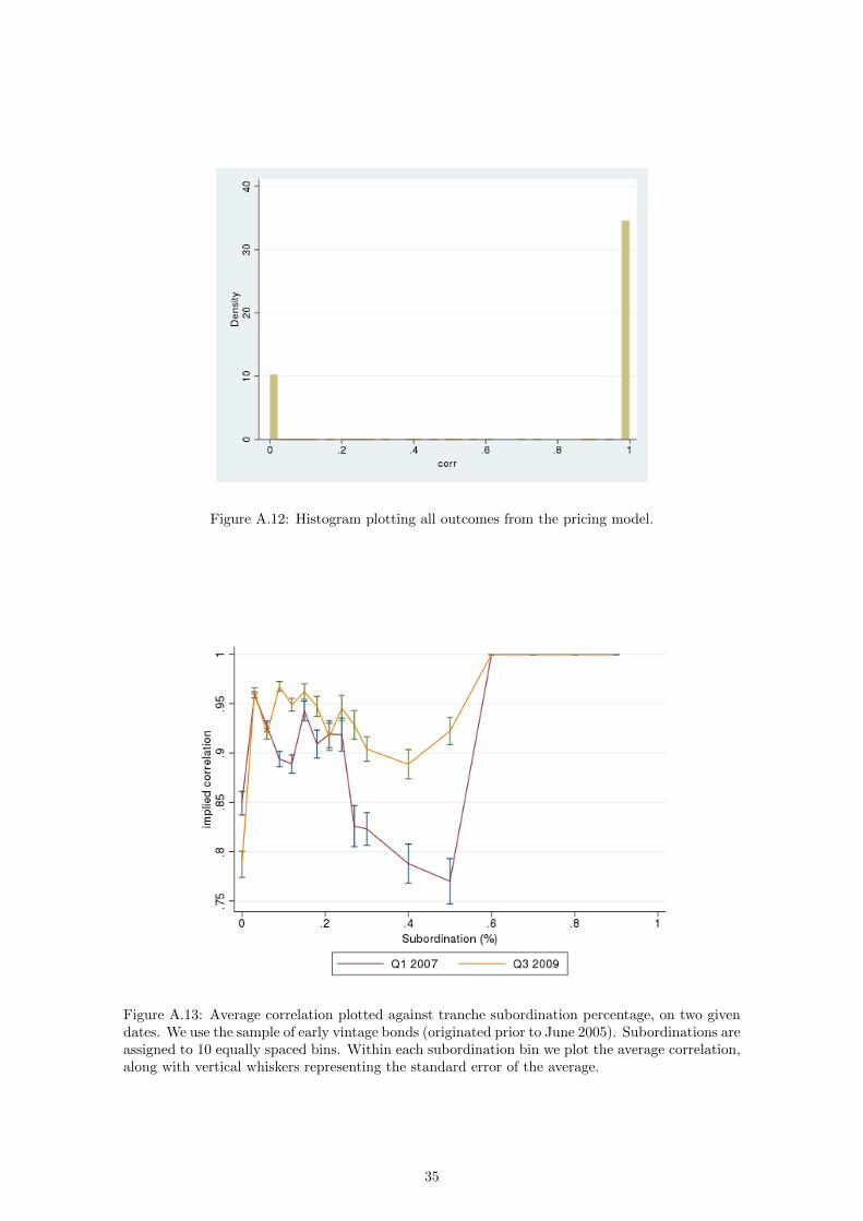
Figure A.12: Histogram plotting all outcomes from the pricing model.
Figure A.13: Average correlation plotted against tranche subordination percentage, on two givendates. We use the sample of early vintage bonds (originated prior to June 2005). Subordinations areassigned to 10 equally spaced bins. Within each subordination bin we plot the average correlation,along with vertical whiskers representing the standard error of the average.
35

(a) Alt-A
(b) Prime
(c) Subprime
Figure A.14: Average correlation plotted against tranche subordination percentage, on two givendates. Subordination values are assigned to 10 equally spaced bins. Within each subordinationbin we plot the average correlation, along with vertical whiskers representing the standard error ofthe average.
36

with data up to 2004 with data up to 2007(1) (2) (3) (4)Default Prepayment Default Prepayment
log(FICO) -1.468*** 1.408*** -2.076*** 0.305**-0.157 -0.155 -0.199 -0.12
owner occupied 0.039 -0.024 -0.098* 0.024-0.05 -0.02 -0.054 -0.02
original r - original 10 year rate 0.475*** 0.249*** 0.252*** 0.066***-0.01 -0.017 -0.011 -0.006
log(original amount) 0.421*** 0.257*** 0.143*** 0.02-0.043 -0.031 -0.041 -0.026
log(original LTV) 0.439*** -0.007 0.183*** 0.069***-0.043 -0.036 -0.033 -0.02
prepayment penalty -1.866*** -1.034*** -0.914*** -0.950***-0.08 -0.073 -0.031 -0.025
adjustable rate mortgage 0.655*** 0.493*** 0.367*** 0.467***-0.062 -0.047 -0.038 -0.015
log(Cumulative HPA) -8.398*** -7.780*** -6.482*** -2.474***-1.041 -0.963 -0.652 -0.41
coupon gap 0.400*** 0.120* -0.255*** -0.144**-0.05 -0.062 -0.04 -0.06
unemployment 0.330*** 0.320*** 0.201*** 0.319***-0.072 -0.075 -0.068 -0.075
Asset type: Prime -1.008*** -0.147*** -1.130*** -0.603***-0.078 -0.027 -0.078 -0.033
Asset type: Second Lien -0.580*** 0.124 0.843*** 0.385***-0.142 -0.079 -0.064 -0.028
Asset type: Subprime 0.504*** -0.021 1.113*** 0.201***-0.053 -0.05 -0.037 -0.02
CBSA FE Y Y Y YMonth since origination FE Y Y Y YObservations 68,634,789 76,206,672 121,236,208 126,625,633
Standard errors in parentheses∗ p < 0.1, ∗∗ p < 0.05, ∗∗∗ p < 0.01
Table 11: This table shows estimates using the maximum likelihood estimation of the complemen-tary log-log specification in (11), using a nonparametric baseline hazard, on the loan level dataavailable from ABSNet for private label loans (purchases only). The model treats competing risksindependently, indicating 1 for failure and 0 for censoring. Each coefficient is the effect of thecorresponding variable on the log hazard rate for either the default or prepayment of a mortgage.The conditional hazard is captured by performance month dummies, where performance is trackedover the first 60 months of the sample. The sample is truncated at December 2004 for columns (1)and (2), and at June 2007 for columns (3) and (4). Errors are clustered at CBSA level.
37
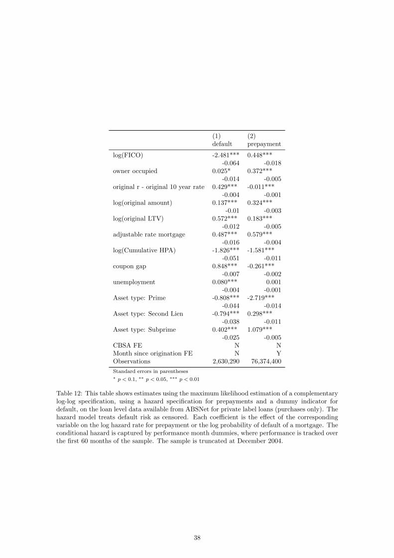
(1) (2)default prepayment
log(FICO) -2.481*** 0.448***-0.064 -0.018
owner occupied 0.025* 0.372***-0.014 -0.005
original r - original 10 year rate 0.429*** -0.011***-0.004 -0.001
log(original amount) 0.137*** 0.324***-0.01 -0.003
log(original LTV) 0.572*** 0.183***-0.012 -0.005
adjustable rate mortgage 0.487*** 0.579***-0.016 -0.004
log(Cumulative HPA) -1.826*** -1.581***-0.051 -0.011
coupon gap 0.848*** -0.261***-0.007 -0.002
unemployment 0.080*** 0.001-0.004 -0.001
Asset type: Prime -0.808*** -2.719***-0.044 -0.014
Asset type: Second Lien -0.794*** 0.298***-0.038 -0.011
Asset type: Subprime 0.402*** 1.079***-0.025 -0.005
CBSA FE N NMonth since origination FE N YObservations 2,630,290 76,374,400
Standard errors in parentheses∗ p < 0.1, ∗∗ p < 0.05, ∗∗∗ p < 0.01
Table 12: This table shows estimates using the maximum likelihood estimation of a complementarylog-log specification, using a hazard specification for prepayments and a dummy indicator fordefault, on the loan level data available from ABSNet for private label loans (purchases only). Thehazard model treats default risk as censored. Each coefficient is the effect of the correspondingvariable on the log hazard rate for prepayment or the log probability of default of a mortgage. Theconditional hazard is captured by performance month dummies, where performance is tracked overthe first 60 months of the sample. The sample is truncated at December 2004.
38
default
indicato
r(b
yth
eend
ofth
egiven
year)
2000
2001
2002
2003
2004
2005
2006
2007
2008
2009
log(F
ICO)
-2.485***
-3.599***
-4.816***
-2.583***
-3.141***
-3.682***
-4.561***
-4.160***
-3.029***
-2.059***
(0.494)
(0.257)
(0.151)
(0.101)
(0.071)
(0.052)
(0.038)
(0.027)
(0.018)
(0.014)
owneroccupied
-0.318**
0.037
0.263***
0.133***
-0.214***
-0.329***
-0.333***
-0.247***
-0.097***
-0.148***
(0.139)
(0.069)
(0.041)
(0.024)
(0.016)
(0.011)
(0.008)
(0.006)
(0.004)
(0.003)
originalr-original
-0.052
0.277***
0.199***
0.431***
0.459***
0.343***
0.164***
0.178***
0.158***
0.102***
10yearra
te(0
.038)
(0.018)
(0.011)
(0.006)
(0.004)
(0.003)
(0.002)
(0.001)
(0.001)
(0.001)
log(o
riginalamount)
-0.053
-0.038
-0.235***
0.125***
0.150***
-0.026***
-0.297***
-0.126***
-0.029***
-0.013***
(0.084)
(0.043)
(0.025)
(0.016)
(0.011)
(0.007)
(0.005)
(0.003)
(0.002)
(0.002)
log(o
riginalLTV)
0.828***
0.698***
0.585***
0.772***
0.682***
0.548***
0.445***
0.178***
0.124***
0.078***
(0.266)
(0.099)
(0.030)
(0.019)
(0.014)
(0.010)
(0.007)
(0.004)
(0.003)
(0.002)
adjustable
rate
-0.707***
0.145**
0.305***
0.335***
0.261***
0.269***
0.291***
-0.045***
-0.130***
0.001
mortgage
(0.104)
(0.058)
(0.035)
(0.023)
(0.016)
(0.011)
(0.008)
(0.006)
(0.004)
(0.003)
log(cumulativeHPA)
1.921***
2.981***
4.548***
-3.303***
-1.878***
-0.877***
0.412***
-1.998***
-5.796***
-4.319***
(0.676)
(0.248)
(0.122)
(0.103)
(0.054)
(0.030)
(0.018)
(0.017)
(0.011)
(0.007)
coupon
gap
-1.930***
0.216***
-0.591***
1.234***
0.998***
0.832***
0.170***
-1.057***
-0.810***
0.889***
(0.062)
(0.037)
(0.019)
(0.013)
(0.009)
(0.006)
(0.005)
(0.004)
(0.002)
(0.002)
unemployment
0.137***
-1.052***
-0.342***
-0.080***
0.011**
0.126***
0.176***
0.004***
-0.183***
-0.309***
(0.037)
(0.026)
(0.014)
(0.009)
(0.006)
(0.003)
(0.002)
(0.002)
(0.001)
(0.001)
Assetty
pe:Prime
0.000
-1.048***
-0.805***
-0.748***
-0.621***
-0.299***
-0.248***
-0.669***
-1.456***
-1.640***
(.)
(0.245)
(0.100)
(0.068)
(0.049)
(0.035)
(0.028)
(0.024)
(0.018)
(0.011)
Assetty
pe:Second
Lien
0.000
-3.509***
-5.936***
-4.410***
-1.984***
-0.213***
0.471***
0.877***
0.639***
0.616***
(.)
(1.012)
(1.002)
(0.271)
(0.062)
(0.027)
(0.018)
(0.012)
(0.007)
(0.005)
Assetty
pe:Subprime
2.872***
0.939***
0.213***
0.147***
0.274***
0.438***
0.742***
1.027***
0.777***
0.710***
(0.311)
(0.128)
(0.062)
(0.040)
(0.028)
(0.019)
(0.014)
(0.010)
(0.005)
(0.004)
Obs
230,631
516,866
865,545
1,435,035
2,630,290
4,307,739
5,766,680
6,014,866
6,014,866
6,014,866
Sta
nd
ard
erro
rsin
pare
nth
eses
∗p<
0.1
,∗∗
p<
0.0
5,∗∗
∗p<
0.0
1
Tab
le13
:T
his
tab
lesh
ows
esti
mat
esu
sin
gth
em
axim
um
like
lih
ood
esti
mati
on
of
aco
mp
lem
enta
rylo
g-l
og
spec
ifica
tion
,u
sin
ga
du
mm
yin
dic
ato
rfo
rd
efau
lt,
on
the
loan
leve
ld
ata
avai
lab
lefr
omA
BS
Net
for
pri
vate
lab
ello
an
s(p
urc
hase
son
ly).
For
each
year,
vari
ab
les
are
take
nat
the
mea
sure
men
tp
oin
t(e
ith
erd
efau
ltti
me,
ifd
efau
lted
,or
obse
rvat
ion
tim
e,w
hic
his
the
end
ofth
egiv
enye
ar)
.
39
(1) (2) (3) (4)AAA balance at origination as share of deal issuance
Opacity index -0.104∗∗∗ -0.0835∗∗∗ -0.101∗∗∗ -0.0259∗
(0.0154) (0.0153) (0.0151) (0.0151)
Observations 1,902 1,902 1,902 1,902Model-implied PD N Y Y YVintage year N N Y YAsset type N N N Y
Standard errors in parentheses∗ p < 0.10, ∗∗ p < 0.05, ∗∗∗ p < 0.01
Table 14: Regression results from running a linear regression at deal level of AAA origination (asshare of total) on the deal opacity index. Controls include model-implied PD, vintage year (weinclude vintages up to June 2005) and asset type.
downgrade(1) (2) (3)All AAA only Non-AAA only
Deal average correlation 0.211(0.189)
Average correlation within rating bucket 0.721∗ 0.369∗
(0.427) (0.217)Price -0.0185∗∗∗ -0.0446∗∗∗ -0.00937∗∗∗
(0.00152) (0.00305) (0.00150)Coupon -0.123∗∗∗ -0.0402 -0.183∗∗∗
(0.0178) (0.0245) (0.0240)Subordination -3.168∗∗∗ -4.144∗∗∗ -4.113∗∗∗
(0.271) (0.601) (0.316)
Observations 26,242 14,034 12,206Rating at first transaction Y N YVintage year Y Y YAsset type Y Y Y
Standard errors in parentheses∗ p < 0.1, ∗∗ p < 0.05, ∗∗∗ p < 0.01
Table 15: Regression results from running logit regression 12 by maximum likelihood, controllingfor vintage year (vintages up to June 2005) and model-implied probability of default, as estimatedin section 3.1. The dependent variable is a dummy indicator for whether there was a downgradeby December 2009. Column (1) includes all issues; columns (2) and (3) split the sample betweenbonds rated AAA at origination and the rest, respectively. Independent variables include deal levelaverage correlation (column 1), AAA average correlation (column 2), sub-AAA average correlation(column 3) and coarse rating dummy indicator at the time of the first transaction. The dependentvariable is the downgrade indicator. Errors are clustered at deal level.
40

(1) (2) (3) (4)[0, 0.25) [0.25, 0.5) [0.5, 0.75) [0.75, 1]
Downgrade indicator
Deal average correlation -0.581 -0.155 -0.0162 0.901∗∗
(0.750) (0.522) (0.367) (0.395)Price -0.0165∗∗∗ -0.0202∗∗∗ -0.0110∗∗∗ -0.0167∗∗∗
(0.00631) (0.00343) (0.00269) (0.00356)Coupon -0.134∗∗ -0.0369 -0.117∗∗∗ -0.0749
(0.0649) (0.0310) (0.0442) (0.0465)Subordination -0.0512 -1.869∗∗∗ -4.013∗∗∗ -5.858∗∗∗
(0.852) (0.653) (0.489) (0.959)
Observations 2,489 5,513 7,073 5,049Rating at first transaction Y Y Y YVintage year Y Y Y YAsset type Y Y Y Y
Standard errors in parentheses∗ p < 0.10, ∗∗ p < 0.05, ∗∗∗ p < 0.01
Table 16: Regression results from running logit specification 12 by maximum likelihood, controllingfor vintage year (vintages up to June 2005) and model-implied probability of default as estimatedin section 3.1. The dependent variable is a dummy indicator for whether there was a downgradeby December 2009. Independent variables include deal level average implied correlation and coarserating dummy indicator at the time of the first transaction. The dependent variable is the down-grade indicator. Each column presents the results on a subset of the data corresponding to thevalue of the documentation index corresponding to the given deal. Errors are clustered at deallevel.
tranching structure are correct.21 We follow Adelino (2009) in removing Interest Only, Principal
Only, Inverse Floater and Fixed to Variable bonds from the sample.
Notice that the most aggressive cleaning step is the removal of observations where price is missing.
As dicussed in section 2, this is due to the data gap that covers late (2005 and more recent)
vintages.
B.2 Loan level data
We start with a set of 22,008,610 loan originations. Of our originations set, 21,759,836 map to one
of our deal IDs. Below is a summary of deal level averages of certain covariates (FICO score, LTV,
private mortgage insurance coverage percentage) are computed.22
Historic data are contained in monthly reports. From the input 21,996,382 facilities we have at least
one observation for 17,350,072 of them. We recover a total 792,664,139 loan-month observations
from payment history (on average 45.7 obs per loan). From there we can compute default rates
at deal level. We have loss event data for 3,986,974 observations, linked to 5,965 deal IDs. From
there we can compute LGDs at deal level or vintage level.
21I manually computed subordination percentages on a random sample of deals to check the calculations byABSNet.
22Simple averages were preferred over weighted averages (weighted by e.g. the initial securitized balance) as thisreduces the number of missing observations.
41

(1) (2) (3) (4)
[0, 0.25) [0.25, 0.5) [0.5, 0.75) [0.75, 1]Downgrade indicator - AAA only
AAA average correlation 5.310 0.701 1.074 3.019∗∗∗
(3.508) (1.594) (0.962) (0.857)Price -0.0309∗∗∗ -0.0351∗∗∗ -0.0328∗∗∗ -0.0535∗∗∗
(0.00991) (0.00542) (0.00655) (0.0118)Coupon 0.0452∗∗∗ 0.0544 0.0898 0.149∗∗
(0.0173) (0.0453) (0.0580) (0.0726)Subordination 0.610 -2.791∗∗ -2.283 -11.79∗∗∗
(1.530) (1.260) (1.851) (4.377)Observations 1,325 3,073 3,272 2,926Rating at first transaction N N N NVintage year Y Y Y YAsset type Y Y Y Y
Downgrade indicator - not AAA
Below-AAA average correlation -1.266 0.527 -0.0727 0.195(0.886) (0.548) (0.431) (0.574)
Price -0.0154∗∗ -0.0127∗∗∗ -0.00783∗∗∗ -0.0115∗∗∗
(0.00704) (0.00370) (0.00249) (0.00362)Coupon -0.357∗∗∗ -0.174∗∗∗ -0.201∗∗∗ -0.155∗∗∗
(0.103) (0.0496) (0.0529) (0.0599)Subordination 0.133 -2.715∗∗∗ -4.482∗∗∗ -4.278∗∗∗
(1.905) (0.878) (0.541) (0.852)Observations 1,038 2,248 3,757 2,111Rating at first transaction Y Y Y YVintage year Y Y Y YAsset type Y Y Y Y
Standard errors in parentheses∗ p < 0.10, ∗∗ p < 0.05, ∗∗∗ p < 0.01
Table 17: Regression results from running logit specification 12 by maximum likelihood, controllingfor vintage year (vintages up to June 2005) and model-implied probability of default as estimatedin section 3.1. The dependent variable is a dummy indicator for whether there was a downgradeby December 2009. Independent variables include AAA average correlation (upper panel), sub-AAA average correlation (lower panel) and coarse rating dummy indicator at the time of the firsttransaction. The dependent variable is the downgrade indicator. Each column presents the resultson a subset of the data corresponding to the value of the documentation index corresponding tothe given deal. Errors are clustered at deal level.
(1) (2) (3) (4)AAA balance at origination as share of deal issuance
Opacity index -0.104∗∗∗ -0.0835∗∗∗ -0.101∗∗∗ -0.0259∗
(0.0154) (0.0153) (0.0151) (0.0151)
Observations 1,902 1,902 1,902 1,902Model-implied PD N Y Y YVintage year N N Y YAsset type N N N Y
Standard errors in parentheses∗ p < 0.10, ∗∗ p < 0.05, ∗∗∗ p < 0.01
Table 18: Regression results from running a linear regression at deal level of AAA origination (asshare of total) on the deal opacity index. Controls include model-implied PD, vintage year (weinclude vintages up to June 2005) and asset type.
42

Stage Tranches leftRemove deals that are entirely made of mixed asset types 119,215Remove deals where one tranche has subordination >1 119,215Remove observations with missing price 74,307Remove mixed-type asset pools 74,253Remove PO, IO, IF and FtV 71,950
Table 19: Data cleaning stages with number of tranches outstanding at the end of each step.
S&P rating Code Coarse rating CodeAAA 1 AAA 1AA+ 2 AA 2AA 3 AA 2AA- 4 AA 2A+ 5 A 3A 6 A 3A- 7 A 3BBB+ 8 BBB 4BBB 9 BBB 4BBB- 10 BBB 4BB+ 11 BB 5BB 12 BB 5BB- 13 BB 5B+ 14 B 6B 15 B 6B- 16 B 6CCC 17 C 7CCC- 18 C 7CC 19 C 7C 20 C 7D 21 D 8NR - NR -
Table 20: Mapping of ratings - fine and coarse level (with numbering code)
(a) FICO score (b) PMI coverage
Figure B.1: Distribution of covariates over time (vintage year).
43

(a) LTV (b) Original securitized balance
Figure B.2: Distribution of covariates over time (vintage year).
At the loan level, we keep only loans having purchase as purpose. This reduces the sample to
8,862,561 loans. Aside minor cleaning (originations before 1980, errors in time stamps) we arrive
to 7,145,251. From these we discard asset types other than Alt-A, Prime, Second Lien or Subprime
to arrive at the initial sample composed of early and late vintages.
C Variations on the baseline model
C.1 Pricing results with constant default probability and prepayment
speed
In this section we use a constant PD, by asset type, given as the
(1) (2) (3)
Asset type Early vintages Late vintages Model PD
Alt-A 7.5% 19.5% 24.5%
Prime 2.3% 6.6% 6.4%
Second Lien 7.2% 25.8% 21.1%
Subprime 14.8% 30.5% 30%
Observations 4,060,698 631,793 2,112
Table 21: Liquidation rates from the loan sample, and PD used for baseline estimation. Column(1) calculates the percentage of loans linked to early vintage deals (before June 2005) that areliquidated. Column (2) calculates the same ratio for late vintage loans. Column (3) shows the PDparameters used for the pricing model, calculated as the average of the deal level liquidation ratesfor both early and late deals.
After the collapse of private label securitization in 2007, most securitization conduits are insured
against default risk by the Government-Sponsored Entities (Fannie Mae and Freddie Mac), mak-
ing prepayment risk the most significant one in the literature. Schwartz and Torous (1989) and
Stanton (1995) measure the value of prepayment option in default-free securities (guaranteed by
the Government-Sponsored Entities). Downing, Stanton, and Wallace (2005) propose a two-factor
44

valuation model that distinguishes the separate, competing risks carried by the default and the
prepayment options. Sugimura (2004) develops an intensity model to price RMBS (pass-through)
bonds not insured against default risk, and thus exposed to both prepayment and default risk (but
credit events in his approach are assumed to be uncorrelated). We seek an accurate measure of
prepayment while keeping the focus on default risk, hence the choice of the PSA schedule (see
Figure C.10).
In order to chose the PSA factor we look at the class balance. Class balance factor, which measures
balance over time relative to the tranche initial balance, reflects both losses and prepayments,
thus is an upper bound for prepayments. The results in Figure C.9 suggest that 150% is an
appropriate upper bound. Gorton (2009) states that subprime deals were mostly linked to ARMs
(see Figure C.13), those being a priori subject to higher prepayment rates.23 The evolution of
class factor over time does not suggest a radically different prepayment rate for subprime deals in
our sample. In this section we will apply the PSA schedule, with a factor of 150%, to all tranches
within the same deal.
Figure C.1: Average correlation plotted against tranche subordination percentage, on two givendates. We use the sample of early vintage bonds (originated prior to June 2005). Subordinations areassigned to 10 equally spaced bins. Within each subordination bin we plot the average correlation,along with vertical whiskers representing the standard error of the average.
Cornaggia, Cornaggia, and Hund (2017) find that ratings are not comparable across broad asset
types (corporate, CDO, ABS and RMBS). Within RMBS we emphasize the difference across asset
types (prime, subprime and Alt-A), and in this section document a difference in information across
asset types, namely between Alt-A and other types.
23He finds that the shift to subprime deals happened for the later cohorts. Similarly, we find that later cohortssee faster reductions in balance.
45
Breaking the change by asset type we see an increase for Alt-A tranches (from 0.36 to 0.40), no
change for prime ones (0.30) and a decrease for subprime deals (from 0.59 to 0.49, significant at
99%) so that the upward adjustment during seems to have mainly affected Alt-A issues.
In terms of seniorities, the difference observed by Buzkova and Teply (2012) over the crisis is mainly
driven by mezzanine tranches (7%-10% and 10%-15%). Figure H.1 also suggests the increase in
correlations is larger among intermediate seniorities, though not as large as the one they observe
on the CDX tranches. We now look at average correlation over time (see Figure H.2).
The regression results on price informativeness are similar to those obtained in Section 4: implied
default correlations are informative when they are linked to well-documented deals, which happens
both for AAA and non-AAA tranches. First, the results in Table 44 confirm those of Table 37
in that implied correlations are informative about bond downgrades, except for AAA tranches.
Second, the split by opacity index (see Table 46) yields a similar results to that in Table 38.
Finally, the further split by rating in Table 46 yields results that are consistent with those in
Table 38.
downgrade(1) (2) (3)All AAA only Non-AAA only
Correlation at first transaction 0.248∗∗∗ 0.0378 0.138∗∗
(0.0531) (0.114) (0.0561)
Observations 29,938 17,234 12,702Rating at first transaction Y N YVintage year Y Y Y
Standard errors in parentheses∗ p < 0.1, ∗∗ p < 0.05, ∗∗∗ p < 0.01
Table 22: Regression results from running logit regression 12 by maximum likelihood, controllingfor vintage year, for vintages up to June 2005. The dependent variable is a dummy indicator forwhether there was a downgrade by December 2009. Independent variables include correlation andcoarse rating dummy indicator at the time of the first transaction. The dependent variable is thedowngrade indicator. Column (1) includes all issues; columns (2) and (3) split the sample betweenbonds rated AAA at origination and the rest, respectively. Errors are clustered at deal level.
C.2 The information content of news in prices
Using the partial observations we recover from the ABSNet data (namely, observations post June
2009) we study the effect of news in prices across the cycle. A number of cleaning stages (see
Table 41 in the appendix) are applied to attain the final sample, which contains 6,322,690 panel
observations -close to 64 transactions per tranche-. We illustrate the overall numbers in Figure I.1.
The results up to now suggest implied correlation at origination is predictive of downgrades to the
extent that the loans have full documentation. Having seen the role of initial signals, our next
question is about the role of price news both from rating agencies and the market. While initial
ratings rely on an a priori assessment, its evolution over time reflects progressively more of the
bond performance, implying that updated rating values should in principle absorb the information
that was initially private. We estimate panel 16 using a linear model, with random effects in order
46

(a) Implied correlation - Alt-A (b) Rating - Alt-A
(c) Implied correlation - prime (d) Rating - prime
(e) Implied correlation - subprime (f) Rating - subprime
Figure C.2: Performance of early vintage tranches: average implied correlation and average rat-ing for bonds originated before June 2005. For a given we compute the implied correlation, ateach point in time. The average is taken by transaction period, by coarse rating at origination(AAA=1,..., BBB=4,..., D=8).
47
(1) (2) (3) (4)Alt-A Prime Second Lien Subprime
Downgrade indicator
Correlation at first transaction 0.198∗ 0.293∗∗ -0.907 0.266∗∗∗
(0.101) (0.130) (0.910) (0.0693)
Observations 8,766 11,862 60 8,620Rating at first transaction Y Y Y YVintage year Y Y Y Y
Standard errors in parentheses∗ p < 0.10, ∗∗ p < 0.05, ∗∗∗ p < 0.01
Table 23: Regression results from running logit specification 12 by maximum likelihood, controllingfor vintage year, for vintages up to June 2005. The dependent variable is a dummy indicatorfor whether there was a downgrade by December 2009. Independent variables include impliedcorrelation and coarse rating dummy indicator at the time of the first transaction. The dependentvariable is the downgrade indicator. Each column presents the results on a subset of the datacorresponding to a given asset type. Errors are clustered at deal level.
(1) (2) (3) (4)[0, 0.25) [0.25, 0.5) [0.5, 0.75) [0.75, 1]
Downgrade indicator
Correlation at first transaction -0.142 0.237∗∗ 0.357∗∗∗ 0.281∗∗
(0.203) (0.105) (0.0871) (0.130)
Observations 3,149 7,274 8,824 7,096Rating at first transaction Y Y Y YVintage year Y Y Y YAsset type Y Y Y Y
Standard errors in parentheses∗ p < 0.10, ∗∗ p < 0.05, ∗∗∗ p < 0.01
Table 24: Regression results from running logit specification 12 by maximum likelihood, controllingfor vintage year, for vintages up to June 2005. The dependent variable is a dummy indicatorfor whether there was a downgrade by December 2009. Independent variables include impliedcorrelation and coarse rating dummy indicator at the time of the first transaction. The dependentvariable is the downgrade indicator. Each column presents the results on a subset of the datacorresponding to the average documentation index corresponding to the given deal. Errors areclustered at deal level.
48
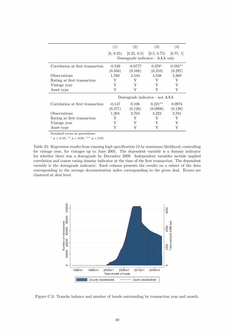
(1) (2) (3) (4)
[0, 0.25) [0.25, 0.5) [0.5, 0.75) [0.75, 1]Downgrade indicator - AAA only
Correlation at first transaction -0.539 -0.0777 0.378∗ 0.595∗∗
(0.356) (0.168) (0.210) (0.297)Observations 1,760 4,544 4,538 4,369Rating at first transaction Y Y Y YVintage year Y Y Y YAsset type Y Y Y Y
Downgrade indicator - not AAA
Correlation at first transaction -0.147 0.106 0.221∗∗ 0.0974(0.271) (0.126) (0.0908) (0.138)
Observations 1,204 2,704 4,222 2,701Rating at first transaction Y Y Y YVintage year Y Y Y YAsset type Y Y Y Y
Standard errors in parentheses∗ p < 0.10, ∗∗ p < 0.05, ∗∗∗ p < 0.01
Table 25: Regression results from running logit specification 12 by maximum likelihood, controllingfor vintage year, for vintages up to June 2005. The dependent variable is a dummy indicatorfor whether there was a downgrade by December 2009. Independent variables include impliedcorrelation and coarse rating dummy indicator at the time of the first transaction. The dependentvariable is the downgrade indicator. Each column presents the results on a subset of the datacorresponding to the average documentation index corresponding to the given deal. Errors areclustered at deal level.
Figure C.3: Tranche balance and number of bonds outstanding by transaction year and month.
49

to control for tranche-invariants such as first rating and first implied correlation. The advantage
of the panel specification 16 is that we can incorporate the partial information coming from the
late vintages (after June 2005).
outcomeit = αit + β0ρi,0 + η0ratingi0 + β1ρi,t−1 + η1ratingi,t−1 + γXi,t + εit. (13)
In equation 16 outcomeit is the month-on-month rating change in notches. Table 48 shows that
updates in signals contain information about future bond performance, but the signal is not sta-
tistically sufficient for prices. This suggests that investors retain private information over the life
of the bond, besides the information given by agency ratings. The second finding is that Alt-A
investors do not learn over the life of the bond, so that news in ratings remain statistically sufficient
for news in correlation in terms of bond performance.
To see the effect of the crisis on the information content of prices, we will use interactions with an
indicator dummy for post-2007 transaction to split estimates between before and after the crisis.
The regression specification is the following:
∆ratingit = αit + β0ρi,0 + η0ratingi0 + 1post−07 (14)
+β1ρi,t−1 × 1post−07 + η1ratingi,t−1 × 1post−07 + γXi,t + εit (15)
Table 49 presents the results of estimating equation (18). It shows that most of the effect of
news about default correlation shown in Table 48 comes from the post-crisis period. Griffin and
Nickerson (2016) discuss how rating agencies improved their methodologies following the crisis.
Under such improvement, the expectation would be that ratings become sufficient for implied
correlations, but this is not what we observe. An improvement in rating methodology is consistent
with more statistical information coming from prices if ratings are now following the market more
closely. In that case changes in implied correlation have more statistical power to predict future
downgrades by construction of the downgrade process. The other possibility is that investors
learned more from the crisis than the rating agencies, but if this is so it is rational for ratings to
follow the market more closely.
In DeMarzo (2005), two factors drive the benefits and drawbacks of securitization: private infor-
mation by the issuer, on one hand, and asset correlation, on the other. Like CDOs, CMOs are
a priori affected by it.24 Our measure of beliefs about default correlation reflects in part adverse
selection concerns on the part of the investors. Because we can’t disentangle these two components
empirically, our implied correlation measure is a proxy for market conservatism vis-a-vis informa-
tion asymmetry. In line with this, Alt-A deals being more reliant on ratings (not only for the first
transaction, but also for subsequent ones) potentially reflects a concern for asymmetric information
as in Adelino, Gerardi, and Hartman-Glaser (2016).
24Beltran et al. (2017) show that, under asymmetric information, even a modest percentage of bad securities canpush security prices far below fundamentals -even to a market meltdown-.
50

(1) (2) (3) (4)Alt-A Prime Second Lien Subprime
One-month change in rating (notches)
Lagged correlation (1 month) 0.004 0.007∗∗ -0.025∗∗∗ -0.007∗∗∗
(0.004) (0.003) (0.008) (0.003)Lagged rating (1 month) -0.026∗∗∗ -0.012∗∗∗ -0.026∗∗∗ -0.038∗∗∗
(0.001) (0.001) (0.003) (0.001)Correlation at first transaction 0.003 0.027∗∗∗ -0.004 0.008∗∗∗
(0.005) (0.003) (0.008) (0.003)Rating at first transaction 0.017∗∗∗ 0.017∗∗∗ 0.001 0.010∗∗∗
(0.001) (0.001) (0.005) (0.001)Subordination 0.084∗∗∗ 0.090∗∗∗ -0.119∗∗∗ -0.148∗∗∗
(0.022) (0.019) (0.019) (0.008)
Observations 2,032,055 1,773,020 55,293 1,452,760Vintage Y Y Y YYear-quarter Y Y Y Y
Marginal effects; Standard errors in parentheses
(d) for discrete change of dummy variable from 0 to 1∗ p < 0.10, ∗∗ p < 0.05, ∗∗∗ p < 0.01
Table 26: Regression results from running the panel regression 16, by GLS with tranche randomeffects. The first line gives the coefficient for the change over 1 month (lagged 1 month) of thecorrelation coefficient, and the second one the coefficient for the change over 1 month (lagged 1month) of the change in rating (in notches). Errors are clustered at deal level.
(1) (2) (3) (4)Alt-A Prime Second Lien Subprime
Size of downgrade (notches)
Lagged correlation -0.001 -0.018∗∗∗ 0.002 0.005(0.005) (0.004) (0.017) (0.003)
Lagged correlation × post-07=1 0.005 0.027∗∗∗ -0.028 -0.013∗∗∗
(0.006) (0.004) (0.018) (0.004)Lagged rating -0.055∗∗∗ -0.095∗∗∗ -0.082∗∗∗ -0.026∗∗∗
(0.016) (0.009) (0.014) (0.008)Lagged rating × post-07=1 0.029∗ 0.083∗∗∗ 0.056∗∗∗ -0.012
(0.016) (0.009) (0.014) (0.008)post-07=1 0.016 -0.076∗∗∗ -0.013 0.130∗∗∗
(0.019) (0.010) (0.034) (0.011)Correlation at first transaction 0.003 0.028∗∗∗ -0.001 0.008∗∗∗
(0.005) (0.003) (0.008) (0.003)Rating at first transaction 0.017∗∗∗ 0.017∗∗∗ 0.003 0.009∗∗∗
(0.001) (0.001) (0.005) (0.001)Subordination 0.084∗∗∗ 0.089∗∗∗ -0.120∗∗∗ -0.148∗∗∗
(0.022) (0.019) (0.019) (0.008)
Observations 2,032,055 1,773,020 55,293 1,452,760Vintage Y Y Y YYear-quarter Y Y Y Y
Marginal effects; Standard errors in parentheses∗ p < 0.10, ∗∗ p < 0.05, ∗∗∗ p < 0.01
Table 27: Regression results from running the panel regression 16, by GLS with tranche randomeffects. The first line gives the coefficient for the change over 1 month (lagged 1 month) of thecorrelation coefficient, and the second one the coefficient for the change over 1 month (lagged 1month) of the change in rating (in notches). Errors are clustered at deal level.
51

C.3 Additional causes of default clustering: frailty and contagion
Following Azizpour et al. (2016), defaults are driven by three factors: systemic risk25 as captured
by macroeconomic variables (Bullard et al., 2009; Khandani et al., 2013)26, an unobserved frailty
factor (Duffie et al., 2009; Kau et al., 2011) and a contagion factor, which captures the extent to
which more defaults increase the conditional intensity of default arrival.
A given loan n has a default time Tn. Defaults have a conditional mean of arrival λ given by
λt = exp
(a0 +
d∑i=1
aiXi,t
)+ Yt + Zt
where X represents a vector of macroeconomic variables. Unobservable frailty Zt follows the CIR
process
dZt = k(z − Zt)dt+ σ√ZtdWt
Z0 ∼ Γ
(2kz
σ2,σ2
2k
)Defaults are self-exciting, in the sense that the mass of defaults at a given time increases the rate
of arrival. This is captured by means of a contagion factor Y such that
Yt = b∑
n:Tn≤t
e−κ(t−Tn)Un
Un = max(0, log un)
where un is the sum of defaulted debt at time Tn. This implies that larger defaults are followed
by more defaults.
The estimation of θ = (a, k, z, σ, b, κ) is a filtered likelihood problem (the likelihood is a posterior
mean of the complete-data likelihood), and can be solved following Giesecke and Schwenkler (2016).
The likelihood is written as a product of two terms, one that depends on event data (defaults)
and one that depends on factor data. The decomposition is based on a change of measure, which
resolves the interaction between the point process and the factors of λ.27 One of the terms is
a point process filter, which makes the computation difficult. Giesecke and Schwenkler (2016)
propose an approximation based on a quadrature method, from which the posterior mean can be
computed. They write an algorithm and derive conditions for convergence.
25Bisias et al. (2012) provides a survey of systemic risk measures. See also Chan-Lau et al. (2009). Otherapproaches include macro measures (costly asset-price boom/bust cycles, property-price, equity-price, credit-gapindicators), forward-looking measures (e.g. absorption rate as in Kritzman, Li, Page, and Rigobon (2010)), cross-sectional measures (CoVaR, Co-Risk, marginal and systemic expected shortfall, see Acharya, Pedersen, Philippon,and Richardson (2012)), stress tests (e.g. Duffie (2011)), illiquidity and insolvency (e.g. Brunnermeier, Gorton, andKrishnamurthy (2011)). Giglio, Kelly, Pruitt, and Qiao (2013) use predictive quantile regression to provide anempirical assessment of 17 of them. Their main finding is that, overall, the compendium of systemic risk measurescontains useful predictive information. Instead individual measures tend to fail in capturing systematic risk.
26The characterization of systemic risk as deterioration of macroeconomic indicators leaves aside the widelydiscussed view that the pre-crisis mortgage system was systemically vulnerable (Hellwig, 2009; Poitras and Zanotti,2016).
27An alternative is to apply the expectation maximization (EM) algorithm. Giesecke and Schwenkler (2016)compare the two approaches.
52

Asset typeAfter Jun-05 Before Jun-05
Origination ($bn) Count Origination ($bn) CountAlt-A 1,179.0 16,837 557.7 11,000Prime 621.7 9,097 557.9 14,759Second Lien 64.7 478 19.0 408Subprime 660.0 9,811 720.2 9,525Total 2,525.4 36,223 1,854.8 35,692
Table 28: Issued amounts and counts by asset type.
(a) Number of tranches (b) Total issue
Figure C.4: Number of tranches and amount issued by vintage year for private label collateralizedmortgage obligations. Source: ABSNet bond data. For our sample of early vintages (prior to June2005) we provide the distribution by (coarse, see Table 42) initial rating.
Our sample Cordell et al. (2012)rating Prime/Alt-A Second Lien/Subprime Prime/Alt-A Second Lien/SubprimeAAA 10.8% 25.7% 6% 23%AA 3.4% 14.3% 3% 13%A 3.0% 5.9% 2% 8%BBB 2.9% 4.0% 1% 4%
Table 29: Subordination percentage by tranche rating - comparison. The figures computed usingABSNet data are derived by aggregating the subordination percentages at orgination as given inTable 2.4. Our sample contains only early vintages (prior to June 2005) while Cordell et al. (2012)use late vintages as well.
YearABSNet sample Adelino (2009)
Origination ($bn) Count Origination ($bn) Count≤2002 319.3 5,438
2003 470.5 10,120 496.5 8,5742004 677.4 12,519 767.3 11,4602005 904.5 16,684 1,058.5 17,1352006 1,038.0 15,022 1,080.4 18,2062007 939.4 11,716 802.1 12,037≥2008 31.2 177Total 4,380.3 71,676 4,204.8 67,412
Table 30: Origination amounts and counts at origination, by vintage year, compared to the samplein Adelino (2009).
53

Figure C.5: Average tranche price by age of the bond in months. For our sample of bonds originatedin 2004 and 2005 we compute the average price by the time elapsed (in months) since the bondissue. Vertical whiskers show the standard errors.
Figure C.6: Average subordination difference between AAA and BBB bonds. Source: ABSNetbond data.The figure presents the difference between the average AAA and average BBB subor-dination over trading time (for early vintages, prior to June 2005) using the rating at the giventrading time. The difference is computed by asset type.
54

Figure C.7: Probability of default by vintage year. We compute the default rate for each of thedeals that compose our population, and then average by vintage year and asset type. The resultsare presented here along with standard error bands around the average.
(1) (2)
Asset type Early vintages Late vintages
Alt-A 7.5% 19.5%
Prime 2.3% 6.6%
Second Lien 7.2% 25.8%
Subprime 14.8% 30.5%
Observations 4,060,698 631,793
Table 31: Liquidation rates from the loan sample. Column (1) calculates the percentage of loanslinked to early vintage deals (before June 2005) that are liquidated. Column (2) calculates thesame ratio for late vintage loans.
Figure C.8: Percentage loss given default by vintage year. The aggregate loss given default iscomputed from the sample of loans associated to the deals that compose our population of CMOs.
55

Figure C.9: Average class balance factor by asset class over tranche age. Alongside the averages, wecompute the balance factor that results from a 150% payment schedule alone (excluding plannedamortization).
Figure C.10: Standard Prepayment Model of The Bond Market Association. Prepayment percent-age for each month in the life of the underlying mortgages, expressed on an annualized basis.
56

Figure C.11: Plot of average class factor against tranche age by tranche initial rating.
downgrade(1) (2) (3)All AAA only Non-AAA only
Price -0.0187∗∗∗ -0.0457∗∗∗ -0.00932∗∗∗
(0.00151) (0.00299) (0.00149)Coupon -0.123∗∗∗ -0.0365 -0.184∗∗∗
(0.0178) (0.0245) (0.0240)Subordination -3.130∗∗∗ -3.944∗∗∗ -3.978∗∗∗
(0.268) (0.565) (0.310)
Observations 26,242 14,034 12,206Rating at first transaction Y N YVintage year Y Y Y
Standard errors in parentheses∗ p < 0.1, ∗∗ p < 0.05, ∗∗∗ p < 0.01
Table 32: Regression results from running logit regression 1 by maximum likelihood, controllingfor vintage year, for vintages up to June 2005. The dependent variable is a dummy indicator forwhether there was a downgrade by December 2009. Independent variables include price, subor-dination, coupon and coarse rating dummy indicator at the time of the first transaction. Thedependent variable is the downgrade indicator. Column (1) includes all issues; columns (2) and(3) split the sample between bonds rated AAA at origination and the rest, respectively. Errors areclustered at deal level.
57

(a) Average realized
(b) WAL
Figure C.12: Average realized and weighted average life by coarse rating and asset type. Thesecond panel includes observations where we found a matching WAL in Bloomberg.
58

Figure C.13: Proportion of ARM loans by vintage and asset type.
Figure C.14: Number of deals originated by asset type and vintage year.
59

(1) (2) (3) (4)[0, 0.25) [0.25, 0.5) [0.5, 0.75) [0.75, 1]
Downgrade indicator
Price -0.0159∗∗∗ -0.0200∗∗∗ -0.0110∗∗∗ -0.0169∗∗∗
(0.00606) (0.00333) (0.00267) (0.00354)Coupon -0.142∗∗ -0.0380 -0.117∗∗∗ -0.0780∗
(0.0640) (0.0304) (0.0441) (0.0466)Subordination 0.00163 -1.857∗∗∗ -4.016∗∗∗ -5.722∗∗∗
(0.864) (0.657) (0.489) (0.943)
Observations 2,489 5,513 7,073 5,049Rating at first transaction Y Y Y YVintage year Y Y Y YAsset type Y Y Y Y
Standard errors in parentheses∗ p < 0.10, ∗∗ p < 0.05, ∗∗∗ p < 0.01
Table 33: Regression results from running logit specification 12 by maximum likelihood, control-ling for vintage year, for vintages up to June 2005. The dependent variable is a dummy indicatorfor whether there was a downgrade by December 2009. Independent variables include price, sub-ordination, coupon and coarse rating dummy indicator at the time of the first transaction. Thedependent variable is the downgrade indicator. Each column presents the results on a subset of thedata corresponding to the average documentation index corresponding to the given deal. Errorsare clustered at deal level.
Figure C.15: Histogram plotting all outcomes from the pricing model.
60

(1) (2) (3) (4)
[0, 0.25) [0.25, 0.5) [0.5, 0.75) [0.75, 1]Downgrade indicator - AAA only
Price -0.0352∗∗∗ -0.0360∗∗∗ -0.0347∗∗∗ -0.0539∗∗∗
(0.00900) (0.00529) (0.00632) (0.0127)Coupon 0.0508∗∗∗ 0.0546 0.0919 0.118∗
(0.0161) (0.0451) (0.0575) (0.0625)Subordination -0.0174 -2.774∗∗ -2.014 -9.907∗∗∗
(1.622) (1.229) (1.881) (3.612)Observations 1,325 3,073 3,272 2,926Rating at first transaction Y Y Y YVintage year Y Y Y YAsset type Y Y Y Y
Downgrade indicator - not AAA
Price -0.0163∗∗ -0.0129∗∗∗ -0.00786∗∗∗ -0.0113∗∗∗
(0.00714) (0.00371) (0.00250) (0.00358)Coupon -0.367∗∗∗ -0.167∗∗∗ -0.201∗∗∗ -0.156∗∗∗
(0.102) (0.0475) (0.0529) (0.0603)Subordination -0.309 -2.648∗∗∗ -4.501∗∗∗ -4.193∗∗∗
(1.881) (0.880) (0.538) (0.784)Observations 1,038 2,248 3,757 2,111Rating at first transaction Y Y Y YVintage year Y Y Y YAsset type Y Y Y Y
Standard errors in parentheses∗ p < 0.10, ∗∗ p < 0.05, ∗∗∗ p < 0.01
Table 34: Regression results from running logit specification 12 by maximum likelihood, control-ling for vintage year, for vintages up to June 2005. The dependent variable is a dummy indicatorfor whether there was a downgrade by December 2009. Independent variables include price, sub-ordination, coupon and coarse rating dummy indicator at the time of the first transaction. Thedependent variable is the downgrade indicator. Each column presents the results on a subset of thedata corresponding to the average documentation index corresponding to the given deal. Errorsare clustered at deal level.
61

with data up to 2004 with data up to 2007(1) (2) (3) (4)Default Prepayment Default Prepayment
log(FICO) -1.468*** 1.408*** -2.076*** 0.305**-0.157 -0.155 -0.199 -0.12
owner occupied 0.039 -0.024 -0.098* 0.024-0.05 -0.02 -0.054 -0.02
original r - original 10 year rate 0.475*** 0.249*** 0.252*** 0.066***-0.01 -0.017 -0.011 -0.006
log(original amount) 0.421*** 0.257*** 0.143*** 0.02-0.043 -0.031 -0.041 -0.026
log(original LTV) 0.439*** -0.007 0.183*** 0.069***-0.043 -0.036 -0.033 -0.02
prepayment penalty -1.866*** -1.034*** -0.914*** -0.950***-0.08 -0.073 -0.031 -0.025
adjustable rate mortgage 0.655*** 0.493*** 0.367*** 0.467***-0.062 -0.047 -0.038 -0.015
log(Cumulative HPA) -8.398*** -7.780*** -6.482*** -2.474***-1.041 -0.963 -0.652 -0.41
coupon gap 0.400*** 0.120* -0.255*** -0.144**-0.05 -0.062 -0.04 -0.06
unemployment 0.330*** 0.320*** 0.201*** 0.319***-0.072 -0.075 -0.068 -0.075
Asset type: Prime -1.008*** -0.147*** -1.130*** -0.603***-0.078 -0.027 -0.078 -0.033
Asset type: Second Lien -0.580*** 0.124 0.843*** 0.385***-0.142 -0.079 -0.064 -0.028
Asset type: Subprime 0.504*** -0.021 1.113*** 0.201***-0.053 -0.05 -0.037 -0.02
CBSA FE Y Y Y YMonth since origination FE Y Y Y YObservations 68,634,789 76,206,672 121,236,208 126,625,633
Standard errors in parentheses∗ p < 0.1, ∗∗ p < 0.05, ∗∗∗ p < 0.01
Table 35: This table shows estimates using the maximum likelihood estimation of the complemen-tary log-log specification in (11), using a nonparametric baseline hazard, on the loan level dataavailable from ABSNet for private label loans (purchases only). The model treats competing risksindependently, indicating 1 for failure and 0 for censoring. Each coefficient is the effect of thecorresponding variable on the log hazard rate for either the default or prepayment of a mortgage.The conditional hazard is captured by performance month dummies, where performance is trackedover the first 60 months of the sample. The sample is truncated at December 2004 for columns (1)and (2), and at June 2007 for columns (3) and (4). Errors are clustered at CBSA level.
62

(1) (2)default prepayment
log(FICO) -2.481*** 0.448***-0.064 -0.018
owner occupied 0.025* 0.372***-0.014 -0.005
original r - original 10 year rate 0.429*** -0.011***-0.004 -0.001
log(original amount) 0.137*** 0.324***-0.01 -0.003
log(original LTV) 0.572*** 0.183***-0.012 -0.005
adjustable rate mortgage 0.487*** 0.579***-0.016 -0.004
log(Cumulative HPA) -1.826*** -1.581***-0.051 -0.011
coupon gap 0.848*** -0.261***-0.007 -0.002
unemployment 0.080*** 0.001-0.004 -0.001
Asset type: Prime -0.808*** -2.719***-0.044 -0.014
Asset type: Second Lien -0.794*** 0.298***-0.038 -0.011
Asset type: Subprime 0.402*** 1.079***-0.025 -0.005
CBSA FE N NMonth since origination FE N YObservations 2,630,290 76,374,400
Standard errors in parentheses∗ p < 0.1, ∗∗ p < 0.05, ∗∗∗ p < 0.01
Table 36: This table shows estimates using the maximum likelihood estimation of a complementarylog-log specification, using a hazard specification for prepayments and an dummy indicator fordefault, on the loan level data available from ABSNet for private label loans (purchases only). Thehazard model treats default risk as censored. Each coefficient is the effect of the correspondingvariable on the log hazard rate for prepayment or the log probability of default of a mortgage. Theconditional hazard is captured by performance month dummies, where performance is tracked overthe first 60 months of the sample. The sample is truncated at December 2004.
63
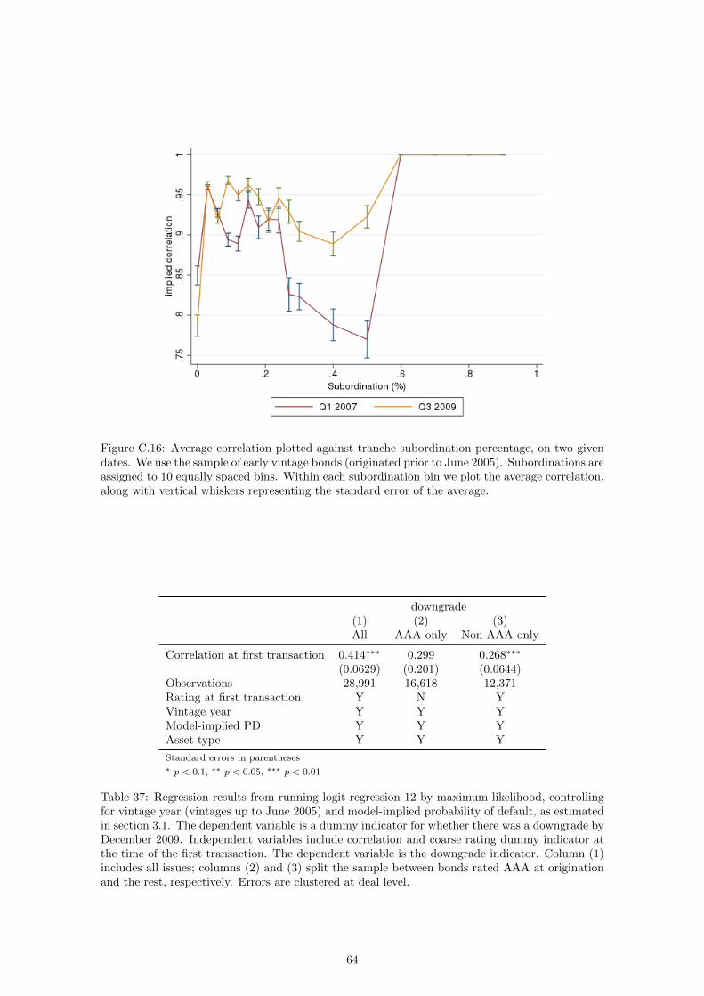
Figure C.16: Average correlation plotted against tranche subordination percentage, on two givendates. We use the sample of early vintage bonds (originated prior to June 2005). Subordinations areassigned to 10 equally spaced bins. Within each subordination bin we plot the average correlation,along with vertical whiskers representing the standard error of the average.
downgrade(1) (2) (3)All AAA only Non-AAA only
Correlation at first transaction 0.414∗∗∗ 0.299 0.268∗∗∗
(0.0629) (0.201) (0.0644)Observations 28,991 16,618 12,371Rating at first transaction Y N YVintage year Y Y YModel-implied PD Y Y YAsset type Y Y Y
Standard errors in parentheses∗ p < 0.1, ∗∗ p < 0.05, ∗∗∗ p < 0.01
Table 37: Regression results from running logit regression 12 by maximum likelihood, controllingfor vintage year (vintages up to June 2005) and model-implied probability of default, as estimatedin section 3.1. The dependent variable is a dummy indicator for whether there was a downgrade byDecember 2009. Independent variables include correlation and coarse rating dummy indicator atthe time of the first transaction. The dependent variable is the downgrade indicator. Column (1)includes all issues; columns (2) and (3) split the sample between bonds rated AAA at originationand the rest, respectively. Errors are clustered at deal level.
64

(a) Alt-A
(b) Prime
(c) Subprime
Figure C.17: Average correlation plotted against tranche subordination percentage, on two givendates. Subordination values are assigned to 10 equally spaced bins. Within each subordinationbin we plot the average correlation, along with vertical whiskers representing the standard error ofthe average.
65

(1) (2) (3) (4)[0, 0.25) [0.25, 0.5) [0.5, 0.75) [0.75, 1]
Downgrade indicator
Correlation at first transaction 0.243 0.605∗∗∗ 0.476∗∗∗ 0.569∗∗∗
(0.250) (0.200) (0.102) (0.135)Observations 2,723 6,285 7,808 5,565Rating at first transaction Y Y Y YVintage year Y Y Y YModel-implied PD Y Y Y YAsset type Y Y Y Y
Standard errors in parentheses∗ p < 0.10, ∗∗ p < 0.05, ∗∗∗ p < 0.01
Table 38: Regression results from running logit specification 12 by maximum likelihood, controllingfor vintage year (vintages up to June 2005) and model-implied probability of default as estimatedin section 3.1. The dependent variable is a dummy indicator for whether there was a downgradeby December 2009. Independent variables include implied correlation and coarse rating dummyindicator at the time of the first transaction. The dependent variable is the downgrade indica-tor. Each column presents the results on a subset of the data corresponding to the value of thedocumentation index corresponding to the given deal. Errors are clustered at deal level.
(1) (2) (3) (4)
[0, 0.25) [0.25, 0.5) [0.5, 0.75) [0.75, 1]Downgrade indicator - AAA only
Correlation at first transaction 1.018 0.430 1.647∗∗∗ 0.842∗∗∗
(0.703) (0.599) (0.627) (0.321)Observations 1,529 3,765 3,975 3,429Rating at first transaction N N N NVintage year Y Y Y YModel-implied PD Y Y Y YAsset type Y Y Y Y
Downgrade indicator - not AAA
Correlation at first transaction 0.0485 0.370∗∗ 0.314∗∗∗ 0.353∗∗
(0.283) (0.155) (0.109) (0.158)Observations 1,045 2,289 3,787 2,124Rating at first transaction Y Y Y YVintage year Y Y Y YModel-implied PD Y Y Y YAsset type Y Y Y Y
Standard errors in parentheses∗ p < 0.10, ∗∗ p < 0.05, ∗∗∗ p < 0.01
Table 39: Regression results from running logit specification 12 by maximum likelihood, controllingfor vintage year (vintages up to June 2005) and model-implied probability of default as estimatedin section 3.1. The dependent variable is a dummy indicator for whether there was a downgradeby December 2009. Independent variables include implied correlation and coarse rating dummyindicator at the time of the first transaction. The dependent variable is the downgrade indica-tor. Each column presents the results on a subset of the data corresponding to the value of thedocumentation index corresponding to the given deal. Errors are clustered at deal level.
66

(1) (2) (3) (4)AAA balance at origination as share of deal issuance
Opacity index -0.104∗∗∗ -0.0835∗∗∗ -0.101∗∗∗ -0.0259∗
(0.0154) (0.0153) (0.0151) (0.0151)
Observations 1,902 1,902 1,902 1,902Model-implied PD N Y Y YVintage year N N Y YAsset type N N N Y
Standard errors in parentheses∗ p < 0.10, ∗∗ p < 0.05, ∗∗∗ p < 0.01
Table 40: Regression results from running a linear regression at deal level of AAA origination (asshare of total) on the deal opacity index. Controls include model-implied PD, vintage year (weinclude vintages up to June 2005) and asset type.
D Data cleaning
E Bond data
We start with 16,397,826 panel observations, corresponding to 127,963 tranches. I remove data
entry errors such as subordination percentages larger than one. In those cases all observations for
the month (all tranches linked to the deal involved) are removed so as to ensure computations of the
tranching structure are correct.28 We follow Adelino (2009) in removing Interest Only, Principal
Only, Inverse Floater and Fixed to Variable bonds from the sample.
Stage Tranches leftRemove deals that are entirely made of mixed asset types 119,215Remove deals where one tranche has subordination >1 119,215Remove observations with missing price 74,307Remove mixed-type asset pools 74,253Remove PO, IO, IF and FtV 71,950
Table 41: Data cleaning stages with number of tranches outstanding at the end of each step.
Notice that the most aggressive cleaning step is the removal of observations where price is missing.
As dicussed in section 2, this is due to the data gap that covers late (2005 and more recent)
vintages.
F Loan level data
We start with a set of 22,008,610 loan originations. Of our originations set, 21,759,836 map to one
of our deal IDs. Below is a summary of deal level averages of certain covariates (FICO score, LTV,
private mortgage insurance coverage percentage) are computed.29
28I manually computed subordination percentages on a random sample of deals to check the calculations byABSNet.
29Simple averages were preferred over weighted averages (weighted by e.g. the initial securitized balance) as thisreduces the number of missing observations.
67

S&P rating Code Coarse rating CodeAAA 1 AAA 1AA+ 2 AA 2AA 3 AA 2AA- 4 AA 2A+ 5 A 3A 6 A 3A- 7 A 3BBB+ 8 BBB 4BBB 9 BBB 4BBB- 10 BBB 4BB+ 11 BB 5BB 12 BB 5BB- 13 BB 5B+ 14 B 6B 15 B 6B- 16 B 6CCC 17 C 7CCC- 18 C 7CC 19 C 7C 20 C 7D 21 D 8NR - NR -
Table 42: Mapping of ratings - fine and coarse level (with numbering code)
(a) FICO score (b) PMI coverage
Figure F.1: Distribution of covariates over time (vintage year).
68
(a) LTV (b) Original securitized balance
Figure F.2: Distribution of covariates over time (vintage year).
Historic data are contained in monthly reports. From the input 21,996,382 facilities we have at least
one observation for 17,350,072 of them. We recover a total 792,664,139 loan-month observations
from payment history (on average 45.7 obs per loan). From there we can compute default rates
at deal level. We have loss event data for 3,986,974 observations, linked to 5,965 deal IDs. From
there we can compute LGDs at deal level or vintage level.
At the loan level, we keep only loans having purchase as purpose. This reduces the sample to
8,862,561 loans. Aside minor cleaning (originations before 1980, errors in time stamps) we arrive
to 7,145,251. From these we discard asset types other than Alt-A, Prime, Second Lien or Subprime
to arrive at the initial sample composed of early and late vintages.
G Variations on the baseline model
H Pricing results with constant default probability and pre-
payment speed
In this section we use a constant PD, by asset type, given as the
After the collapse of private label securitization in 2007, most securitization conduits are insured
against default risk by the Government-Sponsored Entities (Fannie Mae and Freddie Mac), mak-
ing prepayment risk the most significant one in the literature. Schwartz and Torous (1989) and
Stanton (1995) measure the value of prepayment option in default-free securities (guaranteed by
the Government-Sponsored Entities). Downing et al. (2005) propose a two-factor valuation model
that distinguishes the separate, competing risks carried by the default and the prepayment options.
Sugimura (2004) develops an intensity model to price RMBS (pass-through) bonds not insured
against default risk, and thus exposed to both prepayment and default risk (but credit events in
69

(1) (2) (3)
Asset type Early vintages Late vintages Model PD
Alt-A 7.5% 19.5% 24.5%
Prime 2.3% 6.6% 6.4%
Second Lien 7.2% 25.8% 21.1%
Subprime 14.8% 30.5% 30%
Observations 4,060,698 631,793 2,112
Table 43: Liquidation rates from the loan sample, and PD used for baseline estimation. Column(1) calculates the percentage of loans linked to early vintage deals (before June 2005) that areliquidated. Column (2) calculates the same ratio for late vintage loans. Column (3) shows the PDparameters used for the pricing model, calculated as the average of the deal level liquidation ratesfor both early and late deals.
his approach are assumed to be uncorrelated). We seek an accurate measure of prepayment while
keeping the focus on default risk, hence the choice of the PSA schedule (see Figure C.10).
In order to chose the PSA factor we look at the class balance. Class balance factor, which measures
balance over time relative to the tranche initial balance, reflects both losses and prepayments,
thus is an upper bound for prepayments. The results in Figure C.9 suggest that 150% is an
appropriate upper bound. Gorton (2009) states that subprime deals were mostly linked to ARMs
(see Figure C.13), those being a priori subject to higher prepayment rates.30 The evolution of
class factor over time does not suggest a radically different prepayment rate for subprime deals in
our sample. In this section we will apply the PSA schedule, with a factor of 150%, to all tranches
within the same deal.
Cornaggia et al. (2017) find that ratings are not comparable across broad asset types (corporate,
CDO, ABS and RMBS). Within RMBS we emphasize the difference across asset types (prime,
subprime and Alt-A), and in this section document a difference in information across asset types,
namely between Alt-A and other types.
Breaking the change by asset type we see an increase for Alt-A tranches (from 0.36 to 0.40), no
change for prime ones (0.30) and a decrease for subprime deals (from 0.59 to 0.49, significant at
99%) so that the upward adjustment during seems to have mainly affected Alt-A issues.
In terms of seniorities, the difference observed by Buzkova and Teply (2012) over the crisis is mainly
driven by mezzanine tranches (7%-10% and 10%-15%). Figure H.1 also suggests the increase in
correlations is larger among intermediate seniorities, though not as large as the one they observe
on the CDX tranches. We now look at average correlation over time (see Figure H.2).
The regression results on price informativeness are similar to those obtained in Section 4: implied
default correlations are informative when they are linked to well-documented deals, which happens
both for AAA and non-AAA tranches. First, the results in Table 44 confirm those of Table 37
in that implied correlations are informative about bond downgrades, except for AAA tranches.
Second, the split by opacity index (see Table 46) yields a similar results to that in Table 38.
30He finds that the shift to subprime deals happened for the later cohorts. Similarly, we find that later cohortssee faster reductions in balance.
70

Figure H.1: Average correlation plotted against tranche subordination percentage, on two givendates. We use the sample of early vintage bonds (originated prior to June 2005). Subordinations areassigned to 10 equally spaced bins. Within each subordination bin we plot the average correlation,along with vertical whiskers representing the standard error of the average.
Finally, the further split by rating in Table 46 yields results that are consistent with those in
Table 38.
I The information content of news in prices
Using the partial observations we recover from the ABSNet data (namely, observations post June
2009) we study the effect of news in prices across the cycle. A number of cleaning stages (see
Table 41 in the appendix) are applied to attain the final sample, which contains 6,322,690 panel
observations -close to 64 transactions per tranche-. We illustrate the overall numbers in Figure I.1.
The results up to now suggest implied correlation at origination is predictive of downgrades to the
extent that the loans have full documentation. Having seen the role of initial signals, our next
question is about the role of price news both from rating agencies and the market. While initial
ratings rely on an a priori assessment, its evolution over time reflects progressively more of the
bond performance, implying that updated rating values should in principle absorb the information
that was initially private. We estimate panel 16 using a linear model, with random effects in order
to control for tranche-invariants such as first rating and first implied correlation. The advantage
of the panel specification 16 is that we can incorporate the partial information coming from the
late vintages (after June 2005).
outcomeit = αit + β0ρi,0 + η0ratingi0 + β1ρi,t−1 + η1ratingi,t−1 + γXi,t + εit. (16)
71

(a) Implied correlation - Alt-A (b) Rating - Alt-A
(c) Implied correlation - prime (d) Rating - prime
(e) Implied correlation - subprime (f) Rating - subprime
Figure H.2: Performance of early vintage tranches: average implied correlation and average rat-ing for bonds originated before June 2005. For a given we compute the implied correlation, ateach point in time. The average is taken by transaction period, by coarse rating at origination(AAA=1,..., BBB=4,..., D=8).
72
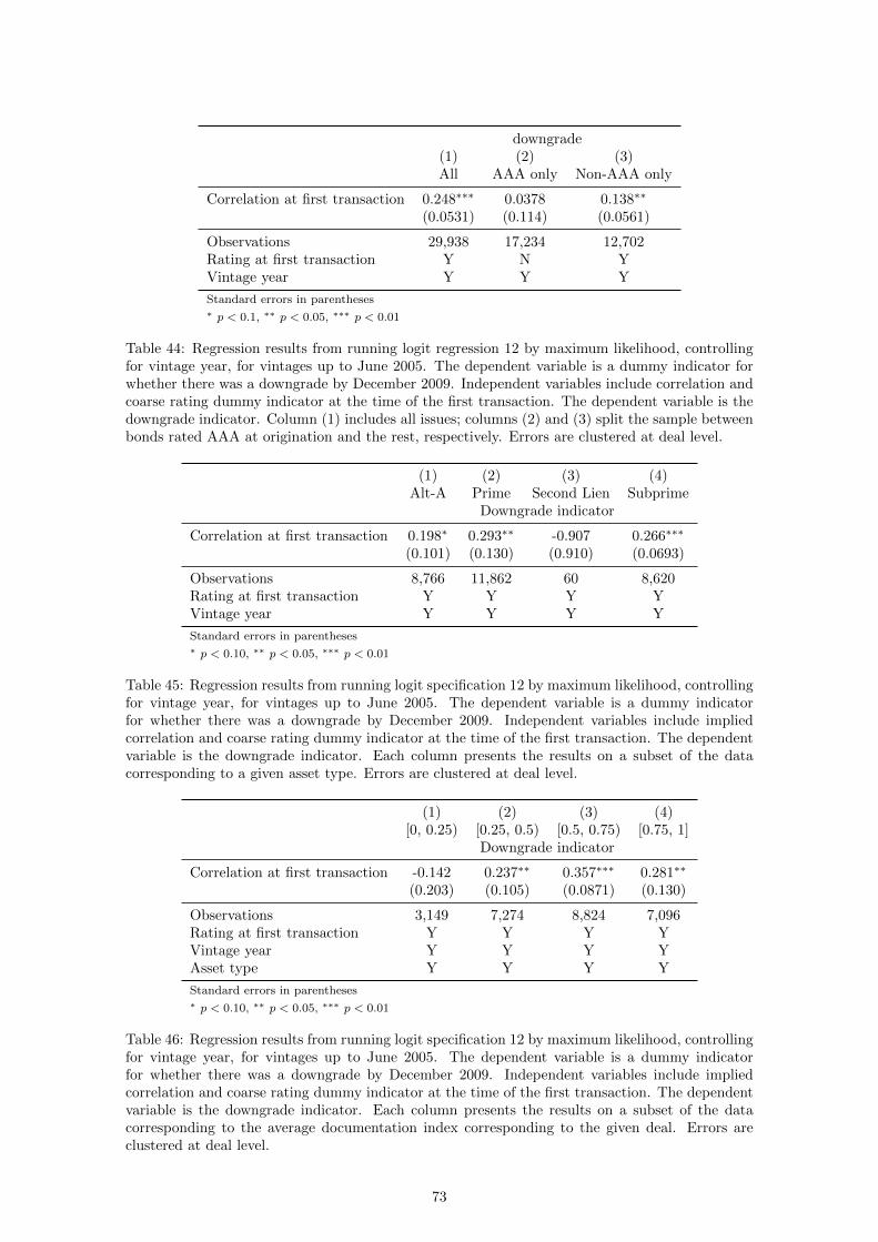
downgrade(1) (2) (3)All AAA only Non-AAA only
Correlation at first transaction 0.248∗∗∗ 0.0378 0.138∗∗
(0.0531) (0.114) (0.0561)
Observations 29,938 17,234 12,702Rating at first transaction Y N YVintage year Y Y Y
Standard errors in parentheses∗ p < 0.1, ∗∗ p < 0.05, ∗∗∗ p < 0.01
Table 44: Regression results from running logit regression 12 by maximum likelihood, controllingfor vintage year, for vintages up to June 2005. The dependent variable is a dummy indicator forwhether there was a downgrade by December 2009. Independent variables include correlation andcoarse rating dummy indicator at the time of the first transaction. The dependent variable is thedowngrade indicator. Column (1) includes all issues; columns (2) and (3) split the sample betweenbonds rated AAA at origination and the rest, respectively. Errors are clustered at deal level.
(1) (2) (3) (4)Alt-A Prime Second Lien Subprime
Downgrade indicator
Correlation at first transaction 0.198∗ 0.293∗∗ -0.907 0.266∗∗∗
(0.101) (0.130) (0.910) (0.0693)
Observations 8,766 11,862 60 8,620Rating at first transaction Y Y Y YVintage year Y Y Y Y
Standard errors in parentheses∗ p < 0.10, ∗∗ p < 0.05, ∗∗∗ p < 0.01
Table 45: Regression results from running logit specification 12 by maximum likelihood, controllingfor vintage year, for vintages up to June 2005. The dependent variable is a dummy indicatorfor whether there was a downgrade by December 2009. Independent variables include impliedcorrelation and coarse rating dummy indicator at the time of the first transaction. The dependentvariable is the downgrade indicator. Each column presents the results on a subset of the datacorresponding to a given asset type. Errors are clustered at deal level.
(1) (2) (3) (4)[0, 0.25) [0.25, 0.5) [0.5, 0.75) [0.75, 1]
Downgrade indicator
Correlation at first transaction -0.142 0.237∗∗ 0.357∗∗∗ 0.281∗∗
(0.203) (0.105) (0.0871) (0.130)
Observations 3,149 7,274 8,824 7,096Rating at first transaction Y Y Y YVintage year Y Y Y YAsset type Y Y Y Y
Standard errors in parentheses∗ p < 0.10, ∗∗ p < 0.05, ∗∗∗ p < 0.01
Table 46: Regression results from running logit specification 12 by maximum likelihood, controllingfor vintage year, for vintages up to June 2005. The dependent variable is a dummy indicatorfor whether there was a downgrade by December 2009. Independent variables include impliedcorrelation and coarse rating dummy indicator at the time of the first transaction. The dependentvariable is the downgrade indicator. Each column presents the results on a subset of the datacorresponding to the average documentation index corresponding to the given deal. Errors areclustered at deal level.
73

(1) (2) (3) (4)
[0, 0.25) [0.25, 0.5) [0.5, 0.75) [0.75, 1]Downgrade indicator - AAA only
Correlation at first transaction -0.539 -0.0777 0.378∗ 0.595∗∗
(0.356) (0.168) (0.210) (0.297)Observations 1,760 4,544 4,538 4,369Rating at first transaction Y Y Y YVintage year Y Y Y YAsset type Y Y Y Y
Downgrade indicator - not AAA
Correlation at first transaction -0.147 0.106 0.221∗∗ 0.0974(0.271) (0.126) (0.0908) (0.138)
Observations 1,204 2,704 4,222 2,701Rating at first transaction Y Y Y YVintage year Y Y Y YAsset type Y Y Y Y
Standard errors in parentheses∗ p < 0.10, ∗∗ p < 0.05, ∗∗∗ p < 0.01
Table 47: Regression results from running logit specification 12 by maximum likelihood, controllingfor vintage year, for vintages up to June 2005. The dependent variable is a dummy indicatorfor whether there was a downgrade by December 2009. Independent variables include impliedcorrelation and coarse rating dummy indicator at the time of the first transaction. The dependentvariable is the downgrade indicator. Each column presents the results on a subset of the datacorresponding to the average documentation index corresponding to the given deal. Errors areclustered at deal level.
Figure I.1: Tranche balance and number of bonds outstanding by transaction year and month.
74
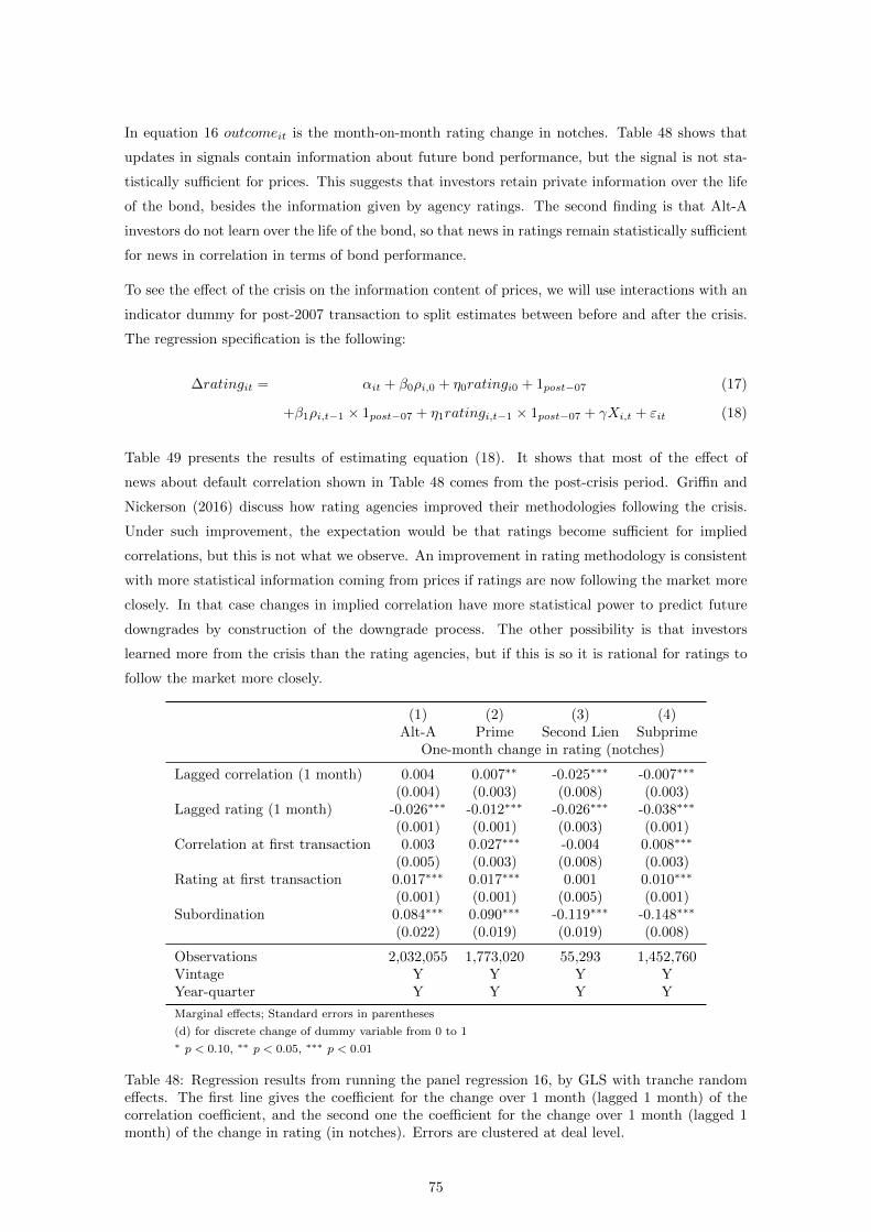
In equation 16 outcomeit is the month-on-month rating change in notches. Table 48 shows that
updates in signals contain information about future bond performance, but the signal is not sta-
tistically sufficient for prices. This suggests that investors retain private information over the life
of the bond, besides the information given by agency ratings. The second finding is that Alt-A
investors do not learn over the life of the bond, so that news in ratings remain statistically sufficient
for news in correlation in terms of bond performance.
To see the effect of the crisis on the information content of prices, we will use interactions with an
indicator dummy for post-2007 transaction to split estimates between before and after the crisis.
The regression specification is the following:
∆ratingit = αit + β0ρi,0 + η0ratingi0 + 1post−07 (17)
+β1ρi,t−1 × 1post−07 + η1ratingi,t−1 × 1post−07 + γXi,t + εit (18)
Table 49 presents the results of estimating equation (18). It shows that most of the effect of
news about default correlation shown in Table 48 comes from the post-crisis period. Griffin and
Nickerson (2016) discuss how rating agencies improved their methodologies following the crisis.
Under such improvement, the expectation would be that ratings become sufficient for implied
correlations, but this is not what we observe. An improvement in rating methodology is consistent
with more statistical information coming from prices if ratings are now following the market more
closely. In that case changes in implied correlation have more statistical power to predict future
downgrades by construction of the downgrade process. The other possibility is that investors
learned more from the crisis than the rating agencies, but if this is so it is rational for ratings to
follow the market more closely.
(1) (2) (3) (4)Alt-A Prime Second Lien Subprime
One-month change in rating (notches)
Lagged correlation (1 month) 0.004 0.007∗∗ -0.025∗∗∗ -0.007∗∗∗
(0.004) (0.003) (0.008) (0.003)Lagged rating (1 month) -0.026∗∗∗ -0.012∗∗∗ -0.026∗∗∗ -0.038∗∗∗
(0.001) (0.001) (0.003) (0.001)Correlation at first transaction 0.003 0.027∗∗∗ -0.004 0.008∗∗∗
(0.005) (0.003) (0.008) (0.003)Rating at first transaction 0.017∗∗∗ 0.017∗∗∗ 0.001 0.010∗∗∗
(0.001) (0.001) (0.005) (0.001)Subordination 0.084∗∗∗ 0.090∗∗∗ -0.119∗∗∗ -0.148∗∗∗
(0.022) (0.019) (0.019) (0.008)
Observations 2,032,055 1,773,020 55,293 1,452,760Vintage Y Y Y YYear-quarter Y Y Y Y
Marginal effects; Standard errors in parentheses
(d) for discrete change of dummy variable from 0 to 1∗ p < 0.10, ∗∗ p < 0.05, ∗∗∗ p < 0.01
Table 48: Regression results from running the panel regression 16, by GLS with tranche randomeffects. The first line gives the coefficient for the change over 1 month (lagged 1 month) of thecorrelation coefficient, and the second one the coefficient for the change over 1 month (lagged 1month) of the change in rating (in notches). Errors are clustered at deal level.
75

(1) (2) (3) (4)Alt-A Prime Second Lien Subprime
Size of downgrade (notches)
Lagged correlation -0.001 -0.018∗∗∗ 0.002 0.005(0.005) (0.004) (0.017) (0.003)
Lagged correlation × post-07=1 0.005 0.027∗∗∗ -0.028 -0.013∗∗∗
(0.006) (0.004) (0.018) (0.004)Lagged rating -0.055∗∗∗ -0.095∗∗∗ -0.082∗∗∗ -0.026∗∗∗
(0.016) (0.009) (0.014) (0.008)Lagged rating × post-07=1 0.029∗ 0.083∗∗∗ 0.056∗∗∗ -0.012
(0.016) (0.009) (0.014) (0.008)post-07=1 0.016 -0.076∗∗∗ -0.013 0.130∗∗∗
(0.019) (0.010) (0.034) (0.011)Correlation at first transaction 0.003 0.028∗∗∗ -0.001 0.008∗∗∗
(0.005) (0.003) (0.008) (0.003)Rating at first transaction 0.017∗∗∗ 0.017∗∗∗ 0.003 0.009∗∗∗
(0.001) (0.001) (0.005) (0.001)Subordination 0.084∗∗∗ 0.089∗∗∗ -0.120∗∗∗ -0.148∗∗∗
(0.022) (0.019) (0.019) (0.008)
Observations 2,032,055 1,773,020 55,293 1,452,760Vintage Y Y Y YYear-quarter Y Y Y Y
Marginal effects; Standard errors in parentheses∗ p < 0.10, ∗∗ p < 0.05, ∗∗∗ p < 0.01
Table 49: Regression results from running the panel regression 16, by GLS with tranche randomeffects. The first line gives the coefficient for the change over 1 month (lagged 1 month) of thecorrelation coefficient, and the second one the coefficient for the change over 1 month (lagged 1month) of the change in rating (in notches). Errors are clustered at deal level.
76

In DeMarzo (2005), two factors drive the benefits and drawbacks of securitization: private infor-
mation by the issuer, on one hand, and asset correlation, on the other. Like CDOs, CMOs are
a priori affected by it.31 Our measure of beliefs about default correlation reflects in part adverse
selection concerns on the part of the investors. Because we can’t disentangle these two components
empirically, our implied correlation measure is a proxy for market conservatism vis-a-vis informa-
tion asymmetry. In line with this, Alt-A deals being more reliant on ratings (not only for the first
transaction, but also for subsequent ones) potentially reflects a concern for asymmetric information
as in Adelino et al. (2016).
J Additional causes of default clustering: frailty and conta-
gion
Following Azizpour et al. (2016), defaults are driven by three factors: systemic risk32 as captured
by macroeconomic variables (Bullard et al., 2009; Khandani et al., 2013)33, an unobserved frailty
factor (Duffie et al., 2009; Kau et al., 2011) and a contagion factor, which captures the extent to
which more defaults increase the conditional intensity of default arrival.
A given loan n has a default time Tn. Defaults have a conditional mean of arrival λ given by
λt = exp
(a0 +
d∑i=1
aiXi,t
)+ Yt + Zt
where X represents a vector of macroeconomic variables. Unobservable frailty Zt follows the CIR
process
dZt = k(z − Zt)dt+ σ√ZtdWt
Z0 ∼ Γ
(2kz
σ2,σ2
2k
)Defaults are self-exciting, in the sense that the mass of defaults at a given time increases the rate
of arrival. This is captured by means of a contagion factor Y such that
Yt = b∑
n:Tn≤t
e−κ(t−Tn)Un
Un = max(0, log un)
31Beltran et al. (2017) show that, under asymmetric information, even a modest percentage of bad securities canpush security prices far below fundamentals -even to a market meltdown-.
32Bisias et al. (2012) provides a survey of systemic risk measures. See also Chan-Lau et al. (2009). Otherapproaches include macro measures (costly asset-price boom/bust cycles, property-price, equity-price, credit-gapindicators), forward-looking measures (e.g. absorption rate as in Kritzman et al. (2010)), cross-sectional measures(CoVaR, Co-Risk, marginal and systemic expected shortfall, see Acharya et al. (2012)), stress tests (e.g. Duffie(2011)), illiquidity and insolvency (e.g. Brunnermeier et al. (2011)). Giglio et al. (2013) use predictive quantileregression to provide an empirical assessment of 17 of them. Their main finding is that, overall, the compendium ofsystemic risk measures contains useful predictive information. Instead individual measures tend to fail in capturingsystematic risk.
33The characterization of systemic risk as deterioration of macroeconomic indicators leaves aside the widelydiscussed view that the pre-crisis mortgage system was systemically vulnerable (Hellwig, 2009; Poitras and Zanotti,2016).
77

where un is the sum of defaulted debt at time Tn. This implies that larger defaults are followed
by more defaults.
The estimation of θ = (a, k, z, σ, b, κ) is a filtered likelihood problem (the likelihood is a posterior
mean of the complete-data likelihood), and can be solved following Giesecke and Schwenkler (2016).
The likelihood is written as a product of two terms, one that depends on event data (defaults)
and one that depends on factor data. The decomposition is based on a change of measure, which
resolves the interaction between the point process and the factors of λ.34 One of the terms is
a point process filter, which makes the computation difficult. Giesecke and Schwenkler (2016)
propose an approximation based on a quadrature method, from which the posterior mean can be
computed. They write an algorithm and derive conditions for convergence.
34An alternative is to apply the expectation maximization (EM) algorithm. Giesecke and Schwenkler (2016)compare the two approaches.
78

References
Acharya, V. V., L. H. Pedersen, T. Philippon, and M. P. Richardson (2012, Feb). Measuring
systemic risk.
Adelino, M. (2009). Do investors rely only on ratings? the case of mortgage-backed securities.
Adelino, M., K. Gerardi, and B. Hartman-Glaser (2016). Are lemons sold first? dynamic signaling
in the mortgage market.
Altman, E. I. (2006). Default recovery rates and lgd in credit risk modeling and practice: an
updated review of the literature and empirical evidence. New York University, Stern School of
Business.
Andersen, L. and J. Sidenius (2004). Extensions to the gaussian copula: Random recovery and
random factor loadings. Journal of Credit Risk 1 (1), 05.
Andreoli, A., L. V. Ballestra, and G. Pacelli (2016). From insurance risk to credit portfolio
management: a new approach to pricing CDOs. Quantitative Finance 16 (10), 1495–1510.
Ashcraft, A., P. Goldsmith-Pinkham, P. Hull, and J. Vickery (2011). Credit ratings and security
prices in the subprime mbs market. The American Economic Review 101 (3), 115–119.
Ashcraft, A., P. Goldsmith-Pinkham, and J. Vickery (2010). Mbs ratings and the mortgage credit
boom.
Ashcraft, A. B. and T. Schuermann (2008). Understanding the securitization of subprime mortgage
credit. Foundations and Trends R© in Finance 2 (3), 191–309.
Azizpour, S., K. Giesecke, and G. Schwenkler (2016). Exploring the sources of default clustering.
Bai, J., P. Collin-Dufresne, R. S. Goldstein, and J. Helwege (2015). On bounding credit-event risk
premia. The Review of Financial Studies 28 (9), 2608.
Beltran, D. O., L. Cordell, and C. P. Thomas (2017). Asymmetric information and the death of
ABS CDOs. Journal of Banking & Finance 76, 1 – 14.
Benesova, P. and P. Teply (2010, January). Main Flaws of The Collateralized Debt Obligation?s:
Valuation Before And During The 2008/2009 Global Turmoil. Working Papers IES 2010/01,
Charles University Prague, Faculty of Social Sciences, Institute of Economic Studies.
Benmelech, E. and J. Dlugosz (2010). The credit rating crisis. NBER Macroeconomics An-
nual 24 (1), 161–208.
Berndt, A., R. Douglas, D. Duffie, M. Ferguson, and D. Schranz (2005). Measuring default risk
premia from default swap rates and edfs.
Bisias, D., M. Flood, A. W. Lo, and S. Valavanis (2012). A survey of systemic risk analytics.
Annual Review of Financial Economics 4 (1), 255–296.
Brunne, T. (2006). Implied correlation of synthetic CDOs with liquid markets.
79

Brunnermeier, M. K., G. Gorton, and A. Krishnamurthy (2011). Risk Topography, pp. 149–176.
National Bureau of Economic Research, Inc.
Bullard, J., C. J. Neely, D. C. Wheelock, et al. (2009). Systemic risk and the financial crisis: a
primer. Federal Reserve Bank of St. Louis Review 91 (5 Part 1), 403–18.
Buzkova, P. and P. Teply (2012). Collateralized debt obligations valuation using the one factor
gaussian copula model. Prague Economic Papers 21 (1), 30–49.
Carlin, B. I., F. A. Longstaff, and K. Matoba (2014). Disagreement and asset prices. Journal of
Financial Economics 114 (2), 226 – 238.
Chan-Lau, J. A., M. Espinosa, K. Giesecke, and J. A. Sole (2009). Assessing the systemic impli-
cations of financial linkages. IMF Global Financial Stability Report 2.
Cordell, L., Y. Huang, and M. Williams (2012). Collateral damage: Sizing and assessing the
subprime CDO crisis.
Cornaggia, J. N., K. J. Cornaggia, and J. E. Hund (2017). Credit ratings across asset classes: A
long-term perspective*. Review of Finance 21 (2), 465–509.
Coval, J., J. Jurek, and E. Stafford (2009a). The economics of structured finance. The Journal of
Economic Perspectives 23 (1), 3–25.
Coval, J. D., J. W. Jurek, and E. Stafford (2009b). Economic catastrophe bonds. The American
Economic Review 99 (3), 628–666.
Cowan, A. M. and C. D. Cowan (2004). Default correlation: An empirical investigation of a sub-
prime lender. Journal of Banking & Finance 28 (4), 753 – 771. Retail Credit Risk Management
and Measurement.
Crouhy, M., D. Galai, and R. Mark (2000). A comparative analysis of current credit risk models.
Journal of Banking & Finance 24 (1), 59–117.
D’Amato, J. and J. Gyntelberg (2005). CDS index tranches and the pricing of credit risk correla-
tions. BIS Quarterly Review .
Dang, T. V., G. Gorton, and B. Holmstrom (2013). The information sensitivity of a security.
Unpublished working paper, Yale University .
de Servigny, A. and O. Renault (2002). Default correlation: empirical evidence. Standard and
Poor’s.
Dell’Ariccia, G., D. Igan, and L. Laeven (2012, 03). Credit Booms and Lending Standards: Evi-
dence from the Subprime Mortgage Market. Journal of Money, Credit and Banking 44, 367–384.
DeMarzo, P. M. (2005). The pooling and tranching of securities: A model of informed intermedi-
ation. Review of Financial Studies 18 (1), 1–35.
80

Deng, Y., S. A. Gabriel, and A. B. Sanders (2011). CDO market implosion and the pricing of
subprime mortgage-backed securities. Journal of Housing Economics 20 (2), 68 – 80. Special
Issue: Housing and the Credit Crunch.
Denzler, S. M., M. M. Dacorogna, U. A. Muller, and A. J. McNeil (2006). From default probabilities
to credit spreads: Credit risk models do explain market prices. Finance Research Letters 3 (2),
79–95.
Diep, P., A. L. Eisfeldt, and S. A. Richardson (2016). Prepayment risk and expected mbs returns.
Downing, C., R. Stanton, and N. Wallace (2005). An empirical test of a two-factor mortgage
valuation model: How much do house prices matter? Real Estate Economics 33 (4), 681–710.
Duffie, D. (2008, July). Innovations in credit risk transfer: Implications for financial stability. BIS
Working Paper (255).
Duffie, D. (2011, August 2011). Systemic risk exposures: A 10-by-10-by-10 approach. National
Bureau of Economic Research Working Paper Series No. 17281.
Duffie, D., A. Eckner, G. Horel, and L. Saita (2009). Frailty correlated default. The Journal of
Finance 64 (5), 2089–2123.
Duffie, D. and N. Garleanu (2001). Risk and valuation of collateralized debt obligations. Financial
Analysts Journal 57 (1), 41–59.
Duffie, D. and K. J. Singleton (2012). Credit risk: pricing, measurement, and management. Prince-
ton University Press.
Elizalde, A. (2005). Credit risk models iv: Understanding and pricing cdos. CEMFI and Univer-
sidad Publica de Navarro, download: www. cemfi. es/ elizalde.
Frye, J. (2008). Correlation and asset correlation in the structural portfolio model. The Journal
of Credit Risk 4 (2), 75–96.
Geidosh, M. (2014, 06). Asset correlation in residential mortgage-backed security reference port-
folios. Journal of Credit Risk 10 (2), 71–95.
Giesecke, K. and G. Schwenkler (2016). Filtered likelihood for point processes.
Giglio, S., B. Kelly, S. Pruitt, and X. Qiao (2013). Systemic risk and the macroeconomy: An
empirical evaluation. Chicago Booth Research Paper (12-49).
Gordy, M. B. (2000). A comparative anatomy of credit risk models. Journal of Banking &
Finance 24 (1), 119–149.
Gorton, G. (2009). The subprime panic*. European Financial Management 15 (1), 10–46.
Gorton, G. B. and G. Ordonez (2013). The supply and demand for safe assets. Technical report,
National Bureau of Economic Research.
Griffin, J. M. and J. Nickerson (2016). Debt correlations in the wake of the financial crisis: What
are appropriate default correlations for structured products?
81

Griffin, J. M. and D. Y. Tang (2012). Did subjectivity play a role in cdo credit ratings? The
Journal of Finance 67 (4), 1293–1328.
Gupta, A. (2016). Foreclosure contagion and the neighborhood spillover effects of mortgage de-
faults. Technical report, Working Paper.
Hellwig, M. F. (2009). Systemic risk in the financial sector: An analysis of the subprime-mortgage
financial crisis. De Economist 157 (2), 129–207.
Heynderickx, W., J. Cariboni, W. Schoutens, and B. Smits (2016). The relationship between risk-
neutral and actual default probabilities: the credit risk premium. Applied Economics 48 (42),
4066–4081.
Hull, J. and A. White (2008). Dynamic models of portfolio credit risk: A simplified approach.
Journal of Derivatives 15 (4), 9–28.
Hull, J. C. and A. D. White (2004). Valuation of a CDO and an n-th to default CDS without
monte carlo simulation. The Journal of Derivatives 12 (2), 8–23.
Hull, J. C. and A. D. White (2006). Valuing credit derivatives using an implied copula approach.
The Journal of Derivatives 14 (2), 8–28.
IOSCO (2008, March). The role of credit rating agencies in structured finance markets. Technical
report, International Organization of Securities Commissions.
Jarrow, R. A. (2011). Risk management models: construction, testing, usage. The Journal of
Derivatives 18 (4), 89–98.
JEC (2007). The subprime lending crisis: The economic impact on wealth, property values
and tax revenues, and how we got here. World Wide Web page¡ http://www. jec. senate.
gov/Documents/Reports/10.25. 07OctoberSubprimeReport. pdf¿(accessed January 15, 2008).
Kau, J. B., D. C. Keenan, and X. Li (2011). An analysis of mortgage termination risks: a
shared frailty approach with msa-level random effects. The Journal of Real Estate Finance
and Economics 42 (1), 51–67.
Kau, J. B., D. C. Keenan, C. Lyubimov, and V. C. Slawson (2011). Subprime mortgage default.
Journal of Urban Economics 70 (2), 75–87.
Keys, B. J., T. Mukherjee, A. Seru, and V. Vig (2010). Did securitization lead to lax screening?
evidence from subprime loans. The Quarterly journal of economics 125 (1), 307–362.
Khandani, A. E., A. W. Lo, and R. C. Merton (2013). Systemic risk and the refinancing ratchet
effect. Journal of Financial Economics 108 (1), 29–45.
Kritzman, M., Y. Li, S. Page, and R. Rigobon (2010). Principal components as a measure of
systemic risk.
Li, D. X. (2000). On default correlation: A copula function approach. The Journal of Fixed
Income 9 (4), 43–54.
82

Liu, H. (2016). Do government guarantees inhibit risk management? evidence from Fannie Mae
and Freddie Mac.
Longstaff, F. A. and A. Rajan (2008). An empirical analysis of the pricing of collateralized debt
obligations. The Journal of Finance 63 (2), 529–563.
McGinty, L., E. Beinstein, R. Ahluwalia, and M. Watts (2004). Credit correlation: A guide.
Technical report.
Nagpal, K. and R. Bahar (2001). Measuring default correlation. Risk 14 (3), 129–132.
O’Kane, D. and M. Livesey (2004). Base correlation explained. Lehman Brothers, Fixed Income
Quantitative Credit Research.
Palmer, C. (2015). Why did so many subprime borrowers default during the crisis: Loose credit
or plummeting prices?
Poitras, G. and G. Zanotti (2016). Mortgage contract design and systemic risk immunization.
International Review of Financial Analysis 45, 320–331.
Rapisarda, G. and D. Echeverry (2013). A nonparametric approach to incorporating incomplete
workouts into loss given default estimates. The Journal of Credit Risk 9 (2), 47.
Schlosser, A. (2011). Pricing and risk management of synthetic CDOs, Volume 646. Springer
Science & Business Media.
Schwartz, E. S. and W. N. Torous (1989). Prepayment and the valuation of mortgage-backed
securities. The Journal of Finance 44 (2), 375–392.
Simsek, A. (2013). Belief disagreements and collateral constraints. Econometrica 81 (1), 1–53.
Sirignano, J., A. Sadhwani, and K. Giesecke (2016). Deep learning for mortgage risk.
Skreta, V. and L. Veldkamp (2009). Ratings shopping and asset complexity: A theory of ratings
inflation. Journal of Monetary Economics 56 (5), 678–695.
Stanton, R. (1995). Rational prepayment and the valuation of mortgage-backed securities. The
Review of Financial Studies 8 (3), 677.
Stanton, R. and N. Wallace (2011). The bear’s lair: Index credit default swaps and the subprime
mortgage crisis. Review of Financial Studies 24 (10), 3250–3280.
Sugimura, T. (2004). Valuation of residential mortgage-backed securities with default risk using
an intensity-based approach. Asia-Pacific Financial Markets 11 (2), 185–214.
Tzani, R. and A. Polychronakos (2008, 12). Correlation breakdown, copula credit default models
and arbitrage. Global Association of Risk Professionals Magazine.
Weinstein, M. I. (1977). The effect of a rating change announcement on bond price. Journal of
Financial Economics 5 (3), 329–350.
White, L. J. (2010, June). Markets: The credit rating agencies. Journal of Economic Perspec-
tives 24 (2), 211–26.
83