Information Theory and Model Selection

Dean Foster & Robert StineDept of Statistics, Univ of Pennsylvania

May 11, 1998

• Data compression and coding

• Duality of code lengths and probabilities

• Model selection via coding: testing H0 : µ = 0

– Local asymptotic coding

• Coding interpretation of selection criteria in regression:

– Mallows’ Cp, Akaike information criterion (AIC)

– Bayesian information criterion (BIC, SIC)

– Risk inflation, thresholding (RIC)

– Empirical Bayes criterion, multiple testing (eBIC)

• Discussion, extensions

1

Overview

Ultimate problem for today

Which variables ought to be used in a regression, particularly

when the number of potential predictors p is large (data mining).

Model selection = data compression

Model selection via popular criteria

AIC, BIC, RIC, eBIC

is equivalent to choosing the model which offers the greatest

compression of the data.

Two-part codes

The compressed data are represented by a two-part code

Model Parameters ‖ Compressed Data

Selection criteria differ in how they encode the parameters.

Information/coding theory

Coding view of selection as data compression offers

• Consistent, alternative perspective for the various criteria.

• Tangible comparison of criteria.

• Suggests new criteria, customized to specific problems.

Representative problem

Test the null hypothesis µ0 = 0.

2

So many choices — is any one right?

Context: orthogonal regression with n observations and p predictors.

Threshold: choose Xj if |zj | > τ , criterion’s threshold.

τ = 0 OLS, max R2 Gauss

τ = 1 maxR2, min s2 Theil 1961

√2 Unbiased est of out-of-sample error

Cp Mallows 1964,1973

AIC Akaike 1973

Cross-valid Stone 1974√

logn Model averaging

BIC, SIC Bayes (Schwarz 1978)

“MDL” Inf. thry. (Rissanen 1978)√

2 log p Minimax risk (Bonferroni)

RIC Foster & George 1994

Wavethresh Donoho & Johnstone 1994√2 log p/q Adaptive selection

eBIC Foster & George 1996

Mult tests Benjamini & Hochberg 1996

3

Data Compression

File compression

Disk compression utilities: WinZip, Stacker, Stuffit, compress.

How do they work?

How to compress a file of characters into a sequence of bits (0’s

and 1’s) without losing information (lossless compression)?

Sample problem

File (message) composed of 4 characters: a, b, c, d.

What would you need to know in order to compress a file of

these characters?

Question rephrased

View file as a sequence Y1, Y2, . . . , Yn of iid discrete r.v.’s,

Y1, Y2, . . . , Yniid∼ p(y) .

Let `(y) denote code length for y. What is the smallest

compressed file length (on average),

min`E

n∑i=1

`(Yi) = n min`E `(Y1) ,

and what code achieves this limit?

4

Alternative Coding Methods

Two codes

• Code I: a fixed-length code (like ASCII, but with 2 bits each)

• Code II: a variable-length code, matching length to exponent

Symbol y p(y) Code I Code II

a 1/2 = 1/21 00 0

b 1/4 = 1/22 01 10

c 1/8 = 1/23 10 110

d 1/8 = 1/23 11 111

Examples

String P(String) Code I Code II

baa 14

12

2 = 124 010000 1000

dad 18

12

18 = 1

27 110011 1110111

Prefix codes and delimiters

• Unlike Morse codes, neither code requires a delimiter.

• Code II is a “prefix code”; the code for no symbol is a prefix

to any other. Despite varying length, such codes are

‘instantaneous’.

5

Optimal Code?

Symbol y p(y) Code I Code II

a 1/2 = 1/21 00 0

b 1/4 = 1/22 01 10

c 1/8 = 1/23 10 110

d 1/8 = 1/23 11 111

Expected lengths

For Y ∈ {a, b, c, d}, the length for Code I is fixed, E `1(Y ) = 2,

whereas for Code II,

E `2(Y ) = 1(12

) + 2(14

) + 3(18

) + 3(18

) = 1.75 < E `1(Y )

Big question

Can you do any better?

Specifically, retaining the assumptions of i.i.d. data,

• independence and

• identical distribution (strong stationarity),

is there a code with shorter average length than Code II?

6

Kraft Inequality

Code length implies sub-probability

For any instantaneous binary code over discrete symbols y,

assigning length `(y) to the symbol y,∑y

2−`(y) ≤ 1 .

Tree-based interpretation for Code II

• Associate probability 2−depth with each leaf node.

• Code for a symbol determined by the sequence of left

branches (0) and right branches (1) followed to the node.

• Inequality since you need not use all branches.

7

Optimal Codes

Entropy determines minimum bit length

The minimum expected number of bits needed to encode a

discrete r.v. Y ∼ p(y) is

H(Y ) ≤ E `(Y ) < H(Y ) + 1 ,

where the entropy H(Y ) is defined (all logs are base 2)

H(Y ) = E log 1/p(Y )︸ ︷︷ ︸opt len

=∑y

(log

1p(y)

)p(y)

Relative entropy (aka, Kullback-Leibler divergence)

A ‘distance’ between two probability distributions p(y) and q(y),

D( p︸︷︷︸truth

‖ q︸︷︷︸fit

) =∑y

(log

p(y)q(y)

)p(y) ≥ 0

with the inequality following from Jensen’s inequality.

Interpretation of relative entropy

Suppose the true distribution is p(y) but we use a code based on

the wrong model q(y). Then the expected cost in excess bits is

the relative entropy,∑y

(log

1q(y)

− log1

p(y)

)p(y) =

∑y

(log

p(y)q(y)

)p(y) = D(p‖q)

8

Derivations

Why does entropy give the limit?

The entropy bound

H(Y ) ≤ E `(Y ) < H(Y ) + 1 ,

is a consequence of:

• Kraft inequality:∑y 2−`(y) ≤ 1

• Relative entropy: D(p‖q) ≥ 0

Proof outline

For any code with lengths `(y) associate the sub-probability

q(y) = 2−`(y) and define c ≥ 1 such that∑y c q(y) = 1.

Then for the lower bound,

E `(Y )−H(Y ) =∑y

(`(y) + log p(y)) p(y)

=∑y

(log 1/q(y) + log p(y)) p(y)

=∑y

(log 1/(c q(y)) + log p(y)) p(y) + log c

= D(p‖c q) + log c ≥ 0

The upper bound follows by using a code with length

`(y) = dlog 1/p(y)e < 1 + log 1/p(y). Such a code may be

obtained by Huffman coding or arithmetic coding.

9

Arithmetic Coding

Goal

Generate a prefix code for a discrete random variable,

Y ∼ p(y) , y = 0, 1, . . . P (y) =∑j≤y

p(j)

Assume probabilities are monotone, p(y) ≥ p(y + 1).

Approach Rissanen & Langdon

Partition unit interval [0, 1] according to P (y). How many bits

does it take to uniquely identify the interval associated with y?

Key step

Recursively refine a binary partition, until “fractional” binary

value uniquely indicates the interval asociated with y.

Issues

Unless p(y) = 2j

• Not typically Kraft tight.

• Not always monotone (ie, p(y) > p(x) but `(y) > `(x)).

Example

On next page...

10

Example of Arithmetic Coding

y p(y) P (y) log p(y)

0 0.55 0.55 0.9

1 0.25 0.80 2

2 0.15 0.95 2.7

3 0.05 1.00 4.3

11

Summary of Relevant Coding Theory

Entropy

Entropy determines min expected message length (discrete),

min`E

n∑i=1

`(Yi) = nH(Y ), H(Y ) =∑y

(log

1p(y)

)p(y)

Optimal obtained (within one bit) using a code with lengths

`(y) = log1

p(y)

Implications

• High compression requires short codes for likely symbols.

• Kraft-tight codes are synonymous with pdfs,

p(y) = 2−`(y)

Relative entropy

Cost for coding using wrong model is nD(p‖q) bits, where

D(p‖q) = Ep(log p/ log q) =∑y

(log

p(y)q(y)

)︸ ︷︷ ︸

log L.R.

p(y) ≥ 0

Achievable?

Yes, within one bit on average, via arithmetic coding.

12

Coding Bernoulli Random Variables

Bernoulli observations

Suppose data consists of n Bernoulli r.v.’s,

Y1, . . . , Yn ∼ B(p), k =∑i

Yi, p̂ = k/n

How can you compress a Boolean?

Since each Yi is just a bit, how can you compress anything?

Code Y = (Y1, . . . , Yn) as a block, using joint density

pn(Y ) =∏i

p(Yi) = pk(1− p)n−k .

Coding efficiency

Optimal code compresses n bits down to nH(p̂)

• nH(1/2) = n

• nH(1/8) ≈ n/2

• nH(1/n) ≈ logn ⇐ give its index

Log-likelihood

Log-likelihood determines the compressed length

n H(p̂) = n

(p̂ log

1p̂

+ (1− p̂) log1

1− p̂

)= k log

1p̂

+ (n− k) log1

1− p̂ = log1

P (Y |p̂)

13

0 10.5p

Bernoulli Entropy Function

H(p) = p log p+ (1− p) log(1− p)≈ 1− 3(p− 1

2 )2

14

Coding Continuous Random Variables

Continuous data?

Solution is to ‘quantize’, rounding to a discrete grid.

Relative entropy for quantizing

Continuous r.v. Y rounded to precision 2−Q requires

H(Y ) +Q bits, on average.

Net effect: add a constant number of bits for each obs.

Normal data compression

Y1, . . . , Yn ∼ N(µ, 1) with mean Y =∑i Yi/n.

Minimum bits = log 1/P (Y |Y )︸ ︷︷ ︸log-like at MLE

+ nQ︸︷︷︸quantized

Relative entropy and testing

Additional bits if we code with m as the mean rather than the

MLE, (known as the ‘regret’)

Rn(m− Y ) = logP (Y |Y )P (Y |m)

=n(m− Y )2

2 ln 2=

z2m

2 ln 2

where zm =√n(Y −m) is the test statistic for H0 : µ = m.

15

Normal Location Problem

Task

Transmit Y1, . . . , Yn ∼ N(µ, 1) to a receiver using as few bits as

possible. Receiver knows Yi ∼ N(·, 1) and n, but nothing else.

Complication

If we encode the data using the optimal code defined by P (Y |Y ),

the receiver will need Y in order to decode the message.

Solution via a two-part code

• Add Y as a prefix to the message, then

• Compress data into log 1/P (Y |Y ) bits (ignore quantization).

Total message length = Parameter Prefix︸ ︷︷ ︸?

+ Compressed Data︸ ︷︷ ︸log 1/P (Y |Y )

How to represent Y in the prefix?

Quantizing suggests rounding Y to some precision. Rissanen

shows that rounding Y to SE scale is optimal,

µ̂ =〈√nY 〉√n

=〈z0〉√n,

adding less than one bit to data since Rn(µ̂− Y ) < 1.

• How to represent the integer z-score, 〈z0〉 = 〈√nY 〉?

• Can you be clever if Y is near zero?

16

Bayesian Perspective

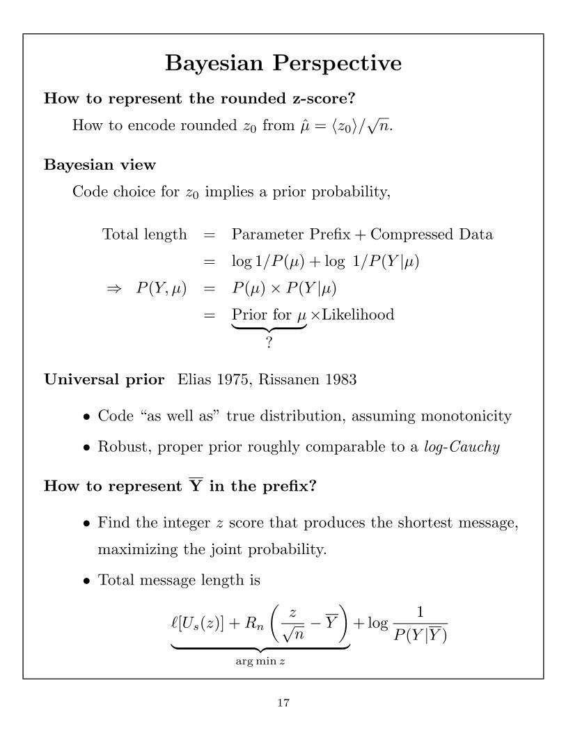
How to represent the rounded z-score?

How to encode rounded z0 from µ̂ = 〈z0〉/√n.

Bayesian view

Code choice for z0 implies a prior probability,

Total length = Parameter Prefix + Compressed Data

= log 1/P (µ) + log 1/P (Y |µ)

⇒ P (Y, µ) = P (µ)× P (Y |µ)

= Prior for µ︸ ︷︷ ︸?

×Likelihood

Universal prior Elias 1975, Rissanen 1983

• Code “as well as” true distribution, assuming monotonicity

• Robust, proper prior roughly comparable to a log-Cauchy

How to represent Y in the prefix?

• Find the integer z score that produces the shortest message,

maximizing the joint probability.

• Total message length is

`[Us(z)] +Rn

(z√n− Y

)︸ ︷︷ ︸

arg min z

+ log1

P (Y |Y )

17

Universal Priors

Simple example

Interleave continuation bits with binary form,

5 = 1012 ⇒ 11 01 10

Length is roughly 2 log z, implying p(z) ≈ 1/z2, or Cauchy-like

tails.

Recursive log

Send a sequence of blocks,each giving length of next. Define

log∗ x = log x+ log log x+ log log log x+ · · ·

where sum includes only positive terms. Series is summable,

∞∑j=1

2− log∗ j ≈ 2.8 = 21.5 <∞

Probabilities

Define p∗(0) = 1/2 and for j = 1, 2, 3, . . . ,

p∗(j) = 2−(log∗ j+2.5) = c×(

1j

)× 1

log j× 1

log log j× · · ·

Very, very thick tails

log∗(x) ≈ log x+ 2 log log x⇒ log Cauchy

18

Universal Codes

j Cauchy U(j) `[U(j)]

0 0 0 1 bit

1 10 100 3

2 1100 1010 4

3 1110 10110 5

4 110100 101110 6

5 110110 1011110 7

6 111100 1011111 7

· · ·

100 14 bits 14 bits

1000 20 19

10000 28 23

• Length of Cauchy code is 2 log j

• Length `[U(x)] = c+ log 〈x〉+ log log 〈x〉+ log log log 〈x〉+ · · ·,with rounding embedded, U(x) = U(〈x〉).

• Signed universal appends sign bit, Us(j) = U(j) ‖ (+/−)

19

Optimal Parameter Code

Optimal estimate

µ̂ = z/√n, arg min

z`[Us(z)] +Rn(z/

√n− Y )

Table on SE grid

Y z = 0 1 2 3 4

0 1.0 4.7 7.9 12.5 18.5

1/√n 1.7 4.0 5.7 8.9 13.5

2/√n 3.9 4.7 5.0 6.7 9.9

3/√n 7.5 6.9 5.7 6.0 7.7

4/√n 12.5 10.5 7.9 6.7 7.0

Note

• Code a non-zero parameter once |z| > 2.4.

• Decision rule resembles familiar normal test.

• Shrinkage stops once |z| =√n Y > 5.

Reference

“Local asymptotics and the minimum description length”

http:www-stat.wharton.upenn.edu/∼bob

20

Graph of Codebook

Vertical Axis: Bits are the excess `[Us(zµ)] +Rn(Y − µ̂) over

minimum determined by the log likelihood at Y .

Horizontal Axis: z =√nY , the usual z-score.

21

Alternative Asymptotic Analysis

Asymptotic code length Rissanen’s MDL (1983)

Asymptotic analysis of optimal code length, with n→∞ and

µ = E Y fixed so that z =√nY is large:

Code length = `[Us(√nY )] + log

1P (Y |Y )

+ c

≈ log√nY + log

1P (Y |Y )

= 12 logn+ log

1P (Y |Y )

+Op(1)

Implication for prefix length

To code any mean value requires 12 logn bits.

Model selection

Use a special one-bit code for zero. Code any non-zero

parameter using 1 + 12 logn bits:

Parameter Prefix

0 0

z 6= 0 1 ‖ 12 logn bits for z

Penalized likelihood BIC

Reject H0 : µ = 0 and code a non-zero mean only if

logP (Y |Y )− logP (Y |µ = 0) > 12 logn or |z| >

√logn.

22

Spike and Slab Prior

Code = Probability

Recall that the choice of coding method implies a probability

model. This applies to the parameter codes as well.

⇒ Very Bayesian point of view.

Implicit assumption

If we knew that |µ| < 12 , then to grid this interval to precision

1/√n requires log

√n = 1

2 logn bits. The larger the range

allowed for µ, the larger the number of bits.

Associated prior on µ

• If we do not code a mean, then we represent µ = 0 with just

1 bit, implying a probability of 1/2.

• If we do code a mean, then we represent µ using 1 + 1/2 logn

bits, corresponding to a uniform distribution on |µ| < 12 .

Natural prior?

Parameter is either exactly zero, or anywhere in allowed range.

Asymptotics essentially force large z score for any µ 6= 0.

Impact of prior

Priors are much more important in model selection than

elsewhere.

23

Graph of BIC Codebook

Vertical Axis: Bits are the excess 12 logn+Rn(Y − µ̂) over

minimum determined by the log likelihood at Y , with n = 1024 and

−16 < µ ≤ 16

Horizontal Axis: z =√nY , the usual z-score.

24

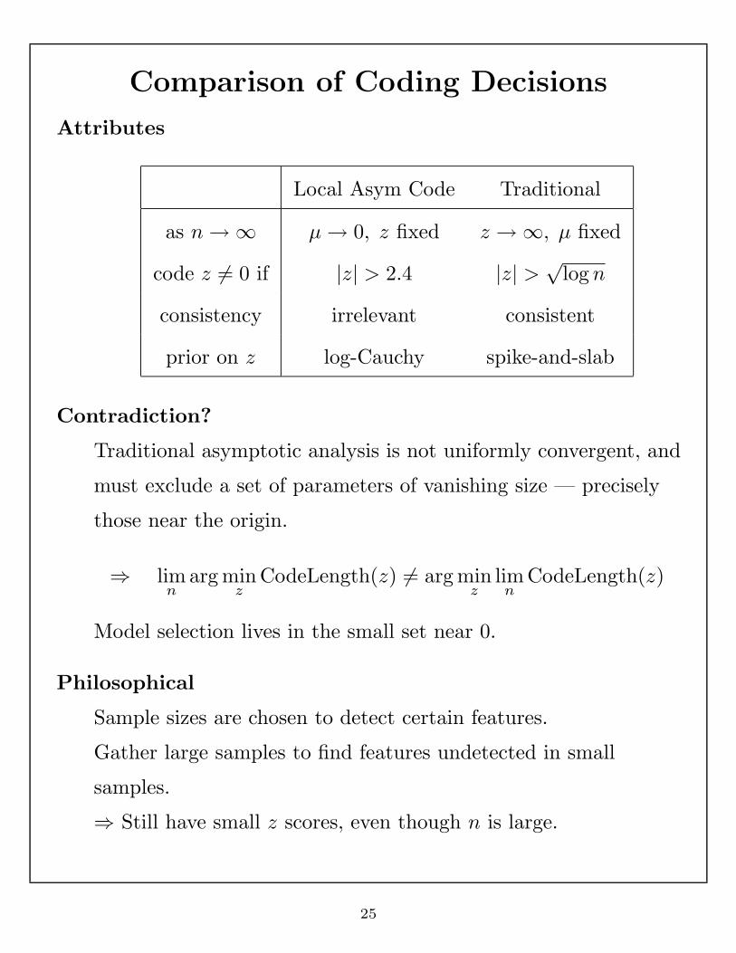
Comparison of Coding Decisions

Attributes

Local Asym Code Traditional

as n→∞ µ→ 0, z fixed z →∞, µ fixed

code z 6= 0 if |z| > 2.4 |z| >√

logn

consistency irrelevant consistent

prior on z log-Cauchy spike-and-slab

Contradiction?

Traditional asymptotic analysis is not uniformly convergent, and

must exclude a set of parameters of vanishing size — precisely

those near the origin.

⇒ limn

arg minz

CodeLength(z) 6= arg minz

limn

CodeLength(z)

Model selection lives in the small set near 0.

Philosophical

Sample sizes are chosen to detect certain features.

Gather large samples to find features undetected in small

samples.

⇒ Still have small z scores, even though n is large.

25

Review and Next Steps

So far

Information theory provides another view of modeling: good

models produce short codes.

Parameter coding

Method of coding rounded parameter corresponds to a prior on

the parameter space, with coding making the prior very explicit.

Different codes/priors lead to different modeling criteria:

• Local asymptotics suggest fixed threshold near 2.4.

• Large z arguments lead to BIC with a threshold√

logn.

Regression

Same coding ideas, but now with multiple parameters.

Again, choose the model producing the shortest message

(parameters + data).

Additional feature in regression

Codes for regression must also identify the chosen predictors as

well as give the values of any parameter estimates.

26