inis.jinr.ruinis.jinr.ru/sl/m_mathematics/mref_references/mason, hanscomb... · chapter 9 solution...

Chapter 9

Solution of Integral Equations

9.1 Introduction

In this chapter we shall discuss the application of Chebyshev polynomial tech-niques to the solution of Fredholm (linear) integral equations, which are clas-sified into three kinds taking the following generic forms:

First kind: Given functions K(x, y) and g(x), find a function f(y) on [a, b]such that for all x ∈ [a, b]

∫ b

a

K(x, y)f(y) dy = g(x); (9.1)

Second kind: Given functions K(x, y) and g(x), and a constant λ not pro-viding a solution of (9.3) below, find a function f(y) on [a, b] such thatfor all x ∈ [a, b]

f(x) − λ∫ b

a

K(x, y)f(y) dy = g(x); (9.2)

Third kind: Given a function K(x, y), find values (eigenvalues) of the con-stant λ for which there exists a function (eigenfunction) f(y), not van-ishing identically on [a, b], such that for all x ∈ [a, b]

f(x) − λ∫ b

a

K(x, y)f(y) dy = 0. (9.3)

Equations of these three kinds may be written in more abstract terms asthe functional equations

Kf = g, (9.4)

f − λKf = g, (9.5)

f − λKf = 0, (9.6)

where K represents a linear mapping (here an integral transformation) fromsome function space F into itself or possibly (for an equation of the first kind)into another function space G, g represents a given element of F or G asappropriate and f is an element of F to be found.

A detailed account of the theory of integral equations is beyond the scopeof this book — we refer the reader to Tricomi (1957), for instance. However,

© 2003 by CRC Press LLC

it is broadly true (for most of the kernel functions K(x, y) that one is likely tomeet) that equations of the second and third kinds have well-defined and well-behaved solutions. Equations of the first kind are quite another matter—herethe problem will very often be ill-posed mathematically in the sense of eitherhaving no solution, having infinitely many solutions, or having a solution fthat is infinitely sensitive to variations in the function g. It is essential thatone reformulates such a problem as a well-posed one by some means, beforeattempting a numerical solution.

In passing, we should also mention integral equations of Volterra type,which are similar in form to Fredholm equations but with the additional prop-erty that K(x, y) = 0 for y > x, so that∫ b

a

K(x, y)f(y) dy

is effectively ∫ x

a

K(x, y)f(y) dy.

A Volterra equation of the first kind may often be transformed into one of thesecond kind by differentiation. Thus∫ x

a

K(x, y)f(y) dy = g(x)

becomes, on differentiating with respect to x,

K(x, x)f(x) +∫ x

a

∂

∂xK(x, y)f(y) dy =

ddxg(x).

It is therefore unlikely to suffer from the ill-posedness shown by general Fred-holm equations of the first kind. We do not propose to discuss the solution ofVolterra equations any further here.

9.2 Fredholm equations of the second kind

In a very early paper, Elliott (1961) studied the use of Chebyshev polynomialsfor solving non-singular equations of the second kind

f(x) − λ∫ b

a

K(x, y)f(y) dy = g(x), a ≤ x ≤ b, (9.7)

and this work was later updated by him (Elliott 1979). Here K(x, y) isbounded in a ≤ x, y ≤ b, and we suppose that λ is not an eigenvalue of(9.3). (If λ were such an eigenvalue, corresponding to the eigenfunction φ(y),then any solution f(y) of (9.7) would give rise to a multiplicity of solutions ofthe form f(y) + αφ(y) where α is an arbitrary constant.)


For simplicity, suppose that a = −1 and b = 1. Assume that f(x) may beapproximated by a finite sum of the form

N∑′′

j=0

ajTj(x). (9.8)

Then we can substitute (9.8) into (9.7) so that the latter becomes the approx-imate equation

N∑′′

j=0

ajTj(x) − λN∑′′

j=0

aj

∫ 1

−1

K(x, y)Tj(y) dy ∼ g(x), −1 ≤ x ≤ 1. (9.9)

We need to choose the coefficients aj so that (9.9) is satisfied as well aspossible over the interval −1 ≤ x ≤ 1. A reasonably good way of achievingthis is by collocation — requiring equation (9.9) to be an exact equality atthe N + 1 points (the extrema of TN(x) on the interval)

x = yi,N = cosiπ

N,

so thatN∑′′

j=0

aj(Pij − λQij) = g(yi,N ), i = 0, . . . , N, (9.10)

where

Pij = Tj(yi,N ), Qij =∫ 1

−1

K(yi,N , y)Tj(y) dy. (9.11)

We thus have N + 1 linear equations to solve for the N + 1 unknowns aj .

As an alternative to collocation, we may choose the coefficients bi,k so thatKM (yi,N , y) gives a least squares or minimax approximation to K(yi,N , y).

If we cannot evaluate the integrals in (9.11) exactly, we may do so approx-imately, for instance, by replacing each K(yi,N , y) with a polynomial

KM (yi,N , y) =M∑′′

k=0

bi,kTk(y) (9.12)

for some1 M > 0, with Chebyshev coefficients given by

bi,k =2M

M∑′′

m=0

K(yi,N , ym,M )Tk(ym,M ), k = 0, . . . ,M, (9.13)

1There does not need to be any connection between the values of M and N .


whereym,M = cos

mπ

M, m = 0, . . . ,M.

As in the latter part of Section 6.3.2, we can then show that

KM (yi,N , ym,M ) = K(yi,N , ym,M ), m = 0, . . . ,M,

so that, for each i, KM (yi,N , y) is the polynomial of degree M in y, interpo-lating K(yi,N , y) at the points ym,M .

From (2.43) it is easily shown that

∫ 1

−1

Tn(x) dx =

{ −2n2 − 1

, n even,

0, n odd.(9.14)

Hence

Qij ≈∫ 1

−1

KM (yi,N , y)Tj(y) dy

=M∑′′

k=0

bi,k

∫ 1

−1

Tk(y)Tj(y) dy

= 12

M∑′′

k=0

bi,k

∫ 1

−1

{Tj+k(y) + T|j−k|(y)} dy

= −M∑′′

k=0j±k even

bi,k

{1

(j + k)2 − 1+

1(j − k)2 − 1

}

= −2M∑′′

k=0j±k even

bi,kj2 + k2 − 1

(j2 + k2 − 1)2 − 4j2k2, (9.15)

giving us the approximate integrals we need.

Another interesting approach, based on ‘alternating polynomials’ (whoseequal extrema occur among the given data points), is given by Brutman(1993). It leads to a solution in the form of a sum of Chebyshev polyno-mials, with error estimates.

9.3 Fredholm equations of the third kind

We can attack integral equations of the third kind in exactly the same way asequations of the second kind, with the difference that we have g(x) = 0.


Thus the linear equations (9.10) become

N∑′′

j=0

aj(Pij − λQij) = 0, i = 0, . . . , N. (9.16)

Multiplying each equation by T�(yi,N ) and carrying out a∑′′ summation

over i (halving the first and last terms), we obtain (after approximating K byKM ) the equations

MN

4a� = λ

N∑′′

j=0

aj ×

× M∑′′

k=0

N∑′′

i=0

M∑′′

m=0

T�(yi,N )K(yi,N , ym,M )Tk(ym,M )∫ 1

−1

Tk(y)Tj(y) dy

,

(9.17)

which is of the formMN

4a� = λ

N∑j=0

ajA�j (9.18)

or, written in terms of vectors and matrices,

MN

4a = λAa. (9.19)

Once the elements of the (N+1)×(N+1) matrix A have been calculated, thisis a straightforward (unsymmetric) matrix eigenvalue problem, which maybe solved by standard techniques to give approximations to the dominanteigenvalues of the integral equation.

9.4 Fredholm equations of the first kind

Consider now a Fredholm integral equation of the first kind, of the form

g(x) =∫ b

a

K(x, y)f(y) dy, c ≤ x ≤ d. (9.20)

We can describe the function g(x) as an integral transform of the functionf(y), and we are effectively trying to solve the ‘inverse problem’ of determiningf(y) given g(x).

For certain special kernels K(x, y), a great deal is known. In particular,the choices

K(x, y) = cosxy, K(x, y) = sinxy and K(x, y) = e−xy,


with [a, b] = [0,∞), correspond respectively to the well-known Fourier cosinetransform, Fourier sine transform and Laplace transform. We shall not pursuethese topics specifically here, but refer the reader to the relevant literature(Erdelyi et al. 1954, for example).

Smooth kernels in general will often lead to inverse problems that areill-posed in one way or another.

For example, if K is continuous and f is integrable, then it can be shownthat g = Kf must be continuous — consequently, if we are given a g that isnot continuous then no (integrable) solution f of (9.20) exists.

Uniqueness is another important question to be considered. For exampleGroetsch (1984) notes that the equation∫ π

0

x sin y f(y) dy = x

has a solutionf(y) = 1

2 .

However, it has an infinity of further solutions, including

f(y) = 12 + sinny (n = 2, 3, . . .).

An example of a third kind of ill-posedness, given by Bennell (1996), isbased on the fact that, if K is absolutely integrable in y for each x, then bythe Riemann–Lebesgue theorem,

φn(x) ≡∫ b

a

K(x, y) cosny dy → 0 as n→ ∞.

Hence∫ b

a

K(x, y)(f(y) + α cosny) dy = g(x) + αφn(x) → g(x) as n→ ∞,

where α is an arbitrary positive constant. Thus a small perturbation

δg(x) = αφn(x)

in g(x), converging to a zero limit as n→ ∞, can lead to a perturbation

δf(y) = α cosny

in f(y) which remains of finite magnitude α for all n. This means that thesolution f(y) does not depend continuously on the data g(x), and so theproblem is ill-posed.

We thus see that it is not in fact necessarily advantageous for the func-tion K to be smooth. Nevertheless, there are ways of obtaining acceptablenumerical solutions to problems such as (9.20). They are based on the tech-nique of regularisation, which effectively forces an approximate solution to beappropriately smooth. We return to this topic in Section 9.6 below.


9.5 Singular kernels

A particularly important class of kernels, especially in the context of the studyof Chebyshev polynomials in integral equations, comprises the Hilbert kernel

K(x, y) =1

x− y (9.21)

and other related ‘Hilbert-type’ kernels that behave locally like (9.21) in theneighbourhood of x = y.

9.5.1 Hilbert-type kernels and related kernels

If [a, b] = [−1, 1] and

K(x, y) =w(y)y − x,

where w(y) is one of the weight functions (1 + y)α(1 − y)β with α, β = ± 12 ,

then there are direct links of the form (9.20) between Chebyshev polynomialsof the four kinds (Fromme & Golberg 1981, Mason 1993).

Theorem 9.1

πUn−1(x) =∫ 1

−1

K1(x, y)Tn(y) dy, (9.22a)

−πTn(x) =∫ 1

−1

K2(x, y)Un−1(y) dy, (9.22b)

πWn(x) =∫ 1

−1

K3(x, y)Vn(y) dy, (9.22c)

−πVn(x) =∫ 1

−1

K4(x, y)Wn(y) dy (9.22d)

where

K1(x, y) =1√

1 − y2 (y − x),

K2(x, y) =

√1 − y2

(y − x),

K3(x, y) =√

1 + y√1 − y (y − x)

,

K4(x, y) =√

1 − y√1 + y (y − x)

,

and each integral is to be interpreted as a Cauchy principal value integral.


Proof: In fact, formulae (9.22a) and (9.22b) correspond under the transformationx = cos θ to the trigonometric formulae∫ π

0

cosnφ

cosφ − cos θdφ = π

sinnθ

sin θ, (9.23)

∫ π

0

sinnφ sinφ

cosφ − cos θdφ = −π cosnθ, (9.24)

which have already been proved in another chapter (Lemma 8.3). Formulae (9.22c)

and (9.22d) follow similarly from Lemma 8.5. ••From Theorem 9.1 we may immediately deduce integral relationships be-

tween Chebyshev series expansions of functions as follows.

Corollary 9.1A

1. If f(y) ∼ ∑∞n=1 anTn(y) and g(x) ∼ π

∑∞n=1 anUn−1(x) then

g(x) =∫ 1

−1

f(y)√1 − y2 (y − x)

dy. (9.25a)

2. If f(y) ∼ ∑∞n=1 bnUn−1(y) and g(x) ∼ π

∑∞n=1 bnTn(x) then

g(x) = −∫ 1

−1

√1 − y2 f(y)(y − x)

dy. (9.25b)

3. If f(y) ∼ ∑∞n=1 cnVn(y) and g(x) ∼ π

∑∞n=1 cnWn(x) then

g(x) =∫ 1

−1

√1 + y f(y)√

1 − y (y − x)dy. (9.25c)

4. If f(y) ∼ ∑∞n=1 dnWn(y) and g(x) ∼ π

∑∞n=1 dnVn(x) then

g(x) = −∫ 1

−1

√1 − y f(y)√

1 + y (y − x)dy. (9.25d)

Note that these expressions do not necessarily provide general solutions tothe integral equations (9.25a)–(9.25d), but they simply show that the relevantformal expansions are integral transforms of each other.

These relationships are useful in attacking certain engineering problems.Gladwell & England (1977) use (9.25a) and (9.25b) in elasticity analysis andFromme & Golberg (1979) use (9.25c), (9.25d) and related properties of Vn

and Wn in analysis of the flow of air near the tip of an airfoil.

To proceed to other kernels, we note that by integrating equations (9.22a)–(9.22d) with respect to x, after premultiplying by the appropriate weights, wecan deduce the following eigenfunction properties of Chebyshev polynomialsfor logarithmic kernels. The details are left to the reader (Problem 4).


Theorem 9.2 The integral equation

λφ(x) =∫ 1

−1

1√1 − y2

φ(y)K(x, y) dy (9.26)

has the following eigensolutions and eigenvalues λ for the following kernelsK.

1. K(x, y) = K5(x, y) = log |y − x|;φ(x) = φn(x) = Tn(x), λ = λn = π/n.

2. K(x, y) = K6(x, y) = log |y − x| − log∣∣∣1 − xy − √

(1 − x2)(1 − y2)∣∣∣;

φ(x) = φn(x) =√

1 − x2 Un−1(x), λ = λn = π/n.

3. K(x, y) = K7(x, y) = log |y − x| − log∣∣2 + x+ y − 2

√1 + x

√1 + y

∣∣;φ = φn(x) =

√1 + xVn(x), λ = λn = π/(n+ 1

2 ).

4. K(x, y) = K8(x, y) = log |y − x| − log∣∣2 − x− y − 2

√1 − x√1 − y∣∣;

φ = φn(x) =√

1 − xWn(x), λ = λn = π/(n+ 12 ).

Note that each of these four kernels has a (weak) logarithmic singularityat x = y. In addition, K6 has logarithmic singularities at x = y = ±1, K7 atx = y = −1 and K8 at x = y = +1.

From Theorem 9.2 we may immediately deduce relationships between for-mal Chebyshev series of the four kinds as follows.

Corollary 9.2A With the notations of Theorem 9.2, in each of the four casesconsidered, if

f(y) ∼∞∑

k=1

akφk(y) and g(x) ∼∞∑

k=1

λkakφk(x)

then

g(x) =∫ 1

−1

1√1 − y2

K(x, y)f(y) dy.

Thus again four kinds of Chebyshev series may in principle be used to solve(9.26) for K = K5, K6, K7, K8, respectively.

The most useful results in Theorem 9.2 and its corollary are those relatingto polynomials of the first kind, where we find from Theorem 9.2 that

−πnTn(x) =

∫ 1

−1

1√1 − y2

Tn(y) log |y − x| dy (9.27)


and from Corollary 9.2A that, if

f(y) ∼∞∑

k=1

akTk(y) and g(x) ∼∞∑

k=1

−πkakTk(x), (9.28)

then

g(x) =∫ 1

−1

1√1 − y2

log |y − x| f(y) dy. (9.29)

Equation (9.29) is usually referred to as Symm’s integral equation, andclearly a Chebyshev series method is potentially very useful for such problems.We shall discuss this specific problem further in Section 9.5.2.

By differentiating rather than integrating in (9.22a), (9.22b), (9.22c) and(9.22d), we may obtain the further results quoted in Problem 5. The secondof these yields the simple equation

−nπUn−1(x) =∫ 1

−1

√1 − y2

(y − x)2Un−1(y) dy. (9.30)

This integral equation, which has a stronger singularity than (9.22a)–(9.22d),is commonly referred to as a hypersingular equation, in which the integralhas to be evaluated as a Hadamard finite-part integral (Martin 1991, forexample). A rather more general hypersingular integral equation is solved bya Chebyshev method, based on (9.30), in Section 9.7.1 below.

The ability of a Chebyshev series of the first or second kind to handleboth Cauchy principal value and hypersingular integral transforms leads usto consider an integral equation that involves both. This can be success-fully attacked, and Mason & Venturino (2002) give full details of a Galerkinmethod, together with both L2 and L∞ error bounds, and convergence proofs.

9.5.2 Symm’s integral equation

Consider the integral equation (Symm 1966)

G(x) = VF (x) =1π

∫ b

a

log |y − x|F (y) dy, x ∈ [a, b], (9.31)

which is of importance in potential theory.

This equation has a unique solution F (y) (Jorgens 1970) with endpointsingularities of the form (y− a)−

12 (b− y)−

12 . In the case a = −1, b = +1, the

required singularity is (1 − y2)−12 , and so we may write

F (y) = (1 − y2)−12 f(y), G(x) = −π−1g(x),


whereupon (9.31) becomes

g(x) = V∗f(x) =∫ 1

−1

log |y − x|√1 − y2

f(y) dy (9.32)

which is exactly the form (9.29) obtained from Corollary 9.2A.

We noted then (9.29) that if

f(y) ∼∞∑

k=1

akTk(y)

then

g(x) ∼∞∑

k=1

−πkakTk(x)

(and vice versa).

Sloan & Stephan (1992), adopt such an idea and furthermore note that

V∗T0(x) = −π log 2,

so that

f(y) ∼∞∑′

k=0

akTk(y)

if

g(x) ∼ − 12a0π log 2 −

∞∑k=1

π

kakTk(x).

Their method of approximate solution is to write

f∗(y) =n−1∑′

k=0

a∗kTk(y) (9.33)

and to require thatV∗f∗(x) = g(x)

holds at the zeros x = xi of Tn(x). Then

g(xi) = − 12a

∗0π log 2 −

n−1∑k=1

π

ka∗kTk(xi), i = 0, . . . , n− 1. (9.34)

Using the discrete orthogonality formulae (4.42), we deduce that

a∗0 = − 2nπ log 2

n−1∑i=0

g(xi), (9.35)

a∗k = − 2knπ

n−1∑i=0

g(xi)Tk(xi) (k > 0). (9.36)


Thus values of the coefficients {a∗k} are determined explicitly.

The convergence properties of the approximation f∗ to f have been estab-lished by Sloan & Stephan (1992).

9.6 Regularisation of integral equations

Consider again an integral equation of the first kind, of the form

g(x) =∫ b

a

K(x, y)f(y) dy, c ≤ x ≤ d, (9.37)

i.e. g = Kf , where K : F → G and where the given g(x) may be affected bynoise (Bennell & Mason 1989). Such a problem is said to be well posed if:

• for each g ∈ G there exists a solution f ∈ F ;

• this solution f is always unique in F ;

• f depends continuously on g (i.e., the inverse of K is continuous).

Unfortunately it is relatively common for an equation of the form (9.37) tobe ill posed, so that a method of solution is needed which ensures not only thata computed f is close to being a solution but also that f is an appropriatelysmooth function. The standard approach is called a regularisation method ;Tikhonov (1963b, 1963a) proposed an L2 approximation which minimises

I[f∗] :=∫ b

a

[Kf∗(x) − g(x)]2 dx+ λ

∫ b

a

[p(x)f∗(x)2 + q(x)f∗′(x)2] dx (9.38)

where p and q are specified positive weight functions and λ a positive ‘smooth-ing’ parameter. The value of λ controls the trade-off between the smoothnessof f∗ and the fidelity to the data g.

9.6.1 Discrete data with second derivative regularisation

We shall first make two changes to (9.38) on the practical assumptions that weseek a visually smooth (i.e., twice continuously differentiable) solution, andthat the data are discrete. We therefore assume that g(x) is known only at nordinates xi and then only subject to white noise contamination ε(xi);

g∗(xi) =∫ b

a

K(xi, y)f(y) dy + ε(xi) (9.39)

where each ε(xi) ∼ N(0, σ2) is drawn from a normal distribution with zeromean and (unknown) variance σ2. We then approximate f by the f∗λ ∈ L2[a, b]


that minimises

I[f∗] ≡ 1n

n∑i=1

[Kf∗(xi) − g∗(xi)]2 + λ

∫ b

a

[f∗′′(y)

]2dy, (9.40)

thus replacing the first integral in (9.38) by a discrete sum and the second byone involving the second derivative of f∗.

Ideally, a value λopt of λ should be chosen (in an outer cycle of iteration)to minimise the true mean-square error

R(λ) ≡ 1n

n∑i=1

[Kf∗λ(xi) − g(xi)]2 . (9.41)

This is not directly possible, since the values g(xi) are unknown. However,Wahba (1977) has shown that a good approximation to λopt may be obtainedby choosing the ‘generalised cross-validation’ (GCV) estimate λ∗opt that min-imises

V (λ) =1n ‖(I−A(λ)g‖2[

1n trace(I−A(λ))

]2 , (9.42)

whereKf∗λ = A(λ)g, (9.43)

i.e., A(λ) is the matrix which takes the vector of values g(xi) into Kf∗λ(xi).

An approximate representation is required for f∗λ . Bennell & Mason (1989)adopt a basis of polynomials orthogonal on [a, b], and more specifically theChebyshev polynomial sum

f∗λ(y) =m∑

j=0

ajTj(y) (9.44)

when [a, b] = [−1, 1].

9.6.2 Details of a smoothing algorithm (second derivative regular-isation)

Adopting the representation (9.44), the smoothing term in (9.40) is

∫ 1

−1

[f∗λ

′′(y)]2

dy = aTBa (9.45)

where a = (a2, a3, . . . , am)T and B is a matrix with elements

Bij =∫ 1

−1

P ′′i (y)P ′′

j (y) dy (i, j = 2, . . . ,m). (9.46)


The matrix B is symmetric and positive definite, with a Cholesky decompo-sition B = LLT , giving

∫ 1

−1

[f∗λ

′′(y)]2

dy =∥∥LT a

∥∥2.

Then, from (9.40),

I[f∗λ ] =1n‖Ma− g∗‖2 + λ

∥∥LT a∥∥2

(9.47)

where Mij =∫ 1

−1K(xi, y)Tj(y) dy and a = (a1, a2, . . . , am)T .

Bennell & Mason (1989) show that a0 and a1 may be eliminated by con-sidering the QU decomposition of M,

M = QU = Q[V0

], (9.48)

where Q is orthogonal, V is upper triangular of order m+ 1 and then

U =[R1 R2

0 R3

](9.49)

where R1 is a 2 × 2 matrix.

Defining a = (a0, a1)T ,

‖Ma− g∗‖2 = ‖QUa− g∗‖2

=∥∥QT (QUa− g∗)

∥∥2

= ‖Ua − e‖2 , where e = QTg∗,

= ‖R1a + R2a− e‖2 + ‖R3a− e‖2 . (9.50)

Setting a = R−11 (e−R2a),

I[f∗λ] =1n‖R3a− e‖2 + λ

∥∥LT a∥∥2. (9.51)

The problem of minimising I over a now involves only the independentvariables a2, . . . , am, and requires us to solve the equation

(HTH + nλI)b = HT e (9.52)

where b = LT a and H = R3(LT )−1.

Henceb = (HTH + nλI)−1HT e (9.53)


and it can readily be seen that the GCV matrix is

A(λ) = H(HTH + nλI)−1HT . (9.54)

The algorithm thus consists of solving the linear system (9.52) for a givenλ while minimising V (λ) given by (9.42).

Formula (9.42) may be greatly simplified by first determining the singularvalue decomposition (SVD) of H

H = WΛXT (W, X orthogonal)

where

Λ =[∆0

](∆ = diag(di)).

Then

V (λ) =∑m−1

k=1 [nλ(d2k + nλ)−1]2z2

k +∑m−2

k=1 z2k∑m−1

k=1 λ(d2k + nλ)−1 + (n−m− 1)n−1

(9.55)

where z = WT e.

The method has been successfully tested by Bennell & Mason (1989) on anumber of problems of the form (9.37), using Chebyshev polynomials. It wasnoted that there was an optimal choice of the numberm of basis functions, be-yond which the approximation f∗λ deteriorated on account of ill-conditioning.In Figures 9.1–9.3, we compare the true solution (dashed curve) with thecomputed Chebyshev polynomial solution (9.44) (continuous curve) for thefunction f(y) = e−y and equation∫ ∞

0

e−xy f(y) dy =1

1 + x, 0 < x <∞,

with

• ε(x) ∼ N(0, .0052) and m = 5,

• ε(x) ∼ N(0, .012) and m = 5,

• ε(x) ∼ N(0, .012) and m = 10.

No significant improvement was obtained for any other value of m.

9.6.3 A smoothing algorithm with weighted function regularisa-tion

Some simplifications occur in the above algebra if, as proposed by Mason &Venturino (1997), in place of (9.40) we minimise the functional

I[f∗] ≡ 1n

n∑i=1

[Kf∗(xi) − g(xi)]2 + λ

∫ b

a

w(y)[f∗(y)]2 dy. (9.56)


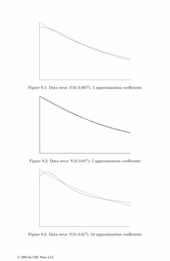
Figure 9.1: Data error N(0, 0.0052); 5 approximation coefficients




This is closer to the Tikhonov form (9.38) than is (9.40), and involves weakerassumptions about the smoothness of f .

Again we adopt an orthogonal polynomial sum to represent f∗. We choosew(x) to be the weight function corresponding to the orthogonality. In par-ticular, for the first-kind Chebyshev polynomial basis on [−1, 1], and the ap-proximation

f∗λ(y) =m∑

j=0

ajTj(y), (9.57)

the weight function is of course w(x) = 1/√

1 − x2.

The main changes to the procedure of Section 9.6.2 are that

• in the case of (9.56) we do not now need to separate a0 and a1 off fromthe other coefficients ar, and

• the smoothing matrix corresponding to B in (9.46) becomes diagonal,so that no LLT decomposition is required.

For simplicity, we take the orthonormal basis on [−1, 1], replacing (9.57) with

f∗λ(y) =m∑

j=0

ajφj(y) =m∑

j=0

aj [Tj(y)/nj] , (9.58)

where

n2j =

{2/π, j > 0;1/π, j = 0. (9.59)

Define two inner products (respectively discrete and continuous);

〈u , v〉d =n∑

k=1

u(xk)v(xk); (9.60)

〈u , v〉c =∫ 1

−1

w(x)u(x)v(x) dx. (9.61)

Then the minimisation of (9.56), for f∗ given by (9.58), leads to the systemof equations

m∑j=0

aj 〈Kφi , Kφj〉d − 〈Kφi , g∗〉d + nλm∑

j=0

aj 〈φi , φj〉c = 0, i = 0, . . . ,m.

(9.62)Hence

(QTQ + nλI)a = QTg∗ (9.63)


(as a consequence of the orthonormality), where

Qk,j = (Kφj)(xk) (9.64)

and a, g∗ are vectors with components aj and g∗(xj), respectively.

To determine f∗ we need to solve (9.63) for aj , with λ minimising V (λ)as defined in (9.42). The matrix A(λ) in (9.42) is to be such that

Kf∗ = A(λ)g∗. (9.65)

Now Kf∗ ={∑

j ajKφj(xk)}

= Qa and hence, from (9.63)

A(λ) = Q(QTQ + nλI)−1QT . (9.66)

9.6.4 Evaluation of V (λ)

It remains to clarify the remaining details of the algorithm of Section 9.6.3,and in particular to give an explicit formula for V (λ) based on (9.66).

LetQ = WΛXT (9.67)

be the singular value decomposition of Q, where W is n×n orthogonal, X is(m+ 1) × (m+ 1) orthogonal and

Λ =[∆m

0

]n×(m+1)

. (9.68)

Definez = [zk] = WTg. (9.69)

From (9.68),ΛTΛ = diag(d2

0, . . . , d2m). (9.70)

It follows thatA(λ) = WB(λ)WT (9.71)

whereB(λ) = Λ(ΛTΛ + nλI)−1ΛT (9.72)

so that B(λ) is the n× n diagonal matrix with elements

Bkk =d2

k

d2k + nλ

(0 ≤ k ≤ m); Bkk = 0 (k > m). (9.73)


From (9.71) and (9.72)

‖(I−A(λ))g‖2 = ‖(I−A(λ))Wz‖2

=∥∥WT (I−A(λ))Wz

∥∥2

=∥∥(I−WTA(λ)W)z

∥∥2

= ‖(I−B(λ))z‖2

=m∑

i=0

(nλ

d2i + nλ

)2

z2i +

n−1∑i=m+1

z2i .

Thus

‖(I−A(λ))g‖2 =m∑

i=0

n2e2i z2i +

n∑i=m+1

z2i (9.74)

whereei(λ) =

λ

d2i + nλ

. (9.75)

Also

trace(I−A(λ)) = traceWT (I−A(λ))W

= trace(I−B(λ))

=m∑

i=0

nλ

d2i + nλ

+n−1∑

i=m+1

1.

Thus

trace(I−A(λ)) =m∑

i=0

n2e2i + (n−m− 1). (9.76)

Finally, from (9.75) and (9.76), together with (9.42), it follows that

V (λ) =

m∑0

ne2i z2i +

1n

n∑m+1

z2i

[m∑0

ne2i +n−m− 1

n

]2 . (9.77)

9.6.5 Other basis functions

It should be pointed out that Chebyshev polynomials are certainly not theonly basis functions that could be used in the solution of (9.37) by regulari-sation. Indeed there is a discussion by Bennell & Mason (1989, Section ii) ofthree alternative basis functions, each of which yields an efficient algorithmicprocedure, namely:


1. a kernel function basis {K(xi, y)},

2. a B-spline basis, and

3. an eigenfunction basis.

Of these, an eigenfunction basis is the most convenient (provided that eigen-functions are known), whereas a kernel function basis is rarely of practicalvalue. A B-spline basis is of general applicability and possibly comparableto, or slightly more versatile than, the Chebyshev polynomial basis. See Ro-driguez & Seatzu (1990) and also Bennell & Mason (1989) for discussion ofB-spline algorithms.

9.7 Partial differential equations and boundary integral equationmethods

Certain classes of partial differential equations, with suitable boundary con-ditions, can be transformed into integral equations on the boundary of thedomain. This is particularly true for equations related to the Laplace oper-ator. Methods based on the solution of such integral equations are referredto as boundary integral equation (BIE) methods (Jaswon & Symm 1977, forinstance) or, when they are based on discrete element approximations, asboundary element methods (BEM) (Brebbia et al. 1984). Chebyshev polyno-mials have a part to play in the solution of BIEs, since they lead typically tokernels related to the Hilbert kernel discussed in Section 9.5.1.

We now illustrate the role of Chebyshev polynomials in BIE methods for aparticular mixed boundary value problem for Laplace’s equation, which leadsto a hypersingular boundary integral equation.

9.7.1 A hypersingular integral equation derived from a mixedboundary value problem for Laplace’s equation

Derivation

In this section we tackle a ‘hard’ problem, which relates closely to the hyper-singular integral relationship (9.30) satisfied by Chebyshev polynomials of thesecond kind. The problem and method are taken from Mason & Venturino(1997).

Consider Laplace’s equation for u(x, y) in the positive quadrant

∆u = 0, x, y ≥ 0, (9.78)

subject to (see Figure 9.4)


� x

�

y

a

b

L

u = 0

u = 0

u = 0

hu+ ux = g

↗ u bounded

Figure 9.4: Location of the various boundary conditions (9.79)

u(x, 0) = 0, x ≥ 0, (9.79a)

hu(0, y) + ux(0, y) = g(y), 0 < a ≤ y ≤ b, (9.79b)

u(0, y) = 0, 0 ≤ y < a; b < y, (9.79c)

u(x, y) is bounded, x, y → ∞. (9.79d)

Thus the boundary conditions are homogeneous apart from a window L ≡[a, b] of radiation boundary conditions, and the steady-state temperature dis-tribution in the positive quadrant is sought. Here the boundary conditionsare ‘mixed’ in two senses: involving both u and ux on L and splitting into twodifferent operators on x = 0. Such problems are known to lead to Cauchy sin-gular integral equations (Venturino 1986), but in this case a different approachleads to a hypersingular integral equation closely related to (9.30).

By separation of variables in (9.78), using (9.79a) and (9.79d), we findthat

u(x, y) =∫ ∞

0

A(µ) sin(µy) exp(−µx) dµ. (9.80)

The zero conditions (9.79c) on the complement Lc of L give

u(0, y) = limx→0+

∫ ∞

0

A(µ) sin(µy) exp(−µx) dµ = 0, y ∈ Lc, (9.81)

and differentiation of (9.80) with respect to x in L gives

ux(0, y) = − limx→0+

∫ ∞

0

µA(µ) sin(µy) exp(−µx) dµ = 0, y ∈ L. (9.82)


Substitution of (9.80) and (9.82) into (9.79b) leads to

limx→0+

∫ ∞

0

(h− µ)A(µ) sin(µy) exp(−µx) dµ = g(y), y ∈ L. (9.83)

Then (9.81) and (9.83) are a pair of dual integral equations for A(µ), andfrom which we can deduce u by using (9.80).

To solve (9.81) and (9.83), we define a function B(y) as

B(y) := u(0, y) =∫ ∞

0

A(µ) sin(µy) dµ, y ≥ 0. (9.84)

Then, from (9.81)B(y) = 0, y ∈ Lc, (9.85)

and, inverting the sine transform (9.84) and using (9.85),∫L

B(t) sin(st) dt = 12πA(s). (9.86)

Substituting (9.86) in the integral equation (9.83) gives us

hB(y) − 2π

∫L

I(t) dt = g(t), y ∈ L (9.87)

where

I(t) = limx→0+

∫ ∞

0

µ sin(µt) exp(−µx) dµ

= 12 lim

x→0+

∫ ∞

0

µ [cosµ(t− y) − cosµ(t+ y)] exp(−µx) dµ. (9.88)

This simplifies (see Problem 7) to

I(t) = 12 lim

x→0+

[x2 − (t− y)2

(x2 + (t− y)2)2− x2 − (t+ y)2

(x2 + (t+ y)2)2

]

= − 12

[1

(t− y)2− 1

(t+ y)2

]. (9.89)

Substituting (9.89) into (9.87), we obtain the hypersingular integral equa-tion, with strong singularity at t = y,

hB(y) +1π

∫L

B(t)[

1(t− y)2

− 1(t+ y)2

]dt = g(y), y ∈ L, (9.90)

from which B(y) is to be determined, and hence A(s) from (9.86) and u(x, y)from (9.80).


Method of solution

Continuing to follow Mason & Venturino (1997), equation (9.90) can be rewrit-ten in operator form as

Aφ ≡ (h+ H + K)φ = f (9.91)

where H is a Hadamard finite-part integral and K is a compact perturbation,given by

(Hφ)(x) =∫ 1

−1

φ(s)(s− x)2

ds, −1 < x < 1, (9.92)

(Kφ)(x) ≡∫ 1

−1

K(x, s)φ(s) ds =∫ 1

−1

φ(s)(s+ x)2

ds, −1 < x < 1, (9.93)

andf(x) = g

(12 (b− a)x+ 1

2 (b+ a)). (9.94)

It is clear that φ(x) must vanish at the end points ±1, since it representsboundary values, and moreover it should possess a square-root singularity(Martin 1991). Hence we write

φ(x) = w(x)y(x), where w(x) =√

1 − x2. (9.95)

We note also that the Hadamard finite-part operator maps second kindChebyshev polynomials into themselves, as shown by Mason (1993) and Mar-tin (1992) and indicated in (9.30) above; in fact

H(wU�)(x) = −π(+ 1)U�(x), ≥ 0. (9.96)

Solution of (9.86) in terms of second-kind polynomials is clearly suggested,namely

y(x) =∞∑

�=0

c�U�(x), (9.97)

where the coefficients c� are to be determined, and we therefore define aweighted inner product

〈u , v〉w :=∫ 1

−1

w(t)u(t)v(t) dt

and observe that‖U�‖2

w = 12π, ≥ 0. (9.98)

We also expand both f(x), the right-hand side of (9.91), and K(x, t) insecond-kind polynomials

f(x) =∞∑

i=0

fjUj(x), where fj =2π〈f , Uj〉w , (9.99)


K(x, t) =∞∑

i=0

∞∑j=0

KijUi(x)Uj(t), (9.100)

so that (9.93), (9.97) and (9.98) give

Kφ =∞∑

i=0

∞∑j=0

∞∑�=0

c�Kij

∫ 1

−1

w(t)Ui(x)Uj(t)u�(t) dt

=∞∑

i=0

∞∑j=0

∞∑�=0

c�KijUi(x) ‖Uj‖2w δj�

= 12π

∞∑�=0

c�

∞∑i=0

Ki�Ui(x). (9.101)

Substituting (9.95), (9.97), (9.99), (9.101) and (9.99) into (9.91):

hw∞∑

�=0

c�U�(x) − π∞∑

�=0

(+ 1)c�U�(x) + 12π

∞∑�=0

c�

∞∑i=0

Ki�Ui(x) =∞∑

j=0

fjUj(x).

(9.102)

Taking the weighted inner product with Uj :

h

∞∑�=0

c� 〈wU� , Uj〉w − π∞∑

�=0

(+ 1)c� 〈U� , Uj〉w +

+ 12π

∞∑�=0

c�

∞∑i=0

Ki� 〈Ui , Uj〉w =12πfj . (9.103)

Define

bjl := 〈wU� , Uj〉w =∫ 1

−1

(1 − x2)U�(x)Uj(x) dx. (9.104)

Then it can be shown (Problem 8) that

bj� =

1(+ j + 2)2 − 1

− 1(− j)2 − 1

, j + even,

0, otherwise.(9.105)

Hence, from (9.103),

h

∞∑�=0

bj�c� − 12π

2(j + 1)cj + (12π)2

∞∑�=0

Kj�c� =12πfj , 0 ≤ j <∞. (9.106)

Reducing (9.106) to a finite system, to solve for approximate coefficients c�,we obtain

h

N−1∑�=0

bj�c�− 12π

2(j+1)cj+(12π)2

N−1∑�=0

Kj�c� =12πfj , 0 ≤ j < N−1. (9.107)


Table 9.1: Results for K = 0, φ(x) =√

1 − x2 expxN condition number ‖eN‖∞1 1.932 2.81 5 × 10−1

4 4.17 5 × 10−3

8 6.54 2 × 10−8

16 10.69 1.5 × 10−13

Example 9.1: The method is tested by Mason & Venturino (1997) for a slightly

different problem, where the well-behaved part K of the problem is set to zero and

the function f is chosen so that φ(x) ≡ √1− x2 exp x. The condition number of the

matrix of the linear system (9.107) defining cj is compared in Table 9.1 with the

maximum error ‖eN‖∞ for various values of N , and it is clear that the conditioning

is relatively good and the accuracy achieved is excellent.

Error analysis

A rigorous error analysis has been carried out by Mason & Venturino (1997),but the detail is much too extensive to quote here. However, the conclusionreached was that, if f ∈ Cp+1[−1, 1] and the integral operator K satisfiescertain inequalities, then the method is convergent and

‖eN‖∞ ≤ C.N−(p+1) (9.108)

where the constant C depends on the smoothness of K and f but not on N .

For further studies of singular integral equations involving a Cauchy kernel,see Elliott (1989) and Venturino (1992, 1993).

9.8 Problems for Chapter 9

1. Follow through all steps in detail of the proofs of Theorem 9.1 andCorollary 9.1A.

2. Using Corollary 9.1A, find a function g(x) such that

g(x) = −∫ 1

−1

√1 − y2f(y)(y − x)

dy

in the cases


(a) f(y) = 1;(b) f(y) = y6;(c) f(y) = ey;

(d) f(y) =√

1 − y2.

3. Using Corollary 9.1A, find a function g(x) such that

g(x) = −∫ 1

−1

f(y)√1 − y2(y − x)

dy

in the cases

(a) g(x) = ex;

(b) g(x) = (1 + x)12 (1 − x)−

12 ;

(c) g(x) = x5;(d) g(x) = 1.

4. Prove Theorem 9.2 in detail. For instance, the second kernel K6 in thetheorem is derived from

K6(x, y) =∫ x

−1

K2(x, y)√1 − x2

dx.

Setting x = cos 2φ, y = cos 2ψ and tanφ = t, show that K6 simplifies to

sin 2ψ∫ t

∞

dtsin2 ψ − t2 cos2 ψ

= log∣∣∣∣ sin(φ+ ψ)sin(φ− ψ)

∣∣∣∣ .Then, by setting x = 2u2 − 1, y = 2v2 − 1 and noting that

√1 − x2 =

2u√

1 − u2,√

1 − y2 = 2v√

1 − v2, show that K6(x, y) simplifies to

log |x− y| − log∣∣∣1 − xy −

√(1 − x2)(1 − y2)

∣∣∣ .5. By differentiating rather than integrating in (9.22a), (9.22b), (9.22c)

and (9.22d), and using the properties

[√

1 − x2 Un−1(x)]′ = −nTn(x)/√

1 − x2,

[Tn(x)]′ = nUn−1(x),

[√

1 − xWn(x)]′ = (n+ 12 )Vn(x)/

√1 − x,

[√

1 + xVn(x)]′ = (n+ 12 )Wn(x)/

√1 + x,

deduce that the integral equation

λφ(x) =∫ 1

−1

1√1 − y2

φ(y)K(x, y) dy

has the following eigensolutions φ and eigenvalues λ for the followingkernels K:


(a) K(x, y) = K9(x, y) =√

1 − x2

(y − x)2− x√

1 − x2(y − x);

φ = φn(x) = Tn−1(x)/√

1 − x2, λ = λn = −nπ.

(b) K(x, y) = K10(x, y) =1 − y2

(y − x)2;

φ = φn(x) = Un−1(x), λ = λn = −nπ.

(c) K(x, y) = K11(x, y) =

√(1 − x)(1 + y)

(y − x)2−

√1 + y

2√

1 − x(y − x);

φ = φn(x) = Vn(x)/√

1 − x, λ = λn = −(n+ 12 )π.

(d) K(x, y) = K12(x, y) =

√(1 + x)(1 − y)

(y − x)2+

√1 − y

2√

1 + x(y − x);

φ = φn(x) = Wn(x)/√

1 + x, λ = λn = −(n+ 12 )π.

6. (a) Describe and discuss possible amendments that you might make tothe regularisation methods of Section 9.6 in case K has any oneof the four singular forms listed in Theorem 9.1. Does the methodsimplify?

(b) Discuss whether or not it might be better, for a general K, to useone of the Chebyshev polynomials other than Tj(x) in the approx-imation (9.44).

7. Show that∫ ∞

0

µ sinµt sinµy exp(−µx) dµ =x2 − (t− y)2

(x2 + (t− y)2)2− x2 − (t+ y)2

(x2 + (t+ y)2)2.

(This completes the determination of I(t), given by (9.88), so as toderive the hypersingular equation (9.90).)

8. Show that∫ 1

−1

(1 − x2)U�(x)Uj(x) dx =1

(+ j + 2)2 − 1− 1

(− j)2 − 1

for + j even, and that the integral vanishes otherwise. (This is a steprequired in the derivation of the solution of the hypersingular equation(9.90).)


inis.jinr.ruinis.jinr.ru/sl/m_mathematics/mref_references/mason, hanscomb... · chapter 9 solution...

Documents