innovating firms and aggregate innovationweb.stanford.edu/~klenow/klette and kortum.pdf · ·...

986

[Journal of Political Economy, 2004, vol. 112, no. 5]� 2004 by The University of Chicago. All rights reserved. 0022-3808/2004/11205-0005$10.00

Innovating Firms and Aggregate Innovation

Tor Jakob KletteUniversity of Oslo and Centre for Economic Policy Research

Samuel KortumUniversity of Minnesota, Federal Reserve Bank of Minneapolis, and National Bureau of EconomicResearch

We develop a parsimonious model of innovation to confront firm-level evidence. It captures the dynamics of individual heterogeneousfirms, describes the behavior of an industry with firm entry and exit,and delivers a general equilibrium model of technological change.While unifying the theoretical analysis of firms, industries, and theaggregate economy, the model yields insights into empirical work oninnovating firms. It accounts for the persistence of firms’ R&D in-vestment, the concentration of R&D among incumbents, the link be-tween R&D and patenting, and why R&D as a fraction of revenues ispositively correlated with firm productivity but not with firm size orgrowth.

Tor Jakob Klette died in August 2003. Tor Jakob was a wonderful friend and partnerin research. It has been very difficult to make the final revisions to this paper withouthim. We thank John Dagsvik, Jonathan Eaton, Charles Jones, Boyan Jovanovic, KalleMoene, Jarle Møen, Atle Seierstad, Peter Thompson, Galina Vereshchagina, and numerousseminar participants for helpful comments. We give special thanks to the editor andreferees, whose numerous suggestions helped to clarify the paper. Klette gratefully ac-knowledges support from the Research Council of Norway and Kortum from the NationalScience Foundation. The views expressed herein are those of the authors and not nec-essarily those of the Federal Reserve Bank of Minneapolis or the Federal Reserve System.

innovating firms 987

I. Introduction

Endogenous growth theory has sketched the bare bones of an aggregatemodel of technological change.1 Firm-level studies of research and de-velopment, productivity, patenting, and firm growth could add flesh tothese bones.2 So far they have not.

Exploiting firm-level findings for this purpose raises difficult ques-tions. For instance, studies of how R&D affects productivity and pat-enting do not address why firms conduct R&D on very different scalesin the first place. What are the sources of this heterogeneity in innovativeeffort across firms, and why is it so persistent? Why do some firms prosperwhile doing little or no R&D?3 Does a firm’s productivity adequatelymeasure innovative performance given that many innovations appearin the form of new products? Is patenting a superior indicator of in-novative output?

Firm growth is yet another measure of innovative performance. Em-pirical studies of firm growth, entry, exit, and size distribution couldcomplement the literature on R&D, productivity, and patenting.4 In fact,these two lines of research have developed independently. They deservean integrated treatment.

We construct a model of innovating firms to address these issues. Themodel is rich enough to match stylized facts from firm-level studies yetsimple enough to yield analytical results both for the dynamics of in-dividual firms and for the behavior of the economy as a whole. At theroot of the model is a Poisson process for a firm’s innovations with anarrival rate a function of its current R&D and knowledge generated byits past R&D. This specification of the innovation process is consistentwith the empirical relationship between patents and R&D at the firmlevel. We derive the optimal R&D investment rule that, together withthe innovation function, delivers firm growth rates independent of size,that is, Gibrat’s law. The stochastic process for innovation leads to het-erogeneity in the size of firms. The R&D rule, together with size het-erogeneity, captures the observed persistent differences in R&D acrossfirms.5

The foundation of our approach is closely related to Penrose’s (1959)

1 The seminal papers are Romer (1990), Grossman and Helpman (1991), and Aghionand Howitt (1992).

2 Much of this literature stems from the work of Zvi Griliches and his coworkers (seeGriliches 1990, 1995).

3 Cohen and Klepper (1996) have highlighted these puzzles.4 The classic reference is Ijiri and Simon (1977), but this literature on firm growth has

recently been revived by Amaral et al. (1998) and Sutton (1998), among others.5 The work of Thompson (1996, 2001), Peretto (1999), and Klette and Griliches (2000)

has a similar motivation. Each attempts to bring realistic features of firms into an aggregatemodel of technological change. Our approach differs from these earlier contributions bybuilding in the multiproduct nature of firms. The resulting model is particularly tractable.

988 journal of political economy

theory of the “innovating, multiproduct, ‘flesh-and-blood’ organizationsthat businessmen call firms” (p. 13). A firm of any size can expand intonew markets, but in any period such growth depends on the firm’sinternal resources. While Penrose stresses managerial and entrepreneu-rial resources of the firm, our model emphasizes knowledge resources.In our formulation, a firm of any size adds new products by innovating,but in any period its likelihood of success depends on its knowledgecapital accumulated through past product innovations.

The Schumpeterian force of creative destruction is pervasive in ouranalysis. Firms grow by making innovations in products new to them,but the economy grows as innovations raise the quality of a given setof products. Thus firms’ innovative successes always come at the expenseof competitors. A firm may be driven out of business when hit by aseries of destructive shocks. In fact, the model predicts that exit is thefate of any firm.

While innovating firms follow a stochastic life cycle, industry equilib-rium typically involves simultaneous entry and exit, with a stable, skewedfirm size distribution. In this sense our model captures some of thefeatures of the framework developed by Ericson and Pakes (1995). Whiletheir model is suitable for the analysis of industries with a few compet-itors, we get much further analytically by following the strategy of Ho-penhayn (1992) in which each firm is small relative to the industry.Solving our model in general equilibrium extends the work of Grossmanand Helpman (1991) and Aghion and Howitt (1992) by incorporatingthe contribution of incumbent research firms to aggregate innovation.

The paper begins by summarizing the firm-level findings, or stylizedfacts, that are the target for our theoretical model. The model itself isdeveloped in Section III. In the light of the model, we return to thestylized facts that motivated our analysis in Section IV and offer somesuggestions for future work.

II. Evidence on Innovating Firms

This section presents a comprehensive list of empirical regularities orstylized facts that have emerged from a large number of studies usingfirm-level data. The theoretical framework presented in the subsequentsection is aimed at providing a coherent interpretation of these facts.

We have listed only the empirical regularities that are robust andeconomically significant. Following Cohen and Levin (1989) and Schma-lensee (1989), we have ignored findings (despite their statistical signif-icance) if they appear fragile or not economically significant. The styl-ized facts on which we focus are largely summarized in surveys by others,including Griliches (1990, 1998, 2000), Cohen (1995), Sutton (1997),


and Caves (1998). Appendix A contains a discussion of the stylized factswith more detailed references to our sources.

Our first two stylized facts summarize the relationship between firmR&D (measured as expenditure, as a stock, or as a fraction of firmrevenues) and innovative output, measured in terms of patents or pro-ductivity. A large number of studies have documented a significant pos-itive relationship between productivity and R&D, but the relationshipis robust only in the cross-firm dimension. As for firm-level patentingand R&D, the positive relationship is very robust in either dimension.

Stylized fact 1. Productivity and R&D across firms are positivelyrelated, whereas productivity growth is not strongly related to firm R&D.

Stylized fact 2. Patents and R&D are positively related both acrossfirms at a point in time and across time for given firms.

The empirical evidence on patterns of R&D investment is presentedin stylized facts 3–6. There is a large literature studying whether largefirms are more R&D-intensive (i.e., devote a higher fraction of revenuesto R&D) than small firms. At least among R&D-reporting firms, theevidence suggests that R&D increases in proportion to sales. Nonethe-less, many firms report no formal R&D activity even in high-tech in-dustries, and R&D intensity varies substantially across firms even withinnarrowly defined industries.

Stylized fact 3. R&D intensity is independent of firm size.Stylized fact 4. The distribution of R&D intensity is highly skewed,

and a considerable fraction of firms report zero R&D.Stylized fact 5. Differences in R&D intensity across firms are highly

persistent.Stylized fact 6. Firm R&D investment follows essentially a geometric

random walk.Our last set of stylized facts considers entry, exit, growth, and the size

distribution of firms.Stylized fact 7. The size distribution of firms is highly skewed.Stylized fact 8. Smaller firms have a lower probability of survival,

but those that survive tend to grow faster than larger firms. Amonglarger firms, growth rates are unrelated to past growth or to firm size.

Stylized fact 9. The variance of growth rates is higher for smallerfirms.

Stylized fact 10. Younger firms have a higher probability of exiting,but those that survive tend to grow faster than older firms. The marketshare of an entering cohort of firms generally declines as it ages.

After we present our model in the next section, we shall return tothese stylized facts and interpret them in light of the theoreticalframework.


III. The Model

We present the model in steps starting with the innovation process foran individual firm. We then, in turn, analyze firm dynamics, introduceexogenous heterogeneity in firms’ research intensity, describe entry andthe size distribution of firms, and solve for aggregate innovation ingeneral equilibrium.

The economy consists of a unit continuum of differentiated goods.Consumers have symmetric Cobb-Douglas preferences across thesegoods so that the same amount is spent on each one. We let totalexpenditure be the numeraire and set it to one. Time is continuous;hence, there is a unit flow of expenditure on each good.

A. The Innovating Firm

A firm is defined by the portfolio of goods that it produces. As a resultof competition between firms, described in detail below, each good isproduced by a single firm and yields a profit flow . Note that0 ! p ! 1the profit flow is strictly less than the revenue flow of one. In SectionIIIC we shall introduce heterogeneity in p across firms, but for now itsuffices to consider a fixed value . Since each good generates the¯p p p

same flow of revenue and profit to the producer, in describing the stateof a firm, we need only keep track of a scalar, the number of goods

that it produces. We do not, for example, need to keepn p 1, 2, 3, …track of the n distinct locations on the unit interval indicating the par-ticular set of goods produced by the firm. A firm with n goods hasrevenues equal to n and profits of .pn

To add new goods to its portfolio, a firm invests in innovative effort,which we term R&D. In particular, the firm’s R&D investment deter-mines the Poisson rate I at which its next product innovation arrives.With an innovation for a particular good, the firm can successfully com-pete against the incumbent producer. The most recent innovator takesover the market for that good. Expenditures on R&D could yield aninnovation relevant to any good with equal probability; that is, the goodto which it applies is drawn from the uniform distribution on [0, 1].

Because each firm produces only an integer number of goods, whenwe consider the economy as a whole in Sections IIID and IIIE, we shallbe dealing with a continuum of firms. For now we focus on the behaviorof one such firm. Since any firm is infinitesimal relative to the continuumof goods, we can ignore the possibility that it innovates on a good it iscurrently producing. A firm does, however, face the possibility that someother firm will innovate on a good it is currently producing. In this case,the incumbent producer loses the good from its portfolio. The Poissonhazard rate of this event, per good, is . The parameter m, whichm 1 0


we call the intensity of creative destruction, is taken as given by each firmand is taken as constant over time. Firms also take the interest rate

as given.r 1 0The natural interpretation of our assumptions about innovation, de-

mand, and competition is the quality ladder model of Grossman andHelpman (1991). The unit cost of production is a constant across allgoods and firms. Innovations come in the form of quality improvements,raising the quality of some good by a factor . With Bertrand com-q 1 1petition between the latest innovator and the incumbent producer, theinnovator captures the entire market for a particular good, charges aprice q times unit cost, and obtains a flow of profit for that�1p p 1 � qgood. The value of m is determined by the aggregate rate of innovation.This interpretation will be formalized in Section IIIE, where we lay outthe general equilibrium. First, we turn to our specification of the firm’sinnovation possibilities, which is where our model deviates substantiallyfrom the existing literature.

1. The Innovation Technology

We assume that a firm’s innovation rate depends on both its investmentin R&D, denoted by R, and its knowledge capital. The firm’s knowledgecapital stands for all the skills, techniques, and know-how that it drawson as it attempts to innovate. We view knowledge capital as a crucialelement of what Penrose (1959) refers to as the internal resources ofthe firm that can be devoted to expansion. In her analysis, these re-sources evolve as the firm grows so that, while they constrain growth inany period, they have no implication for an optimal size of firm. Tocapture the abstract concept of knowledge capital in the simplest way,we assume that it is summarized by n, the number of goods producedby the firm, which is also equal to all the firm’s past innovations thathave not yet been superseded.6

With knowledge capital measured by n, the innovation productionfunction is

I p G(R, n). (1)

We assume that G is (i) strictly increasing in R, (ii) strictly concave inR, (iii) strictly increasing in n, and (iv) homogeneous of degree one inR and n. The first condition implies that R&D is a productive investment.

6 Although it is a crude measure of a complex entity like knowledge capital, n doescapture the idea that past innovations provide fodder for new innovations. Scope econ-omies in the development of related products have been emphasized by Jovanovic (1993)in a static model of firm formation. A related interpretation is that n reflects evolvingdifferences in the quality of firms’ laboratories. The set of currently commercially viableinnovations having come out of a lab would then be our proxy for the lab’s quality.


The second captures decreasing returns to expanding research effort,allowing us to tie down the research investment of an individual firmand limiting firm growth in any period. The third captures the idea thata firm’s knowledge capital facilitates innovation. The last condition neu-tralizes the effect of firm size on the innovation process: A firm that istwice as large will expect to innovate twice as fast by investing twice asmuch in R&D.7

In anticipation of working out the firm’s optimal R&D policy, it isconvenient to rewrite the innovation production function in the formof a cost function. Given the assumptions made above, the firm’s R&Dcosts are a homogeneous function of its Poisson arrival rate of inno-vations I and its stock of knowledge n:

IR p C(I, n) p nc , (2)( )n

where . It follows that the intensive form of the cost func-c(x) p C(x, 1)tion is increasing and strictly convex in x. In addition, we assumec(x)that (i) , (ii) is twice differentiable for , (iii) ′c(0) p 0 c(x) x ≥ 0 c (0) !

, and (iv) . Restriction iii is needed in Section IIID′¯ ¯p/r [p � c(m)]/r ≤ c (m)(with m treated as endogenous) to guarantee , whereas restrictionm 1 0iv is needed in Section IIIA2 (with m taken as given) to guarantee thatfirms choose .I ≤ mn

2. The R&D Decision

A firm with products receives a flow of profits and faces a¯n ≥ 1 pnPoisson hazard mn of becoming a firm of size . By spending onn � 1R&D, it influences the Poisson hazard I of becoming a firm of size

. We assume that a firm of size n chooses an innovation policyn � 1(or, equivalently, an R&D policy ) to maximize itsI(n) R(n) p C(I(n), n)

expected present value , given a fixed interest rate r. We treat aV(n)firm in state as having permanently exited, so that .n p 0 V(0) p 0

7 A similar innovation production function has been used by Hall and Hayashi (1989)and Klette (1996). Our justification is based on knowledge capital as an input to theinnovation process. Another justification comes by analogy with accumulation of physicalcapital with costs of adjustment. Lucas (1967) and Uzawa (1969) both use a formulationlike (1). According to this interpretation, we have simply imposed convex costs on thefirm as it adjusts its stock of knowledge capital. The parallels are particularly strikingbetween our analysis and that in Lucas and Prescott (1971), not only with respect to thecost of adjustment function but also in the analysis of an individual firm’s investmentdecision (see Sec. IIIA2).


The firm’s Bellman equation is

¯rV(n) p max {pn � C(I, n) � I[V(n � 1) � V(n)]I

� mn[V(n) � V(n � 1)]}. (3)

It is easy to verify that the solution is

V(n) p vn,

I(n) p ln,

where v and l solve

′ ′c (l) p v or c (0) 1 v and l p 0,

¯(r � m � l)v p p � c(l). (4)

We refer to as the firm’s innovation intensity. Note that in-l p I(n)/nnovation intensity is independent of firm size. In Appendix B we showthat innovation intensity is unique and satisfies . Furthermore,0 ≤ l ≤ m

innovation intensity is increasing in , decreasing in r, decreasing in m,p

and decreasing in an upward shift of .′cThe firm’s associated R&D policy is . A firmR(n) p C(I(n), n) p nc(l)

scales up its R&D expenditure in proportion to its knowledge capital.8

Research intensity, that is, the fraction of firm revenue spent on R&D( ), is independent of firm size, in line with stylized fact 3.R/n p c(l)

B. The Firm’s Life Cycle

We can now characterize the growth process for an individual firm,having solved for its innovation intensity and taking as given thel ≤ m

intensity of creative destruction . Consider a firm of size n. At anym 1 0instant of time it will remain in its current state, acquire a product andgrow to size , or lose a product and shrink to size . A firmn � 1 n � 1of size 1 exits if it loses its product.

Let denote the probability that a firm is size n at date t givenp (t; n )n 0

that it was size at date 0. The rate at which this probability changesn 0

8 Using the firm’s R&D policy, we can link our concept of the firm’s stock of knowledgen to the measure proposed by Griliches (1979). For Griliches, the stock of knowledge isthe discounted sum of past R&D by the firm, which he denotes K. The expected value ofour proposed measure of the stock of knowledge conditional on past R&D expendituresis (up to a constant) equal to K as well:

t t

t �m(t�s) �m(t�s)E[n F{R } ] p E e I ds p a e R ds p aK ,t s t � s � s t0t t0 0

where is the date on which the firm was born and . Note that thet a p G(1, 1/c(l))0

appropriate depreciation rate on past R&D is the intensity of creative destruction.


over time, , is described by the following system of equationsp (t; n )n 0

(derived formally in App. C):

p (t; n ) p (n � 1)lp (t; n ) � (n � 1)mp (t; n )n 0 n�1 0 n�1 0

� n(l � m)p (t; n ), n ≥ 1. (5)n 0

The reasoning is as follows: (i) if the firm had products, then withn � 1a hazard it innovates and becomes a size n firm;I(n � 1) p (n � 1)l

(ii) if the firm had products, it faces a hazard of losingn � 1 (n � 1)mone and becoming a size n firm; but (iii) if the firm already had nproducts, it might either innovate or lose a product, in which case itmoves to one of the adjoining states. The equation for state isn p 0

p (t; n ) p mp (t; n ), (6)0 0 1 0

which reflects that exit is an absorbing state.The solution to the set of coupled difference-differential equations

(5) and (6) can be summarized by the probability-generating function(pgf) derived in Appendix C. We now turn to the economic implicationsof that solution.

1. New Firms

We assume that firms begin with a single product. To track the sizedistribution at date t of a firm entering at date 0, we set . (Thisn p 10

analysis also applies to the subsequent evolution of any firm that at somedate reaches a size of , whether or not it just entered.) In thisn p 1case, the pgf from Appendix C yields

�(m�l)tm[1 � e ]p (t; 1) p ,0 �(m�l)tm � le

p (t; 1) p [1 � p (t; 1)][1 � g(t)],1 0

p (t; 1) p p (t; 1)g(t), n p 2, 3, … , (7)n n�1

where

�(m�l)tl[1 � e ] lg(t) p p p (t; 1).0�(m�l)tm � le m

This last term satisfies , , and . For the′g(0) p 0 g (t) 1 0 lim g(t) p l/mtr�

case of , we can use l’Hopital’s rule to get .l p m g(t) p mt/(1 � mt)Notice that in any case . With the passage of time, thelim p (t; 1) p 1tr� 0

probability of exit approaches one.


Conditioning on survival, we get the simple geometric distribution(shifted one to the right) for the size of the firm at date t:

p (t; 1)n n�1p [1 � g(t)]g(t) , n p 1, 2, … .1 � p (t; 1)0

The parameter of this distribution is ; hence, the distribution growsg(t)stochastically larger over time. As time passes, conditional on the firm’ssurvival, there is an increasingly high probability that the firm has be-come very large. (Of course, if , a surviving firm is always of sizel p 0

.)n p 1

2. Large Firms

A firm of size at date 0 will evolve as though it consists ofn 1 1 n0 0

independent divisions of size 1. The form of the pgf implies that theevolution of the entire firm is obtained by summing the evolution ofthese independent divisions, each behaving as a firm starting with asingle product would. In this sense, our analysis of size 1 firms can beapplied to how a larger firm evolves. For example, the probability thata firm of size n exits within t periods is . Larger firms have anp (t; 1)0

lower hazard of exiting, in line with stylized fact 8.

3. Firm Age

Let A denote the random age of the firm when it eventually exits. Havingentered at a size of 1, the firm exits before age a with a probability of

. That is, the cumulative distribution function of firm age isp (a; 1)0

. The expected length of life of a firm is thusPr [A ≤ a] p p (a; 1)0

�ln [m/(m � l)]

E[A] p [1 � p (a; 1)]da p .� 0l0

(For the case of , apply l’Hopital’s rule to get .) Ex-�1l p 0 E[A] p m

pected age is decreasing in the intensity of creative destruction, m, withl held fixed. With m held fixed, the expected age of a firm increasesin l, becoming infinite for .l p m

The hazard rate of exit is

p (a; 1) m(m � l)0 p p m[1 � g(a)]. (8)�(m�l)a1 � p (a; 1) m � le0

The last equality shows that the hazard rate is simply the product of theintensity of creative destruction and the probability of being in state

for a firm that has survived to age a. It follows that the initialn p 1hazard rate of exit is m. The hazard rate declines steadily with age, in


line with stylized fact 10, and approaches for a very old firm. Them � l

intuition is that as a firm ages, which implies that it has survived, ittends to get bigger (for ) and is therefore less likely to exit.9l 1 0

The expected size of a firm of age a, conditional on survival, is� p (a; 1) 1nn p , (9)�

1 � p (a; 1) 1 � g(a)np1 0

which increases with age. Consider a cohort of m firms all entering atthe same date. Over time the number of firms in the cohort diminishes,whereas the survivors grow bigger on average. The expected numberof products produced by the cohort (i.e., the total revenues it generates)at age a is

� 1 � p (a; 1)0m np (a; 1) p m . (10)� n 1 � (l/m)p (a; 1)np0 0

If , the share of the cohort in the overall market declines steadilym 1 l

with a, as in stylized fact 10.

4. Firm Growth

We can derive the moments of firm growth directly from the pgf, asshown in Appendix C. Let the random variable denote the size of aNt

firm at date t. Then its growth over the period from date 0 to t is. It turns out that our model is consistent with Gibrat’sG p (N � N )/Nt t 0 0

law; that is, expected firm growth given initial size is

�(m�l)tE[GFN p n ] p e � 1, (11)t 0 0

which is independent of initial size. Taking the limit of E[GFN pt 0

as t approaches zero, we get the common expected instantaneousn ]/t0

rate of growth . If , any given firm will tend to shrink as�(m � l) m 1 l

measured by the number of products it produces or, equivalently, itsrevenue. (Because of our choice of numeraire, firm revenue is measuredrelative to aggregate expenditure in the economy, a point that is takenup again at the end of Sec. IIIE.)

9 Our model implies that firm age matters for exit because it is a proxy for firm size.Conditional on size, younger firms are no more likely to exit. In the data, however, thereappears to be an independent negative effect of age on firm exit rates (see Dunne, Roberts,and Samuelson 1988). Klepper and Thompson (2002) provide a promising resolution tothis empirical shortcoming. They develop a model of firm growth that, like ours, is drivenby firms’ expansion into new goods (new submarkets in their terminology). They allowthese goods to come in random sizes so that the firm’s total revenue (size) is no longerequal to the number of goods it produces. Firm age and firm size therefore play inde-pendent roles as proxies for the underlying number of goods, which, as in our model, iswhat matters for the firm’s survival.


The variance of firm growth given initial size is

l � m�(m�l)t �(m�l)tVar [GFN p n ] p e [1 � e ], (12)t 0 0 n (m � l)0

which declines in initial firm size, in line with stylized fact 9.10 The growthof a larger firm is an average of the growth of its independent com-ponents; hence, the variance of growth is inversely proportional to thefirm’s initial size.11

In the derivations above we have included firms that exit during theperiod (and whose growth is therefore minus one). It is also possibleto condition on survival. As shown above, the probability that a firm ofsize at date 0 survives to date t is , whichn0n 1 � p (t; n ) p 1 � p (t; 1)0 0 0 0

is clearly increasing in initial size. Expected growth conditional on survivalis

�(m�l)teE[GFN 1 0, N p n ] p � 1,t t 0 0 n01 � [p (t; 1)]0

which is a decreasing function of initial size. Knowing that an initiallysmall firm has survived suggests that it has grown relatively fast. Forfirms that are initially very large, the probability of survival to date t isclose to one anyway, so Gibrat’s law will be a very good approximation,in line with stylized fact 8.

C. Heterogeneous Research Intensity

We showed above that a firm’s research intensity, its research expen-diture as a fraction of revenue, is . This result is attractiveR(n)/n p c(l)because research intensity is pinned down at the firm level, is persistentover time, and is unrelated to the size of the firm. However, measuresof research intensity display considerable cross-sectional variability,which is not captured by the model.

Accounting for heterogeneity in research intensity is challenging be-cause we want to avoid a result that research-intensive firms become bigfirms. If this were the case, then size would be a good predictor ofresearch intensity, which it is not (see stylized fact 3). To avoid thisimplication, we seek to unhinge the research process from the processof revenue growth as we introduce another dimension of firmheterogeneity.

10 For the case of , the variance expression reduces to . For any , thel p m 2mt/n l ≤ m0

limit as t approaches zero of is simply .Var [G FN p n ]/t (l � m)/nt 0 0 011 It is well known since Hymer and Pashigian (1962) that the variance of firm growth

does not fall as steeply as the inverse of firm size. More recently, Amaral et al. (1998) andSutton (2002) have developed models that more closely match the actual rate of decline.


To do so, we relax the assumption that all firms receive the same flowof profits from marketing a good. Instead we endow each firm withp

a value representing the profit flow that it obtains from each0 ! p ! 1of its innovations (i.e., each good that it sells). It is notationally con-venient to set the mean value of p equal to . (In Sec. IIID1, we arep

more explicit about the distribution of p.) A firm’s profit type p remainsfixed throughout its life. Below we shall model p in terms of the sizeof the innovative step made by the firm so that a larger p correspondsto a more innovative firm.12

The firm’s type affects not only its flow of profits from an innovationbut also its cost of doing research. We assume that the cost of makinglarger innovations rises in proportion to the greater profitability of suchinnovations. That is, a type p firm has a research cost function C (I,p

. For a firm of type , this specification reduces¯ ¯n) p (p/p)C(I, n) p p p

to the research cost function from (2).C(I, n)Returning to a firm’s R&D policy, we need to modify the analysis only

slightly. The intensive form of the cost function becomes c (I/n) pp

. The solution (4) to the Bellman equation (3) remains un-¯(p/p)c(I/n)changed for a type firm. More generally, the value function for a sizep

n firm of type p is , where the value per product of such aV (n) p v np p

firm is simply . All firms choose the same innovation inten-¯v p (p/p)vp

sity l so that firm growth is unrelated to the firm’s type. The analysisof a firm’s life cycle in Section IIIB thus applies without modificationto all firms. However, R&D intensity for a type p firm is C (I, n)/n pp

. Thus heterogeneity in p carries over to het-¯ ¯(p/p)c(I/n) p (p/p)c(l)erogeneity in R&D intensity, with the more innovative firms (highertype p firms) being more R&D-intensive.

D. Industry Behavior

In this subsection we examine the dynamic process characterizing anindustry with many competing firms. In considering an industry, weassume that every good is being produced by some firm. The numberof goods produced by any given firm is countable; hence, there mustbe a continuum of firms if, taken as a whole, they cover the production

12 In the general equilibrium version of the model developed below, differences in parise from exogenous differences in the innovative step q according to . A�1p p 1 � qfirm taking large steps obtains a flow of profits close to one, whereas a firm taking tinyinnovative steps is essentially an imitator, and its p is close to zero. Nelson (1988) exploresin more detail a similar account of differences in research opportunities across firms.Empirical research in economics, sociology, and management science has emphasized thelarge and highly persistent differences in innovative strategies across firms (see, e.g., Hen-derson 1993; Cohen 1995; Langlois and Robertson 1995; Klepper 1996; Carroll and Han-nan 2000; Cockburn, Henderson, and Stern 2000; Jovanovic 2001). Here we accommodatesuch differences but shed no light on why they arise.


of the entire unit continuum of goods. We can describe the state of theindustry in terms of the measure of firms of each size. There is norandomness at the industry level.

We denote the measure of firms in the industry with n products atdate t by . The total measure of firms in the industry isM (t) M(t) pn

. Because there is a unit mass of products and each product�� M (t)nnp1

is produced by exactly one firm, . In accounting for the�� nM (t) p 1nnp1

measure of firms of different sizes, we can totally ignore differences infirm types p since firms of any type will choose the same l.

Taken as a whole, industry incumbents innovate at rate

� �

M (t)I(n) p M (t)nl p l.� �n nnp1 np1

Thus the innovative intensity of each incumbent also has an aggregateinterpretation. Innovative activity is related to firm size, and yet the sizedistribution of firms has no implications for the total amount of in-novation carried out by incumbents.

Although each firm takes the intensity of creative destruction m asgiven, this magnitude is determined endogenously for the industry. Onecomponent of it is the rate of innovation by incumbents l. The othercomponent is the rate of innovation by entrants h, so that

m p h � l. (13)

We now turn to the entry process, which yields a simple expression forboth l and h.

1. Entry

There is a mass of potential entrants. A potential entrant must investat rate F in return for a Poisson hazard 1 of entering with a singleproduct. The type p of the entrant is drawn from a distribution F(p)with mean . A potential entrant knows the distribution of types butp

learns his type only after entering.If there is active entry, that is, , we have the conditionh 1 0 F p

. In this case the innovation intensity of incum-¯E[v ] p E[(p/p)v] p vp

bents is determined by

′ ′c (l) p F or c (0) 1 F and l p 0. (14)

Given (14), a higher entry cost shields incumbents from competition,leading them to invest more in innovation.

To pin down the rate of innovation by entrants, we return to theexpression for the value function from (4). Rearranging it under the


assumption that there is active entry, that is, , and using (13), weF p vget

¯ ¯p � c(l) p � c(l)h p � r or � r ≤ 0 and h p 0,

F F

where l in this expression comes from (14). For large enough andp

small enough F and r, there will be positive entry.If there is not entry ( in the expression above), then (14) needh p 0

not hold. Instead, we can set in the solution (4) to the Bellmanm p l

equation, which yields l as the solution to . The′ ¯c (l) p v p [p � c(l)]/rrequirement that is assured by our assumption in Section IIIA1m 1 0that .′ ¯c (0) ! p/r

2. The Size Distribution

We now have expressions for h and l, and hence . Thesem p h � l

magnitudes are all that matter for analyzing the size distribution of firms.The state of the industry is summarized by the measure of firms with1, 2, 3, … products.13

Flowing into the mass of firms with n products are firms with n � 1products that just acquired a new product and firms with productsn � 1that just lost one. Flowing out of the mass of firms with n products arefirms that were of that size and either just acquired or just lost a product.Thus, for ,n ≥ 2

M (t) p (n � 1)lM (t) � (n � 1)mM (t) � n(l � m)M (t). (15)n n�1 n�1 n

For we haven p 1

M (t) p h � 2mM (t) � (l � m)M (t). (16)1 2 1

Case of .—With no entry, the mass of firms of any particular sizeh p 0will not settle down. We can still study the evolution of the industry,however, using the analysis of individual firm dynamics from SectionIIIB1. Suppose that at date 0 the industry consists of a unit mass of size1 firms. By date t, there will be a mass M(t) p 1 � p (t; 1) p 1/(1 �0

, among which the size distribution will be geometric with a param-mt)eter . Thus, without entry, the mass of firms continually de-mt/(1 � mt)clines, the average size of surviving firms becomes ever larger, and thesize distribution of survivors becomes ever more skewed.

Case of .—If incumbents do no research, then all innovation isl p 0

13 All firms choose the same innovation intensity l and thus follow the same stochasticgrowth process. Therefore, the distribution of type p firms among entrants, given by F,carries over to the distribution of types among firms of any size.


carried out by entrants. Entrants start out as size and never grow.n p 1Hence, the size distribution is and for all .M p 1 M p 0 n 1 11 n

Case of , .—In the case of innovation by both entrants andl 1 0 h 1 0incumbents, we can show that the industry will converge to a steadystate with a constant mass of firms and a fixed size distribution. To solvefor this steady state, set all the time derivatives to zero in (15) and (16).In Appendix D, we show that the solution is

n�1 nl h v 1M p p , n ≥ 1, (17)n ( )nnm n 1 � v

where . The mass of large firms increases as v gets small sincev p h/l

when there is relatively less entry (and relatively more innovation byincumbents), large incumbent firms lose goods to small entrants lessoften. The total mass of firms is

� n[1/(1 � v)] 1 � vM p v p v ln . (18)� ( )n vnp1

The mass of firms in the industry is an increasing function of v, sincewith relatively more entry (and relatively less innovation by incumbents)there tend to be many size 1 firms.

The steady-state size distribution, , can be written asP p M /Mn n

n[1/(1 � v)]P p , n p 1, 2, … .n n ln [(1 � v)/v]

This is the well-known logarithmic distribution, as discussed in Johnson,Kotz, and Kemp (1992). The distribution is highly skewed, in line withstylized fact 7. The mean of the distribution, that is, the average numberof products per firm, is , which is decreasing in v. The�1 �1v / ln (1 � v )logarithmic distribution is discussed in the context of firm sizes by Ijiriand Simon (1977).

To analyze industry dynamics and to establish convergence to thesteady state, we integrate over past cohorts of entrants while takingaccount of how these cohorts evolve. Suppose that the size distributionat date 0 is given by . Then, by date t, the size distribution willM (0)n0

be

t�

M (t) p p (t; n )M (0) � h p (s; 1)ds�n n 0 n � n0n p10 0

�h np p (t; n )M (0) � g(t) . (19)� n 0 n0 nln p10


All firms in existence at date 0 will eventually exit; hence,

lim p (t, n ) p 0 G[n, n ] ≥ 1.n 0 0tr�

This result suggests that the first summation in (19) disappears as t r, as we establish formally in Appendix D. Since , the second term� h 1 0

converges to . Thus the system converges to then(h/nl)(l/m) p Mn

steady-state distribution (17), and in fact we can trace out its evolutionduring this process of convergence using (19).14

E. Aggregate Innovation in General Equilibrium

We can now close the model in general equilibrium. Doing so will clarifyour seemingly arbitrary assumptions about the firm’s revenue, the firm’sprofit per good, the cost function for innovation, the constant rate ofcreative destruction, and the constant interest rate. The cost of thisgeneral equilibrium setup will be some additional notation allowing usto be more explicit about the nature of innovations.

1. The Aggregate Setting

The economy consists of a unit measure of goods indexed by j � [0,and a mass L of labor. A measure of labor produces goods, a1] LX

measure innovates to launch new firms, and a measure innovatesL LS R

at incumbent firms. Labor receives a wage w in any of these three ac-tivities. One worker produces a unit flow of any good j; hence, the unitcost of production is w. A team of h researchers get an idea for a newfirm at a Poisson rate 1; hence, the fixed cost of entry (introduced inSec. IIID1) is . At an incumbent firm of size n and type p, itF p whtakes researchers to generate innovations of type p at a¯(p/p)nl (x)R

Poisson rate nx. (We shall be more explicit about these types in whatfollows.) We assume , , and , consistent with′ ′′l (0) p 0 l (x) 1 0 l (x) 1 0R R R

the fact that the intensive form of the research cost function (introducedin eq. [2]) is .c(x) p wl (x)R

Each innovation (whether it spawns a new firm or a new good for anincumbent) is a quality improvement applying to a good drawn at ran-dom from the unit interval. The innovator can produce a higher-qualitysubstitute at the same unit cost w. For any particular good j, qualityimprovements arrive at a Poisson rate m. The number arriving betweendate 0 and date t, denoted , is thus distributed Poisson with param-J( j)t

eter mt.

14 Note that l and m can be treated as constants, even out of the steady state, as shownin Sec. IIID1.


For simplicity, we establish conditions at date 0 that lead immediatelyto a stationary equilibrium. The highest quality of good j available atdate 0 is denoted , which is itself an advance over a default qualityz( j, 0)

. Thus, by date t, good j will be available in versionsz( j, �1) p 1 J( j) � 2t

with quality levels . The in-…z( j, �1) ! z( j, 0) ! z( j, 1) ! ! z( j, J( j))t

novative step of the kth innovation is , forq( j, k) p z( j, k)/z( j, k � 1) 1 1. The innovative steps are drawn independently from the0 ≤ k ≤ J( j)t

distribution .W(q)The representative household has preferences over all versions k �

of each good at each date :{�1, 0, 1, … , J( j)} j � [0, 1] t ≥ 0t

�

�rtU p e ln C dt,� t0

1 J ( j)t

ln C p ln x ( j, k)z( j, k) dj,�t � t[ ]kp�10

where r is the discount rate and is consumption of version k ofx ( j, k)t

good j at date t. Note that different versions of the same good are perfectsubstitutes once quality is taken into account.

The household owns all the firms and finances all the potential en-trants. The average value of a size n firm at date t is E[V (n)] pp

. Thus the value of all the firms in the economy at date tnE[v ] p nvp

is . Given an interest rate r, the household gets income�� M (t)nv p vnnp1

rv from these assets. The cost of financing potential entrants is ,wLS

yielding a flow of assets in new firms worth . The household’s(L /h)vS

total income is therefore .Y p wL � rv � [(v/h) � w]LS

Firms producing different versions of a good engage in Bertrandcompetition. We apply the standard tie-breaking rule that the householdbuys the highest-quality version of a good if it costs no more than anyother in quality-adjusted terms. Log preferences across goods imply thatthe household spends the same amount on each good j. In equilibrium,only the highest-quality version of good j is sold. Its price is p( j) pt

, where is the size of the last innovative step.wq( j) q( j) { q( j, J( j))t t t

Taking aggregate expenditure as the numeraire, we have expenditureper good , where . Thus the quantity ofp( j)x ( j) p 1 x ( j) { x ( j, J( j))t t t t t

good j produced is , and the profit flow to the last firm�1x ( j) p [wq( j)]t t

innovating in good j is . The het-�1p( j) p [p( j) � w]x ( j) p 1 � [q( j)]t t t t

erogeneity in profit flow p is linked to heterogeneity in the innovativestep q according to . A type p firm is thus a firm taking�1p p 1 � qinnovative steps of size . The distribution over firm types�1q p (1 � p)

(introduced in Sec. IIID1) is therefore linked to the distributionF(p)


over innovative steps by the equality . Averaging�1W(q) F(p) p W((1 � p) )across goods and exploiting the law of large numbers, we get

1 �

�1 �1p p [1 � q( j) ]dj p 1 � q dW(q).� t �0 1

Note that is the profit share of income, whereas is the share¯ ¯p 1 � p

of income going to production labor. Throughout the analysis we haveposited . To guarantee that this restriction is satisfied, with m en-m 1 0dogenous, we assume . The need for this restriction′¯ ¯pL 1 (1 � p)rl (0)R

becomes apparent in our analysis of the stationary equilibrium.

2. Stationary Equilibrium

A stationary equilibrium of the economy involves constant values forthe interest rate r, wage w, firm value v (for a size 1 firm of type ),p

innovation by incumbents l, and innovation by entrants h such that (i)potential entrants break even in expectation, (ii) incumbent firms max-imize their value, (iii) the representative consumer maximizes utilitysubject to his intertemporal budget constraint, and (iv) the labor marketclears.

A stationary equilibrium is simple to characterize. From the entrycondition, (or and ). From the incumbent’s prob-v p wh v ! wh L p 0S

lem, (or and ). The demand for start-up′ ′v p wl (l) v ! wl (0) l p 0R R

researchers is therefore . The expected demand for incumbentL p hhS

researchers at a firm of size n (when we integrate over the distributionof types p) is , and hence the aggregate demand forL (n) p nl (l)R R

incumbent researchers is . The demand for�L p � M nl (l) p l (l)R n R Rnp1

production workers is . The household is willing to spend¯L p (1 � p)/wX

the same amount each period only if . Since aggregate expenditurer p r

is the numeraire and start-up research breaks even, the consumer’sbudget constraint reduces to . The labor market clears ifwL � rv p 1

. We can now solve for the equilibrium allocation ofL � L � L p LS R X

labor.Case of active entry.—Suppose . When we combine the entryL 1 0S

condition and the consumer’s budget constraint, we obtain the wage as. Then when we combine the wage, demand for pro-w p 1/(L � rh)

duction workers, and labor market clearing, the measure of researchersat incumbents and potential entrants is .¯ ¯L � L p pL � (1 � p)rhR S

From the incumbent’s problem, if , then . That is,′h ≤ l (0) l p 0R

incumbents do not innovate. In that case, and ¯L p 0 L p pL �R S

; hence, .′¯ ¯ ¯(1 � p)rh L ≥ pL � (1 � p)rl (0) 1 0S R

Alternatively, if , then solves . The measure of′ ′h 1 l (0) l 1 0 h p l (l)R R

researchers at incumbents is and at potential entrants isL p l (l)R R


. If this expression does not yield a positive¯ ¯L p pL � (1 � p)rh � l (l)S R

, then we must consider the case of no entry.LS

Case of no entry.—Suppose . We shall conjecture and then con-L p 0S

firm that in this case . When we combine the incumbent’s con-L 1 0R

dition and the consumer’s budget constraint, the wage turns out to be. Then when we combine the expressions for the′w p 1/[L � rl (l)]R

wage, the demand for production workers, and labor market clearing,the measure of researchers at incumbents is determined by the valueof l that solves (since′¯ ¯ ¯l (l) p pL � (1 � p)rl (l) l (l) ≥ pL � [1 �R R R

, the solution yields ).′p]rl (0) 1 0 L 1 0R R

3. Aggregate Innovation and Growth

Since we have determined the equilibrium allocation of labor, the ag-gregate rate of innovation is simply . In�1m p l � h p l (L ) � (L /h)R R S

all cases the rate of innovation is increasing in the size of the laborforce, L, and in the profit share, , whereas it is decreasing in thep

discount rate, r, and in the size of the research team required for entry,h. (Of course, h becomes irrelevant if there is no entry.)

The consequence of aggregate innovation for growth requires re-turning to the representative consumer’s preferences. Only the highest-quality version of good j is produced in equilibrium. Its quality is

. When we take account of how much isJ ( j)tz ( j) { z( j, J( j)) p � q( j, k)t t kp0

consumed, the contribution to utility of innovation in good j is

J ( j)t

ln x ( j, k)z( j, k) p ln [x ( j)z ( j)]� t t tkp�1

J ( j)�1t

p ln q( j, k) � ln w.�[ ]kp0

When we look across goods and exploit the law of large numbers, theaverage value of is mt and the geometric mean of is ¯J( j) q( j, k) q {t

. Thus�exp ln qdW(q)∫1

¯ln C p mt ln q � ln w.t

Since the wage is constant, the equilibrium growth rate of the economyis , that is, the rate of innovation times the expected percentage¯g p m ln qsize of an innovative step.

In the case of no research by incumbents, the rate of growth is. This expression is identical to that in the¯¯ ¯g p [(pL/h) � (1 � p)r] ln q

quality ladders model of Grossman and Helpman (1991, chap. 4) ifinnovative steps are a constant size , so that . However,�1¯ ¯q p q p p 1 � qif and , then there is an additional term inL 1 0 L 1 0 l � [l (l)/h]R S R


the expression for m, representing the contribution of incumbents toaggregate innovation less the innovation that would have occurred ifthe researchers employed by incumbents were instead employed by po-tential entrants. This term is positive since the knowledge capital ac-cumulated by incumbent firms is a productive resource in generatingnew innovations. The innovative productivity of the last researcher atan incumbent firm is equated to her productivity at a start-up,

, but inframarginal researchers are more productive at incum-′l (l) p hR

bent firms than at start-up firms.Our goal in this general equilibrium analysis is not to evaluate all the

properties of yet another model of aggregate growth. This one has anumber of obvious shortcomings that would make welfare analysis ratherdubious.15 Instead, our aim is to demonstrate that our model of inno-vating firms hangs together in general equilibrium and, in the process,to clarify our earlier partial equilibrium assumptions. One additionalpoint of clarification concerns our choice of aggregate expenditure asnumeraire (so that a firm’s revenue per good is always one). In termsof this numeraire, we determined that the expected instantaneousgrowth rate of a firm’s revenue is ; that is, with entry,�(m � l) p �h

incumbent firms are expected to shrink. In a growing economy, however,we would not typically measure firm revenue as a share of gross domesticproduct. A more natural measure of firm revenue would deflate by theappropriate price index for the economy, . Since this�mt¯P p 1/C p wqt t

price index falls at rate , expected firm revenue growth in real¯g p m ln qterms is . If the economy grows rapidly, it is quite possible¯�h � m ln qfor incumbent firms to be expanding, on average, in real terms evenas the expected number of goods each one produces is shrinking.16

IV. Discussion

Having laid out the theory, we ask, what are its implications for firm-level studies of R&D, productivity, and patenting? What has our analysiscontributed to the existing theories of firm and industry dynamics?

15 As pointed out by Li (2001), welfare conclusions in this class of growth models arevery sensitive to deviations from the restrictive logarithmic preferences that we have as-sumed. Furthermore, as with many growth models, ours suffers from the empirical short-comings pointed out by Jones (1995). In particular, it cannot account for the observedupward trend in R&D while at the same time accounting for the lack of any upward trendin productivity growth. We believe that the model could be modified to address theseissues, along the lines of Kortum (1997), Segerstrom (1998), Eaton and Kortum (1999),or Howitt (2000). Our reason for suspecting that such generalizations of the model arepossible is that they introduce decreasing returns to R&D in a manner external to thefirm. We have not introduced such modifications here because we do not think that thefirm-level data have anything to say about which one is most appropriate.

16 Similarly, although the wage w is constant in the steady state, the real wage growsw/Pt

at rate .¯m ln q


Where do we go from here? We conclude by addressing these questionsin turn.

A. Interpreting Firm-Level Indicators of Innovation

We have commented along the way when our model fit one of thestylized facts listed in Section II. Here we return to the questions thatmotivated our work: Why does R&D vary so much across firms, and howdo these differences in research input show up in measures of innovativeoutput?

1. R&D Investment

A central prediction of our model is that R&D intensity (R&D as afraction of sales) is independent of firm size. While a firm faces dimin-ishing returns to expanding R&D at a point in time, a larger firm hasmore knowledge capital (measured by the number of past innovationsof the firm that are still in use or, equivalently, the number of goodsproduced by the firm) to devote to the innovation process. When R&Dinvestment scales with firm size, as it does when firms choose R&Doptimally, these two effects exactly offset each other, leaving both theaverage and the marginal productivity of research the same across dif-ferent sizes of firms. Since the model generates substantial heterogeneityin firm size, it predicts large differences in R&D investment across firms.Since the model generates substantial persistence in firm size, it alsopredicts persistence in R&D investment, in line with stylized fact 6.

A second source of differences in R&D across firms arises from het-erogeneity in research intensity (as required by stylized fact 4). Herethe model is somewhat tentative and ad hoc. We posit exogenous per-manent differences across firms in the size of the innovative steps em-bodied in their innovations, with research costs increasing in the sizeof the step. Although larger innovative steps are more profitable, theirincreased cost is just enough so that all firms optimally choose to in-novate at the same rate. Nonetheless, firms that take big steps are moreresearch-intensive than more imitative firms taking tiny steps. Since theyall innovate at the same rate, the more R&D-intensive firms do not growfaster and hence end up being no larger, on average, than the moreimitative firms. This last result maintains the observed independenceof firm size and R&D intensity (stylized fact 3). Since a firm always takesinnovative steps of a particular size, we capture the persistence of dif-ferences in R&D intensity (stylized fact 5). Of course, our explanationprompts the question of why a firm is endowed with the ability to takeinnovative steps of a particular size. We leave this difficult question forfuture work.


2. R&D and Patenting

If we equate patents with innovations, we can use the firm-level inno-vation production function (1) to interpret the patent-R&D relationship.To do so we use the firm’s R&D policy to substitute knowledgeR(n)capital n out of the innovation production function. In the case of equal-sized innovative steps, . Since innovation intensity l isI p RG(1, 1/c(l))a constant, the model implies that patents should have a Poisson dis-tribution with a mean proportional to firm R&D.

In the case of heterogeneous research intensity, but still under theassumption of one patent per innovation, the model predicts that pat-ents should rise less than proportionally with R&D across firms. Thereason is that variation in R&D then reflects not only differences inknowledge capital but also heterogeneity in the size of firms’ innovativesteps q; that is, . With q held fixed, an increase�1 ¯R (n) p n(1 � q )[c(l)/p]q

in R leads to a proportional increase in I. But, with n held fixed, anincrease in R due to a higher innovative step acts only through the firstargument of the innovation production function. In either case themodel predicts a strong positive relationship between patents and R&Dboth across firms and over time for a given firm, consistent with stylizedfact 2.

3. R&D and Productivity

How can we relate a firm’s productivity to its innovative performanceif, as in our model, the firm innovates by extending its product line?While a firm’s patents may indicate how many innovations it has made,higher productivity reflects larger innovative steps. Since a firm’s R&Dintensity is also increasing in the size of its innovative steps, we predictthe observed positive correlation between R&D intensity and produc-tivity across firms (stylized fact 1).

To make this argument precise, consider a firm taking innovative stepsof size q. The step size gives the firm market power, which it exploitsby setting the price of its products equal to a markup q over its constantunit labor cost w. When we sum across the firm’s products, we find thatthe ratio of its total revenue to its total labor cost is also equal to q. Wewould typically measure the firm’s productivity a as the value of its outputdivided by employment, so that . Heterogeneity in the size ofa p qwinnovative steps across firms produces variation in this measure of pro-ductivity, and this variation is positively correlated with variation in R&Dintensity. Since we assume that the size of innovative steps is a charac-teristic of a firm, we predict persistent differences in productivity.17

17 Our argument about how to interpret measures of firm-level productivity borrowsfrom earlier work by Klette and Griliches (1996) and Bernard et al. (2003).


B. Interpreting Firm and Industry Dynamics

We argued in the Introduction that firm innovation and firm growthdeserve an integrated treatment. It turns out that our model of inno-vating firms has the key elements found in existing models of firm andindustry dynamics: heterogeneous firms, simultaneous exit and entry,optimal investments in expansion, explicit individual firm dynamics, anda steady-state firm size distribution. In contrast to the existing literature,including Simon and Bonini (1958), Jovanovic (1982), Hopenhayn(1992), Ericson and Pakes (1995), and Sutton (1998), our model cap-tures all these elements while remaining analytically tractable.

The fundamental source of firm heterogeneity in the model is theluck of the draw in R&D outcomes. A firm grows if it innovates andshrinks if a competitor innovates by improving on one of the firm’sproducts. The firm’s optimal R&D strategy has it innovate at a rateproportional to its size. A firm enters if the expected value of a newproduct covers the entry cost, and it exits when it loses its last productto a competitor. Together, these elements of the model capture (i) exitprobabilities that are decreasing in firm size (and age), (ii) firm growthrates that are decreasing in size among surviving small firms, and (iii)Gibrat’s law holding as a good approximation for large firms. The dis-persion in firm sizes converges to a stable skewed distribution.

Of course, our model has set aside some important aspects of reality.We assume, as in Hopenhayn (1992), a continuum of firms and noaggregate shocks. Hence, we have ruled out aggregate uncertainty aswell as strategic investment behavior, features likely to be important inan industry with just a few competitors. The Ericson and Pakes (1995)framework is much richer in these respects, but at the cost of substantialcomplexity.

C. Directions for Future Work

Our goal has been to establish a connection between theories of ag-gregate technological change and findings from firm-level studies ofinnovation. There are two potential payoffs. We have attempted to dem-onstrate above that our fully articulated equilibrium model can clarifythe interpretation of firm-level empirical findings. Furthermore, whenwe build on the firm-level stylized facts, the resulting aggregate modelis likely to be more credible both as a description of reality and as atool for policy analysis.

One direction for future research is to analyze a set of industries inwhich innovation plays a major role. With firm-level panel data on R&D,patenting, employment, and revenue from such industries, we couldsubject the model to a more detailed quantitative assessment. If it sur-


vives such an assessment, the model could be used to explore difficultquestions about the interactions between industry evolution and tech-nological change.

Another direction is to pursue the model’s implications for policy. Incontrast to many of its predecessors, in our model incumbent researchfirms play an important role in driving aggregate technological change.18

This feature is essential for evaluating the impact of actual R&D sub-sidies, which, as emphasized by Mansfield (1986), are often explicitlydesigned to act on the marginal expenditures of firms that do R&D.We see a potential for extending the analysis here to address questionsthat frequently arise concerning policies to promote innovation.

Appendix A

Discussion of Evidence on Innovating Firms

R&D, Productivity, and Patents

Stylized fact 1. Productivity and R&D across firms are positively related,whereas productivity growth is not strongly related to firm R&D.

There is a vast literature verifying a positive and statistically significant rela-tionship between measured productivity and R&D activity at the firm level (see,e.g., Hall 1996; Griliches 1998, chap. 12; 2000, chap. 4). This positive relationshiphas been consistently verified in a number of studies focusing on cross-sectionaldifferences across firms. The longitudinal (within-firm, across-time) relationshipbetween firm-level differences in R&D and productivity growth, which controlsfor permanent differences across firms, has turned out to be fragile and typicallynot statistically significant.

Stylized fact 2. Patents and R&D are positively related both across firms ata point in time and across time for given firms.

The relationship between innovation, patents, and R&D has been surveyedby Griliches (1990). He emphasizes that there is quite a strong relationshipacross firms between R&D and the number of patents received. For larger firmsthe patents-R&D relationship is close to proportional, whereas many smallerfirms exhibit significant patenting while reporting very little R&D. Cohen andKlepper (1996) emphasize this high patent-R&D ratio among the small firmsand interpret it as evidence that smaller firms are more innovative. Griliches,however, argues that small firms in available samples are not representative butare typically more innovative than the average small firm. Furthermore, he notesthat “small firms are likely to be doing relatively more informal R&D whilereporting less of it and hence providing the appearance of more patents per R&Ddollar” (1990, p. 1676).19

There is also a robust patents-R&D relationship in the within-firm dimension:“the evidence is quite strong that when a firm changes its R&D expenditures,parallel changes occur also in its patent numbers” (Griliches 1990, p. 1674).Summarizing the results in Hall, Griliches, and Hausman (1986) and other

18 Thompson and Waldo (1994), Barro and Sala-i-Martin (1995), and Peretto (1999)have also introduced incumbent researchers into models of endogenous technologicalchange.

19 See Kleinknecht (1987) for more on this issue.


studies, Griliches reports that the elasticity of patents with respect to R&D isbetween 0.3 and 0.6. Revisiting the evidence with new econometric techniques,Blundell, Griffith, and Windmeijer (2002) report a preferred estimate of 0.5.

R&D Investment

Stylized fact 3. R&D intensity is independent of firm size.The large literature relating R&D expenditures to firm size is surveyed by

Cohen (1995) and Cohen and Klepper (1996). Cohen and Klepper state thatamong firms doing R&D, “in most industries it has not been possible to rejectthe null hypothesis that R&D varies proportionately with size across the entirefirm size distribution” (p. 929). However, they also point out, “The likelihoodof a firm reporting positive R&D effort rises with firm size and approaches onefor firms in the largest size ranges” (p. 928). While the first statement supportsstylized fact 3, the second seems to contradict it.

As pointed out above, Griliches (1990) interprets the appearance of less R&Damong small firms as, in part, an artifact of the available data. That is to say,the higher fraction of small firms reporting no formal R&D is offset by smallfirms doing more informal R&D. Furthermore, smaller firms tend to have a lowerabsolute level of R&D, and R&D surveys often have a reporting threshold relatedto the absolute level of R&D. Similarly, the innovative activity being singled outin a firm’s accounts as formal R&D is related to the absolute level of R&D.

Stylized fact 4. The distribution of R&D intensity is highly skewed, and aconsiderable fraction of firms report zero R&D.

A number of studies have reported substantial variation in R&D intensitiesacross firms within the same industry (Cohen 1995). Cohen and Klepper (1992)show that the R&D intensity distribution exhibits a regular pattern across in-dustries, in accordance with stylized fact 4. The R&D intensity distributions theypresent are all unimodal, are positively skewed with a long tail to the right, andhave a large number of R&D nonperformers. Klette and Johansen (1998) reportthe same pattern of a unimodal and skewed R&D intensity distribution basedon a sample of Norwegian firms.

Stylized fact 5. Differences in R&D intensity across firms are highlypersistent.

Scott (1984) shows that in a large longitudinal sample of U.S. firms, about50 percent of the variance in business unit R&D intensity is accounted for byfirm fixed effects. Klette and Johansen (1998), considering a panel of Norwegianfirms in high-tech industries, confirm that differences in R&D intensity are highlypersistent over a number of years and that R&D investment is far more persistentthan investment in physical capital.

Stylized fact 6. Firm R&D investment follows essentially a geometric randomwalk.

In a study of U.S. manufacturing firms, Hall et al. (1986) conclude by de-scribing “R and D investment [in logs] within a firm as essentially a randomwalk with an error variance which is small (about 1.5 percent) relative to thetotal variance of R and D expenditures between firms” (p. 281). Similarly, Kletteand Griliches (2000) report zero correlation between changes in log R&D andthe level of R&D for Norwegian firms.


Entry, Exit, Growth, and the Size Distribution of Firms

Stylized fact 7. The size distribution of firms is highly skewed.The skewed size distribution of firms has been recognized for a long time

and is discussed in Ijiri and Simon (1977), Schmalensee (1989), and Stanley etal. (1995). As noted by Audretsch (1995), “virtually no other economic phe-nomenon has persisted as consistently as the skewed asymmetric firm-size dis-tribution. Not only is it almost identical across every manufacturing industry,but it has remained strikingly constant over time (at least since the SecondWorld War) and even across developed industrialized nations” (p. 65).

Stylized fact 8. Smaller firms have a lower probability of survival, but thosethat survive tend to grow faster than larger firms. Among larger firms, growthrates are unrelated to past growth or to firm size.

Stylized fact 8 has emerged from a number of empirical studies as a refinementof Gibrat’s law, which states that firm sizes and growth rates are uncorrelated.Our statement corresponds to the summaries of the literature on Gibrat’s lawby Sutton (1997), Caves (1998), and Geroski (1998).

Stylized fact 9. The variance of growth rates is higher for smaller firms.This pattern has been recognized in a large number of studies discussed in

Sutton (1997) and Caves (1998). It is the focus of recent research by Amaral etal. (1998) and Sutton (2002).

Stylized fact 10. Younger firms have a higher probability of exiting, butthose that survive tend to grow faster than older firms. The market share of anentering cohort of firms generally declines as it ages.

Caves (1998) reviews the empirical literature on these patterns among newentrant firms.

Appendix B

The Firm’s Innovation Policy

A firm’s optimal policy is . We want an upper bound , satisfying¯I(n) p ln x m !

, such that the firm will never find it optimal to choose . We can¯ ¯x ! m � r l 1 xmanipulate condition iv on the function to get , which, by′c(x) p ≤ c(m) � rc (m)the strict convexity of , implies . Thus a firm can do strictly betterc(x) p ! c(m � r)with rather than choosing any .l p 0 l ≥ m � r

To derive other properties of the firm’s innovation policy, it is useful to con-struct the function . The solution (4) to the Bellmanf(x) p [p � c(x)]/(r � m � x)equation (3) implies , where l is the firm’s optimal innovation intensity.f(l) p vFurthermore, either and or else and .′ ′l p 0 f(0) ≤ c (0) l 1 0 f(l) p c (l)

The uniqueness of l can be shown as follows. Differentiating , we getf(x). Thus, for , if , then′ ′ ′ ′¯f (x) p [ f(x) � c (x)]/(r � m � x) x � [0, x] f(x) 1 c (x) f (x) 1

, and if , then . Furthermore, by assumption, and′ ′ ′′0 f(x) ! c (x) f (x) ! 0 c (x) 1 0. We must consider three cases: (i) If , then for′ ′ ′f(m) ≤ c (m) f(0) ≤ c (0) f(x) ! c (x)

all , and hence . (ii) If , then for all′ ′¯x � (0, x] l p 0 f(m) p c (m) f(x) 1 c (x) x �and for all . Hence . (iii) The remaining case′ ¯[0, m) f(x) ! c (x) x � (m, x] l p m

is the one in which both and . By the intermediate′ ′f(0) � c (0) 1 0 f(m) � c (m) ! 0value theorem, there will be a number such that .′l � (0, m) f(l) � c (l) p 0This l is unique since for all , we have and for all′x � [0, l) f(x) � c (x) 1 0

, we have .′¯x � (l, x] f(x) � c (x) ! 0Suppose . To see how l depends on parameters, plot and ′0 ! l ! m f(x) c (x)

for . The unique intersection of these curves determines l. An increasex � [0, m]in shifts up , leading to an increase in l. Similarly, an increase in r or mp f(x)


shifts down, leading to a decrease in l. A shift up in also leads to an′f(x) cincrease in c and a resulting shift down in . The shift up in and shift down′f(x) cin f lead to a fall in l.

Appendix C

Solving the System of Difference-Differential Equations

Let be the random variable giving the size of a firm at date t. The probabilityNt

that the firm has n products ( ) at date satisfies the relationshipn ≥ 1 t � Dt

Pr [N p n] p (n � 1)lDt Pr [N p n � 1] � (n � 1)mDt Pr [N p n � 1]t�Dt t t

� [1 � n(l � m)Dt] Pr [N p n] �O(Dt),t

where . Following standard techniques described, for ex-lim O(Dt)/Dt p 0Dtr0

ample, in Goel and Richter-Dyn (1974, sec. 2) and in Karlin and Taylor (1975,chap. 4), we find that

� Pr [N p n] Pr [N p n] �Pr [N p n]t t�Dt tp lim�t DtDtr0

p (n � 1)lPr [N p n � 1] � (n � 1)mPr [N p n � 1]t t

� n(l � m) Pr [N p n].t

Letting , we obtain a more compact expression:p (t) p Pr [N p n]n t

p (t) p (n � 1)lp (t) � (n � 1)mp (t) � n(l � m)p (t), n ≥ 1. (C1)n n�1 n�1 n

The probability of exit, that is, hitting the absorbing state , is describedn p 0by

p (t) p mp (t). (C2)0 1

The set of coupled difference-differential equations (C1) and (C2) can besolved with the aid of the probability-generating function, defined as

�

nH(z, t) p p (t)z . (C3)� nnp0

The pgf is analogous to the moment-generating function for a distribution ofthe continuous type. It contains all the information in the underlying distri-bution but is much more convenient to work with in carrying out certainderivations.20

Differentiating the pgf with respect to z yields

� ��H(z, t) n�1 n�1p np (t)z p np (t)z , (C4)� �n n

�z np0 np1

20 The solution procedure is described in detail in Kendall (1948) and Goel and Richter-Dyn (1974) (in particular, chap. 2 and app. B).


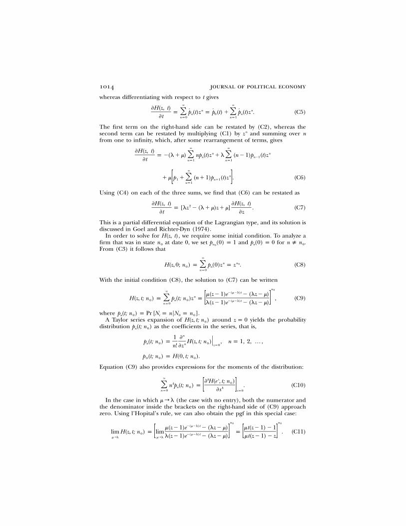
whereas differentiating with respect to t gives� �

�H(z, t) n n˙ ˙ ˙p p (t)z p p (t) � p (t)z . (C5)� �n 0 n�t np0 np1

The first term on the right-hand side can be restated by (C2), whereas thesecond term can be restated by multiplying (C1) by and summing over nnzfrom one to infinity, which, after some rearrangement of terms, gives

� ��H(z, t) n np �(l � m) np (t)z � l (n � 1)p (t)z� �n n�1

�t np1 np1

�

n� m p � (n � 1)p (t)z . (C6)�1 n�1[ ]np1

Using (C4) on each of the three sums, we find that (C6) can be restated as

�H(z, t) �H(z, t)2p [lz � (l � m)z � m] . (C7)�t �z

This is a partial differential equation of the Lagrangian type, and its solution isdiscussed in Goel and Richter-Dyn (1974).

In order to solve for , we require some initial condition. To analyze aH(z, t)firm that was in state at date 0, we set and for .n p (0) p 1 p (0) p 0 n ( n0 n n 00

From (C3) it follows that�

n n0H(z, 0; n ) p p (0)z p z . (C8)�0 nnp0

With the initial condition (C8), the solution to (C7) can be writtenn0

� �(m�l)tm(z � 1)e � (lz � m)nH(z, t; n ) p p (t; n )z p , (C9)�0 n 0 �(m�l)t[ ]l(z � 1)e � (lz � m)np0

where .p (t; n ) p Pr [N p nFN p n ]n 0 t 0 0

A Taylor series expansion of around yields the probabilityH(z, t; n ) z p 00

distribution as the coefficients in the series, that is,p (t; n )n 0

n1 �p (t; n ) p H(z, t; n )F , n p 1, 2, … ,n 0 0n zp0n! �z

p (t; n ) p H(0, t; n ).0 0 0

Equation (C9) also provides expressions for the moments of the distribution:

� k s� H(e , t; n )0kn p (t; n ) p . (C10)� n 0 k[ ]�snp0 sp0

In the case in which (the case with no entry), both the numerator andm r lthe denominator inside the brackets on the right-hand side of (C9) approachzero. Using l’Hopital’s rule, we can also obtain the pgf in this special case:

n n0 0�(m�l)tm(z � 1)e � (lz � m) mt(z � 1) � 1

limH(z, t; n ) p lim p . (C11)0 �(m�l)t[ ] [ ]l(z � 1)e � (lz � m) mt(z � 1) � zmrl mrl


Appendix D

The Size Distribution

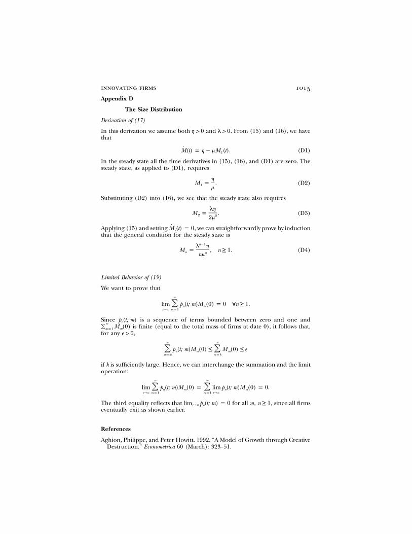
Derivation of (17)

In this derivation we assume both and . From (15) and (16), we haveh 1 0 l 1 0that

M(t) p h � mM (t). (D1)1

In the steady state all the time derivatives in (15), (16), and (D1) are zero. Thesteady state, as applied to (D1), requires

hM p . (D2)1

m

Substituting (D2) into (16), we see that the steady state also requires

lhM p . (D3)2 22m

Applying (15) and setting , we can straightforwardly prove by inductionM (t) p 0n

that the general condition for the steady state isn�1l h

M p , n ≥ 1. (D4)n nnm

Limited Behavior of (19)

We want to prove that�

lim p (t; m)M (0) p 0 Gn ≥ 1.� n mmp1tr�

Since is a sequence of terms bounded between zero and one andp (t; m)n

is finite (equal to the total mass of firms at date 0), it follows that,�� M (0)mmp1

for any ,e 1 0� �

p (t; m)M (0) ≤ M (0) ≤ e� �n m mmpk mpk

if k is sufficiently large. Hence, we can interchange the summation and the limitoperation:

� �

lim p (t; m)M (0) p limp (t; m)M (0) p 0.� �n m n mmp1 mp1tr� tr�

The third equality reflects that for all , since all firmslim p (t; m) p 0 m, n ≥ 1tr� n

eventually exit as shown earlier.

References

Aghion, Philippe, and Peter Howitt. 1992. “A Model of Growth through CreativeDestruction.” Econometrica 60 (March): 323–51.


Amaral, Luıs A. Nunes, Sergey V. Buldyrev, Shlomo Havlin, Michael A. Salinger,and H. Eugene Stanley. 1998. “Power Law Scaling for a System of InteractingUnits with Complex Internal Structure.” Physical Rev. Letters 80 (February 16):1385–88.

Audretsch, David B. 1995. Innovation and Industry Evolution. Cambridge, Mass.:MIT Press.

Barro, Robert J., and Xavier Sala-i-Martin. 1995. Economic Growth. New York:McGraw-Hill.

Bernard, Andrew B., Jonathan Eaton, J. Bradford Jensen, and Samuel Kortum.2003. “Plants and Productivity in International Trade.” A.E.R. 93 (September):1268–90.

Blundell, Richard, Rachel Griffith, and Frank Windmeijer. 2002. “IndividualEffects and Dynamics in Count Data Models.” J. Econometrics 108 (May): 113–31.

Carroll, Glenn R., and Michael T. Hannan. 2000. The Demography of Corporationsand Industries. Princeton, N.J.: Princeton Univ. Press.

Caves, Richard E. 1998. “Industrial Organization and New Findings on the Turn-over and Mobility of Firms.” J. Econ. Literature 36 (December): 1947–82.

Cockburn, Iain M., Rebecca M. Henderson, and Scott Stern. 2000. “Untanglingthe Origins of Competitive Advantage.” Strategic Management J. 21 (October/November): 1123–45.

Cohen, Wesley M. 1995. “Empirical Studies of Innovative Activity.” In Handbookof the Economics of Innovations and Technological Change, edited by Paul Stone-man. Oxford: Blackwell.

Cohen, Wesley M., and Steven Klepper. 1992. “The Anatomy of Industry R&DIntensity Distributions.” A.E.R. 82 (September): 773–99.

———. 1996. “A Reprise of Size and R&D.” Econ. J. 106 (July): 925–51.Cohen, Wesley M., and Richard C. Levin. 1989. “Empirical Studies of Innovation

and Market Structure.” In Handbook of Industrial Organization, vol. 2, edited byRichard Schmalensee and Robert D. Willig. Amsterdam: North-Holland.

Dunne, Timothy, Mark J. Roberts, and Larry Samuelson. 1988. “Patterns of FirmEntry and Exit in U.S. Manufacturing Industries.” Rand J. Econ. 19 (Winter):495–515.

Eaton, Jonathan, and Samuel Kortum. 1999. “International Technology Diffu-sion: Theory and Measurement.” Internat. Econ. Rev. 40 (August): 537–70.

Ericson, Richard, and Ariel Pakes. 1995. “Markov-Perfect Industry Dynamics: AFramework for Empirical Work.” Rev. Econ. Studies 62 (January): 53–82.

Geroski, Paul A. 1998. “An Applied Econometrician’s View of Large CompanyPerformance.” Rev. Indus. Organization 13 (June): 271–94.

Goel, Narendra S., and Nira Richter-Dyn. 1974. Stochastic Models in Biology. NewYork: Academic Press.

Griliches, Zvi. 1979. “Issues in Assessing the Contribution of Research and De-velopment to Productivity Growth.” Bell J. Econ. 10 (Spring): 92–116.

———. 1990. “Patent Statistics as Economic Indicators: A Survey.” J. Econ. Lit-erature 28 (December): 1661–1707.

———. 1995. “R&D and Productivity: Econometric Results and MeasurementIssues.” In Handbook of the Economics of Innovations and Technical Change, editedby Paul Stoneman. Oxford: Blackwell.

———. 1998. R&D and Productivity: The Econometric Evidence. Chicago: Univ. Chi-cago Press (for NBER).

———. 2000. R&D, Education, and Productivity: A Retrospective. Cambridge, Mass.:Harvard Univ. Press.


Grossman, Gene M., and Elhanan Helpman. 1991. Innovation and Growth in theGlobal Economy. Cambridge, Mass.: MIT Press.

Hall, Bronwyn H. 1996. “The Private and Social Returns to Research and De-velopment.” In Technology, R&D, and the Economy, edited by Bruce R. Smithand Claude E. Barfield. Washington, D.C.: Brookings Inst.

Hall, Bronwyn H., Zvi Griliches, and Jerry A. Hausman. 1986. “Patents and Rand D: Is There a Lag?” Internat. Econ. Rev. 27 (June): 265–83.

Hall, Bronwyn H., and Fumio Hayashi. 1989. “Research and Development as anInvestment.” Working Paper no. 2973 (May). Cambridge, Mass.: NBER.

Henderson, Rebecca. 1993. “Underinvestment and Incompetence as Responsesto Radical Innovation: Evidence from the Photolithographic Alignment Equip-ment Industry.” Rand J. Econ. 24 (Summer): 248–70.

Hopenhayn, Hugo A. 1992. “Entry, Exit, and Firm Dynamics in Long Run Equi-librium.” Econometrica 60 (September): 1127–50.

Howitt, Peter. 2000. “Endogenous Growth and Cross-Country Income Differ-ences.” A.E.R. 90 (September): 829–46.

Hymer, Stephen, and Peter Pashigian. 1962. “Firm Size and Rate of Growth.”J.P.E. 70 (December): 556–69.

Ijiri, Yuji, and Herbert A. Simon. 1977. Skew Distributions and the Sizes of BusinessFirms. Amsterdam: North-Holland.

Johnson, Norman L., Samuel Kotz, and Adrienne W. Kemp. 1992. UnivariateDiscrete Distributions. 2d ed. New York: Wiley.

Jones, Charles I. 1995. “R&D-Based Models of Economic Growth.” J.P.E. 103(August): 759–84.

Jovanovic, Boyan. 1982. “Selection and the Evolution of Industry.” Econometrica50 (May): 649–70.

———. 1993. “The Diversification of Production.” Brookings Papers Econ. Activity:Microeconomics, pp. 197–247.

———. 2001. “Fitness and Age: Review of Carroll and Hannan’s Demography ofCorporations and Industries.” J. Econ. Literature 39 (March): 105–19.

Karlin, Samuel, and Howard Taylor. 1975. A First Course in Stochastic Processes. 2ded. San Diego: Academic Press.

Kendall, David G. 1948. “On the Generalized ‘Birth-and-Death’ Process.” Ann.Math. Statis. 19 (March): 1–15.

Kleinknecht, Alfred. 1987. “Measuring R&D in Small Firms: How Much Are WeMissing?” J. Indus. Econ. 36 (December): 253–56.

Klepper, Steven. 1996. “Entry, Exit, Growth, and Innovation over the ProductLife Cycle.” A.E.R. 86 (June): 562–83.

Klepper, Steven, and Peter Thompson. 2002. “Submarkets and the Evolution ofMarket Structure.” Manuscript. Pittsburgh: Carnegie Mellon Univ.

Klette, Tor Jakob. 1996. “R&D, Scope Economies, and Plant Performance.” RandJ. Econ. 27 (Autumn): 502–22.

Klette, Tor Jakob, and Zvi Griliches. 1996. “The Inconsistency of Common ScaleEstimators When Output Prices Are Unobserved and Endogenous.” J. Appl.Econometrics 11 (July–August): 343–61.

———. 2000. “Empirical Patterns of Firm Growth and R&D Investment: A Qual-ity Ladder Model Interpretation.” Econ. J. 110 (April): 363–87.

Klette, Tor Jakob, and Frode Johansen. 1998. “Accumulation of R&D Capitaland Dynamic Firm Performance: A Not-So-Fixed Effect Model.” Ann.d’Economie et de Statistique, nos. 49/50 (January/June), pp. 389–419.

Kortum, Samuel S. 1997. “Research, Patenting, and Technological Change.”Econometrica 65 (November): 1389–1419.


Langlois, Richard N., and Paul L. Robertson. 1995. Firms, Markets and EconomicChange: A Dynamic Theory of Business Institutions. New York: Routledge.

Li, Chol-Won. 2001. “On the Policy Implications of Endogenous TechnologicalProgress.” Econ. J. 111 (May): C164–C179.

Lucas, Robert E., Jr. 1967. “Adjustment Costs and the Theory of Supply.” J.P.E.75, no. 4, pt. 1 (August): 321–34.

Lucas, Robert E., Jr., and Edward C. Prescott. 1971. “Investment under Uncer-tainty.” Econometrica 39 (September): 659–81.

Mansfield, Edwin. 1986. “The R&D Tax Credit and Other Technology PolicyIssues.” A.E.R. Papers and Proc. 76 (May): 190–94.

Nelson, Richard R. 1988. “Modelling the Connections in the Cross Section be-tween Technical Progress and R&D Intensity.” Rand J. Econ. 19 (Autumn):478–85.

Penrose, Edith T. 1959. The Theory of the Growth in the Firm. Oxford: Blackwell.Peretto, Pietro F. 1999. “Cost Reduction, Entry, and the Interdependence of

Market Structure and Economic Growth.” J. Monetary Econ. 43 (February):173–95.

Romer, Paul M. 1990. “Endogenous Technological Change.” J.P.E. 98, no. 5, pt.2 (October): S71–S102.

Schmalensee, Richard. 1989. “Inter-industry Studies of Structure and Perfor-mance.” In Handbook of Industrial Organization, vol. 2, edited by Richard Schma-lensee and Robert D. Willig. Amsterdam: North-Holland.

Scott, John T. 1984. “Firm versus Industry Variability in R&D Intensity.” In R&D,Patents, and Productivity, edited by Zvi Griliches. Chicago: Univ. Chicago Press(for NBER).

Segerstrom, Paul S. 1998. “Endogenous Growth without Scale Effects.” A.E.R.88 (December): 1290–1310.

Simon, Herbert A., and Charles P. Bonini. 1958. “The Size Distribution of Busi-ness Firms.” A.E.R. 48 (September): 607–17.

Stanley, Michael H. R., et al. 1995. “Zipf Plots and the Size Distribution of Firms.”Econ. Letters 49 (October): 453–57.

Sutton, John. 1997. “Gibrat’s Legacy.” J. Econ. Literature 35 (March): 40–59.———. 1998. Technology and Market Structure: Theory and History. Cambridge,

Mass.: MIT Press.———. 2002. “The Variance of Firm Growth Rates: The ‘Scaling’ Puzzle.” Physica

A 312 (September 15): 577–90.Thompson, Peter. 1996. “Technological Opportunity and the Growth of Knowl-

edge: A Schumpeterian Approach to Measurement.” J. Evolutionary Econ. 6(February): 77–97.

———. 2001. “The Microeconomics of an R&D-Based Model of EndogenousGrowth.” J. Econ. Growth 6 (December): 263–83.

Thompson, Peter, and Doug Waldo. 1994. “Growth and Trustified Capitalism.”J. Monetary Econ. 34 (December): 445–62.

Uzawa, Hirofumi. 1969. “Time Preference and the Penrose Effect in a Two-ClassModel of Economic Growth.” J.P.E. 77, no. 4, pt. 2 (July/August): 628–52.

innovating firms and aggregate innovationweb.stanford.edu/~klenow/klette and kortum.pdf · ·...

Documents