input force identification: application to soil–pile interaction

STRUCTURAL CONTROL AND HEALTH MONITORING

Struct. Control Health Monit. 2009; 16:223–240Published online 19 December 2008 in Wiley InterScience(www.interscience.wiley.com). DOI: 10.1002/stc.308

Input force identification: Application to soil–pile interaction

Ai-Lun Wu1,z, Chin-Hsiung Loh1,�,y,y, Jann N. Yang2,y, Jian-Huang Weng1,z,Chia-Han Chen1,z and Tzou-Shin Ueng1,y

1Department of Civil Engineering, National Taiwan University, Taipei 106-17, Taiwan2Department of Civil and Environmental Engineering, University of California, Irvine, CA 92697, U.S.A.

SUMMARY

An identification method for estimating the time varying excitation force acting on a structuralsystem based on its response measurements is presented in this study. The method employs the simpleKalman filter to establish a regression model between the residual innovation and the input excitationforces. In applying the method, first, the ambient vibration measurement of a structural system is collected,then the stochastic subspace identification is applied to estimate the system matrix ‘A’ and themeasurement matrix ‘H ’. Incorporated with the identified ‘A’ and ‘H ’ matrices the dynamic excitationforces are estimated from the measured structural responses by using Kalman filter with a recursiveleast-square estimator to update the estimation in the sense of real-time computation. Verification of themethod on numerical simulation through MIMO system is conducted first. Identification of soil forcesduring the shaking table test of soil–pile interaction is also demonstrated. Copyright r 2008 John Wiley &Sons, Ltd.

KEY WORDS: Kalman filter estimation; recursive least square; soil–pile interaction; stochastic subspaceidentification

INTRODUCTION

Accurate estimation of input excitation forces acting on a structure is significant for designing,controlling and diagnosing a structural system. Prior knowledge of accurate input excitation

*Correspondence to: Chin-Hsiung Loh, Department of Civil Engineering, National Taiwan University, Taipei 106-17,Taiwan.yE-mail: [email protected] Assistant.yProfessor.zGraduate Student.

Contract/grant sponsor: Excellent Research Funds; contract/grant number: 95R0066-BE03-06Contract/grant sponsor: National Science Council; contract/grant number: NSC 96-2221-E-002-121-MY3

Copyright r 2008 John Wiley & Sons, Ltd.

Received 22 February 2008Revised 7 November 2008

Accepted 12 November 2008

forces can contribute to a greater reliability of structural safety particularly in the numericalsimulation of designing stage and to reduce the expensive costs for time-consumingexperimental tests. Besides, the input force information can provide important message fordeveloping the damage prognosis model of structures. In some circumstances, input excitationforces can be directly measured using load or acceleration transducers. However, for somephysical and mechanical systems, direct measurements of input excitation forces are difficult tobe realized due to very large magnitudes of input forces or installation obstacle of loadtransducers or the complex interaction between loading and structural response. Therefore, analternate inverse method is needed to reconstruct input excitation forces based upon themeasured structural responses.

Conventional inverse method for input excitation forces are well known as ade-convolution problem from either time domain or frequency domain. The objective ofthe conventional inverse method is to de-convolve the matrix equation to produce an estimateof an input forces based on the structural response and the impulse response. For fields ofseismic and signal processing, a great deal of researches have been applied to solve theconvolution matrix equation in time domain using methods including least-squares, Wienerfiltering and Wavelet de-convolution [1]. However, it is well known that the conventionalinverse method generally tends to represent an ill-posed problem because small changes inmeasurement data can contribute to large changes in the estimate of input excitation forces.Disturbances of measurement data affect the results of input excitation forces. To treat the ill-condition problems, some regularization techniques have been demonstrated. Busby andTrujillo [2] used the least-squares minimization with regularization (Tikhonov method) byadding a term to smooth and stabilize the solutions, while Kammer [3] proposed aregularization technique with Markov parameters to produce an estimate of the correspondinginput excitation forces.

In addition to the conventional inverse method, the Kalman filter-based tracking approachhas been studied and developed for the identification of input excitation forces due to itsaccurate estimation in the consideration of measurement noise and modeling error. Singer [4]augmented the Kalman filter with the target acceleration equation represented by a first-orderautoregressive process. Chan et al. [5] proposed a Kalman filter-based tracking scheme withinput estimation and used a detector to guard against automatic updating of the simpleKalman filter. Ma [6] proposed an application of the Kalman filter to determine the impulseloads of a lumped-mass system in a numerical scheme. Liu et al. [7] used the Kalman filterand least-squares estimator to determine the input excitations of a cantilever plate. Theefficiency and robustness of this proposed algorithm using the Kalman filter and recursiveleast squares with a regularization scheme were proven to be better than the conventionalmethods [8].

In this study, the Kalman filter and recursive least-squares estimator originally proposedby Liu et al. [7] is used. The relationship between the residual innovation and theinput excitation forces are estimated using the Kalman filter estimation, and then based onthe measured structural responses while least-squares method with a recursive estimatoris also employed to update the estimation in the sense of real-time computation. Applicationof the proposed approach will be conducted through a numerical simulation and anexperiment of soil–pile interaction. To improve the accuracy of the input force estimationthe stochastic subspace identification technique was used to estimate the system matrix as aprior.

A.-L. WU ET AL.224

Copyright r 2008 John Wiley & Sons, Ltd. Struct. Control Health Monit. 2009; 16:223–240

DOI: 10.1002/stc

THEORETICAL BACKGROUND

State equations of the system

Consider an n degree-of-freedom lumped-mass system, the equation of motion can be written asfollows:

M €YðtÞ þ C _YðtÞ þ KYðtÞ ¼ FðtÞ ð1Þ

where M denotes the n� n mass matrix, C is the n� n damping matrix, K is the n� n stiffnessmatrix, F(t) is the n� 1 input force vector, €YðTÞ, _YðtÞ and YðtÞ are n� 1 vectors of acceleration,velocity and displacement, respectively. To estimate the states of linear system through theKalman filter, the transformation of the equations of motion is performed. The dynamic systemwith n degree-of-freedom will be represented by 2n� 1 state vectors: XðtÞ ¼ ½YðtÞ _YðtÞ�. Thediscrete-time state and measurement equations can then be written as follows:

Xðkþ 1Þ ¼ AXðkÞ þ BFðkÞ þ GwðkÞ ð2Þ

and

ZðkÞ ¼ HXðkÞ þ vðkÞ ð3Þ

where

A ¼ expðAcDtÞ; B ¼Z Dt

0

eAt dtBc ð4Þ

and H is the measurement matrix, Z(k) denotes the measured observation vector, and

Ac ¼0n�n In�n�M�1K �M�1C

� �; Bc ¼

0n�nM�1

� �ð5aÞ

XðkÞ ¼ ½X1ðkÞ X2ðkÞ . . . X2n�1ðkÞ X2nðkÞ �T ð5bÞ

FðkÞ ¼ ½F1ðkÞ F2ðkÞ F3ðkÞ . . . FnðkÞ �T ð5cÞ

ZðkÞ ¼ ½Z1ðkÞ Z2ðkÞ Z3ðkÞ . . . ZnðkÞ �T ð5dÞ

Equation (2) is discretized over time interval of length Dt, and associated with process noiseinvolving statistical description of the system noise and uncertainty in the dynamic models, andX(k) represents the state vector, A is the state transition matrix, B is the input matrix, Dt is thesampling interval, F(k) is the sequence of the deterministic input, and w(k) is the noise vectorwhich is assumed to be zero mean and white with variance E½wðkÞwTð jÞ� ¼ Qdkj , where Q is theprocess noise covariance matrix and dkj is the Kronecker delta. Z(k) denotes the observationvector and v(k) represents the measurement noise vector. In addition, v(k) is assumed to be zeromean and white noise. The variance of v(k) is given by E½vðkÞvTð jÞ� ¼ Rdkj, where R is themeasurement noise covariance matrix.

The recursive input estimation approach

The Kalman filter and a recursive least-squares algorithm will be used for unknown input forceidentification. The Kalman filter, which is the implementation of a predictor-corrector typeestimator, is optimal in the sense that it minimizes the estimated error covariance when somepresumed conditions are met. The procedure for the traditional estimation of the Kalman filteris shown in Table I. The second part of input force identification is to establish a recursive

INPUT FORCE IDENTIFICATION 225


DOI: 10.1002/stc

relationship between a residual innovation resulting from the Kalman filter and the inputexcitation forces. Considering input excitation forces in a specific time interval:

FðkÞ; k ¼ 1; 2; . . . ; n ð6Þ

Based on the concept provided by Ma et al. [6, 8], procedures for the input force identificationare derived in more detail.

First, a recursive relationship between a residual innovation resulting from the Kalman filterand input excitation force was provided. Let Xðk=kÞ and Xðk=kÞ; respectively, denote thepredicted state X(k) with and without input excitation forces F(k�1). The updated stateestimation without inputs can be expressed as

Xðk=kÞ ¼ Xðk=k� 1Þ þ KaðkÞZðkÞ

¼ Xðk=k� 1Þ þ KaðkÞ½ZðkÞ �HXðk=k� 1Þ�

¼ ½I �HKaðkÞ�Xðk=k� 1Þ þ KaðkÞZðkÞ

¼ ½I �HKaðkÞ�AXðk� 1=k� 1Þ þ KaðkÞZðkÞ

ð7Þ

And the updated state estimation with input can be expressed as

Xðk=kÞ ¼ Xðk=k� 1Þ þ KaðkÞZðkÞ

¼ Xðk=k� 1Þ þ KaðkÞ½ZðkÞ �HXðk=k� 1Þ�

¼ ½I �HKaðkÞ�½Xðk=k� 1Þ� þ KaðkÞZðkÞ

¼ ½I �HKaðkÞ�½AXðk� 1=k� 1Þ þ BF � þ KaðkÞZðkÞ

ð8Þ

Second, the difference between Xðk=kÞ and Xðk=kÞ was defined. It is now defined as

DXðk=kÞ ¼ Xðk=kÞ � Xðk=kÞ

¼ ½I �HKaðkÞ�½AðXðk� 1=k� 1Þ � Xðk� 1=k� 1ÞÞ þ BF �

¼ ½I �HKaðkÞ�½ADXðk� 1=k� 1Þ þ BF �

ð9Þ

From Equation (9), DXðk=kÞ can be assumed as [9]

DXðk=kÞ ¼MsðkÞBF ð10Þ

Substitute Equation (10) into Equation (9), the recursive form of Ms(k) can be derived.

Table I. Traditional Kalman filter estimation procedures.

1. State prediction Xðk=k� 1Þ ¼ AXðk� 1=k� 1Þ2. State prediction covariance Pðk=k� 1Þ ¼ APðk� 1=k� 1ÞAT þ BQBT

3. Calculate innovation covariance SðkÞ ¼ HPðk=k� 1ÞHT þ R

4. Estimate Kalman gain KaðkÞ ¼ Pðk=k� 1ÞHTS�1ðkÞ5. Updated state covariance Pðk=kÞ ¼ ½I � KaðkÞH�Pðk=k� 1Þ6. Calculate innovation ZðkÞ ¼ ZðkÞ �HXðk=k� 1Þ7. Updated state estimation Xðk=kÞ ¼ Xðk=k� 1Þ þ KaðkÞZðkÞ

A.-L. WU ET AL.226


DOI: 10.1002/stc

Therefore,

MsðkÞBF ¼ ½I �HKaðkÞ�½AMsðk� 1ÞBF þ BF �

¼ ½I �HKaðkÞ�½AMsðk� 1Þ þ I �BF

MsðkÞ ¼ ½I �HKaðkÞ�½AMsðk� 1Þ þ I �

ð11Þ

The relationship between the two estimations is expressed as

Xðk=kÞ ¼ Xðk=kÞ þMsðkÞBF

MsðkÞ ¼ ½I � KaðkÞH�½AMsðk� 1Þ þ I �ð12Þ

where Third, let ZðkÞ and ZðkÞ denote the innovation Z(k) with and without input excitationforces F(k�1), respectively. The difference between ZðkÞ and ZðkÞ can be expressed as

ZðkÞ � ZðkÞ ¼ HAXðk� 1=k� 1Þ �HAXðk� 1=k� 1Þ þHBF

¼ HA½Xðk� 1=k� 1Þ � Xðk� 1=k� 1Þ� þHBF

¼ H½AMsðk� 1ÞBF � þHBF

¼ H½AMsðk� 1Þ þ I �BF

ð13Þ

Therefore, the difference between ZðkÞ and ZðkÞ can be expressed as

ZðkÞ ¼ ZðkÞ þ BsðkÞF ð14Þ

where

Bs ¼ HðAMsðk� 1Þ þ IÞB

Consider time step k ¼ m;mþ 1; . . . ;mþ n, Equation (14) can be rewritten as

<ðNÞ ¼ BsðNÞF þ EðNÞ ð15Þ

where

<ðNÞ ¼ ½Zðmþ 1Þ Zðmþ 2Þ . . . Zðmþ nÞ �T

EðNÞ ¼ ½ Zðmþ 1Þ Zðmþ 2Þ . . . Zðmþ nÞ �T

BsðNÞ ¼

Bsðmþ 1Þ

Bsðmþ 2Þ

..

.

Bsðmþ nÞ

26666666664

37777777775¼

HB

HðAMsðmþ 1Þ þ IÞB

..

.

HðAMsðmþ n� 1Þ þ IÞB

26666666664

37777777775

ð16Þ



DOI: 10.1002/stc

From this equation, EðNÞ can be treated as a disturbance vector, whose covariance L(N) can bedenoted as:

LðNÞ ¼

Sðmþ 1Þ 0 � � � 0

0 Sðmþ 2Þ � � � 0

..

. ... . .

. ...

0 0 � � � Sðmþ nÞ

26666664

37777775

ð17Þ

where

SðkÞ ¼ E ½ZðkÞZðkÞ� ¼ HPðk=k� 1ÞHT þ R ð18Þ

Equation (15) provides the recursive relationship between the residual innovation and the inputexcitation forces. Therefore, a least-squares algorithm [10] is employed to solve thecorresponding input loads and the result in a batch form can be obtained as follows:

FðNÞ ¼ ½BTs ðNÞL

�1ðNÞBsðNÞ��1BTs ðNÞL

�1ðNÞ<ðNÞ ð19Þ

And the error covariance is

PbðNÞ ¼ E ½ðF � FðNÞÞðF � FðNÞÞT� ¼ ½BTs ðNÞL

�1ðNÞBsðNÞ��1 ð20Þ

The regression model for time step k ¼ m;mþ 1; . . . ;mþ n has been derived. Then, consideringnext time step k5m1n11, one can obtain that

<ðN þ 1Þ ¼ BsðN þ 1ÞF þ EðN þ 1Þ ð21Þ

where

<ðN þ 1Þ ¼<ðNÞ

ZðN þ 1Þ

" #; BsðN þ 1Þ ¼

BsðNÞ

BsðN þ 1Þ

" #

EðN þ 1Þ ¼EðNÞ

ZðN þ 1Þ

" #; L�1ðN þ 1Þ ¼

gL�1ðNÞ 0

0 s�1ðN þ 1Þ

24

35 ð22Þ

The forgetting factor g is used in Equation (22). Then

FðN þ 1Þ ¼ ½BTs ðN þ 1ÞL�1ðN þ 1ÞBsðN þ 1Þ��1BT

s ðN þ 1ÞL�1ðN þ 1Þ<ðN þ 1Þ ð23Þ

PbðN þ 1Þ ¼ ½BTs ðN þ 1ÞL�1ðN þ 1ÞBsðN þ 1Þ��1

¼ ½g�1P�1b ðNÞ þ BTs ðN þ 1ÞL�1ðN þ 1ÞBSðN þ 1Þ��1

ð24Þ

Substituting Equation (22) into Equation (23) and applying matrix inversion lemma, theimplementation of the recursive least-squares algorithm can be obtained. The equations of therecursive least-squares algorithm are summarized in Table II. In summary, the input excitationforces can be estimated through the following steps:

(1) Using system identification techniques to derive the system model and measure thedynamic responses of system.

A.-L. WU ET AL.228


DOI: 10.1002/stc

(2) Using the Kalman filter equations to obtain the innovation covariance S(k), innovationZðkÞ and Kalman gainKaðkÞ.

(3) Using the recursive least-squares algorithm to estimate the input forces FðkÞ.

NUMERICAL EXAMPLE: VERIFICATION

The implementation of the proposed approach is verified by using data from a simulation of athree degree-of-freedom system subjected to three input forces at each degree-of-freedom. Athree degree-of-freedom-system, as shown in Figure 1, with input excitation at each node (orlumped mass) is assigned and the response from each node is calculated. The equation of motionof the system is expressed as

m1 0 0

0 m2 0

0 0 m3

2664

3775

€x1

€x2

€x3

8>><>>:

9>>=>>;þ

2c �c 0

�c 2c �c

0 �c 2c

2664

3775

_x1

_x2

_x3

8>><>>:

9>>=>>;þ

2k �k 0

�k 2k �k

0 �k 2k

2664

3775

x1

x2

x3

8>><>>:

9>>=>>; ¼

F1

F2

F3

8>><>>:

9>>=>>;ð25Þ

To conduct the input force identification, the mass, damping as well as stiffness matrices of thesystem are assumed as known matrices (as shown below):

M ¼

6:11 0 0

0 6:11 0

0 0 6:11

264

375 kg; C ¼

10 �5 0

�5 10 �5

0 �5 10

264

375Ns=m

K ¼

3600 �1800 0

�1800 3600 �1800

0 �1800 3600

264

375N=m

F2

m1 m2 m3

k k k k

F1

c c c c

Figure 1. Three degree-of-freedom systems.

Table II. Recursive least-squares algorithms for input force identification.

1. Sensitivity matrices BsðkÞ ¼ H½AMsðk� 1Þ þ I �B andMsðkÞ ¼ ½I � KaðkÞH�½AMsðk� 1Þ þ I �

2. Correction gain for the updatinginput forces vector

KbðkÞ ¼ g�1Pbðk� 1ÞBTs ðkÞ½BsðkÞg�1

Pbðk� 1ÞBTs ðkÞ þ SðkÞ��1

3. Error covariance of the estimatedinput forces vector

PbðkÞ ¼ ½I � KbðkÞBsðkÞ�g�1Pbðk� 1Þ

4. Estimated input forces vector FðkÞ ¼ Fðk� 1Þ þ KbðkÞ½ZðkÞ � BsðkÞFðk� 1Þ�



DOI: 10.1002/stc

Two different response simulations are conducted. One is the low-level white noise excitationand the other is the force excitation. The white noise response will be used for systemidentification and the response from the force excitation will be used for input forceidentification. The force is applied at the lumped mass. Acceleration response (with 10% RMSwhite noise was added on the response data) from each degree-of-freedom is measured.

The following two steps are used for input force identification:(1) Using SSI method (output only) to identify the system matrix ‘A’ and ‘H ’: Using a set of

input/output data of the system, for example, the responses of white noise excitation, theoutput-only SSI method is applied to identify the system matrix ‘A’ and the response matrix‘H’ (in the state space equation). These ‘A’ and ‘H ’ matrices will be used for input forceidentification. It is important to note that the prior knowledge of system matrix ‘A’ and ‘H ’matrices is required for input force identification. Based on the provided system matrix ‘A’matrix, the identified three dominant frequencies of the system are 2.08, 3.86 and 5.04Hz,respectively. It has to point out that if only output signals are collected, then the systemmatrix ‘A’ and the measurement matrix ‘H ’ can be identified from output-only SSI method.Therefore, the amplitude of the identified input forces cannot be estimated correctivelybecause of unknown ‘B’ matrix. On the contrary, if the both input and output signals aremeasured, then the system matrix ‘A’, the measurement matrix ‘H ’ and the input matrix ‘B’can be identified by using the input/output SSI method. Therefore, the input force can beidentified correctively.

(2) Adapt Kalman filter with recursive least square for input force identification: In thissimulation it is assumed that a set of noise-contaminated acceleration response data is collectedfrom all the degree-of-freedom of the system. Based on the proposed method and the identified‘A’, ‘B’ and ‘H’ matrices the input force can be identified. Figure 2 shows the comparison

-100

0

100

N

0 1 2 3 4 5 6 7 8

0 1 2 3 4 5 6 7 8

0 1 2 3 4 5 6 7 8

-200

0

200

-200

0

200

time (sec)

CH3

CH2

CH1

Figure 2. Comparison on the input excitations between the actual and the identified forces (dark line:numerical simulation; light line: estimated input excitation).

A.-L. WU ET AL.230


DOI: 10.1002/stc

between the identified and actual input excitations. The waveform and the amplitudes of theidentified input force are quite in consistent with the simulation. Because the response data arenoise-contaminated, the identified force is not in close consistent with the exact input force.

IDENTIFICATION OF SOIL FORCE FROM SOIL–PILE INTERACTION

Bridge piers are normally supported on piles driven through a deep layer of relatively weakmaterial to a penetration in the underlying firm material deemed sufficient to carry thesuperimposed loads by friction or by point bearing. To design a pile subjected to earthquakeexcitation the soil–pile interaction needs to be considered. Force acting on the pile duringearthquake excitation can be identified from the proposed method. Referring to Figure 3, theidealized model of the soil–pile interaction system will be excited at its base by the prescribedhorizontal acceleration €ug of the foundation medium and at each level i ði ¼ 1; 2; . . . ; nÞ by aknown support acceleration time history. Let €uti represents the acceleration time history of theclay medium at level i assuming no interaction with the soil–pile interaction. The differentialequation of motion of the soil–pile interaction that governs the response of this idealizedstructural system is shown as follows: [11]:

Mi €uri þ ci _u

Si � ciþ1 _u

Siþ1 þ kiu

Si � kiþ1u

Siþ1 þ FS

i ðtÞ ¼ �Mi €ugðtÞ þmei €u

ti ð26Þ

where uri is the motion of mass Mi w.r.t. the base, €ug is the base ground motion, uti is the far-fieldground motion of clay material assuming no interaction, uSi is the relative motion between twolumped masses, FS

i is the interaction force between clay medium and pile resulting from therelative motion caused by interaction, me

i is the the effective mass of clay medium resulting fromits interaction with the pile. The horizontal forces include in the above equation are inertia,damping and transverse shear, effective seismic load. The identification of the interaction force

Mi-1

Mi+1

Mi

usi+1

Fixed reference

ug

uit

uis

Figure 3. Idealized model of the soil–pile interaction system.



DOI: 10.1002/stc

between clay medium and pile resulting from the relative motion caused by interaction is themajor task of this research.

To investigate the soil–pile interaction forces during earthquake excitation, a shaking tabletest of the soil–pile interaction was conducted. A hollow steel pipe, representing the pile, isburied in the shear box filled with soil, as shown in Figure 4. The instrumentation in thissoil–pile interaction test is shown in Figure 5. In this study only acceleration responses along thepipe and in the far-field (no effect on interaction) are used to identify the interaction forces. TheARX model was first used to identify the natural frequency of the pile itself by using the datafrom the white noise excitation. The first fundamental natural frequency of the pipe is 13.7Hz.The lumped mass model of the pile system is also generated, so that the proposed method can beapplied directly. It is assumed that a five degree-of-freedom system is selected to represent thesoil–pile interaction system. Figure 6 shows the continuous and the discrete model of the system.

Figure 4. Schematic diagram of the soil–pile system in shear box for shaking table test.

A.-L. WU ET AL.232


DOI: 10.1002/stc

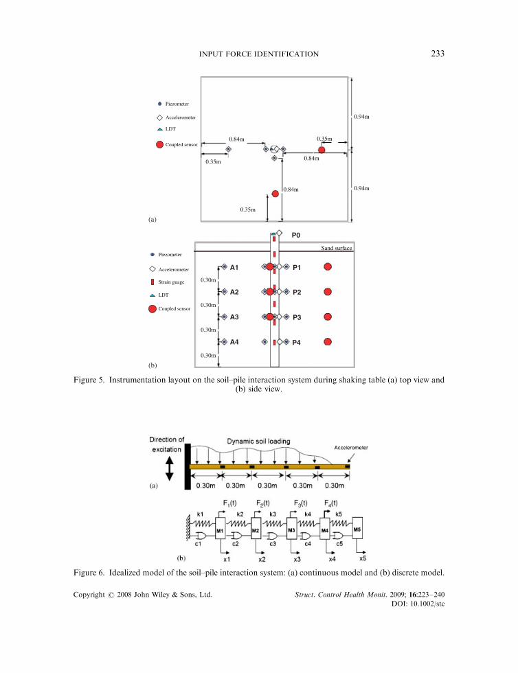
Figure 6. Idealized model of the soil–pile interaction system: (a) continuous model and (b) discrete model.

(a)

A1

A2

A3

A4

P0

P1

P2

P3

P4

Piezometer

Accelerometer

Piezometer

Accelerometer

Strain guage

LDT

Coupled sensor

LDT

0.84m

0.84m

0.84m

0.35m

0.35m

0.30m

0.30m

0.30m

0.30m

0.35m

0.94m

0.94m

Sand surface

Coupled sensor

(b)

Figure 5. Instrumentation layout on the soil–pile interaction system during shaking table (a) top view and(b) side view.



DOI: 10.1002/stc

The equation of motion of the 5-DOFs discrete system is shown as

M1 0 0 0 0

0 M2 0 0 0

0 0 M3 0 0

0 0 0 M4 0

0 0 0 0 M5

2666664

3777775

€u1€u2€u3€u4€u5

8>>>>><>>>>>:

9>>>>>=>>>>>;þ

c11 c12 c13 c14 c15

c21 c22 c23 c24 c25

c31 c32 c33 c34 c35

c41 c42 c43 c44 c45

c51 c52 c53 c54 c55

2666664

3777775

_u1_u2_u3_u4_u5

8>>>>><>>>>>:

9>>>>>=>>>>>;

þ

k11 k12 k13 k14 k15

k21 k22 k23 k24 k25

k31 k32 k33 k34 k35

k41 k42 k43 k44 k45

k51 k52 k53 k54 k55

2666664

3777775

u1

u2

u3

u4

u5

8>>>>><>>>>>:

9>>>>>=>>>>>;þ

F1

F2

F3

F4

F5

8>>>>><>>>>>:

9>>>>>=>>>>>;

¼ �

M1 0 0 0 0

0 M2 0 0 0

0 0 M3 0 0

0 0 0 M4 0

0 0 0 0 M5

2666664

3777775 €ug þ

me1 0 0 0 0

0 me2 0 0 0

0 0 me3 0 0

0 0 0 me4 0

0 0 0 0 me5

8>>>>><>>>>>:

9>>>>>=>>>>>;

€ut1€ut2€ut3€ut4€ut5

8>>>>><>>>>>:

9>>>>>=>>>>>;

or

M €uþ C _uþ Kuþ FS ¼ �M €ug þMe €ut ð27Þ

where u(t) is the relative displacement with respect to base. The properties, including mass,damping and stiffness matrices, determined from finite element model and verified throughexperimental testing result of the pile, are as shown below:

M ¼

2:18 0 0 0 0

0 2:18 0 0 0

0 0 2:18 0 0

0 0 0 2:18 0

0 0 0 0 19:09

2666664

3777775 10�3kN� s2=m

C ¼

1:89 �1:09 0:28 0:02 �0:01

�1:09 1:54 �1:07 0:31 �0:02

0:28 �1:07 1:57 �1:06 0:27

0:02 0:31 �1:06 1:23 �0:47

�0:01 �0:02 0:27 �0:47 0:26

2666664

3777775 kN� s=m

K ¼

6:88 �3:98 1:05 0:07 �0:07

�3:98 5:63 �3:91 1:15 �0:07

1:05 �3:91 5:72 �3:89 1:02

0:07 1:15 �3:89 4:49 �1:73

�0:07 �0:07 1:02 �1:73 0:81

2666664

3777775 104kN=m

During the shaking table test of soil–pile interaction study, €u; €ug; €ut are the measured signals.

A.-L. WU ET AL.234


DOI: 10.1002/stc

Equation (27) is first modified and expressed as

M €uþ C _uþ Ku ¼ �F �M €ug þMe €ut ¼ Ftotal ð28Þ

where Ftotal is the summation of three forces: the interaction force between clay medium andpile, M €ug is the earthquake loading and Me €ut is the far-field soil inertia force. Application of theproposed method on the input force identification of the soil–pile interaction is conducted. Ftotal

can be identified using the Kalman filter and recursive least estimator. Figure 7 shows therecorded accelerations from the acceleration sensors along the pile during testing and Figure 8shows the identified input force of soil–pile interaction. In the discrete model of the pile there isno interaction force acting at nodal point 5 (M5). Therefore, only forces acting from nodal pointone to nodal point four have the interaction force.

Comparison between the identified input force and the recorded far-field acceleration,recorded acceleration along the pile and the identified input force at level of 120 cm is plottedand shown in Figure 9. The wavelet packet transform (WPT) is applied to these records as wellas the estimated input force time history so as to identify the differences among them [12]. TheWPT is employed to level 9 by using Bio (6.8) mother wavelet [13]. From WPT analysis eachcomponent of energy is calculated. Figure 10 shows the distribution of percentage of waveletcomponent energy of the far-field acceleration, recorded pile acceleration, identified inputforce and the input ground acceleration. It is found that the percentage of component energyof the identified soil–pile interaction force is very significant, particularly in the frequency

0

50

100

0

50

100

0

50

100

Am

plitu

de

0

50

100

0 5 10 15 20 25

0 5 10 15 20 25

0 5 10 15 20 25

0 5 10 15 20 25

0 5 10 15 20 25

0

50

100

Hz

P0

P1

P2

P3

P4

0 20 40 60 80 100-0.5

0

0.5

0 20 40 60 80 100-0.5

0

0.5

0 20 40 60 80 100-0.5

0

0.5

0 20 40 60 80 100-0.5

0

0.5

0 20 40 60 80 100-0.5

0

0.5

time (sec)

P0

P1

P2

P3

P4

Acc

eler

atio

n (g

)

Figure 7. Recorded acceleration time history (unit: g) and the corresponding Fourier amplitude spectrumfrom the measurement along the pile from the shaking table test.



DOI: 10.1002/stc

range of 13.7Hz, which is consist with the natural frequency of the pile. Since the identifiedinput force consists of three terms, soil–structural interaction force, input excitation and theeffective mass of soil medium (Ftotal ¼ �F �M €ug þMe €ut), and the frequency contents of inputexcitation and the effective mass of soil medium are all below 10.0Hz, therefore, the frequencycontents of the interaction force between clay medium and pile are focus around the peripheryof the natural frequency of the pile.

A simulation of MDOF elastic system subjected to earthquake excitation will be demonstratedto identify the elastic forces of structure as a comparison to the prior soil–pile interaction forces.The relative-response equation of motion of a lumped MDOF system can be denoted as

M €uþ C _uþ Ku ¼ Peff ðtÞ ð29Þ

in which

PeffðtÞ ¼ �mf1g €ugðtÞ ð30Þ

Therefore, the transformation to normal coordinates can be described as a set of N uncoupledmodal equations:

Mn€Yn þ CnYn þ KnYn ¼ Pn ð31Þ

in which Mn, Cn and Kn are the generalized properties associated with mode n, Yn is theamplitude of modal response, and the generalized force resulting from the earthquake excitationis given by

Pn ¼ fTn Peff ¼ Ln €ugðtÞ ð32Þ

-0.01

0

0.01

-0.01

0

0.01

-0.01

0

0.01

0 20 40 60 80 100

0 20 40 60 80 100

0 20 40 60 80 100

0 20 40 60 80 100

-0.01

0

0.01

time (sec)

P4

P3

P2

P1

0

1

2P1

0

1

2

Am

plitu

de P2

0

1

2P3

0 5 10 15 20 25

0 5 10 15 20 25

0 5 10 15 20 25

0 5 10 15 20 25

0

1

2

Hz

P4

Inpu

t For

ce (

kN)

Figure 8. Identified input force along the pile (at each of the lumped mass) and its corresponding Fourieramplitude spectrum.

A.-L. WU ET AL.236


DOI: 10.1002/stc

in which

Ln � fTnmf1g ð33Þ

is denoted as the modal earthquake-excitation factor. Therefore, the expression of elastic forcesof the system can be derived and described as following [14]:

FsðtÞ ¼ mULn

MnonUnðtÞ

� �ð34Þ

in which U is made up of all mode shapes for which the modal response is excited by earthquake,and the term in the braces represents the response defined for each mode considered in theanalysis.

To examine the phenomenon of soil–pile interaction, the identified force from soil–pile testat the elevation¼120 cm was further processed. Since the identified force was inherentcomposed of three terms, namely the interaction force due to the soil–pile interaction, theinertial force resulted from translation excitation and the effective mass of soil medium(Ftotal ¼ �F �M €ug þMe €ut), eliminating the translation excitation effect can help one realizethe contribution of the rest two terms (Fremove�EQ ¼ �F þMe €ut), and sophisticatedly

-0.25

-0.2

-0.15

-0.1

-0.05

0

0.05

0.1

0.15g

Far-field acceleration

-0.3

-0.2

-0.1

0

0.1

0.2

g

Pile acceleration

0 20 40 60 80 100-10

-8

-6

-4

-2

0

2

4

6

8x 10-3

time

0 20 40 60 80 100

time

0 20 40 60 80 100

time

kN

Identified force

Figure 9. Comparison on the time history among the recorded far-field acceleration, the pile accelerationresponse and the identified force along the pile at the level of 120 cm.



DOI: 10.1002/stc

investigate the soil–pile interaction. The WPT was employed to the force after eliminationand the result was shown in Figure 11. When soil subjected to translation excitation, certainimpact or dynamic amplification effect will be induced on the pile, then, induced deflectionsof the pile will affect the translation motion of soil. Therefore, the interaction between thepile and soil is concerned as an issue of iterative nature. From Figure 11, the distribution ofthe component energy of the force after elimination ranged from 10 to 16Hz and mostlyconcentrated around the natural frequency of the pile (13.7Hz), which implied thephenomenon of soil–pile interaction. In addition, a comparison was made to theelastic force when only a pile system was subjected to excitation. It implied fromthe comparison that the distribution of the component energy of the identified interactionforce spread out rather than concentrating around the pile natural frequency due to theexistence of soil.

0

5

10

15Far-field acceleration

0 2 4 6 8 10 12 14 16 18

0 2 4 6 8 10 12 14 16 18

0

5

10 Pile acceleration

0 2 4 6 8 10 12 14 16 18

0 2 4 6 8 10 12 14 16 18

0

5

10

15Input excitation

0

2

4

6

Identified force

Per

cent

age

of w

avel

et c

ompo

nent

ene

rgy

(%)

Frequency (Hz)

(a)

(b)

(c)

(d)

Figure 10. Plot of percentage of component energy with respect to frequency: (a) from far-fieldacceleration data; (b) from acceleration response of pile; (c) from the identified soil–pile interaction force;

and (d) from input acceleration.

A.-L. WU ET AL.238


DOI: 10.1002/stc

DISCUSSION AND CONCLUSIONS

An identification method for estimating the time varying excitation force acting on a structuralsystem based on its response measurement is presented in this study. The method employs thesimple Kalman filter to establish a regression model between the residual innovation and theinput excitation forces. Based on the regression model, a recursive least-squares estimator isproposed to identify the input excitation forces. The accuracy of present approach has been pre-evaluated by numerical and experimental verifications. The results conclude that the presentapproach has robustness to deal with the environmental disturbances using the simple Kalmanfilter and recursive least square with the additional fading factor. Application of the method toidentify the interaction force between soil and pile is conducted. The result of input forceidentification can provide a better understand of the force acting on the vibrating structure.

In the soil–pile interaction study, the soil–structural interaction force was identified.Comparison between the identified interaction force and the elastic force (pilewithout surrounding soil) was also studied. The elastic force was calculated fromthe normal mode approach of the lumped mass system of the pile subject to baseexcitation only and without considering the effect of soil. The frequency contents of theidentified interaction force between clay medium and pile show a more spread frequencyspectrum around the periphery of the natural frequency of the pile than the elastic forcespectrum.

ACKNOWLEDGEMENTS

The authors would like to acknowledge the NTU Program for Excellent Research Funds (95R0066-BE03-06) and the support from National Science Council under grant No. NSC 96-2221-E-002-121-MY3 is alsoacknowledged.

Per

cent

age

of c

ompo

nent

ene

rgy

(%)

0 2 4 6 8 10 12 14 16 180

1

2

3

4Identified Force

P1Remove the EQ Effect

0 2 4 6 8 10 12 14 16 180

5

10

15Elastic force

Frequency (Hz)

Figure 11. Comparison on the distribution of percentage of component energy between the identifiedsoil–pile interaction force and the calculated elastic force.



DOI: 10.1002/stc

REFERENCES

1. Doyle JF. A wavelet deconvolution method for impact force identification. Experimental Mechanics 1997;37(4):403–408.

2. Trujillo DM, Busby RH. Practical Inverse Analysis in Engineering. CRC Press: Boca Raton, NY, 1997.3. Kammer DC. Input force reconstruction using a time domain technique. Journal of Vibration and Acoustics,

Transaction of the ASCE 1998; 120(4):868–874.4. Singer RA. Estimation optimal tracking filter performance of manned manoeuvring targets. IEEE Transaction of

Aerospace and Electronic Systems 1970; AES-6(7):473–483.5. Chan YT, Hu AG, Plant JB. A Kalman filter based tracking scheme with input estimation. IEEE Transaction of

Aerospace and Electronic Systems 1979; AES-15(2):237–244.6. Ma CK, Tuan PC, Lin DC. A study of inverse method for the estimation of impulse loads. International Journal of

System Science 1998; 29(6):663–672.7. Liu JJ, Ma CK, Kung IC, Liu DC. Input force estimation of a cantilever plate by using a system identification

technique. Computer Methods in Applied Mechanics and Engineering 2000; 190:1309–1322.8. Ma CK, Tuan PC, Chang JM, Lin DC. Adaptive weighting inverse method for the estimation of input loads.

International Journal of System Science 2003; 34(3):181–194.9. Hou M, Xian S. Comments on tracking a maneuvering target using input estimation. IEEE Transactions on

Aerospace and Electronic Systems 1989; AES-25(2):280.10. Hsia TC. System Identification: Least-Squares Method. University of California, Davis,1979.11. Wiegel RL (coordinating ed.), Earthquake Engineering, 1978.12. Yen GG, Lin K-C. Wavelet packet feature extraction for vibration monitoring. Institute of Electrical and Electronics

Engineers 2000; 47(3):650–667.13. Cohen A, Daubechies I, Feauveau JC. Biorthogonal basis of compactly supported wavelets. Communications on

Pure and Applied Mathematics 1992; 45:485–560.14. Clough RW, Penzien J. Dynamics of Structures. McGraw-Hill, 1975, 1993, ISBN: 0071132414.

A.-L. WU ET AL.240


DOI: 10.1002/stc

input force identification: application to soil–pile interaction

Documents