National Bureau of Economic Research Working Paper No. 11576

INSURING CONSUMPTION AND HAPPINESS THROUGH RELIGIOUS ORGANIZATIONS*

Rajeev Dehejia Columbia University, Harvard University, and NBER

Thomas DeLeire

Michigan State University and Congressional Budget Office

Erzo F.P. Luttmer Harvard University and NBER

August 2005

Abstract This paper examines whether involvement with religious organizations insures an individual’s stream of consumption and of happiness. Using data from the Consumer Expenditure Survey (CEX), we examine whether households who contribute to a religious organization are able to insure their consumption stream against income shocks and find strong insurance effects for whites. Using the National Survey of Families and Households (NSFH), we examine whether individuals who attend religious services are able to insure their stream of happiness against income shocks and find strong happiness insurance effects for blacks but smaller effects for whites. Overall, our results are consistent with the view that religion provides an alternative form of insurance for both whites and blacks though the mechanism by which religious organizations provide insurance to each of these groups appears to be different.

* The authors thank Bill Evans, Roland Fryer, Jonathan Gruber, and seminar participants at Duke University, the PSE Conference on Economics of Religion, and the Upjohn Institute for helpful comments and suggestions. We especially thank Roberta Gatti for helping us conceive of and begin this project. All errors are our own. Correspondence: rd247@columbia.edu, deleire@msu.edu, and erzo_luttmer@harvard.edu. The views expressed in this paper are those of the authors and should not be interpreted as those of the Congressional Budget Office.

1. Introduction

This paper examines whether involvement with religious organizations insures an

individual's stream of consumption and of happiness. Using data from the Consumer

Expenditure Survey (CEX), we examine whether households who contribute to a

religious organization are able to insure their consumption stream against income shocks

and find strong insurance effects for whites. Using the National Survey of Families and

Households (NSFH), we examine whether individuals who attend religious services are

able to insure their stream of happiness against income shocks and find strong happiness

insurance effects for blacks but smaller effects for whites. Overall, our results are

consistent with the view that religion provides an alternative form of insurance for both

whites and blacks though the mechanism by which religious organizations provide

insurance to each of these groups appears to be different.

The role of religious organizations in insuring their members’ consumption and

happiness is an important question for several reasons. First, it sheds light on

participation in religion and the benefits individuals derive from it. The existing

literature has posited a range of answers, including higher levels of utility in the afterlife

and the present consumption of religious goods (e.g., Azzi and Ehrenberg 1975,

Iannaccone 1990 and Biddle 1992).1 At the same time, sociologists such as Robert

Putnam argue that churches, along with other organizations, provide social capital.

Social capital can be thought of as the set of valuable social networks and the

“inclinations that arise from these networks to do things for each other (‘norms of

1 These religious commodities could include the direct consumption of religious meetings (like going to a concert or to a movie), social membership (like other social societies and clubs), moral and ethical teaching and understanding (like self-help books), enforcing a “healthy” lifestyle (like going to Weight Watchers or to a personal trainer), and, perhaps, a sense of meaning in a confusing world.

1

reciprocity’)” (Putnam 2000). The benefits of social capital are thought to be increased

trust, reciprocity, information, and cooperation among individuals. In this paper, we look

for direct evidence that religious participation provides a particular good: implicit

insurance of consumption (through mutual aid from other members) or of happiness (as a

result of the consumption insurance or directly through doctrinal solace). To our

knowledge, only one other working paper examines the latter question (Clark and Lelkes

2005), and the former question is new.

Second, our paper contributes to an extensive literature that has examined

households’ ability to insure their stream of consumption from income fluctuations; this

includes studies for the U.S. (Mace 1991; Cochrane 1991, Nelson 1994, and Attanasio

and Davis 1996) and developing countries (Deaton 1992 and Townsend 1994).

Iannaccone (1992) and Berman (2000) show that many of the costs of religious

participation, such as adherence to religious strictures, can be rationalized as mechanisms

to protect the religious group against outsiders free-riding on benefits provided by the

religious group. One might therefore expect religious groups to be well positioned to

provide insurance because of their ability to limit adverse selection.

Overall, our results support the notion that religion serves an insurance function

for its participants, insuring both consumption and happiness. We find that religious

participation (as measured by making any contribution to a religious organization)

buffers consumption against roughly 35 percent of the impact of income shocks for

whites and that this effect is highly statistically significant. For blacks, however, the

consumption insurance effect is imprecisely estimated and not statistically significant.

Though we cannot reject the hypothesis that up to 50 percent of income shocks for blacks

2

are buffered by religious participation, the point estimate is only about 10 percent.

Blacks, experience substantial happiness insurance by regularly attending religious

services; the median level of attendance offsets about three quarters of the effect of an

income shock on happiness. For whites, however, we find no statistically significant

happiness insurance effect of religious attendance in the overall sample, though the point

estimate indicates that the median level of attendance offsets about a quarter of the effect

of an income shock on happiness.

The way the results break down by race is intriguing, and it fits well with the

different role of religious organizations for different racial groups. For many African

Americans, the church is the community (Carson 1990). Church services tend to be

community-oriented and relatively long (often over 2 hours), and there are many well-

attended social and community related church events. Thus, existing sociological

research suggests that blacks who do not attend religious services may have weaker ties

to their community and less social capital in general. For whites, in contrast, the religious

organization is often just a part of their social, network and whites that have weak

religious ties are likely to have other forms of social capital.2 Moreover, anecdotal

evidence indicates that the form in which members of religious organizations help each

other differs by race (Chaves and Higgins 1992). Mutual help in black churches is more

likely to be in-kind (and thus less likely to be measured by the CEX) while mutual help in

white religious organizations is more likely to be in cash (thus showing up in

expenditures in the CEX) and more likely to be a loan and induce a feeling of guilt or

2 Chaves (2004), for example, argues that “the vast majority of congregations engage in social services only marginally” (p. 54). Though race is not per se a predictor of provision of social services, Chaves finds that “congregations in poorer neighborhoods perform more social services than congregations in non-poor neighborhoods” (p. 52).

3

stigma (thus mitigating the happiness effect). Finally, black religious organizations may

give relatively more doctrinal solace for those experiencing negative shocks, thus

contributing to a stronger happiness insurance effect for blacks.

The finding that religion serves an insurance function has two implications for

government-provided social insurance. First, there will be less demand for social

insurance in more religious areas and by more religious individuals, which is indeed what

Stasavage and Scheve (2005) find using both individual-level data on preferences for

social spending and country-level social insurance expenditure. Second, it implies that

social insurance may crowd out insurance provided by religious organizations.

Hungerman (2005) and Gruber and Hungerman (2005) show that government social

insurance spending in fact crowds out religious charitable spending.

The paper is organized as follows. Section 2 provides a literature review. Section

3 describes the data. Section 4 outlines the empirical model and discusses identification

and other econometric issues. Section 5 presents our results on the insurance effect of

religion on consumption and on happiness. Section 6 concludes.

2. Previous Literature

The first major study to examine the economics of religious participation is Azzi

and Ehrenberg (1975). They model participation in church activities based on the idea

that the stream of benefits from participation extends to the afterlife (“the salvation

motive”), while they also allow that people derive enjoyment from church activities (“the

consumption motive”) and that religious membership can increase the probability of

succeeding in business (“the social-pressure motive”). Their model implies that

4

participation in church activities will increase with age because individuals are investing

in the afterlife.3

In an excellent overview of the growing literature on the economics of religion,

Iannaccone (1998) discusses a range of studies of the economic consequences of religious

participation, for example Freeman’s (1986) finding that blacks that attend church are

less likely to smoke, drink, or engage in drug use. It is noteworthy that he does not cite

any papers that have examined the insurance benefits of religious membership.

Iannaccone also reviews models of religious participation, including those of “religious

capital”, which can help to explain why religious participation increases later in life and

why as wages increase religious participation will be reflected to a greater extent through

contributions rather than though attendance. Using the CEX and the General Social

Survey, Gruber (2004) provides evidence for this hypothesis, finding an implied elasticity

of attendance with respect to religious giving of -0.9. Chen (2004) shows that individuals

particularly affected by the Asian financial crisis were more likely to increase their

religious participation and interprets this as religious organizations providing “ex-post”

insurance for individuals hit by negative shocks.

More recent studies have focused on the consequences of religious participation,

but it has been hard to determine whether the consequences were causal or driven by

omitted variables. Gruber (2005) succeeds in credibly establishing causality by

instrumenting an individual’s own religious attendance by the religious market density of

other ethnic groups sharing the same denomination. He finds that increased religious

3 The early literature on the economics of religion, as reviewed by Iannaccone (1998), viewed churches as firms. Anderson (1998) suggests that Adam Smith’s approach to religion mainly viewed participation in religion as a rational enhancement to human capital and the provision of religion as firms (with competition among churches). Adam Smith did not discuss the consequences of religious participation.

5

participation leads to higher educational attainment and income, less dependence on

social insurance programs and higher rates of marriage. Using micro data, MacCulloch

and Pezzini (2004) find that religious participation reduces the taste for revolution, while

based on macro data, Barro and McCleary (2003) argue that there is a causal link

between economic growth and religious attendance and belief. They use two instruments

for religion (a state-sponsored religion and government regulation of the religion market),

and parse out the effect of particular doctrinal beliefs on growth (belief in heaven and hell

matters while attendance does not).

There is a large literature examining the effect of religion on subjective measures

of well-being (and distress). Overall this literature (see inter alia Diener et al. 1999 and

the meta-analyses by Parmagent 2002 and Smith et al. 2003) finds a systematically

positive correlation. In the present analysis, we do not focus on the direct effect of

religious involvement but focus instead on the ability of religion to buffer income

shocks.4 While we know of no other study looking at the ability of religion to buffer

against income shocks, a number of studies find that religion can attenuate the effect of

traumatic events on subjective well-being or depression. Using cross-sectional data from

the General Social Survey, Ellison (1991) finds that people with stronger religious beliefs

have higher well-being and are less affected by traumatic events. Strawbridge et al.

(1998) find non-uniform buffering effects using cross-sectional data from one county in

California. They find that religiosity buffers the effects of non-family stressors (e.g.

unemployment) on depression but exacerbates the effects of family stressors (e.g. marital

4 There is also a large literature on the correlation between religious belief and health outcomes. Studies show a relationship between religion (variously measured by self-reported “religious coping” or religious activity including prayer) and a range of outcomes (including depression, mortality, the immune system). These are exclusively correlation studies. See, for example, McCullough et al. (2000) or http://www.dukespiritualityandhealth.org/research.html.

6

problems). This dovetails with the finding of Clark and Lelkes (2005) who find that

religiosity may dampen or exacerbate the happiness effect of a major life shock

depending on the denomination and the type of shock.

Of course, religious organizations are not the only potential provider of informal

insurance as is documented by the literature on self-enforcing risk-sharing agreements

and other informal insurance schemes such as group lending or mutual credit (see inter

alia Foster and Rosenzweig 2001, Gertler and Gruber 2002, and Genicot and Ray 2003).

Religion is also presumably a component of social capital, which in turn has also been

linked to credit and insurance (see inter alia Guiso, Sapienza, and Zingales 2004).

3. Data

The data for our empirical analysis come from two sources. First, we use the

Consumer Expenditure Survey (CEX) to examine whether contributions to religious

organizations provide consumption insurance. Second, we use the National Survey of

Families and Households (NSFH) to examine the relationship between religious

attendance and the sensitivity of changes in happiness to income shocks.

3.1 The Consumer Expenditure Survey

We use data from the 1982 through 1998 panels of the Consumer Expenditure

Survey (CEX). The CEX is a nationally representative survey of roughly 5,000

households per year. The CEX is the basic source of data for the construction of the

items and weights in the market basket of consumer purchases to be priced for the

Consumer Price Index and is widely regarded as the best source of U.S. consumption

7

expenditure data. It contains information on the characteristics of each household

member including their relationships, income and demographics, as well as detailed

household-level information on expenditures. Each household is interviewed up to four

times at three-month intervals. Three months of expenditure data are collected

retrospectively at each quarterly interview. Income over the past 12 months is asked only

in the first and last interviews. In the last interview, data on five types of contributions

over the past year are collected. These are contributions to religious organizations,

charitable organizations, political organizations, educational organizations, and

miscellaneous contributions.

We consider two measures of consumption based on the expenditure data reported

in the CEX, non-durable consumption and total consumption. Non-durable consumption

consists of expenditure on food to be consumed in the home, food consumed outside of

the home, alcohol, tobacco, clothing, personal care, education, and other expenses. Total

consumption includes non-durables plus durables (furniture, appliances, and consumer

goods), housing, and housing related expenses (home mortgage interest and home

maintenance). Because total consumption includes expenditures on durables, rather than

the consumption flow from them, it provides a rather noisy measure of true consumption.

Therefore, we will use non-durable consumption expenditure in our baseline

specification. Consumption of goods provided in-kind is not measured in the Consumer

Expenditure Survey.

Our measure of income is log real household income (in 1998 dollars). Note that

because the first and last interviews in the CEX are only nine months apart, the two

measures of income overlap by three months. Our measure of the change in household

8

income is the difference in log income between the first and last interviews. We measure

the change in consumption as the difference in log quarterly expenditure between the first

and last interviews.

We use contributions to religious organizations as our measure of religious

participation. About 40 percent of households make a contribution to a religious

organization and these contributions represent about 1.2 percent of household income in

the CEX. These findings are consistent with other sources (according to Iannaccone

1998, total religious contributions represent roughly 1 percent of GNP).

3.2 National Survey of Families and Households

The National Survey of Families and Households (NSFH) is our source of data on

subjective wellbeing (Sweet, Bumpass, and Call 1988 and Sweet and Bumpass 1996).

The NSFH consists of a nationally representative sample of individuals, age 19 or older,

living in households, and able to speak English or Spanish. The first wave of interviews

took place in 1987-88, and a second wave of interviews took place in 1992-94. Though

the questionnaires are not identical in both waves, many questions were asked twice

making it possible to treat the data as a panel of about 10,000 individuals.

The main outcome variable is self-reported happiness, which is the answer to the

question: “Next are some questions about how you see yourself and your life. First taking

things all together, how would you say things are these days?” Respondents answered on

a seven-point scale where 1 is defined as “very unhappy” and 7 is defined as “very

happy” but intermediate values are not explicitly defined. Because this question is asked

in both surveys, we are able to measure the change in individual-level happiness between

9

1987/88 and 1992/94. The use of self-reported happiness measures has become

increasingly popular in economics; see inter alia Frey and Stutzer 2002, Blanchflower

and Oswald 2004, and Gruber and Mullainathan 2005. One of the conclusions of this

literature is that self-reported happiness is a useful proxy for well-being, and responds to

economic variables as expected. Table 1 reports the distribution of the change in

happiness in our sample. About one third of the respondents report no change in

happiness between the two surveys, and the balance is equally divided between increases

and decreases in happiness.

We use attendance of religious services as a measure of religious participation in

the NSFH. In our baseline specification we use the percentile location of an individual in

the distribution of attendance, but we also examine the frequency of attendance as a

robustness check. The distribution of religious service attendance and the percentiles of

attendance are reported in Table 2. The NSFH also has information on religious

affiliation and on whether respondents take the Bible literally, both of which we will use

to split our main results.

3.3 Baseline Sample

Of the 120,416 households interviewed in the 1982 through 1998 panels of the

CEX, 53,210 households have non-missing consumption measures in first and last

interview whereas in the NSFH 7,486 main respondents have non-missing happiness

measures in both waves, out of a total of 10,005 observations in the NSFH panel. In both

the CEX and the NSFH, we restrict the baseline sample to those where the head and

spouse are under the age of 60 at the last interview in order to minimize the relatively

10

predictable income shocks following from retirement. This yields a final CEX sample of

32,794 households of which 27,219 are white, 3,939 are black households, and 1,636 are

of other races, while the final NSFH sample consists of 5,716 respondents of which 4,697

are white or Hispanic, 924 are black, and 95 are from other race/ethnic groups.

Descriptive statistics from the CEX are reported in Appendix Table 1 while those of the

NSFH are in Appendix Table 2. The first set of columns reports the statistics from our

full samples, the second from the white samples, and the third from the black samples.

4. Empirical Strategy

4.1 Specifications

Our empirical test of whether religious organizations insure their members against

income shocks consists of two parts. First, using the CEX, we examine whether religious

contributions insure a household’s consumption stream against changes in income, and

then, using the NSFH, we examine whether religious attendance buffers an individual’s

happiness against income shocks.

To examine whether religious affiliation insures a household’s consumption

stream or an individual’s happiness stream, we run regressions of the form:

(1) ∆Outcomei = ∆Incomei β1 + Religi β2 + ∆Incomei×Religi β3 + Xi β4 + δt + εi,

where ∆Outcomeit, is either the change in log consumption or the change in happiness,

∆Incomei is the change in log income, Religi the measure of religiosity (contributions in

the CEX, attendance in the NSFH) and Xi a set of extensive demographic controls in

11

levels and first differences. Finally, δt is a set of month×year of interview dummies and

εi are error terms.5

Unless indicated otherwise, all variables in levels are the average of the responses

in both interviews and all variables in first difference are the response in the last

interview minus the response in the first interview.6 In our baseline specification, we use

log household income rather than log per capita household income as our measure of

income. While changes in per capita income may be a more accurate measure of the

severity of an income shock, per capita income can also change because of other life

events such as marriage, childbirth or death. The direct impact of these life events on

happiness may depend on religious attendance, thus possibly contaminating our estimates

of insurance. We also top and bottom code the change in log income at +/– 100 log

points around the mean income change in order to rule out that a few observations with

exceptional income shocks drive our estimates.

Under complete consumption insurance, changes in own income should not affect

changes in own consumption or own happiness once changes in economy-wide

consumption (in this case, captured by δt) have been controlled for. That is, a finding that

β1 is zero can be interpreted as evidence in favor of complete insurance. Generally, most

studies in the consumption literature are able to reject complete consumption insurance

(see, e.g., Cochrane 1991, Nelson 1994, and Attanasio and Davis 1996), though some

cannot (see, e.g., Mace 1991). In the happiness literature, most studies with large enough

5 Because in the NSFH the time period between the first and second interview is not always the same, we include both a full set of month×year dummies for the first interview and a full set of month×year dummies for the second interview. In the CEX, the time period between interviews is constant, so a single set of month×year dummies suffices. 6 This specification ensures that the variables in levels and first differences are orthogonal by construction. We therefore do not have to worry that the estimate on the level variable is affected by noise in the first difference variable.

12

sample sizes find a significant positive effect of changes in own income on changes in

happiness though substantial part of this effect appears to be only temporary (Diener and

Biswas-Diener 2002 and Di Tella et al. 2005).

If religious organizations provide insurance for their members, changes in income

should have a smaller effect on the outcome variable for their members, yielding a

negative coefficient on the interaction term. Thus, an estimate of β3 < 0 is consistent with

religious organizations providing insurance.

4.2 Econometric Issues

A. Measurement error in income

A major concern is that income is measured with error. Thus, changes in income

will be noisy and will lead to potentially severe downward bias in β1, the effect of income

on consumption or happiness. Fortunately for our objective, to assess whether religious

membership provides insurance, we do not need to assess the effect of income on

expenditure. Rather, we need to compare the effect of income on consumption or

happiness for participants compared to non-participants. Unless measurement error in

income varies with religious participation, the measurement error should lead to the same

bias in β1 and β3, and the ratio of β1 to β3 should be unaffected by measurement error. In

Section 5.2, we examine whether income shocks vary by religious participation as a

rough indicator of differential measurement error by religious participation.

13

B. Measurement error in religious participation

The CEX does not measure religious participation by attendance but rather by

contributions to religious organizations. By contrast, the NSFH measures attendance.

An important issue is whether contributions effectively measure participation.

Unfortunately, we are unable to assess this directly because the CEX has contributions

but not attendance while the NSFH has attendance but not contributions. Iannaconne

(1998; Table 2), however, reports that the determinants of religious participation are

similar regardless of whether one measures participation by attendance or by

contributions, and we show evidence by and large confirming this in Section 5.1 below.

The contribution to religious organizations is only measured in the last interview. We

investigate whether the timing of the measurement of religious contributions could

mechanically explain our findings in Section 5.5, but we conclude that this is unlikely.

C. Endogeneity of religious participation with respect to income shocks

A possible concern is that a negative income shock could lead an individual to

join a religious organization. This has been suggested by the recent work of Chen (2004)

in Indonesia. In the NSFH data, attendance is measured in both periods, so we use

average attendance in both periods.7 Furthermore, we can directly measure the extent to

which shocks induce greater participation in religion; these results are presented in

Section 5.1.

In the CEX, contributions are measured in the final period, and thus it is a concern

if changes in income affect religious participation. It is unclear in which direction the bias

will go. On the one hand, if positive income shocks are more likely to be permanent 7 We find similar results if we use first period attendance.

14

income shocks than negative ones and if people are more likely to contribute after a

positive shock, then those who contribute disproportionally experienced permanent

income shocks and therefore have a greater consumption response to the income shock.

This would bias us away from finding consumption insurance effects. On the other hand,

if negative shocks were disproportionally permanent shocks or if those experiencing a

loss or more likely to contribute, then the bias would go the other way.

D. Does religious involvement proxy for other characteristics that provide insurance?

While all our regressions include an extensive list of household/individual control

variables, one may be concerned that religious participants have different observable

characteristics and that these characteristics explain their lower sensitivity to income

shocks. We deal with this concern in two ways. First, we create a matched sample in

which each religious participant is matched using the nearest-neighbor method to a non-

participant with observable characteristics such that the predicted probability of being a

participant is roughly equal for the participant and non-participant.8 Thus, the matching

procedure creates a sample in which the distribution of observable characteristics, to the

extent they correlate with religious participation, is similar for participants and non-

participants. When we run our regression on this matched sample, we are less concerned

about the insurance effect of religious participation being driven by differences in

observable characteristics.

8 For purposes of the matching routine a religious participant is defined as a religious contributor in the CEX and as someone with religious attendance above the own-race median in the NSFH. A non-participant matched to multiple participants is only entered once in the regression but with a weight that is equal to the number of participants to which it was matched. While the matched sample contains all participants, some non-participants may not be matched. Thus, the matched sample contains fewer observations that the original sample.

15

Second, we not only interact the income shock with actual religious participation,

but we also include an interaction with predicted religious participation, where the

predicted value is based on the observable characteristics included as controls in our

regression. A finding that the insurance effect is driven by actual religious participation

rather than predicted religious participation is suggestive evidence that the insurance

effect comes from religious participation, not from observable characteristics correlated

with religious participation.

While we cannot rule out the possibility that religious participants have

unobservable characteristics that make their consumption or happiness less sensitive to

income shocks, we can offer some suggestive evidence against this explanation. In order

for selection to explain our findings, those who are less affected by income shocks would

need to select into religious organizations. In an unreported regression with the same

control variables as our baseline regression, however, we find those with the median level

of religious attendance are about 5 percentage points more likely to carry private health

insurance than those who do not attend religious services. This indicates that, if

anything, religious participants seem to be more concerned about income shocks thus

producing a bias that goes in the opposite direction of our findings.9

5. Results

5.1 Correlates of Religious Participation and the Effect of Shocks on Participation

As a first step in using religious participation as a key right-hand side variable, we

examine correlates of religious participation and the effect of shocks on changes in

9 This probit regression has the same control variables as column 3 in Table 4,and the effect is statistically significant (t-statistic of 5.0).

16

participation. Column (1) of Table 3 shows the correlates of making a religious

contribution, which is the measure of religious participation in the CEX, while column

(2) shows the correlates of the percentile of religious attendance or the measure of

religious participation in the NSFH. Generally, the partial correlations of individual

characteristics and religious participation are similar for the two measures of religious

participation and there is no individual characteristic for which the partial correlations

have opposite signs but are statistically significant in both datasets. Married or widowed

individuals, blacks and those with more education tend to have higher levels of religious

participation, both in terms of contributions and attendance. It is noteworthy, however,

that household income and age are both strongly positively correlated with making a

religious contribution but are negatively (though insignificantly) related with religious

attendance.

One of the concerns in using religious participation as an exogenous variable in

our specifications is that it could be endogenous with respect to income shocks that have

a smaller impact on consumption or happiness (e.g., if those with temporary negative

shocks would be more likely to increase attendance than those with permanent negative

shocks). While we cannot test for such a differential effect directly (because we cannot

distinguish permanent from temporary shocks), we can test whether income shocks in

general affect attendance. If we do not find a general effect of income shocks on

attendance, we would be less likely to expect there to be a differential effect. In column

(3), we find only a very small and statistically insignificant effect of income shocks on

attendance — a negative income shock of 100 log points would increase attendance by

0.6 percentiles. Thus, the direction of our effect goes in the same direction as Chen’s

17

(2004) finding for Indonesia, but the magnitude of the effect is not economically

meaningful in the U.S. Given the small magnitude of this effect, we will use average

attendance over the two waves in our subsequent specifications, because this reduces

measurement error in the attendance variable.

5.2 Correlates of Income Shocks

Columns (1) and (2) of Table 4 show the correlates of signed income shocks in

the CEX and the NSFH. Because shocks are measured over a 9-month period in the CEX

and over a 5 to 6-year period in the NSFH, we would not expect the coefficients to be of

the same magnitude in both data sets, though it would be surprising if they were of

opposite sign. We find that making a religious contribution is positively and significantly

correlated with a positive income shock in the CEX, but this may reflect the fact that

contributions are measured in the second period. Religious attendance, in contrast, is not

significantly correlated with income shocks.

Columns (3) and (4) show the correlates of the absolute value of shocks – in other

words which types of individuals have the most volatile incomes. If the income volatility

of religious participants were very different, we might be concerned that our estimated

insurance effects were driven by differential measurement error in income by religiosity.

However, we find no large differences in income volatility by religious participation

when other demographic characteristics are controlled for. If anything, religious

participants have a slightly less volatile income stream.

18

5.3 Correlates of Consumption and Self-Reported Happiness

In this section we explore some of the basic relationships that determine the level

of, and changes in, our two main outcome variables of interest, consumption and self-

reported happiness. Columns (1) and (2) of Table 5 show that making contributions to

religious organizations is both correlated with the level and change in consumption after

income and other demographics are controlled for. Being a religious contributor is

associated with consuming 8 percent more non-durables. Perhaps religious contributions

are a sign that the household is financially relatively well off compared to other

households with similar observables and therefore able to consume relatively more. It is

also possible that households become members of a religious organization at particular

points in their lifecycle, points at which they also experience growth in the consumption

of nondurables. Alternatively, the positive association between religious contribution and

consumption may also be explained by religious contributions being a proxy for a higher

level of permanent income, which is consistent with the finding in Table 3 that religious

contributors tend to have higher incomes. With current income being only a poor

measure of permanent income, the associations between the other explanatory variables

in Table 5 and the level of consumption probably largely reflect the degree to which each

variable proxies for permanent income. This is most evident in the large positive

association between educational achievement and consumption. This argument suggests

that because contributors are relatively financially secure they do not need to change their

consumption as much in response to an income shocks and any finding of an insurance

effect is merely spurious. Of course, this argument would also imply that charitable

19

contributions are a sign of financial security and that they therefore should also provide

insurance, which is not the case as we will demonstrate in Section 5.4 below.

Columns (3) and (4) show that happiness is positively correlated with income,

both in levels and in first differences, with a 10 percent increase in income roughly

corresponding to a 1.5 percent of a standard deviation increase in self-reported happiness.

Though this effect may seem small, it is in line with previous estimates and there being

substantial idiosyncratic variation in self-reported happiness (witness the low R2). A

higher average level of income is negatively, though insignificantly, correlated with the

change in happiness, which is what one would expect if there is some habit formation.

Religious attendance is strongly positively correlated with self-reported happiness, both

in levels and first differences. Compared to those not attending any religious services,

those attending at the median frequency report a level of happiness that is roughly a

quarter of a standard deviation higher. The other correlates of self-reported happiness are

in line with the literature – happiness is positively correlated with being married, is U-

shaped in age and does not correlate much with educational attainment (Argyle 1999).

5.4 Does Religious Participation Provide Consumption Insurance?

In this section, we use data from the CEX to examine whether religious

participation, as measured by making a contribution to a religious organization, insures

consumption against changes in income. Table 6, panel A, reports our baseline

specification. In the first column, we see that changes in log household income are

positively associated with changes in log non-durable consumption: for a non-

contributor, a one-percent increase in income leads to a 0.10 percent increase in

20

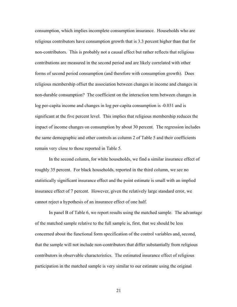
consumption, which implies incomplete consumption insurance. Households who are

religious contributors have consumption growth that is 3.3 percent higher than that for

non-contributors. This is probably not a causal effect but rather reflects that religious

contributions are measured in the second period and are likely correlated with other

forms of second period consumption (and therefore with consumption growth). Does

religious membership offset the association between changes in income and changes in

non-durable consumption? The coefficient on the interaction term between changes in

log per-capita income and changes in log per-capita consumption is -0.031 and is

significant at the five percent level. This implies that religious membership reduces the

impact of income changes on consumption by about 30 percent. The regression includes

the same demographic and other controls as column 2 of Table 5 and their coefficients

remain very close to those reported in Table 5.

In the second column, for white households, we find a similar insurance effect of

roughly 35 percent. For black households, reported in the third column, we see no

statistically significant insurance effect and the point estimate is small with an implied

insurance effect of 7 percent. However, given the relatively large standard error, we

cannot reject a hypothesis of an insurance effect of one half.

In panel B of Table 6, we report results using the matched sample. The advantage

of the matched sample relative to the full sample is, first, that we should be less

concerned about the functional form specification of the control variables and, second,

that the sample will not include non-contributors that differ substantially from religious

contributors in observable characteristics. The estimated insurance effect of religious

participation in the matched sample is very similar to our estimate using the original

21

sample. This reduces our concern that the estimates in the original sample might

somehow be driven by observable differences in demographics between contributors and

non-contributors.

In panel C of Table 6, we present results in which we also add predicted religious

participation (from a probit of religious participation on log household income, the full

set of demographic controls described above, and a full set of year by month dummy

variables) and the interaction of predicted religious participation with the change in log

household income. The results show that the insurance effect is driven entirely by the

orthogonal components of predicted religious membership, i.e., it confirms the

conclusion from panel B that the results are not driven by any observable characteristics

that are correlated with religious participation.

In Table 7, we report the results of a variety of robustness checks on our white

and black samples (we do not report results using the full sample because those results

are almost identical to the results of the white sample). First, in panel A, we re-estimate

our baseline specification measuring income and consumption in per capita terms. For

white households, we see an insurance effect of about 40 percent though this is only

significant at the 10 percent level, while for black households the insurance effect

remains insignificant though the point estimate is now similar to that for whites. Thus,

the results are not very sensitive to whether income changes are measured in per capita

terms or not.

In panel B, we no longer top and bottom code income changes at +/– 100 log

points around the mean income change. When we relax this restriction, the estimated

relationship between changes in income and changes in consumption drops substantially,

22

as would be expected if income changes exceeding +/– 100 log points largely reflect

measurement error or if income is virtually zero in one of the two years. The estimated

insurance effect for whites, however, rises to about 75 percent and remains statistically

significant while the effect for blacks remains insignificant.

In panel C, we define religious membership as equal to 1 if a household

contributes more than $400 (the median contribution, conditional on the contribution

being positive) to religious organizations in a year. For white households, the insurance

effect rises to about 50 percent but is no longer statistically different from zero.

Therefore, our baseline results are driven to a large extent by households that contribute

less than $400 annually to religious organizations – in other words, one does not need to

contribute large sums to religious organizations in order to derive insurance benefits from

them.

In panel D, we use the change in log total consumption expenditure as our

dependent variable instead of using just the non-durable component. Since expenditure

on durable goods results in a consumption flow of durable goods that extends beyond the

quarter in which the expenditure was made, expenditure on durables is a relatively noisy

measure of durable consumption. Thus, someone who ceases to buy durable goods in a

quarter, for example due an income shock, will still generally have the consumption flow

of durables bought in the past. Thus, changes in expenditure on durables can

dramatically overstate changes in the consumption flow from durables. For this reason,

we excluded expenditure on durables in our baseline specification, but the results in panel

D show that we continue to find substantial insurance effects for whites when using total

consumption, though the result is now only significant at the 10 percent level.

23

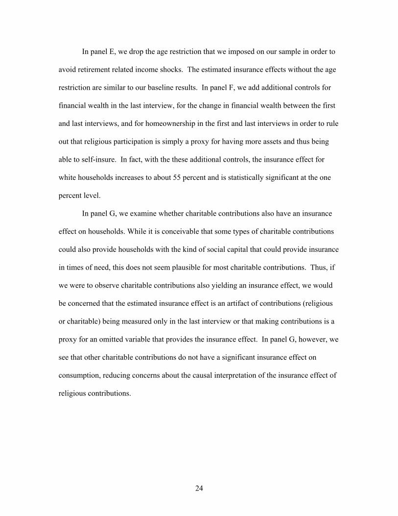
In panel E, we drop the age restriction that we imposed on our sample in order to

avoid retirement related income shocks. The estimated insurance effects without the age

restriction are similar to our baseline results. In panel F, we add additional controls for

financial wealth in the last interview, for the change in financial wealth between the first

and last interviews, and for homeownership in the first and last interviews in order to rule

out that religious participation is simply a proxy for having more assets and thus being

able to self-insure. In fact, with the these additional controls, the insurance effect for

white households increases to about 55 percent and is statistically significant at the one

percent level.

In panel G, we examine whether charitable contributions also have an insurance

effect on households. While it is conceivable that some types of charitable contributions

could also provide households with the kind of social capital that could provide insurance

in times of need, this does not seem plausible for most charitable contributions. Thus, if

we were to observe charitable contributions also yielding an insurance effect, we would

be concerned that the estimated insurance effect is an artifact of contributions (religious

or charitable) being measured only in the last interview or that making contributions is a

proxy for an omitted variable that provides the insurance effect. In panel G, however, we

see that other charitable contributions do not have a significant insurance effect on

consumption, reducing concerns about the causal interpretation of the insurance effect of

religious contributions.

24

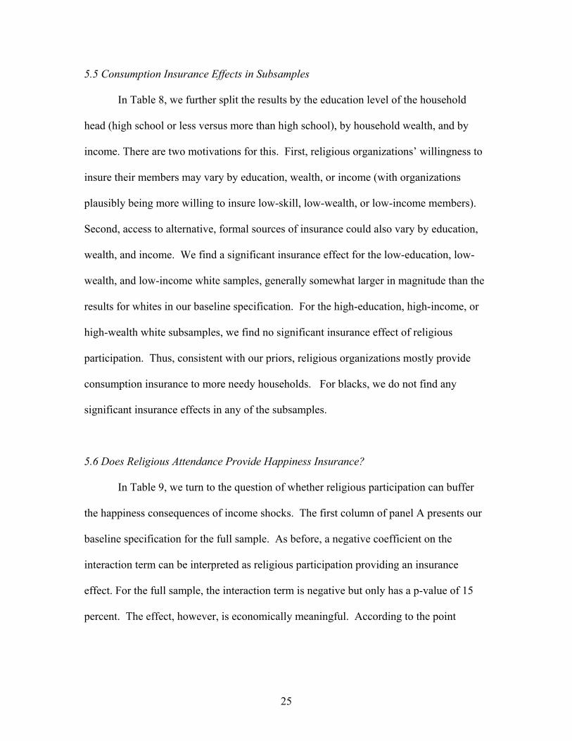
5.5 Consumption Insurance Effects in Subsamples

In Table 8, we further split the results by the education level of the household

head (high school or less versus more than high school), by household wealth, and by

income. There are two motivations for this. First, religious organizations’ willingness to

insure their members may vary by education, wealth, or income (with organizations

plausibly being more willing to insure low-skill, low-wealth, or low-income members).

Second, access to alternative, formal sources of insurance could also vary by education,

wealth, and income. We find a significant insurance effect for the low-education, low-

wealth, and low-income white samples, generally somewhat larger in magnitude than the

results for whites in our baseline specification. For the high-education, high-income, or

high-wealth white subsamples, we find no significant insurance effect of religious

participation. Thus, consistent with our priors, religious organizations mostly provide

consumption insurance to more needy households. For blacks, we do not find any

significant insurance effects in any of the subsamples.

5.6 Does Religious Attendance Provide Happiness Insurance?

In Table 9, we turn to the question of whether religious participation can buffer

the happiness consequences of income shocks. The first column of panel A presents our

baseline specification for the full sample. As before, a negative coefficient on the

interaction term can be interpreted as religious participation providing an insurance

effect. For the full sample, the interaction term is negative but only has a p-value of 15

percent. The effect, however, is economically meaningful. According to the point

25

estimate, the median level of religious participation would buffer about half of the

reduction in happiness from a negative income shock.

In columns (2) and (3), we restrict the samples to whites and to blacks and find

that our results are driven primarily by blacks. For whites, though the results go in the

direction of insurance, the interaction term is not statistically significant, and the point

estimate indicates that the median level religious attendance buffers about 25 percent of

the income shock. For blacks, however, the effect is significant at the five percent level

and is much larger in magnitude. The median level of attendance offsets about 75 percent

of the effect of an income shock on happiness. It is intriguing that our consumption

insurance effects primarily show up for whites while the happiness insurance effects are

strongest for blacks. We discuss and interpret this finding more extensively in Section 6.

Panels B and C of Table 9 explore whether the baseline results could be driven by

differences in observable characteristics between active religious participants and less

active ones. In panel B, we match each individual with above-median religious

attendance to an individual with below-median attendance that has the same predicted

probability of attending above the median, where the prediction is based on same set of

control variables as in our baseline specification. We find that the insurance effects in

our matched sample are very similar to those in our baseline sample, though the estimates

are no longer statistically significant, probably because the sample size is smaller in the

matched sample. In panel C, we interact income shocks both with actual and with

predicted religious attendance. We find that actual rather than predicted religious

attendance drives our baseline results. Thus actual religious attendance, rather than

observable characteristics correlated with attendance, provides the insurance effect.

26

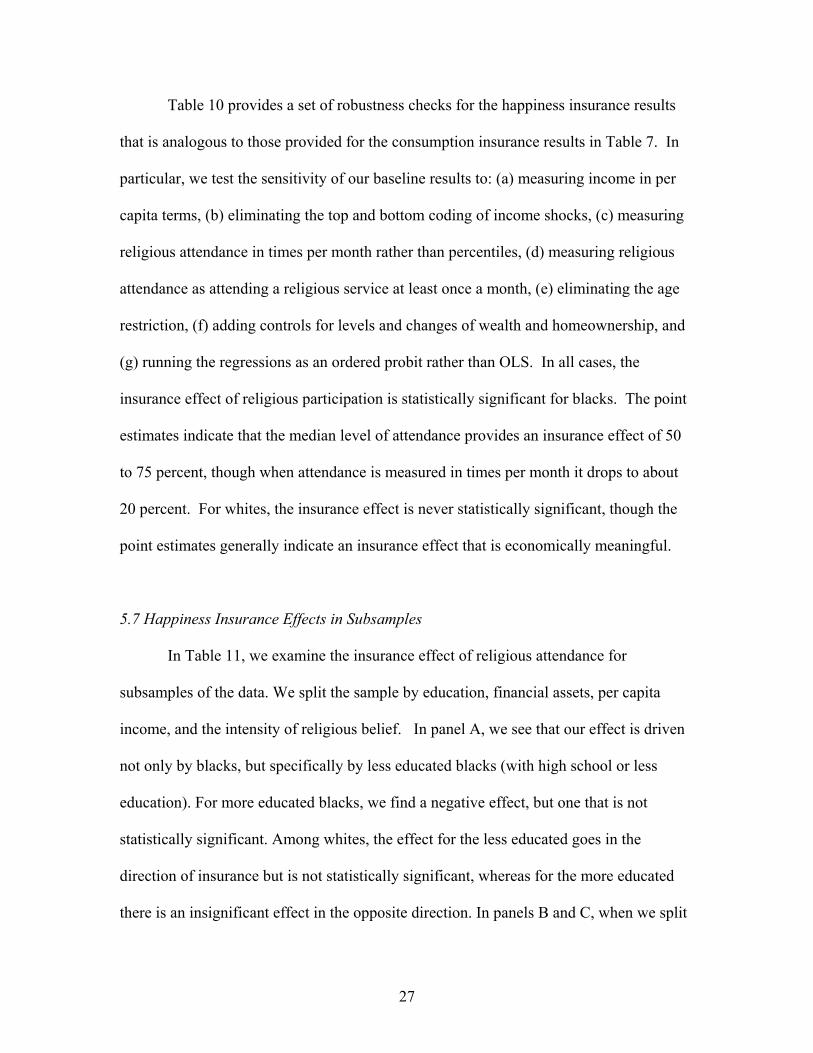
Table 10 provides a set of robustness checks for the happiness insurance results

that is analogous to those provided for the consumption insurance results in Table 7. In

particular, we test the sensitivity of our baseline results to: (a) measuring income in per

capita terms, (b) eliminating the top and bottom coding of income shocks, (c) measuring

religious attendance in times per month rather than percentiles, (d) measuring religious

attendance as attending a religious service at least once a month, (e) eliminating the age

restriction, (f) adding controls for levels and changes of wealth and homeownership, and

(g) running the regressions as an ordered probit rather than OLS. In all cases, the

insurance effect of religious participation is statistically significant for blacks. The point

estimates indicate that the median level of attendance provides an insurance effect of 50

to 75 percent, though when attendance is measured in times per month it drops to about

20 percent. For whites, the insurance effect is never statistically significant, though the

point estimates generally indicate an insurance effect that is economically meaningful.

5.7 Happiness Insurance Effects in Subsamples

In Table 11, we examine the insurance effect of religious attendance for

subsamples of the data. We split the sample by education, financial assets, per capita

income, and the intensity of religious belief. In panel A, we see that our effect is driven

not only by blacks, but specifically by less educated blacks (with high school or less

education). For more educated blacks, we find a negative effect, but one that is not

statistically significant. Among whites, the effect for the less educated goes in the

direction of insurance but is not statistically significant, whereas for the more educated

there is an insignificant effect in the opposite direction. In panels B and C, when we split

27

the data by financial assets and by per capita income, which are presumably closely

correlated with education and each other, we get very similar results. Thus, these

findings echo the earlier consumption insurance results: the insurance effects are

strongest for less educated, lower wealth and lower income individuals, whether it

concerns consumption insurance for whites (Table 8) or happiness insurance for blacks

(Table 11).

Finally, in panel D, we split our results by intensity of religious beliefs as

measured by the average response to two statements about the Bible.10 We find that

those with the greatest intensity of beliefs experience the largest insurance effect; among

blacks this effect is significant and large in magnitude, and among whites this effect

points in the direction of insurance though is not significant. Various mechanisms could

give rise to this finding. Religious organizations could treat all participants equally but

those with more intense beliefs might receive more doctrinal solace from attending after

experiencing a negative income shock. Alternatively, those with more intense beliefs are

more attached to their religious organization (in ways not captured by our measure of

frequency of attending religious service) and the religious organization channels

assistance to more attached members. However, in unreported regressions, we found that

the intensity of beliefs by itself does not provide happiness insurance against income

shocks. Thus, just believing is not sufficient; one needs to participate in a religious

organization to get happiness insurance.

10 Because this question is only relevant for Christians, we drop those reporting a non-Christian religious affiliation from the sample in panel D. The statements are “The Bible is God's word and everything happened or will happen exactly as it says” and “The Bible is the answer to all important human problems” and the response to each statement was recorded on a 5-point scale from “strongly agree” to “strongly disagree.”

28

5.8 Religion versus Alternative Sources of Insurance

It will not be possible for our results to distinguish between the spiritual, social

and material channels though which religious participation may provide happiness

insurance. However, by examining the insurance effect of other social activities, we can

at least determine whether religious organizations play a special role in this regard. These

results are presented in Table 12. In panel A, we interact a range of social activities with

income shocks. For blacks, we find that all social activities go in the direction of

providing insurance for happiness against income shocks, but that only going to social

events at a church, synagogue or mosque is statistically significant. For whites, all

activities go in the direction of insurance (other than going to a bar), but are not

statistically significant.

In panel B, we examine the effect of participating in organizations such as

political and service groups, leisure groups, work-related activities, and religious

organizations. For blacks, the largest effect is from religious organizations, which have a

negative (i.e., insurance) effect, but the coefficient is not statistically significant. For

whites, the largest effect is service or political organizations, and this effect is statistically

significant. This might be an indication that whites have more sources of social capital

than blacks, who rely for a large degree on their religious organizations.

5.9 Insurance Against Other Life Shocks and Effects by Denomination

Table 13 extends our results along two dimensions: we split the results for whites

by religious denomination (the sample size is insufficient to do this for blacks), and we

also examine whether religious participation has an insurance effect for shocks other than

29

income. Using cross-sectional data from the European Social Survey, Clark and Lelkes

(2005) find that the happiness impact of a shock varies crucially by denomination and

type of shock: broadly speaking, church-going Catholics are protected against

unemployment shocks but suffer more if their marriage breaks down, while church-going

protestants are protected against marital shocks but become even more unhappy if

unemployed.

In contrast, we do not find an insurance effect that is significant at the 5 percent

level for any of the 12 regressions by type of shock and religious denomination.

Interestingly though, we find that for Catholics the point estimate for marital shocks is

large, negative and marginally significant. The point estimate for other Christians,

however, is close to zero. Thus, if anything, the evidence points towards an insurance

effect against marital shocks for Catholics. Our results may differ from those from Clark

and Lelkes for a number of reasons such as lack of statistical power of our estimates,

differences between Europe and the United States, the reliance on panel data rather than a

cross-section or the fact that we measure religiosity by the frequency of participation

whereas they measure it by a dummy for the type of religious affiliation.

6. Conclusion

We find that religious participation provides partial insurance against income

shocks but that the mechanism behind this insurance effect appears to differ by race.

Non-durable consumption expenditure of whites who contribute to a religious

organization is about 35 percent less sensitive to income shocks that that of non-

contributing whites. Religious participation, however, does not significantly reduce the

30

happiness impact of income shocks for whites, though the point estimate indicates that

the median level of religious participation reduces the happiness impact of an income

shock by about a quarter. For blacks, however, we do not find significant consumption

insurance effects from religious contributions, though we also cannot reject the

hypothesis that religious participation buffers half of the effect of an income shock on

consumption expenditure. Yet religious organizations do provide significant happiness

insurance for blacks: the median level of religious attendance reduces the happiness

impact of income shocks for blacks by about 75 percent. Moreover, both for whites and

blacks, the insurance effects are strongest for those who seem most vulnerable such as

less educated, low-income, and low-wealth individuals. Our insurance estimates may be

underestimates if religious organizations also provide insurance to those who do not

contribute or to those who are affiliated but do not attend religious services.

The different effects by race might be explained by differences in the ways

religious organizations provide insurance, and the sociological literature provides support

for this explanation. Whites tend to belong to religious organizations where assistance is

more likely to be given in cash11 (and is thus reflected in consumption expenditure), but

where the expectation to repay or the stigma attached to receiving the assistance leads to

little happiness insurance. Assistance in black churches, in contrast, is more likely to be

in the form of social support (thus not reflected in consumption expenditure).

Furthermore, moral or doctrinal support for those experiencing difficulties tends to be

greater in black churches than in white churches, leading to substantial happiness

11 Cnaan (2002), for example, finds that percent white membership of a congregation is a significant and positive predictor of a congregation’s financial commitment to social services, even after controlling for the income and total budget of the congregation.

31

insurance. While these explanations seem plausible, more detailed evidence on the exact

mechanisms by which religious organizations provide insurance remains desirable.

The finding that religious organizations partly insure individuals’ stream of

consumption and of happiness against income shocks has important implications for the

public provision of social insurance. Social insurance is less valuable for those who are

already partly insured through their religious organization, implying that the optimal level

of social insurance is inversely related to the religious participation of the population.

Moreover, social insurance can crowd out insurance provided by religious

organizations.12 Thus, even where Church and State are officially separated,

governments providing less social insurance will indirectly stimulate the demand for

insurance from religious organizations and thus mostly likely strengthen the influence of

religious organizations.

12 Of course, insurance provided by religious organizations may crowd out other forms of private insurance, such as that provided by extended families.

32

33

References

Attanasio, Orazio and Steven J. Davis (1996). “Relative Wage Movements and the Distribution of Consumption.” Journal of Political Economy, 104(6): 1227-1262. Anderson, Gary. M. (1988). “Mr. Smith and the Preachers: The Economics of Religion in the Wealth of Nations.” Journal of Political Economy, 96(5): 1066-1088. Argyle, Michael (1999). “Causes and correlates of happiness.” In Daniel Kahneman, Ed Diener and Norbert Schwarz (eds). Well-Being. The Foundations of Hedonic Psychology. New York, Russell Sage Foundation: 353-373. Azzi, Corry and Ronald G. Ehrenberg (1975). “Household Allocation of Time and Church Attendance.” Journal of Political Economy, 83(1): 27-56.

Barro, Robert J., and Rachel McCleary (2003). “Religion and Economic Growth.” NBER Working Paper No. 9682.

Berman, Eli (2000). “Sect, Subsidy, and Sacrifice: An Economist's View of Ultra-orthodox Jews.” Quarterly Journal of Economics, 115(3): 905-953.

Biddle, Jeff E. (1992). “Religious Organizations.” In Charles T. Clotfelter (ed.), Who Benefits From the Non-Profit Sector? Chicago: University of Chicago. Blanchflower, David G. and Andrew J. Oswald (2004). “Well-Being over Time in Britain and the USA,” Journal of Public Economics, 88(7-8): 1359-1386. Carson, Emmett (1990), “Patterns of Giving in Black Churches.” In Robert Wuthnow and Virginia Hodgkinson (eds.), Faith and Philanthropy in America: Exploring the Role of Religion in America’s Voluntary Sector. San Francisco: Jossey-Bass Publishers: 232-252. Chaves, Mark (2004). Congregations in America. Cambridge, MA: Harvard University Press. Chaves, Mark, and Lynn Higgins (1992), “Comparing the Community Involvement of Black and White Congregations,” Journal for the Scientific Study of Religion, Volume 31 (4): 425-440. Chen, Daniel (2004). “Club Goods and Group Identity: Evidence from the Islamic Resurgence During the Indonesian Financial Crisis.” manuscript, University of Chicago. Clark, Andrew and Orsolya Lelkes (2005) “Deliver us from Evil: Religion as Insurance.” manuscript, PSE, Paris. Cnaan, Ram (2002). The Invisible Caring Hand: American Congregations and the Provision of Welfare. New York: New York University Press.

34

Cochrane, John A. (1991). “A Simple Test of Consumption Insurance” Journal of Political Economy, 99(5): 957-976. Deaton, Angus (1992). “Household Saving in LDCs: Credit Markets, Insurance, and Welfare.” Scandinavian Journal of Economics, 94(2): 253-273. Diener, Ed and Robert Biswas-Diener (2002). “Will Money Increase Subjective Well-Being?” Social Indicators Research, 57: 119-169. Diener, Ed, Eunkook M. Suh, Richard E. Lucas, and Heidi L. Smith (1999). “Subjective Well-being: Three Decades of Progress.” Psychological Bulletin, 125(2): 276-303. Di Tella, Rafael, John Haisken-De New, and Robert MacCulloch (2005), “Adaptation to Income and Status in an Individual Panel.” Manuscript, Harvard University. Ellison, Christopher G. (1991). “Religious Involvement and Subjective Well-Being.” Journal of Health and Social Behavior, 32(1): 80-99. Foster, Andrew and Mark Rosenzweig (2001). “Imperfect Commitment, Altruism, and the Family: Evidence from Transfer Behavior in Low-Income Rural Areas.” Review of Economics and Statistics, 83(3): 389-407. Freeman, Richard B. (1986). “Who Escapes? The Relation of Churchgoing and other Background Factors to the Socioeconomic Performance of Black Male Youths from Inner-city Tracts.” In Richard B. Freeman and Harry J. Holzer (eds.), The Black Youth Employment Crisis. Chicago, University of Chicago Press: 353-376. Frey, Bruno S. and Alois Stutzer. 2002. “What Can Economists Learn from Happiness Research?” Journal of Economic Literature, 40(2): 402-35. Genicot, Garance, and Debraj Ray (2003). “Group Formation in Risk-Sharing Agreements.” Review of Economic Studies, 70(1): 87-113. Gertler, Paul and Jonathan Gruber (2002). “Insuring Consumption Against Illness.” American Economic Review, 92: 51–70. Guiso, Luigi, Paola Sapienza, and Luigi Zingales (2004). “The Role of Social Capital in Financial Development.” American Economic Review, 94(3): 526-556. Gruber, Jonathan (2004). “Pay or Pray? The Impact of Charitable Subsidies on Religious Attendance.” Journal of Public Economics, 88(12): 2635-2655. Gruber, Jonathan (2005). “Religious Market Structure, Religious Participation, and Outcomes: Is Religion Good for You?” NBER working paper No. 11377.

35

Gruber, Jonathan and Daniel M. Hungerman (2005). “Faith-Based Charity and Crowd Out during the Great Depression.” NBER working paper No. 11332. Gruber, Jonathan and Sendhil Mullainathan (2005). “Do Cigarette Taxes Make Smokers Happier?” The B.E. Journals in Economic Analysis & Policy, forthcoming. Hungerman, Daniel M. (2005). “Are Church and State Substitutes? Evidence from the 1996 Welfare Reform.” Journal of Public Economics, forthcoming. Iannaccone, Laurence R. (1990). “Religious Participation: A Human Capital Approach.” Journal for the Scientific Study of Religion, 29(3): 297-314. Iannaccone, Laurence R. (1992). “Sacrifice and Stigma: Reducing Free-riding in Cults, Communes, and Other Collectives.” Journal of Political Economy, 100(2): 271-291. Iannaccone, Laurence R. (1998). “Introduction to the Economics of Religion.” Journal of Economic Literature, 36(3): 1465-1495. MacCulloch, Robert and Silvia Pezzini (2004). “The Role of Freedom, Growth and Religion in the Taste for Revolution.” Manuscript, Imperial College London.

Mace, Barbara J. (1991). “Full Insurance in the Presence of Aggregate Uncertainty.” Journal of Political Economy, 99(5): 928-56.

McCullough, Michael E., William T. Hoyt, David B. Larson, Harold G. Koenig, and Carl Thoresen (2000). “Religious Involvement and Mortality: A Meta-Analytic Review.” Health Psychology, 19(3): 211-222.

Nelson, Julie A. (1994). “On Testing for Full Insurance using Consumer Expenditure Survey Data.” Journal of Political Economy, 102(2): 384-394. Pargament, Kenneth I. (2002). “The Bitter and the Sweet: An Evaluation of the Costs and Benefits of Religiousness.” Psychological Inquiry, 13(3): 168-181. Putman, Robert D. (2000). Bowling Along: The Collapse and Revival of American Community. New York: Simon & Schuster. Stasavage, David, and Ken Scheve (2005). “Religion and Preferences for Social Insurance.” Manuscript, London School of Economics. Strawbridge, William J., Sarah J. Shema, Richard D. Cohen, Robert E. Roberts, and George A. Kaplan (1998). “Religiosity Buffers Effects of Some Stressors on Depression but Exacerbates Others.” Journals of Gerontology, 53B(3): 118-126.

36

Smith, Timothy B., Michael E. McCullough, and Justin Poll (2003). “Religiousness and Depression: Evidence for a Main Effect and the Moderating Influence of Stressful Life Events.” Psychological Bulletin, 129(4): 614-636. Sweet, James A., and Larry L. Bumpass (1996). “The National Survey of Families and Households - Waves 1 and 2: Data Description and Documentation,” Center for Demography and Ecology, University of Wisconsin-Madison (http://www.ssc.wisc.edu/nsfh/home.htm). Sweet, James A., Larry L. Bumpass, and Vaughn Call (1988). “The Design and Content of The National Survey of Families and Households,” Center for Demography and Ecology, University of Wisconsin-Madison, NSFH Working Paper No. 1. Townsend, Robert M. (1994). “Risk and Insurance in Village India.” Econometrica, 62(3): 539-591.

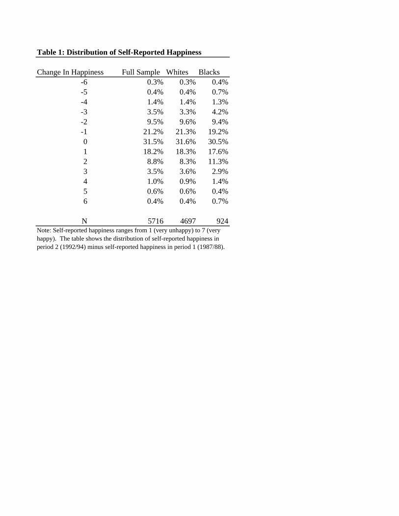
Table 1: Distribution of Self-Reported Happiness

Change In Happiness Full Sample Whites Blacks-6 0.3% 0.3% 0.4%-5 0.4% 0.4% 0.7%-4 1.4% 1.4% 1.3%-3 3.5% 3.3% 4.2%-2 9.5% 9.6% 9.4%-1 21.2% 21.3% 19.2%0 31.5% 31.6% 30.5%1 18.2% 18.3% 17.6%2 8.8% 8.3% 11.3%3 3.5% 3.6% 2.9%4 1.0% 0.9% 1.4%5 0.6% 0.6% 0.4%6 0.4% 0.4% 0.7%

N 5716 4697 924Note: Self-reported happiness ranges from 1 (very unhappy) to 7 (very happy). The table shows the distribution of self-reported happiness in period 2 (1992/94) minus self-reported happiness in period 1 (1987/88).

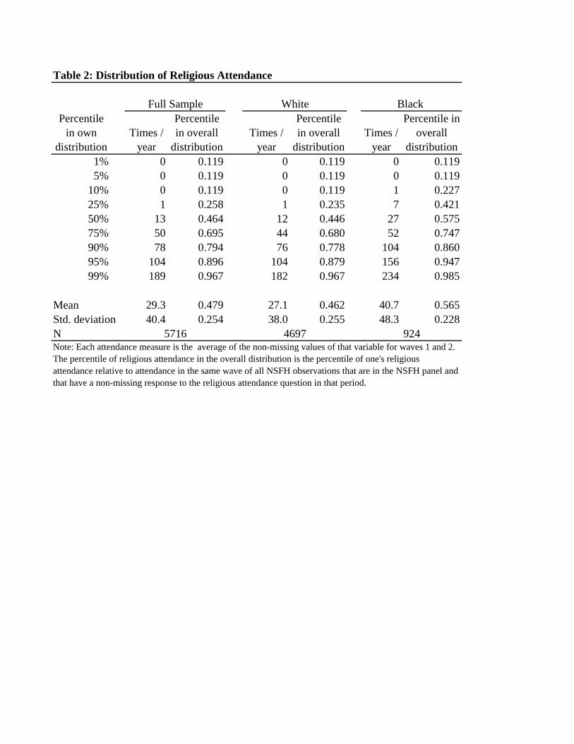
Table 2: Distribution of Religious Attendance

Percentile in own

distributionTimes /

year

Percentile in overall

distributionTimes /

year

Percentile in overall

distributionTimes /

year

Percentile in overall

distribution1% 0 0.119 0 0.119 0 0.1195% 0 0.119 0 0.119 0 0.119

10% 0 0.119 0 0.119 1 0.22725% 1 0.258 1 0.235 7 0.42150% 13 0.464 12 0.446 27 0.57575% 50 0.695 44 0.680 52 0.74790% 78 0.794 76 0.778 104 0.86095% 104 0.896 104 0.879 156 0.94799% 189 0.967 182 0.967 234 0.985

Mean 29.3 0.479 27.1 0.462 40.7 0.565Std. deviation 40.4 0.254 38.0 0.255 48.3 0.228N

Full Sample White Black

Note: Each attendance measure is the average of the non-missing values of that variable for waves 1 and 2. The percentile of religious attendance in the overall distribution is the percentile of one's religious attendance relative to attendance in the same wave of all NSFH observations that are in the NSFH panel and that have a non-missing response to the religious attendance question in that period.

5716 4697 924

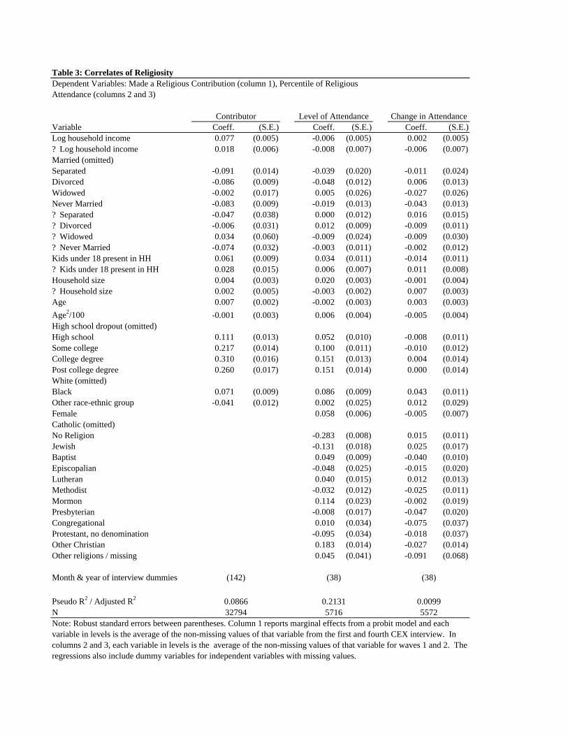
Table 3: Correlates of Religiosity

Variable Coeff. (S.E.) Coeff. (S.E.) Coeff. (S.E.)Log household income 0.077 (0.005) -0.006 (0.005) 0.002 (0.005)? Log household income 0.018 (0.006) -0.008 (0.007) -0.006 (0.007)Married (omitted)Separated -0.091 (0.014) -0.039 (0.020) -0.011 (0.024)Divorced -0.086 (0.009) -0.048 (0.012) 0.006 (0.013)Widowed -0.002 (0.017) 0.005 (0.026) -0.027 (0.026)Never Married -0.083 (0.009) -0.019 (0.013) -0.043 (0.013)? Separated -0.047 (0.038) 0.000 (0.012) 0.016 (0.015)? Divorced -0.006 (0.031) 0.012 (0.009) -0.009 (0.011)? Widowed 0.034 (0.060) -0.009 (0.024) -0.009 (0.030)? Never Married -0.074 (0.032) -0.003 (0.011) -0.002 (0.012)Kids under 18 present in HH 0.061 (0.009) 0.034 (0.011) -0.014 (0.011)? Kids under 18 present in HH 0.028 (0.015) 0.006 (0.007) 0.011 (0.008)Household size 0.004 (0.003) 0.020 (0.003) -0.001 (0.004)? Household size 0.002 (0.005) -0.003 (0.002) 0.007 (0.003)Age 0.007 (0.002) -0.002 (0.003) 0.003 (0.003)Age2/100 -0.001 (0.003) 0.006 (0.004) -0.005 (0.004)High school dropout (omitted)High school 0.111 (0.013) 0.052 (0.010) -0.008 (0.011)Some college 0.217 (0.014) 0.100 (0.011) -0.010 (0.012)College degree 0.310 (0.016) 0.151 (0.013) 0.004 (0.014)Post college degree 0.260 (0.017) 0.151 (0.014) 0.000 (0.014)White (omitted)Black 0.071 (0.009) 0.086 (0.009) 0.043 (0.011)Other race-ethnic group -0.041 (0.012) 0.002 (0.025) 0.012 (0.029)Female 0.058 (0.006) -0.005 (0.007)Catholic (omitted)No Religion -0.283 (0.008) 0.015 (0.011)Jewish -0.131 (0.018) 0.025 (0.017)Baptist 0.049 (0.009) -0.040 (0.010)Episcopalian -0.048 (0.025) -0.015 (0.020)Lutheran 0.040 (0.015) 0.012 (0.013)Methodist -0.032 (0.012) -0.025 (0.011)Mormon 0.114 (0.023) -0.002 (0.019)Presbyterian -0.008 (0.017) -0.047 (0.020)Congregational 0.010 (0.034) -0.075 (0.037)Protestant, no denomination -0.095 (0.034) -0.018 (0.037)Other Christian 0.183 (0.014) -0.027 (0.014)Other religions / missing 0.045 (0.041) -0.091 (0.068)

Month & year of interview dummies

Pseudo R2 / Adjusted R2

N

Dependent Variables: Made a Religious Contribution (column 1), Percentile of Religious Attendance (columns 2 and 3)

0.086632794

0.21315716

Level of Attendance Change in AttendanceContributor

Note: Robust standard errors between parentheses. Column 1 reports marginal effects from a probit model and each variable in levels is the average of the non-missing values of that variable from the first and fourth CEX interview. In columns 2 and 3, each variable in levels is the average of the non-missing values of that variable for waves 1 and 2. The regressions also include dummy variables for independent variables with missing values.

0.00995572

(142) (38) (38)

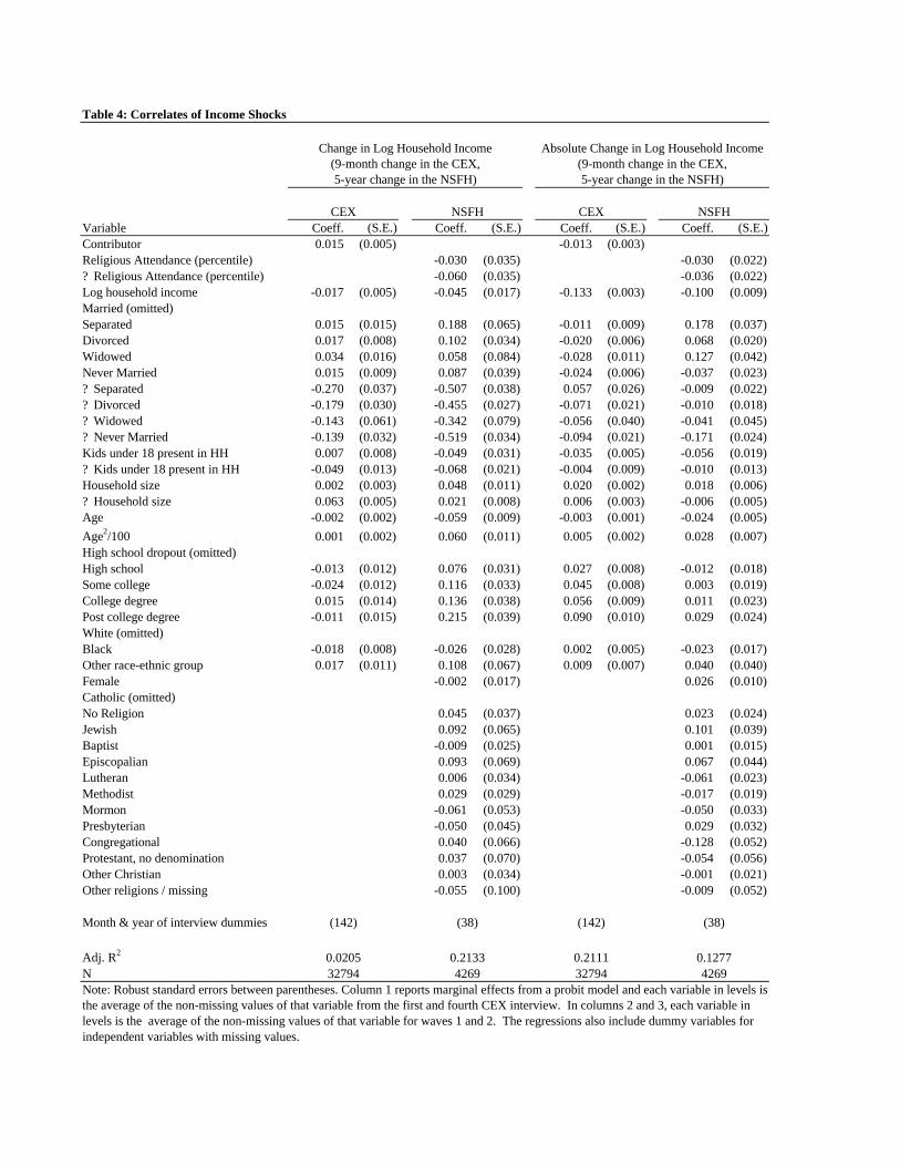
Table 4: Correlates of Income Shocks

Variable Coeff. (S.E.) Coeff. (S.E.) Coeff. (S.E.) Coeff. (S.E.)Contributor 0.015 (0.005) -0.013 (0.003)Religious Attendance (percentile) -0.030 (0.035) -0.030 (0.022)? Religious Attendance (percentile) -0.060 (0.035) -0.036 (0.022)Log household income -0.017 (0.005) -0.045 (0.017) -0.133 (0.003) -0.100 (0.009)Married (omitted)Separated 0.015 (0.015) 0.188 (0.065) -0.011 (0.009) 0.178 (0.037)Divorced 0.017 (0.008) 0.102 (0.034) -0.020 (0.006) 0.068 (0.020)Widowed 0.034 (0.016) 0.058 (0.084) -0.028 (0.011) 0.127 (0.042)Never Married 0.015 (0.009) 0.087 (0.039) -0.024 (0.006) -0.037 (0.023)? Separated -0.270 (0.037) -0.507 (0.038) 0.057 (0.026) -0.009 (0.022)? Divorced -0.179 (0.030) -0.455 (0.027) -0.071 (0.021) -0.010 (0.018)? Widowed -0.143 (0.061) -0.342 (0.079) -0.056 (0.040) -0.041 (0.045)? Never Married -0.139 (0.032) -0.519 (0.034) -0.094 (0.021) -0.171 (0.024)Kids under 18 present in HH 0.007 (0.008) -0.049 (0.031) -0.035 (0.005) -0.056 (0.019)? Kids under 18 present in HH -0.049 (0.013) -0.068 (0.021) -0.004 (0.009) -0.010 (0.013)Household size 0.002 (0.003) 0.048 (0.011) 0.020 (0.002) 0.018 (0.006)? Household size 0.063 (0.005) 0.021 (0.008) 0.006 (0.003) -0.006 (0.005)Age -0.002 (0.002) -0.059 (0.009) -0.003 (0.001) -0.024 (0.005)Age2/100 0.001 (0.002) 0.060 (0.011) 0.005 (0.002) 0.028 (0.007)High school dropout (omitted)High school -0.013 (0.012) 0.076 (0.031) 0.027 (0.008) -0.012 (0.018)Some college -0.024 (0.012) 0.116 (0.033) 0.045 (0.008) 0.003 (0.019)College degree 0.015 (0.014) 0.136 (0.038) 0.056 (0.009) 0.011 (0.023)Post college degree -0.011 (0.015) 0.215 (0.039) 0.090 (0.010) 0.029 (0.024)White (omitted)Black -0.018 (0.008) -0.026 (0.028) 0.002 (0.005) -0.023 (0.017)Other race-ethnic group 0.017 (0.011) 0.108 (0.067) 0.009 (0.007) 0.040 (0.040)Female -0.002 (0.017) 0.026 (0.010)Catholic (omitted)No Religion 0.045 (0.037) 0.023 (0.024)Jewish 0.092 (0.065) 0.101 (0.039)Baptist -0.009 (0.025) 0.001 (0.015)Episcopalian 0.093 (0.069) 0.067 (0.044)Lutheran 0.006 (0.034) -0.061 (0.023)Methodist 0.029 (0.029) -0.017 (0.019)Mormon -0.061 (0.053) -0.050 (0.033)Presbyterian -0.050 (0.045) 0.029 (0.032)Congregational 0.040 (0.066) -0.128 (0.052)Protestant, no denomination 0.037 (0.070) -0.054 (0.056)Other Christian 0.003 (0.034) -0.001 (0.021)Other religions / missing -0.055 (0.100) -0.009 (0.052)

Month & year of interview dummies

Adj. R2

N 32794Note: Robust standard errors between parentheses. Column 1 reports marginal effects from a probit model and each variable in levels is the average of the non-missing values of that variable from the first and fourth CEX interview. In columns 2 and 3, each variable in levels is the average of the non-missing values of that variable for waves 1 and 2. The regressions also include dummy variables for independent variables with missing values.

NSFHCEX

42690.21334269 32794

(38)

Change in Log Household Income (9-month change in the CEX, 5-year change in the NSFH)

Absolute Change in Log Household Income (9-month change in the CEX, 5-year change in the NSFH)

0.0205

(142)

CEX NSFH

0.2111

(142) (38)

0.1277

Table 5: Correlates of Consumption and Self-Reported HappinessDependent Variable: Log Quarterly Household Non-Durable Expenditure / Self-Reported Happiness

Variable Coeff. (S.E.) Coeff. (S.E.) Coeff. (S.E.) Coeff. (S.E.)Contributor 0.082 (0.007) 0.032 (0.009)Religious Attendance (percentile) 0.526 (0.060) -0.067 (0.095)? Religious Attendance (percentile) 0.149 (0.095)Log household income 0.366 (0.007) -0.006 (0.006) 0.175 (0.023) -0.054 (0.037)? Log household income 0.020 (0.008) 0.084 (0.010) 0.153 (0.050)Married (omitted)Separated -0.146 (0.018) -0.002 (0.023) -0.677 (0.102) 0.065 (0.166)Divorced -0.130 (0.011) -0.010 (0.014) -0.393 (0.056) 0.169 (0.089)Widowed -0.154 (0.021) 0.021 (0.025) -0.717 (0.126) 0.262 (0.202)Never Married -0.195 (0.012) 0.000 (0.015) -0.322 (0.058) 0.085 (0.092)? Separated -0.112 (0.060) -0.797 (0.105)? Divorced -0.145 (0.052) -0.279 (0.079)? Widowed -0.259 (0.098) -0.677 (0.187)? Never Married -0.200 (0.054) -0.421 (0.084)Kids under 18 present in HH -0.143 (0.010) 0.043 (0.013) -0.065 (0.050) -0.092 (0.078)? Kids under 18 present in HH -0.028 (0.022) -0.056 (0.053)Household size 0.109 (0.003) -0.006 (0.004) -0.026 (0.015) 0.015 (0.025)? Household size 0.091 (0.008) -0.011 (0.018)Age 0.022 (0.003) 0.003 (0.003) -0.050 (0.014) 0.005 (0.022)Age2/100 -0.024 (0.003) -0.003 (0.004) 0.056 (0.018) 0.002 (0.028)High school dropout (omitted)High school 0.142 (0.015) 0.012 (0.019) -0.021 (0.052) -0.029 (0.080)Some college 0.280 (0.016) 0.021 (0.020) 0.024 (0.055) 0.052 (0.085)College degree 0.359 (0.019) 0.023 (0.023) 0.013 (0.063) 0.013 (0.099)Post college degree 0.455 (0.021) 0.026 (0.025) -0.012 (0.065) -0.143 (0.103)White (omitted)Black -0.183 (0.010) -0.033 (0.013) 0.049 (0.045) -0.021 (0.070)Other race-ethnic group -0.105 (0.015) -0.003 (0.019) -0.086 (0.108) -0.222 (0.146)Female 0.003 (0.028) -0.024 (0.045)Catholic (omitted)No Religion -0.056 (0.063) 0.029 (0.097)Jewish -0.087 (0.100) 0.024 (0.165)Baptist 0.014 (0.041) 0.022 (0.067)Episcopalian 0.017 (0.107) 0.067 (0.154)Lutheran 0.008 (0.061) 0.021 (0.086)Methodist 0.047 (0.052) -0.026 (0.077)Mormon -0.113 (0.099) -0.069 (0.150)Presbyterian 0.020 (0.082) -0.015 (0.127)Congregational -0.121 (0.140) -0.018 (0.279)Protestant, no denomination 0.055 (0.151) 0.231 (0.214)Other Christian 0.001 (0.059) -0.052 (0.088)Other religions / missing -0.282 (0.208) 0.416 (0.206)

Month & year of interview dummies

Adj. R2

N

(38)

57163279432794

(142) (142) (38)

Level of Happiness

Change in Happiness

Note: Robust standard errors between parentheses. Column 1 reports marginal effects from a probit model and each variable in levels is the average of the non-missing values of that variable from the first and fourth CEX interview. In columns 2 and 3, each variable in levels is the average of the non-missing values of that variable for waves 1 and 2. The regressions also include dummy variables for independent variables with missing values.

Level of Consumption

Change in Consumption

0.3957 0.0311 0.0808 0.02795716

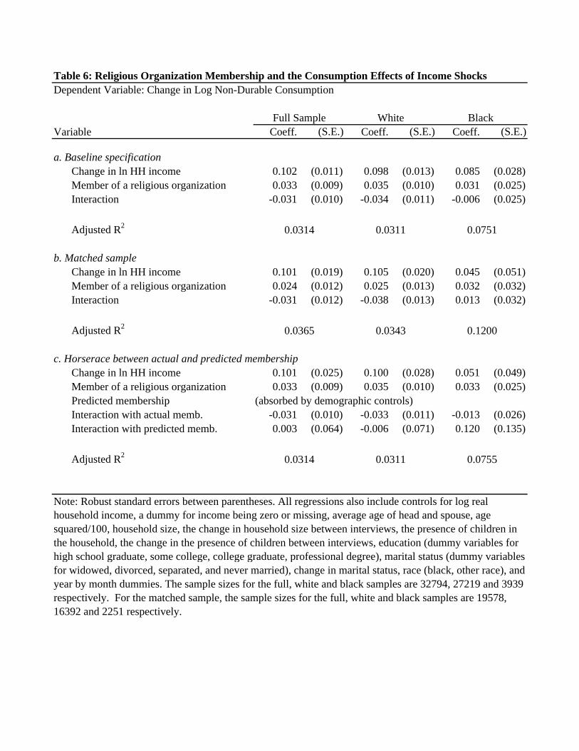
Table 6: Religious Organization Membership and the Consumption Effects of Income ShocksDependent Variable: Change in Log Non-Durable Consumption

Variable Coeff. (S.E.) Coeff. (S.E.) Coeff. (S.E.)

a. Baseline specificationChange in ln HH income 0.102 (0.011) 0.098 (0.013) 0.085 (0.028)Member of a religious organization 0.033 (0.009) 0.035 (0.010) 0.031 (0.025)Interaction -0.031 (0.010) -0.034 (0.011) -0.006 (0.025)

Adjusted R2

b. Matched sampleChange in ln HH income 0.101 (0.019) 0.105 (0.020) 0.045 (0.051)Member of a religious organization 0.024 (0.012) 0.025 (0.013) 0.032 (0.032)Interaction -0.031 (0.012) -0.038 (0.013) 0.013 (0.032)

Adjusted R2

c. Horserace between actual and predicted membershipChange in ln HH income 0.101 (0.025) 0.100 (0.028) 0.051 (0.049)Member of a religious organization 0.033 (0.009) 0.035 (0.010) 0.033 (0.025)Predicted membership (absorbed by demographic controls)Interaction with actual memb. -0.031 (0.010) -0.033 (0.011) -0.013 (0.026)Interaction with predicted memb. 0.003 (0.064) -0.006 (0.071) 0.120 (0.135)

Adjusted R2

0.1200

0.0314 0.0311 0.0755

Full Sample White Black

Note: Robust standard errors between parentheses. All regressions also include controls for log real household income, a dummy for income being zero or missing, average age of head and spouse, age squared/100, household size, the change in household size between interviews, the presence of children in the household, the change in the presence of children between interviews, education (dummy variables for high school graduate, some college, college graduate, professional degree), marital status (dummy variables for widowed, divorced, separated, and never married), change in marital status, race (black, other race), and year by month dummies. The sample sizes for the full, white and black samples are 32794, 27219 and 3939 respectively. For the matched sample, the sample sizes for the full, white and black samples are 19578, 16392 and 2251 respectively.

0.0314 0.0311 0.0751

0.0365 0.0343

Table 7: Robustness Checks: Religious Organization Membership and Consumption

Variable Coeff. (S.E.) Coeff. (S.E.)

a. Income measured in per capita termsChange in ln HH income p.c. 0.095 (0.013) 0.101 (0.029)Member of a religious organization 0.033 (0.010) 0.027 (0.025)Interaction -0.040 (0.022) -0.033 (0.053)Adjusted R2

b. Shocks not top and bottom coded at 100 log point difference from mean shockChange in ln HH income 0.034 (0.007) 0.038 (0.017)Member of a religious organization 0.035 (0.010) 0.030 (0.025)Interaction -0.027 (0.012) -0.007 (0.028)Adjusted R2

c. Membership measured as above median contribution ($400)Change in ln HH income 0.183 (0.121) -0.219 (0.181)Member of a religious organization 0.001 (0.054) 0.113 (0.095)Interaction -0.094 (0.122) 0.317 (0.183)Adjusted R2

d. Change in log total consumption expenditure used as dependent variableChange in ln HH income 0.072 (0.010) 0.064 (0.021)Member of a religious organization 0.032 (0.007) 0.034 (0.019)Interaction -0.030 (0.017) 0.006 (0.040)Adjusted R2

e. No age restriction on the sampleChange in ln HH income 0.116 (0.011) 0.088 (0.026)Member of a religious organization 0.035 (0.008) 0.018 (0.021)Interaction -0.065 (0.018) 0.017 (0.044)Adjusted R2

f. Additional controls for wealth and homeownershipChange in ln HH income 0.096 (0.014) 0.089 (0.029)Member of a religious organization 0.035 (0.010) 0.032Interaction -0.050 (0.023) -0.022 (0.055)Adjusted R2

g. Horserace between charitable contributions and church membershipChange in ln HH income 0.121 (0.012) 0.089 (0.026)Church membership 0.032 (0.008) 0.010 (0.022)Made charitable contribution 0.014 (0.009) 0.041 (0.027)Interaction with church membership -0.058 (0.019) 0.022 (0.047)Interaction with charitable contribution -0.023 (0.020) -0.026 (0.060)Adjusted R2

White Black

0.0862

0.0304 0.0709

0.0400 0.0854

0.0326

Note: Robust standard errors between parentheses. All regressions also include the controls from the baseline regression (table 6, panel a). The sample sizes for the white and black sample are 27219 and 3939 respectively.

0.0481 0.1052

0.0297 0.0741

0.0311 0.0753

0.0305 0.0713

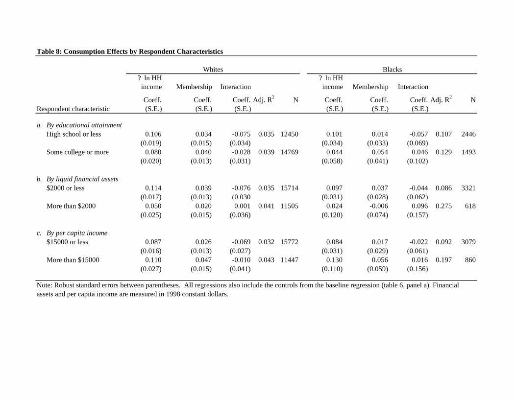
Table 8: Consumption Effects by Respondent Characteristics

? ln HH income Membership Interaction

? ln HH income Membership Interaction

Coeff. Coeff. Coeff. Adj. R2 N Coeff. Coeff. Coeff. Adj. R2 NRespondent characteristic (S.E.) (S.E.) (S.E.) (S.E.) (S.E.) (S.E.)

a. By educational attainmentHigh school or less 0.106 0.034 -0.075 0.035 12450 0.101 0.014 -0.057 0.107 2446

(0.019) (0.015) (0.034) (0.034) (0.033) (0.069)Some college or more 0.080 0.040 -0.028 0.039 14769 0.044 0.054 0.046 0.129 1493

(0.020) (0.013) (0.031) (0.058) (0.041) (0.102)

b. By liquid financial assets$2000 or less 0.114 0.039 -0.076 0.035 15714 0.097 0.037 -0.044 0.086 3321

(0.017) (0.013) (0.030 (0.031) (0.028) (0.062)More than $2000 0.050 0.020 0.001 0.041 11505 0.024 -0.006 0.096 0.275 618

(0.025) (0.015) (0.036) (0.120) (0.074) (0.157)

c. By per capita income$15000 or less 0.087 0.026 -0.069 0.032 15772 0.084 0.017 -0.022 0.092 3079

(0.016) (0.013) (0.027) (0.031) (0.029) (0.061)More than $15000 0.110 0.047 -0.010 0.043 11447 0.130 0.056 0.016 0.197 860

(0.027) (0.015) (0.041) (0.110) (0.059) (0.156)

Blacks

Note: Robust standard errors between parentheses. All regressions also include the controls from the baseline regression (table 6, panel a). Financial assets and per capita income are measured in 1998 constant dollars.

Whites

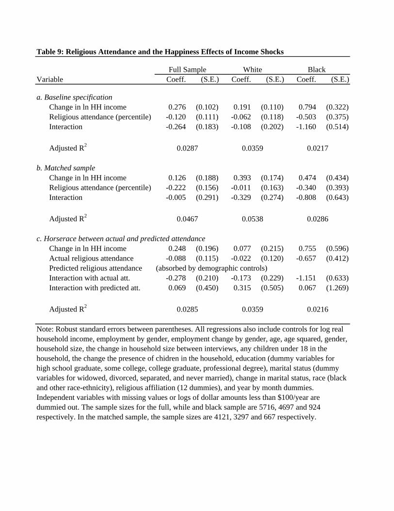
Table 9: Religious Attendance and the Happiness Effects of Income Shocks

Variable Coeff. (S.E.) Coeff. (S.E.) Coeff. (S.E.)

a. Baseline specificationChange in ln HH income 0.276 (0.102) 0.191 (0.110) 0.794 (0.322)Religious attendance (percentile) -0.120 (0.111) -0.062 (0.118) -0.503 (0.375)Interaction -0.264 (0.183) -0.108 (0.202) -1.160 (0.514)

Adjusted R2

b. Matched sampleChange in ln HH income 0.126 (0.188) 0.393 (0.174) 0.474 (0.434)Religious attendance (percentile) -0.222 (0.156) -0.011 (0.163) -0.340 (0.393)Interaction -0.005 (0.291) -0.329 (0.274) -0.808 (0.643)

Adjusted R2

c. Horserace between actual and predicted attendanceChange in ln HH income 0.248 (0.196) 0.077 (0.215) 0.755 (0.596)Actual religious attendance -0.088 (0.115) -0.022 (0.120) -0.657 (0.412)Predicted religious attendance (absorbed by demographic controls)Interaction with actual att. -0.278 (0.210) -0.173 (0.229) -1.151 (0.633)Interaction with predicted att. 0.069 (0.450) 0.315 (0.505) 0.067 (1.269)

Adjusted R2

Full Sample White Black

Note: Robust standard errors between parentheses. All regressions also include controls for log real household income, employment by gender, employment change by gender, age, age squared, gender, household size, the change in household size between interviews, any children under 18 in the household, the change the presence of chidren in the household, education (dummy variables for high school graduate, some college, college graduate, professional degree), marital status (dummy variables for widowed, divorced, separated, and never married), change in marital status, race (black and other race-ethnicity), religious affiliation (12 dummies), and year by month dummies. Independent variables with missing values or logs of dollar amounts less than $100/year are dummied out. The sample sizes for the full, while and black sample are 5716, 4697 and 924 respectively. In the matched sample, the sample sizes are 4121, 3297 and 667 respectively.

0.0287 0.0359 0.0217

0.0467 0.0538 0.0286

0.0285 0.0359 0.0216

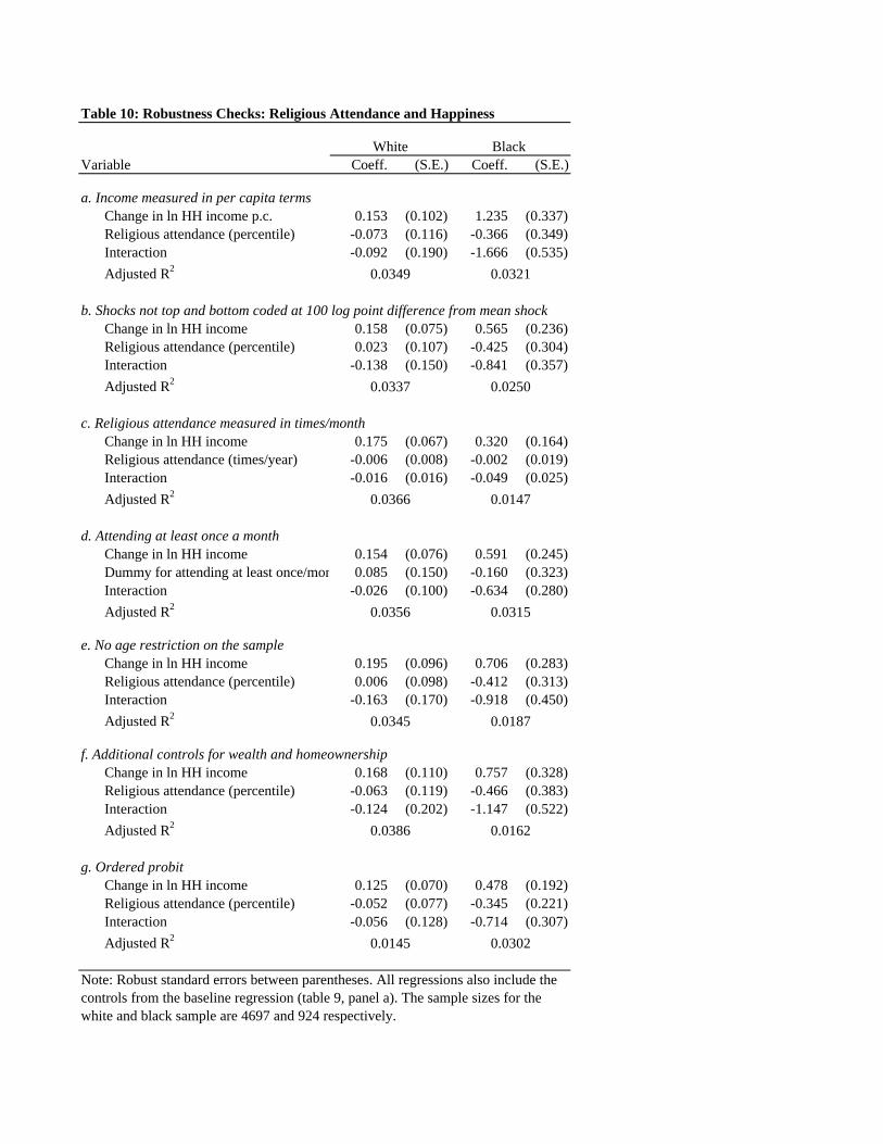
Table 10: Robustness Checks: Religious Attendance and Happiness

Variable Coeff. (S.E.) Coeff. (S.E.)

a. Income measured in per capita termsChange in ln HH income p.c. 0.153 (0.102) 1.235 (0.337)Religious attendance (percentile) -0.073 (0.116) -0.366 (0.349)Interaction -0.092 (0.190) -1.666 (0.535)Adjusted R2

b. Shocks not top and bottom coded at 100 log point difference from mean shockChange in ln HH income 0.158 (0.075) 0.565 (0.236)Religious attendance (percentile) 0.023 (0.107) -0.425 (0.304)Interaction -0.138 (0.150) -0.841 (0.357)Adjusted R2

c. Religious attendance measured in times/monthChange in ln HH income 0.175 (0.067) 0.320 (0.164)Religious attendance (times/year) -0.006 (0.008) -0.002 (0.019)Interaction -0.016 (0.016) -0.049 (0.025)Adjusted R2

d. Attending at least once a monthChange in ln HH income 0.154 (0.076) 0.591 (0.245)Dummy for attending at least once/month 0.085 (0.150) -0.160 (0.323)Interaction -0.026 (0.100) -0.634 (0.280)Adjusted R2

e. No age restriction on the sampleChange in ln HH income 0.195 (0.096) 0.706 (0.283)Religious attendance (percentile) 0.006 (0.098) -0.412 (0.313)Interaction -0.163 (0.170) -0.918 (0.450)Adjusted R2

f. Additional controls for wealth and homeownershipChange in ln HH income 0.168 (0.110) 0.757 (0.328)Religious attendance (percentile) -0.063 (0.119) -0.466 (0.383)Interaction -0.124 (0.202) -1.147 (0.522)Adjusted R2

g. Ordered probitChange in ln HH income 0.125 (0.070) 0.478 (0.192)Religious attendance (percentile) -0.052 (0.077) -0.345 (0.221)Interaction -0.056 (0.128) -0.714 (0.307)Adjusted R2

0.0356 0.0315

0.0145 0.0302

0.0345 0.0187

0.0386 0.0162

White Black

Note: Robust standard errors between parentheses. All regressions also include the controls from the baseline regression (table 9, panel a). The sample sizes for the white and black sample are 4697 and 924 respectively.

0.0349 0.0321

0.0337 0.0250

0.0366 0.0147

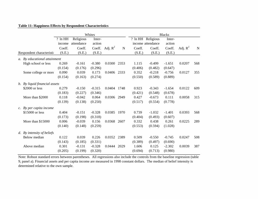
Table 11: Happiness Effects by Respondent Characteristics

? ln HH income

Religious attendance

Inter-action

? ln HH income

Religious attendance

Inter-action

Coeff. Coeff. Coeff. Adj. R2 N Coeff. Coeff. Coeff. Adj. R2 NRespondent characteristic (S.E.) (S.E.) (S.E.) (S.E.) (S.E.) (S.E.)

a. By educational attainmentHigh school or less 0.269 -0.161 -0.380 0.0300 2353 1.115 -0.499 -1.651 0.0207 568

(0.154) (0.176) (0.296) (0.406) (0.482) (0.647)Some college or more 0.090 0.039 0.173 0.0406 2333 0.352 -0.218 -0.756 0.0127 355

(0.154) (0.163) (0.274) (0.550) (0.589) (0.889)

b. By liquid financial assets$2000 or less 0.279 -0.150 -0.315 0.0404 1748 0.923 -0.343 -1.654 0.0122 609

(0.183) (0.227) (0.346) (0.421) (0.548) (0.678)More than $2000 0.118 -0.042 0.064 0.0306 2949 0.427 -0.673 0.111 0.0058 315

(0.139) (0.138) (0.250) (0.517) (0.554) (0.778)

c. By per capita income$15000 or less 0.404 -0.151 -0.328 0.0385 1970 0.739 -1.032 -1.401 0.0393 568

(0.173) (0.198) (0.318) (0.404) (0.493) (0.607)More than $15000 0.006 -0.039 0.156 0.0368 2607 0.332 0.438 0.261 0.0225 289

(0.140) (0.148) (0.259) (0.553) (0.594) (1.028)

d. By intensity of beliefsBelow median 0.122 0.039 0.226 0.0352 2389 0.509 -0.550 -0.745 0.0247 508

(0.143) (0.185) (0.331) (0.389) (0.497) (0.690)Above median 0.301 -0.131 -0.328 0.0444 2029 1.606 0.125 -2.302 0.0039 387

(0.205) (0.199) (0.320) (0.694) (0.713) (0.980)

Blacks

Note: Robust standard errors between parentheses. All regressions also include the controls from the baseline regression (table 9, panel a). Financial assets and per capita income are measured in 1998 constant dollars. The median of belief intensity is determined relative to the own sample.

Whites

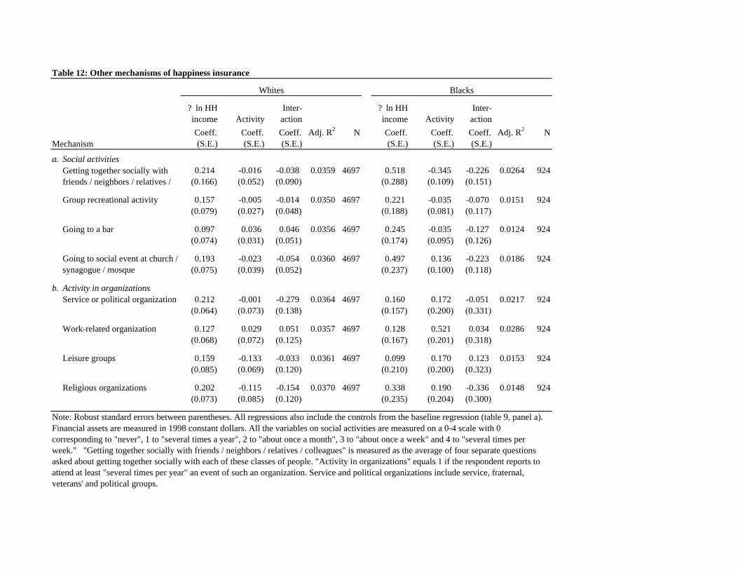
Table 12: Other mechanisms of happiness insurance

? ln HH income Activity

Inter-action

? ln HH income Activity

Inter-action

Coeff. Coeff. Coeff. Adj. R2 N Coeff. Coeff. Coeff. Adj. R2 NMechanism (S.E.) (S.E.) (S.E.) (S.E.) (S.E.) (S.E.)

a. Social activities0.214 -0.016 -0.038 0.0359 4697 0.518 -0.345 -0.226 0.0264 924

(0.166) (0.052) (0.090) (0.288) (0.109) (0.151)

Group recreational activity 0.157 -0.005 -0.014 0.0350 4697 0.221 -0.035 -0.070 0.0151 924(0.079) (0.027) (0.048) (0.188) (0.081) (0.117)

Going to a bar 0.097 0.036 0.046 0.0356 4697 0.245 -0.035 -0.127 0.0124 924(0.074) (0.031) (0.051) (0.174) (0.095) (0.126)

0.193 -0.023 -0.054 0.0360 4697 0.497 0.136 -0.223 0.0186 924(0.075) (0.039) (0.052) (0.237) (0.100) (0.118)

b. Activity in organizationsService or political organization 0.212 -0.001 -0.279 0.0364 4697 0.160 0.172 -0.051 0.0217 924

(0.064) (0.073) (0.138) (0.157) (0.200) (0.331)

Work-related organization 0.127 0.029 0.051 0.0357 4697 0.128 0.521 0.034 0.0286 924(0.068) (0.072) (0.125) (0.167) (0.201) (0.318)

Leisure groups 0.159 -0.133 -0.033 0.0361 4697 0.099 0.170 0.123 0.0153 924(0.085) (0.069) (0.120) (0.210) (0.200) (0.323)

Religious organizations 0.202 -0.115 -0.154 0.0370 4697 0.338 0.190 -0.336 0.0148 924(0.073) (0.085) (0.120) (0.235) (0.204) (0.300)

Whites Blacks

Getting together socially with friends / neighbors / relatives /

Note: Robust standard errors between parentheses. All regressions also include the controls from the baseline regression (table 9, panel a). Financial assets are measured in 1998 constant dollars. All the variables on social activities are measured on a 0-4 scale with 0 corresponding to "never", 1 to "several times a year", 2 to "about once a month", 3 to "about once a week" and 4 to "several times per week." "Getting together socially with friends / neighbors / relatives / colleagues" is measured as the average of four separate questions asked about getting together socially with each of these classes of people. "Activity in organizations" equals 1 if the respondent reports to attend at least "several times per year" an event of such an organization. Service and political organizations include service, fraternal, veterans' and political groups.

Going to social event at church / synagogue / mosque

Table 13: Religious affiliation and happiness effects of other life shocks

ShockReligious

attendanceInter-action Shock

Religious attendance

Inter-action

Coeff. Coeff. Coeff. Adj. R2 N Coeff. Coeff. Coeff. Adj. R2 NMechanism (S.E.) (S.E.) (S.E.) (S.E.) (S.E.) (S.E.)

a. Income shocksAll 0.191 -0.062 -0.108 0.0359 4697 0.794 -0.503 -1.160 0.0217 924

(0.110) (0.118) (0.202) (0.322) (0.375) (0.514)

Catholics 0.503 0.668 -0.574 0.0500 1129(0.306) (0.295) (0.520)

Other Christian 0.081 -0.219 0.049 0.0443 2437(0.154) (0.153) (0.267)

Not Christian 0.294 -0.063 -0.352 0.0301 1131(0.202) (0.300) (0.546)

b. Marital shocksAll 0.581 0.019 -0.150 0.0297 4697 -0.090 -0.467 0.344 0.0153 924

(0.120) (0.106) (0.237) (0.337) (0.288) (0.490)

Catholics 1.027 0.705 -1.059 0.0394 1129(0.311) (0.251) (0.560)

Other Christian 0.642 -0.165 -0.173 0.0359 2437(0.185) (0.137) (0.324)

Not Christian 0.476 0.076 -0.182 0.0279 1131(0.200) (0.278) (0.609)

c. Job shocksAll 0.219 -0.023 -0.057 0.0345 4697 0.518 -0.496 -0.264 0.0302 924

(0.113) (0.104) (0.206) (0.386) (0.285) (0.596)

Catholics 0.243 0.525 -0.100 0.0419 1129(0.316) (0.248) (0.541)

Other Christian 0.192 -0.199 0.072 0.0495 2437(0.159) (0.134) (0.263)

Not Christian 0.359 0.011 -0.530 0.0246(0.210) (0.283) (0.597)

d. Health shocksAll 0.252 -0.012 -0.047 0.0487 4697 0.131 -0.472 0.200 0.0281 924

(0.064) (0.106) (0.115) (0.183) (0.306) (0.300)

Catholics 0.051 0.606 0.283 0.0605 1129(0.169) (0.248) (0.298)

Other Christian 0.242 -0.226 -0.060 0.0554 2437(0.097) (0.139) (0.155)

Not Christian 0.305 0.169 -0.034 0.0475 1131(0.106) (0.282) (0.294)

Whites Blacks

Note: Robust standard errors between parentheses. All regressions also include the controls from the baseline regression (table 9, panel a), except the regressions for job shocks, which do not control for income shocks. Income shocks are measured as the log difference in real HH income, top and bottom coded at 100 log points from the sample-specific mean. Marital status shocks are 1 for those getting married, -1 for those whose marriage ends (though divorce, separation or death) and 0 for those without a marital status transition. Job shocks are 1 for those become employed, -1 for those leaving employment and zero for all others. Health shocks are changes in health status, self-reported on a 1-5 scale. The results for blacks are not broken down by religion because there are insufficient black Catholics and black non-Christians in the sample. Those who change religious affiliation are included in the "Other" group.

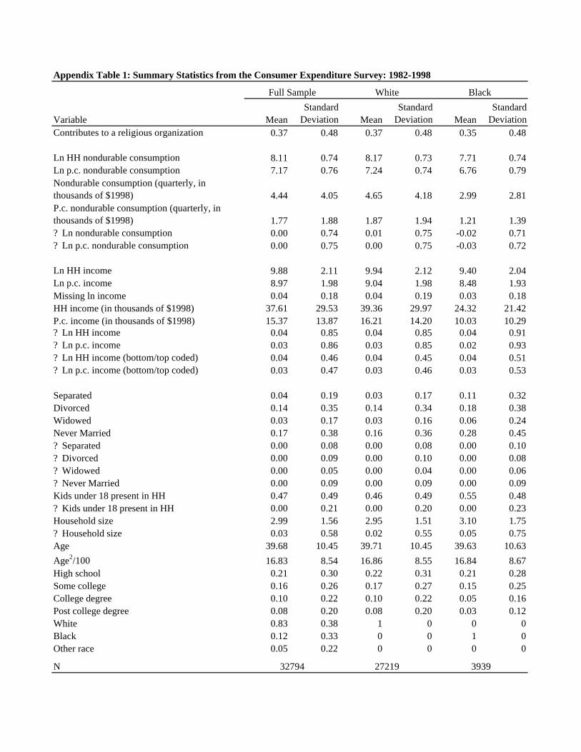
Appendix Table 1: Summary Statistics from the Consumer Expenditure Survey: 1982-1998

Variable MeanStandard

Deviation MeanStandard

Deviation MeanStandard

DeviationContributes to a religious organization 0.37 0.48 0.37 0.48 0.35 0.48

Ln HH nondurable consumption 8.11 0.74 8.17 0.73 7.71 0.74Ln p.c. nondurable consumption 7.17 0.76 7.24 0.74 6.76 0.79Nondurable consumption (quarterly, in thousands of $1998) 4.44 4.05 4.65 4.18 2.99 2.81P.c. nondurable consumption (quarterly, in thousands of $1998) 1.77 1.88 1.87 1.94 1.21 1.39? Ln nondurable consumption 0.00 0.74 0.01 0.75 -0.02 0.71? Ln p.c. nondurable consumption 0.00 0.75 0.00 0.75 -0.03 0.72

Ln HH income 9.88 2.11 9.94 2.12 9.40 2.04Ln p.c. income 8.97 1.98 9.04 1.98 8.48 1.93Missing ln income 0.04 0.18 0.04 0.19 0.03 0.18HH income (in thousands of $1998) 37.61 29.53 39.36 29.97 24.32 21.42P.c. income (in thousands of $1998) 15.37 13.87 16.21 14.20 10.03 10.29? Ln HH income 0.04 0.85 0.04 0.85 0.04 0.91? Ln p.c. income 0.03 0.86 0.03 0.85 0.02 0.93? Ln HH income (bottom/top coded) 0.04 0.46 0.04 0.45 0.04 0.51? Ln p.c. income (bottom/top coded) 0.03 0.47 0.03 0.46 0.03 0.53

Separated 0.04 0.19 0.03 0.17 0.11 0.32Divorced 0.14 0.35 0.14 0.34 0.18 0.38Widowed 0.03 0.17 0.03 0.16 0.06 0.24Never Married 0.17 0.38 0.16 0.36 0.28 0.45? Separated 0.00 0.08 0.00 0.08 0.00 0.10? Divorced 0.00 0.09 0.00 0.10 0.00 0.08? Widowed 0.00 0.05 0.00 0.04 0.00 0.06? Never Married 0.00 0.09 0.00 0.09 0.00 0.09Kids under 18 present in HH 0.47 0.49 0.46 0.49 0.55 0.48? Kids under 18 present in HH 0.00 0.21 0.00 0.20 0.00 0.23Household size 2.99 1.56 2.95 1.51 3.10 1.75? Household size 0.03 0.58 0.02 0.55 0.05 0.75Age 39.68 10.45 39.71 10.45 39.63 10.63Age2/100 16.83 8.54 16.86 8.55 16.84 8.67High school 0.21 0.30 0.22 0.31 0.21 0.28Some college 0.16 0.26 0.17 0.27 0.15 0.25College degree 0.10 0.22 0.10 0.22 0.05 0.16Post college degree 0.08 0.20 0.08 0.20 0.03 0.12White 0.83 0.38 1 0 0 0Black 0.12 0.33 0 0 1 0Other race 0.05 0.22 0 0 0 0

N

Full Sample White Black

32794 27219 3939

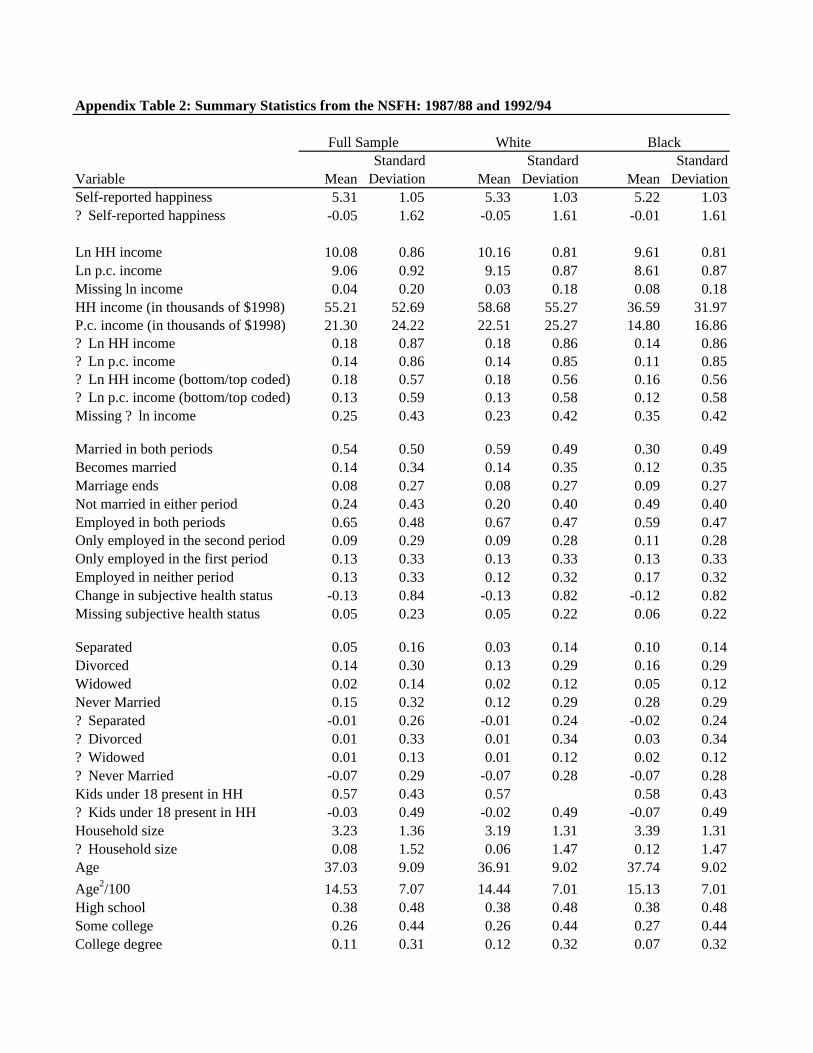
Appendix Table 2: Summary Statistics from the NSFH: 1987/88 and 1992/94

Variable MeanStandard

Deviation MeanStandard

Deviation MeanStandard

DeviationSelf-reported happiness 5.31 1.05 5.33 1.03 5.22 1.03? Self-reported happiness -0.05 1.62 -0.05 1.61 -0.01 1.61

Ln HH income 10.08 0.86 10.16 0.81 9.61 0.81Ln p.c. income 9.06 0.92 9.15 0.87 8.61 0.87Missing ln income 0.04 0.20 0.03 0.18 0.08 0.18HH income (in thousands of $1998) 55.21 52.69 58.68 55.27 36.59 31.97P.c. income (in thousands of $1998) 21.30 24.22 22.51 25.27 14.80 16.86? Ln HH income 0.18 0.87 0.18 0.86 0.14 0.86? Ln p.c. income 0.14 0.86 0.14 0.85 0.11 0.85? Ln HH income (bottom/top coded) 0.18 0.57 0.18 0.56 0.16 0.56? Ln p.c. income (bottom/top coded) 0.13 0.59 0.13 0.58 0.12 0.58Missing ? ln income 0.25 0.43 0.23 0.42 0.35 0.42

Married in both periods 0.54 0.50 0.59 0.49 0.30 0.49Becomes married 0.14 0.34 0.14 0.35 0.12 0.35Marriage ends 0.08 0.27 0.08 0.27 0.09 0.27Not married in either period 0.24 0.43 0.20 0.40 0.49 0.40Employed in both periods 0.65 0.48 0.67 0.47 0.59 0.47Only employed in the second period 0.09 0.29 0.09 0.28 0.11 0.28Only employed in the first period 0.13 0.33 0.13 0.33 0.13 0.33Employed in neither period 0.13 0.33 0.12 0.32 0.17 0.32Change in subjective health status -0.13 0.84 -0.13 0.82 -0.12 0.82Missing subjective health status 0.05 0.23 0.05 0.22 0.06 0.22

Separated 0.05 0.16 0.03 0.14 0.10 0.14Divorced 0.14 0.30 0.13 0.29 0.16 0.29Widowed 0.02 0.14 0.02 0.12 0.05 0.12Never Married 0.15 0.32 0.12 0.29 0.28 0.29? Separated -0.01 0.26 -0.01 0.24 -0.02 0.24? Divorced 0.01 0.33 0.01 0.34 0.03 0.34? Widowed 0.01 0.13 0.01 0.12 0.02 0.12? Never Married -0.07 0.29 -0.07 0.28 -0.07 0.28Kids under 18 present in HH 0.57 0.43 0.57 0.58 0.43? Kids under 18 present in HH -0.03 0.49 -0.02 0.49 -0.07 0.49Household size 3.23 1.36 3.19 1.31 3.39 1.31? Household size 0.08 1.52 0.06 1.47 0.12 1.47Age 37.03 9.09 36.91 9.02 37.74 9.02Age2/100 14.53 7.07 14.44 7.01 15.13 7.01High school 0.38 0.48 0.38 0.48 0.38 0.48Some college 0.26 0.44 0.26 0.44 0.27 0.44College degree 0.11 0.31 0.12 0.32 0.07 0.32

Full Sample White Black

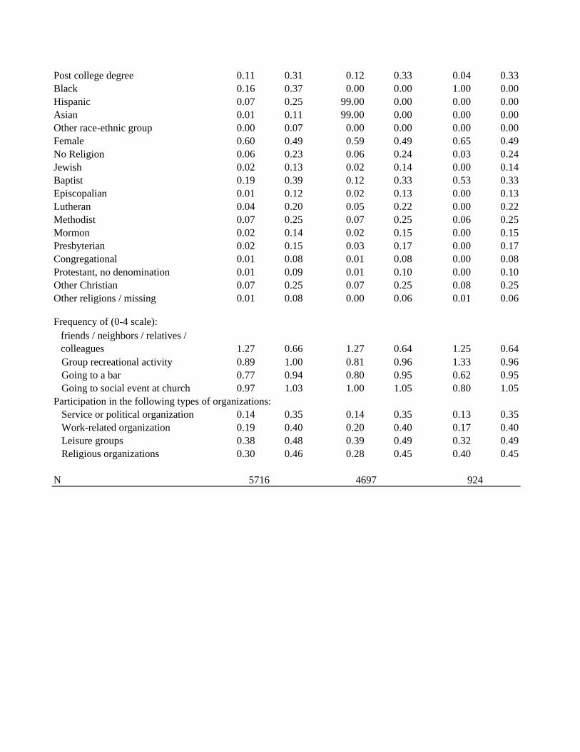
Post college degree 0.11 0.31 0.12 0.33 0.04 0.33Black 0.16 0.37 0.00 0.00 1.00 0.00Hispanic 0.07 0.25 99.00 0.00 0.00 0.00Asian 0.01 0.11 99.00 0.00 0.00 0.00Other race-ethnic group 0.00 0.07 0.00 0.00 0.00 0.00Female 0.60 0.49 0.59 0.49 0.65 0.49No Religion 0.06 0.23 0.06 0.24 0.03 0.24Jewish 0.02 0.13 0.02 0.14 0.00 0.14Baptist 0.19 0.39 0.12 0.33 0.53 0.33Episcopalian 0.01 0.12 0.02 0.13 0.00 0.13Lutheran 0.04 0.20 0.05 0.22 0.00 0.22Methodist 0.07 0.25 0.07 0.25 0.06 0.25Mormon 0.02 0.14 0.02 0.15 0.00 0.15Presbyterian 0.02 0.15 0.03 0.17 0.00 0.17Congregational 0.01 0.08 0.01 0.08 0.00 0.08Protestant, no denomination 0.01 0.09 0.01 0.10 0.00 0.10Other Christian 0.07 0.25 0.07 0.25 0.08 0.25Other religions / missing 0.01 0.08 0.00 0.06 0.01 0.06

Frequency of (0-4 scale):friends / neighbors / relatives / colleagues 1.27 0.66 1.27 0.64 1.25 0.64

Group recreational activity 0.89 1.00 0.81 0.96 1.33 0.96 Going to a bar 0.77 0.94 0.80 0.95 0.62 0.95 Going to social event at church 0.97 1.03 1.00 1.05 0.80 1.05Participation in the following types of organizations: Service or political organization 0.14 0.35 0.14 0.35 0.13 0.35 Work-related organization 0.19 0.40 0.20 0.40 0.17 0.40 Leisure groups 0.38 0.48 0.39 0.49 0.32 0.49 Religious organizations 0.30 0.46 0.28 0.45 0.40 0.45

N 5716 4697 924