intech-aloha and csma in wireless ad hoc networks

Chapter 1

Comparison of the Maximal Spatial Throughput of

Aloha and CSMA in Wireless Ad-Hoc Networks

B. Blaszczyszyn, P. Mühlethaler and S. Banaouas

Additional information is available at the end of the chapter

http://dx.doi.org/10.5772/53264

Provisional chapter

Comparison of the Maximal Spatial Throughput of

Aloha and CSMA in Wireless Ad-Hoc Networks

B. Blaszczyszyn, P. Mühlethaler and S. Banaouas

Additional information is available at the end of the chapter

10.5772/53264

1. Introduction

Multiple communication protocols are used to organize transmissions from several sources (network

nodes) in such a way that scheduled transmissions are likely to be successful. Aloha is one of the most

common examples of such a protocol. A major characteristic of Aloha is its great simplicity: the core

concept consists in allowing each source to transmit a packet and back-off for some random time before

the next transmission, independently of other sources. The main idea of the Carrier-Sense Multiple

Access technique (CSMA) is to listen before sending a packet. CSMA is perhaps the most simple and

popular access protocol that integrates some collision avoidance mechanism.

Simple classical models allow one to analyze Aloha and CSMA (see [1, 2]). They show that CSMA

significantly outperforms Aloha as long as the maximum propagation delays between network nodes

remain small compared to the packet transmission delays. However these models are not suitable

for a wireless multihop network context, as they do not take into account the specificity of the

radio propagation of the signal. Consequently, they cannot capture the spatial reuse effect (i.e., the

possibility of simultaneous successful wireless transmissions) which is a fundamental property of

multihop wireless communications.

Intuitively, it could be inferred that the collision avoidance embedded in CSMA should provide a greater

spatial throughput than Aloha’s purely random technique. Despite the large number of studies which

evaluate Aloha and CSMA, to the authors’ best knowledge there is no “fair” comparison of the spatial

throughput of the two schemes in wireless multihop ad-hoc networks1. The aim of this paper is to carry

out such a comparison and to quantify the gain in spatial throughput of CSMA over Aloha. We also

study the effect of the various parameters on the performances. To do so, we model the geographic

locations of network nodes by a planar Poisson point process and use the standard power-law path-loss

1 [3] is the only similar study we know of but we explain in this paper why the comparison presented in [3] is not, in our opinion,

“fair” according to us.

©2012 Blaszczyszyn et al., licensee InTech. This is an open access chapter distributed under the terms of theCreative Commons Attribution License (http://creativecommons.org/licenses/by/3.0), which permits unrestricteduse, distribution, and reproduction in any medium, provided the original work is properly cited.© 2012 Blaszczyszyn et al.; licensee InTech. This is an open access article distributed under the terms of theCreative Commons Attribution License (http://creativecommons.org/licenses/by/3.0), which permitsunrestricted use, distribution, and reproduction in any medium, provided the original work is properly cited.

2 Mobile Ad-Hoc Networks

function of the Euclidean distance to model the mean attenuation of the signal power. Regarding radio

channel conditions, we consider both standard Rayleigh and negligible fading. We use a SINR model

in which each successful transmission requires that the receiver is covered by the transmitter with a

minimum SINR.

For Aloha (both slotted and non-slotted), the above model lends itself to mathematical analysis as shown

in [4, 5]. We adopt use and develop this approach and use simulations (which confirm the analytical

results) to evaluate and optimize the performances of Aloha. The performance of the CSMA in the

previous model is very complex thus we use simulations to study it.

The main contribution of this paper is the analysis and comparison of the performances of slotted,

non-slotted Aloha and CSMA, all optimized to maximize the rate of successful transmissions, under

various radio propagation assumptions (path-loss exponent, fading conditions). Our main findings of

this analysis are:

• CSMA always outperforms slotted Aloha, which in turn outperforms non-slotted Aloha. In a

moderate path-loss scenario (path-loss exponent equal to 4), without fading and the SINR level

required for capture equal to 10, CSMA offers approximately a 2.4 times larger rate of successful

transmissions than slotted Aloha and approximately a 3.2 times larger rate than non-slotted Aloha.

• The advantage of using CSMA is slightly reduced by increasing path-loss decay.

• This advantage is significantly reduced by the existence of fading since CSMA is much more

sensitive to channel randomness than Aloha. In particular, for Rayleigh fading the above comparison

of CSMA to slotted and non-slotted Aloha gives the ratios 1.7 and 2.3, respectively.

• The advantage of using CSMA increases with the SINR capture level.

• The above observations are valid when the transmissions are roughly scheduled to nearest neighbors

and all the three MAC schemes are optimally tuned. This optimal tuning results in scheduling

each node for transmission for about 8%, 6% and 4% of the time, for CSMA, slotted and

non-slotted Aloha, respectively. These values do not depend on the network density, provided the

nearest-neighbor receiver scheduling is used.

• The optimal tuning of CSMA is obtained by fixing the carrier-sensing power level (used to detect if

the channel is idle) to about 8% of the useful signal power received at the nearest neighbor distance.

This makes the transmissions successful with a high probability (from 0.8 to 0.95). Both smaller

and larger values of the carrier-sensing threshold lead to essentially suboptimal performance of

CSMA and sometimes even comparable to that of slotted Aloha. This might explain the apparent

contradiction of our results to those of [3], which indicate similar performance of Aloha and CSMA.

This paper also contributes to the development of the mathematical tools for Aloha by showing that the

so-called spatial contention factor cf [6], appearing in the Laplace-transform characterization of the

interference, is larger in non-slotted Aloha than in slotted Aloha under the same channel assumptions,

by a factor that depends in a simple, explicit way only on the path-loss exponent; cf. Fact 3.2. We also

suggest the usage of the Bromwich contour inversion integral, developed in [7], to evaluate the coverage

probability in the no-fading case; cf. Fact 3.6.

In this paper we will not take into account second order factors such as the back-off strategy in CSMA

or guard intervals in slotted Aloha. We will briefly discuss these factors at the end of the paper to show

that they cannot change the order of magnitude of the comparison between Aloha and CSMA.

The remaining part of this paper is organized as follows. In Section 1.1) we recall some previous

studies of Aloha and CSMA. Section 2 introduces the model: distribution of nodes, channel and capture

assumptions. It also describes in more detail the three MAC protocols studied in this paper. In Section 3

Wireless Ad-Hoc Networks4

Comparison of the Maximal Spatial Throughput of Aloha and CSMA in Wireless Ad-Hoc Networks 3

10.5772/53264

we present our analysis tools. Section 4 provides our findings regarding the performance of the MAC

protocols considered. The conclusions are presented in Section 5.

1.1. Related work

Aloha and Time Division Multiple Access (TDMA) are the oldest multiple access protocol. Aloha,

which is the “mother” of random protocols, was born in the early seventies, the seminal work

describing Aloha [8] being published in 1970. Since that time it has become widespread in various

implementations. The essential simplicity of Aloha also allows for simple analysis. A first, and now

widely taught result regarding the ratio of successful transmissions (cf. e.g [2, 4.2]) was obtained

assuming an aggregate, geometry-less process of transmissions following a temporal Poisson process,

with some overlapping of two or more packet transmissions necessarily leading to a collision. In this

model, the ratio of successful transmissions can reach 1/(2e) ≈ 18%, when the scheme is optimized

by appropriate tuning of the mean back-off time (intensity of the Poisson process). It was also shown,

that this performance can be multiplied by 2 in slotted-Aloha, when all the nodes are synchronized and

can send packets only at the beginning of some universal time slots.

Although Aloha was primarily designed to manage wireless networks, the lack of a geometric

representation of node locations in the above model makes it unsuitable for wireless networks. To the

authors’ best knowledge, it is in the paper by Nelson and Kleinrock [9] that Aloha was first explicitly

studied in a wireless context. The authors showed that under ideal circumstances with slotted Aloha the

“expected fraction of terminals in the network that are engaged in successful traffic in any slot does not

exceed 21%”. Despite the very simple on-off wireless propagation model used in the paper, this result,

as we will show, is surprisingly close to the results that can be obtained using more recent and more

sophisticated, physical propagation and interference models (cf. [4, 6]) in the case of the fading-less

channel model with the mean path-loss decay equal to 3.5. The key element of this latter approach is

the explicit formula of the Laplace transform of the interference created by a Poisson pattern of nodes

using Aloha. This analysis was recently extended to non-slotted Aloha in [5]. We adopt this approach

and slightly extend it in the present paper.

In the widely referenced paper [10] another simplified propagation model was used to study local

interactions of packet transmissions and the stability of spatial Aloha.

CSMA was studied in the 70s in [1] and in the 90s in articles such as [11]. In these studies, the spatial

reuse is usually not considered. However a few articles such as [12–14] take it into account by modeling

carrier sensing with a graph. Nodes within carrier sense are linked vertices in this graph. However this

model only approximates the carrier-sensing and the capture effect. [15] uses the same model for

CSMA to study the per-flow throughput in the network. Other simplified models of the carrier sensing

and capture effect are proposed in [16, 17].

At the end of the 90s, an original and well referenced study tried to capture the behaviour of the IEEE

802.11 distributed medium access algorithm [18]. Although this study represented a step forward in the

analysis of the IEEE 802.11 collision avoidance mechanism, [18] did not include an accurate model to

capture interference. Thus the spatial throughput of IEEE 802.11 cannot be analyzed with this model.

Although numerous papers are actually using models close to that of [18], they are all unable to compute

the spatial throughput of IEEE 802.11.

In contrast to [18], [19] studies the behaviour of a CSMA network using a more realistic model for

interference and for the capture of packets. However [19] cannot obtain closed formulas and [19] is

actually a semi analytical model based on a Markov chain. Moreover this model can only handle a few

dozen nodes. Thus it cannot easily compute average performance or investigate the effect of the network

parameters. New models have recently appeared such as [20]. These models use the Matern hard core

Comparison of the Maximal Spatial Throughput of Aloha and CSMA in Wireless Ad-Hoc Networkshttp://dx.doi.org/10.5772/53264

5


process to model the pattern of simultaneously transmitting nodes in a CSMA network. These models,

which allow the spatial throughput to be evalutated, have many flaws. First, CSMA is not accurately

modeled by the Matern hard core process. Secondly the interference is also only approximated. Lastly

the formulas obtained in these models to obtain the throughput are complex and it is difficult to use

them to optimize the protocol when we vary the network parameters. Despite the many papers trying

to analyze the performance of CSMA with spatial reuse, we believe that none of these papers offers

a method for precise and straightforward evaluation of the gain from using the collision avoidance

mechanism of CSMA, in the same framework (infinite Poisson ad-hoc network) in which spatial Aloha

can been analyzed. Thus, for this paper we chose to rely on simulations to estimate the performance of

CSMA. We believe that, for our purpose, this approach offers a faster, more accurate method which is

also easy to implement.

We also want to recall the original geometric approach, also by Nelson and Kleinrock, presented in [3].

Their seminal paper presents a comparison of the performance of Aloha and CSMA in the geometric

setting with the simple on-off wireless propagation model. Such a comparison is also the goal of our

present study which however uses a more realistic propagation and interference model (see above). Our

conclusions appear to differ from those of [3], where the performance of CSMA is found comparable to

Aloha. We show that CSMA, with an appropriately tuned sensing threshold, can essentially outperform

Aloha. The reason for this difference is presumably not due to the different wireless channel models,

but primarily because of a sub-optimal tuning of the CSMA in [3], consisting of too small a sensing

range (taken to be equal to the transmission range). In that sense [3] does not provide a fair comparison

of the spatial throughput of Aloha and CSMA whereas, we believe, our paper does. [21] also compares

Aloha and CSMA but only in terms of outage probability; [21] does not derive the density of successful

transmission.

2. Models

In this section we present the models, which will be used to evaluate and compare the performance of

the CSMA and Aloha MAC schemes.

2.1. Distribution of nodes and channel model

The model that we use here was proposed in [4]; we call it the Poisson Bipole model. It assumes that

the nodes of a Mobile Ad hoc NETwork (MANET) are distributed on the infinite plane according to a

homogeneous, planar Poisson point process of intensity λ nodes per unit surface area (say per square

meter). Each node of this network transmits a packet to its own dedicated receiver located at random

within a distance r meters from it, which is not a part of the Poisson point process. In this paper we

choose r = a/√

λ, for some constant a > 0, i.e. of the order of the mean distance to the nearest

neighbor in a Poisson point process of intensity λ. This choice mimics the nearest neighbor scenario.

We also assume that every node has always a pending packet to send. We believe that this assumption

represents the behaviour of a loaded network and allows us to compute the maximum throughput of the

network in a multihop context.

Using the formalism of the theory of point processes, we will say that a snapshot of the MANET

can be represented by an independently marked Poisson point process (P.p.p) Φ = {(Xi, yi)}, where

the locations of nodes Φ = {Xi} form a homogeneous P.p.p. on the plane, with an intensity of λ,

and where the mark yi denotes the location of the receiver for node Xi. We assume here that one

receiver is associated with only one transmitter and that, given Φ, the vectors {Xi − yi} are i.i.d with

|Xi − yi| = r.



10.5772/53264

We assume that whenever node Xi ∈ Φ transmits a packet it emits a unit-power signal that is propagated

and reaches any given location y on the plane with power equal to F/l(|Xi − y|).

l(u) = (Au)β for A > 0 and β > 2 (1)

and | · | denotes the Euclidean distance on the plane. Regarding the distribution of the random variable

F, called for simplicity fading, we will consider two cases:

• constant F ≡ 1, called the no fading case,

• exponential F of parameter 1; this corresponds to the Rayleigh fading in the channel.

2.2. Successful transmission

It is natural to assume that transmitter Xi successfully transmits a given packet of length B to its receiver

yi within the time interval [u, u + B] if

SIR =F/l(|Xi − yi|)

I≥ T , (2)

where T is some signal-to-interference (SIR) threshold and where I is the average interference suffered

by the receiver yi during this packet transmission interval

I =1

B

∫ u+B

uI(t) dt , (3)

with

I(t) = ∑Xj∈Φ,Xj 6=Xi

Fj,yi/l(|Xj − yi|)1I(Xj transmits at time t) . (4)

Note that taking (2) as the successful transmission condition, we ignore any external noise. This is a

reasonable assumption if the noise is significantly smaller than the interference power I, which is the

case in our setting.

2.3. MAC protocols

We will assume a saturated traffic model, i.e, that each node always has a packet to transmit to its

receiver. The times at which any given node can transmit are decided by the Medium Access Protocol

(MAC). In this paper we study three MAC protocols: CSMA, slotted Aloha and non-slotted Aloha.

2.3.1. CSMA

The basic rule of CSMA is very simple: each node ready to transmit a packet listens first to the channel

and transmits only if it finds the channel idle. Otherwise it waits for the channel to be idle and further

postpones its transmission attempt for an additional random "back-off" time used to select a single node

among the nodes blocked by the previous transmission. We assume that this random "back-off" time is


7


very small and we do not consider it in this study. This assumption is true if the ratio of the propagation

plus detection time over the transmission time of the packet is very small. We discuss at the end of the

article how to introduce corrective terms if propagation and detection times are not negligle.

To decide whether the channel is idle, the sender node computes the interference it receives I′. If I′ ≤ θ,

where θ is the carrier-sense threshold then the channel is “idle” otherwise it is busy. The carrier-sense

threshold θ is the main, and in our model, the only parameter that will be tuned to maximize the density

of successful transmissions and thus optimize the performance of the CSMA.

2.3.2. Slotted Aloha

Slotted Aloha supposes that all the network nodes are perfectly synchronized to some time slots (each

of the length B of the packet, common for the whole network) and transmit packets according to the

following rule: each node, at each time slot independently tosses a coin with some bias p which will be

referred to as the Aloha medium access probability (Aloha MAP); it sends the packet in this time slot if

the outcome is heads and does not transmit otherwise.

The Aloha MAP p is the main parameter to be tuned to optimize the access (see a precise description

of the stationary space-time model in [5]).

2.3.3. Non-Slotted Aloha

In non-slotted Aloha all the network nodes independently, without synchronization, send packets (of

the same duration B) and then back off for some exponential random time of mean ε. In a more

formal description of this mechanism one assumes that, given a pattern of network nodes, the temporal

patterns of their retransmission are independent (across the nodes) renewal processes with the generic

inter-arrival time equal to B+ E where E is exponential (back-off) with mean ε. A precise description of

this stationary space-time model, called the Poisson-renewal model of non-slotted Aloha can be found

in [5]. The analysis of this Poisson-renewal model of Aloha is feasible although it does not lead to

simple closed formulas. In [5] another model, called the Poisson rain model, of non-slotted Aloha has

been proposed. The main difference with respect to the scenario considered above is that the nodes Xi

and their receivers yi are not fixed in time. Instead, we may think of these nodes as being “born” at some

time Ti transmitting a packet during time B and “disappearing” immediately after. The joint space-time

distribution of node locations and transmission instances Ψ = {(Xi, Ti)} is modeled by a homogeneous

Poisson p.p. in 2 + 1 dimensions with intensity λs = λB/(ε + B). It might be theoretically argued

that the Poisson rain model is a good approximation of the Poisson-renewal model when the density of

nodes λ is large, and the time instances at which a given node retransmits are very sparse. Indeed, the

performance of the Poisson-renewal model is shown in [5] to be very close to that of the Poisson rain

model. Thus, in our analytical study of non-slotted Aloha we will use the results regarding the latter for

simplicity, while in our simulations we use the former.

2.4. Network performance under a given MAC

MAC protocols are supposed to create some space-time patterns of active (transmitting) nodes that

increase the chances of successful transmissions. MAC optimization consists in finding the right

trade-off between the density of active nodes and the probability that the individual transmissions are

successful.

The first step of the analysis of the above trade-off problem consists in evaluating how much a given

MAC protocol contends to the channel; i.e., how many packets it attempts to send per node and per



10.5772/53264

unit of time. In homogeneous models this can be captured by the average fraction of time a typical

node is authorized to transmit. We will denote this metric by τ. By space-time homogeneity, τλ is the

spatial density of active nodes at any given time and thus τ can also be interpreted as the probability

that a typical node of the MANET is active at a given time. In what follows we will call it thechannel

occupation parameter. The way it depends on the basic (tunable) MAC parameters will be explained

later on.

A complete evaluation of the performance of a MAC protocol must establish the fraction of successful

authorized transmissions. We will denote by pc the probability that a typical transmission by a typical

node is successful (given this node was authorized by the MAC to transmit). We call it the coverage

probability for short. By (2) we have

pc = P0{ F ≥ l(r)TI } , (5)

where the probability P0 corresponds to the distribution of the random variables for a typical node

during its typical transmission; this can be formalized using the Palm theory for point processes. This

expression will be the basis of our analytical evaluation of the coverage probability for both slotted and

non-slotted Aloha in Section 3.3. We can notice that I is independent of F in (5) because our MAC

schemes do not schedule transmissions according to the channel conditions at the receivers.

We define the optimal performance of a given MAC scheme as the situation where the mean number

of successful transmissions per unit of surface and unit of time τλpc, called the density of successful

transmissions, is maximized. For a given MANET density λ, this is equivalent to maximizing τpc,

which can be interpreted as the probability that a typical node is transmitting at a given time and this

transmission is successful. Following this interpretation, we call τpc the mean throughput per node.

It will be analytically evaluated for both Aloha schemes and estimated by simulations for Aloha and

CSMA MAC.

3. Analysis tools

3.1. Simulation scenarios

Our simulations are carried out in a square of 1000 m×1000 m in which we generate a Poisson sample

of MANET nodes with intensity λ = 0.001 nodes per square meter. For each MANET node we

generate the location of its receiver uniformly on the circle of radius r = a√

1000 m centered on this

node. To avoid side effects, we consider a toroidal metric on this square. (Recall that, roughly speaking,

rectangular torus is a rectangle whose opposite sites are “identified”.) Given this metric we consider the

distance dependent path-loss model (1) with some given path-loss exponent β and A = 1.

Typically β is larger than 2 and smaller than 6. 2 corresponds to free space propagation and 6 is for

situations with a lot of obstacles and reflections. We will use the default value β = 4; in [22] the

Walfishch-Ikegami model provides β = 3.8. However in some experiments, we try different values of

β. For each pair of nodes we generate an independent copy of the exponential variable F in the case of

Rayleigh fading or take F ≡ 1 in the no-fading case. Unless explicitly specified, our default value of

the SIR threshold is T = 10 which is a widely used value.

For a given distribution of nodes we run the dynamic simulation for each of the three MAC schemes

described in Section 2.3 with some particular choice of their main parameters: the carrier-sense

threshold θ for CSMA, MAP p for slotted Aloha and mean back-off time for non-slotted Aloha. The


9


packet transmission duration is always B = 1 unit of time. We count both the total number of packet

transmissions and the number of successful transmissions during the simulation, whose total time is

4000 units of time. For CSMA, as already said, we ignore the time spent in back-off when a node, after

having sensed the channel busy, finds the channel idle again before attempting another transmission. In

the simulations we use very small back-off times to select the transmitting nodes and we neglect the time

actually spent in these back-offs. Since each packet transmission takes B = 1 unit of time, dividing the

number of transmissions by the simulation time and by the number of MANET nodes in the square, we

obtain the one-network-sample estimators of, respectively, the average fraction τ of time a typical node

is authorized to transmit and the mean throughput per node τpc. We repeat the above experiment for 10

random choices of the network and take the empirical means of the above one-sample estimators. The

error-bars in all simulation results correspond to a confidence interval of 95%. We use a home-made

event-driven simulator specially dedicated to our simulation problem. This simulatot provides much

faster simulation results than the ones we would obtain with on the shelf simulation tools.

3.2. Analytical results for Aloha MAC

The analytical results for Aloha are based on the (simple) calculation of the average fraction of time

a typical node is authorized to transmit τ and a (more involved) calculation of the Laplace transform

of the interference I that is the only variable of “unknown” distribution in the expression (5) of the

coverage probability pc.

3.2.1. Channel Occupation τ

It is straightforward to see that in slotted Aloha τ = p. In the Poisson-renewal model of non-slotted

Aloha τ = B/(B + ε); i.e., the ratio between the packet duration time and the mean inter-transmission

time.

3.2.2. Interference Distribution

The basic observation allowing explicit analysis of the coverage probability for all our Poisson models

of Aloha is that the distribution of the interference I under the Palm probability P0 in (5) corresponds

to the distribution of the interference “seen” by an extra receiver added to the original MANET pattern

(say at the origin) during an arbitrary period of time of length B (say in [0, B]). This is a consequence

of Slivnyak’s theorem.

Moreover, note that in the slotted Aloha MAC the interference I(t) = I in (3) does not vary during

the packet transmission and consequently I = I. Furthermore, note that the pattern of nodes Xj, which

emit at a given time slot and interfere with a given packet transmission (cf. expression (4)) is a Poisson

p.p. of intensity pλ. This is a consequence of the independent MAC decisions of Aloha. The general

expression of the Laplace transform LI of I, which in this case is a Poisson shot-noise variable, is

known explicitly. Here we recall the expressions for the special cases of interest.

Fact 3.1. For the slotted Aloha model with path-loss function (1) and a general distribution of fading

F with mean 1 we have:

LI(ξ) = exp{−λτA−2ξ2/βκ} , (6)

where κ ≥ 0 is some constant depending only on the path-loss exponent and the distribution of the

fading F. In particular



10.5772/53264

• κ = πΓ(1 − 2/β) in the no-fading scenario F ≡ 1,

• κ = 2πΓ(2/β)Γ(1 − 2/β)/β with Rayleigh fading.

The constant κ was evaluated in [4] for Rayleigh fading and in [6], for the no-fading scenario, where

the name spatial contention factor was proposed for this constant. Γ() is the classical gamma function.

Regarding the distribution of the averaged interference I in non-slotted Aloha, we have the following

new general result.

Fact 3.2. Assume the Poisson rain model of non-slotted Aloha with space-time intensity of packet

transmissions λs = λτ and the path-loss function (1). Assume a general distribution of fading F. Then

the Laplace transform L I(ξ) of the averaged interference I is given by (6) with the spatial contention

factor κ = κnon−slotted equal to

κnon−slotted =2β

2 + βκslotted ,

where κslotted is the spatial contention factor evaluated for slotted Aloha under the same channel

assumptions.

Proof. By (3), (4) and exchanging the order of integration and summation we express I in the following

form

I = ∑Xj∈Φ,Xj 6=Xi

Fj,yiHj/l(|Xj − yi|) ,

where Hj = 1B

∫ u+Bu 1I(Xj emits at time t) dt. In the Poisson rain model we have

1I(Xj emits at time t) = 1I(t − B ≤ Tj ≤ t), where Tj is the time at which Xj starts emitting.

Integrating the previous function we obtain Hj = h(Tj), where h(s) = (B − |s|)+/B and t+ =max(0, t). Consequently, for the Poisson rain model represented by Poisson p.p. Ψ = {Xi, Ti} (cf.

Section 2.3.3) the averaged interference at the typical transmission receiver is equal in distribution to

Idistr.= ∑

Xj ,Tj∈Ψ

Fjh(Tj)/l(|Xj|) ,

where Fj are i.i.d. copies of the fading. Using the general expression for the Laplace transform of the

Poisson shot-noise we obtain for the path-loss function (1)

L I(ξ) = exp{

−2πλs

∫ ∞

−∞

∫ ∞

0r(

1 −LF

(

ξh(t)(Ar)−β)

)

dr dt}

,

where LF is the Laplace transform of F. Substituting r := Ar(ξh(t))−1/β for a given fixed t in the

inner integral we factorize the two integrals and obtain L I(ξ) = exp{−2πλs A−2ξ2/βζκ}, where

ζ =∫ ∞

−∞(h(t))2/β dt and κ =

∫ ∞

0 r(1 −LF(r−β)) dr. A direct calculation yields ζ = 2β/(2 + β).

This completes the proof.


11


Remark 3.3. Regarding the ratio of the spatial contention parameters ζ = ζ(β) = 2β/(2 + β),that can be seen as the cost of non-synchronization in Aloha (cf Remark 3.5 below), note that in

the free-space propagation model (where β = 2) it is equal to 1 (which means that the interference

distribution, and so coverage probability, in slotted and non-slotted Aloha are the same). Moreover,

ζ(β) increases with the path-loss exponent and asymptotically (for β = ∞) approaches the value 2.

This was only conjectured in [5].

3.3. Coverage probability

Evaluating pc from (5) is straightforward in the case of Rayleigh fading. Indeed, with F independent of

I one has P0{ F ≥ l(r)TI } = E

0[exp{−l(r)TI}] = L I(l(r)T). By Facts 3.1 and 3.2 we have the

following result.

Fact 3.4. For the Aloha model with the path-loss function (1) and Rayleigh fading

pc = exp{

−λτr2T2/βκ}

, (7)

where

• κ = 2πΓ(2/β)Γ(1 − 2/β)/β for slotted Aloha and

• κ = 4πΓ(2/β)Γ(1 − 2/β)/(2 + β) for non-slotted Aloha.

Remark 3.5. Note that due to our parametrization r = a/√

λ (which mimics the nearest-neighbor

receiver model), the maximal mean throughput per node τpc is achieved (in slotted or non-slotted

Aloha with Rayleigh fading) for τ = τ∗ = κ−1a−2T−2/β and it is equal to τ∗/e. In particular, by

Fact 3.2, non-slotted Aloha achieves ζ = ζ(β) times smaller maximal throughput than slotted Aloha,

where ζ is the cost of non-synchronization in Aloha. The dependence of this cost on β is analyzed

in Remark 3.3. Here, note only that the well-known result obtained for the simplified collision model

with on-off path-loss function, and saying that slotted Aloha offers two times greater throughput than

non-slotted Aloha (see [2, Section 4.2]) corresponds in our model to the infinite path-loss exponent;

ζ(∞) = 2.

In the case of a general distribution of fading the evaluation of pc from the Laplace transform L I is not

so straightforward. Some integral formula, based on the Plancherel-Parseval theorem, can be used when

F has a square integrable density. This approach however does not apply to the no-fading case F ≡ 1.

Here we suggest another, numerical approach, based on the Bromwich contour inversion integral and

developed in [7], which is particularly efficient in this case.

Fact 3.6. For Aloha model with constant fading F ≡ 1 we have

pc =2 exp{d/(Tl(r))}

π

∫

∞

0R(1 −L I(d + iu)

d + iu

)

cos ut du , (8)

where d > 0 is an arbitrary constant and R(z) denotes the real part of the complex number z.

As suggested in [7], the integral in (8) can be numerically evaluated using the trapezoidal rule and the

Euler summation rule can be used to truncate the infinite series; the authors also explain how to set d in

order to control the approximation error.



10.5772/53264

3.4. Carrier-sense scaling in CSMA

As mentioned above, a similar analysis of the performance of the CSMA scheme is not possible. If

fact, neither the channel contention described by τ nor the distribution of I under P0 is easy to evaluate

for this scheme. Here we want only to comment on some scaling results (with the node density λ)

regarding the performance of CSMA.

Note that in the noiseless scenario (cf SIR condition (2)), with nearest-neighbor-like distance r =a/

√λ from transmitter to receiver, and the path-loss function (1) the SIR is invariant with respect to a

homothetic transformation of the model; i.e., dilating all the distances by some factor, say γ. However,

the received powers (as interference I′ measured by the transmitters) scale like γ−β. By the well

known scaling property of the homogeneous Poisson p.p. 2, this implies that the performance of the

CSMA scheme (values of τ and the distribution of I) in our network model is invariant with respect to

the MANET density provided the carrier-sense threshold θ varies with λ as θ = θ(λ) = θ(1)λβ/2.

In order to present our simulation results for CSMA in a scale-free manner, in Section 4.1 we plot the

mean throughput τpc if the function of the modified carrier-sense threshold is θ := θl(r) that can be

seen as the power normalized by the received signal power (in contrast to θ that is normalized to the

emitted signal power). This results in θ = θ(1)λβ/2(Aλ−1/2)β = θ(1)Aβ which does not depend on

the density of the MANET.

Another way of presentating scale-free results is to express the carrier-sense threshold θ in terms of the

equivalent carrier-sense distance R defined as the distance at which a unit of emitted power is attenuated

to the value θ, i.e. satisfying θ = 1/l(R). In our path-loss model this relation makes R = θ−1/β/A.

We will use this approach when comparing our optimal tuning of CSMA to that proposed in [3]; see

Section 4.3.

4. MAC optimization and comparison results

In this section we present our findings regarding analysis and comparison of the performance of Aloha

and CSMA.

4.1. MAC performance study

We study the mean throughput per node τpc achieved by CSMA and Aloha under our default setting

(a = 1, β = 4, T = 10) with and without fading, depending on the MAC parameters, which are

carrier-sense threshold θ, MAP p and mean back-off time ε for, respectively, CSMA, slotted and

non-slotted Aloha.

4.1.1. CSMA

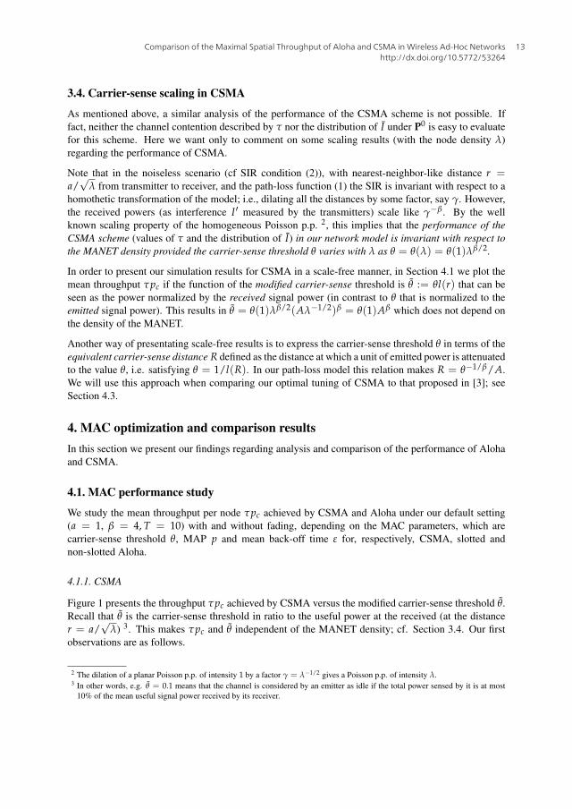
Figure 1 presents the throughput τpc achieved by CSMA versus the modified carrier-sense threshold θ.

Recall that θ is the carrier-sense threshold in ratio to the useful power at the received (at the distance

r = a/√

λ) 3. This makes τpc and θ independent of the MANET density; cf. Section 3.4. Our first

observations are as follows.

2 The dilation of a planar Poisson p.p. of intensity 1 by a factor γ = λ−1/2 gives a Poisson p.p. of intensity λ.3 In other words, e.g. θ = 0.1 means that the channel is considered by an emitter as idle if the total power sensed by it is at most

10% of the mean useful signal power received by its receiver.


13


Remark 4.1. In the absence of fading the maximum throughput of 0.068 (unit-size packets per unit of

time and per node) is attained by CSMA when the carrier-sense threshold is fixed roughly at the level

of θ = θ∗ = 0.08. This optimal tuning of the carrier-sense threshold seems to be quite insensitive to

fading. However, the optimal throughput is significantly reduced by fading. Rayleigh fading of mean

1, reduces the CSMA throughput to 63.2% compared with the no fading scenario.

This latter observation is easy to understand as the channel-sensing is done at the emitter and that fading

at the receiver is independent of fading at the emitter.

0.025

0.03

0.035

0.04

0.045

0.05

0.055

0.06

0.065

0.07

0 0.02 0.04 0.06 0.08 0.1 0.12 0.14 0.16 0.18 0.2

τ p

c

Modified carrier-sense threshold

CSMA

Rayleigh fading no fading

Figure 1. Mean throughput per node τpc versus modified carrier-sense threshold θ in CSMA; Rayleigh fading and no-fadingscenario.

4.1.2. Aloha

Figure 2 presents the throughput τpc with and without fading achieved by slotted Aloha versus the

channel occupation time τ, which in this model is equal to the the MAP parameter p. The results of

non-slotted Aloha are presented in Figure 3 with τ = 1/(1 + ε), where ε is the mean back-off time.

The other parameters are as in the default setting. Here are our observations.

Remark 4.2. In the absence of fading the maximum throughput of 0.028 for the optimal MAP p =p∗ ≈ 0.06. As in CSMA, this optimal tuning seems to be quite insensitive to fading, which in the case

of Rayleigh fading can be evaluated explicitly as p = p∗ = κ−1T−2/β (which gives p∗ = 0.064081

in the default Rayleigh scenario). In contrast to CSMA, Rayleigh fading has a relatively small impact

on the slotted Aloha throughput reducing it only to 92% of the throughput achieved in the no-fading

scenario (in contrast to 63.2% in CSMA). Similar observations hold for non-slotted Aloha, which in the

Rayleigh fading scenario achieves ζ = 2β/(2 + β) = 1.5 times smaller throughput than the slotted

version.

4.2. Impact of model parameters

In Figures 4, 5, 6, 7, 8 and 9 we can study the dependence of the maximal throughput achievable

by the MAC schemes (at their respective optimal tunings) as a function of the path-loss exponent β,



10.5772/53264

0

0.005

0.01

0.015

0.02

0.025

0 0.05 0.1 0.15 0.2

τ p

c

τ

Slotted Aloha

Rayleigh fading - simulationRayleigh fading - model

no fading - simulationno fading - model

Figure 2. Mean throughput per node τpc versus channel occupation τ = p in slotted Aloha; Rayleigh fading and no fading

scenario.

0

0.005

0.01

0.015

0.02

0 0.05 0.1 0.15 0.2

τ p

c

τ

Non slotted Aloha

Rayleigh fading - simulationRayleigh fading - model

no fading - simulation no fading - model

Figure 3. Mean throughput per node τpc versus channel occupation time τ = 1/(1 + ǫ) for non-slotted Aloha; Rayleighfading and no fading scenario.

SIR threshold T and relative distance to the receiver a (recall that a = r√

λ). It is clear that CSMA

significantly outperforms both Aloha protocols for all choices of parameters.

More detailed observations are as follows.

Remark 4.3. The higher path-loss exponent β is, the less advantage there is in using CSMA. When

there is no fading, the increase of β from 3 to 6 reduces the gain in throughput of CSMA with respect

to slotted Aloha from 2.6 to 2.1 and with respect to non-slotted Aloha from 3.5 to 3.2.


15


0.01

0.02

0.03

0.04

0.05

0.06

0.07

0.08

0.09

0.1

0.11

3 3.5 4 4.5 5 5.5 6

τ p c

Path loss exponent β

No fading

slotted Alohanon-slotted Aloha

CSMA

Figure 4. Maximal achievable mean throughput per node τpc versus path-loss exponent β in the absence of fading.

0

0.01

0.02

0.03

0.04

0.05

0.06

0.07

0.08

3 3.5 4 4.5 5 5.5 6

τ p c


Rayleigh fading


CSMA

Figure 5. Maximal achievable mean throughput per node τpc versus path-loss exponent β with Rayleigh fading.

We can also see in Figure 4, that in the absence of fading, slotted Aloha attains the expected fraction of

21% of terminals engaged in successful traffic, foreseen in the seminal paper [9], for SINR threshold

T = 10 and a moderate path loss exponent slightly larger than β = 3.5.

Remark 4.4. The existence of fading (see Figure 5) further diminishes the advantage of CSMA. In

particular, Rayleigh fading reduces the gain in throughput of CSMA with respect to slotted Aloha to

about 1.7 and for non-slotted Aloha to a factor between 2.5 and 2.1 (depending on β).

Studying the impact of the SINR threshold T we observe the following, see Figures 6 and 7.

Remark 4.5. The higher T is (and hence the smaller bit-error rate sustainable in each packet), the

greater is the advantage of using CSMA. In particular, when there is no fading and for β = 4, increasing



10.5772/53264

0

0.02

0.04

0.06

0.08

0.1

0.12

0.14

0.16

0 2 4 6 8 10 12 14 16

τ p

c

Capture threshold T

No fading


CSMA

Figure 6. Maximal achievable mean throughput per node τpc versus SIR threshold T in the absence of fading.

0

0.02

0.04

0.06

0.08

0.1

0.12

0 2 4 6 8 10 12 14 16

τ p

c

Capture threshold T

Rayleigh fading


CSMA

Figure 7. Maximal achievable mean throughput per node τpc versus SIR threshold T. Rayleigh fading.

T from 1 to 11 results in the increase in the gain in throughput of CSMA with respect to slotted Aloha

from 2.4 to 3.5 and this latter ratio remains stable for T larger than 11. For a similar comparison of

CSMA to non-slotted Aloha the gains are from 1.8 to 2.6. In the case of Rayleigh fading the analogous

gain factors of CSMA are, respectively, from 1.8 to 2.4 with respect to slotted Aloha and from 1.4 to

1.8 with respect to non-slotted Aloha.

Finally we study the impact of the relative distance to the receiver a (in ratio to the mean distance to

the nearest neighbor in the network). Figures 8, and 9 show clearly that this distance should be kept as

small as possible without disconnecting the network.


17


0

0.02

0.04

0.06

0.08

0.1

0.12

0.5 1 1.5 2 2.5 3 3.5 4

τ p

c

’a’ relative distance to the receiver

No fading


CSMA

Figure 8. Maximal achievable mean throughput per node τpc versus a the distance transmitter receiver. No fading.

0

0.01

0.02

0.03

0.04

0.05

0.06

0.07

0.5 1 1.5 2 2.5 3 3.5 4

τ p

c

’a’ relative distance to the receiver

Rayleigh fading


CSMA

Figure 9. Maximal achievable mean throughput per node τpc versus a the distance transmitter receiver. Rayleigh fading.

4.3. Optimal tuning of Aloha and CSMA

For Aloha the optimal tuning of τ can be obtained analytically from (7) whereas the optimal tuning

of CSMA is obtained by simulation. In Figure 10, we present the optimal values of τ versus β with

Rayleigh fading for both Aloha and CSMA.

Remark 4.6. We observe that the more sophisticated the MAC scheme is, the more it can content to

the channel when the MAC is tuned optimally. Additionaly the more sophisticated MACs also exhibit

higher capture probabilities. In particular our simulations show the that this probability is close to 1

(between 0.8 and 0.95) for CSMA.



10.5772/53264

A practical conclusion that can be drawn from these observations is that the carrier-sense threshold in

CSMA should be chosen at the largest possible value at which the allowed transmissions are almost

always successful.

0.02

0.04

0.06

0.08

0.1

0.12

0.14

3 3.5 4 4.5 5 5.5 6

τ


Rayleigh fading


CSMA

Figure 10. Optimal value of τ for Aloha and CSMA versus β with Rayleigh fading

4.4. Nelson & Kleinrock’s model of CSMA revisited

Remark 4.6 might explain why the significant superiority of CSMA with respect to Aloha was not

observed in [3]. Let us be more precise and revisit this model.

The simple propagation model in [3] assumes a fixed transmission range R and the same carrier-sense

range. In other words, any two successfully communicating nodes need to be within distance R from

each other and no other transmission should occur in the distance R from the receiver.

In this model, an ideal medium access scheme suggested in [3] should be able to choose from the

given pattern of nodes centers for a maximal number of hard (non-intersecting) disks of radius R. The

asymptotic analysis of the performance of such an ideal scheme is done in [3] assuming an increasing

density of nodes λ. Namely, if this density is large, then the optimal scheme should be able to chose

the pattern of nodes close to the hexagonal packing, known to obtain the densest packing of hard disks

of radius R. Such a packing attains the fraction of 0.90689 of the plane covered by the union of disks.

Consequently, since there is no disk overlapping, it would choose the fraction

τideal =0.90689 × network area

# of nodes × exclusion disk surface area=

0.90689

λπR2

of the nodes of the network, whose density is λ nodes per unit of surface. This expression can

be interpreted as the contention parameter of this ideal medium access scheme, which explains our

notation. Since all transmissions allowed by this scheme are successful, we have pc = 1 for it and the

achieved throughput per node is 0.90689/(λπR2).


19


Regarding CSMA, the simple propagation model with transmission range equal to the carrier-sense

range, assumed in [3], corresponds to a choice of nodes such that any selected node is not covered

by the transmission range of any other selected node. This task is equivalent to the packing of hard

disks of radius R/2. For some reason, that is partially explained in that paper, a slightly larger radius

1.2881R/2 is taken. Similar to the ideal scheme, asymptotic analysis of the hexagonal pattern, gives

the contention parameter of this CSMA scheme equal to

τCSMA =2.214

λπR2.

Moreover, assuming that each authorized node chooses its receiver uniformly within the transmission

range R, and calculating the fraction of the area within this range that is not covered by any other disk

(no collision), the successful transmission probability is calculated as pc = 0.2034. Consequently the

throughput achieved by this CSMA is τpc = 0.4504/(λπR2).

Note that apparently the sub-optimal assumption of the carrier-sense range equal to the transmission

range in the above model of CSMA leads to a relatively small successful transmission probability pc =0.2034, close to that obtained by Aloha, which explains why there is no essential difference between

the performance of these two schemes. Our optimally tuned CSMA model seems to be closer to the

ideal scheme of [3], at least because the probability of successful transmission is much closer to 1.

Let us now try to compare the performance of our optimal CSMA and the two schemes of [3]. This

is not straightforward, since unlike ours, the results of [3] scale in 1/λ are only valid asymptotically,

when λ → ∞ (due to the hexagonal approximation of the perfect packing). However, note that in

the model of [3], the expression N = λπR2 corresponds to the expected number of nodes within

the area contended (blocked) by one given authorized transmission. Consequently the constants ρ =0.90689 = τpc N and ρ = 0.4504 = τpc N can be interpreted, respectively in the two models, as

the expected number of successful transmissions per set of nodes contended (blocked) by one given

authorized transmission. This kind of spatial efficiency can be evaluated in our model using the notion

of the equivalent carrier-sense distance R = θ−1/β/A = rθ−1/β introduced in Section 3.4. Taking

N = λπR2 with R calculated as such we obtain for our CSMA ρ = τpc N = τpcλπr2 θ−2/β. For

the optimally tuned CSMA in the standard scenario a = 1, T = 10, β = 4 without fading we have

ρ = 0.07π0.08−1/2 = 0.77750 of successful transmissions per set of nodes contended (blocked) due

to one given authorized transmission. This is a much better performance than ρ = 0.4504 for CSMA

of [3], and in fact closer to ρ = 0.90689 achieved by the ideal scheme of [3].

4.5. Corrective terms

In this article we have not considered the effect of the back-off for CSMA, and for slotted Aloha we

have ignored the guard times to avoid overlapping of the slots. In this sub-section we briefly study

the effects of these parameters on performance. Let us call δ the ratio of maximum propagation time

plus detection time in the network over the packet transmission time. Back-off in CSMA leads to

wasting time and to collisions for nodes starting their transmissions within the same mini-slot of size

δ× packet transmission time. We know that the reduction of the throughput for CSMA is 1

1+√

2δwhen

the back-off is properly tuned, see [2] chapter 4. For slotted Aloha and with the same assumptions, the

guard times lead to a reduction of approximately 11+δ . Thus for δ = 0.05, 0.02 and 0.01 we obtain a

throughput reduction of respectively 0.76, 0.83, 0.87 for CSMA and 0.95, 0.98, 0.99 for slotted Aloha.

Thus, the throughput reduction is greater for CSMA than for slotted Aloha but these corrective terms

do not change our main observation which gives a notably higher throughput to CSMA.



10.5772/53264

5. Conclusions

In this paper we compare slotted and non-slotted Aloha with CSMA in a Poisson ad-hoc network

setting with SINR-based capture condition. We assume the usual power-law path-loss function and

both Rayleigh and no-fading scenarios. To obtain a fair comparison between these protocols, their

parameters are tuned to achieve the maximum successful transmission rates. Our analysis shows that

CSMA always outperforms both slotted and non-slotted Aloha. However the gain obtained when using

CSMA is slightly reduced by increasing path loss and more significantly by the existence of fading. We

also show how to tune the carrier-sense threshold in CSMA so as to obtain its optimal throughput for an

arbitrary network density. Our models concur with those of [3] even though some results may appear,

at first glance, to be somewhat contradictory, because in [3] CSMA is not optimized.

Author details

B. Blaszczyszyn1,2, P. Mühlethaler1 and S. Banaouas

1 INRIA Paris-Rocquencourt, France

2 ENS Paris, France

References

[1] L. Kleinrock and F. A. Tobagi. Packet switching in radio channels: Part I-Carrier-sense

multiple-access modes and their throughput-delay characteristics. IEEE Trans. Commun., vol.

COM-23, pages 1400–1416, 1975.

[2] D. Bertsekas and R. Gallager. Data Networks. Prentice-Hall, Englewood Cliffs, 2001.

[3] R. Nelson and L. Kleinrock. Maximum probability of successful transmission in a random planar

packet radio network. In Proc. of IEEE INFOCOM, San Diego, April 1983.

[4] F. Baccelli, B. Blaszczyszyn, and P. Mühlethaler. An Aloha Protocol for Multihop Mobile

Wireless Networks. In Proceedings of the Allerton Conference, University of Illinois, Urbana

Champaign, November 2003. also in IEEE Transactions on Information Theory, 52(2):421–436,

2006.

[5] B. Błaszczyszyn and P. Mühlethaler. Stochastic analysis of non-slotted Aloha in wireless ad-hoc

networks. In Proc. of IEEE INFOCOM, San Diego, CA, 2010.

[6] M. Haenggi. Outage, local throughput, and capacity of random wireless networks. IEEE Trans.

Wireless Comm., 8:4350–4359, 2009.

[7] J. Abate and W. Whitt. Numerical inversion of laplace transforms of probability distributions.

ORSA Journal on Computing, 7(1):38–43, 1995.

[8] N. Abramson. The Aloha system - another alternative for computer communication. In Proc. of

AFIPS, pages 295–298, 1970.

[9] R. Nelson and L. Kleinrock. The spatial capacity of a slotted Aloha multi-hop packet radio

network with capture. IEEE Trans. Comm., 32:684–694, 1984.


21


[10] C. Bordenave, S. Foss, and V. Shneer. A random multiple access protocol with spatial interactions.

In Proc. of WiOpt. IEEE, Limassol, Cyprus, 2007.

[11] J. Kim and Leu. Capture Effects of Wireless CSMA/CA/Protocols in Rayleigh and Shadow Fading

Channels. IEEE Transactions on Vehicular Technology, 48:1277–1286, 1999.

[12] R. Boorstyn, A. Kershenbaum, B. Maglaris, and V. Sahin. Throughput analysis in multihop csma

packet networks. In IEEE Transactions on Communications vol. 35, no. 3, pages 267–274, 1987.

[13] José M. Brazio and Fouad A. Tobagi. Theoretical results in throughput analysis of multihop packet

radio networks. In In Proceedings of ICC, pages 448–455, 1984.

[14] M. Garetto, T. Salonidis, and E. Knightly. Modeling per-flow throughput and capturing starvation

in csma multi-hop wireless networks. In IEEE/ACM Transactions on Networking, pages 864–877,

August 2008.

[15] Michele Garetto, Theodoros Salonidis, and Edward W. Knightly. Modeling per-flow throughput

and capturing starvation in CSMA multi-hop wireless networks. In In Proc. of IEEE Infocom,

Barcelona, SPAIN, 2006.

[16] K. Medepalli and F.A. Tobagi. Towards performance modeling of IEEE 802.11 based wireless

networks: A unified framework and its applications. In Proc. of IEEE INFOCOM, Barcelona,

SPAIN, 2006.

[17] Yu Wang and J.J. Garcia Luna-Aceves. Modeling of collision avoidance protocols in

single-channel multihop wireless networks. In Wireless Networks, Volume 10 Issue 5, 2004.

[18] G. Bianchi. Performance analysis of the ieee 802.11 distributed coordination function. In IEEE

Journal on Selected Areas in Communications, volume 18 No.3, pages 535–547, 2000.

[19] Lili Qiu, Yin Zhang, Feng Wang, Mi Kyung Han, and Ratul Mahajan. A general model of wireless

interference. In MOBICOM, pages 171–182, 2007.

[20] Huu Quynh Nguyen, François Baccelli, and Daniel Kofman. A stochastic geometry analysis of

dense ieee 802.11 networks. In INFOCOM, pages 1199–1207, Anchorage, Alaska, 2007.

[21] Mariam Kayna and Nihar Jindal. Performance of Aloha and CSMA in spatially distributed

networks. In ICC, pages 1108–1112, 2008.

[22] European Commission. COST 231. Evolution of land mobile radio (including personnal)

communications. Final report. Information, Technologies and Sciences. Springer, 1999.


intech-aloha and csma in wireless ad hoc networks

Documents