intech-hysteresis modeling of soft magnetic materials using labview

6

Hysteresis Modeling of Soft Magnetic Materials using LabVIEW

Septimiu Motoasca Transilvania University of Brasov

Romania

1. Introduction

This chapter deals with analytical modeling of hysteresis cycle using the powerful mathematical tools from LabVIEW. For magnetic materials one of the most important characteristics is the hysteresis cycle. In numerous technical applications it is necessary to have a mathematical representation of magnetic characteristics in form M = f(H) or B = f(H) in order to calculate magnetic field especially in various rotating machines or electromagnetic apparatus. There are many physical models used for modeling the hysteresis cycle. Many of them are not so easy to implement, require too many data to be introduced or are time consuming. Two models are most used in practice: Preisach model and Jiles-Atherton model. In this chapter is presented the way to realize the program using LabVIEW VI’s for these two models and comparison between the modeled data and measured ones. A new simple analytical model using straight-line segments and arcs of circle to express the hysteresis cycle is also presented. This program for modeling the hysteresis cycle having the smallest amount of input data possible is suitable for soft magnetic materials. The easiness of using this model consists in the fact that it uses only nine parameters as input data, is very quick computed and give a good approximation of the measured hysteresis cycle. There are two variants of the program used for this model one using the LabVIEW VI and MatLab script block and other using only LabVIEW VI’s.

2. Preisach model

2.1 Theoretical aspects of classical Preisach model

In this model, the ferromagnetic material is considered a basic set of fields called elementary

dipoles, Preisach dipoles or Preisach operators. Each dipole is characterized by a rectangular hysteresis cycle and asymmetric [30] (Figure 1). Each dipole can be in any time in a positive saturation state (1) or negative saturation (-1). Transition between states is determined by the magnetic field value H compared with values hof = of, hb = b Field called critical or tipping. If a state of saturation dipole is negative (-1) and the value of H increases above the H = ha = a it toggles the state (1). To return to its original state, the field will be decreased to below H = hb = b (b <a).

www.intechopen.com

Modelling, Programming and Simulations Using LabVIEW™ Software

108

Fig. 1. Elementary Cycle (dipole) Preisach.

The problem to characterize the actual material is finding a statistical distribution of elements according to the values of variables of and b. This distribution is represented in the plane (a, b) and is called the Preisach distribution p(a, b) . With this distribution function is determined the global flux (magnetization), at a time of material. Physical interpretation of the model can be given for weak fields, in agreement with the Neel theory of magnetism that consider that energy of moving Bloch wall has a stepped profile. The idea can be extended to more intense fields, considering the lock-release mechanism walls cvasistationary regime. Some properties of classical Preisach model are listed below: - Property removal: each maximum (respectively minimum) local input size erase all

maxims (respectively minima) above that are lower (respectively higher) value; - Matching property of the minor cycles: minor cycles measured between the same

extreme values of the magnetic field are equaled (congruent); - Symmetry property that results from cyclical developments of H between values -H1

and +H1 produces symmetrical cycles. So symmetrical cycles obtained are one inside another, with no intersections.

Subsequent studies led to the conclusion that removal properties and the matching is necessary and sufficient conditions for a hysteretic system are properly represented by the classical Preisach model. Must be mentioned the limitations imposed by this model, which means, eventually, an approximation of a real phenomenon: - Model is static, not taking into account how variables change over time. The model

need only the extremes of input size; - Reversible magnetization phenomena are not taken into account; - Phenomenon of habituation is ignored; reptation phenomenon of minor cycles is not

modeled, closing cycles are minor points well established as the clear property.

www.intechopen.com


109

For calculation of magnetic induction or magnetization is using the formula:

( )( ) ( , ) ,B t p a b sign m a b dadb⎡ ⎤= ⋅ ⎣ ⎦∫∫ (1)

where: p(a, b) represent the Preisach function which will be represented as a triangle in the space (a, b) sign[m(a, b)] is the sign of Preisach elementary operator m(a, b). This operator changes sign in concordance with the magnetic field strength variation. The identification operation for classical Preisach model involves determining the distribution function of the dipole unitary p(a, b). For this goal it can be proceed in two ways: - Search function is divided in small rectangles of points (ai, bj) like a mesh and in each

rectangle a value p(ai, bj) is inserted resulting from the experimental data; - Is assumed to known an analytical form of function (eg. Gaussian distribution) and

identified based on measurements only the needed function parameters. For determining a mesh function p(ai,bj) based on experimental data, two main methods are known: - Biorci method [9] (requires 3N points for determining probabilities: the 1N from first

magnetization curve and 2N on the descending major hysteresis cycle unless the cycle is considered symmetric, otherwise requires 5N points and additionally are needed another 2N points on the ascending branch of a major hysteresis cycle).

- Mayergoyz method (method requires more experimental data than the method Biorci ( 2N2 instead of 3N ), but accuracy is improved).

2.2 LabVIEW program using Preisach model

As previously mentioned, modeling hysteresis cycles were done using LabVIEW program, given the possibility of modular programming, using scripts in MatLab, obtaining handy charts and ported to other applications and the possibility to change inputs in real-time when program run continuously. The full program is presented in Annex 1. The first step in modeling program using Preisach hysteresis cycle was to make a triangle in the Preisach space (a, b) which have a predefined number of points and create some Preisach function (also called weights) in each cell (ai, bj), respecting model properties listed above . For this step, the block presented in Figure 2 was done, using the LabVIEW programming environment, in the block diagram. At the end of this block is obtainded a Preisach triangle with a simple analytical form of distribution so as to obtain symmetrical distribution of weighting point’s ai, b j.

Fig. 2. Block performing Preisach triangle.

www.intechopen.com


110

In this block , two cycles for was used to create space (ai,bj) , and in each element of the cell is introduced an analytical value of the Preisach function. The result of this block may be highlighted on a chart is shown in Figure 3. This analytical model was made only as a demonstration but the analytical form which must be inserted in each cell need much more calculations for real case tacking account of great number of data needed as input which must be inserted manual in each cell. In figure 3, it can be seen Preisach distribution weights for N=100 points and arrangement according to two variables a andr b. It can be observed that is respected the principle of symmetry that is set for the Preisach model. Next step that should be done is tilted fields according to an incremental or decremented change as a input function corresponding change in magnetic field strength H of a certain shape.

Fig. 3. Preisach triangle obtained at the exit of the first block.

For example, I used a saw-tooth function in which the amplitude is reduced to simulate the phenomenon of demagnetization. Function used as entry can be of another form (eg. sinusoid). It also may be introduced from an external file, like the change of the shape of a magnetic field strength as experimentally measured.

Fig. 4. Shape variation of the magnetic field intensity H.

For this case, the function used is shown in Figure 4, it was highlighted on a chart obtained from the LabVIEW environment. This function was created using LabVIEW environment by introducing the function values in a column matrix.

www.intechopen.com


111

This waveform obtained is used as input in a block, shown in Figure 5, which carries out basic fields tilted to plus to minus and vice versa depending on the passage above a certain value of H. Also on that block entry is placed the previously obtained Preisach triangle.

Fig. 5. Block tilting elementary Preisach domain.

This block has three loops for in which the Preisach triangle is decomposed in each elementary area. The first loop's is for H input waveform decomposition in the values for each step of time and is designed to save the final after making Preisach triangle areas in other two loops for.

Fig. 6. Demagnetization triangle after having gone through the entire cycle.

In the first loop for was introduced a timer which makes the program to run in a given time to be able to see in the graphs in front panel the application of tilted fields on Preisach

www.intechopen.com


112

Triangle. Preisach triangle undergoes changes during each step and the final position can be seen on a graph shown in Figure 6. The other two loops for are used for the Preisach triangle decomposition in elements and the value of each element is tilted from plus to minus or vice versa taking into account the variation of input waveform. Using the results obtained from this block and summing Preisach elements is obtained a waveform for magnetic induction or magnetization. Introducing the waveform of Magnetic field and obtained waveform for magnetic induction as input to a XYgraph is obtained the hysteresis cycle shown in Figure 7.

Fig. 7. Hysteresis cycle obtained using the program developed in LabVIEW .

The most difficult part of the Preisach model is the calculation of Preisach elementary functions (weights). In our theoretical model we not used the experimental data because is very difficult to calculate and populate the triangle considering 300 points on first magnetization curve and descending branch of hysterezis cycle. We tried several options for calculating the weighting coefficients using analytical methods but the appearing equations are very difficult to solve for experimental data. Therefore, we made another Preisach modeling program that has as input the experimental measured values and weights were calculated using only the descending branch of the major hysteresis cycle considering that is a symmetrical cycle. This program is presented in the next subchapter, the method of calculating the weights being a personal contribution to this model. It can be concluded that this model is quite easy to implement but requires finding a large weighting calculation and correlation with experimental data. The Preisach analytical functions that calculate weights can not give a sufficiently good approximation for the model. The full program is presented in Annex 2.

2.3 Modified Preisach method

To calculate the weights have been proposed several methods [4], [7], [15], [35], [38], [65]-[72]. In this chapter, is presented a method for calculating weights using only the descending branch of the major hysteresis cycle. For this case, first builds a Preisach triangle that initially will have only half the amount of space populated with + 1 value and 0 otherwise.

www.intechopen.com


113

Fig. 8. Making Preisach triangle.

This first triangle will be changed in a block shown in Figure 9. As input for this block is used the triangle made in the block shown in Figure 8 and measured data values for the descending branch of major hysteresis cycle. Before making the calculation of the weights of Preisach triangle, was an interpolation of experimental data for descending branch of hysteresis cycle so that the number of experimental data to correspond to the value of the n points chosen to achieve Preisach triangle.

Fig. 9. Calculating the weights of block cells Preisach triangle .

Operation is performed for calculating the weights in n steps. Using data for the magnetic flux density was measured dividing the weights so that each step is calculated weights for a whole range of values of hb and all possible values of ha. Considering that the hysteresis cycle is symmetric around the origin can be considered the same values and ascending branch of a major hysteresis cycle. To first step considered in the first cell is obtained by subtracting the value derived from the saturation value (Bs = B0) the following item (B1) on the downward curve. The rest of the remaining cells, the total amount will be B1. In the next step, the first cell remain as previously calculated. Cells of the next line (hb = ct.) for the next step will be the total value B1-B2 and the remaining cells are considered the overall value B2. This reasoning is repeated until reaching a negative saturation value.

www.intechopen.com


114

By reversing these values are inserted upward branch of the same values and thus succeeded in dividing each line (hb = ct.) component weights in their cells, taking into account the ascending branch. The block in Figure 10 is tilted out of the cells for varying Preisach triangle field obtained in this case the measured values.

Fig. 10. Preisach triangle block tilting for varying magnetic field strength .

For example, were used as input values measured using the DC to determine first order return curves . Figure 11a is shown as the variation of the magnetic field and in Figure 11b , is shown as the variation of magnetic induction measured .

Fig. 11a. Shape variation of the magnetic field intensity.

www.intechopen.com


115

Fig. 11b. Shape variation of magnetic induction measured.

Fig. 11c. Hysteresis cycle obtained from measured data.

In Figure 11c is shown the hysteresis cycle as obtained from measured data. In Figure 12 is presented the modeling results using this method for calculating the weighting Preisach.

www.intechopen.com


116

Fig. 12. Cycle Preisach modeling method using the computer program presented

For better illustration, in Figure 13, 3D representation was achieved resulting Preisach triangle.

Fig. 13. 3D representation of the Preisach triangle

It appear that the modeling approach may not exactly follow the measured curve but if is choose more points for Preisach triangle the modeling cycle will be closer to the experimentally obtained one. It should be noted that the Preisach method is evident shortcomings in this case, some places having predetermined cycle end which cannot follow the experimental measurements.

www.intechopen.com


117

This way of modeling is good for a fairly large number of entry points. This shortcoming can be overcome using software interpolation between the points and we obtain the descending branch. Interpolation method also introduces its errors in the program. Very small variations around a value, as is apparent in our case around positive saturation will stop all at the same point. Full program in block diagram and the front panel results are presented in Annex 3.

3. Jiles - Atherton model

3.1 Langevin model his eyesis the paramagnetism

The first microscopic model of magnetic materials was presented by Langevin. He takes m total magnetic moment moment of an atom including spin and orbital moment of movement . If the magnetic field strength H, then the potential energy is calculated using the formula:

0 0 cosmw mHμ μ= − = − ΘmH (2)

where: Θ is the angle made between vectors: magnetization and applied magnetic field strength. Langevin assumed that the atomic magnetic moments m in paramagnetic materials do not interact. Using the classical Maxwell-Boltzmann statistical probability that an atom to have energy wm has the expression:

( ) mw

kTmp w e

−= (3)

where : - k = 1.381 10-23 J / K is Boltzmann's constant and - T is absolute temperature. When the electric field intensity vector will have the same direction as magnetization vector can talk about inner model describing the relationship between these two sizes. If the directions of the two components differ then be considered a model vector. Eddy current losses are dependent by the frequency excitation field and are not negligible. If these addition losses and other types of losses may be neglected then the proposed model can be a model independent of frequency.

3.2 Theoretical aspects on Jiles - Atherton model

Model proposed by Jiles and Atherton in 1983 presents a series of equations to determine the magnetization of ferromagnetic materials taking into account the principles of physics. After this the model has been continually improved by other authors. This model is widely used to achieve hysteresis cycles and required to calculate or identify only five parameters. It seems that this way of identifying the parameters is the great shortcoming of this method. Tried to identify parameters based on measured data is not so easy at it seems. Ideal is to find a mathematical system to calculate the parameters in order to obtain a minimum error between measured and simulated curves. The Jiles - Atherton model are the two mechanisms underlying the magnetization: - domain wall displacement; - growth areas in the direction of the magnetic field is applied against those who are

pointing in other directions .

www.intechopen.com


118

In the Jiles - Atherton model the magnetization is composed of two terms: reversible magnetization and irreversible magnetization.

irr rev= +M M M (4)

The irreversible component is given by the irreversible movement of domain walls. Magnetizaţia reverse is reversible once the growth areas. Hysteresis cycle can be drawn based on the equilibrium energy density within the material.

mag hysw w w= + (5)

Energy density which is generated by the irreversible movement of domain walls can be calculated using the formula:

0 irrdw kdMμ= (6)

where: k - is a pinning factor. Ferromagnetic materials interact in neighboring areas, so it is introduced the concept of effective magnetic fields acting on unit volume. Consequently, the magnetization will be regarded as a function of magnetic field strength actually considering moving energy loss generated by irreversible domain wall:

0irr

bloh e

e

dMdw k dH

dHμ δ= (7)

where: ( / )esign dH dtδ = .

Modification of irreversible magnetization can be obtained from the calculation of energy. Energy consumed by the material is divided into two parts: the exchange energy and energy loss through hysteresis.

0 0 0( ) ( )an

dMM H dH M H dH k dH

dHμ μ μ δ= +∫ ∫ ∫ (8)

hence:

( ) ( )an

dMM H M H k

dHδ= + (9)

If during the process of magnetization, the anhisteretic magnetization has values lower than this leads to a solution for irreversible magnetization physically impossible, as if the domain walls can not move. Solution of differential equation is:

1

( )

0

an irr e an irrirr

an irr

M M dH if M MdM k

if M Mδ

⎧ − >⎪= ⎨⎪ <⎩ (10)

Reverse magnetization may be taken into account by introducing the coefficient c. which defines the equation as:

( )rev an irrM c M M= − (11)

www.intechopen.com


119

Hence the total magnetization became:

(1 )an irrM cM c M= + − (12)

If its value is inserted M the differential equation is obtained

1

( )an irr e an an irr

an an irr

cM M dH cdM if M M

dM kcdM if M M

δ−⎧ − + >⎪= ⎨⎪ <⎩

(13)

Each step can be determined from the previous value of the magnetization using formula:

1

1( )an j e an an irr

j

an an irr

M M dH cdM if M MdM k

cdM if M Mδ+

⎧ − + >⎪= ⎨⎪ <⎩ (14)

This formula is used for numerical implementation of the model proposed by Jiles and Atherton. In the literature [56]-[59], [89], [93], are proposed several methods of identification of parameters but it seems that no procedure is too easy, requiring input rather difficult and experimental features. To determine the values of input parameters need to know more points on the hysteresis cycles obtained by experimentally means: - coercive magnetic field strength (Hc) ; - remnant magnetization (Mr) ; - saturation coordinates (Hs, Ms) ; - susceptibility in coercitivity point - susceptibility at point of remanance - susceptibility at the saturation point - anhisteretic susceptibility - initial susceptibility - maximum susceptibility Parameter identification procedure based on these initial data is described in [15]. There is an easy procedure and therefore no result is as expected, the cycle obtained with large deviations from the shape obtained experimentally. For this reason we opted for a process for identifying the parameters by calculating the error between the curves obtained experimentally and modeled by the method of Jiles - Atherton.

3.3 LabVIEW modelling program using the Jiles - Atherton model

Jiles-Atherton model was implemented using LabVIEW programming environment for the reasons listed before. In figure 14 is presented in the LabVIEW program. As can be observed in Figure 14 the model was implemented in a cycle for to make the calculation of magnetization in each step, and can implement equations (14) for recurrence. Magnetic field intensity values can be obtained using a generator as a sine wave or taking data from a file containing the actual measured values, which are find using block for retrieving data from files from virtual instruments and accessing the PATH of the file. To calculate total magnetization the cycle must be brought to saturation point. It is obtained from measured data or can be inserted in a parameter input box Bs from front panel of the program.

www.intechopen.com


120

Fig. 14. Block diagram of LabVIEW program for modeling Jiles-Atherton.

www.intechopen.com


121

Fig. 15. The front panel of LabVIEW program for modeling Jiles - Atherton .

In figure 15 are presented the waveforms for H and M and hysteresis cycle as a graphic M(H). To give validity to the model this was compared with measured data and a program to minimize errors between modeled and measured cycle was proposed. This program is presented in Annex 4.

4. Analytical-geometric model

4.1 Theoretical aspects of analytical-geometric modeling

According to the Nicolaide model presented in [68]-[70], the major hysteresis cycle can be modeled using arcs of circle and straight-line segments in a satisfactory manner. To achieve the design it must be made several simplifying assumptions on the hysteresis cycle like the hysteresis cycle is considered symmetrical and centered at the origin. In the present study taking into account the special characteristics of soft magnetic materials, we have adapted the method from [68]-[70] to studied case and obtain a much more simplified model requiring a small amount of input data. Based on these simplifying assumptions one can construct a cycle branches, other details are obtained automatically by reversing field and magnetic induction or magnetization values, depending on the cycle shape. As can be seen in Figure 16, for modeling downward branch is necessary to know some reference points as follows: 1. saturation point in quadrant I, characterized by the magnetic field saturation value HS

and magnetic induction BS and slope tangent to the cycle at this point; 2. point 2 between two arcs , characterized by values H2 and B2;

www.intechopen.com


122

3. remnant induction Br (which implicitly means that Hr = 0); 4. coercive magnetic field strength Hc (which implicitly means that Bc = 0); 5. coordinates of point 5 where the loop starts tilting cycle (which will be calculated); 6. coordonates of point 6 at joint of two arcs characterized by coordinates H6, B6; 7. negative saturation point, characterized by -HS-BS. In addition to work [84]-[86] where was used 11 parameters we considered that under appropriate conditions for soft magnetic materials, some of these parameters can be obtained from other conditions, and we restrict the number of parameters to only nine. These parameters are: HS, BS, nS (slope of the tangent at the point of saturation) H2, B2, Br, Hc, H6, B6. Accurate representation is given on how to choose the coordinates of points 2 (H2, B2) and 6 (H6, B6). We try to develop a program to change the position of point 2 and 6 in order to have the smallest error between the cycle of measured and modeled in this way.

Fig. 16. Considered reference points for modeling hysteresis cycle

In Figure 16 is shown that between point 1 and point 2 is traced an arc of circle which is tangent to the point (HS, BS), tangent slope is known ns and passing through point 2, whose coordinates are known (H2, B2). Finally knowing the arc of a circle can be calculated from the slope of the tangent to the arc of a circle in section 2. Between point 2 and point 3 is plotted a different arc. The slope of the tangent point 3 is calculated using the coordinates of two points 3(0, Br) and 4(Hc, 0). 2-3 arc is tangent to the slopes calculated previously in arc 1-2 and to straight-line segment 3-4. Between 3 and 5 point is a straight-line segment passing through 4 and has previously calculated slope with points 3 and 4. Coordinates resulting from the calculations forc arc 5-6 as the date of the intersection points between straight line which passes from points 3 and 4 and intersect the arc 5-6 in point 5. For this reason the point 5 is obtained intersecting a circle

H [ A / m ]

B [ T ]

www.intechopen.com


123

obtained from point 6 which must be tangent to the slope in point 6 and to the straight line determined by point 3 and 4. In the arc 6-7 is calculate the slope in point 6 as in case in which is calculated in point 2. Coordinates of point 7 is obtained taking into account the symmetry condition. Linking the arcs and straight-line segment we obtain the descending branch and using an inversion technic taking into account the symmetry principle is btained the ascending branch of hysteresis cycle.

4.2 LabVIEW program for modeling hysteresis cycle

Figure 17 is shown modeling program using LabVIEW software. For solving analytical equations of circular arcs and straight segments, we used a MatLab script window. LabVIEW program was used because of its flexibility to integrate scripts in MatLab and the ease with which experimental data can be stored in text files. It is noted that block entry into MatLab scripts are 10 input parameters of the nine parameters are input parameters above and the tenth is a step that gives the number of points needed for representation.

Fig. 17. LabVIEW program wish to use analytical modeling by arcs and line segments .

To see how well the program approximates the experimental data was achieved overlap values obtained by modeling with experimental values stored in text file in the location given by the block "path". The result of this representation can be seen in Figure 18. As can be seen in the window each spring MatLab script was treated separately and has developed a sampling interval between two field values considered for early and late spring using variable step introduced by the operator as input parameter. Using this step each spring is obtained by a column matrix for magnetic field strength and magnetic induction value. These matrices are concatenated, achieving one matrix with different values of magnetic field strength magnetic flux density values. Using these two matrix representation can be achieved descending branch of the hysteresis cycle.

www.intechopen.com


124

To obtain the upward branch of the hysteresis cycle is made denying the two columns values obtained previously, given the condition of symmetry and centering the zero major hysteresis cycle. Resulting cycle is shown in Figure 18. For comparison, measured using a cycle using the Epstein and installation of measurement in Brockhauss Messtechnik. This measurement cycle was extracted from an excel file obtained by exporting data from MPG program. The program, using the call block file path and measured data are collected and induction magnetic field strength values and shown on the same graph shown in Figure 51. It should be noted that the two cycles overlap quite well in the saturation, with sharp differences in the curves around May remanence. These errors can be minimized if they choose the optimized values of point 2 and 6 but the difference would be too small to be seen.

Fig. 18. Comparison between modeled and the hysteresis curve obtained experimentally .

Improvements are possible by introducing a modeling program to calculate the error function and place most convenient choice for points 2 and 6 so that the error between modeled and actual cycle does not exceed a certain value. To achieve the return cycle of orders 1 and 2 were used repezentare auxiliary functions. Program used for these representations is given in Annex 5. It may be noted that the program to achieve major hysteresis cycle remained the same. In addition to this program were also made blocks MatLab script that calculates the return of the first order curves upward and downward. For easy use, I used buttons for choosing points that reversing the upward branch downward. In this way can choose any point on these branches. In the event that they want certain points, well defined, these buttons can be replaced by dialog boxes for entering a numerical exact values. Full program and graphics on the front panel are presented in Annex 5.

5. Acknowledgement

This paper is supported by The National University Research Council of Romania (CNCSIS) under the contract number 848/2009

www.intechopen.com


125

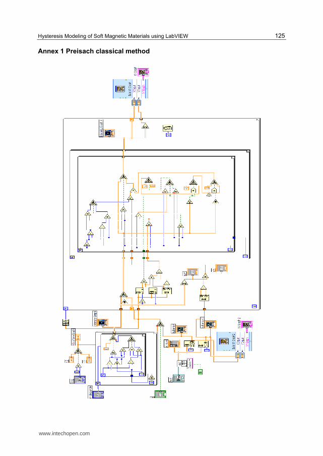
Annex 1 Preisach classical method

www.intechopen.com


126

www.intechopen.com


127

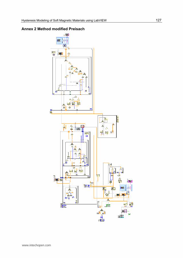
Annex 2 Method modified Preisach

www.intechopen.com


128

www.intechopen.com


129

Annex 3 Method Jiles - Atherton

www.intechopen.com


130

www.intechopen.com


131

Annex 4 Analytic-geometric method

www.intechopen.com


132

www.intechopen.com


133

6. References

[1] FMEA, A., M., Mirmiran, A., A New Model for Steel Members hysteresisInternational Journal for Numerical Methods in Engineering , No. 45 , 1999 , pp 1007-1023 .

[2] Andrew, P., Stancu, A., Adedoyin, A., Modeling of Viscosity Phenomena in Models of hysteresis With Local Memory, Journal of Optoelectronics and Advanced Materials vol 8 , no. March , 2006 , pp 988-990 .

[3] Bennett , L. , H. , Vajda F , Atzmony , U. , Swartzendruber , L. J. Accommodation Study of the Nanograin Iron PowderIEEE Transactions on Magnetics , 32 ( 5 ) , 1996 , pp 4493-4495 .

[4] Bertotti , G. Dynamic generalization of the scalar Preisach model of hysteresis, IEEE Trans . Magna . , No. 28 , 1992 , pp 2599-2601 .

[5] Bertotti , G. General Properties of Power Losses in Soft Ferromagnetic Materials, IEEE Trans . Magna . , No. 24 , 1988 , pp 621-630 .

[6] Bertotti , G. Hysteresis in Magnetism. Academic Press , Inc. . , 1998 California, USA. [7] Bertotti , G. , Basso , V. Pasquale , M. , Application of the Preisach Model to the Calculation of

Magnetization Curves and Power Losses in Ferromagnetic Materials, IEEE Trans . Magna . , No. 30 , 1994 pp 1052-1057 .

[8] Bertotti , G. Fiorillo , F. , Pasquale , M. , Measurement and Prediction of Dynamic Loop Shapes and Power Losses in Soft Magnetic Materials, IEEE Trans . Magna . , No. 29 , March , 1993 , pp 3496-3498 .

[9] Biorci , G. Pescetti , D. Some Remarks on hysteresisJ. Appl . Phys . , No. 37 , 1966 , pp 1313-1317 .

[10] Bossavit , A. Computational Electromagnetism, Academic Press , 1998 Boston. [11] Bottauscio , O. , Chiampi , M. , Chiarabaglio , D. Advanced Model of Laminated Cores for

Two -Dimensional Magnetic Field Analysis, IEEE Trans . Magna . , No. 36 , 2000 , pp 561-573 .

[12] Bottauscio , O. , Chiampi , M. , Chiarabaglio , D. , Raguso , C. , Repeto , M. Ferromagnetic hysteresis and Magnetic Field Analysis, ICS Newsletter , No. 6 , 1999 , pp 3-7 .

[13] Bottauscio , O. , Chiampi , M. , Chiarabaglio , D. , Repetto , M. , Preisach -type hysteresis in Magnetic Field Computation Models, Physica B : Condensed Matter , No. 275 , 2000 , pp 34-39 .

[14] Bottauscio , O. , Chiampi , M. Laminated Core Modeling under Rotational Excitations Including Eddy currents and hysteresisJ. Appl . Phys . , No. 89 , 2001 , pp 6728-6730 .

[15] Bottauscio , O. , Chiarabaglio , D. Chiampi , M. , Repetto , M. , A Periodic Magnetic Field Solution Using Hysteretic Preisach Model and Fixed -Point Technique, IEEE Trans . Magna . , No. 31 , 1995 , pp 3548-3550 .

[16] Bozorth , R. , M. Ferromagnetism. D. Van Nostrand Co. . Inc. . Princeton, 1951 New Jersey.

[17] Burzo , E. Physics of Magnetic Phenomena, Romanian Academy Publishing House , Vol 1 , 1979 , Bucharestknow .

[18] Cardelli , E. Della Torre , E. , Faba , A. Experimental Verification of the deletion and Congruency Property in Si- Fe Magnetic Steels, Modeling hysteresis and Micromagnetics 2009 , some , Gaithersburg , Maryland, USA

[19] Cardelli , E. Della Torre , E. , Faba , A. Properties of a Class of Vector HysteronsJournal of Applied Physics , No. 103 , 2008 , 07D927 .

www.intechopen.com


134

[20] Cardelli , E. , Faba , A. Vector hysteresis Measurements via Single Disk Tester, Physica B , No. 372 , 2006 , pp 143-146 .

[21] Cheng , K. , W. , E. Lu , Y. , Ho , S. , L. Hysteresis Modeling of Magnetic Devices Using Dipole DistributionIEEE Transactions on Magnetics , Vol 41 , No. 5 , 2005 .

[22] Chiampi , M. , Chiarabaglio , D. , Repetto , M. , The Jiles - Atherton and Combined Fixed -Point Technique for Time Periodic Magnetic Field Problems With hysteresis, IEEE Trans . Magna . , No. 31 , 1995 , pp 4306-4311 .

[23] Del Moral Hernandez , E. Muranaka , C. , S. , Cardoso , J. , R. , Identification of the Jiles - Atherton Model Parameters Using Random and deterministic Searches, Physica B 275 , 2000 , pp 212-215 .

[24] Del Vecchio , R. , An Efficient Procedure without hysteresis Modeling Complex Processes in Ferromagnetic Materials, IEEE Trans . Magna . , No. 16 , 1980 , pp 809-811 .

[25] Del Vecchio , R. , Computation of Losses in Electrical Steels Nonoriented From the Classical ViewpointJ. Appl . Phys . , No. 53 , 1982 , pp 8281-8286 .

[26] Del Vecchio , R. , The Inclusion of hysteresis Processes in the Special Class of Electromagnetic Finite element calculations, IEEE Trans . Magna . , No. 18 , ( 1982c ) , pp 275-284 .

[27] Della Torre , E. A Preisach Model for Accommodation, IEEE Trans . Magna . , No. 30 , 1994 , pp 2701-2707 .

[28] Della Torre , E. A Simplified Vector Preisach Model, IEEE Trans . Magna., No. 34 , 1998 , pp 495-501 .

[29] Della Torre , E. Hysteresis Modeling II : Accommodation, IEEE Trans . Magna . , No. 23 , 1987 , pp 2823-2827 .

[30] Della Torre , E. Magnetic hysteresis, IEEE Press, New York , 1999 [31] Della Torre , E. , Pinzaglia , E. Cardelli , E. Vector Modeling - Part I : Generalized hysteresis

model, Physica B , Vol 372 , 2006 , pp 111-114 . [32] Della Torre , E. , Pinzaglia , E. Cardelli , E. Vector Modeling - Part II: Ellipsoidal vector

hysteresis model . Numerical Application to the 2 - D Houses, Physica Male , Vol 372 , 2006 , pp 115-119 .

[33] Dlala , E. Arkkio , A. Measurement and Analysis of hysteresis of High-Speed Torque on Induction Machine, Electric Power Applications, EIT , Vol 1 , No. 5 , 2007 , pp 737-742 .

[34] Dlala , E. Belahcen , A. , Arkkio , A. Vector Model of Ferromagnetic hysteresis Magnetodynamic Steel Laminations, Physica B : Condensed Matter , Vol 403 , No. 2-3 , 2008 , pp 428-432 .

[35] Dlala , E. , Saitz , J. , Arkkio , A. Inverted and Forward Preisach Models for Numerical Analysis of Electromagnetic Field ProblemsIEEE Transactions on Magnetics , Vol 42 , No. 8 , 2006 , pp 1963-1973 .

[36] Dlala , E. , Saitz , J. , Arkkio , A. Modeling Based on Symmetric hysteresis Minor LoopsIEEE Transactions on Magnetics , Vol 41 , No. 8 , 2005 , pp 2343-2348 .

[37] Doong , T. , Mayergoyz , I. , D. Implementation of hysteresis on Numerical ModelsIEEE Transactions on Magnetics , Vol 21 , No. 5 , 1985 , pp.1853 - 1855 .

[38] Fuzi , J. Depends hysteresis model computationally Efficient Rate, COMPEL , No. 18 , 1999 , pp 445-457 .

[39] Fuzi , J. , Helerea , E. Iványi , A. Experimental Construction of Preisach Models for Ferromagnetic Cores, PCIM / PQ , Nuremberg , 1998 .

www.intechopen.com


135

[40] Fuzi , J. Ivanyi , A. Two features of hysteresis Rate - Dependent Models, Physica B : Condensed Matter, No. 306 , 2001 , pp 278-280 .

[41] Fuzi , J. , Kadar , G. Frequency Dependence in the Product Preisach ModelJ. Magna . Magna . Mater . , No. 254-255 , 2003 , p. 278-280 .

[42] Fuzi , J. Type Vector Preisach hysteresis Two Models, Physica B , No. 343 , 2004 , pp 159-163 .

[43] Hantila , F. A Method of Solving Stationary Magnetic Field in Non - Linear Media, rev. Roum . Sci . Techn. - Electrotechn . et Go. , No. 20 , 1975 , pp 397-407 .

[44] Hantila , F. Mathematical Models of the Relation Between B and H for non-linear media, rev. Roum . Sci . Techn. - Electrotechn . et Go. , No. 19 , 1974 , pp 429-448 .

[45] Hantila , F. , Preda , G. , Vasiliu , M. Polarization Method for Static Fields, IEEE Trans . Magna . , No. 36 , 2000 , pp 672-675 .

[46] Helerea , E. , electrical materialsÃ and electronics , Ed MatrixRom , Bucharest , 2003 [47] Henze , O. , Rucker , W. , M. Identification procedures of Preisach model, IEEE Transactions

on Magnetics , Vol 38 , No. 2 , 2002 , pp 833-836 . [48] Henze , O. , Rucker , W. , M. , Jesenik , M. , Gorican , V. , Trlep , M. , Hamler , A. ,

Stumberger , B. , Hysteresis model and Examples of Ferromagnetic Material, IEEE Trans . Magna . , Vol 39 , No. 3 , 2003 , pp 1151-1154 .

[49] Hutchinson , W. , B. , Swift , J. G. Anisotropy in Some Soft Magnetic MaterialsGordon and Breach Science Publishers Ltd. , Texture , Vol 1 , 1972 , pp 117-123 , UK .

[50] Ionita , A. , D. Ionita , V. Software Tools for interoperable between Materials with Electromagnetic Problems involving hysteresis, Proc . of twond Int . Conf on Advances and Applications of GID , 2004 , pp.147 -150 .

[51] Ionita , V , Ionita , A. , D. Use of Magnetic Material Models in Electromagnetic CADJournal of Optoelectronics and Advanced Materials Vol 6 , No. 3 , 2004 , pp 1013-1016 .

[52] Ionita , V. , Crânganu - Cretu , B. , John D. Quasi - Stationary Magnetic Field Computation in Hysteretic Media, IEEE Trans . On Magnetics , Vol 32 , No. 3 , 1996 , pp 1128-1131 .

[53] Ionita , V. , Crânganu - Cretu , B. , Ionita , A. , D. Object- Oriented Software for Advanced Characterization of Magnetic Materials, IEEE Trans . on Magnetics , Vol 38 , No. 2 , 2002 , pp 1101-1104 .

[54] Iványi , A. Hysteresis Models in Electromagnetic Computation, Akademia Kiadó , Budapest , 1997 .

[55] Jiles , D. C. A Generalized Self Consistent Model For The Calculation of Minor Loop in The Theory of Hysterezis ExcursionIEEE Transaction on Magnetics , Vol 28 , 1992 , pp 2602-2604 .

[56] Jiles , D. , C. Atherton , D. L. Ferromagnetic HysterezisIEEE Transaction on Magnetics , Vol 19 , 1983 , pp 2183-2189 .

[57] Jiles , D. , C. Atherton , D. L. Theory of Ferromagnetic HysterezisJournal of Magnetism and Magnetic Materials , Vol 61 , 1986 pp 48-60 .

[58] Jiles , D. , C. Thoelke , J. , B. , Devine , M. , Numerical Determination of hysteresis Parameters for the Modeling of Magnetic Properties Using the Theory of Ferromagnetic hysteresis, IEEE Trans on Magnetics , Vol 28 , No. 1 , 1992 , pp 27-35 .

[59] Jiles , D. , C. Thoelke , J. B. , Theory of Ferromagnetic Hysterezis : Determination of Model Parameters from Experimental hysteresis Loops, IEEE Trans on Magneticws , vol 25 , no. May , 1989 , pp 3928-3930 .

www.intechopen.com


136

[60] Kis , P. , Iványi , A. Parameter Identification of Jiles - Atherton Model With Non - Linear Least -Square Method, Physica B , Vol 343 , 2004 , pp 59-64 .

[61] Kis , P. , Kuczmann , M. , Füzi , J. Iványi , A. Hysteresis Measurements in LabVIEW, Physica B , Vol 343 , 2004 , pp 357-363 .

[62] Krejc , P. , Vector hysteresis Models, Eur . Jnl . Appl . Math . , Vol 2 , 1991 , pp 281-292 . [63] Kuczmann , M. Scalar hysteresis Measurement Using FFTJournal of Optoelectronics and

Advanced Materials , Vol 10 , No. 7 , 2008 , pp 1828-1833 . [64] Lavers , J. , D. , Biringer , P. , P. , Hollitscher , H. A Simple Method for Estimating the Minor

Loop hysteresis Loss in Thin Laminations, IEEE Trans . Magna ., vol 14 , 1978 , pp 386-388 .

[65] Lavers , J. , D. , Biringer , P. , P. , Hollitscher , H. Estimation of Core Loss When the flow waveform Contains the Essential Plus single Odd Harmonic Component, IEEE Trans . Magna ., vol 13 .

[66] Lin , D. Zhou , P. , Badics , Z. , Fu , W. , N. , Chen , Q. , M. , Cendes , Z. , J. A New Model for nonlinear anisotropic Soft Magnetic Materials, Proceedings of COMPUMAG , 2005 , CSY0084 .

[67] Makaveev, D., Dupre, L., De Wulf, M., Melkebeek, J., Combined Preisach–Mayergoyz-Neural-Network Vector Hysteresis Model for Electrical Steel Sheets, Journal of Applied Physics, Vol. 93, No. 10, 2003, pp. 6738-6740.

[68] Nicolaide, A., Magnetism and Magnetic Materials, Transilvania University Press, Brasov, Romania, 2001.

[69] Nicolaide, A., A New Approach of Mathematical Modelling of Hysteresis Curves of Magnetic Materials, Rev. Roum. Sci. Techn. – Electrotechn. Et Energ., Vol. 48, No. 2-3, 2003, pp. 221-233.

[70] Nicolaide, A., An Approach to the Mathematical Modelling of the Hysteresis Curves of Magnetic Materials: The Mirror Curves, Rev. Roum. Sci. Techn. – Electrotechn. Et Energ., Vol. 52, No. 3, 2007, pp. 301-310.

www.intechopen.com

Modeling, Programming and Simulations Using LabVIEW™SoftwareEdited by Dr Riccardo De Asmundis

ISBN 978-953-307-521-1Hard cover, 306 pagesPublisher InTechPublished online 21, January, 2011Published in print edition January, 2011

InTech EuropeUniversity Campus STeP Ri Slavka Krautzeka 83/A 51000 Rijeka, Croatia Phone: +385 (51) 770 447

InTech ChinaUnit 405, Office Block, Hotel Equatorial Shanghai No.65, Yan An Road (West), Shanghai, 200040, China

Phone: +86-21-62489820 Fax: +86-21-62489821

Born originally as a software for instrumentation control, LabVIEW became quickly a very powerfulprogramming language, having some characteristics which made it unique: simplicity in creating very effectiveUser Interfaces and the G programming mode. While the former allows for the design of very professionalcontrol panels and whole applications, complete with features for distributing and installing them, the latterrepresents an innovative way of programming: the graphical representation of the code. The surprising aspectis that such a way of conceiving algorithms is extremely similar to the SADT method (Structured Analysis andDesign Technique) introduced by Douglas T. Ross and SofTech, Inc. (USA) in 1969 from an original idea byMIT, and extensively used by the US Air Force for their projects. LabVIEW enables programming byimplementing directly the equivalent of an SADT "actigram". Apart from this academic aspect, LabVIEW can beused in a variety of forms, creating projects that can spread over an enormous field of applications: fromcontrol and monitoring software to data treatment and archiving; from modeling to instrument control; from realtime programming to advanced analysis tools with very powerful mathematical algorithms ready to use; fromfull integration with native hardware (by National Instruments) to an easy implementation of drivers for thirdparty hardware. In this book a collection of applications covering a wide range of possibilities is presented. Wego from simple or distributed control software to modeling done in LabVIEW; from very specific applications tousage in the educational environment.

How to referenceIn order to correctly reference this scholarly work, feel free to copy and paste the following:

Septimiu Motoasca (2011). Hysteresis Modeling of Soft Magnetic Materials Using LabVIEW, Modeling,Programming and Simulations Using LabVIEW™ Software, Dr Riccardo De Asmundis (Ed.), ISBN: 978-953-307-521-1, InTech, Available from: http://www.intechopen.com/books/modeling-programming-and-simulations-using-labview-software/hysteresis-modeling-of-soft-magnetic-materials-using-labview

www.intechopen.com

Fax: +385 (51) 686 166www.intechopen.com

Fax: +86-21-62489821

intech-hysteresis modeling of soft magnetic materials using labview

Documents