integrated systems approach to induction motor selection

White Paper Presented at:

American Society of Navel Engineers (ASNE)Electrical Machine Technical Symposium (EMTS) 2014By D. Cook for Ward Leonard CT LLC

Integrated Systems Approach to Induction Motor Selection and Design

American Society of Navel Engineers (ASNE) Electrical Machine Technical Symposium (EMTS)

Integrated Systems Approach to Induction Motor Selection and Design Prepared by D. Cook for Ward Leonard CT LLC on 1/27/2014

Abstract

Rotating machines have been critical to the technological advancements in manufacturing, shipping, energy, weapons systems, and everyday appliances. Over the past several decades, developments in electro-magnetic materials, power silicon devices, and especially computing power have enabled precipitous developments in power management and delivery. For example, ship propulsion used to be the exclusive domain of diesel engines or steam turbines – in recent years, however, practical implementations of electric motor propulsion have been employed with great success largely due to Variable Frequency Drive (VFD) technology and the associated digital controls. In contrast to these developments, induction motors have changed very little since their invention by Nikola Tesla et al. in 18871. Over the past century, there have been marginal improvements in materials, design techniques, and our fundamental understanding of the principles of operation but which have enabled nearly an order of magnitude increase in the power density of a typical industrial sized induction motor. Even with these advancements, induction motors have been leveraged predominantly in fixed speed applications – the relatively low cost and availability of VFD’s in recent years has enabled broader use of the induction motor in many more applications than possible during the majority of the 20th century. As with any technology, incremental developments are slow to be accepted or implemented for a variety of reasons: - Entrenched use of the incumbent technology due to familiarity, confidence, and proven field service. - Inter-component dependencies; constant speed pumps need constant speed motors. - Perception of higher complexity when in many cases, systems can be made more efficient and simpler. With the appropriate mindset, a skilled system designer will leverage all available technologies and design a system that will operate as efficiently and economically as possible over the desired operating envelope. It is the intent of this article to present one method to approach such a problem by utilizing computer simulation technologies.

Technical Background Discussion

Introduction into Induction Motor Theory

There are two common types of plots or graphs that describe the operation of an induction motor - constant frequency and variable frequency. The derivation of constant frequency graphs will be presented first since the variable frequency method is an applied extension of the constant frequency algorithm. Equivalent Circuit Model A fundamental construct used by scientists and engineers to model and describe the operation of an induction motor is the equivalent circuit2. The equivalent circuit is valuable because it can accurately predict the complex electro-mechanical interactions and operation of an induction motor using a relatively simple electrical network of linear components3. Figure 1 shows a representative example of an equivalent circuit model. The component designations represent the following: - Rs = Stator Resistance at Nominal Temperature - Xs = Stator Leakage Reactance at the Design Frequency and Loading - Rr = Rotor Resistance at Nominal Temperature and Rated Slip

1 Scientific interest and development activity with regard to electric motors in this time period was intense. Records indicate that

Nikola Tesla and Galileo Ferraris both independently developed a functioning induction motor…publishing their results within a month of each other. Further developments by intellectual giants at both GE and Westinghouse advanced the design of the induction motor over the next 8 years into the ‘squirrel cage’ design that is still used to this day. 2 See Ref. A, B, C, D, and E

3 Resistors and Inductors are all that is required. For the highest level of accuracy, non-linear components are required (resistors

that are functions of frequency and temperature; inductors that are a function of current and frequency). Modeling of non-linear components requires copious amounts of empirical data and advanced numerical techniques beyond the scope of this paper.

- Xr = Rotor Leakage Reactance at the Design Frequency - Xm = Magnetizing Reactance at the Design Frequency and Rated Excitation - Rc = Core Loss Resistance at Rated Excitation and Frequency - Rr’ = Slip Derived Load Resistance; Rr’ = Rr*(1-s)/s - s = Rotor Slip as a Ratio of Synchronous Speed; { s = 1 - Nr/Ns = 1- ( RPM * poles ) / ( 120 * frequency ) }

Rs, Xs, Rr, Xr, Rc, and Xm are occasionally identified by different designations such as R1, X1, R2, X2, Rfe, Xm or similar; the meaning of the components doesn’t change and usually, it is pretty straightforward to understand the different designations or terminology. For the purposes of this paper, Rs, Xs, Rr, Rc, and Xm will be used. It is important to keep in mind that the equivalent circuit model is really only modeling a single phase of an induction machine; any voltages and currents are phase referenced and any power or energy terms are multiplied by 3 to arrive at the output for the whole machine. When the motor is operating under no-load, then the rotor speed is very nearly equal to the synchronous speed, therefore, slip is nearly equal to zero4. As slip approaches zero, the rotor branch resistance approaches infinity resulting in nearly zero current flowing in the rotor branch of the equivalent circuit – this allows the rotor branch to be approximated as an open circuit. With the rotor branch removed (no-load, open circuit), the circuit simplifies to that shown in Figure 2.

4 In practical motors, the no-load slip is on the order of 10

-3 to 10

-6

Figure 1 - Typical Equivalent Circuit Schematic Model of an Induction Motor

Figure 2 - No-Load Equivalent Circuit

With the no-load circuit shown, the analysis simplifies to a simple network of the form:

( )

( )( )

( ) ( )

( )

( ) ( )

Equation 1 - Calculation of No-Load Current

For no-load operation, near zero slip was assumed (s 0) which made the rotor branch impedance nearly infinite

(Rr/s ∞) which allowed a simplification of the network into a more simple analytical network. Using similar techniques, we can mechanically constrain the shaft with electrical power applied, making the slip equal to 100% (s = 1). In practical induction motors, the value of Xm is much greater than the entire impedance of the rotor branch with the rotor locked (very small impact on circuit impedance); applying this simplification, we arrive at the following simplified circuit (Figure 3):

In this condition, the stator current equation simplifies to the following:

(

)

Equation 2 – Calculation of Locked Rotor Current

The two simplified methods described above are important in the analysis of induction motors because it is relatively simple to conduct no-load and locked rotor tests and measurements on induction motors. From these measurements, reasonably accurate values of the equivalent circuit parameters can be obtained if the manufacturer’s data is not available or is in question.

Figure 3 - Locked Rotor Equivalent Circuit

Thus far, we have studied an induction machine equivalent circuit with s=0 and with s=1; for any other operating point, the circuit analysis gets slightly more difficult. The standard Steinmetz equivalent circuit outlined in Figure 1 must be solved for all values of slip (0 ≤ s ≤1) over the entire operating range of the motor under study. Modern day computing makes calculating and tabulating these values at thousands of operating points quick using numerical techniques, however, a simplified analytical method if frequently used by employing the Thevenin equivalent of the circuit. This method effectively combines, as shown in Figure 4, the portions of the circuit that remain constant (Xm, Rs, Xs, & Rc) into a single voltage supply, lumped inductance, and lumped resistance. In this form, an analytical analysis is straightforward and takes the final form:

( )

Equation 3 - Stator Current for Equivalent Circuit; Nominal Operation

In this simplified form, the circuit effectively becomes a simple series linear reactive circuit with a single variable (the motor slip). As slip is varied, thermal losses and shaft power delivered can be easily calculated as follows:

Per Phase Stator Thermal Output

Per Phase Rotor Thermal Output

Per Phase Mechanical Power Output

Speed

( )

Per Phase Torque

( )

Per Phase Electrical Power Input (Apparent, Reactive, Active)

√

Efficiency

Figure 4 - Thevenin Equivalent Circuit Model

Beware that the above equations represent the parameters for only one of the three phases…for a balanced three phase machine; the above values must be converted appropriately: - Voltages and currents are corrected based on the motor connection (delta or wye) - Powers and torques are multiplied by three - Other intrinsic properties are left unchanged (RPM, slip, efficiency, etc). Application of the Equivalent Circuit Model – Fixed Frequency Operation For constant temperature, load, voltage, and frequency, a set of ‘Fixed Frequency Performance Plots’ can be generated that plot parameters against slip (…or more commonly, shaft speed). An example of a torque curve and current curve are shown in Figure 5 and Figure 6:

Figure 5 - Fixed Frequency; Torque vs. Speed

Figure 6 - Fixed Frequency; Phase Current vs. Speed

0.00 200.00 400.00 600.00 800.00 1000.00Speed (rpm)

-100.00

0.00

100.00

200.00

300.00

400.00

500.00

600.00

Torq

ue (

N.m

)

Curve Info

Torque

0.00 200.00 400.00 600.00 800.00 1000.00Speed (rpm)

0.00

50.00

100.00

150.00

200.00

250.00

Phase C

urr

ent (A

)

Curve Info

Phase Current

Figure 7 - Fixed Frequency; Output Power vs. Speed

A collection of curves can be derived for virtually any combination of parameters using the provided equations (effects of varying frequency, voltage, or coil temperature can be qualitatively evaluated quickly). Application of the Equivalent Circuit Model – Variable Frequency Operation By applying the Fixed Frequency techniques and sweeping input frequency, we can create a family of curves (or a surface) that represents motor performance over a range of input frequencies and slip simultaneously. Since synchronous speed is determined by motor construction and input frequency, we can control motor speed in a given motor by varying the input frequency (…similarly, varying the armature voltage will vary the speed in a brushed DC motor). Variable frequency drives are designed precisely for the purpose of controlling the frequency of the voltage delivered to an induction motor, compensating for intrinsic slip, to control the motor shaft speed at least as good or often better than can be achieved with a DC motor. An induction motor is inherently inductive – the impedance to current flow varies with the input frequency. Ideal inductor impedance is calculated by:

5 One will quickly notice by inspection that impedance and frequency are directly proportional; as frequency increases, inductive impedance increases at the same rate. In order to maintain a constant RMS current into an inductor as frequency is increased, the input voltage must increase by the same proportion as the frequency. In variable frequency applications, this is commonly referred to as the “Volts per Hertz Curve” or just “V/f”. For frequencies below the design frequency and voltage, the V/f curve takes the following shape:

5 Here, ‘j’ represents the phasor operator such that the resultant current in a purely inductive circuit is exactly 90 out-of-phase with

the excitation source.

0.00 200.00 400.00 600.00 800.00 1000.00Speed (rpm)

0.00

10000.00

20000.00

30000.00

40000.00

50000.00

Outp

ut P

ow

er

(W)

Curve Info

Output Power

Figure 8 - Phase Voltage vs. Speed for Variable Frequency Operation

If we were to apply this technique, sweeping frequency while constraining input voltage to follow the V/f curve, we produce the following family of curves:

Figure 9 - Torque vs. Speed Curve at Several Fixed Frequencies

By matching the applied voltage and frequency to the electrical properties of the motor, control of the motor is simplified and produces an approximately constant torque capability between low speed and nominal speed. As a

0.00 200.00 400.00 600.00 800.00 1000.00Speed (rpm)

0.00

50.00

100.00

150.00

200.00

Volta

ge (

V)

Curve Info

Phase Voltage

0.00 200.00 400.00 600.00 800.00 1000.00RSpeed [rpm]

0.00

200.00

400.00

600.00

800.00

1000.00

Ou

tpu

tTo

rqu

e [N

ew

ton

Me

ter]

yz200-6XY Plot 1

Curve Info

inputFrequency='5Hz'










consequence of the mechanical power equation, the shaft RPM and shaft mechanical power are directly proportional to each other (the proportionality constant being the constant torque rating):

Figure 10 - Motor Power, Voltage, and Torque vs. Speed; Variable Frequency Operation - Constant Torque Region

This type of control in a VFD is termed ‘Scalar Control’; most industrial VFD’s will include Scalar Control as well as much more advanced control algorithms that incorporate electrical and mechanical motor feedback to enhance dynamic properties, efficiency, and low speed performance6. Theoretically, voltage and frequency could be increased in accordance with the V/f constant without limit (maintaining a constant torque all the way to maximum speed); however, practical considerations place constraints on this. The VFD will have a maximum input & output voltage limit based on maximum component voltage withstand ratings. Additionally, the insulation materials within the motor place constraints on the maximum terminal voltage that may be applied to the motor. The net result is an increasing voltage from the VFD as output frequency increases - retaining compliance with the V/f curve until the drive output voltage reaches any of the following: - The amplitude of the output voltage is near the input power supply peak voltage to the VFD (for simple input

rectification schemes).7 - The VFD output voltage reaches the motor rated voltage programmed into the drive (nameplate base voltage). If the drive output frequency continues to increase above the nameplate base/rated frequency without a corresponding increase in output voltage, the motor is said to be operating in the ‘Flux Weakening Mode’. As a consequence of the inductive effects relating frequency and impedance, the maximum torque that can be generated falls off as frequency

continues to increase (constant voltage, increasing frequency impedance increases, current decreases, field intensity decreases). This effect limits the maximum power capability of the motor at higher speeds due to thermal limits (discussed later in this paper) and due to proximity to the stall torque of the motor. While operating in Flux Weakening Mode, the maximum power the motor is capable of is approximately constant, hence this region being termed the

6 Advanced control algorithms and output stage structure within a VFD are beyond the scope of this paper; for further reading,

common search terms include : Direct Torque Control, Vector Control, Torque Control, and Sensorless Vector Control 7 Some VFD designs incorporate a voltage boost circuit to enable higher output voltages than are provided by the input power

supply. A drive with this capability could be used, for example, to power a 440V motor from a 400V 50Hz supply.

0

100

200

300

400

500

600

0

20

40

60

80

100

120

0 250 500 750 1000

Vo

ltag

e (

Vrm

s) &

To

rqu

e (

lbf-

ft)

Shaf

t P

ow

er

(HP

)

Motor Speed (RPM)

Motor Performance Curves; Zero Speed to Nominal Speed Variable Frequency Operation

Power

Voltage

Torque (ft-lbf)

‘Constant Power Region’. Because the Pmech limit remains approximately constant as frequency/speed is increased, the rated torque tends to decrease following an inverse law ( speed-1 or frequency-1):

The initial performance curve of Figure 10 can now be expanded to include the Constant Power Region / Flux Weakening Mode as shown here:

Figure 11 - Induction Motor Performance Curve

Adopting the simplified performance curve as shown in Figure 11 ensures that thermal limits are not exceeded and enables implementation of relatively simple adaptation algorithms. Up to this point, all analysis has been performed by utilizing first principles equations and a simplified equivalent circuit model with constant coefficients; detailed analysis for the purposes of optimization or use in a particular application require incorporation of non-linear effects, transient analysis, and the contribution of driven system physics.

0

100

200

300

400

500

600

0

20

40

60

80

100

120

0 250 500 750 1000 1250 1500 1750 2000

Vo

ltag

e a

nd

To

rqu

e (

Vrm

s &

lbf-

ft)

Shaf

t P

ow

er

(HP

)

Motor Speed (RPM)

Motor Performance Curves; Zero Speed through Flux Weakening Variable Frequency Operation

Power

Voltage

Torque (ft-lbf)

Motor Centric System Analysis Optimizing motor construction and design for a particular application requires much more in-depth analysis and well defined operating criteria so that effective trade-offs may be made at design time. To this end, we must resort back to numerical/recursive techniques in order to model motor behavior for transient conditions and compensate for non-linear material effects by incorporating detailed solid modelling, 2D and 3D Electromagnetic FEA, 3D Computational Fluid Dynamics, and customized numerical analysis models for the coupled system. Identifying Design Goals and Constraints Smaller induction motors have differing design challenges than do larger motors but nearly all motor sizes must adhere to a fixed set of design goals and constraints for the application:

o Base Output Power o Operating Voltage o Required speeds and torque profile o Efficiency constraints o Drive Method (across-the-line, soft start, wye-delta start, or variable frequency drive) o Size and Weight o Constraining dimensions (length, diameter, etc) o Power source characteristics (maximum current, voltage supply ‘stiffness’, harmonic content, etc) o Structure borne or Acoustic noise limits o Operating life and maintenance o Reparability o Environmental requirements o Mounting orientation/interface methods o Transient performance requirements o …and of course, cost

For some applications, low speed or breakaway torque is immaterial but absorbing load transients at higher speeds is critical. Another application may be heavily focused on size and weight. Most sub-surface military applications focus on efficiency and noise reduction. Yet other applications would rely on a low initial purchase price with little regard to lifetime operating costs. In each of these cases, otherwise identical electrical and mechanical specifications would result in vastly different optimized motors for each of these applications - too often, systems designers select motors based on a limited understanding of how that selection may affect overall system performance and efficiency or may tend to focus too heavily on motor construction details that have little impact on the intended application. By understanding which specifications affect motor design and performance, the system designer can more effectively communicate needs and discuss trade-offs, perhaps even incorporating mechanical system and electrical system design choices to arrive at an optimum motor selection from the perspective of the overall integrated system. For the purposes of this example, we will select a set of fictitious requirements and attempt to optimize a design to accommodate these requirements. During this process, we will also be able to identify areas for potential improvements to the system based on the resulting capabilities of the motor as the design progresses.

___ Application

o Surface Marine Propulsion o Twin screws o Fully redundant

Power Rating o 20,000 HP total (flank) o 5,000 HP minimum (single failure)

Electrical Specifications o Variable Frequency Drives; two-level outputs o 4kV max voltage

Mechanical Specifications o Maximum volumetric envelope of 8’ x 6’ x 6’ for each motor o Weight allowance of 30,000 lbs per drive motor (~8 lbs / kW)

___ Implied Constraints

o Average Density = 104 lb / ft3; (solid steel is ~553 lb / ft3 ) o Reliability is important o Field serviceable (not easy to replace) o Each motor is 5000HP

o Stall torque/break-away torque not critical (a ship’s propeller approximates the pump laws where P k*N3) o Bi-directional operation required o Transient performance important (emergency back full)

___ Missing Constraints / Free Variables

o Cost of electric power (gas-turbine or diesel; aggregate $/kW of electric power) o Current Capacity of Drive and Upstream Electric Equipment o Typical Operating Profile o Method of waste heat rejection (air cooled, water cooled) o Desired motor speed range (screw speed with or without gearbox) o Overload requirements o New design ship or retro-fit/replacement?

During preliminary design, implied or assumed design goals and any missing information would be settled by interview and several discussions focusing on the technical goals; for the purposes of this example, these details will be ignored. On some occasions, the screw design and drive train details will have been long settled before detailed drive motor specifications are begun; for this example, we will assume that the remainder of the propulsion system can still be negotiated. Detailed System Analysis Any motor design optimization effort must begin with an understanding of the driven load. From a first principles perspective, the designer should consider how the load profile will affect design; for a ship’s screw, shaft, and other transmission components, we can approximate this behavior by considering the following polynomial model:

Where: Pshaft is the power delivered by the motor in Watts

shaft is the angular velocity of the shaft in sec-1

K1 accounts for the constant torque components in the drivetrain (in N-m) K2 accounts for the torque components that are dependent on drivetrain speed (in N-m-s) K3 accounts for the torque needed to rotate the screw; (in N-m-s2)

By applying these principles, the following characteristic plots are generated:

Figure 12 – Simple Numerical Model of Motor Torque and Power; K1=406, K2=7.87, K3=0.359

Figure 13 - Simple Numerical Model Drivetrain Efficiency

By inspection we notice some key characteristics of this system that will heavily influence motor design: o The torque required of the motor at low motor speeds is quite low but increases with speed at an

accelerating rate (typical of a fluid pump application)

0.0E+00

2.0E+03

4.0E+03

6.0E+03

8.0E+03

1.0E+04

1.2E+04

1.4E+04

1.6E+04

1.8E+04

2.0E+04

0.0E+00

5.0E+05

1.0E+06

1.5E+06

2.0E+06

2.5E+06

3.0E+06

3.5E+06

4.0E+06

0 250 500 750 1000 1250 1500 1750 2000

Tota

l To

rqu

e (

Nm

)

Shaf

t P

ow

er

(W)

Motor Speed (RPM)

Ship's Drivetrain Torque & Power vs Motor Speed

Mech Power (W)

Total Torque (Nm)

0%

10%

20%

30%

40%

50%

60%

70%

80%

90%

100%

0 250 500 750 1000 1250 1500 1750 2000

Dri

vetr

ain

Eff

icie

ncy

(%

)

Motor Speed (RPM)

Ship's Drivetrain Efficiency vs Motor Speed

Drivetrain Eff.

o The motor will not be able to achieve full torque until the drivetrain is at full speed

- The maximum efficiency of the drivetrain is approximately 88%; rejecting about 430kW as heat.

- Ship’s Shaft Horsepower (SHP) is 4423 HP

With a suitable drivetrain model, the other efficiencies in the system can be considered. A typical medium voltage drive at this power level is expected to be ~97% efficient while a typical induction motor should be ~95% efficient at full power resulting in an electric power requirement of 3.92 MW into the motor and 4.05 MW into the drive; drive heat generation is ~126 kW and motor thermal losses amount to about 192kW. The drivetrain clearly represents the bulk of the thermal losses in this case; investment in improved drivetrain design to increase efficiency could provide benefit but only to a point…after which drivetrain capital expense would exceed budgetary constraints. With an assumed motor power factor of ~0.85, the drive current rating needs to be at least 665A @ 4kV. For the sake of this example, we will assume that the drivetrain utilized a two-stage gear reduction to match the motor max speed of 2000 RPM to the flank screw speed of perhaps 200 RPM. A plausible approach might be to consider matching as closely as possible the full power motor speed to the full power shaft speed such that the gear reduction along with the associated losses could be eliminated. An additional consideration should also be the removal of ancillary gear train lubrication and cooling capacity as well as reduced maintenance requirements. The synchronous speed of an induction motor can be calculated using the following relation:

Given that the system already incorporates a variable frequency drive, we are liberated in selecting any convenient electrical frequency necessary (within the capability of the VFD) in order to achieve the required synchronous speed. The variable of interest in this case is the number of motor poles, Npoles. The number of motor poles is constrained to be an even number (minimum of 2) but could theoretically increase without limit allowing the motor designer to achieve a very low synchronous speed.8 Unfortunately, very few engineering problems allow for gain without some compromise…in this case, motors with a higher number of poles generally suffer from reduced efficiency, increased size, and degraded power factor (higher reactive current flow). Any reductions in motor efficiency are likely to be swamped by the gains in drivetrain efficiency.9 The degradation in power factor will have a meaningful impact on drive selection and perhaps upstream electrical distribution system components. For example, a 24-pole motor of this size and rating may have a design power factor as poor as 0.65 resulting in motor currents as high as 830A. The drive silicon component size would increase by approximately 25% and resultant drive losses would increase as well. While the motor power factor is poor, drive technologies exist which provide power factor correction at the point of use and are designed in as an integral feature of the drive. Naturally, drive costs increase but are likely a fair trade-off compared to increasing the capacity of the electrical distribution system of the ship. Even when considering extra capital cost associated with larger, more sophisticated drives, the elimination of the gear reduction along with elimination of the lubricating system and associated costs would more than pay for the increase in drive costs. Since the drivetrain will now be much more efficient (~98%), the client will have a decision to make:

o Increase the shaft horsepower rating since a larger proportion of the motor shaft power will be delivered to the screw (thereby increasing maximum ship’s speed).

o Or, decrease the electric motor power requirement commensurate with the decrease in gear losses. If we were to assume that this was not a performance critical application, then the client would likely opt for a smaller, lower power, less expensive motor. An extra advantage of opting for this path would be a reduction in VFD capacity necessary, perhaps back to that originally budgeted before excess capacity was required to accommodate the higher pole count.

8 For example, a nominal frequency of 40Hz applied to a 24-pole induction motor will result in a synchronous speed of 200 RPM.

20Hz applied to a 12-pole induction motor would also result in 200 RPM. By understanding this, the motor designer can achieve an optimized design by conducting trade-off analysis between drive, motor, and drivetrain to optimize on efficiency. 9 By eliminating the two-stage gear reduction, the remaining mechanical losses downstream of the motor are journal bearing, thrust

bearing, and other shaft losses…drivetrain efficiency may be as high as 98% in this case.

Figure 14 - Comparison of Competing Drivetrain System Designs

We quickly realize that the VFD ratings did in-deed increase from 4.7MVA to 5.3MVA (~12.7%) but the removal of the gear reduction provided extra space in the engine room, weight savings, reduction in overall system cost, reduced system inertia, and lower maintenance requirements. Detailed Motor Design and Analysis With a revised propulsion motor specification, the motor designer can begin the task of detailed design and analysis. In most engineering disciplines, experience will often provide a good starting point for any design effort and this case is no different. The motor designer can begin with a rough approximation of the motor geometry based on experience and modify specific dimensions as the design progresses to achieve the desired specifications. We will begin our design with the following: - 48” Stator OD (1200mm) - 36” Stator Length (1000mm) - Examine both 12-pole and 24-pole solutions - Must be form-wound (rectangular stator slot profile) - 4000V - 4500HP - 93% minimum efficiency - 0.70 minimum power factor Weight - The estimated weight of the motor core (stator, windings, rotor, and connections) can be approximated by

calculating the volume of the cylinder enclosed by the stator dimensions and calculating a weight based on the density of steel. While this is a crude method, it serves as a good indicator as to where further optimization effort should be placed. For this example, the estimated weight of the core is 20,835 lbs; this represents about 2/3 of our original weight limit of 30,000 lbs. This leaves a reasonable margin for frame, bearings, shaft, and other necessary components to safely operate the motor.

VFD MOTOR 2-Stage

Reduction

Journal, Shaft, and Thrust Bearing

4.7 MVA; 4kV ~98% Eff.

5000HP; 4kV 666A

~95% Eff.; 0.85pf 5000HP; ~90% Eff. 4500HP; ~98%

Eff.

4400 SHP

VFD MOTOR

Journal, Shaft, and Thrust Bearing

5.3 MVA; 4kV ~98% Eff.

4500HP; 4kV 744A

~93% Eff.; 0.70pf 4500HP; ~98% Eff. 4400 SHP

Original Drivetrain Architecture

Modified Drivetrain Architecture

Size – The frame width should not be much larger than the stator OD of 48” (~1200mm). The length of the frame is dependent not only on the core length, but also on the length required for the stator end-turns, phase rings, and end-bell details. Generally, higher pole count motors will have a shorter end-turn length but larger stator diameter; higher coil pitch will result in end-turns that protrude further. We will assume for the time being that our end turn extensions are 10” which would make the frame approximately 78-82” long. It appears that we will be within the design goal of 6’ x 6’ x 8’.

Performance - Figure 12 & Figure 13 provide the load profile for a 5000 HP motor at 2000RPM (with the gear reduction in place).

Torque – The motor is required to deliver 4500HP at 200RPM which equates to 118,170 lbf-ft (160,217 N-m). Assuming a solid circular shaft, the following relation identifies the minimum shaft diameter to operate at the material limit:

√(

)

For 4340 steel, max=7.10e+08 Pa Dmin=105mm. Since this is a critical application, we will apply a margin of safety of 5, therefore, the design shaft diameter is 180mm.

At this stage, electrical machine design & numerical modelling tools10 are utilized to begin some of the analysis. The machine design tools automatically perform most of the tedious calculations for the designer enabling a better focus on optimization and design choices. Selecting the number of rotor and stator slots Selection of slot count is a blend of art and science. There are general rules to be followed for slot numbers and slot ratios but most of these have to do with electrical harmonics, torque pulsations, or other minor inefficiencies. A few fundamental rules should however be followed: - The number of stator slots and number of rotor slots should be significantly different (perhaps 120 & 91). It

typically doesn’t matter if the rotor has more or less slots so this detail is left to the designer - The number of stator slots must be an even multiple of the product of phase-count and number of poles for

symmetric wound stators. For our 24-pole machine, we may select 3x24=72, 144, 216, 288 … as our number of stator slots.

o To start, the slot width multiplied by the number of slots should be about 40%-60% of the stator inner circumference.

o Motor winding, especially in large machines, remains a labor intensive process performed by skilled personnel. The stator slot should be wide enough to make inserting coils manageable but not so wide that the coils become unwieldy (a coil 60” long and 1” wide will not be flexible and will be quite heavy, risking damage to the insulation during insertion).

For this exercise, we will select 144 slots as this is an even multiple of both 12 and 24 (the two pole combinations under consideration) and will keep the slot width around 3/8”. This will allow us to study the advantages of one pole combination over the other without impacting the stator or rotor geometry. Selecting the Stator ID & Rotor OD (as well as air gap) Electromagnetically, the ideal motor would have no air gap; however, this is not practical. Air gap distance is usually chosen based on safety margins related to rotor diameter, maximum speed, bearing tolerances, and manufacturing tolerances. In our example, 1mm should be adequate to ensure sufficient gap at these speeds. Selecting a starting point for stator ID is a balance between sufficient back-iron and maximizing the stator ID for torque generation11. Additionally, higher pole count motors require less back-iron than their lower pole count equivalents. For this exercise, we will begin with a stator ID that is 75% of the stator OD (75% x 1200mm = 900mm). Selecting the Number of Coil Turns

10

In this case, Ansoft® RMxprt and Maxwell 11

Generated torque will be proportional to the circumferential speed of the rotating magnetic field which will be higher for larger diameter stators thereby requiring less rotor slip to generate the necessary rotor currents. However, larger ID stators also require more coil-copper which may increase cost, weight, and thermal losses.

The number of coil turns will vary based on a variety of factors including pole pitch, pole count, stator ID, stator length, and connection (4Y vs. 8D), among others. For a motor this size, we require about 200 turns per phase and will fine tune these details as the design progresses. Another factor that we will utilize here is configuration of coil turns and stator electrical connection. If we find that our required voltage is too high, we have a few remedies:

o If delta connected, decrease the number of turns and re-design the slots o If wye connected and the ratio of required voltage to design voltage is ~170%, connect in delta. o If coil strip thickness it too thick to bend properly, consider doubling the number of turns per coil and

halving the stator parallel branches (if possible). o If there seems to be too much insulation cross section to copper cross-section in the slot, consider halving

the number of turns per coil and double the stator parallel connections if possible). There are other adjustments that may be made to the stator design to fine tune the coil geometry, voltage, and thermal loss. Aluminum or Copper Rotor Conductors While aluminum is not as conductive as copper (~45%), it is very light (~2700 kg/m3 for AL vs 8900 kg/m3 for CU). Even by using twice the aluminum, the overall weight of the rotor and the associated inertia is much less; also, aluminum has historically been much less costly than copper and will likely remain as such. Also, copper has a maximum peripheral speed of 60 m/s before material creep begins to be a problem and acceptable aluminum peripheral speeds are as high as 90 m/s12. Aluminum must be welded while copper it typical brazed13. Since our rotor is of moderate size and low maximum speed, we will opt for copper rotor conductors to begin the design process.

Starting design dimensions: Stator OD: 1200mm Stator ID: 900mm Stator Length = Rotor Length: 1000mm Air Gap: 1mm Rotor OD: 898mm (Stator ID – 2 * Air Gap) Rotor ID = Shaft OD: 180mm Design Speed: 200 RPM Design Num Poles: 24 Design Phase: 3 Design Voltage: 4000V Design Shaft Power: 4500HP Design Torque: 118,000 lbf-ft Num Stator Slots: 144 Num Rotor Slots: 108 Stator Slot Width: 0.5 * (900mm * pi / 144 slots) = 9.8mm Stator Slot Depth: 75mm Back Iron Depth: ~70mm Slot Wedge Thickness: 2.5mm Wedge/Air Gap Standoff = 1mm Winding Connection = 8Y Turns-per-coil = 11 Coil Pitch = 5 Number of Strands = 1 (one-in-hand) Wire Width = ~8.3mm Wire Thickness = ~2.5mm

12

Maximum peripheral speed is a function of the material creep stress limit. The applied stress is a function of the material density, location of the material relative to the axis of rotation, and rotational speed. The creep limit of Aluminum is lower than Copper but the density of Copper is so much higher that use of Aluminum becomes practical when high peripheral speeds are considered. 13

For smaller rotors, aluminum die casting is very popular and quite cost effective. Copper die casting is developing as a technology but is much more costly than aluminum die casting due to tool wear, casting difficulties, and material costs.

We begin our analysis by setting up the electrical machine design software. Once initialized, we enter our starting dimensions and perform a battery of simulations to assist in determining where to focus further optimization effort.

The resultant geometry appears as shown here (slot detail left, cross-section of motor on right):

1.50 2.00 2.50 3.00 3.50 4.00 4.50 5.00inverterVoltage [kV]

55.00

60.00

65.00

70.00

75.00

80.00

85.00

90.00

Effic

ien

cyP

ara

me

ter

RMxprtDesign1XY Plot 1Curve Info

EfficiencyParameterSetup1 : Performance

The first analysis is initially disappointing resulting in a very poor efficiency (1.47 MW of loss!) Our power factor is also quite poor (0.156). We attack this issue by simply analyzing performance at several different input voltages in an effort to identify a trend.

As expected when we plot applied voltage vs. efficiency, we notice that maximum efficiency occurs at 2500V, not the designed 4000V. Motor voltage is directly proportional to motor inductance at a given frequency so we need 4000V/2500V = 160% of the inductance we currently have. Inductance is related to the square of the coil turns so we find that we need:

√

We re-simulate with 14 turns/coil and arrive at a more encouraging result but still not quite close enough. We still see that power factor is extremely low (0.240); understanding that higher pole count motors tend to have poor power factor; we focus our optimization efforts here. We opt to modify the winding/connection arrangement to an equivalent (10 turns/coil and 4Y connection) to provide more flexibility in coil design later. A technique we can utilize to optimize the power factor is a plot of power factor vs. several independent variables; in the plots shown below, plotting efficiency and power factor together indicates that the highest power factor occurs at ~3500Vrms while the highest efficiency occurs at ~4500Vrms (see Figure 15). Adding another turn may help the power factor a bit but the gain would likely be small at this stage.14 A sweep of Stator ID reveals maximum efficiency and power factor at ~950mm instead of the original guess of 900mm (see Figure 15).

14

Indeed, a quick simulation shows that shifting to 11 turns-per-coil in 4Y connection results in a power factor of 0.543 @ 4000V while 10 turns per coil has a power factor of 0.537 @ 4000V – a marginal improvement in power factor.

Sweeping rotor bar geometry reveals that a power factor of 0.65 is only achieved with 8mm wide and 10mm wide rotor bars (Figure 17)…and then only when the bar depth is 30mm or less. Examination of a similar family of curves for efficiency (Figure 17) shows that maximum efficiency is achieved when using a 10-12mm bar 35-40mm deep. As a compromise, a 12mm x 35mm bar is selected for further analysis and optimization.

1.50 2.00 2.50 3.00 3.50 4.00 4.50 5.00inverterVoltage [kV]

30.00

40.00

50.00

60.00

70.00

80.00

90.00

Y1

RMxprtDesign1XY Plot 1

Curve Info

Pow erFactorSetup1 : Performance


0.70 0.75 0.80 0.85 0.90 0.95 1.00statorID [meter]

20.00

30.00

40.00

50.00

60.00

70.00

80.00

90.00

Y1


Curve Info

Pow erFactorSetup1 : Performance


Figure 15 – Power Factor and Efficiency vs Inverter Voltage (Left) and Stator ID (Right)

25.00 37.50 50.00 62.50 75.00rotorBarDepth [mm]

35.00

40.00

45.00

50.00

55.00

60.00

65.00

70.00

Po

we

rFa

cto

r


Pow erFactorSetup1 : PerformancerotorBarWidth='4mm'





25.00 37.50 50.00 62.50 75.00rotorBarDepth [mm]

84.00

85.00

86.00

87.00

88.00

89.00

90.00

91.00

Effic

ien

cyP

ara

me

ter


EfficiencyParameterSetup1 : PerformancerotorBarWidth='4mm'





Figure 17 – Power Factor vs Rotor Bar Depth as Bar Width is Varied Figure 17 - Efficiency vs Rotor Bar Depth as Bar Width is Varied

After applying the newly optimized geometry settings and running another base operating point simulation, we gather the performance data shown to the right. With only a few iterations and optimization sweeps, we have nearly achieved the design goals with only efficiency and power factor remaining outside of the acceptable range. Full load current is stated at 839A which is still well above the 744A target; keeping the current rating down as low as possible will be critical in keeping the size, weight, and cost of the drive as low as possible. After refining the design15; similar sweeps were conducted to optimize the thickness of the back-iron while all other dimensions are held constant. Both the power factor and efficiency plots reached maximums at 30mm of back-iron depth resulting in 91.33% efficiency and 0.667 power factor.

This most recent design adjustment has increased the power factor to a level that satisfies the design goal; however, efficiency still suffers. By examining the performance parameters for this most recent simulation…taking note of thermal losses: - Stator Ohmic Loss = 151kW - Rotor Ohmic Loss = 117kW - Iron-Core Loss = 19.8kW - Friction/Windage Loss = 283W - Stray Loss = 30.2kW

As shown in the pie chart to the right, the stator joule losses dominate followed closely by the rotor losses. Iron losses represent about 6% of the total losses in the machine. Stray losses are very difficult to address analytically as they account for induced currents in frame parts, shaft currents, rotor inter-bar currents, and other energy lost that is overly difficult to model accurately; for a machine this size, stray losses are assumed to be 0.9% of total shaft power in accordance with NEMA, IEC, and IEEE recommendations until detailed loss segregation testing can be done on a physical prototype. It is clear that effort is best spent optimizing on all ohmic losses in the machine as small efforts here are likely to produce the significant results. The rotor conductor bars have already been optimized for efficiency and power factor so the only free geometries remaining on the rotor are the end ring dimensions. Thus far, the rotor end-ring cross-section has been fixed at 625mm2 (25mm x 25mm). Simulation reports that rotor bar current density is 9.50 A/mm2 while the rotor end-ring current density is reported as 9.33 A/mm2; increasing the rotor end-ring cross-section will reduce losses but at a diminishing

15

Particularly in the stator slot region by properly defining actual insulation thickness and fully parameterizing the stator slot design

Stator 47.44%

Rotor 36.76%

Iron 6.22%

F&W 0.09%

Stray 9.49%

rate16. A quick sweep of the rotor end-ring confirms this suspicion as a doubling of the cross-section only increases efficiency from 91.33% to 91.50% (which represents a reduction of about 4kW in total heat). Since the stator ohmic losses represent such a large proportion of the overall thermal loss, design modifications to the stator should have a much more profound impact on the critical output parameters. Generally speaking, increasing the dimensions of the stator conductors will:

o Consume a larger mass of copper; thereby increasing machine weight marginally17 and cost appreciably. o Reduce stator thermal losses in approximate proportion to the change in copper cross-section; thereby

improving efficiency. o Increases in coil volume will invariably displace steel from the stator laminations; reductions in ‘critical’

steel will tend to degrade power factor The parameter sweeps shown at the right reveal a rather interesting trade-off and presents an excellent opportunity to ‘fine-tune’ the parameters. We observe that in general, increasing wire width or wire thickness tends to degrade power factor and simultaneously improves efficiency. The vigilant designer will select a coil wire strip width and thickness that provides the best trade-off between power factor degradation and improvements in efficiency. We notice that on the efficiency plot (Figure 18 bottom), the 3mm and 2.5mm wire thicknesses tend to converge with wire widths more than about 8mm; the efficiency of the 2mm wire is not quite converged, but is ‘nearby’. We also notice that efficiency suffers significantly when considering 1mm thick wire; as a result, 1mm thick wire is removed from consideration. By examining the power factor plot (Figure 18 top), we observe that the 3mm wire creates inferior power factors (<0.65) for all wire widths and so is removed from consideration. When considering the 1.5mm, 2mm, and 2.5mm wire, the power factor tends to degrade more rapidly at wire widths in excess of 8mm. Conversely, the efficiency tends to plateau for the same wire sizes when wire width is higher than about 7mm. The following table (Table 1) summarizes possible combinations of wire dimensions and the resultant impact on power factor and efficiency.

16

The improvements diminish since, as the rotor end ring resistance decreases, the rotor bars begin dominate the contribution to the total rotor impedance. 17

As the coil dimensions increase, the slot dimensions must also increase; the net effect being a substitution of steel volume for copper volume. Copper, having a slightly higher density than steel, will increase machine weight consistent with this difference.

6.00 6.50 7.00 7.50 8.00 8.50 9.00 9.50 10.00wireWidth [mm]

55.00

60.00

65.00

70.00

75.00

80.00

Po

we

rFa

cto

r


Pow erFactorSetup1 : Performancew ireThickness='3mm'

Pow erFactorSetup1 : Performancew ireThickness='2.5mm'


Pow erFactorSetup1 : Performancew ireThickness='1.5mm'


6.00 6.50 7.00 7.50 8.00 8.50 9.00 9.50 10.00wireWidth [mm]

84.00

85.00

86.00

87.00

88.00

89.00

90.00

91.00

92.00

Effic

ien

cyP

ara

me

ter


Curve Info

EfficiencyParameterSetup1 : Performancew ireThickness='3mm'

EfficiencyParameterSetup1 : Performancew ireThickness='2.5mm'


EfficiencyParameterSetup1 : Performancew ireThickness='1.5mm'


Figure 18 - Power Factor and Efficiency vs. Coil Conductor Geometry

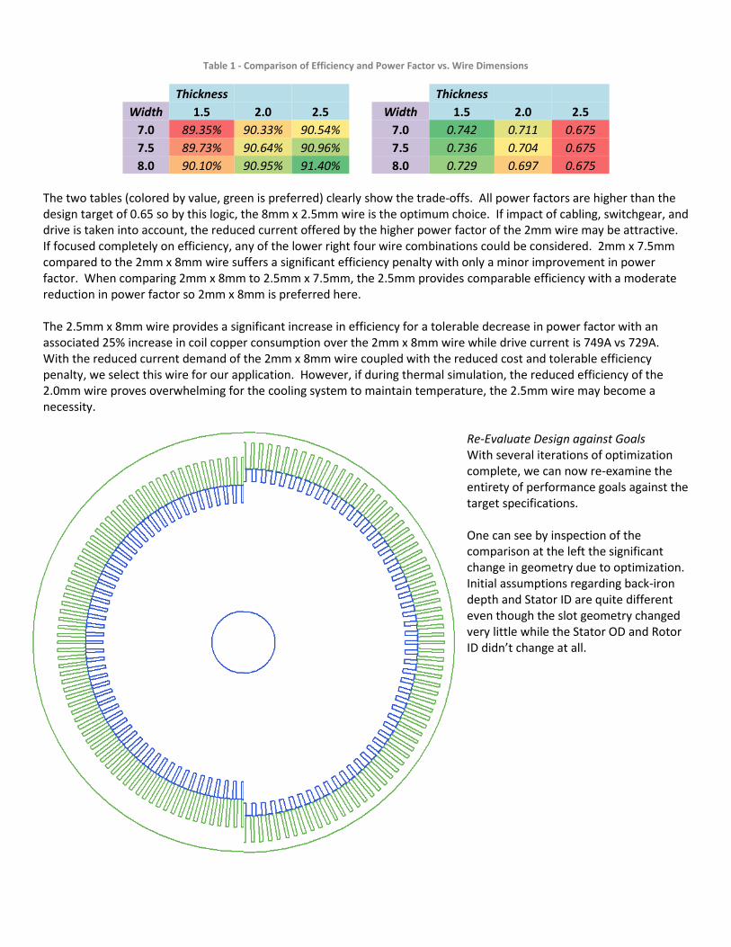
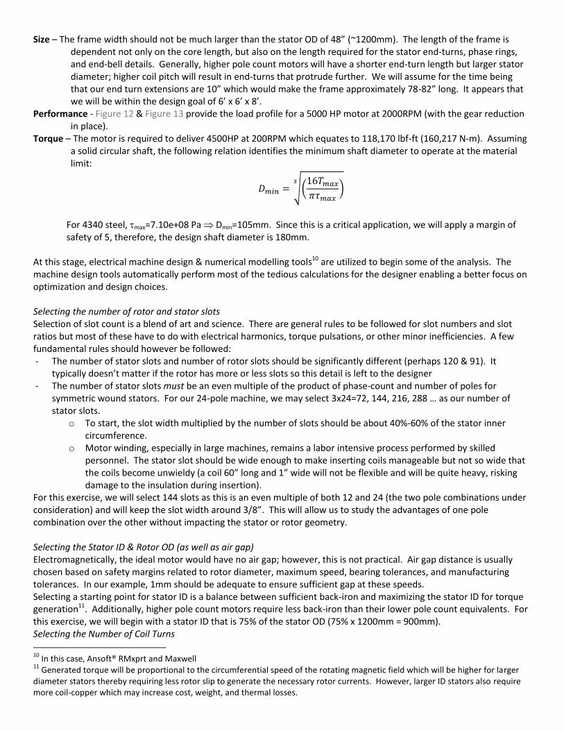
Table 1 - Comparison of Efficiency and Power Factor vs. Wire Dimensions

Thickness

Thickness

Width 1.5 2.0 2.5

Width 1.5 2.0 2.5

7.0 89.35% 90.33% 90.54%

7.0 0.742 0.711 0.675

7.5 89.73% 90.64% 90.96%

7.5 0.736 0.704 0.675

8.0 90.10% 90.95% 91.40%

8.0 0.729 0.697 0.675 The two tables (colored by value, green is preferred) clearly show the trade-offs. All power factors are higher than the design target of 0.65 so by this logic, the 8mm x 2.5mm wire is the optimum choice. If impact of cabling, switchgear, and drive is taken into account, the reduced current offered by the higher power factor of the 2mm wire may be attractive. If focused completely on efficiency, any of the lower right four wire combinations could be considered. 2mm x 7.5mm compared to the 2mm x 8mm wire suffers a significant efficiency penalty with only a minor improvement in power factor. When comparing 2mm x 8mm to 2.5mm x 7.5mm, the 2.5mm provides comparable efficiency with a moderate reduction in power factor so 2mm x 8mm is preferred here. The 2.5mm x 8mm wire provides a significant increase in efficiency for a tolerable decrease in power factor with an associated 25% increase in coil copper consumption over the 2mm x 8mm wire while drive current is 749A vs 729A. With the reduced current demand of the 2mm x 8mm wire coupled with the reduced cost and tolerable efficiency penalty, we select this wire for our application. However, if during thermal simulation, the reduced efficiency of the 2.0mm wire proves overwhelming for the cooling system to maintain temperature, the 2.5mm wire may become a necessity.

Re-Evaluate Design against Goals With several iterations of optimization complete, we can now re-examine the entirety of performance goals against the target specifications. One can see by inspection of the comparison at the left the significant change in geometry due to optimization. Initial assumptions regarding back-iron depth and Stator ID are quite different even though the slot geometry changed very little while the Stator OD and Rotor ID didn’t change at all.

Performance criteria at the base operating point:

Criteria 24-Pole Design Target/Limit Base Power 3.36 MW (4500 HP) - Base Speed 193.9 RPM 200 RPM Base Torque 165,309 N-m (121,930 lbf-ft) 118,170 lbf-ft Base Frequency 40 Hz - Base Voltage 4160 Vrms - Base Current 734 Arms < 715A Net Core Weight 8,284 kg (18,263 lb) < 20,000 lbs Efficiency 90.88% > 93% Rejected Heat 337 kW 253 kW Power Factor 0.692 > 0.7

The table above summarizes the current status of the design; since Base Power, Base Frequency, and Base Voltage were inputs into the simulation, comparisons are omitted. The Base Speed is only slightly less than the design shaft speed of 200RPM (due to slip) – this is easily adjusted by the VFD by increasing output frequency to approximately 41.3 Hz. While improvements in efficiency and power factor were significant, the current requirement is over the target of 715 Arms and the thermal losses are 92 kW (33%) more than originally budgeted. Further optimizations may result in better performance criteria or other adjustments can be made to improve efficiency while degrading power factor (as shown previously). It may also be attractive to re-examine some of the early assumptions (i.e. number of slots, stator OD, etc) in an effort to explore improved design topologies. The following table summarizes the results from a 12-Pole design optimization so that both 12-Pole and 24-Pole designs could be compared.

Table 2 - Comparison of 12-Pole and 24-Pole Designs

Criteria 12-Pole Design 24-Pole Design Target/Limit Base Power 3.36 MW (4500 HP) 3.36 MW (4500 HP) - Base Speed 194.5 RPM 193.9 RPM 200 RPM Base Torque 164,811 N-m (121,560 lbf-ft) 165,309 N-m (121,930 lbf-ft) 118,170 lbf-ft Base Frequency 20 Hz 40 Hz - Base Voltage 4160 Vrms 4160 Vrms - Base Current 632 Arms 734 Arms < 715A Net Core Weight 8,308 kg (18,316 lb) 8,284 kg (18,263 lb) < 20,000 lbs Efficiency 90.90% 90.88% > 93% Rejected Heat 336 kW 337 kW 253 kW Power Factor 0.804 0.692 > 0.7

Table 2 briefly outlines and highlights the performance differences between the 12-Pole design and 24-Pole design motors. Both motors are designed to operate with the same input voltage and provide the same output torque at approximately the same speeds; weight and efficiency are nearly identical between the two machines. One major advantage one might quickly notice is the difference in full load current between the two machines. Higher pole machines of a given size class often suffer from inferior power factors – in some fixed frequency applications, the advantage of a lower shaft speed is worth the extra current capacity needed. For this example, the 12-Pole design enables the use of 14% smaller upstream drives, switchgear, transformers, and cabling than does the 24-Pole design with the only significant difference being the Base Frequency of 20Hz instead of 40Hz. It would be critical to the application to ensure that the drive control algorithms will remain sufficiently stable across 0-20Hz and that the bridge will have sufficient frequency resolution to control shaft speed, but the 12-Pole design would be the most probable selection.

Next Steps Further optimization of the high-level (bulk) parameter design may allow for further improvements in size, weight, or

efficiency. Advanced numerical techniques could also be employed at this time in an effort to find a unique solution to

the parameterized design that improves on one or more of the design criteria – genetic algorithms (GA’s), Non-Linear

Programming (NLP), and Pattern Searches may each result in superior parameter combinations that may have been

missed or over-looked during simple one or two variable sweeps. Once a collection of similar designs have been

compiled, scripting can be employed to automatically generate operating envelope speed-torque-power curves and

efficiency maps that can be used to gain better insight into fitness for the application and potentially identify any design

weaknesses18. Also at this stage of development, a formal design and specifications review should be conducted to

ensure that integrated systems interfaces and inter-dependencies are properly addressed and identified.

Table 3 - 12-Pole, 4500 HP, 4 kV Induction Motor; Efficiency Map

Mo

tor

Po

we

r (a

s %

of

De

sign

)

100% 78.8 87.7 90.2 91.6 92.0 92.1 91.9 91.8 91.4 90.9

90% 77.4 86.8 89.5 90.9 91.6 91.8 91.4 91.2 90.5 90.0

80% 77.0 85.7 89.2 90.3 90.8 90.9 90.7 90.2 89.6 89.0

70% 75.1 84.4 88.1 89.3 89.9 90.1 89.6 89.3 88.6 87.6

60% 72.7 82.7 86.9 88.5 89.1 88.8 88.4 88.0 86.9 85.7

50% 69.6 81.3 86.0 86.9 87.5 87.4 86.9 85.9 84.6 82.9

40% 65.4 79.1 83.5 85.4 85.8 85.7 84.4 83.0 80.8 78.2

30% 59.8 76.0 81.1 83.4 83.2 82.0 80.0 77.2 73.4 65.6

20% 54.6 71.4 78.2 79.3 77.5 74.0 68.3 69.1 68.8 68.6

10% 47.4 67.2 70.0 62.4 45.4 45.2 45.0 44.8 44.6 44.4

10% 20% 30% 40% 50% 60% 70% 80% 90% 100%

Motor Speed (as % of Design)

The efficiency map of Table 3 shows the efficiency trend at various speeds and power levels. Recall from Figure 12 that

the power required will approximate a cubic function; cursory examination of the efficiency map shows that there is a

significant improvement to be implemented during continued optimization to maximize efficiency in the power and

speed ranges of interest (maximum efficiency is centered around 60% speed and 100% power…a region that is usually

not reachable during normal vessel operation). Drive algorithm tuning may also provide some capability to adjust

performance at various speeds and power levels but should only be relied upon for marginal adjustments.

After bulk design is 90% complete and summary performance is accepted, detailed Finite Element Analysis (FEA) on the

electro-magnetic design and Computational Fluid Dynamics (CFD) for thermal design can begin. There is some benefit in

performing magneto-static analysis but the majority of the effort will focus on transient analysis. It is during this stage

that refinements will be made to the slot geometry and laminations to address flux concentrations, enhanced cooling

strategies, and mechanical issues (strength, vibration, mounting, etc). A cyclic, iterative process of transient FEA, CFD,

solid modelling, and numerical modelling is required to finish optimization; the majority of the designer’s time is usually

spent during this phase of design.

18

For example, we notice that the efficiency is worst at low speed/low power operation. This is of little consequence since it is unlikely that the vessel would be operating in this region for extended periods of time. Maximum weight should be given to total expected energy consumption over the life of the vessel (…it makes little since to be most efficient at 100% power if the vessel will operate at 70% power for the majority of its expected life).

Concluding Remarks

Implementation of integrated system design and analysis by component providers can provide systems integrators (and

eventually end-users) with highly optimized, efficient systems that reduce capital costs and life-cycle costs. Most

systems can be appropriately modeled numerically to incorporate cost functions and weighting factors for a wide variety

of criteria. A highly optimized, component designed for single speed use will often be detrimental to a larger integrated

system when operated away from that ideal operating point since system level assumptions used during design are no

longer valid (and are often not provided by the manufacturer nor requested by the systems designer/integrator).

Integrated system-level component design is an engineering philosophy that when applied effectively, can enhance key

criteria for minimal investment (and in some cases, will cost less).

This paper briefly outlines the high level design and selection process for a 5000 HP induction motor for a fictitious

marine propulsion application. By examining the propulsion system as an integrated system, we have shown how an

astute designer can make significant system level design trade-offs that have meaningful impact on capital expense,

maintenance requirements, supporting infrastructure, operation flexibility, design flexibility, and construction flexibility.

While the focus of this paper was on a marine propulsion example, this philosophy can be expanded and extrapolated to

any system where variable speed motor operation is required or might be desired.

The majority of motor designs are generic or ‘general purpose’; the trend over the past decade has been to apply a

variable frequency drive to a general purpose induction motor. Too often, the selected motor has not been optimized

for use in the chosen integrated system nor has it been optimized for use with a variable frequency drive. This article

has presented a straight-forward method using first principles techniques that shows how small, seemingly innocuous

changes in materials or geometry can have significant impact on any of several important operating parameters that

might only occur at a single speed or power level that is not normally considered or that is not listed on a summary label

plate.

Through application of integrated systems analysis, numerical modelling, and collaborative effort among component

providers and systems designers; lighter, smaller, lower cost, more efficient, and higher performing systems can be

created. A critical element to this approach is to enforce an integrated systems methodology at component design

stages by engaging component providers as early as possible in system (or vessel) design and embracing critical analysis

techniques relating to system interaction and inter-operability throughout the design process.

References

A. NEMA MG-1 B. IEEE 112-2004 C. Alger Motor Book D. Handbook of Electric Motors E. The Induction Machine Handbook

integrated systems approach to induction motor selection

Documents