integration of hardware and optimization control for
TRANSCRIPT
Integration of Hardware and Optimization Control for Robotic and Prosthetic Systems
A Dissertation
in partial fulfillment of the requirements
for the degree
Doctor of Philosophy
Submitted to
Rutgers, The State University of New Jersey and
The University of Medicine and Dentistry of New Jersey
Graduate Program in Biomedical Engineering by
Jeffrey Edward Erickson
Under the direction of
Evangelia Micheli-Tzanakou, Ph.D.
And with approval of
___________________
___________________
___________________
___________________
New Brunswick, New Jersey May, 2009

© 2009
Jeffrey Edward Erickson
ALL RIGHTS RESERVED

ii
ABSTRACT OF THE DISSERTATION
Integration of Hardware and Optimization Control in Robotic and Prosthetic Systems
by JEFFREY EDWARD ERICKSON
Dissertation Director:
Evangelia Micheli-Tzanakou, PhD
With medical advances through the past half century, survival rates
following trauma have risen. Along with this rise has come an increase in the
number of survivors with amputated limbs. Many of these survivors are Soldiers,
Airmen, and Marines, who are relatively young and could benefit from
sophisticated prostheses to replace the lost function.
These prostheses would be very maneuverable and able to better mimic
the natural human motions. Such devices would likely be high degree of freedom
with many actuators. Control of prostheses with intelligent algorithms may
provide improved performance for the user.
To this end, a novel experimental transmission for driving the several
joints of such a device has been developed and tested. Also, it has been used in
the design, production, and testing of a 3 DOF digit actuator for use in a
prosthetic hand.
Embedding the control hardware would make such a prosthesis more
compact and portable. Using custom printed circuit boards, Microchip PIC
microcontrollers have been used to control the digit actuator. Taking advantage
of surface mount packages, control boards have been developed which integrate

iii
motor drivers with microcontrollers, and fit into a space comparable to that of
the aforementioned prosthesis. Furthermore, the networking capability of these
controllers has been demonstrated, presenting an extensible framework for
addition of processing power as technology develops.
Given the non-linear nature of the several joints in the system, intelligent
controls have been explored. Model reference adaptive control (MRAC) was used
in simulation of digit models. Also, coupling MRAC with artificial neural
networks yields ANN-MRAC (artificial neural network model reference adaptive
control). Training these ANN control systems using ALOPEX yields good
tracking performance across the non-linear range of the system. Such control
logic may prove effective in a time varying non-linear system such as a hand
prosthesis
Human machine interfacing is key in the use of prostheses. Since a
minimal amount of training is most desirable for the user, adaptive and
intelligent methods may provide a control interface framework that reduces
learning time for the user. To accomplish this, an algorithm for optimization of
large dimensionality sensor grids was developed. This algorithm uses several
template matrices to optimize the gain of each sensor in the grid. This both
identifies a region of activity, and reduces the signal-to-noise ration of the sensor
grid output by reducing gain on channels not containing information. The
desired region is identified through enhancement of the signal gain on the
sensors above the region. This would allow the placement of sensors on the body
in an inexact fashion and instead let the computer optimize the sensor network
gains for regions of activity associated with a given motion. Such an adaptive

iv
system reduces learning time for the user, thus reducing human error and easing
use.

v
Acknowledgement
As with any work, there are a number of people who made this possible.
First, I must thank my two advisors, Mourad Bouzit, Ph.D. and Evangelia
Micheli-Tzanakou, Ph.D. for guiding and supporting this work.
John Petrowski, with the Rutgers University Mechanical Engineering
Department, was instrumental in fabrication of parts, both in the machine shop
and the rapid prototyping facility.
Earlier in my graduate education, I was supported by the United States
Department of Education via a Graduate Assistance in Areas of National Need
fellowship.
FIRST Robotics Competition Team 41, to whom I taught controls and
programming. “You don’t truly comprehend a subject until you teach it.”
ANADIGICS, the company that has employed me for the past two years.
In particular, William Tompkins, Ha Tran, Ruddy Ostin, Ken Casterline, and
others who made available their expertise, advice, and equipment to help me
complete this work.
Kevin P. Granata, a professor of mine at the University of Virginia who was
slain in the Virginia Tech Massacre in 2007. He was the first professor of mine to
bring research into the classroom and gave me the foundation for model
development used in this dissertation.
Of course to my parents and family, who have supported me in many ways
to complete this project.

vi
Perhaps most importantly, the past and present members of the United
States Military and State National Guards I know who inspired me to undertake
the project:
Alan D. Marrero, United States Marine Corps
Michael E. Eagan, United States Army
James Giacchi, New Jersey National Guard
Carl J. Heim, United States Marine Corps
Duane Mantle, United States Army
Hunter Birckhead, United States Army
Joseph Bartnicki, Pennsylvania National Guard
Edward E. Erickson, United States Army
William A. Erickson, United States Army
Thomas E. Donato, United States Army
Wilhelm A. Erickson, United States Army
Salvatore Sacco, United States Army Air Corps

vii
Table of Contents
ABSTRACT OF THE DISSERTATION..................................................ii
Acknowledgement .............................................................................v
Table of Contents.............................................................................vii
List of Figures.................................................................................... x
List of Tables ..................................................................................xiii
Glossary of Terms .......................................................................... xiv
Overview and Objectives ................................................................... 1
1.1 Introduction ............................................................................ 1
1.2 Motivation ............................................................................... 1 1.2.1 General Motivation................................................................................ 1 1.2.2 Implications of Modern Warfare...........................................................2
1.3 Literature Review ....................................................................4 1.3.1 Existing Prostheses................................................................................4 1.3.2 Dynamic System Control ..................................................................... 12 1.3.3 Adaptive Systems................................................................................. 25 1.3.4 Sensors .................................................................................................34 1.3.5 Detecting Volition................................................................................ 37
1.4 Objectives, Goals, and Problem Statement............................. 41 1.4.1 Problem Statement .............................................................................. 41 1.4.2 Objectives.............................................................................................42 1.4.3 Goals ....................................................................................................42 1.4.4 Chapter Summary................................................................................43
Chapter 2: Materials and Methods ...............................................44
2.1 Design Approach ...................................................................44 2.1.1 Mechanical Design...............................................................................44 2.1.2 Actuation..............................................................................................46 2.1.3 Control System..................................................................................... 47 2.1.4 Fabrication...........................................................................................49 2.1.5 Uniqueness ..........................................................................................50
2.2 Design Results .......................................................................50 2.2.1 Mechanical Design...............................................................................50 2.2.2 Motors.................................................................................................. 53 2.2.3 Sensor Tests and Physical Model ........................................................ 55 2.2.4 Embedded Platform Single Joint Control ........................................... 56 2.2.5 Device Hardware Architecture ............................................................ 61

viii
2.2.6 Software Architecture..........................................................................63
2.3 Mechanical Assembly............................................................. 70 2.3.1 Novel Method for Right Angle Transmission ......................................71 2.3.2 Transmission Results .......................................................................... 74 2.3.3 Mounting of Position Sensors ............................................................. 75
2.4 Electronic Hardware Platform............................................... 75 2.4.1 Local Processing .................................................................................. 76 2.4.2 Electrical Characteristics and Board Design....................................... 77
Chapter 3: Control Modeling ........................................................ 81
3.1 Single Joint Control Model .................................................... 81 3.1.1 Derivation of the Equations of Motion................................................82 3.1.2 Extraction of the DC Motor Model......................................................83 3.1.3 Model Implementation and Verification.............................................86 3.1.4 Commentary on the Non-Linearity .....................................................88
3.2 Linear Control of the Non-Linear Single Joint System ...........89
Chapter 4: Model Reference Adaptive Control .............................. 91
4.1 With Linear Model Reference Error Feedback .......................93
4.2 With Squared Model Reference Error Feedback ....................94
4.3 ANN-MRAC: Artificial Neural Network – MRAC .................... 95 4.3.1 Matrix Implementation of Neural Networks in MATLAB..................96 4.3.2 ANN-MRAC Using a 2-3-2 Feed Forward ANN .................................98 4.3.3 Use of a 2-4-2 Feed Forward Artificial Neural Network................... 103
4.4 Variation of the Training Parameters .................................. 105
Chapter 5: ALOPEX Optimization of Sensor Networks ............... 108
5.1 Rationale of Optimization.................................................... 108
5.2 Optimization Algorithm....................................................... 109
5.3 Response Function ............................................................... 111
5.4 Optimization.........................................................................114
5.5 Computational Efficiency and Application ............................ 121
Chapter 6: Conclusions and Future Work................................... 122
6.1 Conclusion............................................................................125
6.2 Future Work........................................................................ 126 6.2.1 Extension to Multi-Joint Control ...................................................... 126 6.2.2 Construction and Testing of a Complete Artificial Hand...................127 6.2.3 Extension of the Electronic Hardware ...............................................127
References ..................................................................................... 129

ix
Curriculum Vita .............................................................................137

x
List of Figures
Figure 1.1: Southampton Capstan Drive .................................................................. 5
Figure 1.2: Schematic of the FZK Hydraulic Balloon Mechanism ..........................6
Figure 1.3: MANUS Crossed Tendon Mechanism Schematic ................................ 7
Figure 1.4: The Dextra Prosthesis System ...............................................................8
Figure 1.5: The Shadow Dexterous Hand ................................................................9
Figure 1.6: Cyberhand ............................................................................................ 10
Figure 1.7: The University of Victoria Biomimetic Finger Actuator ......................11
Figure 1.8: Root Locus of Example Transfer Function ......................................... 16
Figure 1.9: Bode Plot of Example Transfer Function .............................................17
Figure 1.10: Illustration of the Conformal Mapping z=exp(sT) ............................ 19
Figure 1.11: Detail of the Southampton Integrated Force Slip Sensor ..................36
Figure 1.12: Example of EMG Time Course for Control of the MANUS Device ...38
Figure 1.13: State Machine Diagram for Control of the FZK Hand.......................39
Figure 1.14: MKI Concept Illustration ...................................................................40
Figure 2.1: Proposed Mechanical Configuration of the Digits ..............................44
Figure 2.2: MRF Piston.......................................................................................... 47
Figure 2.3: Initial and 5th Evolution Finger Designs............................................ 51
Figure 2.4: Example of Detail Available Through Solid Modeling ....................... 52
Figure 2.5: Sanyo 12GN-0348 Motor .................................................................... 54
Figure 2.6: Kinetic Model for Testing of Control System...................................... 55
Figure 2.7: Hall Effect Sensor Linearity ................................................................ 56
Figure 2.8: The Effect of Filtering on Data............................................................58
Figure 2.9: Constant Velocity Control Data Plots ................................................. 59

xi
Figure 2.10: Proportional Feedback Control Data Plots .......................................60
Figure 2.11: Block Diagram of Hardware and Software Architecture...................62
Figure 2.12: Overview of Controller Test Platform................................................62
Figure 2.13: Block Diagram of Coordinating Processor Software.........................66
Figure 2.14: Block Diagram of Embedded Controller Software............................ 67
Figure 2.15: USB Packet Structure.........................................................................69
Figure 2.16: Block Diagram of High Level Processor Software.............................70
Figure 2.17: Right Angle Transmission Test Platform and Miniaturized Form ... 72
Figure 2.18: Joint in Assembly Jig......................................................................... 73
Figure 2.19: Completed Finger in Testing Mount ................................................. 75
Figure 2.20: Embedded Processor Printed Circuit Boards ................................... 78
Figure 3.1: Schematic of Forces and Intertia Acting on Single Joint ....................86
Figure 3.2: Simulink Model of the DC Motor ........................................................87
Figure 3.3: Output of DC Motor Modeling After Adjustment of the Back EMF
Constant .................................................................................................................87
Figure 3.4: Graph of Linearity Measure of Sine Function ....................................88
Figure 3.5: Model Trajectory Under Linear PI Control.........................................90
Figure 4.1: Simulink Model for MRAC ..................................................................92
Figure 4.2: MRAC Output Using Linear MR Error Adjustment ...........................93
Figure 4.3: MRAC Output Using Squared MR Error for Adjustment...................94
Figure 4.4: Simulink Model for ANN-MRAC ........................................................95
Figure 4.5: 2-3-2 ANN-MRAC Results Using Last 500 Error Points as Response
................................................................................................................................99

xii
Figure 4.6: 2-3-2 ANN-MRAC Result Using Last 500 and First 500 Error Points
as Response .......................................................................................................... 100
Figure 4.7: 2-3-2 ANN-MRAC Response Using Gain Scheduling........................101
Figure 4.8: 2-3-2 ANN-MRAC Results Using Full RMS Error ........................... 102
Figure 4.9: 2-4-2 ANN-MRAC Result During Training ...................................... 103
Figure 4.10: 2-4-2 ANN-MRAC Result After Full Training Time ....................... 105
Figure 4.11: Results for the High Learning Rate Parameter Case....................... 106
Figure 4.12:Results for the High Training Noise Case ........................................ 107
Figure 5.1: Plot of Field Intensity vs Distance ......................................................110
Figure 5.2: Results of Sensor Optimization for the Center Case..........................115
Figure 5.3: Response vs. Iteration plot for the Center Case.................................116
Figure 5,4: Field Optimization Result for the Edge Case .....................................118
Figure 5.5: Response vs Iteration plot for the Edge Case.....................................119
Figure 5.6: Field Optimization and Response vs. Iteration Plot for the Corner
Case........................................................................................................................121

xiii
List of Tables
Table 1.1: United States Battlefield Casualties 1941-2008…………………………………3
Table 3.1: Motor Electrical Characteristics………………………………………………….. 83
xiv
Glossary of Terms
ADC – Analog to Digital Converter. Electronic hardware, found often in embedded processors, that converts analog signal values to digital numbers for use in the processor.
ALOPEX – Algorithm for Pattern Extraction or Algorithmic Logic of Pattern Extracting Crosscorrelations. A correlation based optimization algorithm that uses previous changes in local weights correlated with changes in global response to determine future values.
ANN – Artificial Neural Network. A biologically inspired computational method using multiple interconnected nodes exhibiting high parallelism, like that of the brain.
Computational Intelligence – A subset of adaptive algorithms that exhibit adaptation based on biological intelligence.
Embedded System – A special purpose processor or network of processors that perform a specific task with high computational efficiency. Ethernet devices, GPS receivers, and portable digital music players are examples of embedded systems.
FDM – Fused Deposition Modeling. A three dimensional printing technique that uses a melted filament of plastic to generate parts from computer solid modeling data.
Hall Effect Sensor – A sensor that detects magnetic field. Coupled with specialized magnets, Hall Effect sensors can be used to detect position.
I2C – Inter Integrated Circuit Bus. A two wire bus for serial communication between processors and peripheral devices.
MRAC – Model Reference Adaptive Control. An adaptive control approach that uses a computed reference model response as a target for system tracking.
PCB – Printed Circuit Board. A planar board with selected regions of copper plating used to connect integrated circuits without the need to wire each individual pin.
PIC – Peripherical Interface Controller. A series of embedded processors used for acquisition and control. Being application specific, they do not have an operating system and are typically programmed in either C or assembly.
PWM – Pulse Width Modulation. A method for communicating output voltages, particularly to a motor, using a pulse at regular intervals. The length of the pulse corresponds to voltage.
Prosthesis – A specialized device, sometimes robotic, for the replacement or enhancement of human function.

xv
Surface Mount Technology – An integrated circuit packaging technology that mounts devices to the surface of a circuit board rather than through holes in the board.
Through Hole Technology – An integrated circuit packaging technology that mounts devices via regularly spaced holes in a circuit board. Generally regarded as legacy.
USB – Universal Serial Bus. An industry standard serial communication bus for communication between general purpose processors and peripheral devices
WCIR – Wounded to Combat Injured Ratio. The ratio of wounded in action to the sum of wounded in action to killed in action. An indication of survivability following a battlefield injury.

1
Overview and Objectives
1.1 Introduction
Those of us who have full use of our hands may take for granted the value of our
dexterity. We do not think twice about how to open a door, open a bottle, shake a
hand, or pick up a cup of coffee. For those who have lost a hand, these can be
very frustrating tasks, especially for those who lost the hand suddenly and
traumatically.
Technology has progressed to the point where devices that have the dexterity of
the hand, measured in degrees of freedom (DOF), can be artificially produced.
Also, electronics have progressed to the point where major processing power can
be packed into increasingly smaller spaces. These combine to provide the
platform for the development of an artificial prosthesis capable of mimicking the
natural human hand (Pons, et al, 1999 & Craelius, 2002).
1.2 Motivation
1.2.1 General Motivation
Amputations have been a medical practice since the middle ages (Mitchell,
2004). Over time, the understanding of the human forearm has allowed for neat
surgical procedures that effectively form the residuum to a shape that can be
accepted by a prosthesis. That device, however, had been rather archaic until
recently, usually resembling a hook or a purely cosmetic hand. The end actuators
typically needed to be specially designed for individual tasks. As a result, the

2
prosthetics that amputees received either were pleasing to the eye or functional,
but rarely both.
The late 20th century brought advancements in prosthetic technology. Gone were
the hooks and clamps of earlier times, replaced with hands that were both
cosmetic and functional. These hands, while offering more dexterity than
previous devices, still did not approach the dexterity of the natural hand. This
project seeks to develop a prosthesis that approaches the performance, force
generation, and dexterity of the natural human hand.
1.2.2 Implications of Modern Warfare
Though many groups of people are subject to amputation, there are a few groups
that are especially prone to needing the procedure. Power line workers can
literally have their hands vaporized by electricity, factory workers can have their
hands traumatically amputated by machinery, and soldiers can lose entire limbs
to battlefield injury.
Ironically, the development of more effective weapons has been accompanied by
better medical technology (Hartcup, 2000) and logistics (Lynch et al, 2005) in
the military. In World War II, battlefield medicine took on a new sophistication
with the large scale training of medics for immediate medical care (Andersen,
2003). However, depending on the theater, a wounded soldier could find himself
laying on a cot near the front for many days before being transported by air,
truck, or ship to rear hospitals (Cowdrey, 1994). During the Vietnam and Korean

3
Wars, the use of the UH-1 “Huey”, HH-3 “Jolly Green”, CH-53, and HH-53
helicopters brought fast evacuation from the front line (Wetterhahn, 2001), but
still left most casualties in country for many days and perhaps weeks.
The conflicts of the past decade have brought a heretofore unseen speed to
military medical treatment. Helicopters, namely the HH-60 Pave Hawk,
continue to be used in Iraq for evacuation (Boyne, 2003). Rather than even
staying on the continent the soldier was wounded on, many of those wounded
find themselves in the continental United States within a week. Casualties are
almost immediately evacuated from the fighting, are on a medical ship by the end
of the day, and are in Germany or the United States by the end of the week,
sometimes sooner. Typically this is done by fixed wing jet (Boyne, 2003). As a
result, the ratio of casualties to deaths has risen; more people injured in combat
are surviving (see Table 1.1). This has generated added demand for effective
dexterous prosthetics so our surviving Purple Heart recipients may lead
productive lives after their discharge.
Table 1.1: United States Battlefield Casualties 1941-2008.
WWII Korea Vietnam War on Terror
Iraq
KIA 292,131 33,629 47,072 358 3609
WIA 671,801 103,284 155,419 (303,704)
2330 30,324
WCIR* 69.7% 75.4% 76.7% (86.6%)
86.7% 89.4%
For Vietnam data, numbers in parentheses refer to total WIA, numbers without parentheses refer to hospitalized WIA. “War on Terror” refers to conflicts in the Global War on Terror,
including Afghanistan, but excluding Iraq. *WCIR: Wounded to Combat Injured Ratio (WIA/(WIA+KIA)).
WWII (p. 956), Korea (p.1216), and Vietnam (p.1322) data from Codfelter, 1992. War on Terror and Iraq War data from Wikipedia (2008) and United States Department of Defense
(2008).

4
1.3 Literature Review
1.3.1 Existing Prostheses
Prosthetic devices have existed for centuries, brought to popular attention by
Captain Hook, of Peter Pan fame. Indeed, early prosthetics were simple devices
that were either purely functional, like hooks, or purely cosmetic, like a
mannequin’s hand. Otto-Bock is a well known manufacturer of such hands,
including a simple grasp actuator. However, there are more advanced prostheses
in existence or in development, ranging from the simple and ultra light design of
the VA Rehabilitation and Research and Development Center in Palo Alto, CA
(Doshi et al, 1998) to the extremely dexterous (but heavy) design of the Shadow
Robot Company in England.
1.3.1.1 The Southampton Hand
Calling any one particular device “The Southampton Hand” is actually a
misnomer. There have been several hands developed at the University of
Southampton, England since the first in 1967. The Southampton Team prefers to
describe “The Southampton Hand” as a general philosophy regarding prosthetic
hands, the design targets, and the extraction of volition from patient data. The
core of this principle is the Southampton Adaptive Manipulation Scheme (SAMS)
(Light et al, 2002), the method of data extraction.
In terms of the physical device, the most recent hand appeared in the literature in
2000 (Light and Chappell, 2000). It uses SAMS as the core of the control

5
system. The digits are actuated using DC motors with capstans, for force
amplification (Figure 1.1(a)). There are five independent digits, but the digits are
internally coupled using wires and linkages in each digit, and fold with consistent
trajectory (Figure 1.1(b)). In
addition, the thumb has a
circumduction (a combination
of axial rotation and abduction-
adduction) actuator (Light and
Chappell, 2000).
This system, the Southampton-
Remedi hand, weighs 400g, has
6 DOF, and has a total grip
force of about 40N. Each of the
four digits actuate with a peak
active grip force of 9.2N, while
the thumb has a peak active grip force of 3.7N. At peak utilization, the device
draws 10.5W of electrical power (Light and Chappell, 2000). This design gained
much press, through the BBC, in 2005.
1.3.1.2 The Hydraulic FZK Hand
In 2001, Schulz et al reported on their development of a hydraulically actuated
hand. The system is biomimetic, based on the activity of insects. Small
hydraulic balloons were placed in the vertex of each joint, and inflated to open
(a)
(b)
Figure 0.1: Capstan drive used in the Southampton Hand (a) and linkage detail (b). (Kyberd et al, 2005)

6
the joint (Figure 2-2). This is essentially the same principle arachnids use to
move their appendages.
In 2004, the same group at
Forschungszentrum Karlsruhe (FZK)
in Germany expanded the scope of
their hydraulically driven hand, and
applied it to prosthetics (Pylatiuk, et
al, 2004). One key aspect of the
design is a preshaping step to prepare
the hand for the activity. This
required initial user input.
The physical device weighed 891g, with 15 DOF, and a maximum grip force of
65N. Each digit contributed approximately 8N, provided by 15 independent
flexible fluidic actuators, the hydraulic balloons described above (Schulz et al,
2005). Data on the compressor, the fluid used, and the power consumption were
not provided.
1.3.1.3 The MANUS Hand
Although also used to describe a hand developed at MIT, this MANUS hand is
attributed to a European and Asian consortium in Spain, Belgium, and Israel.
Like the aforementioned hands, it uses EMG data to control the system. This
hand, along with Dextra and the Southampton Hand, was developed in the late
Figure 0-2: Conceptual schematic of the inflatable hydraulic balloon mechanism (Schulz et al, 2001).

7
1990’s, and reflects the technology of the time. Only the first two digits and the
thumb are independently actuated. The digits use a crossed pulley system to
approximate a tendon. The thumb uses a Geneva Wheel mechanism to allow for
4 degrees of freedom. In addition, rotation about the wrist is possible through
the use of thin ultrasonic motors (Pons et al, 2005(a)). This gives the MANUS
device a total of 6 DOF in the hand (driven by 10 brushless DC motors), and 1
DOF (pronation-supination) in the wrist (through high torque ultrasonic
motors), for a total of 7 DOF (Pons et al 2005(a)).
1.3.1.4 The Dextra Hand
Dextra was developed by Dr. William Craelius at Rutgers University in the late
1990’s. The hand itself is actuated using commercially available servo motors.
All five digits are independent of one another, but curl with consistent trajectory.
The novelty of the Dextra system lies in the detection method. Rather than using
EMG signals, pressure information from the residuum is used to detect volition.
Figure 0.3: "Crossed Tendon Mechanism" schematic (Pons et al, 2005).

8
This overcomes the noise susceptibility of EMG, bypasses the cost of implanted
sensors, and demodulates the inherently frequency modulated information from
the nervous system. Formally, the method is referred to as “Residual Kinetic
Imaging” or a “Myo-Kinetic Interface” (Curcie, et al, 2001 & Phillips and Craelius,
2005). These signals are then used to construct drive signals for the prosthesis
itself, which is driven by servomotors, as mentioned. Application of this system
to actual amputees has proven successful, insofar as an amputee can play simple
tunes on a piano with minimal practice.
Figure 0.4: The Dextra Prosthesis System (Craelius, 2002). The top piece is the sleeve for the residuum; at middle right is the rigid socket; at middle left is the microcontroller; the
bottom is the hand with servo actuators.

9
1.3.1.5 The Shadow Dexterous Hand
The Shadow Hand is a commercially produced hand from England. The
developers used pneumatic artificial muscles to give each digit 4 DOF. The
thumb is enhanced with another joint
and muscle, giving it 5 DOF. Further,
the wrist is actuated with two motors
(Shadow, 2005). These many degrees
of freedom very closely approximate
the DOF of the natural human hand,
making Shadow the robotic hand
design to beat. Unfortunately, the
system weighs 3.5kg, and the
compressor, controls, and actuator
take up too much space in the palm
and forearm to allow a socket for the
residuum.
The system has, however, found research applications in academia, and
applications for climbing and walking robots (Shadow, 2003). Speaking strictly
in terms of functionality, the Shadow hand meets and surpasses the criteria for a
prosthetic. Further, the controller for the hand is compliant with standard IEEE
protocols, namely IEEE 1394 “Firewire” (Shadow, 2004). This standardization
Figure 0.5: The Shadow Dexterous Hand (Shadow, 2005).

10
makes the product marketable to a wide audience. However, the high weight
prohibits its use as a viable prosthetic.
1.3.1.6 Cyberhand
A group at the Scuola Superiore Sant’Anna in Pisa,Italy has also developed a high
degree of freedom manipulator for use as a prosthesis, which they dub the
“Cyberhand.” The approach of this design is to maximize the degrees of freedom
available in each digit by using a
separate actuator for each joint. Using
linear precision microdrivers based on
brushless DC motors with planetary
transmissions and lead screw drive
(Smoovy), the actuators can be placed
within the digit’s links. The system
also employs several sensors,
including Hall Effect sensors for
position, and force sensors on the
digits (Carrozza et al, 2002). In a
separate report (Carrozza, et al, 2006), Cyberhand’s actuation is described as one
similar to the Southampton hand (above), driven by pulleys along with actuators
by Minimotor, similar to the Smoovy unit with an added incremental encoder. It
is important to note that the Cyberhand digits are “underactuated” (Cipriani,
2006). This is to say that the number of actuators is less than the number of
Figure 1.6: Cyberhand grasping a plastic cup.
11
degrees of freedom, to simplify control for the human wearer of the device
(Micera, et al, 2006).
In terms of the control method, the Cyberhand group uses pulse width
modulation (PWM) to drive the DC motors they use. These signals are generated
by Microchip PIC18F2431 processors, and employ supervisory control via
computer (Cipriani, et al, 2008). Communication between the PIC and the
supervisory computer is handled by RS-232 serial protocol (Cipriani, et al, 2006).
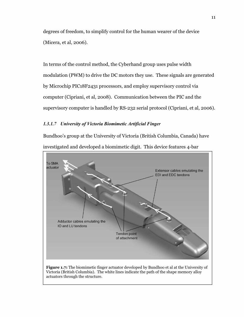
1.3.1.7 University of Victoria Biomimetic Artificial Finger
Bundhoo’s group at the University of Victoria (British Columbia, Canada) have
investigated and developed a biomimetic digit. This device features 4-bar
Figure 1.7: The biomimetic finger actuator developed by Bundhoo et al at the University of Victoria (British Columbia). The white lines indicate the path of the shape memory alloy actuators through the structure.

12
linkages for the joint construction, and shape memory alloy actuators. In
addition, they used what they term “PWM-PD” control, or pulse-width-
modulated proportional derivative control.
Using the linkage at each joint allows the finger joints to articulate properly, and
the shape memory alloy mimics tendons. The shape memory alloy material is
compliant, and springs are used to provide tension. Using PWM shows a direct
route for the control of the digit, as many processors, including those available
from Microchip (2008), have pulse width modulated output features. The
structure of the digit was constructed using solid modeling and rapid
prototyping, namely stereolithography (SLA).
1.3.2 Dynamic System Control
Broadly looking at control systems simplifies the discussion of the theories
behind them. Rather than classifying the actuators into their output categories
(force, motion, etc.), separating them based on internal characteristics (linear vs.
non-linear) allows for a more orderly coverage of the topic. Below, traditional
and modern control of linear systems is covered, as well as the use of adaptive
mechanisms, including neural networks and model reference adaptive control.
1.3.2.1 “Traditional” Control of Linear Time Invariant (LTI) Systems
Unfortunately, very few real world systems are linear. Many of these non-
linearities can be modeled through approximations as linear systems. If a system
can be modeled as a linear combination of inputs and outputs, and the

13
derivatives of the inputs and outputs, of the system, it is considered linear time
invariant (LTI). This linear model must take the form:
(1.3.1)
That is, the general form of an LTI system is a differential equation that is a sum
of the inputs and outputs and their derivatives. The solution of this differential
equation is best found using the Laplace transform. Particularly with regard to
derivatives, the Laplace Transform has the following property:
(1.3.2)
So, the Laplace Transform makes a differential equation in the time domain a
polynomial equation in the s-domain.
Transforming the model 1.3.1 from the time domain to the s-domain yields the
following result:
(1.3.3)
This is the general form of a polynomial of order M on the left side, and a
polynomial of order N on the right side. M is the “order” of the system, and the
difference (M-N) is the “degree” of the system. Factoring these polynomials
restates 1.3.3 as products rather than sums:
(1.3.4)
)0()()( yssYtydt
d LT −→
∑∑==
=N
n
n
n
M
m
m
m sXsbsYsa00
)()(
∏∏==
−=−N
j
j
M
i
i zssXpssY00
)()()()(
∑ ∑= =
=M
m
N
nn
n
nm
m
m txdt
dbty
dt
da
0 0
)()(

14
Mainpulating 1.3.4 to isolate the product terms is considered the canonical form
for this equation:
(1.3.5)
Where the pi are the poles of the system, and the zj are the zeros of the system. In
this form, the quotient in 1.3.5 is the Transfer Function of the system. By
definition, the transform function is the Laplace transform of the impulse
response of the system.
The location of the poles and zeros of the transfer function are important in the
analysis of the system. If all the poles are in the left-half plane of the s-plane
(Res<0), then the system is considered “stable,” meaning that for a bounded
input, the system will have a bounded output. If all the zeros of the system are in
the left half plane (Res<0), then the system is invertible. Further, if all of the
poles and all of the zeros of the system are stable (i.e. in the left half plane), then
the system is said to be “minimum phase” (Porat, 1997, pp.262-263).
Fortunately, the control of linear time invariant systems is analytical, well
studied, and well established. Further, there are many methods for controlling
linear systems: Root Locus, Lead/Lag, PID, and State Space (Franklin et al,
2002).
∏
∏
=
=
−
−
=M
i
i
N
j
j
ps
zs
sX
sY
0
0
)(
)(
)(
)(

15
For the following examples, consider the second order system model:
(1.3.6)
And, following the procedure above, the corresponding transfer function is:
(1.3.7)
Which, according to the above equations has zeros at s=-5 and poles at s=-
0.5±j3.1225.
The root locus is a plot of pole and zero trajectories on the s-plane (Laplace
Transform space) as a proportional feedback gain, K, varies. By specifying the
desired damping ratio and natural frequency or time constant and damped
frequency, one can choose the regions on the s-plane that satisfy the
specification, and choose K so the pole trajectory is in the desired section of the s-
plane.
)(5)()(10)()(2
2
txtxdt
dtyty
dt
dty
dt
d+=++
10
5)(
2 +++
=ss
ssG

16
The Lead/Lag controller uses bode analysis to design filters to alter the phase
margin and gain margin of the system. Phase margin is approximated as 100
times the damping ratio, and gain margin is an indication of stability. A lagging
system has a low frequency pole and a high frequency zero, and changes the 0dB
crossing in the bode magnitude plot, which in turn alters the phase margin. A
leading system has a low frequency zero and a high frequency pole, and changes
the -180° crossing in the bode phase plot, which in turn alters the gain margin.
These two system types (leading and lagging) can be used individually or in
combination, leading to the general Lead/Lag controller philosophy.
-20 -15 -10 -5 0 5-6
-4
-2
0
2
4
6Root Locus of Sample Transfer Function
Real Axis
Imaginary Axis
Figure 0.8: Root Locus of the above transfer function.

17
Proportional-Integral-Derivative (PID) control is an approximation of Lead/Lag
control where the proportional gain (P) alters the gain characteristics, and the
integral (I) and derivative (D) gains alter the phase characteristics. Intuitively,
PID control can be seen as a three step process: 1. alter P to make the system
stable, 2. alter I to reduce steady state error, 3. alter D to improve the system time
response. The major pitfall in this method is that the value of the integral gain (I)
can make the system unstable, so there is usually a trade off between steady state
error and system time response.
-40
-30
-20
-10
0
10
Magnitude (dB)
10-1
100
101
102
-135
-90
-45
0
45
Phase (deg)
Bode Diagram of Sample Transfer Function
Frequency (rad/sec)
Figure 0.10: Bode Plot of the above transfer function.

18
1.3.2.2 “Modern” Control of Linear Systems
The above methods are considered “traditional” control, in that they use
frequency or Laplace data to design the controller. In both cases, an
approximation is made to move the poles and zeros of a “black box” system to
desired positions on the s-plane, or on the jω-axis. However, an algebraic
solution to deterministically and accurately place the poles would be preferred.
In addition to this desired pole placement, robust modeling of the discrete time
systems and development of associated controllers is also desirable. This
problem arose in the second half of the 20th century, and lead to the development
of the z-Transform, a corollary to the Laplace Transform, but for discrete time
systems. Jury provides the background mathematics, including the stability and
causality criteria in his work (Jury, 1964).
Converting from the continuous time models to the discrete time models can be
done by several methods (Phillips and Nagle, 1998). Among this are the bilinear
transform and pole reassignment. Bilinear transformation approximates the zero
order hold (ZOH) typically encountered in computer outputs. Pole reassignment
uses conformal mapping to translate the s-plane into the z-plane. The function
for this mapping is z = exp(sT), where z is the complex value of the pole on the z-
plane, s is the complex value of the pole on the s-plane, and T is the sampling
time in seconds. Essentially, this takes the stable poles in the s-plane (Res<0),
and assigns them to the stable region in the z-plane (|z|<1), while incorporating
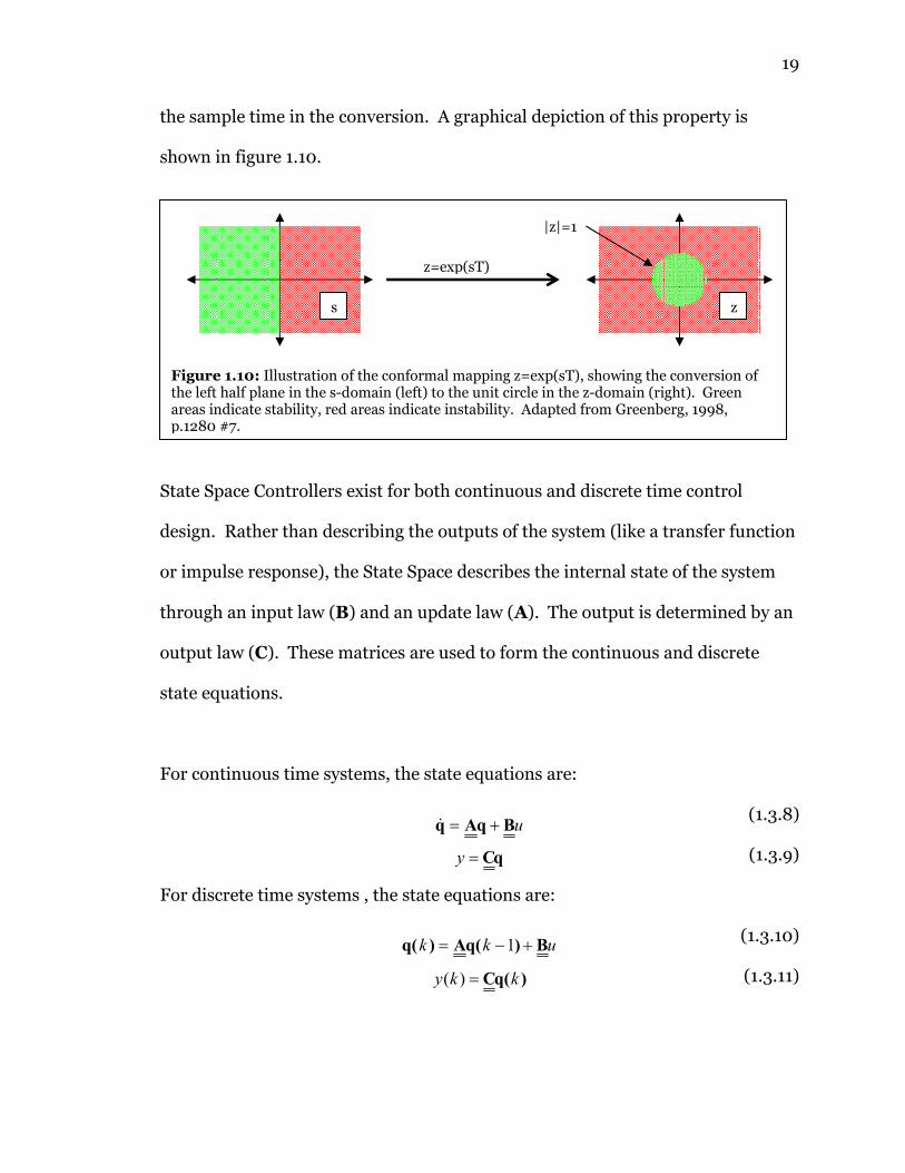
19
the sample time in the conversion. A graphical depiction of this property is
shown in figure 1.10.
State Space Controllers exist for both continuous and discrete time control
design. Rather than describing the outputs of the system (like a transfer function
or impulse response), the State Space describes the internal state of the system
through an input law (B) and an update law (A). The output is determined by an
output law (C). These matrices are used to form the continuous and discrete
state equations.
For continuous time systems, the state equations are:
(1.3.8)
(1.3.9)
For discrete time systems , the state equations are:
(1.3.10)
(1.3.11)
uBqAq +=&
qC=y
ukk B)q(A)q( +−= 1
)q(C kky =)(
Figure 1.10: Illustration of the conformal mapping z=exp(sT), showing the conversion of the left half plane in the s-domain (left) to the unit circle in the z-domain (right). Green areas indicate stability, red areas indicate instability. Adapted from Greenberg, 1998, p.1280 #7.
|z|=1
z=exp(sT)
s z

20
The size of these matrices are determined by the system properties. For a system
of order N with V inputs and W outputs, the matrix properties are:
(1.3.12)
In other words, A is a square NxN matrix, B is a matrix with V columns and N
rows, C is a matrix with N columns and W rows, and q is a column vector with N
elements.
The members of these matrices can be found in at least two ways. First is to
generate the matrix members from the differential or difference equations
directly, specifying the state as a column vector of system variables and their
derivatives (for continuous time) or previous variable values (for discrete time).
Another method is to specify the members from the transfer function. Several
canonical forms for this exist, and methods for translating the s-domain and z-
domain values to the state space are known (Phillips and Nagle, 1998).
Restating equation 1.3.6 from above, and isolating the highest order term yields:
(1.3.13)
The dot notation indicates differentiation in time. From this form of the system
model, we can choose a state vector q and hence its derivative:
(1.3.14)
(1.3.15)
1NWNNVNN q,C,B,A ×××× ℜ∈ℜ∈ℜ∈ℜ∈
)(5)()(10)()( txtxtytyty ++−−= &&&&
=
)(
)()(
ty
tyt
&q
=
)(
)()(
ty
tyt
&
&&&q

21
The update law (A) describes the characteristic equation of the system and is
found through evaluation of 1.3.13, disregarding the input terms.
(1.3.16)
Restating this differential equation through a matrix-vector representation
yields:
(1.3.17)
Where the top row of the matrix in 1.3.17 follows from 1.3.16, and the bottom row
is an identity for the first derivative of y.
Note that the left hand side of 1.3.17 is the derivative of the state, and the column
vector in the right multiply on the right hand side is the state. The equation
1.3.17 can therefore be restated in matrix form as:
(1.3.18)
(1.3.19)
The determinant of A is the system’s characteristic function. So, knowing the A
matrix also specifies the denominator of the transfer function. A relationship
between the state space and the transfer function is given by:
(1.3.20)
For the example system, the center term of 1.3.20 evaluates as:
(1.3.21)
yyy 10−−= &&&
−−=
y
y
y
y &
&
&&
01
101
x
+
−−=
1
4
01
101qq
[ ]q10=y
BA)IC( 1−−= ssG )(
+
−
++=
−
+=−
−
−
11
10
10
1
1
1012
1
s
s
sss
ss 1
A)I(

22
The input and output laws (B and C, respectively) specify the numerator of the
transfer function. The choice of B and C are not necessarily unique, and in the
model system, the following vectors satisfy the requirement for 1.3.20 to evaluate
to the transfer function:
(1.3.22)
(1.3.23)
Note that the result in 1.3.23 corresponds to the transfer function in 1.3.7.
Jürgen Ackermann first published detailed work on discrete control systems in
1972, with an English translation published in 1985 (Ackermann, 1985). His
work provides the mathematical foundation and proof for deterministic pole
placement. The methods he describes include pole placement for both
controllers and observers, given desired characteristic equations for each,
respectively.
The characteristic equation can be altered by applying a control law K. The
control law is a vector which selectively feeds back a sum the states and subtracts
the sum from the input. This so called “full state feedback” alters the
characteristic equation:
(1.3.24)
[ ]10,1
4=
= CB
[ ]10
5
1
4
11
1010
10
122 ++
+=
+
−
++ ss
s
s
s
ss
BBK)AIC( 1−+−= ssG )(

23
Such an alteration is only possible if the system is “controllable.” A system is
controllable if and only if:
(1.3.25)
In other words, the controllability matrix must be invertible in order for the
system to be controlled using the control law K.
The method for finding K is Ackerman’s Method. Given the state matrices A, B,
C, and a desired characteristic equation (transfer function denominator) αc(s),
the control law can be found:
(1.3.26)
This method relies on having access to the internal state of the system. In the
case of a DC motor, for example, the state is the angular position and angular
velocity of the shaft. If the state cannot be directly measured, the state space
representation has the advantage of a construct called the estimator. Estimators
(also called observers) either estimate the current state or predict a future state.
Fundamentally, the observer approximates (estimates) the current state q:
(1.3.27)
(1.3.28)
Where A, B, C are the state space matrices, K is the control law, chosen as given
above, and G is an estimation matrix chosen such that:
(1.3.29)
[ ] 0BABAABB1N2 ≠−
L
[ ][ ] (A)BABAABB100K1N2
cα1−−= LL
qq ~≈
yu GBqGC)BK(A1)(nq −+−−=+ ~~
( ) 0qqt
=−∞→
~lim

24
There are several methods for designing estimators, including Ackerman’s
Method, Least Squares Method, and the Kalman Filter (Phillips and Nagle, 1995).
In Ackermann’s method, the G matrix can be chosen if the system controllability
matrix is invertible:
(1.3.30)
If the controllability matrix is invertible, and given A, B, C, and a desired
characteristic estimation function αe(s), the control law can be found using
Ackermann’s method for observers, which is a corollary to Ackermann’s method
for controllers:
(1.3.31)
Ackerman’s Method is of special importance, because for a controllable
observable system, Ackerman’s method for pole placement allows the design to
use a specified characteristic equation, αc(z). Assuming that the control gains are
realizable by the control processor (or other controlling device), Ackerman’s
method will move the poles of the system to the desired location through an
analytical method.
0
CA
CA
CA
C
≠
−1
2
N
M
=
−
− 1
0
0
CA
CA
CA
C
(A)G
1
1N
2M
M
eα

25
The Kalman Filter is also of special importance, as it creates the optimal
observer. This does not necessarily mean the optimal response, but it is a
method to find the optimal controller in high noise or high interference
environments, taking into account stochastic phenomena. The goal in both these
methods, and for any other estimator, is to approximate the internal state of the
system based on the inputs, outputs, and previous estimation(s).
Control can also be accomplished through adaptive and intelligent systems.
Adaptive systems have the advantage of being able to compensate for unknown
or changing system parameters. Intelligent systems are a class of adaptive
systems that are often biologically inspired, and tend to have increased ability to
adapt to a variety of problems.
1.3.3 Adaptive Systems
1.3.3.1 Artificial Neural Networks
An artificial neural network (ANN) is a biologically inspired computing method
that mimics the operation of biological neural systems. Further, it exhibits
adaptation, connectionism, and high parallelism.
An ANN is comprised of many similar computing units sometimes referred to as
perceptrons, which typically have very similar response and operational
characteristics. The way in which these perceptrons are connected is referred to
as the network topology. After the network is implemented, it must be optimized

26
for the particular application at hand, generally referred to as the training phase.
Following the training phase, the network is ready for testing and operation.
In short, a neural network is fully specified by:
(a) the characteristics of the processing units
(b) the network topology
(c) the training rules.
1.3.3.2 ALOPEX – A Correlative Optimization Algorithm
Among several existing machine learning algorithms, ALOPEX, an acronym for
either the Algorithm for Pattern Extraction (Cooley & Micheli-Tzanakou, 1999)
or Algorithmic Logic of Pattern Extracting Crosscorrelations (Harth & Tzanakou,
1974), has been used in several applications of adaptive systems and machine
learning problems. At least four versions of ALOPEX exist. In 2004, Haykin,
Chen, and Becker surveyed several implementations of the ALOPEX algorithm,
describing it as the basis for several correlative machine learning algorithms they
classify as the “ALOPEX Class [of algorithms]” (Haykin, et al., 2004).
1.3.3.2.1 The “Original” ALOPEX (ALOPEX-74)
The original ALOPEX (Harth & Tzanakou, 1974, also Tzanakou & Harth, 1973)
was developed to determine visual receptive fields. This algorithm adjusts the
weights (or biases, as used in the 1974 article) based on the performance from the
previous weight change:
(1.3.32) )()( nPnw jj β∆=∆

27
Where β is an adjustable constant, and Pj(n) is determined by the previous
change in global response and previous change in the local intensity. If the
direction of change of the global and local values are the same direction, then P is
1. If the direction of changes are opposite, then P is -1. If there is no change in
either the global or local response, then P is 0. This form of ALOPEX shall
hereinafter be referred to as ALOPEX-74.
1.3.3.2.2 ALOPEX-90
Another version of ALOPEX (which shall be referred to as ALOPEX-90)
developed in the early 1990’s uses the cross-correlation of the last weight change
to the last change in response to update the weights in the next iteration. Much
like ALOPEX-74, if the last weight change improved the response, then ALOPEX
continues changing the weights in the same direction, scaled by a learning rate
parameter (Cooley & Micheli-Tzanakou, 1998). In addition, additive noise is
used to prevent the optimization from settling in a local minimum, and push the
system to, ideally, the global minimum). Unlike ALOPEX-74, however, this
change is not discrete, but is calculated as the product of the last change in weight
with the last change in response. This accomplishes the same result, in terms of
direction, as ALOPEX-74. In ALOPEX-90, the magnitude of these changes
influences the change in weight. Rather than having discrete possible
magnitudes (in the case of ALOPEX-74 the magnitudes were -1, 0, or 1), the
magnitude is determined from the actual values, limited only by the
computational accuracy of the platform the optimization is run on.

28
Symbolically, ALOPEX-90 can be expressed as:
(1.3.33)
Where ∆Wi(k) is the change in weight Wi to be calculated, ∆Wi(k-1) is the last
change in that weight, ∆R(k) is the change in the global system response, γ is the
learning rate parameter, ri(k) is a zero mean unit variance stochastic process, and
σ is the standard deviation of the noise. ALOPEX will attempt to maximize R(k)
if γ is positive, and will attempt to minimize R(k) if γ is negative.
1.3.3.2.3 ALOPEX-94
In 1994, Unnikrishnan and Venugopal reported on development of an ALOPEX
algorithm (referred to here as ALOPEX-94) which combines the stochastic
aspects of ALOPEX with simulated annealing. In ALOPEX-94, rather than
update the weights using deterministic information as in ALOPEX-74 or
ALOPEX-90, the weight change is stochastically determined. The next change in
weight is simply:
(1.3.34)
Where δj(n) is an non-stationary random variable, with two possible values +δ
(with probability Pj(n)), and –δ (with probability 1-Pj(n)). The probability
measure Pj(n) is given by a sigmoid function:
(1.3.35)
Where T is a “temperature” parameter for the simulated annealing aspect of the
algorithm. The numerator in the exponential is given by:
(1.3.36)
)()1()1()( krkRkWkW iii ⋅+−∆−∆=∆ σγ
)()( nnw jj δ=∆
)/)(exp(1
1)(
TnnP
j
j ∆−+=
)()()( nRnwn jj ∆⋅∆=∆

29
By inspection, 1.3.36 is a cross-correlation. The average of the cross-correlation
over all j is used to normalize T for each iteration, by setting T to the average
correlation. However, unlike ALOPEX-90, where the cross-correlation provides
a deterministic influence on the change in weight, in ALOPEX-94, the cross-
correlation influences the change in weight indirectly, by setting the probability
for the non-stationary random variable’s result.
1.3.3.2.4 ALOPEX-99
In 1999, Bia developed 4 additional forms of ALOPEX. First is a simplified form
of ALOPEX-94 which eliminates the T parameter all together, and is invariant to
the number of elements to be optimized. This variant on ALOPEX-94 uses a
different correlation function that eliminates the simulated annealing. Also,
rather than influence the correlation by the magnitude of the last weight change,
only the sign of the weight change is used. This correlation is given by:
(1.3.37)
The other three forms, denoted here and by Bia as ALOPEX-99/A, ALOPEX-
99/B, and ALOPEX-99/C, integrate a “forgetting” influence which reduces the
dependency as time passes. This means that the influence of a previous weight
update upon the previous weight updates decreases with time. This “forgetting”
function (Bia, 2000) is:
(1.3.38)
∑=′
=′
′− −′−=nn
n
nn nXnS2
)1()1()( λλλ
)1(
)())(sgn()(
−∆∆
∆=nR
nRnwnC jj

30
Where λ is a parameter that describes the rate of “forgetting.”
ALOPEX-99/A applies this to the numerator of 1.3.37, ALOPEX-99/B applies this
to the denominator of 1.3.37, and ALOPEX-99/C applies this to both the
numerator and the denominator of 1.3.37. Both ALOPEX-99/B and -99/C
showed improved performance over ALOPEX-94, but ALOPEX-99/B had a larger
decrease in training time.
1.3.3.2.5 PSO-ALOPEX
An alternative optimization algorithm, particle swarm optimization (PSO) was
integrated with ALOPEX-94 in an effort to find an improved algorithm (Li, et al,
2005). The PSO algorithm is similar to ALOPEX, in that it has stochastic
components. However, where ALOPEX has no momentum (the weights changes
can vary greatly from one iteration to the next), the PSO algorithm has a
momentum term which smoothes the changes in weights. Symbolically, PSO can
be written as:
(1.3.39)
Where ω is an inertia term conferring momentum, the r terms are uniform
random variables, the c terms are constants, wj(n) is the value of the weight at
iteration n, Lj is the best response for wj, and G is the best global response.
Essentially, PSO modifies a given weight given the previous value of the weight,
scaled by the momentum term. Then, a randomly weighted sum of the error
between the current weight value and the best local weight value and the error
)]([)()]([)()()1( 2211 nwGnrcnwLnrcnwnw jjjjj −⋅+−⋅+=+ ω

31
between the current weight value and the weight value associated with the best
global response is added to the result of the momentum term.
PSO-ALOPEX combines PSO with ALOPEX by interleaving the two procedures.
Following initialization, the weights are moved according to the PSO algorithm.
Then, in an effort to direct the system to the global minimum, ALOPEX-94 is
applied to update the weights. This scheme improves PSO by using the features
of ALOPEX to escape local minima.
1.3.3.2.6 Applications of ALOPEX
Though ALOPEX can be used to optimize any system, it is generally used in
conjunction with an artificial neural network. When used to train a neural
network, ALOPEX is used as the training rule, which updates the connection
weights in an effort to minimize the error.
ALOPEX has been used for adaptive control (Venugopal, 1992). In this particular
application, the neural network used the desired position and actual position as
inputs, was optimized by the error between the desired and actual values, and
produced an output for input to the system dynamics. This implementation is
identified by the authors as direct MRAC using a neural network.
1.3.3.3 Model Reference Adaptive Control
Model Reference Adaptive Control (MRAC) is an adaptive method for controlling
a system, and is based on an instantaneous comparison of the system output to a
model output reference. Using this error, the feedback gains are modified to,

32
ideally, have the system track the model response. These approaches to adaptive
control first appear in the literature in the 1970’s (Goodwin, et al, 1979 and
Landau, 1979). Landau covers the mathematics of MRAC, sometimes referred to
in his work as MRAS (Model Reference Adaptive Systems), extensively, including
some period case studies.
MRAC also has the additional advantage of compensating for uncertain or
unknown system parameters. Tao (1993 & 1997) holds from Narendra (1989)
that given a stable system of known degree, MRAC control can provide closed
loop tracking. Miller (2003) states this concept somewhat differently, stating
that the assumptions for successful MRAC control require that the system to be
controlled is minimum phase (all poles and zeros of the system transfer function
are stable in the appropriate transform space)(Porat, 1997), at least an upper
bound on the plant order is known (as in Tao, 1997), and an upper bound on the
relative degree is known. Application to compensate for such unknown and time
varying parameters in DC motor drives specifically has also been proven
successful (Crnosija, et al, 2002). For non-linear systems with uncertain
parameters, MRAC is also applicable, and guarantees stability (Hayakawa, et al,
2008).
Sunwoo, et al (1991) used MRAC for control of vehicle suspension. The problem
the confronted was control of an active suspension system for improved ride
comfort and vehicle handling. By using MRAC, they simulated a quarter car
suspension. The controller caused the system to track a reference model, chosen

33
in accordance with desired suspension parameters and performance
characteristics.
MRAC control of manipulators (Stoten, 1990), and servo control (Ehsani, 2007)
are numerous. In addition to these “direct” MRAC methods, additional methods
incorporating artificial neural networks and fuzzy systems (Cheung, Cheng, and
Kamal, 1996) have also been used.
Also, additional implementations of MRAC include the use of Fuzzy Systems in
MRAC (Al-Olimat, et al, 2003), Fuzzy Systems with Neural Networks (so called
NeuroFuzzy Systems) for polymerization process control (Frayman and Wang,
1999), and use of Neural Networks to control non-linear systems within the
MRAC framework (Yamanaka, et al, 1997).
1.3.3.4 Neural Network Adaptive Control not of the MRAC Class
In addition to modification of the MRAC principle, several adaptive systems have
been successfully employed that utilize Neural Networks but do not operate on
the MRAC principle. Artificial Neural Networks (ANN) lend themselves to this
application given their parallelism, adaptability, and interconnected nature. A
thorough treatment of the subject with regard to robotic manipulators is
provided by Ge, et al (1998). Also, application case studies using a variety of
computational intelligence techniques, including pH control in chemical reactor
systems, has been collected by Karr (1999). Approaches within this class include
use of the neural network within the signal path as the adaptive element

34
(Bertoluzzo, et al, 1994), use of a neural network to modify controller parameters
(Hu, et al, 1992). Applications include the control of aircraft (Scott & Collins,
1990) and 2 degree of freedom planar robots (Meng and Lu, 1993). Also, spiking
neural networks have been used for control of a 2-D robot arm mimicking the
action of the human arm (Rowcliffe & Feng, 2008).
1.3.4 Sensors
1.3.4.1 Position Sensors
Detecting position is absolutely necessary for closed loop control of any type of
prosthetic. Rotational linear potentiometers have been used for decades as
reliable position sensors. However, they can be noisy or bulky and introduce
mechanical resistance to the system. Optical encoders operate like
potentiometers without the added mechanical resistance. Also, the encoder can
be shrunk to very small sizes through machining or micro-fabrication.
A third option is the Hall Effect sensor, which detects misalignment of magnetic
fields. A static magnet creates a B-field, and the movable sensor sheet, carrying a
small electric current, detects its position relative to the static B-field through the
“Hall Effect.” The Hall Effect describes the disruption of current flow in the
sensor due to the B-field. The result is a potential difference across the sheet: the
Hall Voltage. This voltage peaks when the current flow is perpendicular to the B-
field, and is zero when the current flow is parallel to the B-field. Such sensors
have been proposed for use in prosthetics by the MANUS group (Pons et al,

35
2005(a)), the Cyberhand group, and for a broader position sensor by several
others, including DeLaurentis (2004).
1.3.4.2 Force Sensors
There are several methods for detecting the force on a surface. The
aforementioned FSRs (Wininger, 2008) and pneumatic sensors (Phillips &
Craelius, 2005 and Abboudi, et al, 1999) used by Craelius are both viable options,
as are ultrasonic sensors and strain gauges. A couple minor issues arise,
however. FSRs have non-linear response, which introduces problems for
feedback control design. Strain gauges are linear in response, but are subject to
hysteresis. Ultrasonic sensors are not passive (they need to generate an
ultrasonic signal) and are also not linear (Burdea, 1996). Also, the Hall effect can
be used to detect force (Pons et al, 2005(a)).
As mentioned above in the controls section, very few real world devices are
actually linear. This sample of sensors is an illustration of that. However, these
non-linear phenomena are in the measurement values, not in time response. The
sensors can be linearized through computation or lookup tables in the control
processor (Medrano-Marques & Martin-del-Brio, 2001). Depending on the non-
linearity to be compensated for, sometimes the computation approach is favored
over look up tables, and vice versa in other cases.
Sensor non-linearities can also be compensated without a priori information
about the sensor through neural networks (Dempsey, et al, 1996). This is due to

36
the adaptive nature, high information capacity, and non-linear features of neural
networks, as outlined above. Often these networks are multi-layered perceptrons
with few computational units to minimize the program space the neural network
occupies in the memory of an embedded processor Medrano-Marques & Martin-
del-Brio, 2001).
1.3.4.3 Slip Sensors
When considering an automated grasp, knowing the force in the grasp is not
enough information. The control system also needs to know something about the
object’s response to the force, either through the rate that the force is changing,
or the motion of the object against the grasp. Piezoelectric sensors are very good
at measuring force rates, and this information can be used to infer slip (Burdea,
1996). More recently, however, a
more direct integrated device was
fabricated by the Southampton
group.
The concept is rather
straightforward. Rather than
measuring force and slip with
separate sensors, the Southampton
group integrated the two onto a
single silicon chip. Also, rather than
measuring through a bulky piezoelectric sensor, the slip is sensed through a
Figure 0.11: Detail of Southampton integrated slip sensor. The three vertical bars are thick film force sensors, the rectangle to the right is the slip sensor. (Cranny et al, 2005).

37
MEMS (MicroElectroMechanical System) device (Cranny et al, 2005). Further,
this small device included a temperature sensor for haptic feedback to the user.
1.3.4.4 Feedback
The above force and slip information can be fed back into the automated control
system to provide additional information to control the grasp (Burdea, 1996 and
Pons et al, 2005(a)). This can lead to automated grasping, which the
Southampton group highlighted as a feature of SAMS (Kyberd et al, 1998 and
Kyberd et al, 2002). The user would not have to consciously control the grasp
because the automated controller would simply change the hand’s configuration
or apply additional force to the target object to prevent slip.
However, some feedback to the user would be desirable. This has been done in
virtual reality applications (Burdea, 1996), including a force feedback glove for
interaction with a virtual environment (Winter & Bouzit, 2007). To a lesser
extent, such feedback has been used in prosthetic applications (Pons et al,
2005(a)). The MANUS group used vibration devices to feed the user frequency
modulated tactile feedback on the force generated by the hand.
1.3.5 Detecting Volition
Detecting the will of the user is central to the design and use of the prosthetic.
Unlike robotic systems, prosthetic systems need to be intuitive so a non-expert
user can command the device. Ideally, this would involve direct sourcing from
either the motor neurons or muscles that control the hand. Though this has

38
never been done successfully, several methods involving the muscles have been
previously implemented (Hudgins and Parker, 1993).
In addition, sufficient processing power needs to be on board such a device to
handle the detection of volition, along with control of the actuators. Generally
speaking, the slower 8-bit architectures previously available were sufficient for
control of the actuators, but were overtasked if required to handle volition
detection. Recent advances in microcontroller/microprocessor technology have
made them increasingly adaptable and customizable, which opens new options in
prosthetic control design (Heim, 2005).
1.3.5.1 Detection through EMG
Detection by electromyography (EMG) is
by far the most common. The MANUS
prosthesis (Pons et al, 1999, 2005(a),(b)),
the hydraulic FZK hand (Schulz et al,
2005), and the Southampton Adaptive
Manipulation Scheme (Kyberd et al, 1998)
all use EMG information to discern what
the user wishes to do. The MANUS
method, in particular, uses pseudo-
interleaved EMG samples to determine
which motion the hand should perform.
The user activates muscles in simple patterns to control the device (Figure 1-13).
Figure 0.12: Example EMG time course for control of the MANUS device. This code "121" activates a grip mode with initial pressure of 251 grams, and grips up to 500 grams total pressure or until the user commands a stop (Pons et al, 2005(b)).

39
This requires extensive training, and loses some of the natural information the
body communicates, replacing it with a machine “language” to control the device
(Pons et al, 2005(b)).
Not all EMG systems use this very specific command method. Some have been
proposed, that use classifiers to perform pattern recognition on the data to
extract information. Hudgins and Parker used an artificial neural network in
1993. Also, the Southampton Adaptive Manipulation Scheme uses untrained
EMG data as an input and Artificial Neural Networks as a classifier (Light et al,
2002).
The FZK control system used EMG data from two sensors and a Bayesian
classifier to control the grasp (Figure 1.12). As mentioned above, the hand has 15
degrees of freedom, making it one of the models to be outdone in prosthetic
development (Schulz et al, 2005). A similar hand has also been applied to
assistive robotics by the FZK group (Kargov et al, 2004).
Figure 0.13: State machine diagram for control of the hydraulic FZK hand (Schulz et al, 2005).

40
1.3.5.2 Detection through Imaging
The other major class of schema for detecting volition is to “image” the residuum.
This image is constructed from a map of the pressures exerted on the surface of
the limb, which is a projection of the muscle activity beneath the skin. The
Craelius group has had much success with this method, beginning with a
pneumatic sensor system in 1999 (Abboudi et al, 1999). This system was
specialized to detect simple
motions, tapping and grasping,
and was robust enough that an
amputee could play a few notes
on a piano with the device. In
2001, Flint and Curcie with
Craelius reported on a method
for developing linear operators
for control using the pneumatic
sensors (Curcie et al, 2001).
More recently, the pneumatic
sensors were replaced with force sensitive resistors (FSR) (Flint et al, 2003).
The FSR based devices performed comparably to the pneumatic device. In 2005,
the validity of the sensor data was verified using MRI data in conjunction with
the placement of the FSR sensors. This showed that the areas where the FSR
detected movement coincided with the location of the corresponding muscles in
Figure 0.14: The imaging sensor concept, whereby the sensor detects the subcutaneous motion (Abboudi et al, 1999).

41
the residuum (Phillips and Craelius, 2005). In all of the Craelius group’s work,
linear operators were used to classify the pneumatic or FSR information.
1.4 Objectives, Goals, and Problem Statement
1.4.1 Problem Statement
While the existing technology does provide more functionality than the hooks
and claws that preceeded them, there are several improvements that can be
made.
In terms of mechanics, development of manipulators with each joint actuated
may provide better gripping ability and more potential hand configurations.
While the FZK and Shadow devices do actuate all joints, they are too heavy for
use as prostheses Also, a low cost method of actuating each of these joints with a
low replacement cost transmission would make hardware more accessable.
Specification of the trajectory of motion would allow for varying of the closing
rate of the hand. Many of the existing prosthetic hands do specify the trajectory
via the mechanics. However, ability to vary the trajectory of each digit via
programming would customize each device and each motion for the user.
Use of sensor fields, optimized by algorithms, would allow for adaptive sensing of
user input or surface force features. This would allow for updating of the system
to detect volition or sense force even with variations over time. These variations
include changes in the positions of the sensors, changes in user behavior

42
patterns, and changes in user physiology (e.g. muscle atrophy). Such
computationally intelligent methods would make a more robust system, which
would in turn reduce the need for maintenance and adjustment of the system
hardware and software.
1.4.2 Objectives
The following are the objectives of the project:
1. Develop a high degree of freedom device, to mimic the functionality of an
in vivo natural human digit.
2. Develop a method to control the device given the angles of the several
joints as inputs.
3. Investigate methods for varying the response of the device to allow for
specification of the trajectory, desired position, and/or speed of response.
4. Develop a method for optimization of high dimensionality sensor grids
over spatial EMG fields.
1.4.3 Goals
Since this device is intended to be used as a manipulator in a prosthetic system,
certain size and weight restrictions come into play. Principally, these are:
1. Sufficient degrees of freedom to accomplish performance comparable to
the hand.
2. Weight commensurate with use on an amputee.
3. Force generation sufficient to mimic the hand.

43
Given these three restrictions, the full hand device will have the following
constraints:
Weight <1kg (target 850g)
Degrees of Freedom >15
Minimum Total Grip Force 50N
For a single digit, these values are:
Weight <100g
Degrees of Freedom 3
Minimum Total Grip Force 10N
1.4.4 Chapter Summary
The following chapters present work in pursuit of the goals mentioned above.
Chapter 2 presents the development of a single digit manipulator along with the
associated electronic control hardware. In Chapter 3, the reader will find the
development of models for the motor and a single joint, which is shown to be
non-linear. Application of Model Reference Adaptive Control and Artificial
Neural Network Model Reference Adaptive Control to the non-linear single joint
model is covered in Chapter 4. A method for adaptive optimization of sensor
arrays is presented in Chapter 5. Finally, conclusions from the work and
suggestions for future topics can be found in Chapter 6.

44
Chapter 2: Materials and Methods
2.1 Design Approach
2.1.1 Mechanical Design
The device itself is a high degree of freedom (DOF) device, approaching the
natural present in vivo. In addition to the three degrees of freedom in the wrist,
Shadow Robot Company specifies 4 degrees of freedom for a digit: the distal
joint, the medial joint, the proximal joint, and the left-to-right (abduction-
adduction) of the digit at the proximal joint (Shadow, 2003). Each digit in this
design has 3 joints (distal-medial, medial-proximal, proximal-metacarpal).
When applied to the complete artificial hand, abduction-adduction of the digits
could be achieved through a single actuator for all 4 digits. A thumb would have
4 joints (distal-medial, medial-metacarpal, metacarpal-carpal abduction-
adduction, and metacarpal-carpal rotation), though this particular design has not
be explored in depth. The wrist would have 2 motions (flexion-extension and
rotation). Each of these joints in the digits are actuated independently.
Position Sensor
(Potentiometer)
Force Brake
Extension tendon
Flexion tendon Phalanx DC Motor
Worm Gear
Drive
Figure 2.1: Proposed Mechanical Configuration of the Digits.

45
Similarly, for the thumb, palm, and wrist applications, independent actuators
should be used. This provides for a total of 19 degrees of freedom (DOF).
Such a high DOF device may not be absolutely necessary to reproduce the
motions of the hand. However, it does allow for a wide variety of hand positions,
which allows for flexibility in programming and control in future investigations.
It is prudent to design with additional DOF and later discover that less freedom is
needed than to under-design and over-restrict the device.
This is why each joint is actuated. While performance comparable to that of the
human hand could be achieved using fewer actuators, by actuating each joint
many conformational options are made available. For example, gripping of a
square object with an under actuated hand would cause areas on the palmar
surface of the digit to lose contact with the object.
This, however, is not what happens in biology. Rather, since each joint in a
biological hand is actuated, the digit conforms to the square object by having one
sharply angled joint at the corner of the square with other straighter joints on the
sides of the square. This means that actuating each joint, allowing for the
maximum degrees of freedom, offers potentially better grip than an under
actuated device.

46
2.1.2 Actuation
Our device design uses separate actuators for force and motion. Many, if not all,
of the existing devices use single actuators to generate both motion and force at
the same time. However, there are times when the system is generating a lot of
force when only motion is required, such as closing against air. Conversely, there
are times when force is needed with little motion, for grasping heavier objects.
This results in two disadvantages: energy loss and increased bulk.
Energy is not truly “lost” of course. Rather, instead of consuming energy to
produce a productive and useful action, the actuator draws excess energy. For
example, if DC motors were used as the sole actuator type, they would have to be
fairly large to supply the necessary torques. However, this means that the motors
would draw excess current to overcome the internal resistance of the motor.
These large motors would be heavy, possibly too heavy for a human to
comfortably use. There is also a possibility that the DC motors capable of
generating the necessary torque would simply be too large to fit in an
anthropomorphic hand. The size and weight restrictions on a biomimetic
prosthetic also rule out other actuators, such as the pneumatics used by Shadow
(Shadow, 2004), and the hydraulics used by the FZK group (Kargov, 2005). In
both cases, the valve manifolds and compressors simply weigh too much and take
up too much space to make them viable options for prosthetic actuation.

47
To solve these two issues, the force and motion actuation is separated. Motion in
the hand is driven by low power, low cost
(~$20) DC motors with a novel wire-
based transmission. Force would be
driven through high power force brakes in
future studies. The small, low power, low
torque DC motors position the hand.
When force is needed, as in a grasp, force
brakes, separate from the DC motor
positioning system, will apply tension to
artificial tendons along the axis of each digit.
These force brakes could be one of several types. A particularly attractive option
is magneto-rheological fluids (MRF), which have been used in automobiles and
are available in packages appropriate for this prosthetic application. Previous
work makes these smart material actuators a promising option for this
application. One tested MRF piston has been able to support a weight of 8.85N
drawing 400mW (330 [email protected]) of electrical power (Winter, 2006).
2.1.3 Control System
In order to provide for closed-loop feedback control, sensors to detect position of
the joints are necessary. Further, for task-level control, force and slip sensors are
necessary. This means that the device has two separate sensor systems that will
Figure 2.2: MRF Piston. Piston cavity and mount (larger section to the left) is ~1.5” in length.

48
be integrated when task-level control commands the feedback control to position
the hand.
2.1.3.1 Position Sensors
For basic state space control of a second-order system, like a DC motor, the states
are the position and velocity of the joint. Position values are obtained through
ratiometric Hall Effect Sensors (Allegro Microsystems model A1301). Detecting
velocity is substantially more difficult, as a tachometer of some sort would have
to be mounted on each joint. This is space prohibitive. Rather than measure the
velocity, an observer/estimator would be used to estimate the position and
velocity of the system, knowing only the position.
2.1.3.2 Task Level Sensors
Although prehensile positioning of the hand can be done through open-loop
commands, the actual grasp needs to be a much more controlled motion. Ideally,
the prosthetic device should be able to crush cardboard or aluminum cans, while
still being able to hold an egg without cracking it. Previous proposals suggested
commanded user inputs, like EMG (Pons, et al, 1999, 2005(a),(b)), switches
located under the foot (Carrozza, et al, 2005), or other devices to control the force
produced. Also, vocal commands could conceivably be used to provide command
information. In the current approach, rather than deal with these extra inputs,
the Task Level Control System grips the object so there is no slip when force is
present.

49
Force can be sensed through Force Sensitive Resistors or strain gauges mounted
on the fingers and palm of the device, and slip can be inferred by analyzing the
changes in force patterns. Analysis involves detection of the change in the force
pattern, which may be detected through automated feature extraction and
pattern recognition. This will automate the application of grip force and apply
the minimal force necessary to prevent slip. Control of the level of force, and the
pattern of force application will be done using computational intelligence
methods, including fuzzy systems and possibly neural networks.
Should the user want to apply more force (to crush the can or egg, for example)
additional user input is required. This is another part of the computational
intelligence methods mentioned above. However, for simple grasping, turning,
lifting, and hand shaking, the force application would be certainly automated.
2.1.4 Fabrication
The hand itself has been fabricated using modern techniques. Initial designs
were made in solid modeling programs, namely Autodesk Inventor and Autodesk
Mechanical Desktop, to allow for easy alterations during the design phase. These
designs were then fabricated using Rapid Prototyping technology (available
through the Rutgers University Mechanical Engineering Department). Fused
deposition modeling (FDM) was used to produce the several links for each digit.
However, technologies, namely stereolithography, have the ability to produce a
complete hand, perhaps fully assembled. Actuators and control sensors (covered

50
above) have been mounted to the device and integrated with a control system in a
self contained microcontroller to control a digit.
2.1.5 Uniqueness
Though each of the above technologies: separation of force and motion actuation,
use of MRF as a force brake, state space feedback control, force feedback control,
adaptive control, and automated grasp have been used successfully for other
applications, they have not been integrated into a single device. As was
discovered in the literature review, no prosthetic device for the hand has the
dexterity of the proposed device nor do they exhibit the aforementioned actuation
and control paradigm.
2.2 Design Results
This work has been developed, beginning in October 2005 and ending August
2008. Rather than spend money and material on physical prototypes, much of
the initial design was done in virtual environments and simulators.
2.2.1 Mechanical Design
To date, there have been 5 evolutions of the finger link designs, beginning with a
center jointed finger and concluding with the current modified hinge jointed
finger. The hinge joint is advantageous because it allows room for the motor and
drive train above the joint, and mimics the joint of the biological hand more
effectively. Although the natural human hand is roughly center jointed, it has fat
pads on the palmar surface. Viewing the closing of a digit around an object not
from the perspective of bone position, but rather from the surface conformation

51
Figure 2.3: Initial Finger design (left) and fifth evolution of the digit design (right). Mechanical simplification and relocation of the axis of rotation lead to the current hinge like device.
demonstrates why the hinged design more closely reproduces the in vivo
mechanics.
Dimensioning of the hand was based on measurements from one experimenter’s
hand. This was used as a starting point for the overall dimensioning.
Manipulation in solid modeling environments (namely Autodesk Mechanical
Desktop) allowed adjustments to these initial dimensions without rebuilding a
physical prototype.
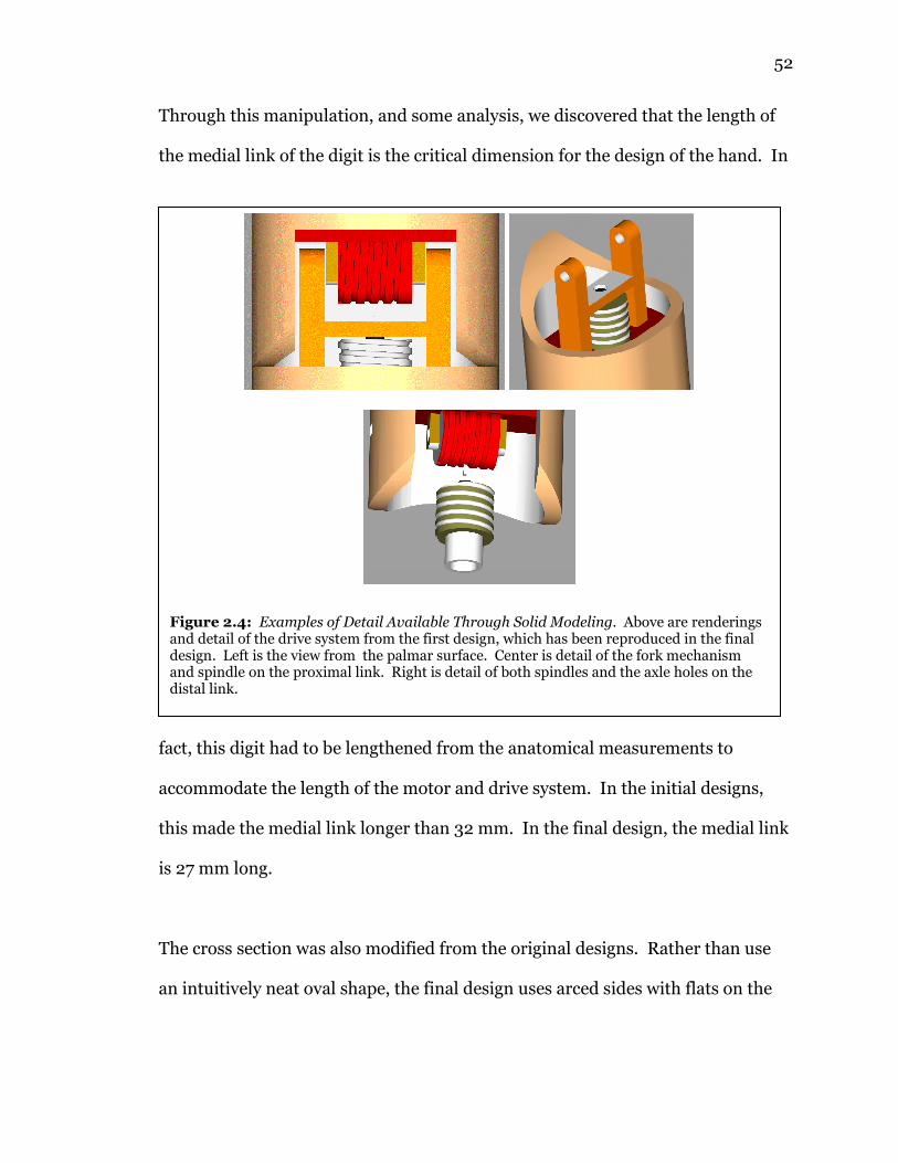
52
Through this manipulation, and some analysis, we discovered that the length of
the medial link of the digit is the critical dimension for the design of the hand. In
fact, this digit had to be lengthened from the anatomical measurements to
accommodate the length of the motor and drive system. In the initial designs,
this made the medial link longer than 32 mm. In the final design, the medial link
is 27 mm long.
The cross section was also modified from the original designs. Rather than use
an intuitively neat oval shape, the final design uses arced sides with flats on the
Figure 2.4: Examples of Detail Available Through Solid Modeling. Above are renderings and detail of the drive system from the first design, which has been reproduced in the final design. Left is the view from the palmar surface. Center is detail of the fork mechanism and spindle on the proximal link. Right is detail of both spindles and the axle holes on the distal link.

53
palmar and opposing surface. This more closely resembles the cross section of
the anatomical digit, with a wider palmar surface than top surface.
Once this new first digit design was complete, it was replicated with alterations to
the length of each link to form the phalanges. The cross sections of the digit were
not changed. Although the cross sections of the digits of the natural hand do vary
slightly, the cross section was reused to simplify design. The variations are so
small that the benefit from using identical cross sections outweighs the loss of
replication. Further extrusions to the distal link of each digit will make the tips of
the mechanical finger more rounded like a natural human finger.
2.2.2 Motors
The device itself, as well as the kinetic models discussed below, is driven by
Solarbotics geared DC motors manufactured by Sanyo. These motors are
sufficiently small to fit inside the shaft of the modeled digit, yet strong enough to
provide up to 800 g-cm (or 7.84 N-cm) of torque. In addition, a higher torque
model, the GM-14a with nearly 5 times the torque of the GM11 is available from
Solarbotics. Both motors have the same outline and dimensions. The GM11 was
used for the distal joint, while the GM14a motors were used for the other joints.
Although the complete transfer function of the motor could not be found from
measurements alone, approximations can be used to determine an estimate of
the motor transfer function. The motor torque constant, armature resistance,

54
and damping constant are specified by the manufacturer on their data sheet.
This allows for a partial determination of the time constant for the motor.
The generic transfer function of a DC motor is well known and given by several
sources, including Phillips and Nagle (1995). A DC motor exhibits an exponential
rise in speed, meaning it can be fully
characterized by a time constant alone, if the
inductance of the armature can be considered
negligable. Obtaining position from this transfer
function is done through simple integration, or
multiplication by 1/s in the Laplace domain. For
both speed and position, the motor can be completely described by a time
constant. The formula for this time constant is
BTa
a
KKBR
JR
+=τ
where J is the total rotational inertia, B is the total damping due to friction, Ra is
the armature resistance, KT is the motor’s torque constant, and KB is the motor
damping constant (which converts speed to torque based on motor
characteristics). Calculations yield an approximate time constant of 16.3
milliseconds, without load or significant drag (i.e. a free turning motor). As can
be seen from the formula for the time constant, the total rotational inertia and
damping friction are significant factors in the calculation. These values have not
been empirically determined for our model.
Figure 2.5: The Sanyo 12GN-0348 geared DC motor. Type NA1S has 76:1 reduction.

55
2.2.3 Sensor Tests and Physical Model
A kinetic model was developed in Mechanical Desktop and then fabricated using
Fused Deposition Modeling (FDM). These parts are self similar links in a system,
making fabrication very straight forward and efficient. Using a motor to drive the
rotation of the model, and a Hall Effect sensor to track the position allowed the
demonstration of motor control.
The single joint FDM kinetic model (discussed further below) has a range of
motion of 120 degrees. The digital acquisition values range from 130 to 170 with
8-bit A/D conversion. These digital values can be proportionally aligned to
analog values. Viewing the digital values as a linear quantization of the supply
voltage, calculations show that the theoretical output voltage range from the
sensor is 2.549V to 3.334V. Observations of the sensor output voltage showed a
range of 2.427V to 3.134V, indicating a non-linearity in the A/D converter. This
non-linearity is possibly a constant offset intrinsic to the sensor. It has not
impacted the ability to control the system.
Figure 2.6: Kinetic model for testing the control system. Left is a side view, center is a top view, right is detail of the Hall Effect sensor. The Hall Effect magnet is the brown circle, the small SIP package is the sensor itself.

56
2.2.4 Embedded Platform Single Joint Control
Fundamentally, the problem at hand is one of replication. The ability to control
one joint is central to the control of the entire device. A USB-enabled
microcontroller, specifically a PIC18F4550, was programmed to control a single
motor. A Hall Effect sensor provided an analog angular position signal, while a
pulse-width modulation (PWM) module was used for motor drive.
The processor was programmed for
two modes of operation: constant
velocity drive and proportional
feedback control. The constant
velocity drive moved the joint to
the desired angular position and
then stopped. The proportional
feedback control used a traditional
feedback, where the drive signal
was generated through proportional amplification of the error signal.
Control commands were provided by a C++ program running on a laptop (Dell
Latitude D620, Core Duo Processor, 512MB Ram). The laptop communicated via
USB to command the PIC18F4550 to control the motor in a specified way. The
PIC processor then recorded 1 second of data, sampled at 180Hz (determined by
calculation). This sampling rate was specified by setting an internal timer’s width
(in bits) and the associated prescaling hardware to cause an overflow 180 times
0 20 40 60 80 100 1202.4
2.5
2.6
2.7
2.8
2.9
3
3.1
3.2
3.3
Hall Effect Sensor Linearity
Position (degrees)
Sensor Output (Volts)
Observed
Calculated
Figure 2.7: Hall Effect sensor linearity. Top line is theoretical output, bottom line is observed voltage.

57
per second. Upon overflow, a hardware flag is set by the processor. Then, on the
next program loop, a conditional statement branches the program to store a data
point. Polling in this way, rather than interrupting the program on each timer
overflow, does lead to a potential variation in the sample rate. However, the
potential variation is much smaller than the sample interval, and can be assumed
to be negligible.
Each data point was the MSB of the A/D conversion result (the PIC18F4550 has
10-bit A/D resolution; the two LSbs were ignored). This 180 byte array was then
retrieved by the laptop for plotting and analysis. Upon the user’s USB command,
the processor, using the Microchip USB framework, packages the data into a
standardized packet (covered below in 2.2.6). A USB-standard ping-pong
communication protocol is used to return the data, ensuring no collisions occur
and the data is not corrupted. Three such packets are used to transfer all 180
bytes of data. The PC then stores the data in a text file, for later plotting and
analysis.
In both cases, data was collected, converted from digital values to real position
values (in degrees) by scaling the A/D result based on the observed positions.
Using linear interpolation, defining the clockwise-most position as 0 degrees, and
the counterclockwise most position as a maximum, the corresponding A/D
results are used as the scaling parameters. The data were then digitally filtered at
45Hz. This was done through a 16 tap low pass FIR filter specified by MATLAB
function 'fir1’ with cutoff frequency 0.5π, where π is the Nyquist Rate, or one

58
half of the sampling rate. While ‘fir1’ has a windowing option to reduce
stopband ripple, no windowing function was used.
The filter values were then
zero padded out to the
length of the data, and
filtering was performed
using FFT multiplication.
The first 25 points of the
filtered data were zeroed to
compensate for filter “start
up” effects and the phase
shift of the filter. Using an FIR filter limited distortion because FIR filters
generated by fir1 are RCSR-GLP: Real Causal Stable Reversible with
Generalized Linear Phase (Porat, 1997). The linear phase shift can be seen by
observing the x-axis shift of noise around 60 degrees at times 0.2sec and 0.35sec.
Prior to filtering, in all cases the signal to noise ratio was at or below -60dB.
0 0.1 0.2 0.3 0.4 0.5 0.6 0.7 0.8 0.9 10
20
40
60
80
100
120
140
time (seconds)
position (degrees)
Comparison of Fitlered and Unfiltered Data, Proportional Control (Kp = 24)
Raw Data
Filtered Data
Figure 2.8: The Effect of Filtering Data. Line to the left is unfiltered, line to the right is filtered. Note the linear phase shift.

59
0 0.2 0.4 0.6 0.8 10
20
40
60
80
100
120
Constant Velocity Data (Raw)
Time (seconds)
Position (degrees)
105
110
120
130
140
160
180
0 0.2 0.4 0.6 0.8 10
20
40
60
80
100
120
Constant Velocity Data (Filtered)
Time (seconds)
Position (degrees)
105
110
120
130
140
160
180
Figure 2.9: Constant Velocity data plots. Left is unfiltered raw data, right is filtered data with the first 25 data points removed for clarity. Legend at right shows digital values of drive.

60
0 0.2 0.4 0.6 0.8 1-20
0
20
40
60
80
100
120
Time (seconds)
Position (degrees)
Proportional Control Data (Raw)
k16
k20
k30
k50
0 0.2 0.4 0.6 0.8 1-20
0
20
40
60
80
100
120
Time (seconds)
Position (degrees)
Proportional Control Data (Filtered)
k16
k20
k30
k50
Figure 2.10: Proportional Feedback Gain Plots. Left is unfiltered raw data, right is filtered data with the first 25 data points removed for clarity. Legends indicate values of Kp, the proportional gain constant.

61
2.2.5 Device Hardware Architecture
A single processor with the 20+ inputs necessary for controlling the proposed
device may exist. However, one also with 20+ PWM outputs probably does not.
This restriction, in addition to limitations on processing power, has lead to the
development of a distributed control method. The use of several processors for
the lower level feedback control, communicating through a central coordinating
processor allows for modularity of the control system. In addition, the use of
several smaller PIC18 series processors rather than one large processor helped to
reduce the cost of the control system hardware.
Another microcontroller made by Microchip, the PIC18F2431, does not have USB
functionality but does have sufficient A/D inputs and PWM outputs to control
three joints, or a single digit. Both the 2431 and 4550 have I2C modules. I2C is
shorthand for Inter-Integrated Circuit, a synchronous protocol for chip to chip
communication. It is a byte-wise method, sending 8 bits at a time. Microchip
also supplies framework code for interfacing with the I2C module.

62
The goal is to make the system expandable without a complete rewiring of the
circuitry or complete reprogramming of every processor. Using a bus method,
like I2C, allows additional processors to be added with minimal wiring (the new
processor just needs to be hooked up to the existing bus) and minimal
reprogramming (only the master processor’s program needs to be updated).
The device is controlled by several processors coordinating and communicating
over the I2C bus. Each section of the hand, a finger in this instance, is controlled
by its own local processor. These local processors receive position data from a
central coordinating processor. The central coordinating processor handles the
“high level control” or “task level control” spoken of above. Commands can also
be fed to the coordinating processor over USB from a PC or other suitable USB-
enabled device.
USB Interface
I2C Interface
PC USB
I2C Bus
Embed
ded
Contro
llers I2C Slaves
PIC 18F4550 I2C Master, USB device
Figure 2-11: Block Diagram of hardware (rectangles) and software (ovals) architecture.

63
2.2.6 Software Architecture
The software for the system is broken down into several modules, so each can be
assigned to an appropriate processor when the above described distributed
architecture is implemented. Though the ANSI C language does not have classes,
like C++ does, an object-oriented approach can still be taken using separate
functions for each major section of the system.
Figure 2.12: An overview of the controller test platform. To the left is the kinetic model discussed above, with motor, hall effect sensor, and supports. In the center is a breadboard. The long chip toward the top is a PIC18F2431. The bottom half of the breadboard is a PWM motor driver (On the red PCB) , a buffer, and a header to interface with the development board. On the right is the PIC18F4550 full-speed USB development board. The processor itself is under the grey ribbon cable. The smaller grey ribbon cable running from the development board to the PIC18F2431 is the I2C bus. On the far right is the USB cable to the commanding PC. At the back is the DC power supply for motor drive.
Embedded Controller I2C Slave
PWM Motor Driver
I2C Bus
USB to PC
Coordinating Processor w/USB I2C Master
Controlled Plant: Motor and Sensor

64
As mentioned above, this device is a multi-processor system. The programs for
the coordinating processor and the slave (or local) processors are markedly
different, because the purpose of each processor is different. However, each of
the local processors has essentially the same program architecture. This is not to
say that the programs are identical, however, as joint and controller specific
information will be altered for each processor. Further, there is host software on
the PC that allows interfacing with the device.
Each of the microcontrollers is programmed using Microchip’s MPLAB
development environment and either a USB-based programmer or Microchip’s
ICD2 In Circuit Debugger and Programmer. Microchip also supplies the
compiler, linker, I2C firmware and USB firmware.
2.2.6.1 Analog-to-Digital Conversion
For all of the Microchip embedded processors used herein, user configured
timers are used for ADC conversion control and other timed operations, such as
the LED indicators and motor drive time out. The ADC conversion method is a
modification of code developed by Space Exploration Technologies’ Senior
Avionics Engineer R. Kevin Watson (Watson, 2008) (used with permission).
Motor drive is calculated using a proportional feedback control method, and
output values are updated asynchronously with respect to ADC conversions. This
is possible due to buffering of the ADC result provided by Watson’s code.

65
2.2.6.2 Coordinating Processor Software Architecture
There are three (3) major sections of the coordination program:
(a) An interface method for communicating with the PC.
(b) A maintenance process.
(c) A communications method for the I2C bus.
The program centers around an infinite while loop, a common programming
convention for microcontrollers. Each time through the loop a set of three
functions is called.
First, the USB bus status is checked. If there is information waiting on the bus, it
is handled. The processor updates its internal information based on information
received over USB. The USB information can include position and response
information for one or more processors, or a direct I2C command to be sent to a
particular device.
Second, the maintenance process is performed. This performs any parsing,
calculation, or other method mandated by the current or previous data received
by the processor over USB. Also, if necessary, this function updates data in the
processor.
Third, if needed, an I2C handling function distributes information to each of the
low level processors. Again, if necessary, the processor’s data is updated.

66
From instance to instance of the while loop, global variables are used to hold data
and parameters that would otherwise be lost when a function returned or another
instance of the loop was initiated. These variables include I2C read and write
buffers, indices for arrays, previous position values, etc. These structures can be
considered an abstract state of the processor.
2.2.6.3 Embedded (Local) Controller Software
The several slave processors on the I2C bus could be referred to as slave
processors, embedded controllers, or local controllers. Regardless of the
terminology, these are the terminal processors that drive the actuators of the
device.
These processors share many features of the coordinating processor, but also
have additional modules for motor control. They use the infinite while loop
Figure 2.13: Block Diagram of Coordinating Processor’s Software
USB Handler
Maint. Process
I2C Handler
Abstract State
I2C Hardware
USB Hardware
I2C Bus
USB Bus
while(1) loop

67
described for the coordinating processor. However, they do not have USB
functionality and they are slaves on the I2C bus. In addition, they hold
information for the kinetic models of the systems they control, use analog to
digital (A/D) conversion modules, and pulse width modulation (PWM) modules.
Like the coordinating processor, the program is divided into two functions: one to
handle the I2C communication, and another to handle the motor control. For
these processors, the abstract state is the desired positions, control method, and
any previous pertinent control information (the last state in a state space model,
for instance) for each motor.
I2C is handled by interrupt. The I2C hardware determines if there is an I2C
request for that particular processor’s address. If the address for the request and
the processor’s address match, a processor interrupt occurs, which calls a
Figure 2.14: Block Diagram of Embedded Controller Software
I2C Handler
Motor Handler
Abstract State
I2C Slave
Module I2C Bus
while(1) loop
PWM
A/D
Control Information:
(a) PID Gains
(b) State Space Observer/Controller
Kinetic Model
Sensors
Motors

68
handling function. The handling function reads the data off the bus, stores it in a
buffer, and changes the state of a flag to indicate that new data has been received.
The motor handler reads the abstract state to determine the desired position and
other control information. This position is compared with a new A/D sample. If
an error exists, a drive signal is produced using a control method. This drive
signal is then passed to the PWM module for output to the motor. The PWM
module continues generating output based on the duty cycle value stored in the
PWM registers between loop instances, so constant updating is not necessary.
This method is repeated for each motor the processor controls
2.2.6.4 USB Packet Structure
The Microchip USB module meets the USB 2.0 specification, and uses a “ping-
pong buffer” with 64 byte packets. The first four of the bytes in the custom
packet for this project contain the packet command, packet type, packet number,
and packet length. The packet length is used as a checksum to verify a complete
transmission. The bytes following these four common bytes hold data up to 60
bytes in length per packet. For control of the device, commands for up to 20
actuators can be sent in a single packet.
Command Type ID length DATA (60 bytes) 0 1 2 3 4 64
Figure 2.15: USB Packet Structure. Numbers indicate byte index.

69
2.2.6.5 Host Computer Software
In addition to the device programming, the controlling host is currently a PC with
a program developed using C#.NET. This program handles all the commanded
test inputs to the device, the USB communication, and data retrieval functions.
Using the .NET Framework allows the development of a smooth neat efficient
application with clean user interface. Further, .NET has methods to load DLL
files, write to files, and produce clean professional looking windows for the UI.
The host program is far more complex than the controller programs. Thankfully,
it is simpler to program because Microsoft Visual Studio automates the
generation of many files and functions, so little alteration is necessary. Also,
Microchip provides a USB driver and interface library, so extensive low-level USB
programming is not necessary.
The host program is, in large part, a conversion method, taking the byte stream
that enters over USB and converting it to usable types in the host controller.
Each USB packet is parsed, and functions are called based on the information in
the USB packet. Also, the user interface allows input by an experimenter. These
inputs are translated into USB packets for transmission to the controller(s).
Further advantages are gained using C++/C# rather than C on the PC. Since the
application has been developed on C++/C#.NET, the Microsoft .NET framework
provides common language runtime, allowing future cross-language development

70
in Visual Basic, C++, C#, and J#. Also, C++.NET supports SQL queries on both
Microsoft SQL and MySQL. This opens possibilities for database support, web-
based interaction, and further development by other researchers after the project
is complete.
The ideal situation, however, is one where the host used here is an embedded
USB-enabled processor. This would make the device fully mobile, and a more
effective prosthesis system. The PC serves as a placeholder for this embedded
processor, which detects the user’s volition. Such a system is outside the scope of
this project.
2.3 Mechanical Assembly
Following some aesthetic modification of the above mentioned digit design,
including rounding of the finger tips, several sets of the four links required for
Figure 2.16: Block Diagram of Embedded Controller Software. Notations on arrows indicate types being passed. No notation indicates function call.
USB DLL USB Handler
User Interface
USB Bus Ctrl USB Bus
Logging Handler
Packet Processor / Parser
Files
Action Handler
byte[] char[]
ostringstream
ofstream
cin/cout CEvent

71
each digit were produced using Fused Deposition Modeling (FDM) through the
Rutgers University Mechanical Engineering Department.
Due to characteristics of the FDM process, several post-fabrication modifications
were necessary. Principal among these was a failure to account for the width of
the FDM filament. This resulted in an undersizing of all inside dimensions by
approximately 0.5mm.
Holes for axles were drilled out using a 2.1mm drill using a Bridgeport Mill, along
with necessary shims, vices, etc. Internal faces of the hinge joints were similarly
machined on the mill, using a small end mill. Cavities for the motor and gearbox
were adjusted using a Dremel tool with the appropriate bit, as well as small round
and square files.
2.3.1 Novel Method for Right Angle Transmission
One key hurdle to overcome is the right angle transmission of motion from the
motor, which is con-axial with the shaft of the digit, to the axis of rotation, which
is perpendicular to the shaft of the digit. While bevel or worm gears could be
used to accomplish this, a test platform for an experimental wire-driven system
was designed and fabricated. This design has several advantages, including low
failure cost and mechanical compliance. The low failure cost is due to the use of
low cost steel wire for the transmission mechanism. This wire also provides
mechanical compliance, meaning that driving the system backwards will not
necessarily cause damage to the transmission. Following preliminary testing

72
using the experimental platform, suitable parts were made for use in the finger
itself.
2.3.1.1 Application to Joint Drive
One end of the transmission, the output spindle for rotation of the joint, is
integrated into the link and fabricated by FDM, however, an input to the
transmission is not created in this step. Therefore, a suitable method for
mounting a spindle on the motor output shaft was necessary.
For this part of the transmission, steel threaded rod (1/4”-20) was used for the
spindle. The rod was trimmed to 1cm length using a band saw followed by a
metalworking lathe. After the part was trimmed, a 1/8” hole was drilled down the
axis of the rod to accommodate the motor shaft. A hole was then drilled through
the side of the rod, and tapped for a #4-40 setscrew. This setscrew secured the
rod on the motor shaft by contacting the flat on the motor shaft.
Figure 2.17: Pictures of the test bed (large white object) and miniaturized design (smaller yellow translucent object. Diameter of the large spindles is 1cm, the small spindles are 6mm.

73
2.3.1.2 Transmission Assembly
Following the mounting of the drive spindle to the motor, adjacent links were
connected using 2mm diameter stainless steel dowels. These dowels were
pressed into the ABS plastic in each link to secure the axis of rotation. The end of
this dowel could be
secured using Loctite
480 adhesive,
however, this step
was not taken during
the testing phase.
Prior to the insertion
of the stainless steel
dowel, 24ga nylon-
coated steel wire was wrapped around the spindle of the distal link. This wire
was then wrapped around the steel spindle mounted to the shaft of the motor in
the proximal link. Following a settling period of 12-24 hours to relax the wire and
give it “memory”, the nylon near the intersection of the two ends of the wire was
melted using a soldering iron. These sites were then cleaned using soldering flux,
and were realigned on the spindle. The ends of the steel wire were then joined
using solder, and the loose ends removed. This completed assembly of the
transmission.
Figure 2-18: A digit joint in the assembly jig.
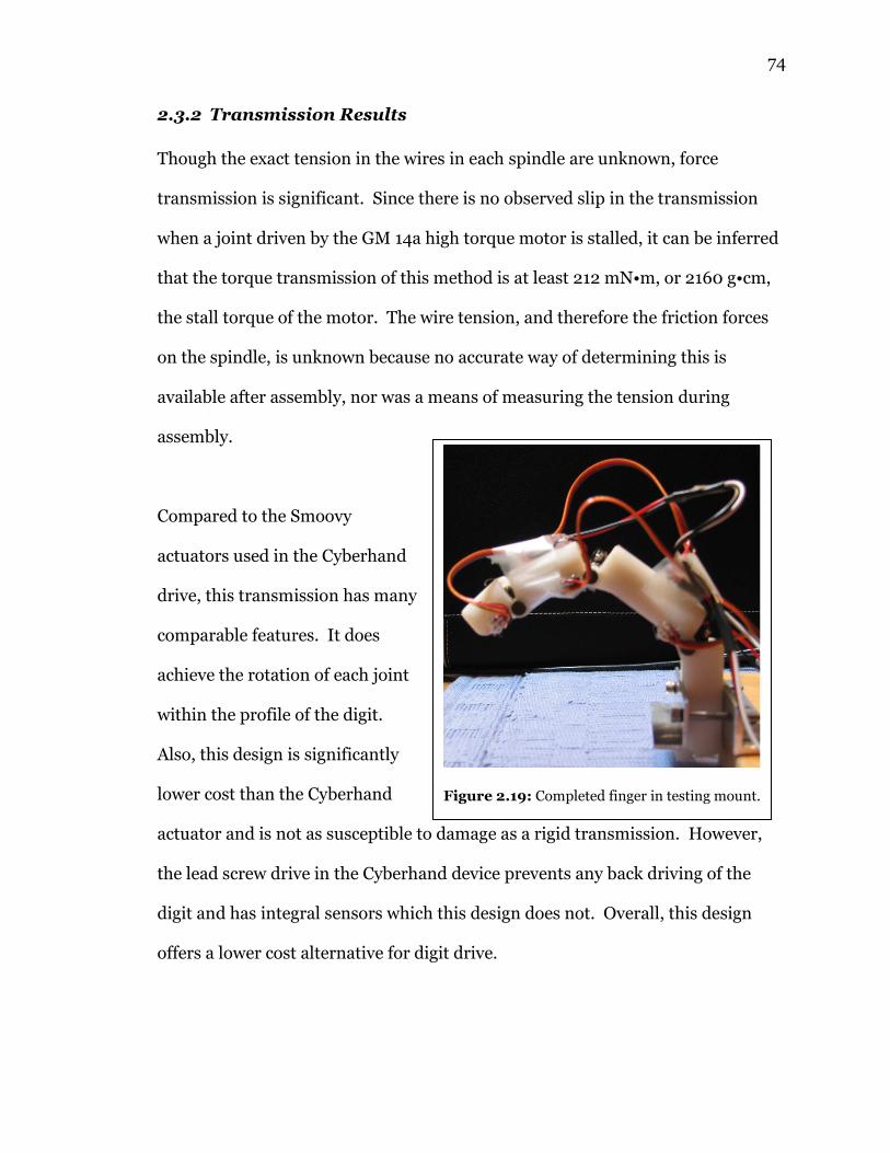
74
2.3.2 Transmission Results
Though the exact tension in the wires in each spindle are unknown, force
transmission is significant. Since there is no observed slip in the transmission
when a joint driven by the GM 14a high torque motor is stalled, it can be inferred
that the torque transmission of this method is at least 212 mN•m, or 2160 g•cm,
the stall torque of the motor. The wire tension, and therefore the friction forces
on the spindle, is unknown because no accurate way of determining this is
available after assembly, nor was a means of measuring the tension during
assembly.
Compared to the Smoovy
actuators used in the Cyberhand
drive, this transmission has many
comparable features. It does
achieve the rotation of each joint
within the profile of the digit.
Also, this design is significantly
lower cost than the Cyberhand
actuator and is not as susceptible to damage as a rigid transmission. However,
the lead screw drive in the Cyberhand device prevents any back driving of the
digit and has integral sensors which this design does not. Overall, this design
offers a lower cost alternative for digit drive.
Figure 2.19: Completed finger in testing mount.

75
2.3.3 Mounting of Position Sensors
Position feedback from the joints is provided by Hall Effect sensors, Allegro
Microsytems model A1301. These small integrated circuits are mounted next to
magnets (provided by Dexter Magnetic Technologies), polarized to detect the
position of the joint, and convert the magnetic field intensity to voltage, for
reading by the processor’s ADC channels. The Hall Effect magnet was mounted
in a cylindrical mounting hole, produced during FDM, and secured with hot glue.
The Hall Effect Sensor IC was similarly mounted next to the magnet, and
similarly secured with hot glue.
The polarization of the magnets is radial rather than the more common axial
polarization. This means that the left hemi-cylinder of the magnet is one pole,
and the right hemi-cylinder is the other pole. Therefore, the intensity of the
magnetic field at a fixed point near the magnet changes with rotation of the
magnet about its axis. It is this change that the Hall Effect sensor detects and
converts to voltage. The voltage is then related to position in the processor.
2.4 Electronic Hardware Platform
For the control system approach, a networked modular method was preferred,
using several slave processors for local control, coupled with a master processor
with higher computational power for coordination and intelligent control. These
several processors are networked via the Inter-Integrated Circuit (I2C) bus. In
addition, the master processor has Universal Serial Bus capability. These two

76
busses allow for extensibility of this architecture to applications beyond
prostheses.
2.4.1 Local Processing
In this application, a Microchip PIC18F2431 processor for embedded applications
is used to control each digit. The processor has 5 pulse-width-modulated (PWM)
outputs for motor drive, and 5 analog-to-digital conversion (ADC) channels for
sensor feedback (Microchip, 2008). As previously mentioned, each processor
also has an I2C module for communication. For diagnostic purposes, two light
emitting diodes each with 2N7000 MOSFET driver allow for visual indication of
the processor’s operating state.
Pulse Width Modulated (PWM) signals are used to control the motors. The input
voltage to the motor determines the motor speed. However, in order to specify a
range of voltages at resolution necessary to control the digit, a wide (8-bit or
more) digital to analog converter would be necessary. This would require many
processor pins, and may not have current capacity necessary to drive the motor at
stall.
To reduce the number of output pins necessary on the processor, most embedded
processors use PWM to communicate output voltage. If the time constant of the
motor is significantly longer than the PWM pulse interval, then the motor
behaves as a low pass filter on the PWM signal. Then, the width of the PWM
pulse becomes the determining factor in motor voltage, since the motor’s low

77
pass characteristics essentially smooth the pulse train into a relatively constant
voltage, and hence a constant speed.
Processor pin current ratings are generally low. The PWM signal from the
processor does not directly power the motor. Rather, motor driver circuitry
receives the PWM signal. These drivers allow the motors to draw their current
directly from a power supply, bypassing the processor. This means that motor
power is independent of the processor, and relies on the power supply, and the
wiring between the motor and the power supply. Also, it means that a given
processor can drive and control different motor loads, so long as the driver
circuitry is able to supply the current necessary for the load. Specifically for this
project, L293D motor drivers, available in chip form from ST Microelectronics
(ST Microelectronics, 2008) or on an application board from Solarbotics
(Solarbotics, 2008), are used to provide power to the motor.
2.4.2 Electrical Characteristics and Board Design
This modular finger actuator is capable of delivering 16 W of electrical power at
peak usage, 275 mW of which powers the processor. The actuator itself achieves
the expected full range of motion. The processor operates with a clock speed of
20 MHz, running at half its rated 40 MHz speed. This oscillator was chosen
partially due to availability of parts and partly to reduce power consumption.
Though underclocked, the processor is capable of the sensing, feedback control,
and PWM drive generation without processing delays.
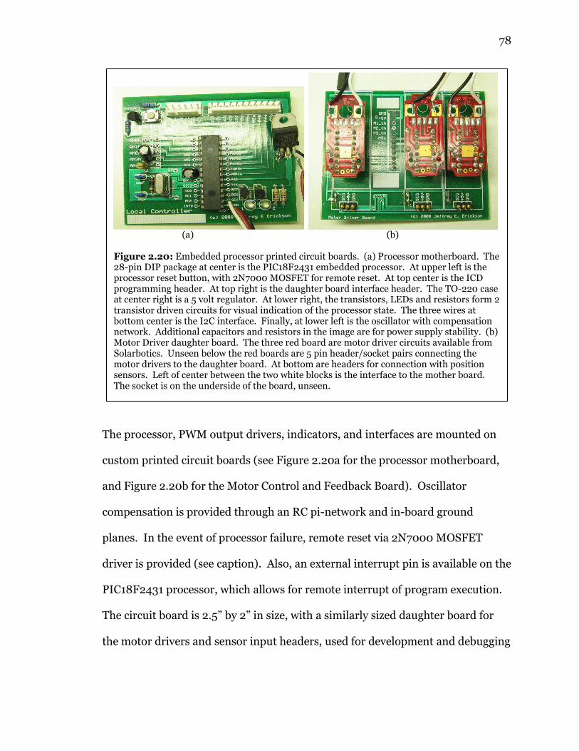
78
The processor, PWM output drivers, indicators, and interfaces are mounted on
custom printed circuit boards (see Figure 2.20a for the processor motherboard,
and Figure 2.20b for the Motor Control and Feedback Board). Oscillator
compensation is provided through an RC pi-network and in-board ground
planes. In the event of processor failure, remote reset via 2N7000 MOSFET
driver is provided (see caption). Also, an external interrupt pin is available on the
PIC18F2431 processor, which allows for remote interrupt of program execution.
The circuit board is 2.5” by 2” in size, with a similarly sized daughter board for
the motor drivers and sensor input headers, used for development and debugging
(a) (b)
Figure 2.20: Embedded processor printed circuit boards. (a) Processor motherboard. The 28-pin DIP package at center is the PIC18F2431 embedded processor. At upper left is the processor reset button, with 2N7000 MOSFET for remote reset. At top center is the ICD programming header. At top right is the daughter board interface header. The TO-220 case at center right is a 5 volt regulator. At lower right, the transistors, LEDs and resistors form 2 transistor driven circuits for visual indication of the processor state. The three wires at bottom center is the I2C interface. Finally, at lower left is the oscillator with compensation network. Additional capacitors and resistors in the image are for power supply stability. (b) Motor Driver daughter board. The three red board are motor driver circuits available from Solarbotics. Unseen below the red boards are 5 pin header/socket pairs connecting the motor drivers to the daughter board. At bottom are headers for connection with position sensors. Left of center between the two white blocks is the interface to the mother board. The socket is on the underside of the board, unseen.
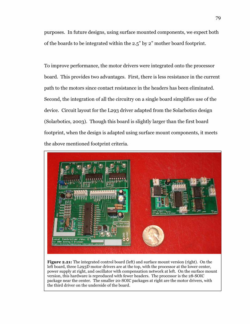
79
purposes. In future designs, using surface mounted components, we expect both
of the boards to be integrated within the 2.5” by 2” mother board footprint.
To improve performance, the motor drivers were integrated onto the processor
board. This provides two advantages. First, there is less resistance in the current
path to the motors since contact resistance in the headers has been eliminated.
Second, the integration of all the circuitry on a single board simplifies use of the
device. Circuit layout for the L293 driver adapted from the Solarbotics design
(Solarbotics, 2003). Though this board is slightly larger than the first board
footprint, when the design is adapted using surface mount components, it meets
the above mentioned footprint criteria.
Figure 2.21: The integrated control board (left) and surface mount version (right). On the left board, three L293D motor drivers are at the top, with the processor at the lower center, power supply at right, and oscillator with compensation network at left. On the surface mount version, this hardware is reproduced with fewer headers. The processor is the 28-SOIC package near the center. The smaller 20-SOIC packages at right are the motor drivers, with the third driver on the underside of the board.

80
Figure 2.21 shows the results with the two integrated controller boards. The two
boards are functionally identical. The large scale DIP package board was
produced with indicator lights and the 12 pin header from the non-integrated
version. The surface mount version does not have the indicator lights, but uses
an identical processor in a surface mount package. To conserve space, a motor
driver is located on the underside of the board. In this configuration, the
circuitry is sized to fit inside a potential prosthesis, either in the forearm portion
or in the palm.
2.4.2.1 Supervisory High Level Processor
The high level processor is a PIC18F4550 on a Microchip supplied development
board. Like the PIC18F2431, this processor has an I2C module and acts as the
master controller on the bus. Also, this processor has a USB module for
communication with a USB host. Supervisory control that this processor
provides allows for the coordination of several of the processors in the modular
finger actuator mentioned above (Erickson, et al, 2007).

81
Chapter 3: Control Modeling
Rather than immediately implementing everything on the hardware, simulation
was used both to reduce costs and minimize the risk of damage. By developing a
model for the digit joint from the physics of the motor and joint, several versions
of the control methods can be evaluated with no additional hardware cost.
Ultimately, the algorithms tested in simulation would be implemented on the
embedded controller described above.
Inherent in the control problem faced in development of a manipulator for
prosthetic purposes is the non-linearity of the system configuration. A system
with non-linearities presents several problems when designing a controller.
First, in many cases, use of linear control methods with a non-linear system tend
to yield less than satisfactory results. Second, if a linear control method is used
and can control the system, this tends to apply only to a small set of conditions,
such as a limited range of motion. Third, if some non-linear control approach is
used, the stability of the system must be scrutinized not only for the short term
dynamics, but for long term stability at the target position.
3.1 Single Joint Control Model
To study potential approaches to the aforementioned control problem, a
mathematical model of the single joint was developed for use in computer
simulation. This model was derived from the equations of motion for the joint,
simplified to a point mass rotating about a center of rotation. The DC motor used

82
as the actuator was also modeled, with values based on the manufacturer’s data
sheet as well as laboratory measurements. Following this first pass at model
extraction, verification was attained by running the simulation as a free turning
frictionless motor.
3.1.1 Derivation of the Equations of Motion
Viewing the single joint as a sum of all torques about the center of rotation, there
are four terms that appear in the balance of torques:
(3.1)
First, the rotational inertia term is expressed as the moment of inertia times the
angular acceleration:
(3.2)
The moment of inertia was calculated assuming a point mass equivalent to the
weight of the arm being rotated at a radial distance one half the length of the arm.
Second, the kinematic or dynamic friction
term is expressed as a friction coefficient
times the angular velocity:
(3.3)
This friction coefficient is a constant
chosen based on assumptions of the
materials and construction of the joint.
∑ =−++ 0: mgbJ τττττ
θτ &&JJ =
θτ &bb =
M
Fg bω
rmg•sinθ
Jα
Figure 3.1: Schematic of forces and inertial acting on the single joint. Inertia is Jα, friction force is bω, force due to gravity is Fg, and torque due to gravity is rmg•sinθ.

83
Third, the torque due to gravity is the dot product of the force due to gravity (mg)
with the horizontal distance to the center of rotation (r sin θ):
(3.4)
Finally, the fourth term is motor torque, expressed as a transmission constant
times the torque generated by the motor:
(3.5)
Combining equations 3.1 through 3.5 yields a non-linear differential equation
governing the model system:
(3.6)
3.1.2 Extraction of the DC Motor Model
The standard model for a brushless
DC motor applies to the miniature
motors used as the actuators.
Modeling the motor requires the
description of essentially two
separate systems.
The time course of current given an applied voltage is modeled as an LR circuit.
Values for the inductance and resistance were measured using an HP 4284A
precision LCR meter (see table 3.1). The meter was calibrated using an open
circuit before operation, and used a 1kHz sinusoid with no DC bias as the input to
the motor. During testing, all values observed were steady and no rotation or
vibration of the motor was noted.
Table 3.1: Motor Electrical Characteristics
Motor Type Inductance Resistance GM11 (Low Torque)
2.81 mH 20.1 Ω
GM14a (High Torque)
2.09 mH 12.90 Ω
)sin(θτ rmgg =
motorm kττ =
motorkrmgbJ τθθθτ =++∑ )sin(: &&&

84
Output torque of the motor can be expressed as proportional to the current
through the motor. The proportionality constant is the motor’s torque constant,
which relates the motor torque to motor current, and is denoted below as Kτ.
The value of this constant is calculated by dividing the stall torque by the short
circuit current, as specified on the manufacturer’s data sheet.
Therefore, the torque generated by the motor is:
(3.7)
Where Kτ is the motor torque constant, calculated as described above, and
evaluated to be 0.4 N•m/A.
The internal dynamics of the motor are modeled as an RL circuit, using the
inductance and resistance at the motor terminals, with values given in Table 3.1.
The input is the voltage applied to the motor terminals:
(3.8)
This differential equation relates the time course of current to the applied
voltage. Current response is not instantaneous due to effects of the motor’s
magnetic field. Starting with a stopped shaft, energy must be put into the
magnetic field as the shaft begins to turn. After the shaft is turning, the magnetic
field induces electromotive force (EMF), which limits the rate of change of
current. This induced EMF also appears as a voltage across the coil, which is
iKmotor ττ =
appliedVRidt
diL =+

85
subtracted from the terminal voltage to give the applied voltage mentioned in
equation 3.8:
(3.9)
The back EMF voltage can be expressed as a constant times the motor shaft
speed:
(3.10)
The constant, Ke, determines the motor’s free-running speed for a given voltage.
By inspecting equations 3.9 and 3.10, it can be seen at a certain speed, the back
EMF will equal the terminal voltage. That shaft speed is the free-running speed
of the motor. Calculation of this value began with an estimate, found by dividing
the free running back EMF by the manufacturer’s specified free-running speed.
The free-running voltage was found by multiplying the motor resistance,
measured above, by the motor’s rated free-running current, specified by the
manufacturer. This yielded a back EMF constant of 0.717 V•s/rad.
Combining equations 3.9 and 3.10 yields a differential equation for applied
voltage:
(3.11)
Substituting this result into equation 3.8 yields:
(3.12)
EMFtermapplied VVV −=
θ&eEMF KV =
θ&etermapplied KVV −=
θ&eterm KVRidt
diL −=+

86
Sum of Torques
Acceleration
Velocity
Position
Torque due to Gravity
Coil Voltage
Theta _dot _dot
3
Theta _dot
2
Th
1
rmg
-K-
radians to degrees
-K-
Torque Constant
0.4
Subtract
Motor Inductance
1
0.00209 s+12.90
Moment of Inerita
1/(4*10^-4)
Integrator 2
1
s
Integrator 1
1
s
Friction
-K-Dot Product
sin
Back EMF
-K-
0 to 90 degree limit
Vin
1
Figure 3.2: Simulink Model of the DC Motor. At upper left is Vin, the voltage applied to the terminals. The back EMF is subtracted from this, and the result is used as the input to an RL network. The resulting current is then multiplied by the motor torque constant and fed to the sum of torques. The result of the sum of torques is divided by J, the inertia, to yield the angular acceleration. The angular acceleration is then integrated to calculate angular velocity, and again for angular position. Angular position is fed back to the sum of torques as a term in the torque due to gravity. Angular velocity is fed back to the sum of torques via the friction term, and is also used to calculate back EMF.
3.1.3 Model Implementation and Verification
Using MATLAB with Simulink, this model has been implemented by summing all
torques to calculate the torque influencing the rotation of the arm. This result is
divided by the rotational moment of inertia to find the angular acceleration.
Integrating the angular acceleration yields the angular velocity, and integrating
angular velocity yields angular position. These intermediate values are used for
calculation of the friction and torque due to gravity terms, as well as the back
EMF of the motor.

87
-0.2 -0.1 0 0.1 0.2 0.3 0.4 0.5 0.6 0.7 0.80
10
20
30
40
50
60
70
80DC Motor Model Verification
Time (seconds)
Position (degrees)
Figure 3.3: Output of DC Motor Model following adjustment of back EMF constant. The step input to supply voltage occurs at 0 seconds.
For determining the motor torque, the back EMF of the motor is calculated, as
mentioned. This voltage is subtracted from the motor terminal voltage, and the
result is the input to the RL model of the motor windings. Current is the result of
this RL model, and is multiplied by the motor torque constant to calculate the
output torque of the motor.
Verification of the model is performed using a free running case, and verifying
the motor steady state speed. As the angular velocity of the motor increases, the
back EMF increases, this
in turn decreases the
effective voltage applied
to the motor terminals.
This decreases current,
and hence torque, and
causes the motor to turn
at a constant steady state
speed. To simulate this,
the friction and torque
due to gravity terms
were removed from the model, leaving only the motor model and the (small)
rotational inertia. Calculation of the sum of torques, angular acceleration, and
angular velocity were performed as above. The first pass of verification yielded
an error in the steady state speed of the motor.

88
Following empirical trial and error adjustment of the motor back EMF constant
from 0.717 to 0.8115, the proper steady state velocity of 76 rpm at 6 volts, as
specified by the manufacturer’s data sheet, was attained. As noted above, in
equation 3.10, the motor’s back EMF constant is the determining factor for
steady state speed. Calculations based on the data sheet yielded the value of
0.717. However, simulation with this value yielded a steady state speed that was
higher than the manufacturer’s specification. Through trial and error, increasing
the value to 0.8115 yielded the proper steady state speed.
3.1.4 Commentary on the Non-Linearity
From the perspective of a single joint, the non-linearity caused by the
gravitational force on the lever arm needs to be accounted for. When the joint
moves from a horizontal to vertical angular position, the torque due to gravity
varies according to the sine of the angle relative to the horizontal. Since the sine
function is linear for much of this range of motion, the system behaves well with a
linear feedback control system.
This linearity can be shown algebraically. If approximated at 0, the linearization
of sine is a linear function with slope 1, since the derivative of sine at 0 is 1. The
y-intercept of this function is 0, since sine is 0 at the origin. Using these
formulae, we can define a percent linearity function:
(2.5.13)
100)sin(
)(sin ×−
=x
xxxL
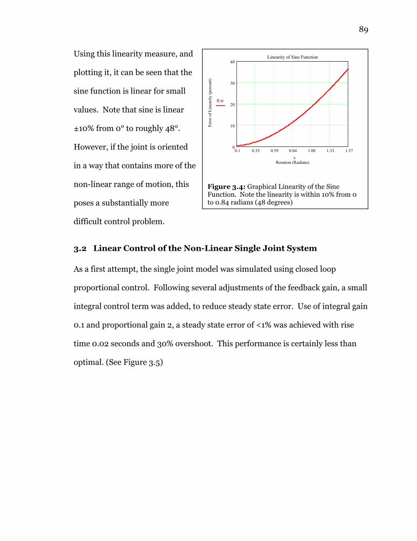
89
Using this linearity measure, and
plotting it, it can be seen that the
sine function is linear for small
values. Note that sine is linear
±10% from 0° to roughly 48°.
However, if the joint is oriented
in a way that contains more of the
non-linear range of motion, this
poses a substantially more
difficult control problem.
3.2 Linear Control of the Non-Linear Single Joint System
As a first attempt, the single joint model was simulated using closed loop
proportional control. Following several adjustments of the feedback gain, a small
integral control term was added, to reduce steady state error. Use of integral gain
0.1 and proportional gain 2, a steady state error of <1% was achieved with rise
time 0.02 seconds and 30% overshoot. This performance is certainly less than
optimal. (See Figure 3.5)
0.1 0.35 0.59 0.84 1.08 1.33 1.570
10
20
30
40Linearity of Sine Function
Rotation (Radians)
Error of Linearity (percent)
f x( )
x
Figure 3.4: Graphical Linearity of the Sine Function. Note the linearity is within 10% from 0 to 0.84 radians (48 degrees)

90
This demonstrates what control theory also shows: a non-linear system cannot be
controlled by a linear controller. This is not to state that for a bounded input to
the non-linear system that a linear controller will necessarily cause instability.
However, the control system performance parameters, like overshoot, rise time,
and steady state error, cannot be met using a linear controller on a non-linear
plant. Therefore, some non linear, time varying, or adaptive controller is
necessary to control a non-linear system reliably.
0 0.1 0.2 0.3 0.4 0.5 0.6 0.7 0.8 0.9 10
10
20
30
40
50
60
70
80
90
Time (seconds)
Position (degrees)
Linear and Non-Linear Response Comparison
Linear Response
Non-Linear Response
Figure 3.5: Model Trajectory Under Linear PI Feedback Control. The top (green) trace is the non-linear response, with increased overshoot and tracking error. The bottom (blue) trace is a linear response, substituting θ for sinθ. Both are in response to a step input at 0.2 seconds.

91
Reference Model
MR Out
2
System Position Out
1
Supply Limit
Subtract 1
SubtractStep
Scope 1
Scope
Product
Model
SingleJoint
Vin
Th
Th _dot
Th _2dot
MR Error GenerationLTI System
tf(100 ,[1 10 0 ])
Ki Gain
0.1
Integrator
1
s
Gain2
Constant
1
Add1
Add
Figure 4.1: Simulink model for MRAC. The ‘Single Joint’ block is the model from above, at upper left is the reference mode, with the indicated error calculation. Blocks near the center compute the control signals. The lower path is the integral path, which is static. The upper path multiplies the model reference error with the current system error, to implement MRAC.
Chapter 4: Model Reference Adaptive Control
Model Reference Adaptive Control (MRAC) was used as an adaptive non-linear
controller to solve the control problem. The MRAC approach uses a reference
model and compares the model response to the system (plant) response. The
instantaneous error between the model and plant is used as an adaptation
mechanism, altering the controller characteristics.
Use of MRAC requires the specification of the model to be tracked. An added
benefit of MRAC is the ability to specify the trajectory of the joint through the
model paramters. Returning to the whole hand scenario, many different paths
and speeds can be envisioned in the operation of the hand. For example, should
PI Controller
Reference Model
Model Reference
Error Generator

92
the hand respond quickly, as when snatching a bug, or slowly as when gripping a
soft object. Concieveably, this performance data could be specified by a position
time course for each joint. This, however, would require a great deal of
communication between controllers during operation of the hand. Alternatively,
the speed of the motor could be limited in software. Speed limiting would limit
the number of trajectories available.
By using MRAC, the trajectory is specified by the model. This means that the
trajectory information can be communicated as the model parameters. As a
result, rather than using hundreds of data points per second in the time course
approach, the MRAC approach would communicate similar information using
fewer than 10 numbers, depending on the order of the model used. All that
would need to be communicated are the coefficients of the model transfer
function and the target position.
The model response to be tracked was a second order system, implemented as an
integrated exponential impulse response with time constant 0.1 sec under unit
proportional feedback control. Further analysis of this model yields a second
order damped system with damping constant 0.5 and natural frequency 10
rad/sec. The model reference error was calculated as the difference between the
model response and the system response at each time point in the simulation.

93
For testing purposes, the system was implemented in Simulink, using the single
joint model from above as the plant. The input used is a variable amplitude step
function, with amplitude corresponding to degrees from horizontal.
System error is calculated by subtracting the system position value from this
target value. Error is then fed to a proportional-integral (PI) controller, which
generates the control signal for the plant. This control signal is limited to a user
specified supply voltage range before being sent to the input of the plant.
The input is additionally used as the input to a model system, which is under
unity proportional feedback control. This output is subtracted from the system
response at each time point to provide tracking error. Below, this error will be
referred to as MRAC error or MRAC tracking error.
4.1 With Linear Model Reference Error Feedback
This error was used to vary the proportional feedback control gain. This
adjustment caused an increase of the gain while the system lags the model, and a
decrease of the gain if the system leads the model. While this approach does
blunt the curve, preventing overshoot, if the gain is decreased enough, the
proportional gain becomes negative. When this occurs, the feedback control loop
becomes unstable, as established by feedback control theory. The observational
result in the simulation is a dip in the response as the model output becomes less
than the current system output.

94
The resulting response does
achieve acceptable model
tracking on the rising portion
of the response. This
demonstrates the
specification of trajectory via
specification of the reference
model parameters. However,
the instability which causes
the dip in response is less
than desireable. Also, the
ideal scenario would be proper tracking of the model continuously throughout
the response.
4.2 With Squared Model Reference Error Feedback
To prevent the instability using linear feedback, the square of the model reference
error was used in an additional study. By using squared error, the variation of
the proportional feedback control gain cannot be driven negative, which prevents
instability in the system. However, upon implementation, initial oscillations
negate the theoretical benefit. These oscillations most likely occur due to the
squaring of the oscillating errors observed during the initial seconds of linear
MRAC control.
-0.2 0 0.2 0.4 0.6 0.8 1 1.2 1.4 1.6 1.80
10
20
30
40
50
60
Time (seconds)
Position (degrees)
Linear MRAC Control
Figure 4.2: Model Reference Adaptive Control using linear gain of model reference error as the adjustment mechanism. Step input to 45 degrees occurs at 0 seconds.

95
Rather than continue testing other a priori defined functions, an adaptive
approach was pursued. Artificial neural networks (ANN), with their high
parallelism and adaptability,
have been used previously
for adaptively learning
functions, linear and non-
linear, without a priori
knowledge of the function
itself (Bia, 2000). Given
these features, the use of an
ANN to learn the function
necessary to optimize the
controller was pursued. The
reference model was retained, as it represents the “function” to be learned, or
alternatively adapted to, by the ANN.
4.3 ANN-MRAC: Artificial Neural Network – MRAC
In an effort to improve the tracking performance of MRAC, a neural network was
inserted into the model as the adjustment mechanism for the controller. A 2-3-2
feed forward neural network was used. The output values were the proportional
and integral gains for the system. These outputs were computed using the model
reference tracking error as well as the current system error as inputs.
-0.2 0 0.2 0.4 0.6 0.8 1 1.2 1.4 1.6 1.80
10
20
30
40
50
60
70Squared MRAC Control
Time (seconds)
Position (degrees)
Figure 4.3: Model Reference Adaptive Control using square of the model reference area as the adjustment mechanism. Step input to 45 degrees occurs at 0 seconds.

96
Reference Model
Model Out
2
System Output
1
supply limits
Subtract 1
SubtractStep
Scope 1
Scope
Product 1
Product
Neural Network
w1
w2
um
ue
yp
yi
fcn
Model
SingleJoint
Vin
Th
Th _dot
Th _2dot
MR Error GenerationLTI System
tf(100 ,[1 10 0 ])
Integrator
1
s
Get W2
MATLAB
Function Get W1
MATLAB
Function
Constant
1
Add1
Figure 4.4: Simulink model for ANN-MRAC simulations. The control and model systems are as above, with the added Neural Network function. This block is the matrix implementation of an artificial neural network trained using ALOPEX.
4.3.1 Matrix Implementation of Neural Networks in MATLAB
The weights were held in two matrices, one for the input layer-hidden layer
weights (WIH) and another for the hidden layer-output layer weights (WHO). This
allowed for reduced coding in the MATLAB environment. This also allowed the
weight updating to be done without the use of iterative for loops.
Begin by defining two matrices, one for the input-hidden layer weights, and one
for the hidden-output layer weights:
(4.1)
(4.2)
nm
ijw×ℜ∈= IHIH WW ,
pn
jkw ×ℜ∈= HOHO WW ,

97
Where the neural network has m input units, n hidden units, and p output units.
Using this matrix approach, the output vector is calculated through matrix
multiplication:
(4.3)
With regard to the specific application dealt with here, this equation becomes:
(4.4)
Where eMRAC is the instantaneous model reference tracking error, esys is the
instantaneous system error to target, qp is the proportional control gain
adjustment, and qi is the integral control gain adjustment. These two ‘q’ values
are used to adapt the control path, through multiplication with the current
system error values.
Training of the network was conducted using the ALOPEX optimization
algorithm:
(4.5)
In this representation, k is the iteration number, wij is the i-jth weight, R(k) is the
global response function at iteration k, σ is the standard deviation of the noise,
r(k) is a zero mean real stochastic process at time step k with unit standard
deviation, and γ is the learning rate parameter. Applying the matrix form given
above, ALOPEX becomes:
(4.6)
(4.7)
pn ℜ∈ℜ∈= outininIHHOout v,v,vWWv
3223 ,, ×× ℜ∈ℜ∈
=
IHHOIHHO WWWW
sys
MRAC
i
p
e
e
q
q
)()()1()( krkRkwkw ijij ⋅+∆−∆=∆ σγ
)()())2()1(()( kkRkkk rWWW ⋅+∆−−−=∆ σγ1)(,)(,)( ℜ∈ℜ∈ℜ∈ ×× kRkk tsts rW

98
-0.2 0 0.2 0.4 0.6 0.8 1 1.2 1.4 1.6 1.80
10
20
30
40
50
60
Time (seconds)
Position (degrees)
ANN-MRAC Control Output
0 20 40 60 80 100 120 140 160 180 2000.55
0.551
0.552
0.553
0.554
0.555
0.556
0.557
0.558RMS Error vs. Iteration
Iteration
RMS Error (degrees)
(a) (b)
Figure 4.5: (a) Time Course response following training of the ANN-MRAC. System input begins at 0 degrees, then has a step change to 45 degrees at 0 seconds. (b) Change in error vs. iteration.
Parameters used were learning rate parameter 0.4, and standard deviation of
noise 0.001. The response function to be minimized was the root-mean-square
error in degrees between the target value and the system response for the final
500 ms.
(4.8)
With a sample rate/step size of 0.001 seconds, this corresponds to the final 500
data points.
4.3.2 ANN-MRAC Using a 2-3-2 Feed Forward ANN
Training was conducted for a planned 200 iterations, with the actual training
time being 213 iterations. The weights corresponding to the minimum of error
were used to produce the trained response.
∑−
=final
final
n
n
sys tekR500
2)]([500
1)(

99
-0.2 0 0.2 0.4 0.6 0.8 1 1.2 1.4 1.6 1.80
10
20
30
40
50
60ANN-MRAC Control Output with Enhanced Error Function
Time (seconds)
Position (degrees)
(a)
0 200 400 600 800 1000 1200 14005
10
15
20
25
30
35
40
45
50
55Modified Error Function vs Iteration
Iteration
Modified E
rror Function
(b)
Figure 4.6: (a) System output time course and MRAC model time course after ANN training using modified error function. Step input to 45 degrees occurs at 0 seconds (b) Error function value versus iteration during training. The minimum error was achieved at iteration 1264.
To improve the response during early tracking just after the system begins to
respond to the step input, the error function was modified to include the tracking
error for 200 ms after turn on. This modified error function was the RMS error
of the system relative to target at the last 500 ms, plus the RMS MRAC tracking
error for the first 200 ms (200 ms to 400 ms on the plots). Following more
extensive training, to more than
1300 iterations, a minimum was
found at 1264 iterations (Figure
4.6b). The system response
corresponding to this set of
weights yielded decreased
oscillation early in system
response, while maintaining a
similar steady state error. (Figure
4.6a)
During training for this response,
the error function decreased
toward an apparent global
minimum for approximately 900
iterations. After this first period,
the error function briefly, for

100
roughly 250 iterations, found a local minimum with increased error. Following
this second period, the algorithm returned the error function back toward the
apparent global minimum. In this third period, the minimum was found
(iteration 1264),
demonstrating the ability of
ALOPEX to track to the global
minimum (Figure 4.6b). This
behavior is akin to the
oscillations observed in
previous ALOPEX training
scenarios (Micheli-Tzanakou,
2000 pp.252-254), and in the
colloquial is sometimes
referred to as the “catastrophe
effect.”
In an additional study, the
RMS value of the noise in the
ALOPEX process, and the
learning rate parameter were
varied. Prior to iteration 10,
the noise amplitude was set at
0.01 and the learning rate parameter was set at 1.0. Between iteration 10 and
iteration 300, the noise was set at 0.005 and learning rate at 1.5. After iteration
-0.2 0 0.2 0.4 0.6 0.8 1 1.2 1.4 1.6 1.80
10
20
30
40
50
60
70
80
90
1002-3-2 ANN-MRAC Response
Time (seconds)
Position (degrees)
0 50 100 150 200 250 300 3500
10
20
30
40
50
60
70
80Error vs Iteration
iterations
error
Figure 4.7: 2-3-2 ANN-MRAC Results, using scheduled values for noise and learning rate. (a) the system and model responses for the best case scenario, with 80 degree step input at 0 seconds, (b) the training error vs. iteration plot. Training was stopped after 328 iterations.

101
300, the learning rate parameter rose to 2.0. Noise at this iteration was
decreased to 0.001, and further decreased at iteration 500 to 0.0005.
Noise was maintained at low values due to observed sensitivity of the system to
changes in the MRAC gains. Keeping the noise low provided for a more stable
training scheme. This scheduling scheme yielded added variability, but an
improved response with tighter tracking characteristics. However, there was
marked oscillation later in the training iterations, which is, as with the
observations in figure 4.6, similar to the “catastrophe effect” oscillations
previously associated with ALOPEX training (Micheli-Tzanakou, 2000 pp.252-
254).
Also, to test the ability of the network to operate in a more non-linear range, the
target value for the system and model was set to 75 degrees, instead of the
previously used 45 degrees. Testing at this increased target value showed
performance comparable to the lower target value.
Unlike the linear system, no increase in overshoot was observed. This indicates
that the neural network was able to adapt to the new control condition. Also,
since the 75 degree target is solidly within the non-linear range of the sine
function, this also shows the neural network’s adaptive ability to overcome the
non-linear control problem.

102
In an effort to simplify the control scheme, the RMS error of the full time course
was used in another set of simulations. Using the error over the full system
response is computationally easier, since the start of the system response does
not need to be detected.
Training in this way proved more stable over many iterations, allowing a more
complete training to be conducted. The parameter scheduling scheme above was
used in this case as well. Complete training to 1000 iterations was possible using
this method, which yielded results similar to the shorter training case. The
system did not train to the global minimum, but the weight values for this best
case scenario were stored, as in the previous simulations, and used to generate
the best case response of the simulation.
The variability of the training response is notable since the RMS error of the
output is not directly tied to the performance of the ANN. It was noted during
training that oscillations often occurred in the error graph. This may be a
demonstration of the sensitivity of the control system to the MRAC gain values.
This lead to difficulty maintaining the training algorithm for many iterations
without causing divergence of the system response.

103
Also, noting figure 4.8b, the apparent noisiness of the error over iterations seems
to be correlated to the changes in the ALOPEX noise amplitude. Recall from
above that the changes occurred at 10, 300, and 500 iterations. The changes in
noise of the error function correspond to these iteration times. Note in the
figure, the marked decrease in volatility of the error plot beyond these points.
Sharp changes in the error plot are noted at these positions as well, indicating a
system adjustment to the new training parameters.
4.3.3 Use of a 2-4-2 Feed Forward Artificial Neural Network
As a further examination, the use of additional hidden units was implemented,
specifically a modification of the network used above that uses 4 hidden units
instead of three. Results from this test used the enhanced error function
described for the 2-3-2 topology. Also, to test the effectiveness of the network,
-0.2 0 0.2 0.4 0.6 0.8 1 1.2 1.4 1.6 1.80
10
20
30
40
50
602-3-2 ANN-MRAC Response
Time (seconds)
Position (degrees)
0 200 400 600 800 1000
4.3
4.35
4.4
4.45
4.5
4.55
4.6
4.65Error vs Iteration
iterations
error
(a) (b) Figure 4.8: 2-3-2 ANN-MRAC simulation results using RMS error of the full response. (a) best case system response and model response to step input at 0 seconds. (b) the error vs. iteration plot. Note that the training was conducted for 1000 iterations, the planned training period, but did not reach the global minimum in training. The best case weights were stored.

104
-0.2 0 0.2 0.4 0.6 0.8 1 1.2 1.4 1.6 1.80
10
20
30
40
50
60
70
80
902-4-2 ANN MRAC Response
Time (seconds)
Position (degrees)
0 10 20 30 40 50 60
0
5
10
15
20
25Error vs Iteration
iterations
error
(a) (b) Figure 4.9: 2-4-2 ANN-MRAC during training. Note the improved tracking response, and the lack of blunting if the response curve, as occurred in previous trials. System input is a step from 0 degrees to 75 degrees at 0 seconds.
the step input target was increased from 45 to 75 degrees. This placed the target
value well within the non-linear range of the sine term.
Training was conducted for 1000 iterations. At iteration 51, improved tracking
performance was noted (see Fig. 4.9), and the model weights were stored.
Following this point, the best training performance occurred at iteration 65, with
response similar to that of iteration 51. Further training resulted in a loss of
performance, with the system being caught in an apparent local minimum.

105
As with the 2-3-2 system, the simplified error function using the RMS error of the
complete response was used in another set of simulations for the 2-4-2 network.
Though response as good as that in figure 2.31 was not achieved, the 2-4-2
network did demonstrate improved tracking performance using the full RMS
error.
4.4 Variation of the Training Parameters
To complete the study of ANN-MRAC with ALOPEX, the training parameters
were varied. Using 10 times the learning rate parameter in the scheduling listed
above yields a satisfactory result without converging. Intuitively, one might
expect faster convergence in this scenario. However, the simulation showed what
could be described as confusion of the algorithm, where the training error value
remains stable, but does not settle at a final value within the 1000 iterations of
-0.2 0 0.2 0.4 0.6 0.8 1 1.2 1.4 1.6 1.80
10
20
30
40
50
602-4-2 ANN MRAC Response
Time (seconds)
Position (degrees)
0 200 400 600 800 1000
4.1
4.2
4.3
4.4
4.5
4.6
4.7
4.8
iterations
error
Error vs Iteration
Figure 4.10: 2-4-2 ANN-MRAC Training using RMS error over the full response time. (a) The system and model best case response to a 45 degree step input at 0 seconds. Note the tracking improvement over the 2-3-2 networks. (b) The error vs iteration plot. Though this training is more desirable, and the error is lower than in previous simulations, the observed minimum does not occur at the end of training. Best case weights were stored during training, and used to generate the best case response plot.

106
training used in the previous simulations. Extending this training time to 10,000
iterations does not improve the convergence, but maintains a stable system
response.
Noise, however, was shown to be a critical and sensitive parameter. The
simulation was repeated using the gain scheduling, but with the standard
deviation of the ALOPEX process noise multiplied by 5. This caused instability in
the simulation, where the controller itself became unstable. This yielded wild
oscillations from the previous RMS error values near 4 or 5 to a value near 45.
This value indicates that the system either did not respond, or immediately
moved to the limit of the range of motion. In either case, the RMS Error would
be very large.
0 2000 4000 6000 8000 100002
2.2
2.4
2.6
2.8
3
3.2
3.4
3.6
3.8
4Training Error vs Iterations
Iterations
RMS Error
-0.2 0 0.2 0.4 0.6 0.8 1 1.2 1.4 1.60
10
20
30
40
50
60
Time (seconds)
Position (degrees)
Best Case Response
(a) (b) Figure 4.11: Results for the high learning rate parameter case. Note that the system does not converge, even after 10000 iterations, but the system does have an acceptable response. Input is a 45 degree step at 0 seconds.

107
However, the simulation did return to an acceptable error range. This
observation is like the catastrophe effect previously mentioned. As with the
above 2-4-2 topologies, this result showed improved tracking error over the 2-3-2
case. The deduction here is that increasing the noise in the ALOPEX process may
cause volatility, but does not necessarily affect the resulting simulation.
0 200 400 600 800 10000
5
10
15
20
25
30
35
40
45
50Training Error vs Iterations
Iterations
RMS Error
-0.2 0 0.2 0.4 0.6 0.8 1 1.2 1.4 1.60
10
20
30
40
50
60
Time (seconds)
Position (degrees)
Best Case Response
Figure 4.12: Results for the High Noise training case.
108
Chapter 5: ALOPEX Optimization of Sensor Networks
When considering the detection of volition of a user, it is apparent from the
configuration of the forearm that sensor placement, be it for EMG or MKI, is
critical to the performance of the system. This holds if a small number of sensors
is used. However, if a large number of sensors is used and the resulting grid is
optimized, then the performance of the detection algorithm is less dependent on
sensor position.
5.1 Rationale of Optimization
This grid optimization selects the sensors associated with areas of high activity.
In doing so, the sensor information returned by the network of sensors can be
weighted to importance. The areas of more activity would be enhanced, with the
areas of less activity suppressed. This adaptation is a framework for automated
selection of sensors in the network, the result of which is the most pertinent
information returned.
Assuming that this area of activity contains mostly information, and the areas
elsewhere contain principally noise, then the reduction of gains over the noisy
areas improves the information content returned by the network. If the weights
are optimized to favor the information containing areas over the noisy areas, then
the results returned by the optimization have substantially increased signal-to-
noise ratio (SNR) relative to a network which samples each sensor with equal
weight.

109
Adaptive optimization is at the core of this algorithm. Like any optimization, a
target is required, which shall be denoted as a focus. The focus is the activity that
causes a response in the sensor network, and an optimization of sensor network
gains would be specific to each focus. Several optimizations could be conducted
for different foci, each resulting in a different array of sensor gains, indicating the
areas of greatest interest in the field’s response to the focus. In all cases, the goal
of the optimization shall be to find a cluster of sensors that best aligns with the
field center, enhance the associated gains, and suppress the gains of other
sensors.
5.2 Optimization Algorithm
Consider a field of activity intensities with normalized maximum value 1 at a
single point, which shall be referred to hereinafter as the “center,” which is
monotonically decreasing radially with respect to distance from the central point.
The determination of these activity values can be by arbitrary means and can
correspond to any physical quantity. Denote this field as:
(5.1)
For purposes of demonstration, define this activity field with an inverse-square
relationship, while disallowing an infinity and preserving the condition that the
field maximum be 1:
(5.2)
ℜ∈),Φ( yx
22 )()(1
1),Φ(
cc yyxxyx
−+−+=

110
Where the center of activity of the field described by equation 5.2 occurs at
(xc,yc). Equation 5.2 can also be re-expressed as:
(5.3)
Where:
(5.4)
Here, equation 5.4 expresses the distance from center. Therefore, equation 5.3
describes the field as radially
symmetric about the center, and
decreasing from the maximum
value of 1 to 0 in an inverse
square fashion.
Upon this field, overlay a sensor
grid with m rows and n columns,
along a coordinate system that
need not be Cartesian. To
sample the field, the i,j-th sensor is placed at position (xi,yj) and observes the
value of the field at that point:
(5.5)
Where A(i,j) denotes the amplitude observed at the sensor.
21
1),(
dyx
+=Φ
22 )()( cc yyxxd −+−=
),Φ(),A( ji yxji =
0 1 2 3 4 50
0.2
0.4
0.6
0.8
1
Plot of Field Intensity vs Distance
Distance from Center
Magnitude
Figure 5.1: Plot of field intensity versus distance from center

111
Associate with each sensor a gain weight, denoted by Wij, where W is the size of
the sensor network:
(5.6)
Where the members of W are static within an interation. This gain weight is used
to generate the output, G, of the sensors in the network, through element-wise
multiplication.
(5.7)
The W matrix are the gains to be optimized by ALOPEX, in the methods outlined
in equations 4.5-4.7.
5.3 Response Function
Recall that the updating method for ALOPEX is:
(5.8)
The response function, R(k), must be specified for each training iteration k.
Since the goal of this optimization is to find a cluster of 4 sensors which best
aligns with the field center, the response function must be chosen to reflect this
clustering. For purposes of demonstration, the sensors shall be laid out on a
Cartesian coordinate plane.
Observing that ALOPEX is a cross-correlation algorithm inspired the use of
correlation to choose the sensor cluster nearest the center. By correlating the
gain weight matrix with a template matrix and maximizing the correlation
between the elements of these matrices, the desired result can be achieved.
nmnm WA ×× ℜ∈→ℜ∈
),(),(),( jiWjiAjiG ×=
)()R()()1( krkkk ⋅+∆∆=+ σγ WW

112
Choice of this template matrix is important. Combining the correlation
inspiration mentioned earlier with the logic of edge detection has lead to the
specification of a template with four positive members, with the remaining
members negative. Using such a template enhances the correlation when the
cluster is located under the four positive members, and reduces the correlation if
the cluster is not at that location.
Dimensionality of the template matrix must match that of the gain matrix.
Therefore, consider a matrix:
(5.9)
This is to say that the template matrix is the size of the sensor matrix, and the
template matrix element values are always in [-1,+1]. While zero is included in
this range, negative values of the template matrix serve to decrease correlation. A
negative number implies an undesired region, where zero values would imply a
region of indifference. Using negative values instead of zeros ensures that only
the desired clusters have good correlation, with undesired clusters having
negative correlation.
This number range can also be seen in a biological context, namely neural units.
The positive regions in the template matrix can be thought of as excitatory.
Inhibitory regions would be those with negative values. The zero valued regions
are essentially “don’t care” areas. In this way, the template matrix can be thought
of as a sensory network that exhibits the excitatory and inhibitory effects found in
the visual system. In human vision in particular, these excitatory and inhibitory
jijiWA nmnm ,1),(,, ∀≤ℜ∈→ℜ∈ ××TT

113
effects lead to edge detection in sight. Use of the template matrix allows for
shape detection in the information field as describe above.
Since the clustering of 4 sensors is the goal, then a cluster of 4 members of T shall
be +1, and the remaining members shall be negative. This design shall enhance
the correlation of a set of gains near each other are similar, and will reduce the
correlation of such a cluster does not exist or is not located at the template’s
positive region. For the matrix T defined in equation 5.9, this negative value,
which shall be denoted by α is:
(5.10)
Such a definition ensures that the sum of the members of T shall be 0, and that T
is symmetric about the cluster. The symmetry of T means that T is zero phase
about the cluster center. Since the sum of the members of T is zero, if the values
defined above are used, then T introduces no gain into the correlation
calculation.
Therefore, the template matrix takes the form:
(5.10)
Where α is defined above.
=
OMMN
LL
LL
NMMO
αααααααααααα
11
11T
4
4
−⋅−
=nm
α

114
Note T is defined for any size sensor field, and equation 5.10 does not specify the
location or size of the cluster. For a cluster that is u wide by v high, this yields
(m-u-1) by (n-v-1) possible templates, each describing a potential cluster in the
sensor field.
The response function is defined given the output matrix, which includes the
weights to be optimized, and the template matrix:
(5.11)
Equation 5.11 says that the response function is the sum of the elements in the
result of the element-wise multiplication of the weight matrix with the template
matrix.
5.4 Optimization
To optimize the weights, (m-1) by (n-1) solutions are simultaneously simulated,
one for each candidate cluster T. Following 1000 training iterations, results
below a user-defined threshold are rejected. This approach is similar to that of
evolutionary computing, but is strictly speaking not an evolutionary algorithm.
∑ ⋅= ),(),()( jiTjiGkR
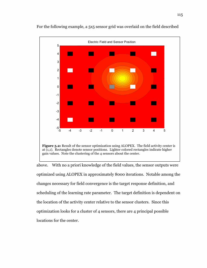
115
For the following example, a 5x5 sensor grid was overlaid on the field described
above. With no a priori knowledge of the field values, the sensor outputs were
optimized using ALOPEX in approximately 8000 iterations. Notable among the
changes necessary for field convergence is the target response definition, and
scheduling of the learning rate parameter. The target definition is dependent on
the location of the activity center relative to the sensor clusters. Since this
optimization looks for a cluster of 4 sensors, there are 4 principal possible
locations for the center.
Electric Field and Sensor Position
-5 -4 -3 -2 -1 0 1 2 3 4 5-5
-4
-3
-2
-1
0
1
2
3
4
5
Figure 5.2: Result of the sensor optimization using ALOPEX. The field activity center is at (1,1). Rectangles denote sensor positions. Lighter colored rectangles indicate higher gain values. Note the clustering of the 4 sensors about the center.

116
If the center is equidistant from the four corners of the square the sensors
define, then the target value is 4/3. This can be found by evaluating the field
intensities under each sensor. Using the same logic, if the center is located
equidistant between 2 sensors (i.e. on the side of the square), then the target
remains 4/3. If the center is directly under a sensor, then the result is slightly
different: (4/3 + 1/9). Given these target possibilities, 1.3 was used as the
training target in all simulations.
The value of the learning rate parameter was initially defined using the gain
scheduling mentioned above. However, under this condition the system did not
converge. By using smooth transitions between values for the learning rate
0 5000 100000
0.5
1
1.5
MSV
Epochs
0 5000 100000
0.5
1
1.5
MSV
Epochs
0 5000 100000
0.5
1
1.5
MSV
Epochs
0 5000 100000
0.5
1
1.5
MSV
Epochs
0 5000 100000
0.5
1
1.5MSV
Epochs
0 5000 100000
0.5
1
1.5
MSV
Epochs
0 5000 100000
0.5
1
1.5
MSV
Epochs
0 5000 100000
0.5
1
1.5
MSV
Epochs
0 5000 100000
0.5
1
1.5
MSV
Epochs
0 5000 100000
0.5
1
1.5
MSV
Epochs
0 5000 100000
0.5
1
1.5
MSV
Epochs
0 5000 100000
0.5
1
1.5
MSV
Epochs
0 5000 100000
0.5
1
1.5
MSV
Epochs
0 5000 100000
0.5
1
1.5
MSV
Epochs
0 5000 100000
0.5
1
1.5
MSV
Epochs
0 5000 100000
0.5
1
1.5
MSV
Epochs
Figure 5.3: Response versus iteration plots for each of the candidate clusters. Note the maximum value generated by the plot corresponding to the position of the center.

117
parameter, and having it increase linearly after training iteration 1000, the
system did converge. It is assumed that this high learning rate parameter was
necessary to have sufficient changes late in the training time course to support
convergence. The equation governing this parameter is:
(5.12)
An additional constraint must be mentioned. The range of the weights must be
restricted to [0,1] for the correlation logic discussed above to operate properly.
Under these conditions, the target of 1.3 and the constraint on the weights,
training occurred in 8000 iterations, as mentioned above, with the other center
locations training in markedly shorter times.
Locating the center of activity on the “edge” of a square is direction independent.
This is to say that the training setup and performance are not different for centers
located between two sensors horizonally versus one located between two sensors
vertically. This is most likely due to the orthogonal rotation invariance of the
template field, since the field is same if rotated multiples of 90 degrees about the
template center.
≥+
−
−
<
−
=−
−
1000,511000
100020
1000,15
)(
500
1000
10
kek
ke
kk
k
γ

118
Optimizing for this scenario, the two sensor edge case, showed markedly shorter
training time, as mentioned above. Training was achieved in roughly 7100
iterations, or about 10% less than the above case. Since these two sensors nearest
the activity center see a large field value, the response function changes more
rapidly. Also, this scenario has two possible optimization solutions, the left and
right squares formed by the sensor locations, as opposed to the single possible
solution above.
The training course versus iterations was similar to the previous result. As
before, the catastrophe effect can be seen late in training by noting the sharp drop
in response just before the target is met. This artifact is due in part to the high
Electric Field and Sensor Position
-5 -4 -3 -2 -1 0 1 2 3 4 5-5
-4
-3
-2
-1
0
1
2
3
4
5
Figure 5.4: Field optimization result for a center located equidistant from two sensors. As above, rectangles denote sensor locations and the whiter the sensor color, the higher the gain.

119
optimization target. In an effort to optimize to the target this sharp change
occurs, but ALOPEX compensates due to the change in sign of the response
function change, and returns to the previous training levels.
Continuing with the final case in the sensor to field relationship, simulations
were conducted placing the activity center directly under the sensor at position
(0,0). In this alignment, there are four potential solutions, one for each square
that has a corner at the sensor located above the sensor. This leads to four
“corner” solutions: upper left, lower left, upper right, and lower right. Each of
0 2000 4000 6000 80000
0.5
1
1.5
MSV
Epochs
0 2000 4000 6000 80000
0.5
1
1.5
MSV
Epochs
0 2000 4000 6000 80000
0.5
1
1.5
MSV
Epochs
0 2000 4000 6000 80000
0.5
1
1.5
MSV
Epochs
0 2000 4000 6000 80000
0.5
1
1.5
MSV
Epochs
0 2000 4000 6000 80000
0.5
1
1.5
MSV
Epochs
0 2000 4000 6000 80000
0.5
1
1.5
MSV
Epochs
0 2000 4000 6000 80000
0.5
1
1.5
MSV
Epochs
0 2000 4000 6000 80000
0.5
1
1.5
MSV
Epochs
0 2000 4000 6000 80000
0.5
1
1.5
MSV
Epochs
0 2000 4000 6000 80000
0.5
1
1.5
MSV
Epochs
0 2000 4000 6000 80000
0.5
1
1.5
MSV
Epochs
0 2000 4000 6000 80000
0.5
1
1.5
MSV
Epochs
0 2000 4000 6000 80000
0.5
1
1.5
MSV
Epochs
0 2000 4000 6000 80000
0.5
1
1.5MSV
Epochs
0 2000 4000 6000 80000
0.5
1
1.5
MSV
Epochs
Figure 5.5: Training vs. Iterations for the 2 sensor vertical edge case in Fig. 5.3. Note the two solutions at lower right that both approach the threshold value. These represent the two sensor “squares” that share the edge on which the activity center lies. Note the catastrophe effect artifact in the (3,3) plot just before training completed.

120
Electric Field and Sensor Position
-5 -4 -3 -2 -1 0 1 2 3 4 5-5
-4
-3
-2
-1
0
1
2
3
4
5
0 200 400 600 8000
0.5
1
1.5
MSV
Epochs
0 200 400 600 8000
0.5
1
1.5
MSV
Epochs
0 200 400 600 8000
0.5
1
1.5
MSV
Epochs
0 200 400 600 8000
0.5
1
1.5
MSV
Epochs
0 200 400 600 8000
0.5
1
1.5
MSV
Epochs
0 200 400 600 8000
0.5
1
1.5
MSV
Epochs
0 200 400 600 8000
0.5
1
1.5
MSV
Epochs
0 200 400 600 8000
0.5
1
1.5
MSV
Epochs
0 200 400 600 8000
0.5
1
1.5
MSV
Epochs
0 200 400 600 8000.5
1
1.5
MSV
Epochs
0 200 400 600 8000
0.5
1
1.5
MSV
Epochs
0 200 400 600 8000
0.5
1
1.5
MSV
Epochs
0 200 400 600 8000
0.5
1
1.5
MSV
Epochs
0 200 400 600 8000
0.5
1
1.5
MSV
Epochs
0 200 400 600 8000
0.5
1
1.5
MSV
Epochs
0 200 400 600 8000
0.5
1
1.5
MSV
Epochs
Figure 5.6: Field optimization for single sensor directly over the sensor. Note the cluster of four candidate solutions at the center and some catastrophe effect artifacts in the training.

121
these sensor clusters has equal exposure to the field activity, and thus an equal
chance at being the chosen solution. As expected, this scenario trained much
faster, in about 680 iterations, with the four “corner” solutions showing
comparable performace. The sensor over the activity sensor always has high
gain, with the other three sensors in the square having varying gains.
5.5 Computational Efficiency and Application
These simulations were conducted in MATLAB both for programming
convenience and for display of the data. Since MATLAB is designed for matrix
mathematics and since the optimization approach is matrix based, it was the
logical choice. Though optimization here took several minutes, the lags were
mostly due to MATLAB’s background and display overhead. Efficiently coded on
an embedded processor, this optimization would occur in near real time, on the
order of seconds.
The intent of this optimization is to compensate for changes in the system. For
example, if the location of the sensors changed, this algorithm would compensate
by selecting the proper set of sensors. Also, if the user’s activity, for example
EMG intensities, changed due to use of the device or muscle atrophy, such
changes would again be compensated for by this optimization.

122
Chapter 6: Conclusions and Future Work
The above chapters present a study of the development of robotic manipulators
for prosthetic hand applications, from design, to assembly, control,
programming, and simulation. Previous work, namely DeLaurentis (2004) dealt
with the design and manufacture of such mechanisms. In addition to mechanical
exploration via the development of the aforementioned novel right angle
transmission, herein, the focus has been on the control algorithms and hardware
to be used with the associated systems.
Further, the combination of virtual solid modeling environments with the
capabilities of fused deposition modeling (FDM) allowed for the integration of
the transmission output shaft at the proximal end of the several digit links.
The Microchip controllers combined to provide a bridge from USB to I2C,
allowing the control of the system via PC. Internally, the programs on the
controllers handle proportional feedback control of the joints. This combined
with motor drivers shows the viability of low level control board production in a
space comparable to that available in a potential prosthetic device.
While similar to previous approaches using similar hardware (Carrozza, et al.
2008), the hardware herein takes advantage of bus architectures for
expandability and standardization. Rather than using RS-232 serial
communication, for which one port is needed for each target processor, the use of

123
the I2C bus allows for “tacking on” of additional control units. Also, the use of
USB standardizes the interface with computers. Rather than needing specific
hardware, like the National Instruments cards used by Carrozza et al, any USB
capable computer with proper software can be used to control this architecture.
Further, it should be noted, that the use of surface mounted components, the
elimination of redundant power supply circuitry used for modularity in testing,
and development of 4-layer PCB layouts for the circuits leads to the potential of
embedding this controller in a space comparable to that of a human palm in vivo.
Control of the device has been demonstrated to be non-linear, since torque due to
gravity varies with the sine of the angle from horizontal. The use of model
reference adaptive control (MRAC) shows that the system parameters need not
be known to control the system presented above. Further, incorporation of
computational intelligence methods, namely artificial neural networks (ANN),
provides a more desirable response when incorporated with MRAC (ANN-
MRAC). In both of the above cases, MRAC and ANN-MRAC, following the
initialization of the system, the simulated controller was able to make the system
track the model presented to the controller without knowledge of the system
parameters and compensating for the non-linearity in gravitational torque.
ANN-MRAC carries an additional benefit. While most control solutions deal with
achieving a target, the performance of a biomimetic system, like that of an
artificial hand prosthesis, depends not only on reaching the target, but also the
trajectory taken to reach it. Consider for example, a slow grasp and a fast grasp.

124
The use of MRAC reduces the communication overhead between the processors
since a complete time course for the joint need not be sent. These data may be
several hundred values for even short lived motions. Rather, the parameters for
the reference model, which can be as few as 2 numbers, are all the information
needed to define a trajectory to present to the controller.
The combination of the above three aspects: mechanical design and fabrication,
electronic hardware design and fabrication, and control system design and
simulation, gives a framework for the development of an integrated system for
use as a prosthetic hand. Rapid mechanical prototyping, herein through FDM,
provides a mechanism for custom fabrication of mechanical parts of nearly
arbitrary shape and dimension. The rapid production of complex circuitry,
including surface mount technology is possible with the use of PCB technology.
The simulation of controls shows the feasibility of intelligent control schemes for
use in an artificial hand. All these, combined with the low cost and modularity of
the manipulator developed here lends to the use of this design and architecture in
a full hand scenario.
In addition, the sensor network optimization, while considered herein as a
general case, is directly applicable to detection of volition by a prosthesis user.
The ability to neglect the exact sensor positions in favor of higher dimensional
data makes application of sensors for such detection less dependent on the
individuals using or applying the system. An added benefit is the rejection of
human error, as the interface is designed adaptively based on the user’s

125
performance. Since the attention paid to each sensor is determined through
optimization, the evolution of the user’s inputs (think, for example, of changes in
writing habits) could be compensated for through the adaptation of the network.
This leads to a more robust interface, and reduced costs from the ease of
application.
6.1 Conclusion
Compared to the existing technologies, this work offers several new approaches
to problems facing prosthetic technology. A key factor in design of such a device
is the availability. Reduction of cost necessarily increases the pool of patients
able to afford and use a prosthesis. While the Smoovy actuators used in
Cyberhand are more compact than the DC motor and transmission developed
here, the presented alternative costs less than $100 per joint, depending on the
fabrication method for the digit links. Also, the electronic hardware developed
for control of those joints is very low cost, an estimated $50 per local controller,
and $20 per supervisory controller.
Sophistication in the control algorithms would improve the efficacy of a
prosthesis. Variation of the trajectory to cause different closing rates has not
previously been considered. However, control of the path of each digit may
provide more life-like motions and make the device a more effective replacement
for lost function. The MRAC methods described here allow for specification of
the trajectory with minimal communication overhead.

126
Maintenance is also a factor in the life cycle of a prosthesis. The less the system
needs to be adjusted, the more uninterrupted use would be and thus the user
would realize more benefit from the device. Using adaptive methods to
compensate for changes in sensor locations and signal characteristics over time
allows the controller to update itself. Since this does not require human
intervention, adding such intelligence improves the performance of the device
automatically. Also, by training the system to the user, less patient learning time
is necessary, and thus the patient realizes the benefit of the replaced function
sooner.
6.2 Future Work
6.2.1 Extension to Multi-Joint Control
As noted in the above commentary on adaptive control of the digit, the torque
due to gravity is a significant non-linear term in the mathematical model of the
digit. Using the above model for a single joint, extension of the control
simulations to a multi-joint configuration is possible. Deriving the relationship
between the several joint angles would allow for complete modeling of the digit,
taking into account gravity and changes in rotational inertia as the configuration
of the digit changes. This full model provides a test platform for higher level
computational intelligence methods, for coordination and perhaps more optimal
control given the additional information.

127
6.2.2 Construction and Testing of a Complete Artificial Hand
Perhaps the most obvious future work derived from this project is the replication
of the manipulator presented here for use in an artificial hand. Some
modification would be necessary for the development of an artificial thumb, but
the above designs would be usable for the other 4 digits, with some modification
in length.
A key consideration in such a design would be the control of it. As mentioned
above in 3.1, the changes of the system parameters with changes in joint angles
would have to be evaluated. The simulations of MRAC and ANN-MRAC
presented in the work may prove useful in the design of the embedded controllers
necessary for this application. Also, additional processing power may be
necessary to handle the several tasks and processes within a period suitable for
control of the several digits and joints therein.
6.2.3 Extension of the Electronic Hardware
Although the above mentioned circuitry was developed specifically to control the
modular finger actuator, we foresee use of this architecture in several extensible
scenarios. Before modification to the architecture is made, improvements to the
circuitry itself would be desirable. Most apparent among the potential changes
would be the use of surface mount technology, and possibly 4 layer (instead of 2
layer) boards in order to shrink the control circuitry further. However, a major
problem to overcome is the assembly of such a circuit without a reflow oven.

128
Since so little of the high level or master processor’s input/output functionality is
used, additional sensing or interface options present themselves. As alluded to
earlier, with the remote reset and remote interrupt options on the low level
processors, the master processor could remotely reset a processor having
difficulty, or interrupt a processor if an error occurred or another change needed
to be made.
Also, we mentioned above a USB host, without specifying it. This USB host could
be a personal computer, as we used in testing, or an embedded processor.
Several ARMs and xScale processors with USB host functionality are available to
handle embedded high level processing. Also, some of these come with Bluetooth
capability. This wireless avenue presents many potential applications, including
wireless monitoring and higher level networking.

129
References
[1] Abboudi, R., Class, C.A., Newby, N.A., Flint, J.A., & Craelius, W. (1999) A Biomimetic Controller for a Multifinger Prosthesis. IEEE Transactions on Rehabilitation Engineering. 7:121-129.
[2] *Ackermann, J. (1985) Sampled Data Control Systems: Analysis and
Synthesis, Robust System Design. Springer-Verlag, Berlin. [3] Al-Olimat, K.S., Girman, G., Kurtz, E.J., and Swarthout, H.J. (2003)
Transfer Function Evaluation in MRAC for Synchronous Machine Speed. Proceedings of the 2003 IEEE Conference on Control Applications: 920-924.
[4] Andersen, D.W. (2003) Praise the Lord and Pass the Penicillin: Memoir of a
Combat Medic in the Pacific in World War II. McFarland, London. [5] Bertoluzzo, M., Buja, G.S., and Todesco, F. (1994) Neural Network Adaptive
Control of a DC Drive. 20th International Conference on Inducstrial Electronics, Control, and Instrumentation, pp. 1232-1236.
[6] Bia, A. (2000) A Study of Possible Improvements to the Alopex Training
Algorithm. Proceedings of the 6th Brazilian Symposium on Neural Networks. pp. 125-130.
[7] Burdea, G. C. (1996) Force and Touch Feedback for Virtual Reality; John
Wiley and Sons, New York. [8] Boyne, W.J. (2003) Operation Iraqi Freedom; Forge, New York. [9] Bundhoo, V., Haslam, E., Birch, B., and Park, E.J. (2008) A Shape Memory
Alloy Based Tendon Driven Actuation System for Biomimetic Artificial Fingers, Part I: Design and Evaluation. Robotica First View article.
[10] Carrozza, M.C., Cappiello, G., Micera, S., Edin, B.B., Beccai, L., & Cipriani, C.
(2006) Design of a Cybernetic Hand for Perception and Action. Biological Cybernetics. 95:629-644.
[11] Carrozza, M.C., Persichetti, A., Laschi, C., Vecchi, F., Vacalebri, P.,
Tamburrelli, V., Lazzarini, R., & Dario, P. (2005) A Novel Wearable Foot Interface for Controlling Robotic Hands. 2005 IEEE/RSJ International Conference on Intelligent Robots and Systems. pp. 2010-2015.
[12] Cheung, J.Y.M., Cheng, K.W.E., and Kamal, A.S. (1996) Motor Speed
Control by Using a Fuzzy Logic Model Reference Adaptive Controller. Power Electronics and Variable Speed Drives, September 23-25, 1996.

130
[13] Cipriani, C., Zaccone, F., Micera, S., & Carrozza, M.C. (2008) On the Shared Control of an EMG-Controlled Prosthetic Hand: Analysis of User-Prosthesis Interaction. IEEE Transactions on Robotics. 24:170-184.
[14] Cipriani, C., Zaccone, F., Stellin, G., Beccai, L., Cappiello, G., Carrozza, M.C.,
& Dario, P. (2006) Closed-loop Controller for a Bio-inspired Multi-fingered Underactuated Prosthesis. Proceedings of the 2006 IEEE International Conf on Robotics and Automation. pp. 2111-2116.
[15] Cranny, A., Cotton, D.P.J., Chappell, P.H., Beeby, S.P., & White, N.M. (2005)
Thick Film force and slip sensors for a prosthetic hand. Sensors and Actuators A: Physical 123-124:pp. 162-171.
[16] Crnosija, P., Ban, Z., & Krishnan, R. (2002) Application of Model Reference
Adaptive Control to PM Brushless DC Motor Drives. Proceedings of the 2002 IEEE International Symposium on Industrial Electronics. pp. 689-694.
[17] Codfelter, M.D. (1992) Warfare and Armed Conflicts: A Statistical Reference
to Casualty and Other Figures 1618-1991; McFarland & Co., Jefferson, NC. [18] Cooley, T. & Micheli-Tzanakou, E. (1998) Classification of Mammograms
Using a Modular Neural Network. Journal of Intelligent Systems. 8:1-53. [19] Cowdrey, A.E. (1994) Fighting for Life: American Military Medicine in
World War II; The Free Press, New York. [20] Craelius, W (2002) The Bionic Man: Restoring Mobility. Science 295:1018-
1021 [21] Curcie, D.J., Flint, J.A., Craelius, W. (2001) Biomimetic Finger Control by
Filtering of Distributed Forelimb Pressures. IEEE Transactions on Neural Systems and Rehabiliation Engineering. 9:69-75.
[22] DeLaurentis, K.J. (2004) “Development of New Methodologies for the
Fabrication and Actuation of Robotic Systems;” Doctoral Dissertation, Rutgers University, May 2004.
[23] Dempsey, G.L., Alig, J.S., & Redfield, D.E. (1996) Using Analog Neural
Networks for Control Sensor Linearization. Proceedings of the 38th Midwest Symposium on Circuits and Systems. pp. 73-76.
[24] Doshi, R., Yeh, C., & LeBlanc, M. (1998) The design and development of a
gloveless endoskeletal prosthetic hand. Journal of Rehabilitation Research and Development. 35:388-395.
[25] Ehsani, M.S. (2007) Adaptive Control of Servo Motor by MRAC Method.
2007 Vehicle Power and Propulsion Conference. pp. 78-83.

131
[26] Erickson, J.E., DeLaurentis, K.J., and Bouzit, M. (2007a) A Novel Single
Digit Manipulator for Prosthetic Hand Applications. 2007 IEEE Systems and Information Engineering Design Symposium, Charlottesville, VA, April 2007.
[27] Erickson, J.E., DeLaurentis, K.J., and Bouzit, M. (2007b) A Novel Method of
Transmission of Rotational Motion Between Non-Parallel Axes. 2007 ASME Applied Mechanics and Materials Conference, Austin, TX, June 2007.
[28] Flint J.A., Phillips, S.L., & Craelius, W. (2003) Myo-Kinetic Interface For A
Virtual Limb. 2nd International Workshop on Virtual Rehabilitation. pp. 113-118.
[29] Franklin, G.F., Powell, D.J., and Emami-Naeini, A. (2002) Feedback Control
of Dynamic Systems; Prentice Hall, New York. [30] Frayman, Y. and Wang, L. (1999) Direct MRAC with Dynamically
Constructed Neural Controllers. 1999 International Joint Conference on Neural Networks. IJCNN99: 2236-2240.
[31] Ge, S.S., Lee, T.H., & Harris, C.J. (1998) Adaptive Neural Network Control of
Robotic Manipulators. World Scientific Publishing, Singapore. [32] Goodwin, G.C., Ramadge, P.J., Caines, P.E. (1979) Discrete Time
Multivariable Adaptive Control. 18th IEEE Conference on Decision and Control including the Symposium on Adaptive Processes. pp. 335-340.
[33] Greenberg, M.D. (1998) Advanced Engineering Mathematics, 2nd Edition.
Prentice Hall, Upper Saddle River, NJ. [34] Hartcup, Guy. (2000) The Effect of Science on the Second World War; St.
Martin’s Press, New York. [35] Harth, E. and Pandya, A.S. (1988) “Dynamics of ALOPEX Process:
Application to Optimization Problems.” in Biomathematics and related Computational Problems, Ricciardi, L.M., Ed. Kluwer, Boston, pp. 459-471.
[36] Harth, E. and Tzanakou, E. (1974) ALOPEX: A Stochastic Method for
Determining Visual Receptive Fields. Vision Research 14:1475-1482. [37] Hayakawa, T., Haddad, W.M., Hovakimyan, N. (2008) Neural Network
Adaptive Control for a Class of Nonlinear Uncertain Dynamical Systems with Asymptotic Stability Guarantees. IEEE Transactions on Neural Networks. 19:80-89.
132
[38] Haykin, S. Chen, Z., and Becker, S. (2004) Stochastic Correlative Learning Algorithms. IEEE Transactions on Signal Processing. 52:2200-2209.
[39] Heim, W. (2005) Microprocessor Technology for Powered Upper Extremity
Prosthetic Control Systems. Robotica. 23:275-276. [40] Hu, J., Hwang, X., and Chen, J. (1992) Neural Networks Adaptive Control.
Proceedings of the 1992 IEEE International Symposium on Industrial Electronics.
[41] Hudgins, B. and Parker, P. (1993) A New Strategy for Multifunction
Myoelectric Control. IEEE Transactions on Biomedical Engineering. 40:82-94.
[42] Jury, E.I. (1964) Theory and Application of the z-Transform Method. John
Wiley & Sons. New York. [43] Kargov, A., Asfour, T., Pylatiuk, C., Oberle, H., Klosek, H., Schulz, S.,
Regenstein, K., & Bretthauer, G. (2005) Development of an Antropomorphic Hand for a Mobile Assistive Robot. 9th International Conference on Rehabilitation Robotics. ICRR:182-186.
[44] Karr, C.L. (1999) Practical Applications of Computational Intelligence for
Adaptive Control. CRC Press. New York. [45] Kyberd, P.J., Evans, M., and te Winkel, S. (1998) An Intelligent
Anthropomorphic Hand, with Automatic Grasp. Robotica 16:531-536. [46] Kyberd, P.J., Light, C.M., Chappell, P.H., Nightingale, J.M., Whatley, D., &
Evans, M. (2001) The design of anthropomorphic prosthetic hands: a study of the Southampton Hand. Robotica 19:593-600.
[47] †Landau, Y.D. (1979) Adaptive Control: The Model Reference Approach.
Marcel Dekker. New York. [48] Li, S-J., Zhang, X-J., Qian, F. (2005) Soft Sensing Modeling via Artificial
Neural Network Based on PSO-ALOPEX. Proceedings of the 4th Int’l Conf on Machine Learning and Cybernetics. Guangzhou.
[49] Light, C.M. and Chappel, P.H. (2000) Development of a lightweight and
adaptable multiple-axis hand prosthesis. Medical Engineering and Physics 22:679-684.
[50] Light, C.M., Chappell, P.H., Hudgins, B., & Engelhart, K. (2002) Intelligent
multifunction myoelectric control of hand prosthesis. Journal of Medical Engineering Technology. 26:139-146.

133
[51] Lynch, K.F., Drew, J.G., Tripp, R.S., Roll, C.R. (2005) Lessons from Operation Iraqi Freedom; RAND, Arlington, VA.
[52] Medrano-Marques, N.J. & Martin-del-Brio, B. (2001) Sensor Linearization
with Neural Networks. IEEE Transactions on Industrial Electronics. 48:1288-1290.
[53] Meng, Q.H.M. and Lu, W.S. (1993) A Neural Network Adaptive Control
Scheme for Robot Manipulators. 1993 IEEE Conference of the Pacific Rim: 606-609.
[54] Micera, S., Carrozza, M., Beccai, L., Vecchi, F., Dario, P. (2006) Hybrid
Bionic Systems for the Replacement of Hand Function. Proceedings of the IEEE. 94:1752-1762.
[55] Micheli-Tzanakou, E. (2000) Supervised and Unsupervised Pattern
Recognition: Feature Extraction and Computational Intelligence; CRC Press, Boca Raton, FL.
[56] Microchip, “PIC18F2450/2550/4450/4550 Data Sheet”, Retrived from
microchip.com July 10, 2008. [57] Microchip, “PIC18F2331/2431/4331/4431 Data Sheet”, Retrieved from
microchip.com July 10, 2008. [58] Miller, D.E. (2003) A New Approach to Model Reference Adaptive Control.
IEEE Transactions on Automatic Control. 48:743-757. [59] Mitchell, P.D. (2004) Medicine in the Crusades: Warfare, Wounds, and the
Medieval Surgeon; Cambridge University Press, New York. [60] Ohka, M. and Kondo, S. (2008) Stochastic Resonance Aided Tactile Sensing.
Robotica First View Article. [61] Phillips, C.L. and Nagle, H.T. (1994) Digital Control System Design and
Analysis; Prentice Hall, New York. [62] Phillips, S.L. and Craelius, W. (2005) Residual Kinetic Imaging: a Versatile
Interface for Prosthetic Control. Robotica 23:277-282. [63] Pons, J.L., Ceres, R., Rocon, E., Reynaerts, D., Saro, B., Levin, S., & Van
Moorleghem, W. (2005a) Objectives and technological approach to the development of the multifunctional MANUS upper limb prosthesis. Robotica 23:301-310.

134
[64] Pons, J.L., Ceres, R., Rocon, E., Levin, S., Markovitz, I., Saro, B., Reynaerts, D., & Van Moorleghem, W. (2005b) Virtual reality training and EMG control of the MANUS hand prosthesis. Robotica 23:311-317.
[65] Pons, J.L., Ceres, R., and Pfeiffer, , F. (1999) Multifingered dextrous robotics
hand design and control: a review. Robotica 17:661-674. [66] Porat, B. (1997) A Course in Digital Signal Processing. John Wiley and Sons,
New York. [67] Pylatiuk, C., Mournier, S., Kargov, A., Schulz, S., & Bretthauer, G. (2004)
Progress in the Development of a Multifunctional Hand Prosthesis. Proceedings of the 26th Annual International Conference of the IEEE Engineering in Medicine and Biology Society. pp. 4260-4263.
[68] Rowcliffe, P. and Feng, J. (2008) Training Spiking Neuronal Networks with
Applications in Engineering Tasks. IEEE Transactions on Neural Networks 19:1626-1640.
[69] Schulz, S., Pylatiuk, C., & Bretthauer, G. (2001) A New Ultralight
Anthropomorphic Hand. Proceedings of the 2001 IEEE International Conference on Robotics and Automation: 2437-2441
[70] Schulz, S., Pylatiuk, C., Reischl, M., Martin, J., Mikut, R., & Bretthauer, G.
(2005) A hydraulically driven multifunctional prosthetic hand. Robotica 23:293-299.
[71] Scott, R.W. and Collins, D.J. (1990) Neural Network Adaptive Controllers.
The 1990 International Joint Conference on Neural Networks. [72] Shadow Robot Company. (2005) “Shadow Dexterous Hand C3 Technical
Specification,” draft received December 2005. [73] Shadow Robot Company. (2004) “Developments in Dexterous Hands for
Advanced Robotic Applications,” copy provided by the company December 2005.
[74] Shadow Robot Company. (2003) Design of a Dexterous Hand for Advanced
CLAWAR Applications. Proceedings of the 6th Int’l Conf on Climbing and Walking Robots (CLAWAR): Catania, Italy; September 17-19, 2003. (Provided by Shadow Robot Company, December 2005)
[75] Solarbotics, Ltd. (2003) “The ‘Secret’ L293D Motor Driver.” Solarbotics,
Ltd. Calgary, Alberta. [76] ST Microelectronics (2003) “L293D/L293DD Datasheet.” Retrieved from
digikey.com August 23, 2008.

135
[77] Stoten, D.P. (1990) Model Reference Adaptive Control of Manipulators.
John Wiley and Sons. New York. [78] Sunwoo, M., Cheok, K.C., and Huang, N.J. (1991) Model Reference Adaptive
Control for Vehicle Active Suspension Systems. IEEE Transactions on Industrial Electronics. 38:217-222.
[79] Tao, G. (1997) Robustness of MRAC Schemes. Proceedings of the American
Control Conference: 744-745. [80] Tao, G. & Ioannou, P.A. (1993) Model Reference Adaptive Control of Plants
with Unknown Relative Degree. IEEE Transactions on Automatic Control. 38:976-982.
[81] Tzanakou, E., & Harth, E. (1973) Determination of Visual Receptive Fields
by Stochastic Methods. Biophysical Society Abstracts. 13:42a. [82] United States Department of Defense (2008) “Casualty Update.” Retrieved
from http://www.defenselink.mil/news/casualty.pdf, December 8, 2008. [83] Unnikrishnan, K.P. & Venugopal, K.P. (1992) Learning in Connectionist
Networks Using the ALOPEX Algorithm. 1992 International Joint Conference on Neural Networks. pp. 926-931.
[84] Venugopal, K.P., Pandya, A.S., and Sudhakar, R. (1992) ALOPEX Algorithm
for Adaptive Control of Dynamical Systems. The 1992 International Joint Conference on Neural Networks, pp. 875-880.
[85] Watson, R.K. (2008) “2008 FRC-RC Example Code and Utilities.” Available
at www.kevin.org/frc/. Retrieved July 10, 2008. [86] Wetterhahn, R. (2001) The Last Battle: The Mayaguez Incident and the End
of the Vietnam War; Carroll and Graf, New York. [87] Wikipedia: The Free Encyclopedia “United States Casualties of War.”
Accessed August 12, 2008: http://en.wikipedia.org/wiki/United_States_casualties_of_war.
[88] Wininger, M., Kim, N-H., & Craelius, W. (2008) Pressure Signature of
Forearm as Predictor of Grip Force. Journal of Rehabilitation Research and Development. 45:883-892.
[89] Winter, S.H. (2006) A Haptic Force Feedback Glove Using
Magnetorheologic Fluid. Unpublished Master’s Thesis. Rutgers University.

136
[90] Winter, S.H. & Bouzit, M. (2007) Use of Magnetorheological Fluid in a Force Feedback Glove. IEEE Transactions on Neural Systems and Rehabilitation Engineering. 15:2-8.
[91] Yamanaka, O., Yoshizawa, N., Ohmori, H. and Sano, A. (1997) Adaptive
Control and Stability Analysis of Nonlinear Systems Using Neural Networks. 1997 International Conference on Neural Networks.
Bibliographical Notes: * This work by Jürgen Ackermann is an English translation of the German Language work Abtastregelung by the same author in 1972. † Landau, Y.D. sometimes cites as Landau, I.D. in the literature.

137
Curriculum Vita
Jeffrey Edward Erickson August 2000 - May 2004 University of Virginia Bachelor of Science, Electrical Engineering Minor, Biomedical Engineering April 2007 – May 2009 ANADIGICS, Inc. Test Instrumentation & Data Acquisition Engineer August 2004 – May 2009 Rutgers, The State University of New Jersey University of Medicine and Dentistry of New Jersey Graduate Program in Biomedical Engineering Doctor of Philosophy Publications: Erickson, J.E. & Bouzit, M. (2006) "Development of a high degree of freedom hand prosthesis." 2006 Annual Meeting of the BMES Erickson, J.E., DeLaurentis, K.J. & Bouzit, M. (2007) "A Novel Single Digit Manipulator for Prosthetic Hand Applications," 2007 IEEE Systems and Information Engineering Design Symposium, Charlottesville, VA. Dicken, G., Butler, N., Kutch, M.E., & Erickson, J.E. (2007) "Application of Intelligent Control to the 2007 FIRST Robotics Competition," 2007 IEEE Systems and Information Engineering Design Symposium, Charlottesville, VA. Erickson, J.E., DeLaurentis, K.J. & Bouzit, M. (2007) "A Novel Method for Transmission of Rotational Motion Between Non-Parallel Axes," 2007 ASME Applied Mechanics and Materials Conference, Austin, TX. Dicken, G., Frank, R., Wasser, B., Kutch, M.E., Tompkins, W., & Erickson, J.E. (2008) "Data Collection for Performance Analysis and Fault Detection in the 2008 FIRST Robotics Competition," 2008 IEEE Systems and Information Engineering Design Symposium, Charlottesville, VA. Papers submitted for review: Erickson, J.E. & Micheli-Tzanakou, E. “Electronic Hardware for Embedded Control of Multiactuator Robotic Systems” IEEE Transactions on Circuits and Systems. Erickson, J.E. & Micheli-Tzanakou, E. “Adaptive Optimization of High Dimensionality Sensor Arrays using ALOPEX ” IEEE Transactions on Neural Systems and Rehabilitation Engineering.