integration of hydraulic and water quality modelling in ... · integration of hydraulic and water...
TRANSCRIPT

Integration of Hydraulic and Water Quality Modellingin Distribution Networks: EPANET-PMX
Alemtsehay G. Seyoum1,3 & Tiku T. Tanyimboh1,2
Received: 1 August 2016 /Accepted: 19 June 2017 /Published online: 25 July 2017# The Author(s) 2017. This article is an open access publication
Abstract Simulation models for water distribution networks are used routinely for manypurposes. Some examples are planning, design, monitoring and control. However, underconditions of low pressure, the conventional models that employ demand-driven analysisoften provide misleading results. On the other hand, almost all the models that employpressure-driven analysis do not perform dynamic and/or water quality simulations seamlessly.Typically, they exclude key elements such as pumps, control devices and tanks. EPANET-PDXis a pressure-driven extension of the EPANET 2 simulation model that preserved the capabil-ities of EPANET 2 including water quality modelling. However, it cannot simulate multiplechemical substances at once. The single-species approach to water quality modelling isinefficient and somewhat unrealistic. The reason is that different chemical substances mayco-exist in water distribution networks. This article proposes a fully integrated networkanalysis model (EPANET-PMX) (pressure-dependent multi-species extension) that addressesthese weaknesses. The model performs both steady state and dynamic simulations. It isapplicable to any network with various combinations of chemical reactions and reactionkinetics. Examples that demonstrate its effectiveness are included.
Keywords Water distribution network .Water qualitymodelling . Disinfection and disinfectionby-products . Drinkingwater standards . Pressure-driven analysis . Reaction kinetics
Water Resour Manage (2017) 31:4485–4503DOI 10.1007/s11269-017-1760-0
Electronic supplementary material The online version of this article (doi:10.1007/s11269-017-1760-0)contains supplementary material, which is available to authorized users.
* Tiku T. [email protected]
Alemtsehay G. [email protected]
1 Department of Civil and Environmental Engineering, University of Strathclyde, Glasgow, 75Montrose Street, James Weir Building, Glasgow G1 1XJ, UK
2 School of Civil and Environmental Engineering, University of the Witwatersrand, Private Bag 3,Wits, Johannesburg 2050, South Africa
3 SWS Consultancy, Addis Ababa, Ethiopia

1 Introduction
Water quality models simulate the spatial and temporal variations of the concentrations ofchemical substances in a water distribution network by combining the reaction kinetics withthe underlying hydraulics of the distribution network. The models have many applications e.g.designing sampling and monitoring programmes and optimizing the disinfection process. Theycan improve the calibration of hydraulic simulation models and assist in predicting thedeterioration of water quality (Clark 2015).
EPANET-MSX (multi-species extension) (Shang et al. 2008a, b) is a model that analyses waterquality in distribution networks using the dynamic link library of EPANET2, a hydraulic simulationmodel (Rossman 2000). It analyses multiple chemical substances simultaneously (Sun et al. 1999),accounts for any differences in the quality ofwater from different sources and provides a frameworkthat permits the simulation of any chemical or biological constituent. Multi-species water qualitymodels have many applications that address real-world water quality problems that are generallycomplex. Examples include the reactions of chlorine in distribution networks, chloramine decayand predictions of the reactivity of water supplied from various points (Shang et al. 2008a).
Though undesirable, pressure deficiency can occur due to selective mains closure formaintenance and repair purposes, pipe bursts, pump breakdowns, power failures and largeunanticipated demands for fire fighting. Conventional demand-driven hydraulic models forwater distribution systems presume demands are fully satisfied even if a network is in apressure-deficient condition. This assumption is true only when the network operates undernormal pressure conditions. Additionally, low-pressure conditions can facilitate the entry ofpathogenic microorganisms through pathways such as cracks and leaks (Besner et al. 2011;Nygard et al. 2007; Hunter et al. 2005). Thus, it is essential to have an integrated model thatcan simulate both pressure deficiency and water quality realistically and seamlessly.
There have been many endeavours to develop realistic pressure-driven analysis methods formore than three decades, and the models have been utilised to address a range of issuesincluding reliability evaluation, parameter calibration, reliability-based design, placement ofisolation valves and leakage management (Gupta and Bhave 1996; Giustolisi et al. 2008;Tsakiris and Spiliotis 2014; Elhay et al. 2015). Recently, significantly improved solutions tosome benchmark optimization problems were achieved using pressure-driven analysis (Siewet al. 2014, 2016). However, the models have not been considered in water quality studiesconcerned with issues such as loss of disinfection residual and intrusion of contaminants underlow-pressure conditions (Rathi and Gupta 2015; Rathi et al. 2016).
The most efficient approach for pressure-driven analysis involves embedding the relation-ship between the flow and pressure at a demand node in the system of hydraulic equations(Ciaponi et al. 2015; Elhay et al. 2015; Kovalenko et al. 2014). The source code of EPANET 2was modified recently to provide a pressure-driven model called EPANET-PDX (pressure-dependent extension) (Seyoum and Tanyimboh 2016) by incorporating a logistic pressure-driven demand function (Tanyimboh and Templeman 2010) in the global gradient algorithm(Todini and Pilati 1988). It can simulate water quality under both normal and low-pressureconditions with only one chemical reaction at a time (Seyoum and Tanyimboh 2014).
However, the single-species approach is inefficient and somewhat unrealistic. Differentchemical substances may co-exist in water distribution systems, and it can be time consuming,for example, to simulate chlorine and various disinfection by-products one by one. Effectively,it can render evolutionary optimization algorithms that address water quality concerns imprac-ticable, as the number of simulations required would be excessively large.
4486 Seyoum A.G., Tanyimboh T.T.

EPANET-MSX is a water quality model based on EPANET 2. While EPANET-MSX cansimulate multiple species simultaneously, it is not suitable for operating conditions withinsufficient pressure. To address these gaps this paper proposes an integrated network analysismodel called EPANET-PMX (pressure-dependent multi-species extension) for steady state andextended-period analysis, single- and multi-species simulation plus demand- and pressure-driven analysis.
2 Water Quality Modelling
Water quality models often assume advective-reactive transport and consider the reactions inthe bulk flow and at the pipe wall; an approach that includes both advection and dispersion isavailable in Tzatchkov et al. (2002). The governing equations address the conservation of massand reaction kinetics and often assume complete and instantaneous mixing of water at thenodes and junctions, and storage facilities (Rossman and Boulos 1996; Rossman 2000; Clarkand Grayman 1998; Monteiro et al. 2015).
2.1 Constitutive Equations
The mass conservation equations for pipes, junctions and storage facilities may be summarisedbriefly as follows.
The mass conservation equation for pipes is (Rossman 2000)
∂Ci
∂t¼ −ui
∂Ci
∂xþ ri; ∀i ð1Þ
where Ci ≡C(i, x, t) is the reactant concentration in pipe i at location x at time t; ui ≡ u(i, t) is themean flow velocity in pipe i at time t; and ri ≡ r(Ci) is the rate of reaction. The equationassumes that longitudinal dispersion in the pipes is negligible.
The mass balance equation for node n is
∑j∈In
Qpj þ Qe
!C i; x; tð Þx¼0 ¼ ∑
j∈InQpjC j; x; tð Þx¼L j
� �þ QeCe; ∀i∈On; ∀n ð2Þ
where j and i respectively denote pipes with flow entering and leaving node n. In and On
respectively denote the sets of pipes with flow entering and leaving node n; Lj is the length ofpipe j; Qpj is the volume flow rate in pipe j; Qe and Ce are, respectively, the volume flow rateand reactant concentration for any external flow entering node n.
The mass balance equation for the sth storage facility (tank or service reservoir) is
∂ VsCsð Þ∂t
¼ ∑i∈I s
QpiC i; x; tð Þx¼Li
� �− ∑
j∈Os
QpjCs þ rs; ∀s ð3Þ
where Vs ≡ V(s,t) and Cs ≡ C(s,t) are, respectively, the volume in storage and reactantconcentration at time t; Is denotes the set of links supplying the storage facility with flow;Os denotes the set of links receiving flow from the facility; and rs ≡ r(Cs) is the rate of reaction.
Besides the reactions in the bulk flow, there may be reactions with biofilm, corrosion andother materials at the pipe walls. The reaction rate coefficient employed in EPANET 2 for thereactions at the pipe wall is (Rossman et al. 1994; Powell et al. 2004: 11-12)
Integration of Hydraulic and Water Quality Modelling 4487

kw* ¼ kwk f
R kw þ k f� � ð4Þ
where kw* is the wall reaction rate coefficient (1/time); kw is the wall reactivity coefficient(length/time); kf is the radial mass transfer coefficient (length/time); and R is the hydraulicradius. The value of kf depends on the molecular diffusivity of the reactive species and theturbulence of the flow.
Several kinetic models that are included in this article to demonstrate the effectiveness ofthe proposed framework for low-pressure conditions and multiple concurrent reactions aredescribed briefly here. Both the single-species (Eqs. 5 and 7) and two-species models withfast- and slow-reacting components (Eqs. 6, 8 and 9) (Helbling and Van Briesen 2009; Sohnet al. 2004; Amy et al. 1998) were considered for the disinfectant, chlorine, and predominantdisinfection by-products, trihalomethanes and haloacetic acids (Nieuwenhuijsen et al. 2000).
An inadequate chlorine residual in a distribution system may lead to bacterial regrowth(Clark and Haught 2005) and, consequently, water-borne diseases. Disinfection by-productsresult from the reactions of chlorine with natural organic compounds in water (Rodriguez et al.2004; Ghebremichael et al. 2008) and are associated with adverse health effects(Nieuwenhuijsen et al. 2000; Richardson et al. 2002; Nieuwenhuijsen 2005; Hebert et al. 2010).
The first-order (Rossman 2000) and parallel first-order (Helbling and Van Briesen 2009)kinetic models for chlorine decay are, respectively,
r CCð Þ≡ ∂CC
∂t¼ −kCC ð5Þ
CC tð Þ ¼ CC0 ρexp −k1tð Þ þ 1−ρð Þexp −k2tð Þ½ � ð6Þ
Recalling that the reactant concentrations vary with space and time as in Eqs. 1 to 3,CC ≡ CC(t) is the time-varying chlorine concentration at a demand node or junction; and CC0 isthe initial chlorine concentration at the node or junction in question. It is worth repeating thatthe water quality results relate to the fully developed operational cycle (typically 24 h). CC0 isthus the chlorine concentration at the node at time t = 0. k is the reaction rate constant, k1 and k2are the fast and slow chlorine decay coefficients, respectively, and ρ represents the fraction ofchlorine that reacts rapidly.
The first-order (Rossman 2000) and parallel first-order (Sohn et al. 2004) models fortrihalomethanes, and the parallel first-order model for haloacetic acids (Sohn et al. 2004)are, respectively,
r CTTHMð Þ≡ ∂CTTHM
∂t¼ k CL−CTTHMð Þ ð7Þ
CTTHM ¼ CC0 α 1−exp −k1tð Þð Þ þ β 1−exp −k2tð Þð Þ½ � ð8Þ
CHAA6 ¼ CC0 γ 1−exp −k1tð Þð Þ þ δ 1−exp −k2tð Þð Þ½ � ð9Þ
where CTTHM refers to the time-varying total concentration of trihalomethanes (TTHM) whileCL is the ultimate concentration (Rossman 2000). CHAA6 refers to the time-varying
4488 Seyoum A.G., Tanyimboh T.T.
concentration of haloacetic acids (HAA6) (i.e. six species), k is the reaction rate constant andCC0 is the initial chlorine concentration (as in Eq. 6). k1 and k2 are the fast and slow chlorinedecay coefficients, respectively, while α, β, γ and δ are empirical coefficients.
2.2 Brief Overview of the Computational Solution Methods
Eulerian and Lagrangian approaches are commonly used together with a hydraulic simulationmodel to solve the water quality equations computationally. The discrete volume method is anEulerian approach that Grayman et al. (1988) suggested. Each pipe is divided into equalsegments with completely mixed volumes. At each successive water quality time step, theconcentration within each segment is determined and transferred to the adjacent downstreamsegment. At nodes, the concentration is updated using a flow-weighted average of the inflows(Eq. 2). The resulting concentration is then transferred to all adjacent downstream segments.This process is repeated for each water quality time step until a different hydraulic conditionoccurs. When a new hydraulic condition occurs, the pipes are divided again and the processcontinues.
Liou and Kroon (1987) suggested a Lagrangian method that divides the pipes into segmentssimilarly. Unlike Eulerian methods, the water parcels in the pipes are tracked and, at each timestep, the length of the farthest upstream parcel in each pipe increases as water enters the pipewhile the farthest downstream parcel shortens as water leaves the pipe. The concentration atevery node is updated by a flow-weighted average of the inflows (Eq. 2). If the resulting nodalconcentration is significantly different from the concentration of an adjacent downstreamparcel, a new parcel is created at the upstream end of each link that receives flow from thenode. The process repeats for each water quality time step until a different hydraulic conditionoccurs and the procedure begins again.
Lagrangian methods can be either time- or event-driven. Time-driven methods update theconditions using a fixed time step whereas event-driven methods do so when the water qualityat the source changes or the front end of a parcel reaches a node. A comparison by Rossmanand Boulos (1996) indicated that the time-driven Lagrangian method was the most efficient.EPANET 2 and EPANET-MSX employ a time-driven Lagrangian approach (Rossman 2000;Shang et al. 2008b).
3 Integrated Network Analysis Model
It is worth recalling that EPANET-MSX is not a free-standing network analysis model in thesense that it has no hydraulic modelling capabilities. Instead, it uses the standard EPANETdynamic link library for the requisite hydraulic analyses the results of which are not accessible.Also, given the weaknesses of demand-driven analysis, a model for water quality analysis thatprovides realistic solutions for both normal and low pressure conditions is clearly necessary(Liserra et al. 2014).
An integrated model called EPANET-PMX (pressure-driven multi-species extension)was developed. It provides the full modelling functionality under both normal andpressure-deficient operating conditions in a way that is seamless. In other words,EPANET-PMX combines the modelling capabilities of EPANET 2, EPANET-MSX andEPANET-PDX. EPANET-PDX is an extension of EPANET 2. It includes a logisticpressure-driven nodal flow function (Tanyimboh and Templeman 2010) that was
Integration of Hydraulic and Water Quality Modelling 4489
incorporated in the system of equations in the global gradient algorithm (Todini andPilati 1988). The computational solution procedure developed (Seyoum 2015, Seyoumand Tanyimboh 2016) includes a line minimization algorithm (Dennis and Schnabel1996; Press et al. 2007) that improves convergence by optimizing the Newton steps inthe global gradient algorithm.
EPANET-PMX was developed by incorporating the pressure-driven analysis algorithmin the framework for the reaction kinetics in EPANET-MSX (Shang et al. 2008a, b). Theappendix includes an outline of the program. The convergence criteria were taken as amaximum change in the nodal heads of at most 0.001 ft. (3.048 × 10⁻⁴ m) and a maximumchange in the pipe flow rates of at most 0.001 cfs (2.832 × 10⁻⁵m3s−1) between successiveiterations (Seyoum and Tanyimboh 2016). The criterion used in EPANET 2 requires theratio of the sum of the absolute values of changes in the pipe flow rates to the sum of thepipe flow rates in successive iterations to be less than 10−3.
The data required to execute EPANET-PMX are as follows. (a) The standard EPANET 2input file that describes the properties of the pipes and nodes. (b) The standard EPANET-MSXinput file that specifies the water quality species and their reaction kinetics. (c) A data input filethat specifies the residual heads above which the nodal demands are satisfied in full, with thesame format as EPANET 2.
4 Results and Discussion
Selected results are shown here for water age, chlorine residual and disinfection by-products to illustrate and verify the capabilities of the proposed model. The verificationwas effected by comparing EPANET 2 and the MSX, PDX and PMX extensions.Various scenarios were considered for two networks. The first was a simple hypotheticalnetwork from the literature (Network 1 in Fig. 1) (Fujiwara and Ganesharajah 1993). Thesecond was a real network in the UK (Network 2 in Figure 2) (Seyoum and Tanyimboh2014).
Reasonably complete results could be presented here for Network 1, as it is quite small andthis network was selected in part for this reason. On the other hand, Network 2 is much largerand, aiming to reflect the entire network, representative results were included. The networkwas used previously to assess water quality simulation models and was selected in part for thisreason (Seyoum and Tanyimboh 2014).
All the simulations were carried out with an Intel Core 2 Duo personal computer (CPUof 3.2 GHz and RAM of 3.21 GB). In general, hydraulic and water quality models requireextensive calibration for operational use. However, the various investigations and proce-dures involved are outside the scope of this article. The effectiveness of the proposedintegrated model must be demonstrated first, followed by fieldwork and any additionalvalidation steps.
A constant chlorine concentration of 1 mg/L was assumed at each supply node, aiming toachieve a chlorine residual of at least 0.2 mg/L (WHO 2008) at the remote points in thenetworks (Seyoum and Tanyimboh 2014). A maximum TTHM concentration of 100 μg/L wasassumed in accordance with the Water Supply (Water Quality) Regulations (2010) in Englandand Wales, and was taken as the value of CL, i.e. the limiting concentration in Eq. 7. The waterquality time step was 5 min. Steady state conditions were assumed for Network 1 while thehydraulic time step for Network 2 was one hour.
4490 Seyoum A.G., Tanyimboh T.T.

Helbling and Van Briesen (2009) developed general-purpose empirical relationshipsbetween the initial concentration of chlorine and each parameter of the parallel first-orderchlorine decay model. Accordingly, the values adopted here were ρ = 0.87, k1 = 0.31/hand k2 = 0.02/h. Similarly, Sohn et al. (2004) developed empirical equations for thecoefficients of the parallel first-order kinetic models for trihalomethanes and haloaceticacids. Accordingly, the values adopted here were α = 16, β = 34.7, γ = 14.5 andδ = 10.3. Finally, both kb and k were taken as 1.0/day (Carrico and Singer 2009;Helbling and Van Briesen 2009; Seyoum and Tanyimboh 2014). The wall reactivitycoefficient kw requires calibration in practice and would require field data to bring abouta significant qualitative improvement in the results. This research is in progress; the pipewall reaction was not considered explicitly.
4.1 Network 1
Network 1 has one source node, six demand nodes and eight pipes of length 1000 m andHazen-Williams roughness coefficient of 140. The required residual head was 15 m for allthe demand nodes and the residual head below which there would be no flow was taken aszero. Steady state conditions were assumed. Source heads of 90 m, 65 m and 60 m wereconsidered with respective demand satisfaction ratio (DSR) values of 100%, 70% and56%. The demand satisfaction ratio is the available flow divided by the demand, i.e. thefraction of the demand that is satisfied.
Network 1 was analysed using both EPANET-MSX and EPANET-PMX. The results areshown in Figure 1. When pressure was sufficient, both EPANET-MSX and EPANET-PMXprovided essentially identical results. The expected trends of decreasing chlorine residualand increasing TTHM concentrations with the distance from the source are self-evident.The results confirmed also that the chlorine residual and TTHM concentrations at thesupply nodes were always 1.0 and zero, respectively, for all the pressure and DSRconditions. Both models analysed the fast- and slow-reacting components of chlorineand TTHM simultaneously in a single execution.
Furthermore, EPANET-PMX provided the concentrations of chlorine and TTHM thatreflected the actual pressure conditions. The deficiencies in pressure influenced the overallperformance of the system significantly. As the pressure decreased, the available flow atthe demand nodes decreased. The flow velocities decreased while travel times increased asa result. The simulated results reflected these effects. Reductions in the DSR increased thetravel times and TTHM concentrations but decreased the choline residual concentrations.It was revealed that the concentration of chlorine at node 6 would be less than theminimum requirement of 0.2 mg/l for a network DSR of 56%.
4.2 Network 2
Network 2 (Fig. 2) comprises 416 pipes, 380 demand nodes and four supply nodes (R1 toR4). Supply nodes R2 to R4 had a constant water level of 133 m. R1 is a variable-headsupply node whose average water level was 133 m. The pipe sizes range from 50 mm to500 mm and the total length of the pipes is 164 km. The demand categories consideredwere domestic demand, losses or unaccounted for water, and 10-h and 16-h commercialdemands for an operating cycle of 24 hours, as shown in Fig. 9 in the (online) supplemen-tary data.
Integration of Hydraulic and Water Quality Modelling 4491

Scenarios corresponding to supply node water levels ranging from 90 m to 133 mwere considered, in steps of 4 m, i.e. 12 cases for each model. The head below which the
(a) Network characteristics
(b) Chlorine and TTHM concentrations under normal pressure conditions. DSR was 100%.
0.65
0.75
0.85
0.95
1.05
0 1 2 3 4 5 6
Chlo
rine
(mg/
L)
Node IDEPANET- MSX EPANET- PMX
0
2
4
6
0 1 2 3 4 5 6
TTHM
(µg
/L)
Node IDEPANET-MSX EPANET-PMX
Legend:
The pipe diameters are shown in
millimetres in parentheses while
nodal elevations and demands are
shown in metres and litres per
second, respectively, in brackets.
[50, 47.1](500)
(250)
[50, 47.1]
(400)
(400)
(250)
(250)
(250)
[45, 77.8] [45, 47.1]
[55, 55.6] [55, 88.9]
(400)
(c) Chlorine and TTHM concentrations for low and normal pressure (EPANET-PMX)
0 0.2 0.4 0.6 0.8 1
0
1
2
3
4
5
6
Chlorine (mg/L)
Nod
e ID
DSR
56%
70%
100%
0 5 10 15 20 25
0
1
2
3
4
5
6
TTHM (µg/L)
Nod
e ID
DSR
56%
70%
100%
Fig. 1 Chlorine and TTHM concentrations in Network 1 under normal and low pressure conditions. DSR(demand satisfaction ratio) is available flow divided by demand
4492 Seyoum A.G., Tanyimboh T.T.

nodal flow would be zero was taken as the nodal elevation while the prescribed residualhead for full demand satisfaction was taken as 20 m. An operational period of 10 dayswas simulated, to avoid the inconsistent results at the beginning of the simulations. Water
(a) Network topology. R1 to R4 are supply nodes; the head at R1 is variable while R2-R4
are constant.
(b) Domestic demand (c) Unaccounted for water
(d) 10 hours commercial demand (e) 16 hours commercial demand
Fig. 2 Topology and demand categories of Network 2
Integration of Hydraulic and Water Quality Modelling 4493

age, chlorine residual, trihalomethanes and haloacetic acids were considered. The hy-draulic and water quality time steps were one hour and five minutes, respectively.Table 1 shows the accuracy of the results and CPU times of the various simulationmodels.
It is evident in Table 1 that EPANET 2 and EPANET-PDX were faster thanEPANET-MSX and EPANET-PMX when simulating one reactant in isolation. Itshould be clarified that EPANET-MSX has ‘command line’ and ‘toolkit’ variants whileEPANET-PMX is based on the toolkit. While the command line variant of EPANET-MSX isfaster, the toolkit provides more flexibility. For example, it enables programmers to customisethe software. EPANET-MSX (toolkit variant) and EPANET-PMX required averages of 856 and996 s, respectively, to analyse water age, chlorine residual, trihalomethanes and haloacetic acidsconcurrently. EPANET-MSX (command line variant) required 66 s. Besides the extra compu-tational demands of pressure-driven analysis, the differences in the simulation times are mainlyattributable to the toolkit.
4.2.1 Normal Pressure Conditions
The heads at all the supply nodes were fixed at 133 m to satisfy all the demands in full.Figure 3 and Table 1 show that EPANET-PMX and EPANET-MSX provided essentiallyidentical results except for several minor discrepancies in the water age. It is worthrepeating that EPANET-PDX and EPANET-PMX do not use the same convergencecriteria as EPANET 2 and EPANET-MSX (Seyoum and Tanyimboh 2016).
Table 1 Accuracy and computational properties for a network with 416 pipes (Network 2)
(a) Average CPU times (seconds)Simulations performed EPANET 2 EPANET PDX EPANET MSX EPANET PMXWater age 2 3 94 131Chlorine concentration 2 4 108 148TTHM concentration 6 9 112 167Water age and Chlorine*, TTHM*,
Chlorine+,TTHM+, HAA6+
concentrations at once
Not applicable Not applicable 856 996
†Total number of extended periodsimulations performed
36 36 48 48
*Based on the first-order models (Eqs. 5 and 7). + Based on the two-species models (Eqs. 6, 8 and 9). †Based on12 simulations per single- or multi-species analysis; in other words, each simulation was carried out 12 times.
(b) Deviations between EPANET PMX and MSX results for normal pressure conditionsDeviation criteria Water age
(hours)Chlorine
concentration(mg/L)
TTHMconcentration(μg/L)
HAA6concentration(μg/L)
Average deviation 0.051 0 0 0Maximum deviation 3.570 0 0 0Root mean square error 0.351 0 0 0(c) Linear correlation between the simulation results of EPANET 2, MSX, PDX and PMX (R2)
EPANET PMX Water age Chlorine TTHMEPANET 2 DSR = 100% 0.9999 0.9994 0.9997EPANET MSX DSR = 100% 0.9999 0.9999 0.9999EPANET PDX DSR = 100% 0.9999 0.9996 0.9999EPANET PDX DSR = 50% 0.9999 0.9996 0.9999DSR (demand satisfaction ratio) is the available flow divided by demand. Under conditions of normal pressure,
i.e. DSR = 100%, the correlation between EPANET MSX and PMX for HAA6 is R2 = 0.9999.
4494 Seyoum A.G., Tanyimboh T.T.

Consequently, the occasional minor difference may be considered reasonable. It wasrevealed that the residual chlorine concentration was less than 0.2 mg/L at a few demandnodes, based on the modelling parameters used (Figure 3b). This would be indicative ofa need for further investigations.
4.2.2 Low Pressure Conditions
Supply node heads of 112 m, 107 m, 102 m and 97 m that correspond to demand satisfactionratios of 90%, 75%, 50% and 30%, respectively, were investigated. Results for selected nodesare shown in Figs. 4 to 7. A reduction in the nodal flow rates due to low pressure leads to areduction in the pipe flow rates that causes the water age to increase. Consequently, theconcentration of chlorine decreases while the concentrations of the disinfection by-productsincrease.
The water age at node 6 was the lowest among the six selected nodes (Figure 4). Node6 has an advantageous relatively central location (Fig. 2) with respect to the supplynodes and nodes 1 to 5. By contrast, the water age at node 5 was relatively high; Figure 2shows that node 5 has a remote location relative to the four supply nodes. The chlorine,TTHM and HAA6 concentrations in Figs. 5, 6, 7 and 8 depend on the water age. In turn,the water age depends on the location within the network and the properties of the flowsupply paths in addition to pressure. For example, Figs. 5 and 8 show that the
(a) Water age (b) Chlorine residual
(c) TTHM (d) HAA6
0
10
20
30
40
50
0 100 200 300 400
Wate
r a
ge (
hrs)
Node ID
EPANET- PMX Difference from EPANET-MSX
0
0.2
0.4
0.6
0.8
1
0 100 200 300 400
Chlo
rin
e (
mg/L
)
Node ID
EPANET-PMX Difference from EPANET-MSX
0
10
20
30
40
0 100 200 300 400
Node ID
EPANET-PMX Difference from EPANET-MSX
0
5
10
15
20
25
0 100 200 300 400
Node ID
EPANET-PMX Difference from EPANET-MSX
Fig. 3 Water quality in Network 2 at 24:00 h under normal pressure conditions. TTHM and HAA6 denote totaltrihalomethanes and six species of haloacetic acids, respectively. This scenario revealed some nodes with chlorineresiduals of less than 0.2 mg/L.
Integration of Hydraulic and Water Quality Modelling 4495

concentration of chlorine at some nodes would be less than 0.2 mg/L for the abnormaloperating conditions shown.
The effects of closing the supply mains were investigated by closing all the supply nodesexcept for R2 the head at which was set at 133 m. Figure 8 depicts the EPANET-PMX results.This scenario illustrates simulations that might be performed for contingency and planningpurposes. In this scenario, node 3 is closest to the supply node R2 while nodes 1 and 4 arerelatively far. It can be seen that node 3 had the lowest water age and the highest residual
(a) Node 1 (b) Node 2
(c) Node 3 (d) Node 4
0
20
40
60
0 4 8 12 16 20 24
Wate
r a
ge (
hrs)
Time (hrs)
0
20
40
60
0 4 8 12 16 20 24
Wate
r a
ge (
hrs)
Time (hrs)
0
20
40
60
0 4 8 12 16 20 24
Wate
r a
ge (
hrs)
Time (hrs)
0
20
40
60
0 4 8 12 16 20 24
Wate
r a
ge (
hrs)
Time (hrs)
0
20
40
60
0 4 8 12 16 20 24
Wate
r a
ge (
hrs)
Time (hrs)
0
20
40
60
0 4 8 12 16 20 24
Wate
r a
ge (
hrs)
Time (hrs)
(e) Node 5 (f) Node 6
Fig. 4 Water age variations in Network 2 under low-pressure conditions. The demand satisfaction ratios (DSRs)were 30%, 50%, 75% and 90%
4496 Seyoum A.G., Tanyimboh T.T.
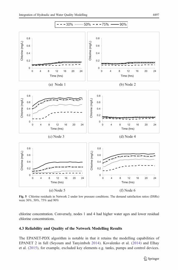
chlorine concentration. Conversely, nodes 1 and 4 had higher water ages and lower residualchlorine concentrations.
4.3 Reliability and Quality of the Network Modelling Results
The EPANET-PDX algorithm is notable in that it retains the modelling capabilities ofEPANET 2 in full (Seyoum and Tanyimboh 2014). Kovalenko et al. (2014) and Elhayet al. (2015), for example, excluded key elements e.g. tanks, pumps and control devices.
(a) Node 1 (b) Node 2
(c) Node 3 (d) Node 4
(e) Node 5
0
0.2
0.4
0.6
0.8
0 4 8 12 16 20 24
Chlo
rin
e (
mg/L
)
Time (hrs)
0
0.2
0.4
0.6
0.8
0 4 8 12 16 20 24
Chlo
rin
e (
mg/L
)
Time (hrs)
0
0.2
0.4
0.6
0.8
0 4 8 12 16 20 24
Chlo
rin
e (
mg/L
)
Time (hrs)
0
0.2
0.4
0.6
0.8
0 4 8 12 16 20 24
Chlo
rin
e (
mg/L
)
Time (hrs)
0
0.2
0.4
0.6
0.8
0 4 8 12 16 20 24
Chlo
rin
e (
mg/L
)
Time (hrs)
0
0.2
0.4
0.6
0.8
0 4 8 12 16 20 24
Chlo
rin
e (
mg/L
)
Time (hrs)
(f) Node 6
Fig. 5 Chlorine residuals in Network 2 under low pressure conditions. The demand satisfaction ratios (DSRs)were 30%, 50%, 75% and 90%
Integration of Hydraulic and Water Quality Modelling 4497

Control devices such as pressure regulating valves make the equations for water distribu-tion systems more difficult to solve (Kovalenko et al. 2014; Elhay et al. 2015). Theaccuracy and reliability of the EPANET-PDX results were verified previously (Seyoumand Tanyimboh 2014).
Herein, the accuracy of the EPANET-PMX results for Network 2 was verified withEPANET 2, EPANET-MSX and EPANET-PDX for normal pressure conditions. In addi-tion, EPANET-PDX was used for a low pressure condition with a demand satisfaction ratioof 50%. The comparisons were based on the first-order reaction models in Eqs. 5 and 7 to
(a) Node 1
(c) Node 3 (d) Node 4
(e) Node 5
0
8
16
24
32
40
0 4 8 12 16 20 24
Time (hrs)
0
8
16
24
32
40
0 4 8 12 16 20 24
Time (hrs)
0
8
16
24
32
40
0 4 8 12 16 20 24
Time (hrs)
0
8
16
24
32
40
0 4 8 12 16 20 24
Time (hrs)
0
8
16
24
32
40
0 4 8 12 16 20 24
Time (hrs)
0
8
16
24
32
40
0 4 8 12 16 20 24
Time (hrs)
(b) Node 2
(f) Node 6
Fig. 6 Concentrations of trihalomethanes in Network 2 under low pressure conditions. The demand satisfactionratios (DSRs) were 30%, 50%, 75% and 90%. TTHM denotes total trihalomethanes
4498 Seyoum A.G., Tanyimboh T.T.

ensure the results would be equitable. Consistently good results were achieved as shown inTable 1 and Fig. 3. Consistently good results were achieved for Network 1 also Figure 1.
5 Conclusions
Demand-driven models for water distribution networks provide unrealistic results underpressure-deficient conditions, which could lead to inappropriate investment and operationaldecisions. A pressure-driven, multi-species extension to the EPANET 2 simulation model was
(a) Node 1 (b) Node 2
(c) Node 3 (d) Node 4
(e) Node 5 (f) Node 6
0
5
10
15
20
25
0 4 8 12 16 20 24
Time (hrs)
10
15
20
25
0 4 8 12 16 20 24
Time (hrs)
0
5
10
15
20
25
0 4 8 12 16 20 24
Time (hrs)
0
5
10
15
20
25
0 4 8 12 16 20 24
Time (hrs)
0
5
10
15
20
25
0 4 8 12 16 20 24
Time (hrs)
0
5
10
15
20
25
0 4 8 12 16 20 24
Time (hrs)
Fig. 7 Concentrations of haloacetic acids in Network 2 under low pressure conditions. The demand satisfactionratios (DSRs) were 30%, 50%, 75% and 90%. HAA6 denotes six species of haloacetic acids
Integration of Hydraulic and Water Quality Modelling 4499

developed and demonstrated. The model can be applied to any network with differentcombinations of chemical reactions and reaction kinetics for all operating conditions fromzero flow to fully satisfactory flow and pressure. The accuracy of the results was checked andconsistently good results were achieved. Model calibration was not addressed in this article.More research is desirable, for example, to increase the speed of execution.
Acknowledgements This project was funded in part by the UK Engineering and Physical Sciences ResearchCouncil (EPSRC Grant Reference EP/G055564/1), the British Government (Overseas Research Students AwardsScheme) and the University of Strathclyde. The contribution of Richard Burd and Teddy Belrain of Veolia (nowAffinity) Water is gratefully acknowledged.
Compliance with Ethical Standards
Conflict of Interest There is no conflict of interest.
Appendix: Outline Description of the Software (EPANET-PMX)
On its own, EPANET-MSX has no hydraulic modelling capability; it performs hydraulicanalysis using EPANET’s dynamic library of functions. When used in this way, the results
(a) Water age (b) Chlorine
(c) TTHM (d) HAA6
0
4
8
12
16
0 4 8 12 16 20 24
Wa
ter a
ge
(h
rs)
Time (hrs)
0
0.2
0.4
0.6
0.8
1
0 4 8 12 16 20 24
Ch
lorin
e (
mg
/L)
Time (hrs)
0
5
10
15
20
25
30
0 4 8 12 16 20 24
Time (hrs)
0
5
10
15
20
25
30
0 4 8 12 16 20 24
Time (hrs)
Fig. 8 Water quality in Network 2 with only one supply node R2 available. R2 was available while R1, R3 andR4 were unavailable. TTHM and HAA6 denote total trihalomethanes and six species of haloacetic acids,respectively. These results from one extended period simulation illustrate the seamless integration of pressure-driven and multi-species network modelling
4500 Seyoum A.G., Tanyimboh T.T.
of the hydraulic analysis are not available to the end user. The proposed pressure-drivenextension was developed by modifying the source code of EPANET-MSX. It was achieved byembedding the EPANET-PDX pressure-driven hydraulic simulator in EPANET-MSX.
Furthermore, to create EPANET-PDX, the logistic pressure-driven nodal flow function(Tanyimboh and Templeman 2010) was embedded in the module for the global gradientalgorithm, Bnetsolve ()^, in EPANET 2. The pressure dependency upgrade included a lineminimization module, Blinesearch ()^, that performs the line search and backtracking topreserve the computational efficiency of the global gradient algorithm.
EPANET-MSX comprises a module, BMSXsolveH ()^, that performs extended periodhydraulic analysis. Also in EPANET-MSX is a module, BMSXinit ()^, that is called togetherwith another module, BMSXstep ()^, to initialize and perform the multi-species water qualityanalysis at each water quality time step.
Briefly, the data required to execute EPANET-PMX are as follows. (a) The EPANET 2input file that describes the properties of the links and nodes. (b) The EPANET-MSX input filethat specifies the water quality species and their reaction kinetics. (c) A data input file thatspecifies the residual heads (in feet) above which the nodal demands are satisfied in full,consistent with the EPANET 2 input file format. Additional details are available in theEPANET 2 and EPANET-MSX user manuals (Rossman 2000; Shang et al. 2008b).
Open Access This article is distributed under the terms of the Creative Commons Attribution 4.0 InternationalLicense (http://creativecommons.org/licenses/by/4.0/), which permits unrestricted use, distribution, and repro-duction in any medium, provided you give appropriate credit to the original author(s) and the source, provide alink to the Creative Commons license, and indicate if changes were made.
References
Amy G, Siddiqui M, Ozekin K, Zhu HW, Wang C (1998) Empirically based models for predicting chlorinationand ozonation by-products: haloacetic acids, chloral hydrate, and bromate. EPA Report CX 819579
Besner M-C, Prévost M, Regli S (2011) Assessing the public health risk of microbial intrusion events indistribution systems: conceptual model, available data, and challenges. Water Res 45(3):961–979
Carrico B, Singer PC (2009) Impact of booster chlorination on chlorine decay and THM production: simulatedanalysis. J Environ Eng 135(10):928–935
Ciaponi C, Franchioli L, Murari E, Papiri S (2015) Procedure for defining a pressure-outflow relationshipregarding indoor demands in pressure-driven analysis of water distribution networks. Water Resour Manag29:817–832. doi:10.1007/s11269-014-0845-2
Clark RM, Grayman WM (1998) Modelling water quality in drinking water distribution systems. AWWA,Denver
Clark RM, Haught RC (2005) Characterizing pipe wall demand: implications for water quality modelling. JWater Res Pl-ASCE 31(3):208–217
Clark RM (2015) The USEPA’s distribution system water quality modelling program: a historical perspective.Water Environ J 29(3):320–330
Dennis JE, Schnabel RB (1996) Numerical methods for unconstrained optimization and nonlinear equations.SIAM, Philadelphia
Elhay S, Piller O, Deuerlein J, Simpson A (2015) A robust, rapidly convergent method that solves the waterdistribution equations for pressure-dependent models. J Water Res Pl-ASCE. doi:10.1061/(ASCE)WR.1943-5452.0000578
Fujiwara O, Ganesharajah T (1993) Reliability assessment of water supply systems with storage and distributionnetworks. Water Resour Res 29(8):2917–2924
Ghebremichael K, Gebremeskel A, Trifunovic N et al (2008) Modelling disinfection by-products: couplinghydraulic and chemical models. Water Sci Technol Water Supply 8(3):289–295
Giustolisi O, Kapelan Z, Savic D (2008) Extended period simulation analysis considering valve shutdowns. JWater Res Pl-ASCE 134(6):527–537
Integration of Hydraulic and Water Quality Modelling 4501
Grayman WM, Clark RM, Males RM (1988) Modeling distribution-system water quality: dynamic approach. JWater Res Pl-ASCE 114(3):295–312
Gupta R, Bhave PR (1996) Comparison of methods for predicting deficient-network performance. J Water ResPl-ASCE 122(3):214–217
Helbling DE, Van Briesen JM (2009) Modelling residual chlorine response to a microbial contamination event indrinking water distribution systems. J Environ Eng 135(10):918–927
Hebert A, Forestier D, Lenes D et al (2010) Innovative method for prioritizing emerging disinfection by-products (DBPs) in drinking water on the basis of their potential impact on public health. Water Res44(10):3147–3165
Hunter PR, Chalmers RM, Hughes S, Syed Q (2005) Self-reported diarrhea in a control group: a strongassociation with reporting of low-pressure events in tap water. Clin Infect Dis 40(4):32–34
Kovalenko Y, Gorev NB, Kodzhespirova IF et al (2014) Convergence of a hydraulic solver with pressure-dependent demands. Water Resour Manag 28(4):1013–1031
Liou CP, Kroon JR (1987) Modeling the propagation of waterborne substances in distribution networks. J AmWater Works Assoc 79(11):54–58
Liserra T, Maglionico M, Ciriello V, Di Federico V (2014) Evaluation of reliability indicators for WDSs withdemand-driven and pressure-driven models. Water Resour Manag. doi:10.1007/s11269-014-0522-5
Monteiro L, Viegas RMC, Covas DIC, Menaia J (2015) Modelling chlorine residual decay as influenced bytemperature. Water Environ J 29(3):331–337
Nieuwenhuijsen MJ, Toledano MB et al (2000) Chlorination disinfection byproducts in water and theirassociation with adverse reproductive outcomes: a review. Occup Environ Med 57:73–85
Nieuwenhuijsen MJ (2005) Adverse reproductive health effects of exposure to chlorination disinfection by-products. Global NEST J 7(1):128–144
Nygard K, Wahl E, Krogh T et al (2007) Breaks and maintenance work in the water distribution systems andgastrointestinal illness: a cohort study. Int J Epidemiol 36(4):873–880
Powell J, Clement J, Brandt M et al. (2004) Predictive models for water quality in distribution systems. AWWAResearch Foundation
Press WH, Teukolsky SA, Vetterling WT, Flannery BP (2007) Numerical recipes: the art of scientific computing.Cambridge University Press
Rathi S, Gupta R (2015) Optimal sensor locations for contamination detection in pressure-deficient waterdistribution networks using genetic algorithm. Urban Water J. doi:10.1080/1573062X.2015.1080736
Rathi GR et al (2016) Risk based analysis for contamination event selection and optimal sensor placement forintermittent water distribution network security. Water Resour Manag. doi:10.1007/s11269-016-1309-7
Richardson SD, Simmons JE, Rice G (2002) Disinfection by-products: the next generation. Environ Sci Technol36(9):198A–205A
Rodriguez MJ, Serodes JB, Levallois P (2004) Behaviour of trihalomethanes and haloacetic acids in a drinkingwater distribution system. Water Res 38(20):4367–4382
Rossman LA, Boulos PF (1996) Numerical methods for modeling water quality in distribution systems: acomparison. J Water Res Pl-ASCE 122(2):137–146
Rossman LA, Clark RM, Grayman WM (1994) Modeling chlorine residuals in drinking-water distributionsystems. J Environ Eng 120(4):803–820
Rossman LA (2000) EPANET 2 users manual. national risk management research laboratory. US EnvironmentalProtection Agency, Cincinnati
Seyoum AG (2015) Head dependent modelling and optimization of water distribution systems. PhD thesis,University of Strathclyde, Glasgow
Seyoum AG, Tanyimboh TT (2014) Pressure dependent network water quality modelling. J Water Manage167(6):342–355. doi:10.1680/wama.12.00118
Seyoum AG, Tanyimboh TT (2016) Investigation into the pressure-driven extension of the EPANET hydraulicsimulation model for water distribution systems. Water Resour Manag 30(14):5351–5367. doi:10.1007/s11269-016-1492-6
Shang F, Uber JG, Rossman LA (2008a) Modelling reaction and transport of multiple species in waterdistribution systems. Environ Sci Technol 42(3):808–814
Shang F, Uber JG, Rossman LA (2008b) EPANET multi-species extension user’s manual. National RiskManagement Research Laboratory, US EPA, Cincinnati
Siew C, Tanyimboh TT, Seyoum AG (2014) Assessment of penalty-free multi-objective evolutionary optimiza-tion approach for the design and rehabilitation of water distribution systems. Water Resour Manag 28(2):373–389. doi:10.1007/s11269-013-0488-8
Siew C, Tanyimboh TT, Seyoum AG (2016) Penalty-free multi-objective evolutionary approach to optimizationof Anytown water distribution network. Water Resour Manag. doi:10.1007/s11269-016-1371-1
4502 Seyoum A.G., Tanyimboh T.T.

Sohn J, Amy G, Cho J, Lee Y, Yoon Y (2004) Disinfectant decay and disinfection by-products formation modeldevelopment: chlorination and ozonation by-products. Water Res 38(10):2461–2478
Sun Y, Petersen JN, Clement TP (1999) Analytical solutions for multiple species reactive transport in multipledimensions. J Contam Hydrol 35:429–440
Tanyimboh TT, Templeman AB (2010) Seamless pressure-deficient water distribution system model. J WaterManage 163(8):389–396
Todini E, Pilati S (1988) A gradient algorithm for the analysis of pipe networks. In: Coulbeck B, Chun-Hou O(eds) Computer applications in water supply: system analysis and simulation, vol 1. Research Studies Press,Taunton, pp 1–20
Tsakiris G, Spiliotis M (2014) A Newton-Raphson analysis of urban water systems based on nodal head-drivenoutflow. Eur J Environ Civil Eng 18(8):882–896
Tzatchkov VG, Aldama AA, Arreguin FI (2002) Advection-dispersion-reaction modeling in water distributionnetworks. J Water Res Pl-ASCE 128(5):334–342
Water Supply (Water Quality) Regulations (2010) No. 994 (W.99). Statutory Instrument. The Stationery Office,London
WHO (2008) Guidelines for drinking-water quality. WHO Press, Geneva
Integration of Hydraulic and Water Quality Modelling 4503