integration of remote sensing data and gis for prediction ... · integration of remote sensing data...
TRANSCRIPT
INTERNATIONAL JOURNAL OF GEOMATICS AND GEOSCIENCES Volume 1, No 4, 2011
© Copyright 2010 All rights reserved Integrated Publishing services Research article ISSN 0976 – 4380
847
Integration of Remote Sensing data and GIS for prediction of land cover map
Samereh Falahatkar 1 , Ali Reza Soffianian 1 , Sayed Jamaleddin Khajeddin 1 , Hamid Reza Ziaee 2 , Mozhgan Ahmadi Nadoushan 1
1 Natural resource faculty, Iafahan University of technology, Isfahan, Iran 2 Municipality of Isfahan, Iran
ABSTRACT
Satellite remote sensing and geographic information system (GIS) have been widely applied in identifying and analyzing land use and land cover change. In this study, aerial photos and MSS, TM and ETM + images of Isfahan and its environs were used to provide maps of land cover for 1955, 1972, 1990 and 2001. A hybrid method was used for image classification: a combination of supervised and unsupervised classification. Cellular automata filter facilities and Markov model were used together in a CAMarkov model for predicting land cover maps. To study the accuracy of the predicted maps and validation of the CAMarkov model, three methods were used: a calculating agreement and disagreement table, a chisquared goodnessoffit test and an error matrix. The results indicate that if land cover change processes are constant, the CA Markov model predicts land cover changes for the following years, for which agreement between predicted maps with actual map is less than 70% in this study area.
Key words: Change detection, CAMarkov model, Land cover
1. Introduction
Satellite remote sensing and geographic information system (GIS) have been widely applied in identifying and analyzing land use and land cover change (Jensen and Cowen, 1999; Hathout 2002). In recent years, these methods have progressed and have been used widely in management of natural resource and urban planning. Techniques based on multitemporal, multispectral, satellitesensor acquired data have demonstrated potential as a means to detect, identify, map and monitor ecosystem change, respective of the casual agents (Coppin et al., 2004). Land cover and land use change analyses and projection provide a tool to assess ecosystem changes and their environmental implication at various temporal and spatial scales (Lambin, 1997). There are a lot of methods for land cover change detection such as image rationing, image difference, change vector analysis, image regression, composite analysis and postclassification (Coppin et al., 2004). Detecting past changes and predicting these kinds of changes in the future play a key role in decision making and long term planning. Modeling is the main tool for studying land use and land cover change (Schneider and Pontius, 2001).
There are a lot of methods for land cover and land use change modeling that include mathematical equation based, system dynamic, statistical, expert system, evolutionary,
INTERNATIONAL JOURNAL OF GEOMATICS AND GEOSCIENCES Volume 1, No 4, 2011
© Copyright 2010 All rights reserved Integrated Publishing services Research article ISSN 0976 – 4380
848
cellular, and hybrid models. Cellular models (CM) include cellular automata (CA) and Markov models. In CA, each cell exists in one of a finite set of states, and future states depend on transition rules based on a local spatiotemporal neighborhood (Parker, 2002). Markov chain analysis is a convenient tool for modeling land cover and land use changes when changes and processes in the landscape are difficult to describe. Markov chains model is able to predict land use and land cover changes from one period to another and use this as the basis to project future changes (Estmen, 1995). Since first introduced by Ulam (1976) in 1948, cellular automata (CA) have been widely used to simulate nonlinear complex systems (Wolfram, 1984). CAbased models have a strong ability to represent nonlinear spatial and stochastic processes (Batty et al., 1997). Recently, cellular automata (CA) models have been applied in urban growth and land use change prediction (Yang et al., 2008).
To validate the simulations of land cover maps by a model, it should be calibrated with additional previous information to create a reference map for the simulated time (Pontius and Spencer, 2005). There are many techniques for validation; including the calculation of that one of them is budgets sources of agreement and disagreement between the prediction map and the reference map (Pontius et al., 2004). The percentage correct is budgeted by three components: agreement due to chance, agreement due to the predicted quantity of each land category, and agreement due to the predicted location of each land category. The percentage error is budgeted by two components: disagreement due to the predicted location of each land category and disagreement due to the predicted quantity of each land category. Therefore users can survey error sources and evaluate accuracy of model (Pontius and Spencer, 2005).
Detection of land cover change and prediction of future changes by CAMarkov models have been reported in several studies discussed in the following paragraphs.
Wijanarto (2006) investigates change detection and prediction of changes in land use in Serang, Indonesia by using ETM + (Enhanced Thematic Mapper) images from April 2000 and August 2001. ChengLiang Chang and JuiChin (2006) used SPOT data of Jiou Jiou Mountain from four different periods (March 1999, October 1999 and November 2002 & 2005) to study vegetation cover in 2006. Finally, they use Markov chain analysis and Cellular automata to predict temporal and spatial changes of vegetation cover. The paper concludes that CA Markov model is a more suitable method than others for the simulation of vegetation cover changes. Ayodeji Opeyemi (2006) detects land cover and land use changes of the Ilorin region in Kwara state by using GIS technology and remote sensing between 1972 and 2001 with the help of ETM + , TM and MSS data. After change detection in recent years he predicts land cover and land use changes for the next 14 years by using Markov and Cellular automata models.
The purpose of the current study is to prediction of land cover maps using CA Markov model in the study area and investigation of validation maps by comparing land cover maps produced by a hybrid method of image classification and prediction maps generated by the Markov model.
INTERNATIONAL JOURNAL OF GEOMATICS AND GEOSCIENCES Volume 1, No 4, 2011
© Copyright 2010 All rights reserved Integrated Publishing services Research article ISSN 0976 – 4380
849
2. Material and Method
2.1 Study area
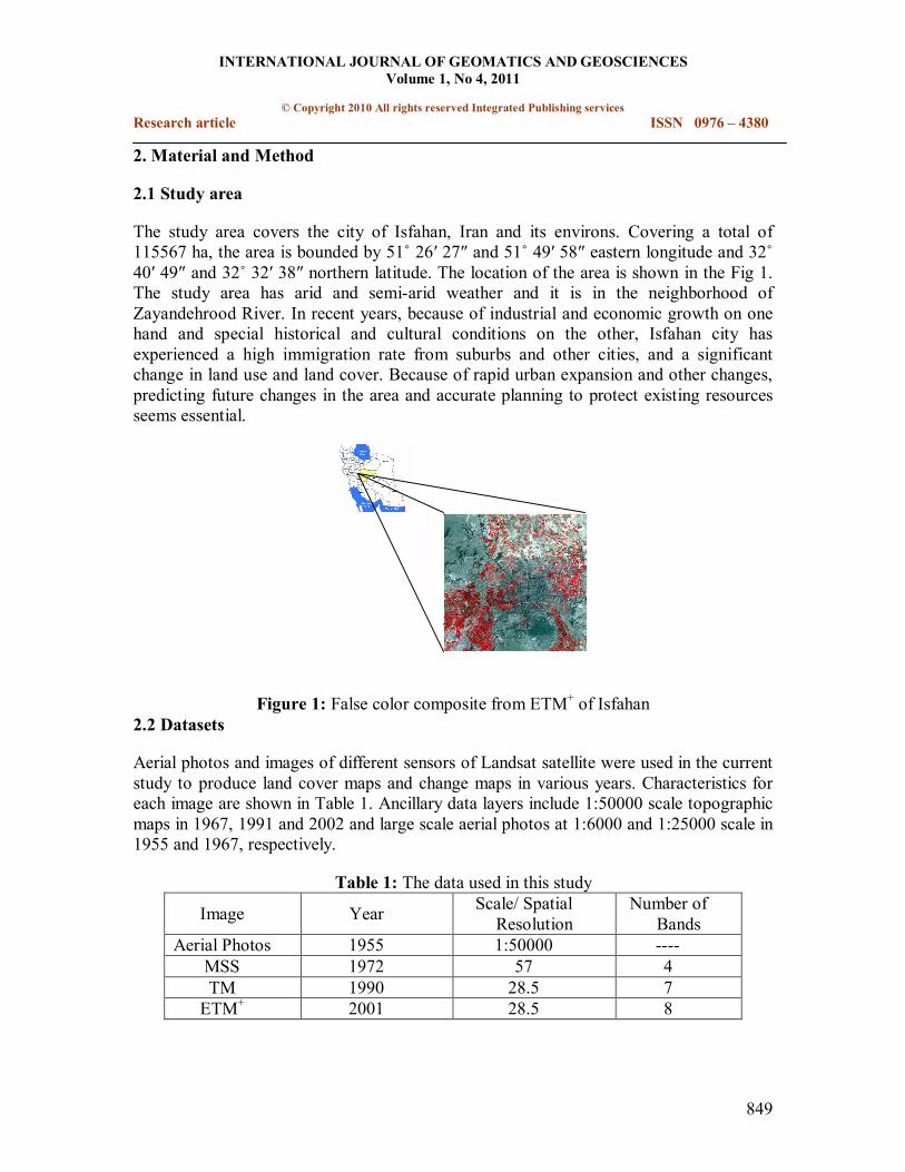
The study area covers the city of Isfahan, Iran and its environs. Covering a total of 115567 ha, the area is bounded by 51˚ 26′ 27″ and 51˚ 49′ 58″ eastern longitude and 32˚ 40′ 49″ and 32˚ 32′ 38″ northern latitude. The location of the area is shown in the Fig 1. The study area has arid and semiarid weather and it is in the neighborhood of Zayandehrood River. In recent years, because of industrial and economic growth on one hand and special historical and cultural conditions on the other, Isfahan city has experienced a high immigration rate from suburbs and other cities, and a significant change in land use and land cover. Because of rapid urban expansion and other changes, predicting future changes in the area and accurate planning to protect existing resources seems essential.
Figure 1: False color composite from ETM + of Isfahan 2.2 Datasets
Aerial photos and images of different sensors of Landsat satellite were used in the current study to produce land cover maps and change maps in various years. Characteristics for each image are shown in Table 1. Ancillary data layers include 1:50000 scale topographic maps in 1967, 1991 and 2002 and large scale aerial photos at 1:6000 and 1:25000 scale in 1955 and 1967, respectively.
Table 1: The data used in this study Number of
Bands Scale/ Spatial
Resolution Year Image
1:50000 1955 Aerial Photos 4 57 1972 MSS 7 28.5 1990 TM 8 28.5 2001 ETM +
INTERNATIONAL JOURNAL OF GEOMATICS AND GEOSCIENCES Volume 1, No 4, 2011
© Copyright 2010 All rights reserved Integrated Publishing services Research article ISSN 0976 – 4380
850
3. Methodology
3.1 Geometric correction
A firstorder polynomial method and nearest neighbor image resampling algorithm was applied for the geometric correction of aerial photos and satellite images. The RMS error of the aerial photos was in a range of 0.1 to 0.45 pixels. Then the georegistered aerial photos were mosaiced together. The RMSe of the transformation of MSS, TM and ETM + was 0.73, 0.68 and 0.6 pixels respectively. Rees et al. (2003) reported that RMSe in geometric correction of TM and ETM + images which were georeferenced to a topography map with 1:20000 scale were less than 1 pixel. Coppin et al. (2004) noted that an RMSe of less than 1 pixel for geometric correction of satellite images in a change detection process is acceptable.
3.2 Aerial photointerpretation
Aerial photointerpretation was carried out using standard photographic keys (tone, texture, pattern, shape and size). Interpretation of aerial photos was performed in mach line. We used a Stereomicroscope for accurate interpretation.
3.3 Image classification and accuracy assessment
To make the best false color composite, the Optimal Index Factor (OIF) was used. The OIF value is based on the amount of total variance and correlation between various band combinations. In this study, the supervised classification was performed using the maximum likelihood method and five land cover classes were identified including mountain, barren land, urban, green cover and river. Unsupervised classification was done with iterative self organizing data analysis (Isodata). NDVI and principal component analysis were used to separate the green cover and barren land respectively. The classification accuracy can be assessed by an error matrix. Many measurements have been proposed to improve the interpretation of the error matrix, among which the Kappa coefficient is one of the most popular measures. It is a discrete multivariate technique used in accuracy assessment (Congaltor, 1988). The reference data are collected from largescale aerial photos and topographic maps.
3.4 Change Detection
Change detection is the process of identifying differences in the state of an object or phenomenon by observing it at different times (Singh, 1989). It involves independently produced spectral classification results from each end of the time interval of interest, followed by a pixelbypixel or segmenttosegment comparison to detect changes in cover type. The principal advantage of post classification comparison lies in the fact that the two dates of imagery are separately classified; thereby minimizing the problem of radiometric calibration between dates (Copping, 2004).
INTERNATIONAL JOURNAL OF GEOMATICS AND GEOSCIENCES Volume 1, No 4, 2011
© Copyright 2010 All rights reserved Integrated Publishing services Research article ISSN 0976 – 4380
851
3.5 Land Cover Prediction
Markov chains have been widely used to model land use and land cover changes (Bell, 1974; Jahan, 1978; Robinson, 1978). Markov change models have several assumptions. One basic assumption is that land use and land cover is regarded as a stochastic process, and different categories are as the states of a chain (Weng, 2002); that is, it is only the most recent state (or link) that affects the transition to the next state: it is independent of prior history. The Markov chain can be expressed as
) ( ) ,...., , ( 1 1 1 1 1 1 0 0 − − − − = ⊥ = = = = = ⊥ = t t t t t t i X j X P i X i X i X j X P (Equation 1) (Fan et al., 2008).
This model is stochastic as opposed to dramatic, because model output, which is the distribution among states, is based on the probability of transition, Pij, between state i and j. Since the transitions are probabilities, it follows that:
∑=
= m
j ij P
1
1 i=1, 2, 3… m (Equation 2)
The transition probability is usually derived from a sample frequency of the transition occurring during some time interval (Baker, 1989). This is accomplished by developing a transition probability matrix of land use change from time one to time two, which will be the basis for projecting to a later time. The transition probabilities matrix records the probability that each land cover category will change to each other category. This matrix is the result of cross tabulation of two images adjusted by the proportional error (Estmen, 1995).
A CA model is a set of identical elements, called cells, each one of which is located in a regular and discrete space. Each cell can be associated with state from a finite set. The model evolves in discrete time steps, changing the state of each cell according to a transition rule homogeneously applied at every step. The new state of a certain cell depends on the previous states of a set of cells. Integrating a Markov chain model and a CA model provides a means of predicting temporal and spatial changes of land cover (Fan, 2008). In this study, we use a CAMarkov model for producing 1990 and 2001 maps and then compare them with the 1990 and 2001 maps produced by the hybrid method to study the capabilities of a CAMarkov model in predicting land cover changes.
3.6 Validation
As it is very important to validate model predictions, users need some powerful tools to measure the accuracy of predicted changes in land use models (Pontius, 2001). In this paper, in order to calculate the accuracy of prediction maps and validate the CAMarkov model three methods were used:
§ An agreement and disagreement table
INTERNATIONAL JOURNAL OF GEOMATICS AND GEOSCIENCES Volume 1, No 4, 2011
© Copyright 2010 All rights reserved Integrated Publishing services Research article ISSN 0976 – 4380
852
§ A chisquared goodnessoffit test § An error matrix
An agreement and disagreement table
To measure validation of predicted maps by the CAMarkov model, the VALIDATE function of Idrisi Kilimanjaro was used. VALIDATE provides a method to measure agreement between two categorical images, a "comparison" map and a "reference" map. The comparison map will usually be the result of a simulation or classification model whose validity is being assessed against a reference map that depicts reality (Estman, 1995).
A chisquare goodnessoffit test
This statistical test judges whether or not a particular distribution adequately describes a set of observations by making a comparison between the actual landcover area of observations and the expected landcover area of observations. The statistic is calculated from the relationship χ 2 =Σ(OiEi)/Ei
Where Oi is the observed and Ei the expected land cover area in 1990 and 2001. Hypotheses tested were:
H0: There are no significant differences between the observed areas (by means of hybrid classification) and the predicted areas (from CAMarkov model).
H1: The abovementioned differences are significant at α=0.05.
Error matrix
The error matrix and kappa coefficient are used to assess the accuracy of the classification procedure undertaken and may suggest ways to improve the classification.
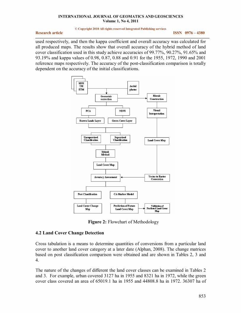
A method flow diagram of the process used is given in Figure 2.
4. Result and Discussion
4.1 Image Classification
The 1955 land cover map was produced by visual interpretation of aerial photos. The false color composites were generated from bands 3, 2 and 4 for MSS and 3, 4 and 7 for TM and ETM + by using the OIF index. Land cover classes in 1972, 1990 and 2001 were mapped from digital remotely sensed data though a hybrid process combining a supervised and unsupervised digital image classification. For accuracy assessment of the 1955 map, large scale aerial photos with a 1:6000 scale from the same year were used. For accuracy assessment of the 1972, 1990 and 2001 reference maps, aerial photos at a scale 1:25000 for 1967 and updated digital topography maps for 1991 and 2002 were
INTERNATIONAL JOURNAL OF GEOMATICS AND GEOSCIENCES Volume 1, No 4, 2011
© Copyright 2010 All rights reserved Integrated Publishing services Research article ISSN 0976 – 4380
853
used respectively, and then the kappa coefficient and overall accuracy was calculated for all produced maps. The results show that overall accuracy of the hybrid method of land cover classification used in this study achieve accuracies of 99.77%, 90.27%, 91.65% and 93.19% and kappa values of 0.98, 0.87, 0.88 and 0.91 for the 1955, 1972, 1990 and 2001 reference maps respectively. The accuracy of the postclassification comparison is totally dependent on the accuracy of the initial classifications.
Figure 2: Flowchart of Methodology
4.2 Land Cover Change Detection
Cross tabulation is a means to determine quantities of conversions from a particular land cover to another land cover category at a later date (Alphan, 2008). The change matrices based on post classification comparison were obtained and are shown in Tables 2, 3 and 4.
The nature of the changes of different the land cover classes can be examined in Tables 2 and 3. For example, urban covered 3127 ha in 1955 and 8321 ha in 1972, while the green cover class covered an area of 65019.1 ha in 1955 and 44808.8 ha in 1972. 36307 ha of

INTERNATIONAL JOURNAL OF GEOMATICS AND GEOSCIENCES Volume 1, No 4, 2011
© Copyright 2010 All rights reserved Integrated Publishing services Research article ISSN 0976 – 4380
854
the area which was green cover in 1955 was still green cover in 1972, but 5461.3 ha had been converted to urban use by 1972. As can be seen in Table 3, between 1972 and 1990, 7293.3 ha of green land was depredated and converted to urban use. During the same time period, 19453.3 ha of barren land were restored to green cover. 20% was changed to green cover. This occurred in the north of the study area and shows that aerial photos have a greater ability than MSS image data for separating urban area from other covers. Spectral mixing and spectral confusion between different land cover such as urban and barren land or urban and fallow agriculture fields are one of the most prevalent errors in image classification (Guindon et al. 2004).
The result of change detection from 1990 to 2001 shows that 7436.1 ha of green cover and 1991.1 ha of barren land were converted to urban use. At the same time the increase in green cover, from 1990 to 2001, was 2873.1 ha from urban and 4634.2 ha from barren land. During 19902001, 15% of the urban class was changed to green land. These changes may seem to be a classification error, but green land is among some of the urban areas for developing new housing. Streets and highways were generally classified as urban, but when urban tree canopies along the streets grow and expand, the associated pixels may be classified as green cover. We note that the changes from urban to green land occurred almost entirely near highways and streets: for example Chaharbagh bala and Charbagh paein streets. Yuan et al (2005) obtained the same results in their study. Converting river to urban and inverse change is most likely associated with omission and commission errors in the Landsat classification change map. Registration errors and edge effects can also cause apparent errors in the determination of change vs. nochange.
Table 2: Postclassification matrix of study area from 19551972 (ha)
Table 3: Postclassification matrix of study area from 19721990 (ha)
1955 Mountain Barren land Urban Green cover River Total
Mountain 10573.7 0 0 0 0 10573.7 Barren land 0 27818 441.3 23069.2 20.2 51199.6 Urban 0 664.3 2140.7 5461.3 46.7 8321 Green cover 0 7446.1 564.9 36307 474.5 44808.8 River 0 26.6 9 . 9 181.4 351.3 568
1972
Total 10573.7 35955.1 3127 65019.1 892.5 115567.7
1972 Mountain Barren land Urban Green cover River Total
Mountain 10573.7 0 0 0 0 10573.7
Barren land 0 27209.7 176 4560.5 9.8 33694.4 Urban 0 4499.7 6444.9 7239.3 128.4 18599.1 Green cover 0 19453.4 1692.6 32969 369.2 54529.2 River 0 28.5 7.3 39.8 60.5 136.2
1990
Total 10573.7 51199.6 8321 44808.8 568 115567.7
INTERNATIONAL JOURNAL OF GEOMATICS AND GEOSCIENCES Volume 1, No 4, 2011
© Copyright 2010 All rights reserved Integrated Publishing services Research article ISSN 0976 – 4380
855
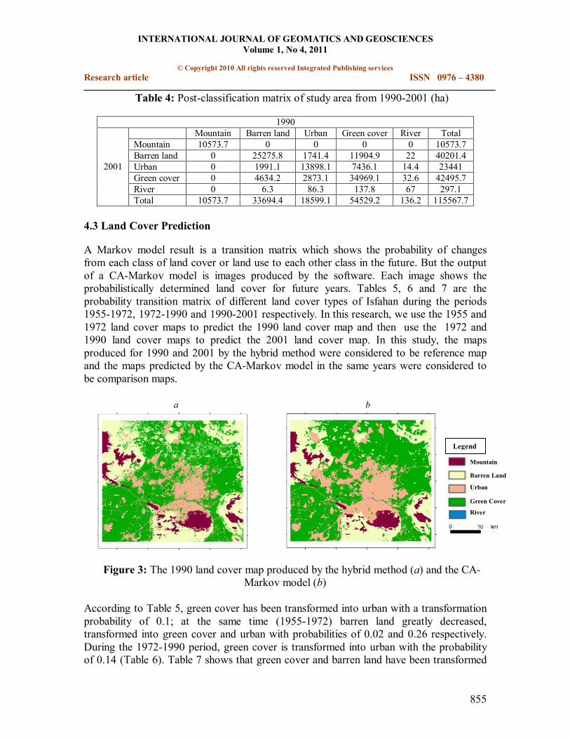
Table 4: Postclassification matrix of study area from 19902001 (ha)
4.3 Land Cover Prediction
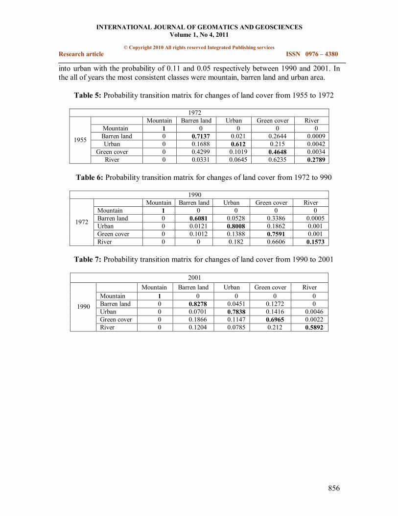
A Markov model result is a transition matrix which shows the probability of changes from each class of land cover or land use to each other class in the future. But the output of a CAMarkov model is images produced by the software. Each image shows the probabilistically determined land cover for future years. Tables 5, 6 and 7 are the probability transition matrix of different land cover types of Isfahan during the periods 19551972, 19721990 and 19902001 respectively. In this research, we use the 1955 and 1972 land cover maps to predict the 1990 land cover map and then use the 1972 and 1990 land cover maps to predict the 2001 land cover map. In this study, the maps produced for 1990 and 2001 by the hybrid method were considered to be reference map and the maps predicted by the CAMarkov model in the same years were considered to be comparison maps.
Figure 3: The 1990 land cover map produced by the hybrid method (a) and the CA Markov model (b)
According to Table 5, green cover has been transformed into urban with a transformation probability of 0.1; at the same time (19551972) barren land greatly decreased, transformed into green cover and urban with probabilities of 0.02 and 0.26 respectively. During the 19721990 period, green cover is transformed into urban with the probability of 0.14 (Table 6). Table 7 shows that green cover and barren land have been transformed
1990 Mountain Barren land Urban Green cover River Total
Mountain 10573.7 0 0 0 0 10573.7 Barren land 0 25275.8 1741.4 11904.9 22 40201.4 Urban 0 1991.1 13898.1 7436.1 14.4 23441 Green cover 0 4634.2 2873.1 34969.1 32.6 42495.7 River 0 6.3 86.3 137.8 67 297.1
2001
Total 10573.7 33694.4 18599.1 54529.2 136.2 115567.7
a
Barren Land
Mountain
Green Cover
Urban
River
Legend
b
INTERNATIONAL JOURNAL OF GEOMATICS AND GEOSCIENCES Volume 1, No 4, 2011
© Copyright 2010 All rights reserved Integrated Publishing services Research article ISSN 0976 – 4380
856
into urban with the probability of 0.11 and 0.05 respectively between 1990 and 2001. In the all of years the most consistent classes were mountain, barren land and urban area.
Table 5: Probability transition matrix for changes of land cover from 1955 to 1972
1972 Mountain Barren land Urban Green cover River
Mountain 1 0 0 0 0 Barren land 0 0.7137 0.021 0.2644 0.0009 Urban 0 0.1688 0.612 0.215 0.0042
Green cover 0 0.4299 0.1019 0.4648 0.0034
1955
River 0 0.0331 0.0645 0.6235 0.2789
Table 6: Probability transition matrix for changes of land cover from 1972 to 990
1990 Mountain Barren land Urban Green cover River
Mountain 1 0 0 0 0 Barren land 0 0.6081 0.0528 0.3386 0.0005 Urban 0 0.0121 0.8008 0.1862 0.001 Green cover 0 0.1012 0.1388 0.7591 0.001
1972
River 0 0 0.182 0.6606 0.1573
Table 7: Probability transition matrix for changes of land cover from 1990 to 2001
2001 Mountain Barren land Urban Green cover River
Mountain 1 0 0 0 0 Barren land 0 0.8278 0.0451 0.1272 0 Urban 0 0.0701 0.7838 0.1416 0.0046 Green cover 0 0.1866 0.1147 0.6965 0.0022
1990
River 0 0.1204 0.0785 0.212 0.5892

INTERNATIONAL JOURNAL OF GEOMATICS AND GEOSCIENCES Volume 1, No 4, 2011
© Copyright 2010 All rights reserved Integrated Publishing services Research article ISSN 0976 – 4380
857
Figure 4: The 2001 land cover map produced by the Hybrid method (a) and the CA Markov model (b)
4.4 Validation of Predictive Land Cover
Results of the agreement and disagreement components relating the prediction maps of 1990 and 2001 and reference maps according to the VALIDATE function were produced as shown in Tables 8 and 9. According to Table 8, the agreement of the 1990 maps is 0.6052 and the disagreement is 0.3948. These results for overall agreement of maps of the year 2001 is 0.6944 (Table 9) and overall disagreement for these two maps is 0.3056.
Table 8: A Table of agreement and disagreement of hybrid reference map and predictive map based on CAMarkov model (year 1990)
No[n] Medium[m] Perfect[p] Perfect[P(x)] P(n) 0.6366 P(m) 0.7764 P(p) 1
MediumGrid[M(x)] M(n) 0.4371 M(m) 0.6052 M(p) 0.6105 No[N(x)] N(n) 0.2 N(m) 0.3127 N(p) 0.3391
Table 9: Table of agreement and disagreement of hybrid and predictive maps based on CAMarkov model (year 2001)
No[n] Medium[m] Perfect[p] Perfect[P(x)] P(n) 0.6816 P(m) 0.872 P(p) 1
MediumGrid[M(x)] M(n) 0.4946 M(m) 0.6944 M(p) 0.6701 No[N(x)] N(n) 0.2 N(m) 0.3099 N(p) 0.3036
The second method of model validation is the chisquared goodnessfit test. This test is based on the number of pixels in each class or in the area of each class in the land cover map, and also compares the reference map and comparison map. The computed value of
Barren Land
Mountain
Green Cover
Urban
River
Legend
a b

INTERNATIONAL JOURNAL OF GEOMATICS AND GEOSCIENCES Volume 1, No 4, 2011
© Copyright 2010 All rights reserved Integrated Publishing services Research article ISSN 0976 – 4380
858
χ 2 is 25642 and 36915 for the 1990 and 2001 land cover maps which predicting by CA Markov respectively (with 4 degreeoffreedom at α=0.05) for above the accepted is threshold value of 0.711. The null hypothesis is rejected. Lopeza et al. (2001) used goodnessfit test to quantitatively assess the capabilities of Markov models in predicting different land use classes, and reported a value of 6677 for χ 2 , also showing that the land use areas predicted by Markov models have a statistically significant difference at α=0.05 when compared with land use areas of maps from aerial photo interpretation.
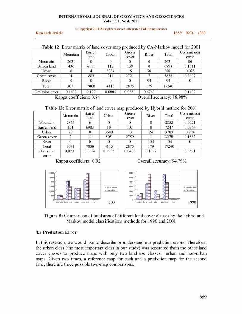
To calculate kappa coefficient and overall accuracy of all land cover maps, ground control points were used error matrix was calculated for land cover maps produced by both the hybrid method and the CAMarkov model. The kappa coefficient of prediction maps for the years 1990 and 2000 are 0.64 and 0.84 respectively, which are smaller than the hybrid method maps with kappa coefficients of 0.93 for the year 1990 and 0.92 for the year 2001 (Tables 10, 11, 12 and 13).
Table 10: Error matrix of land cover map produced by the CAMarkov method in 1990 Mountain Barren
land Urban Green cover River Total Commission
error Mountain 2587 238 53 0 0 2878 0.1011 Barren land 110 5988 1485 2441 7 10031 0.4036 Urban 0 0 1738 15 0 1753 0.0086
Green cover 0 105 501 4342 9 4957 0.1241 River 0 0 0 0 0 0 0 Total 2697 6331 3777 6798 16 19619
Omission error 0.0408 0.0542 0.5398 0.3613 1 0.253 Kappa coefficient: 0.64 Overall accuracy: 74.69%
Table 11: Error matrix of land cover map produced by the hybrid method for 1990 Mountain Barren
land Urban Green cover River Total Commission
error Mountain 2269 0 0 0 0 2269 0 Barren land 406 5945 1 12 0 6364 0.0658 Urban 0 0 3744 32 0 3776 0.0085
Green cover 22 386 32 6754 0 7194 0.0612 River 0 0 0 0 16 16 0 Total 2697 6331 3777 6798 16 19619
Omission error 0.1587 0.061 0.0087 0.0065 0 0.0454 Kappa coefficient: 0.93 Overall accuracy: 95.45%
INTERNATIONAL JOURNAL OF GEOMATICS AND GEOSCIENCES Volume 1, No 4, 2011
© Copyright 2010 All rights reserved Integrated Publishing services Research article ISSN 0976 – 4380
859
Table 12: Error matrix of land cover map produced by CAMarkov model for 2001 Mountain Barren
land Urban Green cover River Total Commission
error Mountain 2631 0 0 0 0 2631 00 Barren land 436 6111 112 139 0 6798 0.1011 Urban 0 4 3784 15 78 3881 0.025
Green cover 4 885 219 2721 7 3836 0.2907 River 0 0 0 0 94 94 0 Total 3071 7000 4115 2875 179 17240
Omission error 0.1433 0.127 0.0804 0.0536 0.4749 0.1102 Kappa coefficient: 0.84 Overall accuracy: 88.98%
Table 13: Error matrix of land cover map produced by Hybrid method for 2001 Mountain Barren
land Urban Green cover River Total Commission
error Mountain 2846 6 0 0 0 2852 0.0021 Barren land 151 6983 10 103 0 7247 0.0364 Urban 72 0 3600 13 24 3709 0.294
Green cover 2 11 505 2759 1 3278 0.1583 River 0 0 0 0 154 154 0 Total 3071 7000 4115 2875 179 17240
Omission error
0.0731 0.0024 0.1252 0.0403 0.1397 0.0521
Kappa coefficient: 0.92 Overall accuracy: 94.79%
Figure 5: Comparison of total area of different land cover classes by the hybrid and Markov model classifications methods for 1990 and 2001
4.5 Prediction Error
In this research, we would like to describe or understand our prediction errors. Therefore, the urban class (the most important class in our study) was separated from the other land cover classes to produce maps with only two land use classes: urban and nonurban maps. Given two times, a reference map for each and a prediction map for the second time, there are three possible twomap comparisons.
0
10000
20000
30000
40000
50000
60000
mountain Barren land urban green land river
Hybrid method
CA markov
0
10000
20000
30000
40000
50000
60000
mountain Barren land urban green land river
Hybrid Method
CA markov
1990 200
INTERNATIONAL JOURNAL OF GEOMATICS AND GEOSCIENCES Volume 1, No 4, 2011
© Copyright 2010 All rights reserved Integrated Publishing services Research article ISSN 0976 – 4380
860
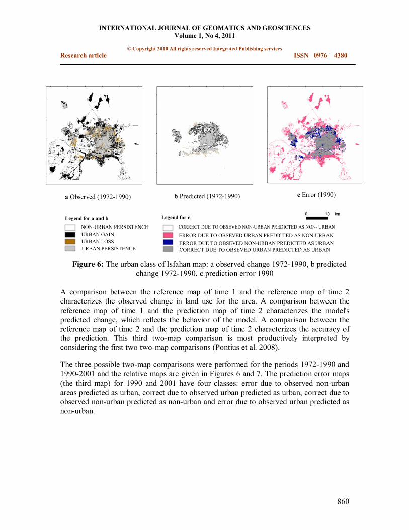
Figure 6: The urban class of Isfahan map: a observed change 19721990, b predicted change 19721990, c prediction error 1990
A comparison between the reference map of time 1 and the reference map of time 2 characterizes the observed change in land use for the area. A comparison between the reference map of time 1 and the prediction map of time 2 characterizes the model's predicted change, which reflects the behavior of the model. A comparison between the reference map of time 2 and the prediction map of time 2 characterizes the accuracy of the prediction. This third twomap comparison is most productively interpreted by considering the first two twomap comparisons (Pontius et al. 2008).
The three possible twomap comparisons were performed for the periods 19721990 and 19902001 and the relative maps are given in Figures 6 and 7. The prediction error maps (the third map) for 1990 and 2001 have four classes: error due to observed nonurban areas predicted as urban, correct due to observed urban predicted as urban, correct due to observed nonurban predicted as nonurban and error due to observed urban predicted as nonurban.
a Observed (19721990) b Predicted (19721990) c Error (1990)
Legend for a and b NONURBAN PERSISTENCE
URBAN PERSISTENCE
URBAN GAIN URBAN LOSS ERROR DUE TO OBSEVED NONURBAN PREDICTED AS URBAN
Legend for c
CORRECT DUE TO OBSEVED NONURBAN PREDICTED AS NON URBAN
ERROR DUE TO OBSEVED URBAN PREDICTED AS NONURBAN
CORRECT DUE TO OBSEVED URBAN PREDICTED AS URBAN

INTERNATIONAL JOURNAL OF GEOMATICS AND GEOSCIENCES Volume 1, No 4, 2011
© Copyright 2010 All rights reserved Integrated Publishing services Research article ISSN 0976 – 4380
861
Figure 7: The urban class of Isfahan map: a observed change 19902001, b predicted change 19902001, c prediction error 2001
5. Conclusion
Land cover mapping and change detection have increasingly been recognized as one of the most effective tools for environmental resource management. Isfahan and its environs are undergoing a fast, unplanned development, where urban area is growing without any consideration of the landscape types that are being transformed. If we suppose that processes like political policy, social and economical factors and also population factors which can change land cover and land use were constant across time, we would assume that model prediction results would be in agreement with past change trends. In the real world, these changes are not constant over long periods, so it is difficult to assume that future changes are the same as those which have gone before, potentially violating the Markov assumptions and therefore affecting the results of the predicting model. Finally, we can conclude that if processes of land cover change remain fixed and constant, CA Markov model predicts land cover changes with validation for the following years which agreement of predicted map with real map would be less than 70% for this study area.
6. References
1. Alphan H., Doygan H., and Unlukapman YI, (2008), Postclassification of land cover using multitemporal Landsat and ASTER imagery: the case of Kahramanmara, Turkey, Environmental Monitoring and Assessment, 10,pp 1 10.
Legend for a and b
NONURBAN PERSISTENCE
URBAN PERSISTENCE
URBAN GAIN URBAN LOSS ERROR DUE TO OBSEVED NONURBAN PREDICTED AS URBAN
Legend for c
CORRECT DUE TO OBSEVED NONURBAN PREDICTED AS NON URBAN
ERROR DUE TO OBSEVED URBAN PREDICTED AS NONURBAN
CORRECT DUE TO OBSEVED URBAN PREDICTED AS URBAN
a Observed (19902001) b predicted(19902001) c Error(2001)

INTERNATIONAL JOURNAL OF GEOMATICS AND GEOSCIENCES Volume 1, No 4, 2011
© Copyright 2010 All rights reserved Integrated Publishing services Research article ISSN 0976 – 4380
862
2. Ayodeji Opeyemi Z., (2006), Change detection in land use and land cover using remote sensing data and GIS, (A case study of Ilorin and its environs in Kwara State). The Department of Geography, University of Ibadan in Partial Fulfillment for the award of Master of Science.
3. Batty M., Couclelis H., and Eichen M, (1997), Urban system as cellular automata. Environment and Planning, 24(2),pp 159164.
4. Bell E.J, (1974), Markov analysis of land use change: an application of stochastic processes to remote sensed data, SocioEconomic Planning Sciences, 8,pp 311316.
5. Congalton, R.G, (1988), Using spatial autocorrelation analysis to explore the error in maps generated from remotely sensed data, Photogrammetric Engineering and remote sensing, 54,pp 587592.
6. Coppin P., Jonckheere I., Nackaerts K., and Muys B, (2004), Digital change detection methods in ecosystem monitoring: a review, International Journal Remote Sensing, 25,pp 15651596.
7. J.R.Estmen., (1995), Idrisi for windows user guide version 1/0. Clark University.
8. Chang C.L., and Chang, J.C, (2006), Markov model and cellular automata for vegetation, Journal of Geographical Research, 4,pp 4557.
9. Fan F., Wang Y., and Wang Z, (2008), Temporal and spatial change detecting (19982003) and predicting of land use and land cover in core corridor of Pearl River delta (China) by using TM and ETM + images, Environmental Monitoring and Assessment, 137,pp 127147.
10. Guindon B., Zhang Y., and Dillabaurgh, C, (2004), Landsat urban mapping based on a combined spectral spatial methodology, Remote sensing of environment, 92,pp 218232.
11. Hathout S, (2002), The use of GIS for monitoring and predicting urban growth in East and West St Paul, Winnipeg, Manitoba, Canada,. Journal of Environmental Management, 66,pp 229238.
12. Jahan S, (1986), The determination of stability and similarity of Markovian land use change processes: a theoretical and empirical analysis, Socio Economic Planning Sciences, 20,pp 243251.
13. Jensen J.R., and Cowen D.C, (1999), Remote sensing of urban suburban infrastructure and socioeconomic attributes, Photogrammetric Engineering and Remote Sensing, 65,pp 611622.

INTERNATIONAL JOURNAL OF GEOMATICS AND GEOSCIENCES Volume 1, No 4, 2011
© Copyright 2010 All rights reserved Integrated Publishing services Research article ISSN 0976 – 4380
863
14. Lambin E.F, (1997), Modeling and monitoring landcover change processes in tropical regions, Progress in phys. Geography, 21(3),pp 375393.
15. Lo´peza E., Bocco G., Mendoza M., and Duhau E, (2001), Predicting land cover and landuse change in the urban fringe: a case in Morelia city, Mexico, Landscape and Urban Planning, 55,pp 271285.
16. Parker D.C., Manson S.M., Janssen M.A., Hoffmann M.J., and Deadman, P, (2002), Multi agent systems for the simulation of land use and land cover change: a review, 43.
17. Pontius Jr R.G., and Schneider L.C, (2001), Landcover change model validation by an ROC method for the Ipswich watershed, Massachusetts, USA, Agriculture, Ecosystems and Environment, 85,pp 239248.
18. Pontius Jr R.G., Huffaker D., and Denman K, (2004), Useful techniques of validation for spatially explicit land change models. Ecological modeling, 179,pp 445461.
19. Pontius Jr R.G., and Spencer J, (2005), Uncertainty in extrapolations of predictive land cover models. Environment and Planning B: Planning and Design, 32,pp 211230.
20. Pontius Jr R.G., Boersma W., Castella J.C., Clarke K., Nijs, T.D., Dietzel C., (2008), Comparing the input, output, and validation maps for several models of land change, Annals of Regional Science, 42,pp 1137.
21. Rees W.G., Williams M., and Vitelosk P, (2003), Mapping land cover change in a reindeer herding area of the Russian arctic using Landsat TM and ETM+ imagery and indigenous knowledge, Remote sensing of environment, 85,pp 441452.
22. Robinson V.B, (1978), Information theory and sequences of land use: an application, The Professional Geographer, 30 (2), 174179.
23. Singh A, (1989), Digital change detection techniques using remotelysensed data, International Journal of Remote Sensing, 6,pp 9891003.
24. Schneider L.C., and Pontius JR R.G, (2001), Modeling land use change in the Ipswich watershed Massachusetts, USA, Agriculture, Ecosystems and Environment, 85,pp 8394.
25. Weng Q.H, (2002), Land use change analysis in the Zhujiang Delta of China using satellite remote sensing, GIS and stochastic modeling, Journal of Environment management, 64,pp 273284.

INTERNATIONAL JOURNAL OF GEOMATICS AND GEOSCIENCES Volume 1, No 4, 2011
© Copyright 2010 All rights reserved Integrated Publishing services Research article ISSN 0976 – 4380
864
26. Wijanarto A.B, (2006), Application of Markov change detection technique for detecting Landsat ETM derived land cover change over Banten Bay, Journal Ilmiah Geomatika, 12(1),pp 1121.
27. Wolfram S, (1984), Cellular automata as models of complexity, Nature, 31,pp 419424.
28. Wu Q., Li H.Q., Wang S., Paulussen J., He Y., Wang M., Wang B.H, and Wang, Z, (2006), Monitoring and predicting land use change in Beijing using remote sensing and GIS, Landscape and Urban Planning, 78,pp 322333.
29. Yang Q., Li X., Shi X, (2008), Cellular automata for simulating land use changes based on support vector machines, Computers & Geosciences, 34,pp 592602.