INTEGRATION OF TRIGENERATION AND CO2 BASED REFRIGERATION SYSTEMS

FOR ENERGY CONSERVATION

AA tthheessiiss ssuubbmmiitttteedd ffoorr tthhee ddeeggrreeee ooff DDooccttoorr ooff PPhhiilloossoopphhyy

By

I Nyoman Suamir, M.Sc.

DDeeppaarrttmmeenntt ooff MMeecchhaanniiccaall EEnnggiinneeeerriinngg SScchhooooll ooff EEnnggiinneeeerriinngg aanndd DDeessiiggnn

BBrruunneell UUnniivveerrssiittyy

SSeepptteemmbbeerr 22001122

ii

AABBSSTTRRAACCTT

Food retail with large supermarkets consumes significant amounts of energy. The environmental impact is also significant because of the indirect effect from CO2 emissions at the power stations and due to the direct effect arising from refrigerant leakage to the atmosphere. The application of trigeneration (local combined heat, power and refrigeration) can provide substantial improvements in the overall energy efficiency over the conventional supermarket energy approach of separate provision of electrical power and thermal energy.

The use of natural refrigerants such as CO2 offers the opportunity to reduce the direct impacts of refrigeration compared to conventional systems employing HFC refrigerants that possess high global warming potential. One approach through which the overall energy efficiency can be increased and the environmental impacts reduced, is through the integration of trigeneration and CO2 refrigeration systems where the cooling generated by the trigeneration system is used to condense the CO2 refrigerant in a cascade arrangement. This research project investigates experimentally and theoretically, through mathematical modelling and simulation, such a system and its potential application to supermarkets.

A small size CO2 refrigeration system for low and medium food temperature applications was designed and constructed to enable it to be integrated with an existing trigeneration system in the refrigeration laboratory at Brunel University to form an integrated trigeneration and CO2 refrigeration test facility. Prior to the construction, the design of the system was investigated using mathematical models developed for this purpose. The simulations included the CO2 refrigeration system, CO2 evaporator coils and the integration of the trigeneration and CO2 refrigeration systems. The physical size of the design and component arrangement was also optimised in a 3D AutoCAD model.

A series of experimental tests were carried out and the results showed that the medium temperature system could achieve a very good COP, ranging from 32 to 60 due to the low pumping power requirement of the liquid refrigerant. The low temperature system performed with average steady state COP of 4, giving an overall refrigeration system COP in the range between 5.5 and 6.

Mathematical models were also developed to investigate the application of the integrated trigeneration and CO2 refrigeration system in a case study supermarket. The models were validated against test results in the laboratory and manufacturers’ data. The fuel utilisation efficiency and environmental impacts of different trigeneration and CO2 refrigeration arrangements were also evaluated. The results indicated that a system comprising of a sub-critical CO2 refrigeration system integrated with a trigeneration system consisting of a micro-turbine based Combined Heat and Power (CHP) unit and ammonia-water absorption refrigeration system could provide energy savings of the order of 15% and CO2 emission savings of the order of 30% compared to conventional supermarket energy systems. Employing a trigeneration system with a natural gas engine based CHP and Lithium Bromide-Water sorption refrigeration system, could offer energy savings of 30% and CO2 emission savings of 43% over a conventional energy system arrangement. Economic analysis of the system has shown a promising payback period of just over 3 years compared to conventional systems.

iii

PPUUBBLLIICCAATTIIOONNSS

Published journal papers:

Suamir, IN., Tassou, S.A., Marriott, D., 2012. Integration of CO2 refrigeration and trigeneration systems for energy and GHG emission savings in supermarkets. Int. J. Refrigeration 35, 407-417.

Suamir, IN., Tassou, S.A., 2012. Performance evaluation of integrated trigeneration and CO2 refrigeration systems. Appl. Therm. Eng. doi:10.1016/j.applthermaleng. 2011. 11.055.

Published conference papers:

Suamir, IN., Tassou, S.A., 2011. Modelling and performance analyses of CO2 evaporator coils for chilled and frozen food display cabinets in supermarket applications. 23rd IIR International Congress of Refrigeration: Refrigeration for Sustainable Development, Prague, Czech Republic, ISBN 978-2-913149-89-2, paper no. 742, 8 pgs.

Suamir, IN., Tassou, S.A., 2011. Performance evaluation of integrated trigeneration and CO2 refrigeration systems. 2nd European Conference on Polygeneration, Tarragona, Spain, ISBN 978-8-461498-44-4, paper no. 47, 12 pgs.

Tassou, S.A., Suamir, IN., 2010. Trigeneration – a way to improve food industry sustainability. Proc. SEEP 2010 Conference, Bari, ITALY, 14 pgs.

Suamir, IN., Tassou, S.A., Hadawey, A., Marriott, D., 2010. Integration of CO2 refrigeration and trigeneration systems for supermarket application. Proc. 1st IIR Conference on Sustainability and the Cold Chain, Cambridge, UK, ISBN 978-2-9193149-75-5, paper no. 203, 8 pgs.

Suamir, IN., Tassou, S.A., Hadawey, A., Chaer, I., Marriott, D., 2009. Investigation of the performance characteristics of an ammonia-water absorption chiller in a trigeneration system arrangement. Proc. Heat and Power Cycle Conference, Berlin, Germany, ISBN 978-0-956332-90-5, paper no. HPC-430, 6 pgs.

Tassou, S.A., Chaer, I., Sugiartha, N., Marriott, D., Suamir, IN., 2008. Trigeneration - a solution to efficient use of energy in the food industry. Proc. Inst. R. 2007-08 7/1-16.

Other published conference papers:

Suamir, IN., Tassou, S.A., Arrowsmith, P., Bushell, M., 2012. Performance of integral hydrocarbon cabinets for supermarket applications. Proc. 10th IIR Gustav Lorentzen Conference on Natural Refrigerants, Delft, The Netherlands, ISBN 978-2-913149-90-8, paper no. GL-203, 8 pgs.

Hadawey, A., Tassou, S.A., Suamir, IN., Jouhara, H., 2010. Performance optimization of a secondary refrigerant display cabinet using tests and CFD modelling. Proc. 1st IIR International Cold Chain Conference, Cambridge, ISBN 978-2-913149-75-5, paper no. 214, 8 pgs.

Presented material:

Suamir, IN., Tassou, S.A., 2010. Trigeneration and its integration with CO2 refrigeration systems for supermarket applications. In: the SIRAC meeting, Brunel University, 23rd June 2010, 17 pgs, available from http://www.sirac.org.uk/.

iv

CCOONNTTEENNTTSS

AABBSSTTRRAACCTT ............................................................................................................................................................................................................................ iiii

PPUUBBLLIICCAATTIIOONNSS .......................................................................................................................................................................................................................... iiiiii

CCOONNTTEENNTTSS .......................................................................................................................................................................................................................... iivv

LLIISSTT OOFF FFIIGGUURREESS .............................................................................................................................................................................................................. vviiiiii

LLIISSTT OOFF TTAABBLLEESS .................................................................................................................................................................................................................... xxiiii

AACCKKNNOOWWLLEEDDGGEEMMEENNTTSS ...................................................................................................................................................................................... xxiiiiii

NNOOMMEENNCCLLAATTUURREE .............................................................................................................................................................................................................. xxiivv

AABBBBRREEVVIIAATTIIOONN AANNDD GGLLOOSSSSAARRYY .................................................................................................................................................. xxvviiii

CCHHAAPPTTEERR 11 IINNTTRROODDUUCCTTIIOONN ................................................................................................................................................................ 11 11..11 EEnneerrggyy ccoonnssuummppttiioonn ooff tthhee ffoooodd rreettaaiill iinndduussttrryy ........................................................................................................ 33 11..22 EEnnvviirroonnmmeennttaall iimmppaaccttss .................................................................................................................................................................................... 55 11..33 AApppprrooaacchh ttoowwaarrddss ssuussttaaiinnaabbiilliittyy ...................................................................................................................................................... 66 11..44 RReesseeaarrcchh pprroojjeecctt ddeessccrriippttiioonn .............................................................................................................................................................. 1100 11..55 RReesseeaarrcchh oobbjjeeccttiivveess .......................................................................................................................................................................................... 1122 11..66 SSttrruuccttuurree ooff tthhee tthheessiiss .................................................................................................................................................................................... 1133

CCHHAAPPTTEERR 22 CCOO22 RREEFFRRIIGGEERRAATTIIOONN IINN SSUUPPEERRMMAARRKKEETTSS .............................................................. 1144 22..11 CCOO22 aass rreeffrriiggeerraanntt ................................................................................................................................................................................................ 1155 22..22 DDiiffffeerreenntt ttyyppeess ooff CCOO22 rreeffrriiggeerraattiioonn ssyysstteemmss ............................................................................................................ 2211

2.2.1 Subcritical CO2 refrigeration systems ..................................................... 21 2.2.1.1 All-volatile systems ................................................................... 22 2.2.1.2 Volatile-DX system ................................................................... 25

2.2.2 All-CO2 systems ...................................................................................... 26 2.2.2.1 Parallel CO2 system arrangement .............................................. 27 2.2.2.2 Integrated CO2 system solutions ............................................... 28

22..33 SSuummmmaarryy .......................................................................................................................................................................................................................... 3322

CCHHAAPPTTEERR 33 DDEESSIIGGNN AANNDD CCOONNSSTTRRUUCCTTIIOONN OOFF TTHHEE TTEESSTT FFAACCIILLIITTYY .............. 3344 33..11 IInntteeggrraattiioonn aarrrraannggeemmeenntt ............................................................................................................................................................................ 3355 33..22 MMaatthheemmaattiiccaall mmooddeellss .................................................................................................................................................................................... 3366

3.2.1 Integration model ..................................................................................... 36 3.2.1.1 Trigeneration system model ...................................................... 36 3.2.1.2 CO2 refrigeration model ............................................................ 39 3.2.1.3 Integration capacity and performance simulations .................... 43

3.2.2 Piping system design and pressure drop simulation ................................ 53 3.2.3 EES model to determine the optimum size of the liquid receiver ........... 55 3.2.4 3D drawing of the CO2 refrigeration plant .............................................. 56

33..33 MMeecchhaanniiccaall ssyysstteemm ddeessiiggnn aanndd ccoommppoonneenntt sseelleeccttiioonn .................................................................................... 5588 3.3.1 CO2 compressor ....................................................................................... 60 3.3.2 CO2 pump ................................................................................................ 61 3.3.3 Condenser ................................................................................................ 62

v

3.3.4 Evaporators .............................................................................................. 63 3.3.5 Expansion valve ....................................................................................... 65 3.3.6 Internal heat exchanger ............................................................................ 66 3.3.7 Refrigerant flow control devices ............................................................. 67 3.3.8 Pressure relief valves ............................................................................... 68 3.3.9 Oil management system .......................................................................... 69 3.3.10 Auxiliary components ............................................................................. 70

33..44 RReeffrriiggeerraattiioonn llooaadd ssyysstteemm ........................................................................................................................................................................ 7722 3.4.1 Display cabinets ....................................................................................... 72 3.4.2 Low temperature additional load ............................................................. 73

33..55 CCoonnttrrooll ssyysstteemm .......................................................................................................................................................................................................... 7755 3.5.1 The electrical control system ................................................................... 75 3.5.2 The electronic control system .................................................................. 77 3.5.3 Control strategy ....................................................................................... 79

33..66 IInnssttrruummeennttaattiioonn aanndd ddaattaa llooggggiinngg ssyysstteemm ........................................................................................................................ 8822 3.6.1 Instrumentation devices ........................................................................... 82

3.6.1.1 Temperature and pressure measurements ................................. 82 3.6.1.2 Liquid level transducer .............................................................. 83 3.6.1.3 Relative humidity measurements .............................................. 84 3.6.1.4 Flow meter ................................................................................. 84 3.6.1.5 Power meter ............................................................................... 86 3.6.1.6 Velocity meter ........................................................................... 86

3.6.2 Data logging system ................................................................................ 87 33..77 RReeffrriiggeerraanntt cchhaarrggee .............................................................................................................................................................................................. 8888 33..88 EEnnvviirroonnmmeennttaall tteesstt cchhaammbbeerr ................................................................................................................................................................ 8899

3.8.1.1 Positioning the display cabinets in the test chamber ................. 91 3.8.1.2 Air handling unit ....................................................................... 91 3.8.1.3 Condensing unit ......................................................................... 93 3.8.1.4 Test chamber control system ..................................................... 94 3.8.1.5 Test chamber commissioning .................................................... 96

33..99 CCoommmmiissssiioonniinngg tthhee tteesstt ffaacciilliittyy ...................................................................................................................................................... 9977 33..1100 SSuummmmaarryy .......................................................................................................................................................................................................................... 9988

CCHHAAPPTTEERR 44 MMOODDEELLLLIINNGG AANNDD PPEERRFFOORRMMAANNCCEE AANNAALLYYSSEESS OOFF CCOO22 EEVVAAPPOORRAATTOORR CCOOIILLSS .......................................................................................................................................... 9999

44..11 IInnttrroodduuccttiioonn .................................................................................................................................................................................................................. 9999 44..22 EEvvaappoorraattoorr mmooddeell ddeessccrriippttiioonn ...................................................................................................................................................... 110000 44..33 MMaatthheemmaattiiccaall mmooddeell aapppprrooaacchh .................................................................................................................................................... 110022

4.3.1 Heat transfer coefficient and pressure drop at refrigerant side .............. 105 4.3.2 Heat transfer coefficient and pressure drop on the air side ................... 110 4.3.3 Calculation of frost accumulation ......................................................... 112 4.3.4 Overall surface efficiency of the evaporator coil .................................. 113

44..44 DDeessiiggnnss aanndd ppeerrffoorrmmaannccee ooff tthhee CCOO22 eevvaappoorraattoorr ccooiillss uuttiilliisseedd iinn tthhee MMTT aanndd LLTT ccaabbiinneettss ooff tthhee tteesstt rriigg ...................................................................................................................................................... 111144

44..55 EExxppeerriimmeennttaall aanndd tthheeoorreettiiccaall vvaalliiddaattiioonn ooff tthhee mmooddeellss .......................................................................... 111177 44..66 PPeerrffoorrmmaannccee aannaallyysseess ooff CCOO22 eevvaappoorraattoorr ccooiillss .................................................................................................. 111188 44..77 SSuummmmaarryy ...................................................................................................................................................................................................................... 112211

CCHHAAPPTTEERR 55 EEXXPPEERRIIMMEENNTTAALL TTEESSTT RREESSUULLTTSS AANNDD MMOODDEELL VVAALLIIDDAATTIIOONN .................................................................................................................................................................. 112222

vi

55..11 OOvveerrvviieeww ooff tthhee aass--bbuuiilltt tteesstt ffaacciilliittyy .................................................................................................................................. 112222 55..22 EExxppeerriimmeennttaall tteesstt ccoonnddiittiioonnss aanndd ddaattaa pprroocceessssiinngg .......................................................................................... 112255

5.2.1 Test conditions....................................................................................... 125 5.2.2 Experimental test procedure .................................................................. 125 5.2.3 Operational setting ................................................................................. 126 5.2.4 Data collection ....................................................................................... 126 5.2.5 Data processing ..................................................................................... 126

5.2.5.1 Calculation of the refrigeration capacity ................................. 127 5.2.5.2 Power consumption ................................................................. 127 5.2.5.3 Calculation of the COP ........................................................... 128 5.2.5.4 Circulation ratio ....................................................................... 128 5.2.5.5 Uncertainty in the calculation of CR and COP ....................... 129

55..33 TTeesstt rreessuullttss .................................................................................................................................................................................................................. 113300 5.3.1 Thermodynamic cycle of the refrigeration system ................................ 130 5.3.2 Medium temperature refrigeration system ............................................ 131 5.3.3 Low temperature refrigeration system ................................................... 133 5.3.4 Overall refrigeration system .................................................................. 134 5.3.5 Product and air temperatures ................................................................. 135 5.3.6 Frost performance of the CO2 display cabinets ..................................... 140

55..44 VVaalliiddaattiioonn ooff tthhee aannaallyyttiiccaall rreessuullttss ........................................................................................................................................ 114422 55..55 SSuummmmaarryy ...................................................................................................................................................................................................................... 114444

CCHHAAPPTTEERR 66 AANNAALLYYSSIISS OOFF TTHHEE IINNTTEEGGRRAATTEEDD SSYYSSTTEEMM IINN AA SSUUPPEERRMMAARRKKEETT AAPPPPLLIICCAATTIIOONN:: AA CCAASSEE SSTTUUDDYY AAPPPPRROOAACCHH .......................................................................................................................................................................... 114466

66..11 TThhee ccaassee ssttuuddyy ssuuppeerrmmaarrkkeett ............................................................................................................................................................ 114466 66..22 SSuuppeerrmmaarrkkeett eenneerrggyy ssyysstteemm aanndd ssiimmuullaattiioonn mmooddeellss .................................................................................. 114499 66..33 EEnneerrggyy ppeerrffoorrmmaannccee ooff tthhee ccoonnvveennttiioonnaall ssyysstteemm ............................................................................................ 115544 66..44 EEnneerrggyy aanndd eennvviirroonnmmeennttaall ppeerrffoorrmmaannccee ooff tthhee ttrriiggeenneerraattiioonn--

CCOO22 rreeffrriiggeerraattiioonn ssyysstteemm ...................................................................................................................................................................... 115555 66..55 SSuummmmaarryy ...................................................................................................................................................................................................................... 115577

CCHHAAPPTTEERR 77 EENNEERRGGYY SSYYSSTTEEMM AALLTTEERRNNAATTIIVVEESS WWIITTHH IINNTTEEGGRRAATTEEDD TTRRIIGGEENNEERRAATTIIOONN AANNDD CCOO22 RREEFFRRIIGGEERRAATTIIOONN ................................................ 115588

77..11 SSuuppeerrmmaarrkkeett eenneerrggyy ssyysstteemm aalltteerrnnaattiivveess ...................................................................................................................... 115588 77..22 SSiimmuullaattiioonn mmooddeellss .......................................................................................................................................................................................... 116633 77..33 MMooddeell rreessuullttss aanndd ddiissccuussssiioonn .......................................................................................................................................................... 116655 77..44 EEccoonnoommiicc aannaallyyssiiss .......................................................................................................................................................................................... 116699 77..55 SSuummmmaarryy ...................................................................................................................................................................................................................... 117711

CCHHAAPPTTEERR 88 CCOONNCCLLUUSSIIOONNSS AANNDD RREECCOOMMMMEENNDDAATTIIOONNSS FFOORR FFUUTTUURREE WWOORRKK ............................................................................................................................................................ 117722

88..11 CCoonncclluussiioonnss .............................................................................................................................................................................................................. 117733 88..22 RReeccoommmmeennddaattiioonnss ffoorr ffuuttuurree wwoorrkk ........................................................................................................................................ 117799

RREEFFEERREENNCCEESS .................................................................................................................................................................................................................... 118811

AAppppeennddiixx AA:: TTrriiggeenneerraattiioonn ppllaanntt ........................................................................................................................................................ 118899

AAppppeennddiixx BB:: MMaatthheemmaattiiccaall mmooddeell ooff iinntteeggrraatteedd ttrriiggeenneerraattiioonn aanndd CCOO22 rreeffrriiggeerraattiioonn ............................................................................................................................................................................ 119900

AAppppeennddiixx CC:: MMeecchhaanniiccaall ccoommppoonneennttss ...................................................................................................................................... 119955

vii

AAppppeennddiixx DD:: EElleeccttrriiccaall cciirrccuuiitt ddiiaaggrraammss ooff tthhee CCOO22 tteesstt ssyysstteemm ...................................................... 220022

AAppppeennddiixx EE:: IInnssttrruummeennttaattiioonn aanndd ddaattaa llooggggiinngg ssyysstteemmss ................................................................................ 221111

AAppppeennddiixx FF:: CCOO22 tteesstt cchhaammbbeerr ............................................................................................................................................................ 222211

AAppppeennddiixx GG:: OOppeerraattiioonnaall mmooddeess aanndd pprroocceedduurreess ...................................................................................................... 222299

AAppppeennddiixx HH:: MMaatthheemmaattiiccaall mmooddeell ooff CCOO22 eevvaappoorraattoorr ccooiillss .................................................................... 223355

AAppppeennddiixx II:: AAss bbuuiilltt iinntteeggrraatteedd ttrriiggeenneerraattiioonn aanndd CCOO22 rreeffrriiggeerraattiioonn ...................................... 223399

AAppppeennddiixx JJ:: UUnncceerrttaaiinnttyy aannaallyyssiiss .................................................................................................................................................... 224400

AAppppeennddiixx KK:: RReeffrriiggeerraanntt cchhaarrggee aanndd lleeaakk rraattee .............................................................................................................. 224444

AAppppeennddiixx LL:: EEEESS mmooddeellss ooff tthhee rreeffrriiggeerraattiioonn ssyysstteemmss ffoorr tthhee ccoonnvveennttiioonnaall aanndd ttrriiggeenneerraattiioonn –– CCOO22 rreeffrriiggeerraattiioonn eenneerrggyy ssyysstteemmss ............................................ 224455

AAppppeennddiixx MM:: DDeettaaiilleedd aannaallyyssiiss ooff eenneerrggyy aanndd eennvviirroonnmmeenntt ppeerrffoorrmmaannccee ooff tthhee ccoonnvveennttiioonnaall aanndd ttrriiggeenneerraattiioonn –– CCOO22 rreeffrriiggeerraattiioonn eenneerrggyy ssyysstteemmss ............................................................................................................................................................................................ 224488

AAppppeennddiixx NN:: DDeettaaiilleedd aannaallyyssiiss ooff eenneerrggyy aanndd eennvviirroonnmmeenntt ppeerrffoorrmmaannccee ooff tthhee eenneerrggyy ssyysstteemm aalltteerrnnaattiivveess ................................................................................................................................ 225500

AAppppeennddiixx OO:: AAssssuummppttiioonnss ffoorr tthhee eeccoonnoommiicc aannaallyyssiiss ...................................................................................... 225533

viii

LLIISSTT OOFF FFIIGGUURREESS

Figure 1.1 Cold chain and refrigeration technology in the life cycle stages of food products ............................................................................................... 2

Figure 1.2 Annual electricity consumption of typical 50,000 ft2 UK supermarket ...... 4 Figure 1.3 Electricity consumption of refrigeration packs and display cabinets

of some F-50 supermarkets in the UK ......................................................... 5 Figure 1.4 Efficiency of different module types of gas engine based CHP .................. 7 Figure 1.5 Comparison of electricity and gas price in the UK ...................................... 9 Figure 2.1 CO2 expansion and phase change .............................................................. 16 Figure 2.2 Liquid and gas pressure-drop ratio for selected refrigerants and CO2

at different saturated temperatures, investigated at the same operating conditions ................................................................................... 18

Figure 2.3 Acceptable pressure drop for CO2 and selected refrigerants in gas and liquid lines of a refrigeration system ................................................... 19

Figure 2.4 Schematic diagram of a cascade arrangement using CO2 as the low stage cycle .................................................................................................. 22

Figure 2.5 Parallel MT and LT indirect system with CO2 as secondary fluid ............ 23 Figure 2.6 All-volatile CO2 subcritical system with LT DX circuit ........................... 24 Figure 2.7 Cascade CO2 refrigeration with MT secondary loop and LT DX

system ........................................................................................................ 25 Figure 2.8 COP of a CO2 transcritical cycle vs. pressures of the gas cooler at

different exit gas temperatures ................................................................... 27 Figure 2.9 Simplified parallel CO2 refrigeration systems ........................................... 28 Figure 2.10 All-CO2 booster system with gas bypass ................................................... 29 Figure 2.11 All-CO2 booster system installed in the Refrigeration Laboratory,

Brunel University ....................................................................................... 29 Figure 2.12 Integrated cascade all-CO2 system with flash gas bypass ......................... 30 Figure 2.13 Integrated cascade all-CO2 system with suction receiver .......................... 31 Figure 2.14 Integrated cascade all-CO2 plant in Tesco Ramsey, UK ........................... 32 Figure 3.1 Integration arrangement of CO2 refrigeration and trigeneration

systems ....................................................................................................... 35 Figure 3.2 Schematic diagram of the microturbine based CHP system ...................... 37 Figure 3.3 Schematic diagram of the ammonia-water absorption chiller ................... 38 Figure 3.4 Centralised volatile-DX CO2 section ......................................................... 40 Figure 3.5 P-h diagram of the subcritical CO2 refrigeration cycle .............................. 41 Figure 3.6 A simplified schematic diagram of the integrated arrangement

displayed in the model ............................................................................... 44 Figure 3.7 Effect of the ambient temperature on the COP of the absorption and

integrated systems ...................................................................................... 46 Figure 3.8 Seasonal performance of the absorption and the integrated systems ......... 46 Figure 3.9 Variation of system COP with condensing temperature ............................ 47 Figure 3.10 Variation of system COP with LT evaporating temperature ..................... 48 Figure 3.11 Variation of COP with load ratio of LT and MT systems ......................... 49 Figure 3.12 Variation of superheating, subcooling and COPLT with different IHX

effectiveness ............................................................................................... 50

44

ix

Figure 3.13 Effect of circulation ratio (CR) on the COP, refrigeration duty and power consumption of the MT refrigeration system ................................. 51

Figure 3.14 Effect of the circulation ratio (CR) on the overall COPs of the CO2 system and the integrated arrangement ...................................................... 52

Figure 3.15 Simulation results from liquid receiver model .......................................... 55 Figure 3.16 The liquid receiver ...................................................................................... 56 Figure 3.17 The subcritical CO2 refrigeration test plant in a 3D drawing ..................... 57 Figure 3.18 Piping diagram of the integrated CO2 refrigeration and trigeneration

system ........................................................................................................ 59 Figure 3.19 CO2 compressor with specified performance data ..................................... 61 Figure 3.20 CO2 pump .................................................................................................. 62 Figure 3.21 CO2 condenser ........................................................................................... 63 Figure 3.22 MT CO2 evaporator coils fitted in the display cabinet .............................. 64 Figure 3.23 Electronic expansion valve ........................................................................ 65 Figure 3.24 Performance data of electronic expansion valves type AKV10 ................ 66 Figure 3.25 Internal heat exchanger .............................................................................. 66 Figure 3.26 Refrigerant flow control valves ................................................................. 67 Figure 3.27 Pressure relief valve and its discharge capacity ........................................ 68 Figure 3.28 Schematic diagram and selected components of the oil management

system ........................................................................................................ 69 Figure 3.29 The auxiliary components .......................................................................... 71 Figure 3.30 Refrigerated display cabinets ..................................................................... 73 Figure 3.31 Schematic diagram of the LT additional load ............................................ 74 Figure 3.32 Schematic diagram of the electrical and electronic control systems ......... 76 Figure 3.33 Control components ................................................................................... 78 Figure 3.34 Electrical control panel .............................................................................. 79 Figure 3.35 Operational control strategy ....................................................................... 81 Figure 3.36 Liquid level transducer and the electrical connections to controller ........ 84 Figure 3.37 Flow meter of the LT, MT and additional load systems ............................ 85 Figure 3.38 Power meter, Voltech PM-300 .................................................................. 86 Figure 3.39 Data logging system ................................................................................... 87 Figure 3.40 CO2 and charging connection .................................................................... 88 Figure 3.41 CO2 test chamber and associated test facilities .......................................... 89 Figure 3.42 Technical walls of the CO2 test chamber ................................................... 90 Figure 3.43 Position of the MT and LT cabinets in the test chamber ........................... 91 Figure 3.44 Schematic diagram of the air handling unit and font view of the test

chamber ...................................................................................................... 92 Figure 3.45 Schematic diagram of the test chamber control system ............................. 95 Figure 3.46 Variation of the test chamber conditions and ambient temperatures ......... 96 Figure 4.1 Structure of the simulation models for flooded and DX evaporator

coils .......................................................................................................... 101 Figure 4.2 Geometry of a finned tube evaporator model .......................................... 102 Figure 4.3 Schematic of flooded and DX evaporator coils with single and two

control volumes respectively ................................................................... 103 Figure 4.4 A flow pattern map of CO2 evaporation inside DX and flooded

evaporator coils ........................................................................................ 106 Figure 4.5 Variation of CO2 two phase heat transfer coefficient and pressure

drop .......................................................................................................... 108

59

65

76

86

66

x

Figure 4.6 Comparison of two phase heat transfer coefficient and pressure drop between CO2 and R-404A ........................................................................ 109

Figure 4.7 The influence of circulation ratio (CR) and evaporating temperatures on the flooded coil capacity and refrigerant mass flow rate .................... 116

Figure 4.8 Refrigerant charge comparisons .............................................................. 119 Figure 4.9 The influence of evaporating temperature on the performance of MT

DX coils ................................................................................................... 119 Figure 4.10 The influence of circulation ratio on the performance of the flooded

coils .......................................................................................................... 120 Figure 5.1 Simplified diagram of the integrated volatile-DX CO2 refrigeration

and trigeneration ...................................................................................... 123 Figure 5.2 Retail refrigeration system module with CO2 refrigeration system ......... 124 Figure 5.3 Pressure-enthalpy diagram of the CO2 refrigeration cycle based on

the test results ........................................................................................... 130 Figure 5.4 Variation of MT refrigeration capacity and COP with circulation

ratio for different evaporating temperatures ............................................ 131 Figure 5.5 Performance of the CO2 MT refrigeration system ................................... 132 Figure 5.6 Performance of the CO2 LT refrigeration system .................................... 133 Figure 5.7 Evaporation and condensing temperatures including theoretical COP

of the LT system ...................................................................................... 134 Figure 5.8 Performance of the CO2 MT and LT refrigeration systems ..................... 135 Figure 5.9 Variation of the MT product temperatures with time .............................. 135 Figure 5.10 Positions of the product temperature measurements for the MT

cabinet ...................................................................................................... 136 Figure 5.11 Variation of air temperatures and RHs of the MT cabinet ...................... 137 Figure 5.12 Variation of the LT product temperatures with time ............................... 138 Figure 5.13 Positions of the product temperature measurements for the LT

cabinet ...................................................................................................... 139 Figure 5.14 Variation of air temperatures and RHs of the LT cabinet ........................ 140 Figure 5.15 MT evaporator coil with frost accumulations and without frost ............. 141 Figure 5.16 Predicted and experimental frost accumulation on the flooded MT

evaporator coil for 4 hours defrost cycles ................................................ 141 Figure 5.17 Isentropic efficiency of the LT compressor ............................................. 142 Figure 5.18 Comparison between the predicted and actual COP of the MT

system ...................................................................................................... 143 Figure 5.19 Comparison between the predicted and actual COP of the LT system ... 143 Figure 5.20 Comparison between the predicted and actual overall COP of the

CO2 system .............................................................................................. 144 Figure 6.1 The case study supermarket ..................................................................... 146 Figure 6.2 Daily average of the energy consumption rate of the case study

supermarket .............................................................................................. 147 Figure 6.3 Daily average energy rate demand of the case study supermarket .......... 148 Figure 6.4 Daily average electrical-energy rate demand of all services apart

from refrigeration systems ....................................................................... 149 Figure 6.5 Energy flow diagram of the case study supermarket with a

conventional energy system ..................................................................... 150 Figure 6.6 Simplified schematic diagram of a parallel conventional refrigeration

system with R-404A refrigerant .............................................................. 150

146

xi

Figure 6.7 Energy flow diagram of the case study supermarket with energy system applying a volatile-DX CO2 refrigeration in trigeneration arrangement ............................................................................................. 151

Figure 6.8 Daily average fuel utilisation ratio of the conventional energy system ... 155 Figure 6.9 Daily average fuel energy utilisation ratio of the trigeneration-CO2

energy system .......................................................................................... 156 Figure 7.1 Energy flow diagram of existing energy system (Scheme-1) .................. 159 Figure 7.2 Simplified schematic diagram of a cascade transcritical CO2

refrigeration integrated with trigeneration system (Scheme-2) ............... 160 Figure 7.3 Simplified schematic diagram of integrated trigeneration and CO2

refrigeration systems (Scheme-3) ............................................................ 161 Figure 7.4 Energy flow diagram of energy system alternatives ................................ 162 Figure 7.5 Thermodynamic models of the refrigeration system of Schemes 1 to

3 at ambient temperature of 27 oC ........................................................... 164 Figure 7.6 Daily average fuel energy utilisation ratio of scheme-1 .......................... 165 Figure 7.7 Daily average fuel energy utilisation ratio of scheme-2 .......................... 166 Figure 7.8 Daily average fuel energy utilisation ratio of scheme-3 .......................... 168 Figure 7.9 Variation of payback period with spark ratio .......................................... 170

xii

LLIISSTT OOFF TTAABBLLEESS

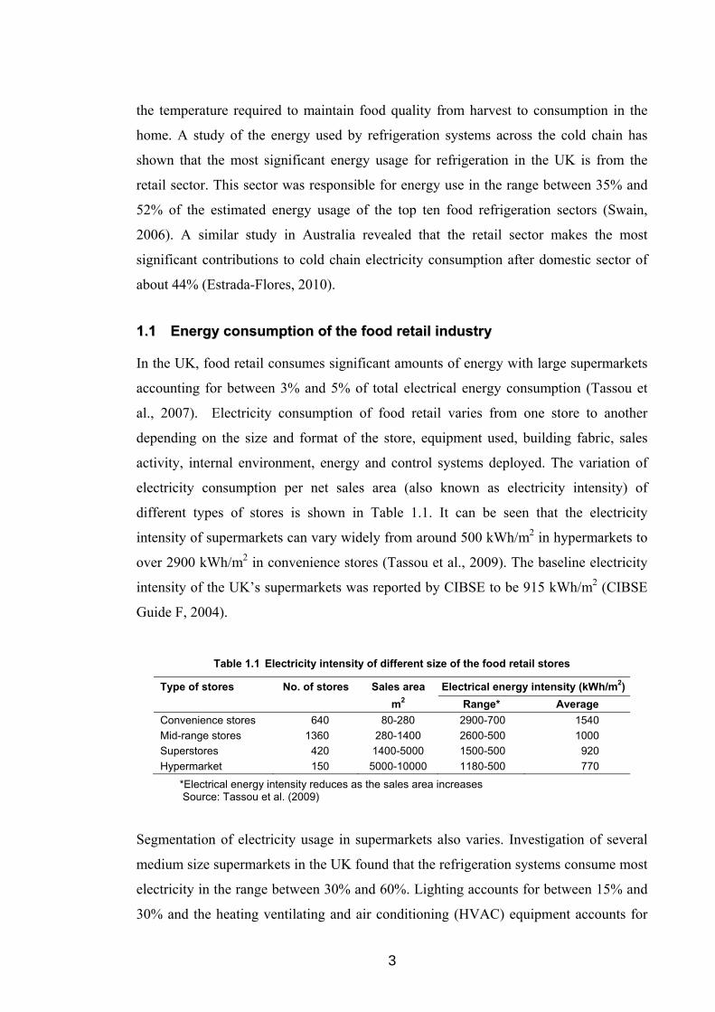
Table 1.1 Electricity intensity of different size of the food retail stores ........................ 3 Table 2.1 Comparative refrigerant performance per kW for MT and

LT refrigeration ............................................................................................ 17 Table 2.2 Price comparison of selected refrigerants .................................................... 19 Table 3.1 Constants of the best fit equations ............................................................... 38 Table 3.2 Equations for the CO2 refrigeration system ................................................. 42 Table 3.3 Design conditions and estimated performance parameters .......................... 52 Table 3.4 Specified pipe sizes of the CO2 refrigeration system ................................... 54 Table 4.1 Equations for the thermal resistance of the coil ......................................... 105 Table 4.2 Key equations for two phase heat transfer coefficient and

pressure drop for CO2 inside a horizontal tube .......................................... 107 Table 4.3 Design parameters of the evaporator coils ................................................. 114 Table 4.4 Coil geometry and estimated performance parameters .............................. 115 Table 4.5 Model and experimental results ................................................................. 117 Table 4.6 Geometry of the designed coils and their performance parameters ........... 118 Table 5.1 Operational setting of the MT and LT cabinets and the additional load

evaporator ................................................................................................... 126 Table 5.2 Mean, maximum and minimum temperatures of the MT products............ 137 Table 5.3 Mean, maximum and minimum temperatures of the LT products ............. 139 Table 5.4 Statistical analysis of the predicted COP of the CO2 refrigeration system 144 Table 6.1 Assumptions for TEWI calculation of the case study supermarket ........... 154 Table 6.2 Fuel saving analysis of conventional and trigeneration-CO2

energy systems ........................................................................................... 157 Table 6.3 CO2e emissions of conventional and trigeneration-CO2 energy systems .. 157 Table 7.1 Results of fuel energy saving analysis ....................................................... 168 Table 7.2 CO2e emissions of investigated energy systems ........................................ 169 Table 7.3 Results of economic analysis: investment comparison .............................. 169 Table 7.4 Results of economic analysis: annual energy and operational cost ........... 170

19

xiii

AACCKKNNOOWWLLEEDDGGEEMMEENNTTSS

Integration of trigeneration and CO2 based refrigeration systems for energy conservation in the food industry was a research project in the Centre for Energy and Built Environment Research (CEBER), School of Engineering and Design, Brunel University. The project was managed by Prof. Savvas Tassou and financially supported by DEFRA under the Advanced Food Manufacturing LINK Programme. This thesis is based on the work carried out for this project.

I am really grateful for the opportunity to be the researcher on this project. The project has appreciably broadened my knowledge and has considerably improved my practical skill and research experience in the areas of CO2 refrigeration and trigeneration.

I would like to express my special appreciation and gratitude to Prof. Savvas Tassou for his guidance and enthusiastic support throughout the project. His advice and encouragement have strongly inspired me to complete the project successfully and this thesis. I would also like to thank Dr. Yunting Ge, a member of the academic team, for his assistance as well as the refrigeration laboratory technical team and all my colleagues in the Mechanical Engineering Department of Bali State Polytechnic for all their support and encouragement.

It is my great pleasure to acknowledge the financial support received from the Food Technology Unit of DEFRA and the contribution of the industrial collaborators: Tesco Stores Ltd, A&N Shilliday & Company Ltd, ACDP (Integrated Building Services) Ltd, Apex Air Conditioning Ltd, Bock Kältemaschinen GmbH, the Bond Group, Bowman Power group, Cambridge Refrigeration Technology, Cogenco, CSA Consulting Engineers Ltd, Danfoss, Doug Marriott Associates, George Baker & Co (Leeds) Ltd and Somerfield Property Co Ltd.

Finally, I would like to express my very special gratitude to my wife, Ni Made Kuerti, and my daughters, Ni Wayan Engginia and Ni Made Ticheyani, for their patience and fortitude during the most arduous time. I would like to dedicate my thesis to them. I also express my gratitude to my parents and relatives for their support and encouragement.

xiv

NNOOMMEENNCCLLAATTUURREE

A Area (m2) COP Coefficient of performance (-) Cp Specific heat (kJ/kg.K) CR Circulation ratio (-): defined as the ratio of refrigerant mass flow

rate circulated through the evaporator to the mass flow rate of refrigerant vaporised, described in page 50 and equation (5.6)

d Diameter (m or mm) Dh Hydraulic diameter at air side of a finned tube coil (m) Ef Fuel energy consumption (kWh) Eannual Energy consumption (kWh) FESR Fuel energy saving ratio (%) FEUR Fuel energy utilization ratio (%) Fo Fourier number (-) G mass velocity (kg/s.m2) GWP Global warming potential (kgCO2/kg) H Specific enthalpy (kJ/kg) h Heat transfer coefficient (kW/m2.K or W/m2.K) j Colburn j-factor (-) L Length (m) Lannual Annual refrigerant leakage (kg) mcharge Mass of refrigerant charge (kg) m Mass (kg); a fin efficiency parameter (1/m) defined by

equation (4.33) m mass flow rate (kg/s) M Molecular weight (kg/mol) n System operating time (years) N Number of rows or circuits NPSH Net positive suction head (mLC: metre liquid column) P Pressure (kPa or Pa or bar or bara) Pr Prandtl number (-) Q Discharge capacity (kg/h); heating or refrigerating load (kW or

kWh) q Heat flux (W/m2) R Thermal resistance (m2.K/kW) Re Reynolds number (-) RH Relative Humidity (%) Rp Pressure ratio (-) S Suppression factor (-), spacing (m) T Temperature (oC or K) t Time (s) u Refrigerant velocity (m/s)

xv

U Overall heat transfer coefficient (kW/m2.K) W Electrical power/energy (kW or kWh) x Vapour quality (-) Greek symbols α Recovery factor; thermal diffusivity (m2/s) β CO2 emissions factor (kgCO2/kWh) ∆ Difference δ Thickness (m or mm), liquid film thickness (m) ε Cross sectional vapour void fraction (-) φ Density of heat flowrate (kW/m2) η Efficiency λ Thermal conductivity (kW/m.K or W/m.K) μ Dynamic viscosity (N.s/m2) ρ Density (kg/m3) θ Dry angle (rad) Fin efficiency parameter (-) defined by equation (4.34) ω Humidity ratio (kg/kgda) Subscript a Air or air-side abs Absorption chiller add Additional load amb Ambient c Cooling, convective, circuit, cold cab Display cabinet cb Convective boiling ChW Chilled water comp Compressor cond Condensing, condenser conv Conventional crit Critical point CW Cooling water d Diagonal de Dry out completion df Defrost cycle Dh Calculated at hydraulic diameter di dry out inception e Electrical eq Equivalent evap Evaporating, evaporator f Fin or fuel ff Free flow sectional fl Fouling fr Frictional

xvi

H Homogenous h Heating, hydraulic, hot htf Heat transfer fluid i Inlet, in, width axis int Integrated system, intermediate j Depth axis k Height axis L Liquid phase lat Latent lm Logarithmic mean m Mean, momentum M Mist flow region md Maximum discharge nb Nucleate boiling o Outlet, out, overall others Other than refrigeration and electric chiller r Refrigeration, refrigerant, refrigerant-side SG Standby generator sp Single phase s Isentropic, surface sc Sub-cooling sh Superheating t Tube th Thermal tp Two phase tri Trigeneration trigen integrated trigeneration and CO2 refrigeration energy system trip Triple point V Vapour phase v Volumetric vap Vaporization w Water-glycol mixture

xvii

AABBBBRREEVVIIAATTIIOONN AANNDD GGLLOOSSSSAARRYY

AK-CC Adap-Kool cabinet controller: a cabinet controller manufactured by Danfoss

AKV Adap-Kool valve: an electrically operated expansion valve manufactured by Danfoss

ARI Air conditioning and refrigeration institute

ASHRAE American society of heating refrigerating and air-conditioning engineers

BV Ball valve

CCC Committee of the climate change

CCHP Combined cooling heating and power

CFC Chloro-fluoro-carbon

CHRP Combined heating refrigeration and power

CHP Combined heat and power

CIBSE Chartered Institution of building services engineers

CO2 Carbon dioxide

CO2e Carbon dioxide equivalent

CP grade Chemically pure

DEFRA Department for environment, food and rural affairs

EES Engineering equation solver

EC Evaporator coil

EIA Energy information administration

ETS Electrically operated expansion valve, manufactured by Danfoss

EXV Electronic expansion valve

DX Direct expansion

FPI Number of fins per inch

FPM Number of fins per metre

Fossil fuel An energy source formed in the earths crust from decayed organic material. The common fossil fuels are petroleum, coal and natural gas.

Food refrigeration Application of a refrigeration system on the prevention and retardation of microbial, physiological, and chemical changes in foods. It also plays a major role in maintaining a safe food supply, nutritional content and retaining characteristics such as flavour, colour and texture (ASHRAE, 2010)

GHG Green House Gases: gaseous constituents of the atmosphere, both natural and anthropogenic, that absorb and emit radiation at specific wavelengths within the spectrum of infrared radiation emitted by the Earth's surface, the atmosphere, and clouds (PAS 2050, 2008)

xviii

GAX Generator absorber heat exchange

HC Hydrocarbon

HCFC Hydro-chloro-fluoro-carbon

HFC Hydro-fluoro-carbon

HT High stage of a cascade system/High temperature

HTF Heat transfer fluid

HVAC Heating ventilation and air conditioning

HX Heat exchanger

ICM Industrial control motor valve

ICMT High pressure expansion valve

IHX Internal heat exchanger

IEA International energy agency

IPCC Intergovernmental panel on climate change

Isenthalpic expansion Expansion which takes place without any change in enthalpy

kW Kilowatt

kWh Kilowatt hour

LRLM Load ratio low to medium temperatures of a refrigeration plant

LT Low temperature

MO Mineral oil

MOP Maximum operating pressure

MOPD Maximum operating pressure difference

MT Medium temperature

MTP Market transformation programme

MWh Megawatt hour = 1000 kilowatt hour

N/A Not applicable

NG Natural Gas (primarily methane)

NRV Non-return valve

O&M Operational and maintenance

ODP Ozone depleting potential

PAO Poly-alpha olefin (oil)

PAS Publicly available specification

PHX Plate type heat exchanger

POE Polyol ester (oil)

Primary fuel All fuels consumed by end users, including the fuel consumed at electric utilities to generate electricity

ppm Part per million

PTC Positive temperature coefficient

Refrigerated display cabinet: a cabinet cooled by a refrigerating system which enables chilled and frozen foodstuffs placed therein for display to be maintained within prescribed temperature limits (ISO 23953-1, 2005)

xix

RCD Residual current device

RV Regulator valve

SCA Solution cooled absorber

SG Sight glass

SRC Specific refrigerant charge defined as refrigerant mass per unit refrigerating capacity, or heating capacity for heat pumps (MTP, 2008); Super radiator coils

SV Solenoid valve

Sustainability Sustainable development is development that meets the needs of the present without compromising the ability of future generations to meet their own needs (Evans, 2010)

TOC Technical options Committee (UNEP)

TXV Thermostatic expansion valve

Uncertainty A concept to describe the degree of goodness of a measurement, experimental result, or analytical result (Coleman and Steele, 2009); lack of confidence

UNEP United Nations Environment Programme

1

CChhaapptteerr 11

IINNTTRROODDUUCCTTIIOONN

Global energy demand has been increasing alongside the growth of world population

and economy. The increase of energy demand, especially energy from fossil fuel,

increases emissions to atmosphere which contributes to the deterioration of ambient air

quality with serious public health and environmental effects. World energy demand

related greenhouse gas emissions, on the basis of current policies, will be 40% higher in

the year 2030 relative to 2007 (IEA, 2009). In order to deal with increases in fossil fuel

use, industrialised countries such as the UK and the European Union have been

developing an ambitious energy policy to tackle carbon dioxide emissions and climate

change. In the UK, the targets are a 60% reduction in greenhouse gas emissions by

2030 compared to 1990 levels and a reduction of at least 80% by 2050 (CCC, 2008 and

CCC, 2010).

In developed countries, there is also a trend of increasing consumption of food products

which in them has an impact on greenhouse gas emissions. It is estimated that for

Western Europe the food industry is responsible for between 20% and 30% of GHG

emissions (Tassou and Suamir, 2010). A major source of emissions is energy use by

manufacturing processes, food distribution and retail. In the UK, food distribution and

retail are responsible for approximately 7% of total GHG emissions (DEFRA, 2005).

Refrigeration, which is increasingly important in the processing and preservation of

food, is potentially responsible for significant GHG emissions. As described by

Coulomb (2008), refrigeration technology is responsible for 15% of all electricity

consumed worldwide. Approximately 72% of the global warming impact of

2

refrigeration plant is due to energy consumption (Cowan et al., 2010). Reducing the

energy consumption of refrigeration plant has therefore become one of the key priorities

in the reduction of GHG emissions of the food sector.

Another important source of GHG emissions from refrigeration is refrigerant leakage

from the refrigeration plant. Extensive pipe-work with associated pipe joints used in

refrigeration plant increases the potential for refrigerant losses. HFC refrigerants,

currently used in food refrigeration systems, have zero impact on ozone depletion

(ODP) and provide comparable performance to CFC and HCFC refrigerants. Leakage of

HFC refrigerants to the atmosphere, however, has significant impact on GHG emissions

due to their high global warming potential (GWP). This has prompted the introduction

of the F-gas regulations by the European Union which are designed to contain, prevent

and thereby reduce emissions of fluorinated gases including all HFC refrigerants, such

as R-134A, R-407C, R-410A, and R-404A. Replacement of F-gas based refrigerants

with negligible or no GWP refrigerants (often called ‘natural refrigerants’) such as

hydrocarbons, ammonia and CO2 can reduce direct impacts to the environment and

present significant challenges to the food refrigeration industry.

Figure 1.1 Cold chain and refrigeration technology in the life cycle stages of food products (Source: Estrada-Flores, 2010 and PAS 2050, 2008)

In order to asses GHG emissions in the food industry, it is necessary to consider all

stages across the entire life cycle of a food product. These stages are illustrated in

Figure 1.1. Refrigeration is employed in almost all the stages of the life cycle to control

Primary processing

Raw material

Livestock/ fish/crop

production Packaging

Manufacturer

Secondary processing

Distribution & handling

Retail

Distribution/retail Consumer use

Consumers household

Disposal/ recycle

Crops: field heat removal, pre-cooling

Fish/seafood: cooling after capture

Meat: chilling after slaughter, carcass cooling

Dairy: cooling after milking

Freezing Chilling

Domestic refrigerators

Refrigerated transport Refrigerated storage Refrigerated loading

facilities Commercial

refrigeration: display cabinets, walk in chiller and freezers

Cool room in preparation areas

3

the temperature required to maintain food quality from harvest to consumption in the

home. A study of the energy used by refrigeration systems across the cold chain has

shown that the most significant energy usage for refrigeration in the UK is from the

retail sector. This sector was responsible for energy use in the range between 35% and

52% of the estimated energy usage of the top ten food refrigeration sectors (Swain,

2006). A similar study in Australia revealed that the retail sector makes the most

significant contributions to cold chain electricity consumption after domestic sector of

about 44% (Estrada-Flores, 2010).

11..11 EEnneerrggyy ccoonnssuummppttiioonn ooff tthhee ffoooodd rreettaaiill iinndduussttrryy

In the UK, food retail consumes significant amounts of energy with large supermarkets

accounting for between 3% and 5% of total electrical energy consumption (Tassou et

al., 2007). Electricity consumption of food retail varies from one store to another

depending on the size and format of the store, equipment used, building fabric, sales

activity, internal environment, energy and control systems deployed. The variation of

electricity consumption per net sales area (also known as electricity intensity) of

different types of stores is shown in Table 1.1. It can be seen that the electricity

intensity of supermarkets can vary widely from around 500 kWh/m2 in hypermarkets to

over 2900 kWh/m2 in convenience stores (Tassou et al., 2009). The baseline electricity

intensity of the UK’s supermarkets was reported by CIBSE to be 915 kWh/m2 (CIBSE

Guide F, 2004).

Table 1.1 Electricity intensity of different size of the food retail stores

Type of stores No. of stores Sales area Electrical energy intensity (kWh/m2)

m2 Range* Average

Convenience stores 640 80-280 2900-700 1540

Mid-range stores 1360 280-1400 2600-500 1000

Superstores 420 1400-5000 1500-500 920

Hypermarket 150 5000-10000 1180-500 770

*Electrical energy intensity reduces as the sales area increases Source: Tassou et al. (2009)

Segmentation of electricity usage in supermarkets also varies. Investigation of several

medium size supermarkets in the UK found that the refrigeration systems consume most

electricity in the range between 30% and 60%. Lighting accounts for between 15% and

30% and the heating ventilating and air conditioning (HVAC) equipment accounts for

4

about 10%. Preparation food and services (PFS) and other store utilities account for the

remainder. Investigation was based on the energy meter data from Tesco (2009). Similar

breakdown of electricity consumption for supermarkets in the UK can also be found in

Evans (2008) and Tassou et al. (2009). The breakdown of electricity consumption of a

typical medium size retail store is shown in Figure1.2.

Figure 1.2 Annual electricity consumption of typical 50,000 ft2 UK supermarket (Data source: Tesco, 2009)

Electricity for refrigeration in retail food stores is normally distributed through two

separate distribution circuit. One circuit is used to power the refrigeration packs which

include compressors, pumps and condensers. The second circuit supplies the chilled and

frozen food display cabinets for lights, fans, controls, etc. in the sales area. Comparative

amounts of electricity consumed by refrigeration in some F-50 stores are shown in

Figure 1.3. It can be seen that the electricity supplied to the medium temperature (MT),

low temperature (LT) packs and display cabinets can vary from one store to another

with average values around 42% for MT, 20% for LT and 38% for cabinets. These

comparative figures are slightly different from those of Lawrence and Gibson (2010) for

which display cabinets were reported to consume 42%, MT pack systems 35% and LT

pack systems 23% of total refrigeration energy. The amount of electricity used by the

packs depends on the type of the system used, refrigeration load, control strategy

employed and ambient temperature. The electrical energy consumption of display

cabinets is related to all electric components in the cabinet such as fans, lights, anti

sweat heaters and defrost heaters.

0

0

0

0

0

0

0

672,856

1,067,359

293,395

97,732

598,864

24.6%

39.1%10.7%

3.6%

21.9% LightingRefrigerationHVACOthersPFS

1,200

1,000

800

600

400

200

0

Ele

ctri

city

(M

Wh

)

Lighting Refrigeration HVAC Others PFS

5

Supermarkets also have a need for space heating and domestic hot water. These heating

needs are normally satisfied by gas fired boilers. Gas consumption varies during the

year; it is high in the winter and very low in the summer. The annual gas consumption

of an F-50 store with a sales area of 4700 m2 was approximately 880 MWh, equivalent

to 187 kWh/m2 (Tesco, 2009). A wider range of gas consumption in different type of

retail food stores is reported by Tassou et al. (2009). The baseline figure in CIBSE

Guide F (2004) is 200 kWh/m2.

Figure 1.3 Electricity consumption of refrigeration packs and display cabinets of some F-50 supermarkets in the UK (Data source: Tesco, 2009)

11..22 EEnnvviirroonnmmeennttaall iimmppaaccttss

As described in the preceding section food retail is one of the most energy intensive

sectors of the food cold chain. Supermarkets, particularly, have significant

environmental impacts due to indirect emissions of greenhouse gases (GHG) from

electricity generation in power stations (Tassou et al., 2011). In the UK, the indirect

CO2 emissions from the energy use account for 4.01 MtCO2e of which 88% is

emissions from electrical energy consumption and the remainder is from natural gas

(Tassou et al., 2009).

Supermarkets are also responsible for direct greenhouse gas emissions from refrigerant

leakage with high global warming potential (GWP) to the environment (Tassou et al.,

2011). Walravens et al. (2009) reported that supermarkets are the biggest source of HFC

0

10

20

30

40

50

60

70

80

90

100

A B C D E F G H I J K L

Rat

io e

lect

rici

ty (

%)

MT Refrigeration LT Refrigeration Display cabinets

A, B, C, ... , L represent F-50 stores

6

emissions in the UK with their refrigeration and air conditioning equipment being

responsible for 2 MtCO2e emissions per year.

The environmental impact of refrigerant leakage depends on the type of refrigerant,

amount of refrigerant charge and leak tightness of the refrigeration systems. Typical

values for specific refrigerant charge (SRC) are provided in MTP (2008). For

centralised supermarket systems charged with HFC/HCFC and R-744 refrigerants, the

average SRCs are in the region of 3.5 and 1.8 kg per kW refrigerating capacity

respectively. Estimates of refrigerant leakage from centralised supermarket refrigeration

systems vary in the range between 10% and 25% of charge per annum (MTP, 2008).

The author also summarised refrigerant leak rates from four different studies. Detailed

specific refrigerant charge and refrigerant leakage for different types of refrigerants and

equipment are also presented in Appendix K.

Evans (2008) reported refrigerant leakage from supermarkets to be in the range between

18% and 35% of refrigerant charge per year. It was also reported that leakage of HFC

and HCFC refrigerants from Canadian supermarkets was in the range between 10% and

30% of charge per year (CanmetENERGY, 2009). United Nations Environment

Programme (UNEP) reported annual supermarket emission rates in the range 15 to 30%

of their charge (TOC, 2006). Alongside the direct emissions, refrigerant leakage can

also have a significant impact on the energy consumption of the refrigeration systems,

since a low charge reduces sub-cooling and increases the superheat, resulting in lower

system performance as noted in MTP (2008) and Cowan et al. (2010).

11..33 AApppprrooaacchh ttoowwaarrddss ssuussttaaiinnaabbiilliittyy

The energy plant in a supermarket generally comprises refrigeration systems, heating

and cooling systems and electrical supply which is derived from the National Grid. The

efficiency of the overall energy system is also low below 55%, because of seasonal

variations in demand and the relatively low electricity generation efficiency in power

stations as well as distribution losses in the grid (Tassou and Suamir, 2010).

One option of increasing the energy utilisation efficiency of supermarket facilities is

through local combined heat and power generation (CHP) also known as co-generation.

CHP is a highly efficient method of simultaneously generating electricity and heat at or

7

near the point of use. CHP can achieve overall efficiencies of up to 85% (CIBSE CHP

Group, 2005), which is significantly higher than the separate production of electricity

and heat. CHP can offer reduced energy costs and can employ a wide range of fuels,

including gas, oil, biogas, bio-fuel, biomass and waste.

The efficiency of CHP varies depending on the type of system, fuel, electrical power

output and most importantly the availability of sufficient demand for the generated

electricity and thermal energy. Figure 1.4 shows the variation of fuel utilisation

efficiency of gas engine based CHP for different size of power output and 100%

utilisation (availability). It can be seen that the overall efficiency of CHP can exceed

70% and can sometimes reach 90%, almost 50% higher than the electrical efficiency of

electricity generated from the grid.

Figure 1.4 Efficiency of different module types of gas engine based CHP (Data source: Cogenco, 2008)

In supermarket applications, steady demand for the generated electricity and thermal

energy is not available throughout the year. The heat demand varies considerably

between summer and winter. The efficiency of the CHP, therefore, drops significantly

in the summer which also reduces the overall seasonal efficiency. During the summer

time, consideration can be made to export thermal energy to neighbouring facilities, but

this approach introduces complexities and costs. Where it is not feasible to export heat,

a heat following strategy can be adopted in which the heat output is modulated to follow

0

10

20

30

40

50

60

70

80

90

100

0 200 400 600 800 1000 1200 1400 1600 1800 2000 2200

Eff

icie

nc

y (%

)

Power output (kW)

Electrical Thermal Overall

8

the site heat demand. This strategy, however, results in fluctuations in the electrical

power generation which results in the import of electricity from the National Grid. This

strategy leads to a lower efficiency compared with full load operation (Sugiartha et al.,

2006).

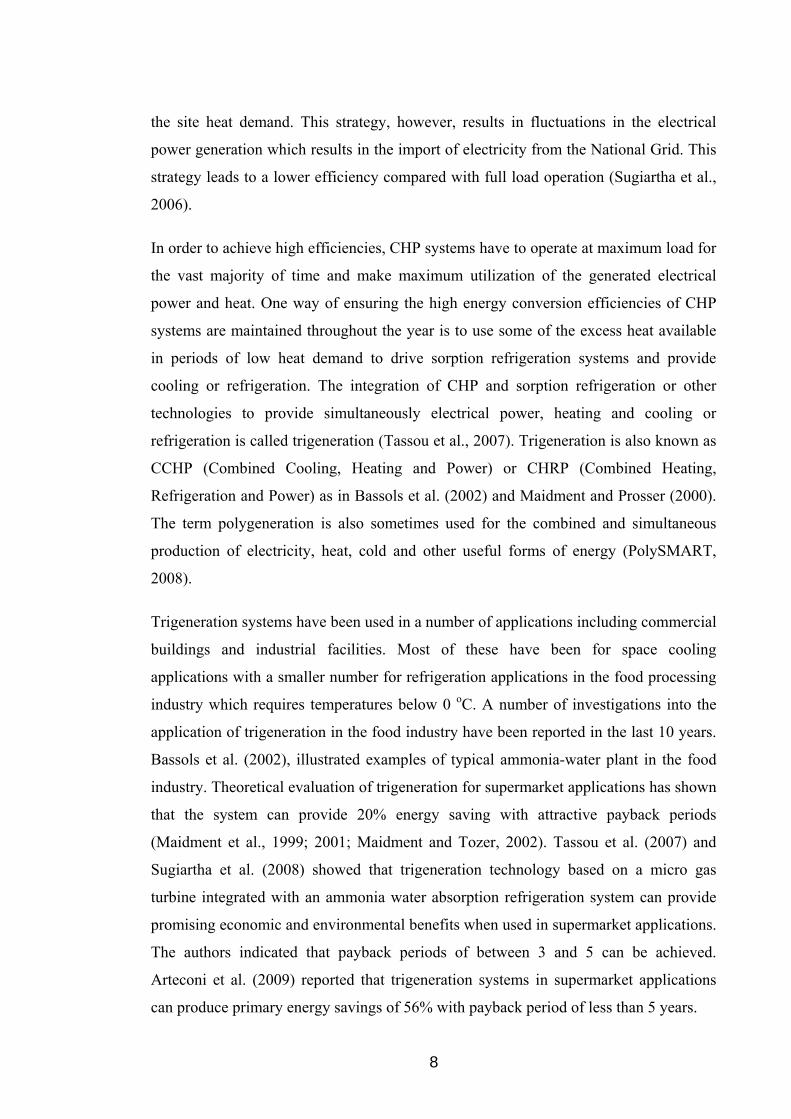
In order to achieve high efficiencies, CHP systems have to operate at maximum load for

the vast majority of time and make maximum utilization of the generated electrical

power and heat. One way of ensuring the high energy conversion efficiencies of CHP

systems are maintained throughout the year is to use some of the excess heat available

in periods of low heat demand to drive sorption refrigeration systems and provide

cooling or refrigeration. The integration of CHP and sorption refrigeration or other

technologies to provide simultaneously electrical power, heating and cooling or

refrigeration is called trigeneration (Tassou et al., 2007). Trigeneration is also known as

CCHP (Combined Cooling, Heating and Power) or CHRP (Combined Heating,

Refrigeration and Power) as in Bassols et al. (2002) and Maidment and Prosser (2000).

The term polygeneration is also sometimes used for the combined and simultaneous

production of electricity, heat, cold and other useful forms of energy (PolySMART,

2008).

Trigeneration systems have been used in a number of applications including commercial

buildings and industrial facilities. Most of these have been for space cooling

applications with a smaller number for refrigeration applications in the food processing

industry which requires temperatures below 0 oC. A number of investigations into the

application of trigeneration in the food industry have been reported in the last 10 years.

Bassols et al. (2002), illustrated examples of typical ammonia-water plant in the food

industry. Theoretical evaluation of trigeneration for supermarket applications has shown

that the system can provide 20% energy saving with attractive payback periods

(Maidment et al., 1999; 2001; Maidment and Tozer, 2002). Tassou et al. (2007) and

Sugiartha et al. (2008) showed that trigeneration technology based on a micro gas

turbine integrated with an ammonia water absorption refrigeration system can provide

promising economic and environmental benefits when used in supermarket applications.

The authors indicated that payback periods of between 3 and 5 can be achieved.

Arteconi et al. (2009) reported that trigeneration systems in supermarket applications

can produce primary energy savings of 56% with payback period of less than 5 years.

9

The economic viability of trigeneration for supermarket applications is very sensitive to

the price of grid electricity relative to the price of natural gas which is also known as

spark ratio. A gas powered trigeneration system will be economically attractive when

the spark ratio is greater than 3.3 (Tassou et al., 2007; Sugiartha et al., 2006; 2008). In

the UK, the recent increases in electricity and fuel prices have increased the spark ratio

and price gap between grid electricity and natural gas (spark gap) as shown in Figure

1.5. The good trend of spark ratio and spark gap together with increased concerns about

the environmental impacts of the retail food industry have increased interest in the

application of trigeneration technology to supermarkets in the UK.

As indicated earlier the main environmental impact of refrigeration systems are from

energy use and from refrigerant leakage. Alternative solutions to reduce the emissions

from refrigerant leakage are to use environmentally friendly refrigerants, such as natural

refrigerants or secondary refrigerants. Melinder and Granryd (2010) showed that

indirect refrigeration systems can reduce refrigerant charge drastically down to 5 - 15%

of that of traditional DX-systems.

Figure 1.5 Comparison of electricity and gas price in the UK (Source: Moorjani, 2009)

CO2 is natural refrigerant that has received considerable attention in the last 10 years.

Research and development particularly in Scandinavia, USA and Japan is aimed at

developing CO2 systems for a wide range of applications ranging from small

commercial refrigeration and air conditioning systems to car air conditioners and larger

commercial and industrial systems, including supermarkets. Most of the development

work on CO2 systems for supermarkets has taken place in Scandinavia and Germany.

0

2

4

6

8

10

12

0

2

4

6

8

10

12

0 1 2 3 4 5 6 7 8 9 10 11 12

Sp

ark

ga

p (

p/k

Wh

)

Sp

ark

ra

tio

Months (from Nov-2007 to Oct-2008)

Spark ratio

Spark gap

10

However significant interest in CO2 refrigeration has also been demonstrated in some

supermarkets in the UK, Australia, Canada and the Latin America.

In the UK, there is increasing interest by supermarket chains to move towards

sustainable and environmentally friendly refrigeration technologies including CO2

refrigeration. In 2009 there were 46 stores across the UK using CO2 based technology,

increasing from just 14 stores in 2008. Sainsbury’s is committed to phasing HCFCs and

HFCs and plans to switch to CO2 in all of its stores by 2030 with the first 135 stores set

to be converted by 2014. Tesco plans to introduce CO2 refrigeration in 150 stores by

2012. M&S and Morrisons converted 34 stores to CO2 by 2009 and Waitrose is

implementing an innovative system based on HC refrigerant (Walravens et al. 2009).

Most of the early systems operate on the subcritical cycle where CO2 is used in a

cascade arrangement with a conventional refrigeration system operating with ammonia,

HCs or HFCs. Such arrangements keep the pressures in the CO2 system relatively low,

but still suffer the disadvantage of using another refrigerant such as HFC with its

associated global warming implications.

Another way of improving the performance of CO2 refrigeration as well as totally

avoiding the use of HFC refrigerants is by using cascade CO2 refrigeration with HC or

ammonia refrigerant in the high stage system. Bellstedt (2008) indicated that CO2/NH3

systems can achieve yearly energy savings of up to 35% over conventional R-404A

systems. However, most retailers in the UK have been reluctant to use HC and ammonia

in supermarkets due to their flammability and toxicity. Another option is to use

absorption/adsorption refrigeration for the high stage in a cascade CO2 refrigeration

arrangement. This solution can be particularly advantageous when the sorption

refrigeration system is driven by waste heat or is integrated with a CHP system in a

trigeneration system arrangement.

11..44 RReesseeaarrcchh pprroojjeecctt ddeessccrriippttiioonn

Trigeneration can provide substantial improvement in the overall energy efficiency over

the conventional supermarket energy approach of separate provision of electrical power

and heat energy. Trigeneration can also make significant contributions to the reduction

of the environmental impacts of food factories and supermarkets. This research aims to

11

increase further the energy and CO2 emission savings potential of trigeneration through

its integration with CO2 refrigeration systems.

The experimental part of the research programme is based on a trigeneration system that

incorporates three main modules; CHP module, sorption refrigeration system module,

and a refrigeration load module. The approach employed is to use the exhaust gases of a

microturbine CHP unit to drive an ammonia-water absorption refrigeration system,

which cool a secondary fluid for refrigeration purposes. The heat transfer between the

microturbine exhaust heat exchanger and the generator of the absorption system is

performed by a heat transfer fluid in a closed heat transfer loop arrangement. A

schematic diagram of the trigeneration arrangement test facility using thermal oil as the

heat transfer medium between the microturbine and absorption refrigeration system is as

shown in Figure A-1 (Appendix-A). It can also be found in Tassou et al. (2008).

The CHP module is a Bowman 80 kWe recuperated microturbine generation package

MTG80RC-G with in-built boiler heat exchanger (exhaust heat recovery heat

exchanger). The microturbine consists of a single stage centrifugal compressor, single

radial turbine within an annular combustor and a permanent magnet rotor (alternator) all

on the same rotor shaft. Other systems in the engine bay include the fuel management

system and the lubrication/cooling system. Heat recovery from the exhaust gases is

performed in a stainless steel flue-gas/liquid heat exchanger. The heat recovery fluid is

Diphyl-THT high performance synthetic heat transfer fluid that can operate at

temperatures up to 340 oC.

The sorption refrigeration system employed is a packaged gas fired ROBUR ACF-60LB

chiller. The performance of the unit in its gas fired format was established from tests in

the laboratory. For brine flow temperatures between -11 oC and +3 oC, the refrigeration

capacity of the unit was found to vary from 8.5 kW to 15 kW and the COP from 0.32 to

0.57 (Tassou et al., 2008). The modified unit performed as well if not better than the gas

fired unit. At brine flow temperature of -8.0 oC both units had a refrigeration capacity of

12 kW and a COP of around 0.53. The optimum COP of the absorption chiller was

achieved at oil temperature of 195 oC (Suamir et al., 2009).

The use of secondary fluid such as propylene glycol, potassium-formate and sodium

chloride for supermarket applications is one disadvantage of the previous trigeneration

12

system. The high energy consumption of the secondary fluid pumps due to the high

viscosity and poor thermodynamic performance of available secondary fluids was the

main disadvantage of the previous trigeneration system. Another disadvantage of the

system was the relatively low COP of sorption refrigeration systems particularly when

they operate at low refrigeration temperatures. The system would be more applicable for

chilled food refrigeration applications. Thus a separated system would be required to

satisfy the frozen food refrigeration demand. The approach followed in this research to

overcome the disadvantages of the secondary single phase fluid system is to integrate

the trigeneration system with a CO2 refrigeration system. For medium temperature

applications the CO2 can be used as a volatile secondary fluid with the cooling produced

by the trigeneration system providing the heat rejection medium for the condensation of

CO2. For low temperature frozen food applications cooling from the trigeneration

system can be used for the condensation of CO2 which can be used as a primary

refrigerant in a low temperature vapour compression system.

The utilisation of CO2 as a secondary refrigerant can minimise the use of conventional

secondary fluids and increase further the energy savings potential of trigeneration

systems. The pressure drop and consequently the pump power required for the

secondary fluid through the distribution pipe-work and cooling coils in the display

cabinets is primarily a function of the viscosity of the secondary fluid. The viscosity of

liquid CO2 is much less than the viscosity of common secondary fluids and thus the

power that will be required to circulate CO2 from the trigeneration system to the display

cabinets will be very small compared to the power required for conventional secondary

refrigerants. It is therefore estimated that the energy savings for the integrated CO2 -

trigeneration system will be higher than the trigeneration system with conventional

secondary fluids. Other advantages of using CO2 as secondary refrigerant are excellent

heat transfer properties, good material compatibility and smaller pipe size requirements.

11..55 RReesseeaarrcchh oobbjjeeccttiivveess

The main objective of this research project is, to design, develop and evaluate proof of

concept integrated trigeneration and CO2 refrigeration systems for food refrigeration

applications. Such systems should combine the efficiency advantages of trigeneration

with the advantages of CO2 as a primary refrigerant in low temperature systems and as

13

secondary refrigerant in medium temperature systems. The project will also investigate

heat transfer phenomena of the evaporator coils to ensure maximum thermodynamic

performance for the CO2 system.

11..66 SSttrruuccttuurree ooff tthhee tthheessiiss

The thesis comprises of eight chapters. Chapter 1 provides an introduction of the work

in the thesis. Following the introduction in Chapter 1, Chapter 2 presents an overview of

CO2 as a refrigerant and describes the concept of subcritical and transcritical CO2

refrigeration systems. The chapter also outlines recent development and applications of

CO2 refrigeration system for food preservation in supermarkets.

Chapter 3 discusses the design and construction of the test facility implemented for the

experimental investigation of the integration of CO2 refrigeration and trigeneration

systems. Chapter 4 presents modelling and performance analyses of CO2 evaporator

coils which covers heat transfer, pressure drop as well as simulation of frost formation

and its effect on the heat transfer performance of the coils. The chapter also describes

the application of the models for design and simulation of finned tube flooded and

direct expansion coils using CO2 and R-404A as refrigerants.

Chapter 5 provides experimental test results for the medium and low temperature

refrigeration systems as well as the performance of the overall CO2 refrigeration system

as a whole. This chapter also describes temperature and frost performance of the CO2

display cabinets as well as the validation of the numerical models.

A case study approach of the integration of volatile-DX CO2 refrigeration and micro-

turbine based trigeneration systems in supermarket applications is discussed in Chapter

6. The chapter describes briefly the case study supermarket in respect of its energy

consumption and emphasises the energy as well as environmental performance of the

supermarket energy system. Alternative solutions of integrated trigeneration and CO2

refrigeration systems are presented in Chapter 7. Economic analyses of the energy

system alternatives are also provided in this chapter.

Finally, Chapter 8 concludes the research work and identifies further investigations and

development required to improve system performance and optimisation.

14

CChhaapptteerr 22

CCOO22 RREEFFRRIIGGEERRAATTIIOONN IINN SSUUPPEERRMMAARRKKEETTSS

The choice of refrigerants in commercial refrigeration systems has been undergoing a

rapid change. One approach gaining popularity is the use of natural refrigerants. Natural

refrigerants such as ammonia, hydrocarbons (HC) and CO2 which were known earlier

are now experiencing resurgence after the problems to the environment have been rising

due to the use of the non-natural refrigerants. Natural refrigerants are environmentally

benign. They have been demonstrated to be a complete solution to synthetic refrigerants

such as CFC, HCFC and HFC (Lorentzen, 1995; Riffat et al., 1997). The interest to use

natural refrigerants in commercial sector varies amongst countries. CO2 and HC are

more attractive especially in Europe and Japan. In Northern European countries all of

those natural refrigerants are used. Applications of natural refrigerants in commercial

refrigeration are also widespread in Asia, USA, Australia, Canada and other countries

can be expected to follow (TOC, 2006).

The use of natural refrigerants has been resurfacing since about the last two decades, but

to implement them in supermarket refrigeration systems is still facing some barriers.

“Safety and technology” is considered as the most important barrier followed by

regulation, training and availability of the components. Some countries are probably

still facing a variety of challenges such as policy and situation as regards the phase out

of ODP and GWP refrigerants (ATMOsphere, 2010).

With respect to the local safety, CO2 is an excellent alternative among the natural

refrigerants, especially in supermarket refrigeration applications. CO2 is in group A1 of

15

the safety classification which is neither flammable nor toxic (BS EN 378-1, 2008;

ASHRAE Standard 34, 2007). On the other hand, ammonia carries a B2 safety

classification which indicates that it has a high toxicity and also carries a medium

flammability risk. Ammonia may be used in supermarket refrigeration systems with

several challenges in order to achieve significant acceptance (Pearson, 2008).

Combining ammonia with either a cascade CO2 or a secondary fluid CO2 is one

opportunity to apply it in supermarket as highlighted by Hinde (2011). Such

refrigeration system has been implemented in France (Rivet, 2002) and in Australia

(Bellstedt, 2008). HC, which is in group A3 (high flammability), may also have some

constrains. Possible leakage of HC refrigerant to the occupied area has to be restricted

below its lower flammability limit. However, with currently available safety devices,

better system tightness, and advanced design strategy in minimising refrigerant charge

some supermarkets in the UK and Germany have also employed HC in their

refrigeration systems (Gartshore and Benton, 2010; Lidl, 2011).

22..11 CCOO22 aass rreeffrriiggeerraanntt

CO2 is a natural substance that has been used in the refrigeration industry since 1866.

After reaching peak use for comfort cooling in the 1920s, its use declined to almost zero

with the introduction of chlorofluorocarbon (CFC) refrigerants in the 1930s (Bellstedt et

al., 2002; Bodinus, 1999). The rapid decline of CFC systems since last decade of the

20th century has resulted in a remarkable increase in refrigeration research for new

alternative refrigerants. The research includes the use of old natural refrigerants

including CO2 and ammonia. Since that period, CO2 has returned as practicable options

for various refrigeration applications (Pearson, 2005).

CO2 (R-744) is an environmentally benign refrigerant. It has an ODP of zero and a very

low global warming potential (GWP) of 1. The main advantages of CO2 compared to

other natural refrigerants are that it is non-toxic and non-flammable, which often limits

the application of other natural refrigerants such as hydrocarbons and ammonia. CO2

also has attractive thermo-physical properties: low viscosity, high thermal conductivity,

high specific heat capacity and high vapour density. These lead to good heat transfer in

evaporators, condensers, and gas coolers, allowing selection of smaller equipment

compared to HFC refrigerants.

16

One distinguishing characteristic of CO2 is its phase change properties; the triple point

is relatively high at -56.6 oC (5.2 bara) and the critical temperature is 31 oC (73.8 bara)

which is considered to be relatively low (ASHRAE, 2010). This may limit the

application flexibility of CO2 refrigeration systems and the phase change properties

from solid, liquid, and vapour as illustrated in Figure 2.1 should be thoroughly

considered in any potential applications.

Figure 2.1 CO2 expansion and phase change (Adapted from: ASHRAE, 2010)

Comparative performance of CO2 and selected refrigerants for medium and low

temperature refrigeration applications with the same operating conditions are shown in

Table 2.1. The refrigeration effect of CO2 is higher than R-404A but lower than other

natural refrigerants. This directly influences the amount of refrigerant that needs to be

circulated in a refrigeration system. The table also shows that CO2 has the lowest

pressure ratio among the selected refrigerants which is about 5 to 30% lower for MT

system and 15 to 50% for LT system. Having a lower pressure ratio indicates that CO2

can give greater volumetric and isentropic efficiencies. Another advantage of CO2

refrigerant which can clearly be seen in the table is that it has a very small suction gas

specific volume about 3 to 30 times lower than the other refrigerants for the MT system

and even lower for the LT system. This means that a CO2 refrigeration system will need

smaller size compressors and require smaller suction pipe diameters for the same

operating conditions.

73.8

5.2

13.3

28.0

Solid

Supercritical

Liquid/vapour

Solid/vapour

Solid/liquid

Vapour

Enthalpy (kJ/kg)

-32oC

-8oC

Triple point -56.6oC

-78.4oC 1.0

Pre

ssu

re (

bar

a)

31oC

307.4 (kJ/kg)

Liquid

17

Table 2.1 Comparative refrigerant performance per kW for MT and LT refrigeration

Refrigerant Pevap Pcond Pressure ratio

Refrigeration effect

Refrigerant mass flow rate

Suction gas specific volume

(bara) (bara) (kJ/kg) x 10-3 (kg/s) x 10-3 (m3/kg)

MT refrigeration system application

R-22 3.8 11.3 3.0 170.1 5.9 62.6

R-404A 4.7 13.6 2.9 124.2 8.1 42.8

R-290 3.7 10.3 2.9 300.5 3.3 126.1

R-1270 4.6 12.5 2.7 306.4 3.3 105.4

R-717 3.2 11.0 3.5 1134.1 0.9 396.8

R-744 28.0 68.9 2.6 153.1 6.5 13.9

LT refrigeration system application

R-22 1.5 11.3 7.5 159.4 6.3 150.3

R-404A 1.9 13.6 7.0 110.1 9.1 101.3

R-290 1.5 10.3 6.6 271.7 3.7 285.4

R-1270 2.0 12.5 6.3 281.3 3.6 234.4

R-717 1.1 11.0 10.2 1100.1 0.9 1082.2

R-744 13.3 68.9 5.2 153.3 6.5 29.9

Operating conditions: Refrigeration capacity 1 kW, degree of superheat 5 K, no sub-cooling, evaporating temperatures of -8 and -32 oC for MT and LT refrigeration systems respectively and condensing temperature of 28 oC for both systems. (Derived using EES, 2010)

CO2 also shows a very favourable pressure drop performance compared to most other

refrigerants. To demonstrate the advantage of CO2 refrigerant with regards to pressure

drop, three different graphs has been plotted as shown in Figures 2.2 and 2.3. The

pressure drops data of CO2 and other selected refrigerants were derived using EES

programme for the same geometry, operating conditions and refrigeration load.

Figure 2.2 (a) shows the comparisons of saturated liquid pressure drop of other

refrigerants to the pressure drop of CO2. It can be seen that the liquid pressure drop of

the CO2 refrigerant is significantly smaller than R-404A specifically at lower saturation

temperatures but it is about 1.7 to 2.5 times higher than R-1270, R-290 and R-22.

Ammonia (R-717) gives the lowest saturated liquid pressure drop for given evaporating

temperature range. The acceptable saturated liquid pressure drop of the CO2 is,

however, 5 to 9 times greater than the other refrigerants. This shows that CO2 can

perform better compared to other selected refrigerants except ammonia in term of

saturated liquid pressure drop which also make it suitable for use as a secondary fluid.

The saturated vapour pressure drop ratios of other refrigerants to CO2 refrigerant are

presented in Figure 2.2 (b). CO2 has considerably lower vapour pressure drop than the

other refrigerants apart from ammonia. The figure also shows that the lower the

18

saturation temperature the more favourable the CO2 refrigerant compared to other

selected refrigerants in respect of saturated vapour pressure drop.

Figure 2.2 Liquid and gas pressure-drop ratio for selected refrigerants and CO2 at different

saturated temperatures, investigated at the same operating conditions (Obtained using EES, 2010)

Figure 2.3 describes the acceptable pressure drop of saturated liquid and gas line which

is equivalent to 1 K saturated temperature drop. For the same saturation temperature, the

acceptable pressure drop of CO2 is significantly higher than the other selected

refrigerants. CO2 can tolerate pressure drop of approximately 45 kPa for LT systems

and 80 kPa for MT applications. While the other refrigerants can accept pressure drop

as high as 5 kPa and 15 kPa for respectively LT and MT applications. The fact that

(b) Saturated vapour pressure-drop ratio (a) Saturated liquid pressure-drop ratio

(a)

0.0

0.2

0.4

0.6

0.8

1.0

1.2

1.4

1.6

1.8

2.0

-35 -30 -25 -20 -15 -10 -5 0 5 10 15

Saturation temperature (oC)

Liq

uid

pre

ssu

re d

rop

rat

ioR-404A R-717R-744 R-290R-1270 R-22

(b)

0

1

2

3

4

5

6

7

8

-35 -30 -25 -20 -15 -10 -5 0 5 10 15

Saturation temperature (oC)

Vap

ou

r p

ress

ure

dro

p r

atio R-404A R-717 R-744

R-290 R-1270 R-22

19

higher pressure drop can be tolerated with CO2 in the evaporator and suction line before

system performance is seriously affected, higher evaporating temperature can be

achieved and smaller pipe diameter can be used compared to other refrigerants.

Figure 2.3 Acceptable pressure drop for CO2 and selected refrigerants in gas and liquid lines of a refrigeration system (Obtained using EES, 2010)

The smaller components and pipe diameter that can be employed with CO2 lead to a

significant reduction in the refrigerant charge required for a given refrigeration load

compared to HCFC and HFC refrigerants. For centralised supermarket refrigeration

systems, refrigerant charge of CO2 is expected to be approximately 50% of that of

HCFC and HFC refrigerants. The specific

refrigerant charge of CO2 in supermarket

applications is in the range 1 to 2.5 kg/kW

as shown in Table K-1 (Appendix K). CO2

is also a relatively cheap refrigerant. Its

price is about 50% lower than that of

ammonia and approximately 6 to 9 times

lower compared to the price of HCFC,

HFC and HC refrigerants as can be seen in

Table 2.2.

As with all other refrigerants, the choice of lubricant is very important with CO2

refrigeration systems. The primary function of lubricants is to reduce friction and

Table 2.2 Price comparison of selected refrigerants

Refrigerants Price (£/kg) Price ratio

R-22 17.00 7.3

R-404A 13.20 5.7

R-290 19.25 8.3

R-1270 22.10 9.5

R-717 5.60 2.4

R-744 2.31 1.0

(Source: Dean & Wood, 2011)

0

20

40

60

80

100

120

140

-35 -30 -25 -20 -15 -10 -5 0 5 10 15

Saturation temperature (oC)

Acc

epta

ble

pre

ssu

re d

rop

(kP

a)

R404A R717 R744

R290 R1270 R22

20

minimise wear in the compressor. A lubricant achieves this by interposing an oil film

between sliding surfaces to reduce direct solid to solid contact and lower the coefficient

of friction. A compatible lubricant will be able to continuously keep the lubrication film

in the compressor. Lubricants being considered suitable for CO2 include mineral oils

(MO), poly alpha olefin (PAO) and hydro treated mineral oil. Polyol ester (POE) oil

which is commonly used for HFC refrigerants also has good miscibility with CO2

(Lommers, 2003).

In spite of the above advantages, CO2 also has some disadvantages. One main drawback

of CO2 as a refrigerant is its high working pressures compared to those of natural and

synthetic refrigerants. This means that for CO2 systems, components must be designed

to withstand the high pressures and to reduce the safety risk due to high pressure

particularly for systems with high refrigerant charge such as supermarket systems (IIR,

2000).

Since CO2 offers a much higher volumetric capacity, the problem of the higher working

pressure can be overcome by optimal design involving smaller and stronger

components. Moreover, modern material development, design techniques and

technology in manufacturing processes have dramatically reduced the risks associated

with the high pressure (Proklima, 2008). However, to reduce costs some components in

CO2 plant such as in indirect systems and low temperature of cascade systems are

usually designed for maximum operating pressure (MOP) of 40 to 46 bars. In practice,

the most common and easiest way to protect against high pressure is to release some of

the CO2 charge from the plant through relief valves when the pressure reaches a certain

set value. This temporarily reduces the pressure and temperature of CO2 in the system.

If the system remains at standstill, then the relief valves will repeatedly open and close

to keep the pressure low. In such cases, the plant can significantly lose the charge and

need to be recharged to compensate for the lost CO2. For a CO2 refrigeration system

which is designed for possibly long downtime, a small independent refrigeration unit

can be fitted to cool down the CO2 liquid to levels where saturated pressure is less than

the design pressure. Another technique is to employ a receiver which can withstand

pressures higher than the saturated pressure of CO2 at high ambient temperatures. In the

event of stoppage, the plant is pumped down and all CO2 charge is stored in the

21

receiver. For UK weather conditions (Met Office, 2009) a 75 bar design pressure for the

receiver is considered safe.

Another safety issue with CO2 refrigerant is the concentration level of CO2 gas in the

occupied area in the event of leakage. CO2 is heavier than air and tends to displace the

air from an occupied area close to the floor. CO2 is also odourless and cannot be

smelled by people. Leakage from the CO2 system could make the level of CO2

concentration too high which can risk health damage to the persons in the confined

space such as in the plant room. A similar risk exists with CFC, HCFC and HFC

refrigerants. In practice, this is considered to be a controlled risk which can be

prevented with proper leak detection and space ventilation. A reliable CO2 detector is

required to ensure the plant room is safe for people and to keep the concentration level

of CO2 in the range of good indoor air quality (human comfort) which should not

exceed 1000 ppm (ASHRAE Standard 62.1, 2007).

22..22 DDiiffffeerreenntt ttyyppeess ooff CCOO22 rreeffrriiggeerraattiioonn ssyysstteemmss

In supermarket applications three types of refrigeration systems are mainly employed

which include stand-alone (integral), condensing units and centralised supermarket

systems (IPCC, 2005). In centralised systems, a number of different design approaches

can be adopted that fall into two major categories: subcritical cascade systems and

transcritical systems. Subcritical cascade systems operate at moderate pressures and

employ two refrigerants one for refrigeration and another for heat rejection whereas

transcritical systems operate at high pressures at high ambient temperatures but employ

only CO2 as refrigerant.

2.2.1 Subcritical CO2 refrigeration systems

As discussed earlier, the CO2 refrigerant has a low critical point which limits the

maximum condensing temperature to around 25 oC (Rhiemeier et al., 2009). In order to

keep the cycle in the subcritical region all year round, it is necessary to use a cascade

system to absorb the heat rejected in the condenser of the low pressure system. A

schematic diagram of a simple cascade system using CO2 as the low stage cycle is

shown in Figure 2.4. The cascade system is constituted by two single stage systems

22

connected by a heat exchanger. The high pressure system which rejects heat to the

ambient or cooling medium can employ a variety of refrigerants.

Figure 2.4 Schematic diagram of a cascade arrangement using CO2 as the low stage cycle

The performance of subcritical cascade systems in supermarket applications has been

reported by a number of investigators (Campbell et al., 2006; Hinde et al., 2009). Other

investigations have also been conducted on the use of all natural refrigerants in cascade

arrangements. Fernandez-Seara et al. (2006) studied a compression–absorption cascade

refrigeration system using CO2 and ammonia as the refrigerants at the lower stage.

Sawalha et al. (2006) evaluated theoretically and experimentally the performance of an

ammonia/CO2 cascade refrigeration system for a supermarket application. The authors

have reported that the cascade arrangement could provide better COP compared to a

conventional R-404A system. Similar cascade ammonia/CO2 systems have also been

investigated by Lee et al. (2006); Getu and Bansal (2008); Bingming et al. (2009) and

Dopazo et al. (2009). Bansal and Jain (2007) reviewed cascade refrigeration systems

and analysed systems using CO2 in the low stage cycle, while the high stage employed a

variety of refrigerants including propane, propylene, ammonia and R-404A.

2.2.1.1 All-volatile systems

Figure 2.5 shows a simplified all-volatile subcritical CO2 system arrangement. With this

arrangement CO2 works as secondary fluid for both chilled and frozen food systems

Cascade HX

HT condenser

HT evaporator

CO2 condenser

CO2 evaporator

Refrigerated medium

Ambient or cooling medium

CO2 circuit

High stage circuit

Electrical power

Electrical power

Absorbed heat

Rejected heat

23

which are arranged as parallel units. The CO2 circuits are connected to primary

refrigeration systems which act as the high pressure stages of the arrangement. The

evaporating temperature of the high stage system must be lower than the saturation

temperature of the corresponding secondary loop system. The temperature difference

depends on the effectiveness of the cascade condenser. At the same time, the saturation

temperatures of the secondary loops should be low enough to keep the chilled food in

the range between -1 oC to +4 oC and frozen food from between -15 oC and -18 oC.

Supermarkets commonly use saturation temperatures in the range between -30 oC and -

35 oC for the LT loop and from -7 oC to -10 oC for the MT loop. With the pressures

corresponding to these temperatures, it is possible to use conventional refrigeration

pipes and components to handle CO2.

Figure 2.5 Parallel MT and LT indirect system with CO2 as secondary fluid

The CO2 circuit contains a receiver that the CO2 returning from the cascade condenser.

The receiver also functions as a liquid reservoir for the CO2 pump. The level of liquid in

the receiver can be connected to the pump controller to ensure the pump works at an

acceptable net positive suction head (NPSH). The size of the receiver should, therefore,

be carefully designed to be able to accommodate the fluctuations of the liquid CO2

caused by variation in the load.

The pump circulates the liquid CO2 in the secondary loop from the receiver to the

evaporator and keeps the evaporator wet (flooded) for all load conditions. In the

evaporator, liquid CO2 absorbs heat and some of it evaporates. The saturated mixture

then flows to the cascade condenser where it rejects heat to the high stage system and

MT cabinet

High stage system

Condenser (a)

Cascade condenser

MT CO2 secondary loop

LT cabinet

High stage system

Condenser (b)

Cascade condenser

LT CO2 secondary loop

24

becomes liquid again. From the condenser the CO2 returns back to the receiver for the

repetition of the cycle.

Figure 2.6 All-volatile CO2 subcritical system with LT DX circuit; (a) cascade arrangement with vapour compression cycle on HT section, (b) alternative arrangement for HT system with sorption chiller, (c) Other arrangement for cascade joint

Another arrangement for all-volatile subcritical CO2 system is shown in Figure 2.6. The

system employs an LT DX circuit and LT secondary loop for the low temperature

system. The arrangement uses only one high stage system which can minimise the

refrigerant charge and safety risk if other natural refrigerants such as HC and ammonia

are used. The liquid CO2 from the MT receiver is distributed to both the MT secondary

loop and the LT system. For the LT system the liquid CO2 flows through a valve (ICM)

where it is expanded to the low stage evaporating pressure. The ICM valve is

modulated to maintain the temperature and liquid level of the LT secondary loop

relatively constant. From the ICM valve the two phase mixture enters the LT receiver

where it is separated into two phases. The liquid phase flows through the LT secondary

loop and the saturated gas enters the LT compressor and is compressed to the MT

pressure level. The hot gas from the LT compressor then mixes with the two phase

mixture. The mixture then enters the cascade condenser and returns back to the MT

receiver to complete the cycle. An internal heat exchanger (IHX) might be required

between the suction line of the LT compressor and the liquid line upstream of the ICM

valve to ensure there is no liquid at suction line of the compressor.

(b)

Sorption chiller

(c)

MT cabinet

LT compressor

LT cabinet

High stage system

Condenser(a)

Cascade condenser

ICM

25

The above arrangement can also employ a sorption chiller on the high stage as an

alternative solution to a vapour compression system as shown in Figure 2.6 (b),

particularly where there is waste heat available, as is the case with local power

generation to drive the sorption chiller. Different arrangement for the CO2 cascade

coupling can also be applied as can be seen in Figure 2.6 (c).

The volatile subcritical CO2 solutions are relatively simple systems to implement and

offer advantages over conventional water based brine systems. They require

considerably smaller pipes and components, and installation cost savings can reach

12% (Danfoss, 2010). With respect to energy consumption, the author stated that the

secondary CO2 solutions can be more energy efficient by about 30% for the LT system

and 20% for the MT system. Rogstam (2010) reported that the secondary CO2 could

provide energy reduction for pumping of the order of 90% compared to fixed speed

brine pumps and 50% reduction compared to variable speed brine pumps. Another

possibility is to operate the CO2 system on gravity circulation.

2.2.1.2 Volatile-DX system

A volatile-DX system is a subcritical CO2 system with MT secondary loop cascaded

with a LT DX circuit as shown in Figure 2.7. The advantage of this system is that it is a

simple system without LT pump or LT receiver for the LT circuit.

Figure 2.7 Cascade CO2 refrigeration with MT secondary loop and LT DX system; (b) Alternative cascade coupling arrangement for HT system, (c) Alternative LT evaporator arrangement. (Adapted from: Sawalha et al., 2006)

(c)

From MT liquid receiver

To LT compressor

(b)

LT system

HT system

MT system

LT cabinet

MT cabinet

LT compressor

High stage system

Condenser

(a)

Cascade condenser

EXV

26

Subcritical CO2 system solutions in supermarket applications provide several

advantages over conventional systems. The HFC refrigerant charge on the high stage

system can be significantly reduced which reduces impact on the environment. The high

stage system can be located in a secured machine room with no public access. This

gives possibility to employ other natural refrigerants such as ammonia and

hydrocarbons with minimum safety risk. It has also been reported that the energy

consumption of subcritical CO2 supermarket solutions can be comparable to that of

R-404A DX systems (Sawalha et al., 2006; Hinde et al., 2009; Rhiemeier et al., 2009).

To date many subcritical CO2 systems have been implemented in EU countries such as

Denmark, Germany, Norway, Sweden, Italy and the UK (Rhiemeier et al., 2009). Such

systems have also been reported in supermarket applications in Australia, Canada and

the Latin America as reported (Bellstedt, 2008; CanmetENERGY, 2009; Verdemar,

2010).

2.2.2 All-CO2 systems

All-CO2 systems employ CO2 as the only working fluid without the need of a second

refrigerant on the high pressure side of a cascade arrangement for heat rejection. This

minimises the environmental impact from the refrigerant leakage but requires the

system to operate above the critical temperature of CO2 (transcritically) at high ambient

temperatures. At temperatures above the critical point, heat rejection occurs whilst CO2

in the gaseous state and takes place in a gas cooler. This necessitates high pressures

which can lead to high power consumption. Therefore, the pressure of the gas cooler

becomes very important operating parameters which need to be controlled in order to

obtain best performance.

In transcritical stage the operating pressure of the gas cooler becomes independent of

the gas cooler exit temperature. Figure 2.8 shows that different operating pressures can

be selected at a particular gas cooler exit temperature. The figure also illustrates

optimum operating pressures at different exit temperatures of the gas cooler.

The temperature of CO2 exits the gas cooler depends on the ambient temperatures and

the heat rejected from the gas cooler. The exit temperatures can be maintained close to

the ambient temperatures by modulating the speed of the cooling fans. The pressure of

27

the gas cooler is regulated by a high pressure expansion device (ICMT valve) and the

optimum operating pressure can be achieved by modulating the ICMT valve which

incorporates a proportional integral differential (PID) controller. Control parameters of

this controller include the exit temperature and the actual pressure of the gas cooler.

Figure 2.8 COP of a CO2 transcritical cycle vs. pressures of the gas cooler at different exit gas temperatures (T1) (Source: Sawalha, 2008)

2.2.2.1 Parallel CO2 system arrangement

Figure 2.9 illustrates a parallel CO2 system which constitutes two separate DX circuits.

One circuit is for chilled food (MT) display cabinets and another for frozen food (LT)

cabinets. The MT system uses single stage compression whereas two-stage compression

with intercooler is normally used for the LT system. In practice, both systems normally

use multi-compressor packs. Internal heat exchangers (IHX) are also commonly

employed to ensure the systems have superheated CO2 vapour at the suction line of the

compressors.

The use of two-stage compression with intercooler can reduce the pressure ratio and

discharge temperature of the LT compressors. The intercooler de-superheats the CO2

vapour before the second stage of compression. This can keep the discharge temperature

of the LT CO2 system below 140 oC which is considered as an acceptable value for the

CO2 compressors (Girotto et al., 2004). The two stage compression can also improve

volumetric and isentropic efficiencies of the LT compressors.

Gas cooler pressure (bar)

Optimum pressure

75 90 105 120 135

2.5 2.0 1.5 1.0 0.5 0.0

CO

P

28

Figure 2.9 Simplified parallel CO2 refrigeration systems

2.2.2.2 Integrated CO2 system solutions

In the integrated system solutions, both MT and LT circuits are connected to the same

heat rejection circuit. The arrangement of the three circuits depends on the system

solutions chosen. These are described in the following sections.

Transcritical CO2 booster system

A simplified diagram of a transcritical CO2 booster system is shown in Figure 2.10. The

system is divided into 4 pressure levels. The high pressure is in the range between 60

and 90 bara. It incorporates the discharge of HT compressor, gas cooler and high

pressure expansion device (ICMT). The intermediate pressure is from 30 to 40 bara.

This section begins from downstream the ICMT valve incorporates the liquid receiver

and the bypass valve (ETS) and ends at the expansion valves of the MT and LT circuits.

The medium pressure level ranges from 26 to 29 bara and includes the discharge of the

LT compressor, the MT evaporator and suction of the HT compressor. The low pressure

section in the pressure range from 12 to 14 bara incorporates the LT evaporator and

suction line to the LT compressor.

The main function of the bypass valve (ETS) is to keep the pressure in the intermediate

pressure section relatively constant by bypassing saturated gas from the receiver to the

medium pressure section. The bypass valve also ensures a differential pressure exists

LT display cabinet

Liquid receiver

IHX

Gas cooler

(b) LT system

Inter cooler

ICMT

EXV

MT display cabinet

Gas cooler

Liquid receiver

(a) MT system

EXVICMT

IHX

29

between the liquid line after the liquid receiver and the MT evaporator coils for the

proper operation of the MT expansion valve.

Figure 2.10 All-CO2 booster system with gas bypass (Adapted from: Danfoss, 2008a)

In a CO2 booster system, the lower the intermediate pressure the better it is for system

efficiency which can be explained as follows: The intermediate pressure does not

influence the pressure ratio of the LT and HT compressors which means the power

consumption of the compressors remains constant. The refrigeration effect of the MT

and LT evaporators, however, will increase when the intermediate pressure reduces.

This will improve the refrigeration capacity of the systems which leads to a higher

system efficiency.

Figure 2.11 All-CO2 booster system installed in the Refrigeration Laboratory, Brunel University

MT cabinet LT cabinet

ETS

ICMT IHX

Liquid receiver

LT compressor

HT compressors

Gas cooler

EXV

EXV

High pressure

Medium pressure

Intermediate pressure

Low pressure

LT compressor

HT compressors

ICMT

Gas bypass valve

30

For the operation of the MT expansion valve, at least a 4 bar pressure difference is

maintained over the MT evaporator pressure (Danfoss, 2008a). Other factors that

influence the operation of the bypass valve and control of the intermediate pressure

include the gas cooler exit pressure and temperature and the requirement to have

superheated CO2 vapour at the entry to the HT compressor.

Figure 2.11 shows a small size plant with integrated all-CO2 booster system. The CO2

system employs an air cooled gas cooler, two parallel compressors for the high pressure

system and a single compressor for the low pressure cycle. ICMT and ICM valves are

utilised for the high pressure expansion device and the gas bypass valve respectively.

The CO2 plant incorporates a Danfoss controller for the system control and monitoring.

Cascade CO2 system with flash gas bypass

A cascade CO2 system with flash gas bypass is shown in Figure 2.12. The high stage or

heat rejection section is similar to the booster system. The difference is that the LT

system is cascaded as an individual circuit with the HT system for heat rejection. The

MT evaporators are divided into two groups: one provides refrigeration to the MT

display cabinets and the other condenses the CO2 gas for the LT systems.

Figure 2.12 Integrated cascade all-CO2 system with flash gas bypass

This solution has been implemented in a number of UK supermarkets (Campbell, 2009).

Performance investigations have shown its seasonal energy performance to be about the

MT display cabinets

LT pack

LT displaycabinets

HT pack LT condenser

Gas cooler

HT liquid receiver

LT liquid receiver

Two LT condensers are cascaded to other HT packs

IHX

EXV

EXV

EXVICMT

ICM

31

same as that of conventional R-404A systems (Suamir and Tassou, 2010). In order to

gain full advantage of subcritical operation when the ambient temperature is low a

bypass valve is required in parallel with the ICMT valve (the bypass valve is not shown

in the diagram). The bypass valve closes when the ambient temperature is above a

certain value (the switching point between subcritical and transcritical operation) to

allow the ICMT valve to regulate the flow of CO2 gas out from the gas cooler and opens

below the switching point to allow the liquid CO2 to freely flow from the condenser

(gas cooler) to the liquid receiver.

Cascade CO2 system with a suction receiver

The cascade CO2 system with low pressure receiver is an improvement on the cascade

system with flash gas bypass. As can be seen in Figure 2.13, a suction receiver is added

on the high temperature side of the system. A back pressure valve is used instead of

bypass valve to minimise the fluctuation in the intermediate pressure due to pressure

and temperature variations at the outlet of the gas cooler.

Figure 2.13 Integrated cascade all-CO2 system with suction receiver

With this arrangement the MT evaporators can be set at zero superheat which can

increase the refrigeration capacity and the COP of the system. To ensure no liquid

enters the compressors, the system is equipped with oil cooler HX at the suction line of

ICMT

HT Pack

HT Receiver

Gas cooler

Suction receiver

MT display cabinets

LT pack

LT displaycabinets

LT condensers

LT liquid receiver

Two LT condensers are cascaded to other

HT packs

IHX

EXV

EXV

EXVBack pressure valve

Oil cooler HX

32

each HT compressor. According to Campbell (2009) this system is adaptable to variable

load; is less sensitive to charge and is easy to service.

Figure 2.14 presents an integrated cascade all-CO2 system with suction receiver

implemented in a UK supermarket. The store has sales area of 2,300 m2. The CO2

refrigeration plant of this store constitutes 4 HT packs and 2 LT packs. Every single HT

pack comprises 3 compressors, an air cooled gas cooler and a suction receiver (0.26 m3

volume). The LT pack incorporates 3 LT compressors, a liquid receiver (0.13 m3

volume) and 3 condensers. For reliability of the LT refrigeration system, each LT pack

is cascaded to three different HT packs as shown in Figure 2.13.

Figure 2.14 Integrated cascade all-CO2 plant in Tesco Ramsey, UK

22..33 SSuummmmaarryy

This chapter outlines advantages and disadvantages of the CO2 as a natural refrigerant.

The CO2 refrigerant, with ODP of zero and GWP of one, has lower impact to the

environment compared to HCFC and HFC refrigerants. Having attractive thermo-

physical properties, the CO2 refrigerant can provide good heat transfer in heat

exchangers of a refrigeration system which allows selection of smaller equipment than

HCFC and HFC refrigerants. The CO2 refrigerant is also non-toxic and non-flammable

which make it more advantageous than other natural refrigerants such as ammonia and

hydrocarbons. Moreover, the CO2 refrigerant is relatively cheap.

LT-pack of 20 kW refrigeration duty

HT pack of 40 kW refrigeration duty

33

The main downside of the CO2 refrigerant is its high working pressures. The problem of

the higher working pressure, however, can be overcome by using smaller and stronger

components. Some practical techniques to protect a CO2 refrigeration system against

high pressure are also explained in this chapter.

The chapter also describes different solutions and arrangements of the CO2 refrigeration

systems for supermarket applications which fall into two major categories: subcritical

cascade systems and transcritical systems. Subcritical cascade systems operate at

moderate pressures and employ two refrigerants one for refrigeration and another for

heat rejection whereas transcritical systems operate at high pressures at high ambient

temperatures but employ only CO2 as refrigerant. Recent developments of the CO2

refrigeration systems and their applications in supermarkets are also presented.

The following chapter will explain the design and the construction of the test facility

and will include the integration arrangement, system design and modelling, component

calculations, the components used, refrigeration load system and the test chamber.

34

CChhaapptteerr 33

DDEESSIIGGNN AANNDD CCOONNSSTTRRUUCCTTIIOONN OOFF TTHHEE TTEESSTT FFAACCIILLIITTYY

A small size CO2 refrigeration system for low and medium temperature applications

was designed and constructed to enable it to be integrated with the existing trigeneration

system to form an overall test facility. Instrumentation and monitoring systems were

also fitted to comprehensively monitor the performance of the system for evaluation

purposes.

For design purposes, mathematical models were established in the Engineering

Equation Solver (EES) platform which include pipe sizing, liquid receiver, evaporator-

coil models and system integration. The EES models were used to determine the

dimensions and capacity of the components. The models were also used to estimate the

performance of the integrated system at different operating conditions. Based on the

dimensions of the components a 3D drawing of the system was drawn using AutoCAD.

The CO2 refrigeration plant and the integration circuit were constructed in the

Refrigeration Laboratory of Brunel University. Technical drawings were produced

which include piping, instrumentation diagrams, liquid receiver, evaporator coils and

electrical control systems.

This chapter presents the mathematical models produced for the design of the CO2

refrigeration system. The evaporator coil models will be presented separately in

Chapter 4. This chapter also details the construction of the test facility which

35

incorporates mechanical, electrical, control and monitoring systems. The loading

systems and the environmental test chamber are also briefly described.

33..11 IInntteeggrraattiioonn aarrrraannggeemmeenntt

The test facility consists of three main modules; CHP module, absorption refrigeration

system module, and a refrigeration load module as described in Section 1.4. The main

construction is very similar to the previous trigeneration test facility (see Figure A-1 in

the Appendix A). The difference is only on the refrigeration load module. A subcritical

CO2 refrigeration system with chilled and frozen food display cabinets was used to

replace the water based secondary loop medium temperature display cabinet.

Figure 3.1 Integration arrangement of CO2 refrigeration and trigeneration systems

Figure 3.1 shows a schematic diagram of the integration arrangement of the CO2

refrigeration and trigeneration systems. The arrangement employs a water based

secondary loop which bridges the CO2 refrigeration system to the absorption chiller of

the trigeneration facility. Main components of the secondary loop include cascade

condenser, brine pump and evaporator of the absorption chiller. The CO2 refrigeration

system rejects heat to the secondary loop in the cascade condenser which is a brine/CO2

heat exchanger. The rejected heat is then released to the atmosphere from the condenser

of the absorption chiller which is driven by recovered heat from the CHP system.

CHP Plant MT load LT load

Absorption chiller

Exhaustgas

Air

Fuel

Electricity

Boiler HX

Generator Set

HTF pump

CO2 Refrigeration section

Cascade condenser

Water-based secondary loop

brine pump

36

33..22 MMaatthheemmaattiiccaall mmooddeellss

3.2.1 Integration model

The integration model uses the ambient conditions and required product temperature as

boundary conditions. The temperature for the products was assumed to be -1 oC to 5 oC

for medium temperature (MT) system and -15 oC to -18 oC for the low temperature (LT)

system. Evaporating temperatures for the medium and low temperature systems were

assumed to be -8 oC and -32 oC respectively. London weather data was assumed for the

purposes of heat rejection.

The integration model involved all components which influenced the performance of

the system and each component was treated as a single control volume. Mass and

energy balance principles were applied to the control volumes which can be expressed

as follows:

in out

skgmm

..

/ (3.1)

kWHmHmWQoutin

0....

(3.2)

3.2.1.1 Trigeneration system model

Figure 3.2 shows the schematic diagram of the CHP module. It can be seen that the fuel

energy of the CHP is used to generate electrical power and to produce heat. Some of the

heat is recovered in the gas/liquid heat exchanger (boiler HX) and the rest is released to

the atmosphere as waste heat. The boiler HX is circuited to the heat transfer fluid (HTF)

loop through which the useful heat is utilised to drive the absorption chiller.

The energy balance of the CHP model consists of fuel energy, useful energy (electrical

power and useful heat) and energy losses (waste heat and other losses). This energy

balance equation using CHP efficiency (ηCHP) can be expressed as:

CHPhCHPeCHPfCHP QWE ,,, (3.3)

The useful heat of the CHP can be determined from:

abshhCHPh QQQ ,, (3.4)

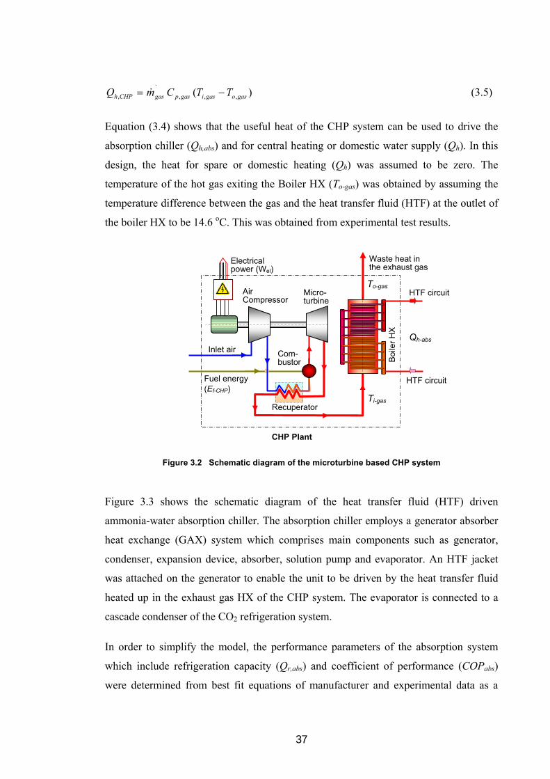
37

)( ,,,

.

, gasogasigaspgasCHPh TTCmQ (3.5)

Equation (3.4) shows that the useful heat of the CHP system can be used to drive the

absorption chiller (Qh,abs) and for central heating or domestic water supply (Qh). In this

design, the heat for spare or domestic heating (Qh) was assumed to be zero. The

temperature of the hot gas exiting the Boiler HX (To-gas) was obtained by assuming the

temperature difference between the gas and the heat transfer fluid (HTF) at the outlet of

the boiler HX to be 14.6 oC. This was obtained from experimental test results.

Figure 3.2 Schematic diagram of the microturbine based CHP system

Figure 3.3 shows the schematic diagram of the heat transfer fluid (HTF) driven

ammonia-water absorption chiller. The absorption chiller employs a generator absorber

heat exchange (GAX) system which comprises main components such as generator,

condenser, expansion device, absorber, solution pump and evaporator. An HTF jacket

was attached on the generator to enable the unit to be driven by the heat transfer fluid

heated up in the exhaust gas HX of the CHP system. The evaporator is connected to a

cascade condenser of the CO2 refrigeration system.

In order to simplify the model, the performance parameters of the absorption system

which include refrigeration capacity (Qr,abs) and coefficient of performance (COPabs)

were determined from best fit equations of manufacturer and experimental data as a

Waste heat in the exhaust gas

CHP Plant

Electrical power (Wel)

Inlet air

Fuel energy(Ef-CHP)

Recuperator

Air Compressor

Micro-turbine

Com-bustor B

oile

r H

X

Qh-abs

HTF circuit

HTF circuit

Ti-gas

To-gas

38

function of delivery brine temperature and ambient temperature. The equations are

given below:

Qr,abs = A0 + A1To + A2To2 + A3To

3 + A4To4 + A5To

5 + A6To6 + B1Tamb + B2Tamb

2 +

B3Tamb3 + B4Tamb

4 + B5Tamb5 + B6Tamb

6 (3.6)

COPabs = C0 + C1To + C2To2 + C3To

3 + C4To4 + C5To

5 + C6To6 + D1Tamb + D2Tamb

2 +

D3Tamb3 + D4Tamb

4 + D5Tamb5 + D6Tamb

6 (3.7)

Qr,abs is the refrigeration capacity of the absorption system (kW); To and Tamb are

delivery brine and ambient temperatures (oC) respectively. Constants of the equations

are listed in Table 3.1.

Table 3.1 Constants of the best fit equations

Parameter order

0 1 2 3 4 5 6

A 0.4962 -0.175 -0.06885 -0.01365 -0.001457 -0.000078 -0.0000016

B 0.00029 -0.00021 -2.492x10-8 1.337x10-6 -3.264x10-8 7.881x10-11

C 3.429 -9.55 -4.022 -0.8278 -0.08856 -0.004712 -0.0000985

D 0.008248 -0.004558 0.00000828 0.0000275 -7.190x10-7 2.076x10-9

The coefficient of correlations for the refrigeration capacity RQ2 = 0.9890 and the coefficient of performance

RCOP2 = 0.9974

Figure 3.3 Schematic diagram of the ammonia-water absorption chiller

In this model, Qr,abs was used as a boundary condition in simulating the integrated

system. The heat rejected from cascade condenser of the CO2 refrigeration system

(Qcond) should be smaller than Qr,abs. The results of the simulations are considered

invalid if Qcond is higher than Qr,abs.

RectifierIHX

Abs

orbe

r C

onde

nser

HTF jacket

Connections to the CO2 system

Connections to the Boiler HX CHP

Gen

erat

or

Evaporator

Expansion device

Qh-abs

Ti-htf To-htf

39

The heat required to drive the generator of the absorption system (Qh,abs) can be

calculated from:

absh

condabs Q

QCOP

,

(3.8)

The mass flow rate of the heat transfer fluid and power consumption of the HTF pump

can be determined from:

)( ,,, htfihtfohtfhtfabsh TTCpmQ (3.9)

pumphtf

htfihtfohtfhtfpumphtf

PPvmW

,

,,,

(3.10)

Ti-htf is the temperature of the HTF entering the generator jacket which has been found

from the experimental tests to be in the range between 190 and 200 oC. To,htf can be

determined by assuming the temperature difference of HTF across the generator to be

6 oC. (Po - Pi) and (ηhtf,pump) are the pressure losses in the HTF circuit and the total

efficiency of the HTF-pump. These were determined from tests to be 400 kPa and 0.45

respectively. The properties of the HTF can be determined from equations (B.1) to (B.4)

in Appendix B.

3.2.1.2 CO2 refrigeration model

The CO2 refrigeration system of the test facility is a volatile-DX system. The basic

principle of such system is explained in Section 2.2.1.2.

A simplified diagram of the CO2 system is shown in Figure 3.4. The system comprises

an LT CO2 compressor, LT and MT evaporators, a CO2 pump, expansion valve (EXV),

regulator valve (RV), liquid receiver, internal heat exchanger (IHX) and a cascade

condenser. The condenser is a CO2/brine HX. To provide flexibility to investigate

different arrangements for the LT compressor, the discharge line is split into two

branches. One branch is connected to the saturated gas line from the liquid receiver and

the other feeds directly into the liquid receiver. The figure also shows a bypass circuit

from the CO2 pump to the liquid receiver which allows the flow of CO2 refrigerant to

the MT evaporator to be varied to enable investigation of the effect of circulation ratio

(CR) on the performance of the MT evaporator.

40

Figure 3.4 Centralised volatile-DX CO2 section

The refrigeration cycle of the system is shown in Figure 3.5. The cycle refers to the

schematic diagram in Figure 3.4. It can be seen that the thermodynamic cycle of the

system consists of compression of a low pressure, low temperature superheated CO2

vapour to medium pressure level, followed by mixing of the superheated gas from the

compression process with saturated CO2 gas from the liquid receiver. The CO2 gas is

de-superheated and condensed in the cascade condenser and exits as saturated liquid.

Some of the liquid is pumped to the MT evaporator where evaporation takes place by

absorbing heat from air circulating in a refrigerated display cabinet. The CO2 exiting the

MT evaporator is a mixture of vapour and liquid. Liquid from the receiver flows

through an internal heat exchanger (IHX) before is expanded isenthalpically in the

expansion device (EXV) which results in a low temperature vapour-liquid mixture

entering the low temperature evaporator. The low temperature two phase mixture

evaporates in the LT evaporator removing heat from the LT refrigerated cabinet. The

vapour exiting the LT evaporator is superheated in the IHX and then compressed in the

LT compressor to complete the cycle.

To simulate the volatile-DX CO2 refrigeration system, some assumptions were made as

follows: steady state flow conditions; negligible thermal losses to the environment;

negligible refrigerant pressure drops in the pipes; degree of superheat of the LT

evaporator 5 K; CO2 leaving the condenser in saturated liquid; vapour quality at the exit

of MT evaporator to be 0.8 (it can be varied depending on the circulation ratio);

isenthalpic expansion in the EXV; negligible refrigerant pressure drop across the

MT Evaporator

LT Evaporator

IHXCO2 Compressor

CO2 Pump

EXV

RV

Liquid receiver

To the trigeneration system

1

2

3

11

10

9

5

4

6 7

8

12

Bypass circuit

Cascade condenser

33

35

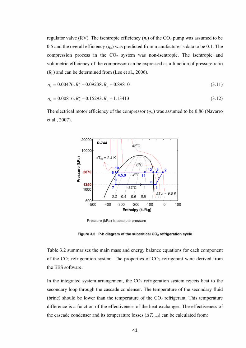
41

regulator valve (RV). The isentropic efficiency (ηs) of the CO2 pump was assumed to be

0.5 and the overall efficiency (ηo) was predicted from manufacturer’s data to be 0.1. The

compression process in the CO2 system was non-isentropic. The isentropic and

volumetric efficiency of the compressor can be expressed as a function of pressure ratio

(Rp) and can be determined from (Lee et al., 2006).

.2 89810.0.09238.0.00476.0 pps RR (3.11)

.2 13413.1.15293.0.00816.0 ppv RR (3.12)

The electrical motor efficiency of the compressor (ηm) was assumed to be 0.86 (Navarro

et al., 2007).

Figure 3.5 P-h diagram of the subcritical CO2 refrigeration cycle

Table 3.2 summarises the main mass and energy balance equations for each component

of the CO2 refrigeration system. The properties of CO2 refrigerant were derived from

the EES software.

In the integrated system arrangement, the CO2 refrigeration system rejects heat to the

secondary loop through the cascade condenser. The temperature of the secondary fluid

(brine) should be lower than the temperature of the CO2 refrigerant. This temperature

difference is a function of the effectiveness of the heat exchanger. The effectiveness of

the cascade condenser and its temperature losses (ΔTcond) can be calculated from:

Pressure (kPa) is absolute pressure

Enthalpy (kJ/kg)

-32oC

-8oC

8oC

Pre

ssu

re (

kPa

)

0.2 0.4 0.6 0.8

64,5,9

10

11

12 3 2

1

8

7

-500 -400 -300 -200 -100 0 100 500

1000

10000

20000

42oCR-744

2870

1350

∆Tsc = 2.4 K

∆Tsh = 9.8 K

42

353

43

TT

TTcond

(3.13)

354 TTTcond (3.14)

The position of each measurement point is shown in Figure 3.4. T3 and T4 are

temperatures of CO2 refrigerant entering and leaving the condenser respectively; T35 is

the temperature of brine entering the condenser.

Table 3.2 Equations for the CO2 refrigeration system (Numbers of the parameters refer to Figure 3.4)

Components Mass balance Energy balance

LT Compressor 21 mm

22.11 HmWHm scomp

s

sscomp

HHmW

12

1.

mvs

scomp

HHmW

..12

1

Mixing point 1223 mmm 12122233 HmHmHm

Condenser 43 mm condQHmHm 4433

Expansion valve (EXV)

76 mm

76 HH

LT Evaporator 87 mm 8877 HmQHm LT

Internal heat exchanger (IHX) 81 mm

65 mm 66118855 HmHmHmHm

655 HHmQIHX

CO2 pump

109 mm *

ospumpCO

PPvmW

91099

,2

MT evaporator 1110 mm 11111010 HmQHm MT

* For simulation purposes mass flow rate of the bypass line was assumed to be 0 kg/s.

The performance of the CO2 refrigeration system can be determined from:

comp

LTLT W

QCOP (3.15)

pumpCO

MTMT W

QCOP

,2

(3.16)

43

comppumpCO

LTMToverallCO WW

QQCOP

,2

,2 (3.17)

The coefficient of performance (COP) of the integrated system can be calculated from:

int,int WQ

QQCOP

absh

LTMT

(3.18)

Wint is the electrical power consumption of the various components of the integrated

system which can be expressed as:

pumpbrinepumphtfabspumpCOcomp WWWWWW ,,,2int (3.19)

Equation (3.19) shows that the integrated system consumes electricity for the LT CO2

compressor (Wcomp), CO2 pump (WCO2,pump), absorption chiller (Wabs), heat transfer fluid

pump (Whtf,pump) and brine pump (Wbrine,pump).

The electrical power of the brine pump can be determined from:

pumpbrine

brineibrineobrinebrinepumpbrine

PPvmW

,

,,,

..

(3.20)

(Po,brine-Pi,brine) and (ηbrine,pump) are pressure head and total efficiency of the brine pump

which were assumed to be 250 kPa and 0.5 respectively. The power consumption of the

brine pump can be reduced by minimising the pressure drop of the secondary loop

which subsequently reduces the pressure head. This can be achieved by installing the

CO2 refrigeration system near the trigeneration plant.

3.2.1.3 Integration capacity and performance simulations

A simplified schematic diagram of the integrated system displayed in the model is

shown in Figure 3.6. A medium temperature vertical multi deck cabinet with

refrigeration capacity of 5 kW and a 3 kW low temperature vertical door type cabinet

form the loading system of the integrated arrangement. The input parameters of the

model include ambient temperature, refrigeration duties and evaporating temperatures

of the MT and LT cabinets, circulation ratio, effectiveness of the IHX and delivery brine

temperature.

44

Fig

ure

3.6

A

sim

plif

ied

sch

emat

ic d

iag

ram

of

the

inte

gra

ted

arr

ang

em

ent

dis

pla

yed

in t

he

mo

del

45

The main output parameters include COP and power consumption of the individual

components and systems, refrigeration capacity of the absorption chiller (Qr,abs),

rejected heat from the cascade condenser (Qcond) and heat required to drive the

absorption chiller (Qh,abs).

Other parameters such as mass flow rate, degree of sub-cooling and superheating,

thermal and flow properties of the CO2 refrigerant at every point in the cycle can also be

obtained from the model.

In order to determine the performance characteristics of the individual and the

integrated systems at different operating conditions, the following investigations have

been carried out using the model:

Variation of the system COP with ambient temperature

Effect of the condensing temperature on the system COP

Effect of the LT evaporating temperature on the system COP

Variation of the COP with load ratio of LT to MT systems

Influence of the use of internal heat exchanger (IHX).

Variation of the COP with circulation ratios

Variation of the system COP with ambient temperature

Figure 3.7 presents the influence of the ambient temperature on the COP of the

absorption chiller and the integrated system at different delivery brine temperatures. The

minimum condensing temperature of the absorption system and the temperature

difference between condensing and ambient temperatures were assumed to be 25 oC and

5 oC respectively. The system was simulated with cascade condenser effectiveness

(εcond) 0.88 and LT evaporating temperature (Tevap,LT) -32 oC. The LT and MT loads

were maintained constant of 3 and 5.0 kW respectively. Circulation ratio of the MT

system was set at CR = 1.2. The condensing temperature of the CO2 refrigeration

system varied from -6 oC to -8 oC when the delivery brine temperatures changed from -8 oC to -10 oC.

The COP of the absorption system (COPabs) decreased with increased ambient

temperature but increased with brine temperature as can be seen in Figure 3.7. The

results show a good agreement with test data Robur (2006) and Suamir et al. (2009).

46

The COPs of the absorption and integrated systems are stable at ambient temperature

below 20 oC but they begin to reduce at ambient temperatures above 20 oC. This is

mainly because the condensing temperature of the absorption system was kept constant

at 25 oC at ambient temperatures below 20 oC. Figure 3.7 also shows that the COP of

the integrated system (COPint) was determined to be 25% lower than COPabs due to the

power consumption of the HTF pump as well as the refrigerant pump and compressor of

the CO2 refrigeration system. As can be seen in Figure 3.6 the power consumption of

HTF pump (oil pump) is nearly 2.5 times that of the CO2 refrigeration system. This

indicates that optimisation of the HTF circuit can reduce the electrical energy

consumption of the HTF pump which subsequently will improve the COP of the

integrated system.

Figure 3.7 Effect of the ambient temperature on the COP of the absorption and integrated systems

Figure 3.8 Seasonal performance of the absorption and the integrated systems

0.0

0.1

0.2

0.3

0.4

0.5

0.6

0.7

0.8

-5 0 5 10 15 20 25 30 35

Ambient Temperature (oC)

CO

P

Tbrine = -10oC Tbrine = -9oC Tbrine = -8oC

COPint

Tbrine = -10oC Tbrine = -9oC Tbrine = -8oC

COPabs

0.25

0.30

0.35

0.40

0.45

0.50

0.55

0.60

0.65

0 730 1460 2190 2920 3650 4380 5110 5840 6570 7300 8030 8760

Time (months)

CO

P

0 1 2 3 4 5 6 7 8 9 10 11 12

COPint

COPabs

47

The seasonal COPs of the absorption and integrated systems are shown in Figure 3.8.

The simulation results were obtained using London weather data (Met Office, 2009) and

MT and LT evaporating temperatures of -8 oC and -32 oC respectively. It can be seen

that the COPs are steady in the winter because the minimum condensing temperature is

fixed at 25 oC but reduce in the summer due to higher ambient and condensing

temperatures.

Effect of the condensing temperature on the system COP

The condensing temperature of the DX-volatile CO2 system is the same as the

evaporating temperature of the MT system which can be varied by modulating the

delivery brine temperature. The effect of the condensing temperature on the

performance of the CO2 refrigeration and integrated systems is shown in Figure 3.9. The

simulations were carried out at constant refrigerant mass flow rate for both LT and MT

systems; εcond = 0.88; Tevap,LT = -32 oC; CR = 1.2 and Tamb = 25 oC.

Figure 3.9 Variation of system COP with condensing temperature

Figure 3.9a shows that increasing the condensing temperature from -10 oC to -1 oC

reduced the COP of the MT refrigeration system (COPMT) by 14%. This is because the

MT refrigeration capacity reduced from 5.2 to 4.7 kW (about 9.6% reduction) and

increased the pump power by 5%. The increase of the condensing temperature also

Tcond (oC)

0

5

10

15

20

25

30

35

40

45

50

-12 -10 -8 -6 -4 -2 0

Tevap_MT (oC)

CO

P

COP_MTLT

COP_MT

COP_LT

COPCO2,overall

COPMT

COPLT

(a) COP of the CO2 refrigeration system

(b) COP of the absorption and integrated systems

0.00

0.08

0.16

0.24

0.32

0.40

0.48

0.56

0.64

0.72

0.80

-12 -10 -8 -6 -4 -2 0

Tevap_MT (oC)

CO

P

COP_int

COP_abs

Tcond (oC)

COPint

COPabs

Tevap,MT (oC) Tcond = Tevap,MT

48

significantly reduced the COP of the LT system (COPLT) and the overall COP

(COPCO2,overall) by 47% and 46% respectively. This is mainly due to the increase in the

compressor power consumption due to the higher discharge pressure and temperature.

Figure 3.9b shows that increasing the condensing temperature, however, enables the

absorption system to operate at higher delivery brine temperature which improves the

COPabs and COPint by approximately 35% and 21% respectively. This shows that the

integrated arrangement will be more efficient if a higher MT evaporating temperature is

used to satisfy the refrigeration requirements.

Effect of the LT evaporating temperature on the system COP

Figure 3.10 shows the effect of the LT evaporating temperature on the COP of the

individual and the integrated systems. The simulation was carried out at Tevap,MT = -8 oC,

CR = 1.2, Tamb = 25 oC and at constant refrigerant mass flow rate. Two interesting

simulation results are noted. Firstly, increasing the LT evaporating temperature can

considerably improve the COPLT and COPCO2-overall but it does not influence the COPMT.

This indicates that operating at higher LT evaporating temperatures will improve the

overall system efficiency.

Figure 3.10 Variation of system COP with LT evaporating temperature

(a) COP of the CO2 refrigeration system

(b) COP of the absorption and integrated systems

0.00

0.08

0.16

0.24

0.32

0.40

0.48

0.56

0.64

0.72

0.80

-36 -34 -32 -30 -28 -26 -24 -22

Tevap_LT (oC)

CO

P

COP_int

COP_abs

Tavap,LT (oC)

COPint

COPabs

0

5

10

15

20

25

30

35

40

45

50

-36 -34 -32 -30 -28 -26 -24 -22

Tevap_LT (oC)

CO

P

COP_MTLT

COP_MT

COP_LT

Tavap,LT (oC)

COPCO2,overall

COPMT

COPLT

49

Secondly, the LT evaporating temperature has insignificant effect on the COPabs. It just

slightly increases the COPint (Figure 3.10b) even though the increase of the

COPCO2,overall is significant (Figure 3.10a).

Variation of the COP with load ratio of LT to MT systems

The load ratio of LT and MT refrigeration systems (LRLM) may vary in each

supermarket. For medium size supermarkets the LRLM can range from 14% to 52%

with the average for Tesco (Tesco, 2009) being 32% representing average electrical

energy consumption ratio for the LT and MT systems to the overall refrigeration system

including display cabinets of 20% and 42% respectively as described in Section 1.1

(Chapter 1).

Figure 3.11 Variation of COP with load ratio of LT and MT systems (LRLM) (Investigated at: Tevap,MT = -8 oC, Tevap,LT = -32 oC, CR = 1.2, Tamb = 25 oC)

Figure 3.11 illustrates the influence of LRLM on the COP of the CO2 system. The

overall COP (COPCO2,overall) reduces when the LRLM increases even though the COPMT

and COPLT are maintained constant. The overall COP of the CO2 system was found to

be more sensitive to load ratio below LRLM of 80%.

Influence of the use of internal heat exchanger (IHX)

The CO2 system was designed with a liquid-suction heat exchanger (IHX) to enable the

system to be evaluated at different suction superheating and liquid line subcooling. The

0

10

20

30

40

50

60

0 20 40 60 80 100 120 140 160 180 200 220 240

Ratio LT and MT loads (%)

CO

P COP_MTLT

COP_MT

COP_LT

COCO2,overall

COPMT

COPLT

LRLM (%)

The LRLM range applied in typical UK super-stores (Tesco, 2009)

50

model was used to simulate the effect of the suction superheating and liquid line

subcooling on the COP of the LT DX system. The model was also used to determine a

suitable effectiveness for the IHX to provide suction superheating below 20 K as

recommended by Bock (2009). For design purposes, the suction superheating and liquid

line subcooling were assumed to be in the range 8 to 12 K and 2 to 3 K respectively.

Figure 3.12 Variation of superheating, subcooling and COPLT with different IHX effectiveness (Investigated at: LT refrigeration duty 3 kW, Tcond = -8 oC, Tevap,LT = -32 oC, Tamb = 25 oC)

The simulation results are presented in Figure 3.12. It can be seen that the suction

superheating and liquid line subcooling increase with the effectiveness of the IHX. The

effectiveness of the IHX which could provide the designed superheating and subcooling

was found to be in the range between 0.2 and 0.35. The figure also shows that

increasing the suction superheating and liquid line subcooling slightly reduces the

COPLT. The COPLT will drop by less than 5% when the suction superheating and liquid

line subcooling increase to 20 K and 8 K respectively.

Variation of the COP with circulation ratio

The circulation ratio (CR) indicates the amount of refrigerant flowing through a flooded

evaporator coil. Stoecker (1998) defines the circulation ratio as the ratio of refrigerant

flow rate circulated through the evaporator to the flow rate of refrigerant vaporised.

CR = 1 means that just enough refrigerant circulates to provide complete evaporation

without superheating. CR = 2 means that the mass flow rate of refrigerant that flows

through the evaporator is twice that required for complete evaporation. To investigate

COPLT Subcooling Suction superheat

Su

bco

olin

g a

nd

su

per

hea

t (K

)

0

1

2

3

4

5

6

0 0.1 0.2 0.3 0.4 0.5 0.6 0.7 0.8 0.9 1

Effectiveness of the IHX

CO

P o

f th

e L

T S

ys

tem

0

5

10

15

20

25

30

Su

bc

oo

led

/Su

pe

rhe

at

(K)

COP_LT Subcooled Suction_superheatSubcooling Superheating COPLT

51

the effects of the circulation ratio on the system COP, a correlation between CR and

refrigeration duty of the MT evaporator coil (Qevap,MT) was applied. The correlation,

which is presented in Figure 4.7 (Chapter 4), was established using the CO2 evaporator

model.

Figure 3.13 Effect of circulation ratio (CR) on the COP, refrigeration duty and power consumption of the MT refrigeration system

Figure 3.13 shows the influence of the circulation ratio on the COP, refrigeration duty

and pump power of the MT CO2 system at Tevap,MT = -8 oC, Tevap,LT = -32 oC and Tamb =

25 oC. The load ratio of LT to MT systems (LRLM) was in the range between 58% and

61%. It can be seen that the CO2 pump power (WCO2,pump) increases linearly with the

circulation ratio. The MT refrigeration duty (Qevap,MT) increases slightly up to CR = 2.5

but then remains relatively constant. The COPMT reduces sharply as the CR increases

above 1.0.

A circulation ratio was also found to influence the COPCO2,overall as shown in Figure

3.14. Increasing the circulation ratio from 1.0 to 4.0 reduced the COPCO2,overall from 11.0

to 8.0. The CR has only a very small effect on the COP of the integrated system.

To enable investigation of the effect of the circulation ratio on the system performance,

the test rig was designed to provide a circulation ratio of up to 2. Other design

conditions for the system and estimated performance parameter are listed in Table 3.3.

Qevap,MT

COPMT

WCO2,pump

52

A display of the EES model developed for the design is shown in Figure B-1 (Appendix

B).

Figure 3.14 Effect of the circulation ratio (CR) on the overall COPs of the CO2 system and the integrated arrangement

Table 3.3 Design conditions and estimated performance parameters

Design conditions Estimated performance parameters

Parameters Value Parameters Value

Ambient temperature (oC) 25 MT refrigeration capacity (kW) 5

Delivery brine temperature (oC) -10 LT refrigeration capacity (kW) 3

Condensing temperature (oC) -8 COP of MT CO2 system 28.6

MT evaporating temperature (oC) -8 COP of LT CO2 system 4.3

LT evaporating temperature (oC) -32 COP overall CO2 system 9.2

Circulation ratio 2 COP of the absorption system 0.55

Load ratio LT to MT (LRLM) (%) 60 COP of the integrated system 0.41

LT evaporator superheat (K) 5 LT compressor power (kW) 0.70

LT compressor suction superheat (K) 9.8 CO2 pump power (kW) 0.18

LT liquid line subcooling (K) 2.4 Brine pump power (kW) 0.69

Condenser effectiveness (%) 88 HTF pump power (kW) 1.93

Max. capacity of the absorption chiller (kW) 10.95 Heat rejected in the condenser (kW) 8.56

Mass flow rates

Brine mass flow rate (kg/s)* 0.725 MT CO2 mass flow rate (kg/s) 0.040

HTF mass flow rate (kg/s) 1.20 LT CO2 mass flow rate (kg/s) 0.011

CHP exhaust gas mass flow rate (kg/s) 0.81

* Water-glycol mixture: propylene glycol with 40% mass fraction in water solution was considered.

COPCO2,overall

COPint

CO

P o

f th

e in

teg

rate

d s

yst

em

CO

P o

f th

e C

O2 s

yste

m

53

3.2.2 Piping system design and pressure drop simulation

A CO2 refrigerant piping system requires the same general design considerations as any

refrigerant flow system. One factor that critically influences system design is the

pressure drop since pressure losses decrease the thermal capacity and increase the power

requirement in a refrigeration system. Pressure drop at suction line of the compressor

causes suction pressure at the inlet of the compressor lower than evaporating pressure.

As a result, density of refrigerant vapour reduces, pressure ratio and discharge

temperature increases. This in turn reduces volumetric efficiency, refrigerant mass flow

rate, refrigeration (thermal) capacity and increases work of compression.

The piping systems of the test rig have been designed to provide practical line sizes

without excessive pressure drop. The pressure drop of the liquid and gas lines were

designed to be well below 78 kPa and 55 kPa respectively which represent 1 K

equivalent saturation temperature drop as recommended by ASHRAE (2010). To

simulate the pressure drop in the piping system, a model was developed within EES.

The maximum operating pressure was considered to be 35 bar.

When the system is in operation, most of the refrigerant pipes contain single phase flow,

either liquid or gas. One section with two phase flow is that downstream of the MT

evaporator. The pressure drop (∆P) of single phase section was calculated from the

equation below:

24

2G

d

LfP

i

(3.21)

where di = internal diameter of the pipe (m), L = pipe length (m), G = mass velocity

(kg/s.m2), ρ = refrigerant density (kg/m3) and f = friction factor. For turbulent flow with

Reynolds number (Re) up to 105, CO2 friction factor of the single phase section was

calculated from the Blasius equation (Cheng et al., 2008a):

25.0Re

079.0f (3.22)

where Reynolds number was calculated from:

idG

Re (3.23)

54

For flow conditions where Re ≤ 2300 the CO2 friction factor was calculated from:

Re

16f (3.24)

The pressure drop of the refrigerant pipe downstream of the MT evaporator was

determined using the procedure of two phase CO2 pressure drop described by Cheng et

al. (2008a). A vapour quality x = 0.5 was used which results from a circulation ratio

(CR) = 2.

Table 3.4 presents the resulting nominal outside diameter of the pipe and the pressure

drop determined from the simulation. It can be seen that the pressure losses in the

suction and liquid lines of the LT compressor are low at 1.42 kPa (0.026 K) and 0.33

kPa (0.004 K) respectively. The table also shows that the pipe section after the MT

evaporator has the highest pressure drop of 24.7 kPa, equivalent to 0.32 K. This

pressure drop, however, is still within the acceptable range.

Table 3.4 Specified pipe sizes of the CO2 refrigeration system

Pipe number

Position in the system

do (mm)

L (m)

∆P (kPa)

1,8 Suction LT compressor after and before IHX 15.87 15 1.42

5,6 LT Liquid line before and after IHX 12.7 14 0.33

2 Discharge LT compressor 12.7 7 1.77

9,10 MT liquid line before and after the CO2 pump 12.7 16 3.30

11 After MT evaporator 12.7 20 24.71

12 Saturated gas line from liquid receiver 12.7 1 0.47

3 Common line before condenser 12.7 1 1.19

4 Liquid line after condenser 12.7 1 0.14

Note: do is nominal outside diameter conforming to BS EN 12735-1 (2001).

The calculation screen of the EES model is shown in Figure B-2 (Appendix B). The

display also shows the internal volume and flow velocity in each section of the pipe

circuit. The estimated total volumes of gas and liquid CO2 in the pipe circuit were also

estimated to be 2.2 and 3.8 litres respectively.

Besides pressure drop, the design also considered other refrigeration-piping basic

principles such as protection of the pipes from excessive vibration of the compressor

and to prevent liquid refrigerant or oil slugs from entering the compressor during

operation and shutdown. Thus, the system was equipped with vibration eliminators, a

suction line accumulator and a non-return valve on the discharge line of the compressor.

55

To minimise leakage, brazed joints were used. The pipes were also insulated with

25 mm thick insulation to prevent sweating or frosting and minimise heat transfer with

the surroundings which can be significant in CO2 systems and adversely affect

performance (Bertelsen and Christensen, 2003).

3.2.3 EES model to determine the optimum size of the liquid receiver

The liquid receiver has been designed for three main purposes. One is to provide pump-

down storage capacity when other components of the system must be serviced or the

system must be shut down due to the tests having been completed. The second is to

accommodate a fluctuating refrigerant demand which varies with load conditions. The

third is to provide adequate liquid flow at the suction line of the CO2 pump.

Figure 3.15 Simulation results from liquid receiver model

To determine the optimum size of the liquid receiver, two EES models were

established: model of horizontal receiver and model of vertical receiver. By considering

the volume of all components of the CO2 refrigeration system including piping, the

dimensions of the liquid receiver and fluctuation of the liquid level in the vessel were

investigated. Figure 3.15 shows dimensions of the horizontal liquid receiver. The

optimum volume of the vessel was found to be 70 L with external surface area 1.12 m2

56

and total mass charge 37 kg. The simulation results for the vertical receiver are given in

Figure B-3 (Appendix B). For the same volume, the horizontal liquid receiver requires

slightly higher refrigerant charge but reduces the fluctuations in the liquid level

compared to the vertical receiver.

The horizontal liquid receiver was chosen for the test rig. A technical drawing was

produced shown in Figure C-2 (Appendix C) and the receiver was manufactured by

Klimal-Italia Srl. Figure 3.16 shows the liquid receiver placed on a steel frame. The

receiver has several connections to the CO2 refrigeration circuit including down pipe to

the CO2 pump and connections to a standstill condensing unit. It is also completed with

a vertical small tube which houses a liquid level transmitter.

Figure 3.16 The liquid receiver (manufactured by Klimal-Italia Srl.)

The liquid receiver was tested at 71.5 bar. It was specified with maximum allowable

pressure of 50 bar at temperature range from 50 oC to -10 oC.

3.2.4 3D drawing of the CO2 refrigeration plant

A 3D-AutoCAD drawing was prepared to facilitate dimensioning and construction of

the CO2 refrigeration plant (Figure 3.17). Installation requirements of system

components, positive gravity flow, available space in the plant room and accessibility to

the components for operation and maintenance were also taken into considerations.

For clarity, the components and piping are shown without insulation. It can be seen that

the test rig consists of two main sections: the compressor-pump section and liquid

Liquid receiver

Housing of the liquid level transmitter

Down-leg pipe connection

Connections to a standstill condensing

unit

7 connections to other components

57

receiver section. The compressor-pump section incorporates the LT CO2 compressor,

CO2 pump, oil management system (oil separator, oil reservoir, oil filter and oil level

controller), suction accumulator, filter drier, mass flow-meters and control panel. The

liquid receiver section includes liquid receiver, CO2 condenser, CO2 liquid level

controller and safety device. All system components are properly mounted on steel

frames.

.

Figure 3.17 The subcritical CO2 refrigeration test plant in a 3D drawing

Liquid receiver section located on the roof of the plant room

Compressor-pump section located in the plant room

Cascade condenser

Pressure switch for refrigerant cooler

Liquid level transmitter

Down-leg pipe

CO2 pump

CO2 compressor

Oil level controller

MT mass flow meter

LT mass flow meter

58

33..33 MMeecchhaanniiccaall ssyysstteemm ddeessiiggnn aanndd ccoommppoonneenntt sseelleeccttiioonn

A detailed schematic diagram of mechanical system design is shown in Figure 3.18.

Components identification and numbering of the mechanical system especially the flow

control valves can be found in Figure C-1 (Appendix C).

The MT system has been designed so that the liquid CO2 for the medium temperature

cabinet can be either pumped with a CO2 pump or gravity fed to the MT coil. The

system is also designed to enable the coil to be fed with different mass flow rates or

circulation ratios (CR). In order to facilitate the design requirements, as can be seen in

Figure 3.18, a bypass valve is fitted parallel to the CO2 pump. The valve allows the

liquid CO2 flowing to the MT coil by gravity. Another control valve is added to bypass

some of the liquid CO2 from discharge line of the CO2 pump to the liquid receiver. This

valve in combination with a regulator valve upstream of the MT coil can be used to vary

the flow rate of liquid CO2. In order to determine a CO2 flow rate at a particular test

condition which provides just enough refrigerant without superheat (CR = 1), the system

is equipped with a sight glass at downstream of the MT coil and a mass flow meter at

the liquid line.

The LT system comprises three main components which include an expansion valve, an

LT evaporator coil and a CO2 compressor as illustrated in Figure 3.18. The figure also

shows that the LT system is equipped with some accessories as commonly found on a

DX conventional refrigeration system such as an accumulator on the suction line of the

LT compressor; a filter drier and a sight glass situated between the liquid receiver and

expansion valve. Parallel to the IHX, a bypass valve was fitted to allow flexibility for

testing with and without heat exchange between the liquid line and the outlet of the LT

evaporator. The LT circuit is also equipped with an oil management system to maintain

the oil level in the compressor relatively constant.

One common component of the LT and MT systems is the cascade condenser where

condensation of the CO2 from both systems takes place. The condensation of the CO2

gas is provided by the absorption refrigeration system of the trigeneration facility

through a secondary refrigerant circuit using a water-glycol mixture to transfer thermal

energy between the CO2 system and the absorption refrigeration system.

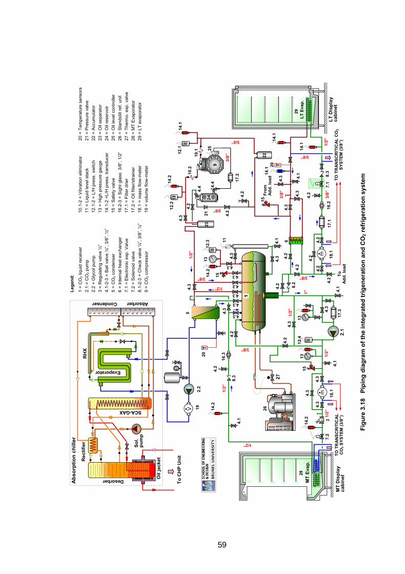
59

Fig

ure

3.1

8

Pip

ing

dia

gra

m o

f th

e in

teg

rate

d t

rig

ener

atio

n a

nd

CO

2 r

efri

ger

atio

n s

yste

m

LT

Dis

pla

y c

ab

ine

t

LT

Evap

. M

T E

va

p. R

ec

tifi

er

RH

X

Evaporator

Absorber Condenser

SCA-GAX

Desorber Oil

ja

ck

et

So

l.

pu

mp

Ab

so

rpti

on

ch

ille

r

2.2

V

m

TO

TR

AN

SC

RIT

ICA

L C

O2

SY

ST

EM

(3/

8”)

T

2.1

28

5

6

7.1

29

11

12.3

13

14.2

14.1

12.2

12.1

15

15

16.3

16.2

17.1

18.1

20

22

19

To

CH

P U

nit

T

20

26

27

1/2

”

1/2”

1/2

”

1/2”

MT

Dis

pla

y c

ab

ine

t

m

3

18.1

T

O T

RA

NS

CR

ITIC

AL

C

O2 S

YS

TE

M (

3/8

”)

17.2

3/8”

4.3

1/2”

5/8”

25

SC

HO

OL

OF

ENG

INEE

RIN

G

& D

ESIG

N

BR

UN

EL U

NIV

ER

SIT

Y

3/8”

3/8”

3/8

”

1/2

”

4.1

4.3

4.3

1”

24

21

4.3

4.2

4.3

4.2

4.2

4.3

8.2

4.2

4.2

4.2

4.3

4.3

4.3

4.3

23

1

4.2

10.2

10.1

4.2

4.3

4.3

4.3

4.2

4.3

4.3

4.3

13

4.3

15

4.2

9

3/8”

3/8

”

3/8”

4.4

4.4

8.3

1/2

”

1/2

"

4.1

4.1

4.2

4.1

14.2

14.1

14.1

14.2

14.2

1/2

”

4.2

14.1

4.1

1/2

”

3/8

”

4.2

4.2

8.3

12.4

13

17.3

7.2

To

A

dd

. lo

ad

Fro

m

Ad

d.

load

4.2

4.3

Leg

en

d:

1 =

CO

2 li

quid

rece

iver

2.1

= C

O2

pum

p

2.2

= G

lyco

l pum

p

3 =

Regula

ting

valv

e ½

”

4.1

-2-3

= B

all

valv

e ¼

”, 3

/8”,

½”

5 =

CO

2 c

ondense

r

6 =

Int

ern

al h

eat exc

hanger

7.1

= E

lect

ronic

exp

. V

alv

e

7.2

= S

ole

noid

valv

e

8.1

-2-3

= C

heck

valv

e ¼

”, 3

/8”,

½”

9 =

CO

2 c

ompre

ssor

10.1

-2 =

Vib

ratio

n e

limin

ator

11 =

Liq

uid

leve

l sta

ck

12.1

-2 =

L/H

pre

ss. sw

itch

13 =

Hig

h p

ress

ure

gauge

14.1

-2 =

L/H

pre

ss.

transd

uce

r

15 =

Saf

ety

valv

e

16.2

-3 =

Sig

ht

glass

3/8

”, 1

/2”

17.1

= F

ilte

r d

rie

r

17.2

= O

il fil

ter/

stra

iner

18.1

= m

ass

flo

w-m

eter

19 =

volu

me flo

w-m

eter

20 =

Tem

pera

ture

sens

ors

21 =

Pre

ssure

valv

e

22 =

Acc

umula

tor

23 =

Oil

separa

tor

24 =

Oil

rese

rvoir

25 =

Oil

leve

l co

ntr

olle

r

26 =

Sta

ndst

ill r

ef.

unit

27 =

Therm

o. e

xp.

valv

e

28 =

MT

Eva

pora

tor

29 =

LT

eva

pora

tor

60

Another common component is the liquid receiver where most of the CO2 refrigerant

charge is stored. The receiver and associated piping provide free flow of liquid from the

condenser. Pressures between the two are equalized so that the receiver cannot build up

a higher pressure than the condenser. To facilitate the flow of liquid CO2 from the

condenser by gravity, the condenser is placed just above the liquid receiver. A pipe from

the bottom of the receiver feeds liquid CO2 to the pump and LT DX systems. The pipe

has been sized to provide sufficient head for the CO2 pump and minimum pressure drop.

The liquid receiver is also equipped with an evaporator coil connected to a small

conventional condensing unit, as shown in Figure 3.18. The condensing unit is used to

keep the pressure of the liquid CO2 refrigerant low during standstill.

Figure 3.18 also shows pipe connections and flow control valves so that the loading

system and flow meters can also be used by a transcritical CO2 system. For safety, the

CO2 refrigeration system is equipped with safety relief valves. The location of the

valves can also be seen in Figure 3.18. Detailed description of the safety relief valves is

presented in Section 3.3.8. In addition, the piping system and components of the CO2

refrigeration system are also selected to be compatible with the CO2 refrigerant and

maximum pressure of at least 40 bar.

3.3.1 CO2 compressor

Selecting a CO2 compressor at the early stage of the development of the CO2

refrigeration technology was challenging due to limited range of capacities available.

Figure 3.19 shows the CO2 compressor selected for the test rig. It is a two-piston low

temperature semi-hermetic reciprocating compressor. It can be seen that at designed

conditions, Tevap = -32 oC and Tcond = -8 oC, the compressor has a refrigeration capacity

more than three times the designed load of the LT cabinet. Consequently, an additional

LT load was added to the test system to balance the load and to avoid the compressor

cycling on and off frequently. The compressor was also equipped with a variable speed

controller to enable some variation of capacity. Having a large capacity, the compressor

significantly increased the LT and MT load ratio. This subsequently reduced the overall

COP of the refrigeration system as previously demonstrated in Figure 3.11.

To ensure safe operation, the compressor was equipped with several safety controls

which included oil safety switch, low and high pressure switches, motor temperature

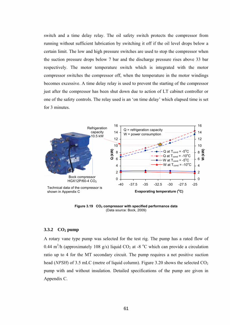
61

switch and a time delay relay. The oil safety switch protects the compressor from

running without sufficient lubrication by switching it off if the oil level drops below a

certain limit. The low and high pressure switches are used to stop the compressor when

the suction pressure drops below 7 bar and the discharge pressure rises above 33 bar

respectively. The motor temperature switch which is integrated with the motor

compressor switches the compressor off, when the temperature in the motor windings

becomes excessive. A time delay relay is used to prevent the starting of the compressor

just after the compressor has been shut down due to action of LT cabinet controller or

one of the safety controls. The relay used is an ‘on time delay’ which elapsed time is set

for 3 minutes.

Figure 3.19 CO2 compressor with specified performance data (Data source: Bock, 2009)

3.3.2 CO2 pump

A rotary vane type pump was selected for the test rig. The pump has a rated flow of

0.44 m3/h (approximately 108 g/s) liquid CO2 at -8 oC which can provide a circulation

ratio up to 4 for the MT secondary circuit. The pump requires a net positive suction

head (NPSH) of 3.5 mLC (metre of liquid column). Figure 3.20 shows the selected CO2

pump with and without insulation. Detailed specifications of the pump are given in

Appendix C.

0

2

4

6

8

10

12

14

16

-40 -37.5 -35 -32.5 -30 -27.5 -25Evaporating temperature (oC)

Q (

kW

)

0

2

4

6

8

10

12

14

16

W (

kW

)

Q_Tcon = -5oCQ_Tcon = -10oCW_Tcon = 5oCW_Tcon = 10oC

Q at Tcond = -5oC Q at Tcond = -10oCW at Tcond = -5oC W at Tcond = -10oC

Q = refrigeration capacity W = power consumption

Evaporating temperature (oC)

Bock compressor HGX12P/60-4 CO2

Technical data of the compressor is shown in Appendix C

Refrigeration capacity 10.5 kW

62

Cavitation in a CO2 refrigeration application is not a major problem due to energy

released during cavitation is much smaller compared to other refrigerants (Heerup,

2009). Cavitation, however, can reduce the specified flow capacity of a CO2 pump. In

order to avoid cavitation and to achieve the rated flow, the installation of the pump was

prepared to provide NPSH at least 3.7 mLC. In addition, heat transfer with the

surroundings on the suction pipe and the pump itself was also minimised by insulating

them with appropriate insulation as shown in Figure 3.20.

Figure 3.20 CO2 pump (Hermetic HTP 1-400)

The pump is also equipped with a safety control system which consists of a liquid level

relay, high pressure switch which switches the pump off when the discharge pressure

rises to 33 bar and a motor temperature switch. The liquid level relay is used to protect

the pump from cavitation by stopping the pump motor when the liquid level in the

liquid receiver drops to 35% of full liquid height.

3.3.3 Condenser

A plate type heat exchanger was selected as the condenser of the CO2 refrigeration

system. This type of heat exchanger has high thermal efficiency and small foot print

(Jokar et al., 2010). Figure 3.21 shows the condenser HX and its specifications. Detailed

size of the condenser is given in Figure C-3 (Appendix C).

The condenser is mounted in a counter flow configuration between the CO2 line and the

water-glycol line. The CO2 enters the condenser as a superheated gas at 6.3 oC and exits

Motor drive

The pump without insulation The pump with insulation

63

as saturated liquid at -8 oC. The temperature difference between the exiting liquid CO2

and returning water-glycol can be as low as 2 K (specified by the manufacturer).

Figure 3.21 CO2 condenser (SWEP B120THx60/1P-SC-M2)

3.3.4 Evaporators

Evaporator coils used in the loading system are standard finned coils which have been

designed to operate with CO2 refrigerant. The evaporator coil of the medium

temperature cabinet is a flooded coil whereas the coil for the low temperature cabinet is

a direct expansion coil.

Figure 3.22 shows the MT flooded coil fitted at the bottom of the MT cabinet. The coil

is made from copper tubes of 12.7 mm nominal outside diameter and corrugated

aluminium fins of 0.22 mm thickness and fin spacing of 158 fins per metre (FPM). The

coil consists of 4 circuits in staggered arrangement with 4 rows high, 6 rows deep and

total tube length of approximately 50 m. The MT coil can contain about 4.6 litres CO2

refrigerant.

Figure 3.22 also shows that the MT flooded evaporator coil is placed adjacent to the MT

DX evaporator coil which is used for transcritical CO2 refrigeration tests. The two

evaporator coils which are not used simultaneously are separated by a 25 mm air gap.

The size of the MT flooded coil is 152 x 198 x 2085 mm (height x depth x length). It is

relatively compact compared with a HFC evaporator coil of the same capacity. As it can

be seen from Figure 3.22, two CO2 MT evaporator coils could be fitted into the space

originally utilised by a single R-404A evaporator coil.

Parameters andspecifications

CO2 side

Water glycol side

Inlet temperature (oC) 6.3 -10 Outlet temperature (oC) -8 -6.8 Flow rate (kg/s) 0.040 0.725 Heat load (kW) 12 Heat transfer area (m2) 7.66 Over surface (%) 40 Number of channel 29 30 Test pressure (bar) 75 75 Max. working pressure (bar) 45 45 Hold up volume (L) 6.99 7.23

Without insulation With insulation

Condenser

64

The LT DX evaporator coil is also made from copper tube of 12.7 mm nominal outer

diameter with corrugated aluminium fins of 0.22 mm thickness. The fin spacing is 118

fins per metre (FPM). The coil comprises 3 circuits in staggered arrangement with 4

rows high and 8 rows deep and its size is 152 x 264 x 2030 mm (height x depth x

length). The total tube length is approximately 65 m which gives refrigerant volume of

about 6.1 litres. The LT evaporator coil is also utilised by the loading system of the

transcritical CO2 system. Both systems use a direct expansion coil for the low

temperature system and thus, only one LT evaporator coil is used. However, separate

evaporator controllers are employed for the two systems.

Figure 3.22 MT CO2 evaporator coils fitted in the display cabinet

The MT and LT evaporator coils were tested at 52 bar with specified maximum

allowable working pressure of 40 bar. Detailed information of the coils is given in the

technical drawings in Figures C-4 and C-5 (Appendix C).

To reduce the effect of frost formation on the coils the free flow area of the front part of

the coils was increased by reducing the fin density from 158 fins per metre to 79 fins

per metre for the MT coil (Figures 3.22 and C-4) and from 118 fins per metre to 59 fins

per metre for the LT coil (Figure C-5). The coils also utilise a hydrophilic coating on the

fins to improve condensate drainage and ease of separation of frost from the coil during

defrosting.

MT flooded evaporator coil for subcritical CO2 system

MT DX evaporator coil for transcritical CO2 test system

A

Details of A

158 FPM

79 FPM

158 FPM

79 FPM

Distributor and leading pipes

FPM = number of fins per metre; FPI = number of fins per inch; 158 FPM = 4 FPI; 79 FPM = 2 FPI

65

The main design parameters for the MT flooded coil are: CO2 saturated liquid enters the

coil at 28 bara ( -8 oC); evaporation temperature in the coil at -8 oC; CO2 exits the coil as

liquid and vapour mixture at vapour quality of 0.5 (at designed circulation ratio CR = 2).

For the LT evaporator coil, CO2 enters the EXV as liquid with 2.4 K subcooling at 28

bara. After expansion CO2 enters the LT coil as a liquid-vapour mixture at evaporation

pressure of 13 bara (-32 oC) and exits with 5 K superheating. Detailed designs of the

CO2 evaporator coils including simulation programmes which have been established to

evaluate their performance are presented in Chapter 4.

3.3.5 Expansion valve

Parameters considered in selecting and sizing the expansion valve for the low

temperature DX circuit were pressure drop across the valve of 15 bar, full load

refrigeration capacity of 3 kW and part load of 2 kW.

An electrically operated expansion valve

has been chosen for the DX evaporator

as shown in Figure 3.23. It has a wider

range and flexibility for refrigerant flow

control compared to the traditional

thermostatic expansion valve (TXV). It

also offers the possibility to integrate its

control with the cabinet controller to

make it easier to change the operational

settings for system investigations.

The valve is of the pulse-width-modulated type which is an on/off solenoid valve with

special features that allow it to operate as a variable metering device by rapidly pulsing

the valve open and closed. For example, if the evaporator needs 75% flow, the valve is

open 75% and closed 25% of the time. The duration of each pulse is regulated by an

electronic controller. Thus, the application of this valve requires a controller and control

sensors which include a pressure transducer and a temperature sensor. The controller of

the valve is integrated with the evaporator controller which is described in Sections 3.5

and 3.6.

Figure 3.23 Electronic expansion valve(Source: Danfoss, 2008)

Coil with DIN plug

Valve body complete with

orifice assembly

Orifice no. 2 (AKV10-2)

66

The expansion valve was specified to have a maximum operating pressure difference

(MOPD) across it of 18 bar and maximum operating pressure (MOP) of 52 bar.

Figure 3.24 Performance data of electronic expansion valves type AKV10 (Data source: Danfoss, 2008b)

Figure 3.24(a) shows the performance characteristics of the AKV10 range of valves. It

can be seen that the AKV10-2 is the closest AKV valve to satisfy the design

requirements. It can also be seen that the capacity of the AKV10 valve is much higher

when used with CO2 refrigerant compared to R-404A.

3.3.6 Internal heat exchanger

The internal or suction line heat

exchanger (IHX) is shown in Figure 3.25.

It is a plate heat exchanger and was

installed in counter flow configuration

between the liquid supply line and

suction line of the LT compressor. The

IHX can increase the degree of superheat

of the CO2 gas exiting the LT evaporator

to achieve suction superheating in the

range 8 to 12 K. It can also reduce the

risk of liquid entering the LT compressor. In the liquid line, the IHX subcools CO2

liquid entering the expansion valve and this can improve the COP of the LT system.

0

1

2

3

4

5

6

7

8

9

10

0 2 4 6 8 10 12 14 16 18 20

Pressure drop across valve (bar)

Re

frig

era

tio

n c

ap

ac

ity

(k

W) AKV10-1

AKV10-2AKV10-3AKV10-4

R-744

(a)

0

1

2

3

4

5

6

7

8

9

10

0 2 4 6 8 10 12 14 16 18 20

Pressure drop across valve (bar)

Re

frig

era

tio

n c

ap

ac

ity

(k

W)

AKV10-1AKV10-2AKV10-3AKV10-4

R-404A

(b)

Figure 3.25 Internal heat exchanger (SWEP: B5Hx10/1P-SC-M4)

IHX

Liquid line bypass valve

67

The IHX has a heat transfer capacity of 0.2 kW. The amount of subcooling can be

varied by using a bypass valve to bypass some of the refrigerant round the heat

exchanger.

3.3.7 Refrigerant flow control devices

Four types of flow control valves are used in the test system shown in Figure 3.26. They

are Danfoss products which are compatible with CO2 refrigerant. The solenoid and ball

valves are stop valves also commonly referred to as shutoff valves. The solenoid valve

was used to automatically prevent liquid CO2 flowing to the MT flooded evaporator

when no flow is required, such as during the defrost cycle and when the cabinet has

reached the set point. The ball valves are manually operated and used to isolate the

system components such as: compressor, pump, condenser, liquid receiver, IHX and

evaporators for servicing and safety (ASHRAE Standard 15, 2007).

Figure 3.26 Refrigerant flow control valves (Source: Danfoss, 2008b)

Ball valves were also installed on long lengths of pipe to isolate the system in case of

leaks and to facilitate pump down. The ball valves were also used to vary the flow

through components such as: IHX, pump and flow meters, by bypassing some of the

flow round the components.

A regulator valve is used in the MT circuit to regulate liquid CO2 flow to the MT

flooded evaporator. The valve is manually operated. Non-return valves are used to

prevent liquid from becoming trapped in pipe sections because when heated it can

expand rapidly and can reach pipe rupture pressure. A non-return valve is also fitted

Solenoid valve

Ball valves

Regulator valve

Non-return valve

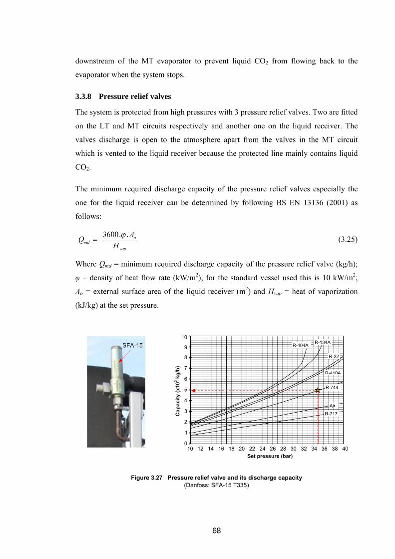
68

downstream of the MT evaporator to prevent liquid CO2 from flowing back to the

evaporator when the system stops.

3.3.8 Pressure relief valves

The system is protected from high pressures with 3 pressure relief valves. Two are fitted

on the LT and MT circuits respectively and another one on the liquid receiver. The

valves discharge is open to the atmosphere apart from the valves in the MT circuit

which is vented to the liquid receiver because the protected line mainly contains liquid

CO2.

The minimum required discharge capacity of the pressure relief valves especially the

one for the liquid receiver can be determined by following BS EN 13136 (2001) as

follows:

vap

omd H

AQ

..3600 (3.25)

Where Qmd = minimum required discharge capacity of the pressure relief valve (kg/h);

φ = density of heat flow rate (kW/m2); for the standard vessel used this is 10 kW/m2;

Ao = external surface area of the liquid receiver (m2) and Hvap = heat of vaporization

(kJ/kg) at the set pressure.

Figure 3.27 Pressure relief valve and its discharge capacity (Danfoss: SFA-15 T335)

10 12 14 16 18 20 22 24 26 28 30 32 34 36 38 40

Set pressure (bar)

10

9

8

7

6

5

4

3

2

1

0

R-404A R-134A

R-22

R-410A

R-744

Air

R-717Cap

acit

y (x

103 k

g/h

)

SFA-15

69

The pressure relief valve was set at a pressure 25% higher than the operating pressure of

the system giving a burst pressure of 35 bar. At this set pressure, the minimum

discharge capacity was determined to be 177 kg/h.

The characteristics of the pressure relief valve chosen for the application are shown in

Figure 3.27. The valve has a factory setting of 35 bar. It can be seen that discharge

capacity of the valve for CO2 application at this pressure is nearly 5000 kg/h which is

considerably higher than the 177 kg/h required.

3.3.9 Oil management system

The LT compressor inevitably loses some lubricating oil from the oil sump during

normal operation as some mixes and circulates with the refrigerant through the system.

In order to ensure that the majority of oil returns back to the compressor and to ensure

that the compressor is always properly lubricated; the CO2 refrigeration system is

equipped with an oil management system.

Figure 3.28 Schematic diagram and selected components of the oil management system

Figure 3.28 shows a schematic diagram of the oil management system and pictures of

the main components which include an oil separator, oil reservoir, oil strainer, oil level

regulator and a pressure valve. These components were specified for subcritical CO2

1 = Oil separator (OS-16-CD) 4 = Oil strainer (F-10L-CD)

2 = Oil reservoir (OSA-3.8-CD) 5 = Oil level regulator (ERM2-0-BC-CD)

3 = Pressure valve (RV-10B/1.5) = Ball valve

1 2

3

4

5

LT Compressor

Oil return line

4 Refrigerant line from evaporator

Refrigerant line to condenser

1 2

3

5 Accumulator

Oil check point

70

refrigeration applications with a maximum operating pressure (MOP) 40 bar except

from the oil separator which was specified for a MOP of 45 bar (ESK Schultze, 2008).

The oil separator has a capacity of 2.3 L with a first oil charge 0.6 L. The oil separator

removes some oil from the refrigerant and reduces the rate of oil circulation through the

refrigeration system. It is equipped with a built-in float valve which opens when the oil

level rises above the first charge level and the excess oil is drained back to the

compressor trough the oil reservoir.

The oil reservoir has a total volume of 3.8 L. It receives the returned oil from the oil

separator and also provides a reserve supply of oil for the compressor. It incorporates a

pressure valve (RV-10B/1.5) which maintains the pressure in the reservoir 1.5 bar

above the suction pressure. If the pressure rises above this value, the valve opens and

vents any refrigerant trapped with the oil back to the suction line of the compressor. The

oil reservoir also incorporates two sight glasses and two service valves. The sight

glasses are used to ensure that there is enough oil in the reservoir, while the service

valves are used for charging/draining the oil to/from the reservoir.

The oil supply to the compressor is regulated by the oil level regulator. The regulator

comprises an oil level sensor and a solenoid valve. The solenoid valve allows the

lubricating oil to flow to the compressor from the oil reservoir when the oil level

reaches its lower limit and stops the oil supply when the oil level reaches the upper

limit. The oil level regulator is also equipped with a relay which is integrated with the

compressor controller. The relay switch stops the compressor when the oil level drops

below the lower limit. The integration of the oil regulator relay with the compressor

controller is described in Section 3.5. The oil regulator relay is also used to activate an

alarm in the event the oil management system has failed to feed the lubrication oil into

the compressor.

3.3.10 Auxiliary components

Several auxiliary components associated with the main mechanical components of the

CO2 refrigeration system have been described previously. Other auxiliary components

are shown in Figure 3.29. These include an accumulator, sight glass, filter drier and

pressure gauges.

71

The suction line accumulator is an ESK product (FA-12-CD) specified for use with CO2

refrigerant. It has a 0.8 litre and a MOP of 40 bar. The accumulator protects the

compressor from damage by preventing liquid droplets from entering the compressor.

The system is also equipped with two sight glasses. One was installed on the liquid line

of the LT DX circuit to monitor the presence of flash gas upstream of the expansion

valve. Another sight glass was fitted on the MT secondary circuit to monitor the

refrigerant flow downstream of the MT flooded evaporator. Both sight glasses are

Danfoss products (type SGN) which are compatible with the CO2 refrigerant.

Figure 3.29 The auxiliary components

The filter driers used in the system are also Danfoss products (DCB bi-flow type). They

contain a mixture of silica gel and molecular sieves and are suitable for CO2 refrigerant

applications. They were installed on the liquid line, one upstream of the expansion valve

and another one upstream of the CO2 pump (Figure 3.18). The main purpose was to

limit any debris within the system from reaching the expansion valve and the CO2

pump. Using bi-flow type filter driers enables the liquid CO2 to flow in both directions

which can reduce the possibility of liquid being trapped in the system during standstill

conditions.

In order to monitor the pressure fluctuations during charging and operation, the test

system was also equipped with three pressure gauges. One was installed on the liquid

receiver and the other two upstream and downstream of the CO2 pump. The gauges are

Omega Engineering products (PG63-70S) compatible with CO2 refrigerant. They have a

measurement range from 0 to 70 bar. The gauges are very useful particularly when

 

Accumulator

Sight glass

Bi-flow filter drier

Pressure gauge

72

charging the CO2 system with refrigerant. The only way to immediately monitor the

pressure of the system is from the pressure gauges.

33..44 RReeffrriiggeerraattiioonn llooaadd ssyysstteemm

The test rig was originally designed for a full load refrigeration capacity of 8 kW

provided by two refrigerated display cabinets: a medium temperature cabinet of full

load capacity of 5 kW and a low temperature cabinet of full load capacity of 3 kW.

Because the lowest LT compressor capacity commercially available at the time the

system was designed was far bigger than the capacity of the LT cabinet as well as the

application of a variable speed controller could not reduce the compressor capacity as

low as the designed LT load; a low temperature additional load was added to the

loading system to balance the capacity of the compressor.

The effect of the additional load on the pressure drop of the LT piping system has also

been evaluated using the EES model. The pressure drops were still in the acceptable

range with pressure losses in the suction and liquid lines equivalent to saturation

temperatures 0.25 K and 0.04 K respectively.

3.4.1 Display cabinets

The refrigerated display cabinets used are a chilled open vertical multi-deck cabinet and

a glass door frozen food cabinet. They were originally designed for R-404A refrigerant

and were modified by replacing the evaporator coil and controls, to operate with CO2

refrigerant. The evaporator coil of the low temperature cabinet is a direct expansion coil

whereas the coil of the medium temperature cabinet is a flooded evaporator coil which

was designed to operate with CO2 as a secondary (volatile) refrigerant.

The chilled or MT cabinet is a Carter ELFM 2.54 m long cabinet with an open length

2.47 m. The height of the cabinet is 2.05 m and the depth 1.13 m. The cabinet has a total

display area (TDA) of 4.2 m2. The flooded evaporator coil and circulation fans are

located below the base shelf. A schematic diagram of the MT cabinet is shown in Figure

30 (a). It can be seen that the cabinet has two evaporator coils as previously explained in

Section 3.3.4.

Figure 3.30 (b) shows a schematic diagram of the glass door frozen food cabinet. It is a

2.4 m long display cabinet with glazing height of 1.9 m and display area of 2.7 m2. The

73

three glass doors of the cabinet incorporate anti-sweat heaters to prevent condensation

(sweating) on the glass surface.

Figure 3.30 Refrigerated display cabinets

The cabinets were loaded with test packages stacked on the shelves. The test packages

of the MT cabinet were 0.8 litre plastic containers filled with water. For the LT cabinet,

one litre plastic containers filled with 50% propylene glycol in water solution were

used. The solution has a freezing temperature of -33 oC. At the positions where product

temperatures were measured, M-packages were used according to ISO 23953-2 (2005).

Each M-package had a calibrated T-type thermocouple inserted into the geometric

centre of the package.

3.4.2 Low temperature additional load

The additional load comprises an evaporator heat exchanger, water-glycol circuit and

auxiliary components. The loading system is also used for additional load of the

transcritical CO2 system. A schematic diagram of the additional load, including the

connections to the subcritical and transcritical CO2 test systems, is shown in

Figure 3.31.

The evaporator HX of the additional load system is a plate type heat exchanger (PHX)

SWEP-B15Hx30/1P-SC-M of 8 kW refrigeration capacity at evaporating temperature

-32 oC and 10 K superheat. The cold-stream of the heat exchanger functions as a CO2

(a) MT display cabinet

14002050

1126

6 fans

MT flooded evaporator coil

MT DX evaporator coil

300

 

2015

907 975

1450

3 fans

LT DX evaporator coil

(b) LT display cabinet

74

LT DX evaporator which absorbs heat from water-glycol solution at the hot-stream of

the heat exchanger. The evaporator HX incorporates a “Danfoss” cabinet controller

AK-CC 550A, electronic expansion valve (AKV10-4), pressure transducer (AKS-32)

and temperature sensors type PTC-1000 (AKS-11). Operational settings of the

evaporator including the refrigerant superheat can be set in the AK-CC 550A controller.

Figure 3.31 Schematic diagram of the LT additional load

The refrigerant circuit of the additional load also incorporates auxiliary components

such as sight glass, filter-drier and flow control valves (SV, NRV and BV) as shown in

Figure 3.31. The solenoid valve (SV) is used to regulate the flow to the evaporator HX.

This valve automatically closes when the temperature set point has been achieved. The

non-return valve (NRV), also known as check valve, is fitted in parallel with the

solenoid valve to allow the liquid CO2 to escape when the valve is closed. This protects

the circuit from damage that may be caused by liquid CO2 trapped in the pipe. The ball

valves (BV) are utilised to enable the additional load to be used by both the subcritical

and transcritical CO2 test systems.

The water-glycol circuit consists of a circulation pump and a water storage tank. The

circuit was filled with propylene glycol of 55% mass fraction in water solution.

LT Evaporator HX m

T

T

T

T

AKV

Mass flow meter

SG

SV

NRV

BV Transcritical CO2 system

Subcritical CO2 system

BV

Water Pump

Water storage tank 100 litres

Filter-drier

Immersion heaters 8 kW

EKC-101 AK-CC 550A

~

AC 240 V

75

The solution has a freezing temperature of -38 oC. The purpose of using this high

concentration solution is to prevent ice blockage in the channels of the evaporator plate

heat exchanger due to low evaporating temperature.

The circulation pump used in the water-glycol circuit is a Grundfos CH-2-30 specified

for a flow capacity of 1.5 m3/h; total head 30 m and minimum operating temperature

-20 oC. Water storage is provided by a 100 litre copper tank insulated with polyurethane

foam of 50 mm thickness. The storage incorporates two immersion heaters of heating

capacity 4 kW each and a temperature controller Danfoss EKC 101. The temperature of

the water-glycol mixture at the outlet of the storage tank is maintained relatively

constant by regulating the power supply to the immersion heaters. In addition, the

circuit also incorporates a flow meter to measure the flow rate of the water-glycol

mixture. This flow rate was used to determine the refrigeration duty of the additional

load system.

33..55 CCoonnttrrooll ssyysstteemm

Figure 3.32 shows a schematic diagram of the control system which consists of

electrical and electronic control systems. The electrical control system comprises an LT

control circuit (C-1), MT control circuit (C-2) and standstill control circuit (C-3). The

main function of the electrical control system is to connect and to disconnect power

supply to the electrical components as well as the electronic control system. The LT

control circuit (C-1) automatically regulates the operation of the LT compressor based

on inputs from the LT cabinet controller, high and low pressure switches and oil level

regulator. The MT control circuit (C-2) drives the CO2 pump including the solenoid

valve upstream of the MT evaporator. The control circuit receives input from the MT

cabinet controller, discharge pressure switch and liquid level controller. The standstill

control circuit (C-3) energises the standstill condensing unit based on the pressure of the

liquid receiver during standby conditions. The following sections detail the electrical

and electronic control systems including the control strategy applied to the test rig.

3.5.1 The electrical control system

Wiring diagrams of the electrical control system are given in Figures D-1 to D-5

(Appendix D) which detail the electrical installation of the main control circuit followed

by LT, MT, standstill and additional load control circuits respectively.

76

Fig

ure

3.3

2 S

chem

atic

dia

gra

m o

f th

e el

ectr

ical

an

d e

lect

ron

ic c

on

tro

l sys

tem

s

V45

LT

Dis

pla

y ca

bin

et

Rec

tifi

er

RH

X

Evaporator

Absorber Condenser

SCA-GAX

Desorber Oil

jac

ket

So

l. p

um

p

Ab

sorp

tio

n c

hil

ler

Gly

col

pu

mp

V

m

TO

TR

AN

SC

RIT

ICA

L C

O2

SY

ST

EM

(3/

8”)

T

Co

nd

ense

r

IHX

EX

V

Liq

. le

vel

tran

smit

ter

Cu

t in

30

bar

P

S3

PS

6

35

bar

35 b

ar

Fil

ter/

dri

er

Flo

w

met

er

Flo

w

met

er

Sta

nd

still

co

nd

ensi

ng

un

it

MT

Dis

pla

y ca

bin

et

m

V38

V20

V37

V

35

V36

V15

V02

V18

V17

V

19

V23

V11

V10

Rec

eive

r

V26

V06

V07

V08

V09

V05

V01

PS

9

PS

8

T

PS

5

PS

4

V12

V

14

Cu

t o

ut

34 b

ar

PS

2

Cu

t o

ut

8 b

ar

PS

1

V27

V04

35 b

ar

Cu

t o

ut

34 b

ar

Pu

mp

V28

PS

7

LT

1

LT

2 V30

V29

V31

V32

V16

V13

V22

V44 V24

V25

Fil

ter/

dri

e r

V33

Co

mp

ress

or

V34

V39

V40

V03

V41

V42

TO

TR

AN

SC

RIT

ICA

L

CO

2 S

YS

TE

M (

1/2”

) V

43

V21

To

Ad

d.

loa

d

V47

Fro

m

Ad

d.

load

Flo

w

met

er

R22

R9

R11

LT2

C-2

EK

C 4

14A

1

D

F

L/A

C-1

T

TT

EK

C 3

47

EK

C 1

01

D

F

L/A

EK

C 2

04A

1

C-3

T

T

T

SC

HO

OL

OF

ENG

INEE

RIN

G

& D

ESIG

N

BR

UN

EL U

NIV

ER

SIT

Y

SV

OL

R

=

Pre

ssu

re s

witc

h

=

Pre

ssu

re t

rans

duc

er

=

Te

mpe

ratu

re s

ens

or

EX

V =

Ele

ctro

nic

exp

. va

lve

S

V =

Sol

eno

id v

alv

e

C-1

= C

om

pre

sso

r co

ntro

l C

-2 =

CO

2 p

ump

con

tro

l C

-3 =

Sta

ndst

ill c

ontr

ol

D =

De

fro

st c

on

trol

F

= F

an

con

tro

l L

= L

igh

ting

co

ntr

ol

A =

Ala

rm

EK

C 1

01

= T

em

p. c

ontr

olle

r E

KC

20

4A

1 =

Vo

latil

e

e

vap

orat

or

con

tro

ller

EK

C 3

47

= L

iqui

d le

vel c

ont

rolle

r E

KC

41

4A

1 =

LT

-eva

po

rato

r

c

ontr

olle

r O

LR

= O

il le

vel r

egul

ator

Leg

end

:

T

77

Figure D-1 (Appendix D) shows the wiring diagram of the power supply to the

compressor, CO2 pump, LT, MT and standstill control circuits. Each circuit is protected

against overload or short circuit conditions using a circuit breaker. The whole circuit is

isolated by a main switch and an emergency switch. The electrical system also

incorporates a residual current device (RCD) which is an electrical wiring device that

disconnects the main power supply to the whole system whenever it detects current

leakage through the human body that is grounded and accidentally touching the

energised part of the circuits.

The LT and MT control circuits are detailed in Figures D-2 and D-3 (Appendix D). It

can be seen that the operation of the LT compressor and the CO2 pump are regulated

through using contactor relays. The relay of the LT compressor is circuited in series

with the control switches of the LT cabinet controller; high and low pressure switches

and oil regulator (Figure D-2). The CO2 pump relay (Figure D-3) is energised by the

contact switches of the MT cabinet controller, discharge pressure switch and liquid level

regulator. Both contactor relays can also be manually overridden by on/off switches.

The figures also show that the controls of the LT and MT cabinets have been modified

to incorporate the installation of a selector switch in each display cabinet to switch over

the connection of the cabinet controller either to the subcritical or transcritical CO2

systems. The modified control also incorporates three switches to override the

automatic on/off inputs from the cabinet controller to the fans, lights and defrost heater

respectively.

3.5.2 The electronic control system

The system employed is a commercially available electronic control system

manufactured by Danfoss. Figure 3.33 shows the electronic controllers used which

consist of an LT cabinet controller (EKC-414A1), MT cabinet controller (EKC-204A1),

water-glycol temperature controller (EKC-101) and liquid level controller (EKC-347).

The system also uses an AK-CC 550 controller to control the additional load evaporator

as explained in Section 3.4.2.

The cabinet controller EKC-414A1 automatically regulates the operation of the LT

cabinet based on parameter settings and input signals from the sensors. The operational

parameter settings, which can be set by using a panel mounted display EKA-162,

78

include temperature set point, temperature range, degree of superheat and defrost

parameters (type, frequency, duration and temperature termination). The controller

receives input signals from a suction line pressure transducer and temperature sensor

fitted on the outlet of the evaporator. The controller also detects temperatures of the air

in the LT cabinet from PTC-1000 type temperature sensors which were placed on the

air-on, air-off and on the free surface of LT evaporator coil. The controller modulates

the opening of the expansion valve to provide the specified degree of superheat at the

outlet of the LT evaporator. To ensure the controller can provide an accurate modulation

to the expansion valve, the refrigerant used in the system (R-744) and the pressure range

of the pressure transducer must be specified correctly in the controller. The controller

also provides an on/off signal to the LT control circuit to control the operation of the LT

compressor. A wiring diagram showing the controller, location of the sensors and their

connections is shown in Figure D-6 (Appendix D).

Figure 3.33 Control components (Source: Danfoss, 2008b)

The MT cabinet controller (EKC-204A1) is simpler compared to the DX evaporator

controllers. The controller provides on/off signal to the fans, lights and defrost heater of

the cabinet without controlling the degree of superheat of the refrigerant. Thus, it

requires only input signals from temperature sensors which include air on, air off and

MT evaporator coil surface. Together with the liquid level controller (EKC-347), the

EKC-204A1 regulates the operation of the CO2 pump and the solenoid valve upstream

of the MT evaporator coil.

The electrical power of both LT and MT controllers (EKC-414A1 and EKC-204A1) is

supplied from the electrical control system through selector switches. These switches

EKC-347 EKC-414A1 EKC-101

EKC-204A1

79

can be used to drive the controllers either manually or automatically. For the automatic

control operation, the switches were fitted in series with contact switches of a

temperature controller EKC-101. This temperature controller is used to prevent the CO2

system from operating when the temperature of the water-glycol, which cools the CO2

condenser, is still high, above -3 oC. This setting can, however, be varied to allow CO2

system performance investigations at different condensing temperatures.

Figure 3.34 Electrical control panel

The electrical and electronic control systems were installed in an electrical control panel

on the compressor-pump section of the test rig. A front view of the control panel

showing controller displays, switches and indicator lights is shown in Figure 3.34 (a)

and the arrangement of the components inside the panel can be seen in Figure 3.34 (b).

3.5.3 Control strategy

Figure 3.35 shows the control strategy applied to the test rig. The flow temperature

delivery from the trigeneration system is maintained relatively constant by using the

1

3

5

6

7

8

11

10

(a) (b)

4

Legend: 1 = main switch 6 = switches for EKC-414A1, EKC-204A1, EKC-101 2 = compressor speed controller 7 = controllers’ display 3 = power latch 8 = power supply indicators 4 = switches for: LT control system, 9 = contactor relays compressor, standstill condensing unit, 10 = LT cabinet controller EKC-414A1 MT control system and CO2 pump 11 = liquid level controller EKC-347 5 = emergency switch 12 = circuit breakers and RCD

2

9 12

80

temperature controller (thermostat) of the absorption system. In normal operation, the

delivery water-glycol temperature was set at -10 oC with 0.5 K temperature differential.

The MT system control strategy involves the control actions of the pump control circuit,

EKC-347 and EKC-204A1. The EKC-347 modulates the pump control circuit to allow

the pump to operate when the liquid level in the liquid receiver above 35% of full liquid

height. The EKC-204A1 also provides signal to the pump control circuit to regulate the

pump operation based on air temperatures in the MT cabinet which were set at -3 oC

weighting 100% air-off temperature with 2 K differential. The pump control circuit

switches the pump off when the air-off temperature reaches -3 oC and allows it to

operate again when the air-off temperature rises to -1 oC. The MT system incorporates a

solenoid valve upstream of the MT evaporator. The pump will operate after the solenoid

valve to be energised with a time delay of 1 minute and the pump will turn off 1 minute

before the valve is deenergised.

Figure 3.35 also shows the control strategy for the LT system which comprises

compressor and LT load control. The compressor control strategy is based on the

suction pressure of the LT compressor. The main parameters that affect the suction

pressure are the LT refrigeration load and the compressor flow capacity. At full load

conditions, the flow capacity of the compressor can maintain the target pressure at 12.2

bar. At part load conditions, however, the flow capacity of the compressor must be

modulated by varying its speed using a frequency inverter.

The LT load control strategy involves the control of the LT cabinet and LT evaporator

for additional load involving controller EKC-414A1 and AK-CC 550 respectively. The

controllers modulate the opening of the respective expansion valves to maintain a

degree of superheat in the range 5 K to 12 K. At full load conditions, the valve opening

was set at 80% of maximum represented by the pulsing frequency of the valve solenoid.

The EKC-414A1 also provides input signal to the compressor control circuit to regulate

the speed of the compressor. The control regulation is based on average air on and air

off temperature of the evaporator of -23 oC and a differential of 4 K. The AK-CC 550

controls the solenoid valve upstream of the additional load evaporator. The valve is

closed when the temperature of the water-glycol exiting the evaporator drops below

-27 oC.

81

Figure 3.35 Operational control strategy

RV

AKV10-2 LT Compressor

MT Cabinet

LT Cabinet

T

Compressor control circuit

12.2bar

5-12K

80 %

-3 oC

Air off 100%

-23oC

Air off 50%

AKV10-4

AK-CC 550A

T EKC-101

Brine-2 temperature T

Valve opening

LT additional load evaporator

Degree of superheat

12.2bar

5-12K

80 % -13

oC

Additional load system

Valve opening

CO2 Pump

On-Off

Trigeneration

system

Thermostat of the Absorption chiller

Brine-1 temperature

T

-10 oC

EKC-204A1

On-Off

Liquid receiver

= pressure transducer

Pump control circuit

EKC-347

min. 35%

On-Off

SV

T = temperature sensor

Brine is propylene glycol in water solution; brine-1 = 40% and brine-2 = 55%; SV = solenoid valve; NRV = non-return valve; RV = regulator valve

Degree of superheat

Compressor speed

Frequency inverter

EKC-414A1

On-Off

NRV

SV

T

-27oC

Fans Lights Heater

FansLights

Heater

Water-glycol out 100%

82

33..66 IInnssttrruummeennttaattiioonn aanndd ddaattaa llooggggiinngg ssyysstteemm

The instrumentation is used for both control and performance monitoring. For control,

the instrumentation is mainly used to provide signal inputs to the controllers. For

monitoring, the instrumentation is used to establish the state and flow conditions of the

CO2 refrigerant such as pressure, temperature and flow rate at different points in the

system. The instrumentation is also used to monitor the liquid level in the liquid

receiver, temperature and relative humidity of the loading system and test chamber as

well as power consumption of the test rig. To enable the information to be read and

recorded for system analyses and evaluation, the instrumentation is connected to a data

logging system.

3.6.1 Instrumentation devices

The instrumentation devices used on the test rig are temperature and pressure

measurements, liquid level transducer, relative humidity sensor, flow meter, and power

meter. A velocity meter was also used to measure air velocity in the test chamber and

MT display cabinet. The following sections provide a brief description of each device.

3.6.1.1 Temperature and pressure measurements

T-type thermocouples were used for most of the temperature measurements. The

thermistors (thermally sensitive resistor) type PTC-1000 were used for the sensors of

the control system and RTDs (resistance temperature detector) for the air temperature

sensor of the test chamber. T-type thermocouples have a temperature measurement

range -250 oC to 350 C with specific error (specified by manufacturer) of ± 0.5 oC. The

thermocouples were calibrated using a calibration bath and precision thermometer (ASL

type F250 MK II, probe J 100-250-10-NA) of uncertainty ± 0.04 oC. The temperature

range of calibration was -30 oC to 100 oC. It was found that all thermocouples had

calibration error within the specifications.

Positions of the temperature measurements on the test rig are indicated in Figure E-1

(Appendix E). The number and explanation of each measurement point are listed in

Table E-1 and the calibration equations of the thermocouples including their calibration

errors are given in Table E-2 (Appendix E).

83

Ten pressure transducers (Danfoss products) were installed on the test rig. One type

AKS 32 with output voltage 0-10 V d.c. is used for the control system. The others are

used to measure the pressures in the suction and discharge lines of the compressor and

CO2 pump, upstream and downstream of the LT and MT cabinets as well as the

pressure in the liquid receiver. Measurement points of the pressure transducers are

shown in Figure E-1 (Appendix E).

The pressure transducers of the monitoring system have different measurement ranges

with input voltage of 24 V d.c. and output current 4 mA to 20 mA. The output cables of

the transducer have to be circuited with a resistor to change the output current to

become an output voltage since the data logging system requires a voltage input. The

pressure range of the transducers and the resistors used are given in Table E-3

(Appendix E). Each pressure transducer of the monitoring system was calibrated using

a deadweight pressure gauge calibrator. The voltage outputs were recorded for a series

of known pressures. The graphs of the voltage against the pressure were drawn and the

best-fit linear equations were derived and used in the data logging system to enable an

automatic recording of the measured pressures. The coefficient of correlations of the

pressure transducers were above 99.9% with manufacturer uncertainty of ± 0.3%.

The graphs and calibration equations of the transducers are given in Figure E-3

(Appendix E).

3.6.1.2 Liquid level transducer

The transducer used is AKS 41U-15.3 which is a Danfoss control component. It has an

insertion rod length of 389 mm and was calibrated for water (R-718) with 4 to 20 mA

output across the whole measuring range. Before installation, the transducer was

recalibrated using water to set the minimum and maximum levels which provided a

measurement range as high as the internal diameter of the liquid receiver (310 mm). The

setting was then adjusted for CO2 (R-744). Figure 3.36 shows the transducer and its

electrical connection to the liquid level controller EKC 347. The level of the liquid CO2

in the receiver can be read on the display of the controller as a percentage of the total

measurement range. The reading can also be recorded and displayed on the screen of the

data logging system.

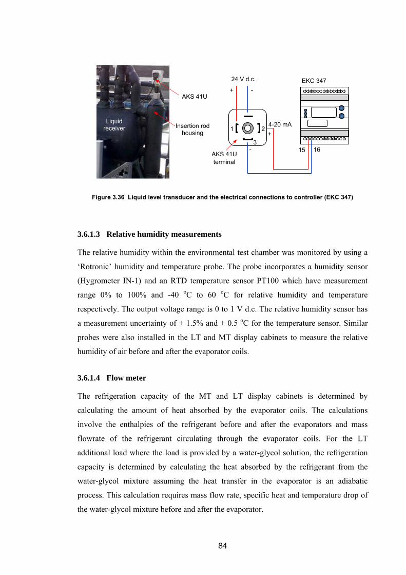
84

Figure 3.36 Liquid level transducer and the electrical connections to controller (EKC 347)

3.6.1.3 Relative humidity measurements

The relative humidity within the environmental test chamber was monitored by using a

‘Rotronic’ humidity and temperature probe. The probe incorporates a humidity sensor

(Hygrometer IN-1) and an RTD temperature sensor PT100 which have measurement

range 0% to 100% and -40 oC to 60 oC for relative humidity and temperature

respectively. The output voltage range is 0 to 1 V d.c. The relative humidity sensor has

a measurement uncertainty of ± 1.5% and ± 0.5 oC for the temperature sensor. Similar

probes were also installed in the LT and MT display cabinets to measure the relative

humidity of air before and after the evaporator coils.

3.6.1.4 Flow meter

The refrigeration capacity of the MT and LT display cabinets is determined by

calculating the amount of heat absorbed by the evaporator coils. The calculations

involve the enthalpies of the refrigerant before and after the evaporators and mass

flowrate of the refrigerant circulating through the evaporator coils. For the LT

additional load where the load is provided by a water-glycol solution, the refrigeration

capacity is determined by calculating the heat absorbed by the refrigerant from the

water-glycol mixture assuming the heat transfer in the evaporator is an adiabatic

process. This calculation requires mass flow rate, specific heat and temperature drop of

the water-glycol mixture before and after the evaporator.

24 V d.c.

+ -

1 2

3 15 16

4-20 mA

-

+

EKC 347

AKS 41U terminal

Liquid receiver

AKS 41U

Insertion rod housing

85

To ensure that the mass flow rates are measured with reasonable accuracy, a coriolis

type flow meter was chosen for the CO2 refrigerant and an electromagnetic flow meter

was used for the water-glycol mixture. Figure 3.37 shows the flow meters employed in

the test rig. For the LT display cabinet which requires a CO2 mass flow rate of about

0.011 kg/s, the Optimass-3050C-S03 (Figure 3.37a) is used which has a flow rate

capacity up to 0.028 kg/s. The Optimass-MFM-4065 (Figure 3.37b) with a

measurement range up to 0.342 kg/s is used for the MT display cabinet. Both flow

meters were manufactured by Krohne-Germany and have a measurement uncertainty of

± 0.035%. The flow meters, however, are also subject to inaccuracies arising from the

presence of gas bubbles in the liquid line. To minimise the risk of this occurring, the

liquid line was insulated with 25 mm of insulation (Armaflex class 0) and a liquid

suction HX was installed in the LT system.

Figure 3.37 Flow meter of the LT, MT and additional load systems

The Aquaflux-2010-IFC-010D meter shown in Figure 3.37c, also from Krohne, is used

to measure the volume flow rate of the water-glycol mixture. The volume flow rate was

converted to mass flow rate by multiplying it with the density of the water-glycol

mixture determined using the bulk mean temperature of the mixture in the evaporator.

The flow meter has a capacity range 0.5 to 21 m3/h and uncertainty ± 0.3%.

Each flow meter provides a current output 4-20 mA which is converted into a voltage

input in the data logging system. In order to convert the voltage to a flow rate, a

(b) Coriolis flow meter, Optimass-MFM-4065

(a) Coriolis flow meter, Optimass-3050C-S03

(c) Electromagnetic flow meter Aquaflux 2010-IFC 010D

86

calibration was carried out in the laboratory. Best-fit linear equations from the

calibration were used in the logging programme to enable automatic recording of flow

rate.

3.6.1.5 Power meter

The power consumption of the CO2 test

rig includes the power of the LT

compressor, CO2 pump, and the control

system. In order to measure these, a

power meter was installed in the electrical

control panel. The power consumption of

the control system was determined when

both compressor and pump were in off-

cycles and the power consumption of the

compressor and pump were determined when only one of them was in operation. The

power meter used is a Voltech PM-300, shown in Figure 3.38. It is a three phase power

analyser which has measurement uncertainty for voltage and current of ± 0.02% and

± 0.03% respectively. The power meter has an LCD screen to display the measured

voltage, current, power factor, and instant power. The measured parameters were also

logged into the computer via RS232 port.

3.6.1.6 Velocity meter

The velocity meter was used to map the velocity profile of the air flow in the

environmental test chamber to ensure that the air velocity was within the ISO 23953-2

standard. The meter was also used to measure the air velocity at the back tunnel of the

MT cabinet which is required for determination of the mass flow rate of the air flow

across the MT evaporator coil. The air mass flow rate was used to verify the

refrigeration capacity of the MT flooded evaporator coil when the circulation ratio of

the MT circuit was equal to 1. The velocity meter is Velocicalc Plus 8386A-M-GB, a

TSI product, with measurement range 0 m/s to 50 m/s and uncertainty ± 3%. The meter

can also simultaneously measure the temperature and relative humidity of the air with

measurement range -10 oC to 60 oC and 0% to 90% RH respectively.

Figure 3.38 Power meter, Voltech PM-300

87

3.6.2 Data logging system

The output signals from the instrumentation devices are logged by a data logging

system which comprises data acquisition modules and a recording and display system.

The data acquisition modules utilise the Datascan 7000 series from MSL (Measurement

System Ltd.) which include a Datascan measurement processor 7320 and expansion

modules 7020. Each Datascan module contains 16 differential input channels,

individually configurable for voltage and thermocouple measurements. To cover all the

instrumentation devices used, 1 processor and 11 expansion modules were prepared as

shown in Figure 3.39a. The configuration of each module and the channels are detailed

in Table E-1 (Appendix E).

Figure 3.39 Data logging system

The recording and display system is a standard desk top computer. Communication

between the Datascan modules and the computer is performed through an RS232 cable.

The computer incorporates Labtech software which is fully compatible with the

Datascan modules and allows a mix of more than 250 analogue and digital channels.

The software also has a capability to manipulate a complex measurement system to be

an attractive display so that it can be easier to monitor. The power consumption of the

test rig was recorded and monitored separately using a second computer set. Both

(b) Computer sets (a) Datascan processor and expansion modules

Power supply 24 V d.c.

Processor Datascan 7320

11 extension modules,

Datascan 7020

Additional power supply 24 V d.c.

.for the instrumentation

devices

88

computer sets are shown in Figure 3.39b. A monitoring display set up in the Labtech

software is given in Figure E-2 (Appendix E).

33..77 RReeffrriiggeerraanntt cchhaarrggee

The test rig is equipped with two charging connections, one is in the suction line of the

LT compressor and the other is downstream of the MT evaporator just before the

connection to the liquid receiver. This enables the system to be charged in gas or liquid

phase. Figure 3.40 shows one of the charging connections and valve. The charging

valve is used to isolate the system when the charging process has been completed.

Figure 3.40 CO2 and charging connection

Before charging, the system was pressure-tested and then evacuated. The system was

charged during standstill conditions directly to the liquid receiver. Two methods of

charging were used. Firstly, charging in gas when the system was in vacuum conditions

until the pressure reached 7 bar (slightly above the triple point of CO2). This prevents

the formation of dry ice which can block the charging line when charging in liquid. The

outlet valves of the liquid receiver were open to allow the whole CO2 system to be

pressurised. Secondly, charging in liquid. All outlet valves of the liquid receiver were

closed. The standstill condensing unit was set in automatic operation. The condensing

unit operates when the pressure in the liquid receiver increases to 30 bar. The level of

liquid CO2 in the liquid receiver can be monitored from the display of the EKC-347.

Charging valve

Charging connection

CP grade CO2

Refrigerant grade CO2

89

The amount of refrigerant charge is 37 kg which fills 50% of the receiver volume with

liquid CO2. This gives a specific refrigerant charge of 2.3 kg/kW which is in the range

of the charge of a centralised supermarket CO2 system as reported in MTP (2008).

The CO2 used in the system is of refrigerant grade. The cylinder of the refrigerant grade

CO2 is shown in Figure 3.40. Alternatively, a CP (Chemically Pure) grade CO2 with

100% purity can also be used (Figure 3.40). Both have the same characteristics. The

price of the CP grade CO2, however, is 16% lower than the refrigerant grade CO2.

33..88 EEnnvviirroonnmmeennttaall tteesstt cchhaammbbeerr

The display cabinets of the refrigeration load system were placed in an environmental

test chamber which is a self contained unit located near the CO2 plant room. Figure 3.41

shows a picture of the test chamber and the site where the test chamber is located. It can

be seen that the test chamber is situated outside and the fluctuation of ambient

conditions can directly affect its thermal load. In order to control the air temperature and

relative humidity as well as the air velocity, the chamber incorporates an air handling

unit (AHU) which was installed above its roof and supported by a purpose built steel

structure. Figure 3.41 also shows other facilities surrounding the test chamber which

include CO2 plant room and CHP chamber.

Figure 3.41 CO2 test chamber and associated test facilities

AHU

Condensing unit

CO2 test chamber

CO2 plant room

CHP chamber

Liquid receiver section

Humidifier

90

The layout and detailed dimensions of the test chamber are given in Figure F-1

(Appendix F). The external walls of the test chamber, also known as non-technical

walls, are constructed from steel frames and covered with painted metal skins. The gap

between the metal skins was filled with a rock-wool layer which provided a total wall

thickness of 80 mm and a U-value (thermal transmittance) of 0.5 W/m2K. The roof and

the suspended floor have a similar structure of 125 mm thickness with a U-value of 0.4

W/m2K. The chamber also has a single glazed window of U-value 5.7 W/m2K and a

swing door, 0.9 m wide and 2.5 m high. In order to provide access to bring the cabinets

into the chamber, an extension door with screw joints was constructed adjacent to the

swing door giving a total opening of 2.5 m wide and 2.5 m high.

Figure 3.42 Technical walls of the CO2 test chamber

Both ends of the chamber where the supply and return AHU ducts terminated were

partitioned off with technical walls to form supply and return air plenums. This provides

a maximum useful test area of 6.14 m long, 3.1 wide and 3.05 m high. The technical

walls of the supply and return air plenums were constructed from perforated plate

supported by a wooden frame. The walls are also covered with air filters to provide a

pressure drop and uniform air velocity across the technical walls as well as within the

test area. A polyester fibre air filter giving a pressure drop between 135 Pa and 250 Pa

and a glass fibre panel air filter of 10 to 125 Pa pressure drop were used to cover the

supply air and return air perforated plates respectively. Figure 3.42 shows the

construction of the technical walls viewed from the test area.

(a) Supply air technical wall (b) Return air technical wall

Perforated plate with

polyester fibre air filter

Perforated plate with glass

fibre air filter

91

3.8.1.1 Positioning the display cabinets in the test chamber

Figure 3.43 shows the positions of the MT and LT cabinets inside the chamber. It can

be seen that the MT cabinet is placed near to the return air technical wall and the LT

cabinet 0.5 m away from the supply air technical wall. The location of the cabinets in

the chamber is given in Figure F-2 (Appendix F).

Figure 3.43 Position of the MT and LT cabinets in the test chamber

3.8.1.2 Air handling unit

Figure 3.44 shows a schematic diagram of the air handling unit (AHU). The AHU is a

weatherproof model CAIRplus-128-096AVBV from GEA-Denco Ltd. specified for

outdoor installation with a design duty of 1.9 m3/s and 400 Pa pressure drop. It

comprises a mixing section, air filter, cooling coil, electric heater battery, heating coil,

humidifier section and a centrifugal fan. The unit is connected to the return air and

supply air plenums by return and supply air ducts respectively.

The mixing section of the AHU constitutes a return air damper and a fresh air damper to

facilitate control and regulations of the return and fresh air to the unit. The filter section

contains cardboard-framed synthetic panel and plastic-framed synthetic bag filters. The

section is also completed with two gauge manometers to measure the pressure

difference before and after the filters. Start pressure drops of the panel and bag filters

(a) The MT cabinet and the return air technical wall

(b) The LT cabinet and the supply air technical wall

Return air technical wall

MT cabinet

Supply air technical wall

LT cabinet

92

are 58 Pa and 98 Pa respectively and the filters must be replaced when the pressure drop

reaches 200 Pa for the panel filter and 300 Pa for the bag filter.

The cooling coil is a DX evaporator coil manufactured from copper tubes and

aluminium fins of 3.5 mm fin spacing. The evaporator coil has three circuits and two

rows arrangement with refrigerant volume of 6 litres. The cooling capacity of the coil is

32.3 kW specified for R-410A at evaporation temperature 6 oC. Air pressure drop of the

coil is 24 Pa at surface air velocity 1.92 m/s.

Figure 3.44 Schematic diagram of the air handling unit and font view of the test chamber

The AHU incorporates an electric heater battery of rated power 20 kW. The heater

battery has a multi-stage switching capability and a safety temperature limiter to limit

the maximum surface temperature to 100 oC. The air pressure drop of the heater battery

is 11 Pa specified at air velocity of 1.57 m/s. The unit also incorporates a low pressure

hot water (LPHW) heat exchanger to enable the unit to utilise hot water for heating

instead of electric heaters. The heat exchanger (HX) is a fin tube type made from copper

tubes and aluminium fins of 2.5 mm fin spacing. The HX coil has two circuits and total

85

250

0 30

50

22

5

Sup

ply

ple

num

Ret

urn

ple

num

Return air damper

Air filter

Fresh air damper

Cooling coil

Heating coil

Electric heater battery

Humidifier section

Fan and motor

Supply air technical wall

Return air technical wall

Door Extension door

Window

Supply air duct Return air duct

93

water volume of 4 litres. The coil is specified for 55 kW heating duty and pressure drop

at air side of 11 Pa.

The AHU is also completed with a self contained electric steam humidifier to provide

humidification when the relative humidity of the air in the chamber is below the set

point. The humidifier can produce 15 kg of steam per hour. However the steam

production varies based on the humidification demand. The humidifier was

manufactured by GEA-Denco Ltd.

In order to circulate the specified air volume through the test area, the unit utilises a

centrifugal fan. The fan has backward-curved blade impellers and has been statically

and dynamically balanced by the manufacturer. The fan is ‘Comefri’ THLZ 400 FF

with maximum air flow rate capacity of 4.2 m3/s at total pressure 818 Pa and fan speed

2560 rpm. The flow capacity, however, can be modulated using the frequency inverter

of the drive motor.

The AHU was designed to be able to regulate and maintain the ambient conditions in

the test chamber from 0 oC to 40 °C and 40% to 80% RH for both winter and summer

weather conditions. Allowable temperature and RH deviations are within ± 1 oC and

± 3% respectively. A display of the AHU design is given in Figure F-3 (Appendix F).

3.8.1.3 Condensing unit

The condensing unit is connected to the cooling coil of the air handling unit by an

expansion valve kit to form a complete DX refrigeration system. The condensing unit is

‘Daikin’ ERQ250AW1 which is an inverter driven condensing unit. It has two hermetic

scroll compressors; one compressor is an inverter driven model of maximum speed

6300 rpm and the other is an on-off type compressor with a fixed speed of 2900 rpm.

The condensing unit has a nominal cooling capacity of 28 kW and an operating range

from -5 oC to 43 oC. The unit uses refrigerant R-410A and has a refrigerant charge of

8.4 kg.

The condensing unit also incorporates a communication box and interface card to enable

the unit to be controlled from a fully integrated ‘Trend IQ3’ control system. The control

system automatically regulates the operation of the condensing unit either for cooling or

94

dehumidification based on the cooling and dehumidification demand from the test

chamber. Capacity control is achieved by modulating the signal input (ranging from 0 to

10 V d.c.) to the communication box. When the cooling demand or dehumidification

demand is 100% (signal input 10 V d.c.), the unit operates at full capacity and both

compressors run at full speed. The unit is on a standby mode when the signal input

indicates no demand (0 V d.c.).

3.8.1.4 Test chamber control system

The air conditioning control system of the test chamber employs a ‘Trend’ IQ3

controller which is a building management system (BMS) controller that uses Ethernet

and networking technologies which enable a system to be monitored and adjusted from

any internet access point in the world. For this test chamber application, the controller is

used for local control purposes which incorporate a display panel (IQView4), input and

output modules, heater controller (thyristor control module), on-off input components

and sensors.

Figure 3.45 shows a schematic diagram of the control system. It can be seen that the

control receives signal inputs directly from the sensors and indirectly from the input

components through the input modules. These signal inputs are compared to the desired

control parameters (set points) and then the controller provides signal outputs which are

used to modulate the controlled devices which include heater battery, inverter and fan,

humidifier and the condensing unit.

Three main parameters are controlled and maintained in a specified range and specified

point of measurement. The parameters are temperature, relative humidity and velocity

of the air in the test chamber. The air temperature and relative humidity are dependent

on the climate class tests but the air velocity is independent and should be maintained in

the range between 0.1 m/s to 0.2 m/s (ISO 23953-2, 2005). In order to control these

parameters, the controller uses a proportional control algorithm (mode). The controller

decreases the average signal outputs to the controlled devices as the controlled

parameters approach the set points. These affect a slowing down of the modulations so

that the controlled parameter does not overshoot or undershoot the set point. The

proportional action occurs within a “proportional band” around the set point. Outside

95

the proportional band, the controller functions as an on-off controller. The set points and

proportional bands can be set on the display panel (IQView4).

Figure 3.45 Schematic diagram of the test chamber control system

To control the air temperature of the chamber, the controller regulates either the heater

battery or the condensing unit. The controller compares the set point with the measured

temperature and modulates the heater battery when the temperature is below the set

point or the condensing unit when cooling is required. The relative humidity (RH) is

controlled by modulating the humidifier when the RH is below the set point and the

condensing unit when the RH value is above the set point to affect dehumidification.

The velocity of the air in the chamber can be varied by regulating the speed of the fan

through modulation of the frequency inverter.

‘Trend’ IQ3 controller

Display panel IQView4

Inverter

OM IM

Heater controller

Condensing unit

1 2

34 5 5

67

IM = Input modules OM = Output modules

Inputs/sensors: 1. Temperature and RH supply air sensors 2. Temperature and RH return air sensors 3. Return air damper open switch 4. Fresh air damper open switch 5. Differential pressure switch of the air filter 6. Heater battery thermostat 7. Air flow sensor

96

3.8.1.5 Test chamber commissioning

After the construction of the air conditioning system, a series of tests were carried out to

evaluate the test chamber performance and its compliance to the conditions and

tolerances recommended in ISO 23953-2 (2005) standard. Three parameter sets were

evaluated. One is the uniformity of the air velocity. Figure F-4 (Appendix F) shows the

variation of air velocities inside the chamber. It can be seen that the air velocity is

relatively uniform. A 3D measurement through the test area indicated 29 points out of

30 measurement points to be within the standard range of between 0.1 m/s and 0.2 m/s.

Figure 3.46 Variation of the test chamber conditions and ambient temperatures

0

2

4

6

8

10

12

14

16

18

0 2 4 6 8 10 12 14 16 18 20 22 24

Time (hours)

Te

mp

era

ture

(oC

)

T_amb-roof

T_amb-machine-room

(b)

04.35 a.m. real time

0

10

20

30

40

50

60

70

80

0 2 4 6 8 10 12 14 16 18 20 22 24

Time (hours)

Te

mp

era

ture

(oC

)

0

10

20

30

40

50

60

70

80

RH

(%

)T_chamber

RH_chamber

(a)

04.35 a.m. real time

97

Figure 3.46a shows the variation of air temperatures and relative humidity set up for

climate class 3 conditions (25 oC, 60% RH) in the chamber over a period of 24 hours.

They were measured at a point in the middle of the MT display cabinet 150 mm above

and 300 mm in front of the top edge of the cabinet opening. Even though the ambient

temperature varied significantly during the day (Figure 3.46b), the conditions within the

chamber remained relatively stable. The temperature and relative humidity could be

maintained within ± 1.0 oC and ± 3.0% respectively.

Another important parameter is the positioning of a display cabinet in the chamber, i.e.

the distance from the cabinet to the walls and ceiling. Figures F-5 and F-6 (Appendix F)

show that the test chamber can comply with the ISO standard for vertical door type

cabinets up to 3.75 m long but it cannot comply with the requirements for vertical open

type cabinets. Horizontal open type cabinets up to 2.5 m long, however, can be tested in

the chamber with compliance to the standard.

In order to increase the capability of the test chamber, some improvements are required

which include better insulation and extension of the width of the chamber. Figure F-7

(Appendix F) shows proposed improvements to the test chamber.

33..99 CCoommmmiissssiioonniinngg tthhee tteesstt ffaacciilliittyy

Prior to performing experimental tests, the test facility was commissioned in order to set

and measure system performance against design parameters. The commissioning was

performed after the test system was pressure and leak tested.

Mechanical and electrical checks were carried out to ensure the system run in the safest

possible manner during its initial start up. At this stage, the functionality of the

mechanical and electrical components including the control system was appropriately

tested. The operation and setting of the pressure relief valves and pressure switches

were also adjusted and verified. The pressure relief settings were checked by

pressurising the system with nitrogen. Electrical components such compressor, pump,

solenoid valve and oil management system were checked by switching the control

system to the manual mode. Most of the mechanical and electrical components could

function as specified. Some components such as the liquid level switch and expansion

valve were set and tested during system operation.

98

The initial set up was configured in the electronic control system in accordance with the

designed control strategy described in Section 3.5.3. The initial set up was adjusted

further for better system operation and performance. Explanation of the operational

procedure of the test facility is detailed in Appendix G.

During the initial operation it was found that at full load conditions the temperature of

the water-glycol of the high stage circuit increased from -10 oC to -5 oC which indicated

that the refrigeration capacity of the absorption unit of the trigeneration system was

insufficient to maintain the set point of -10 oC.

To enable the CO2 refrigeration system to operate at full load conditions, the high stage

system was modified by installing a water chiller condensing unit in parallel with the

absorption system. The water chiller is ‘Hitema’ ESE-045 specified for 18 kW

refrigeration capacity at -12 oC delivery water-glycol temperature. After installation of

the chiller, the CO2 refrigeration system could steadily operate at designed and full load

conditions.

33..1100 SSuummmmaarryy

This chapter has described the mathematical models developed to facilitate the design of

the CO2 refrigeration system and integrated trigeneration facility. The chapter has also

detailed the construction of the test facility which incorporates mechanical, electrical,

control, instrumentation and data logging systems. The refrigeration loading system and

the environmental test chamber have also been briefly described.

Chapter 4 will present the evaporator coil models of the CO2 chilled and frozen food

display cabinets. The chapter will also detail the validation of the models and

performance analyses of the CO2 evaporator coils.

 

99

CChhaapptteerr 44

MMOODDEELLLLIINNGG AANNDD PPEERRFFOORRMMAANNCCEE AANNAALLYYSSEESS OOFF CCOO22 EEVVAAPPOORRAATTOORR CCOOIILLSS

44..11 IInnttrroodduuccttiioonn

An advantage of CO2 over HFC refrigerants is its better heat transfer properties that can

lead to an increase in the evaporating temperature. A consequence of this is a potential

increase in the refrigeration capacity of the coil and a reduction in the rate of frost

formation on the coil surface.

Refrigeration systems in supermarkets normally operate at two temperature levels,

medium temperature (MT) and low temperature (LT). The evaporating temperature of

MT refrigeration systems is around -8 oC and for LT refrigeration system -32 oC. The

refrigeration systems employed can either be of the direct expansion or the secondary

refrigeration loop type. In conventional supermarkets, the direct expansion refrigeration

system is the most commonly used whereas the secondary loop type is a good option for

CO2 refrigeration applications. As CO2 has low viscosity, its use as volatile secondary

fluid can significantly improve the performance of the refrigeration system due to low

pumping power. Analyses of secondary loop refrigeration systems using CO2 as

secondary fluid have been reported by Inlow and Groll (1996) and Melinder and

Granryd (2010).

Finned tube heat exchangers are commonly used as forced air evaporator coils in

refrigerated display cabinets in supermarkets. The performance of the evaporator coil

100

directly affects the temperature performance of the display cabinet and the overall

performance of the supermarket refrigeration system. The influence of geometry and

configuration on the performance of finned tube coils for synthetic refrigerants has been

investigated by many researchers. Romero-Mendez et al. (2000) examined the effects

of fin spacing on the hydrodynamics and heat transfer of a plate fin and tube heat

exchanger. Liang et al. (2001) and Jiang et al. (2006) investigated the impacts of circuit

design on the performance of evaporator coils. Getu and Bansal (2007) developed a

model of R-404A evaporator coil to analyse the performance of LT supermarket display

cabinet coils. Chandrasekharan et al. (2006) developed a design tool for a finned tube

display cabinet evaporator to predict the local and overall effects of frost accumulation.

To date, there has not been much research into evaporator coil design specifically for

CO2 refrigerant. Aidoun and Ouzzane (2009) established a numerical model to study the

effects of circuitry of CO2 finned tube evaporators and found that it was possible to use

longer circuit lengths, thus reducing the number of circuits for a given refrigeration

capacity. Shilliday and Tassou (2010) investigated the impact of the geometry, tube

circuitry and tube diameter on the performance of CO2 evaporators and showed that

reducing the number of circuits could increase the velocity of refrigerant and reduce the

total length of pipe.

This chapter presents the performance of CO2 evaporator coils under different

geometry, circuit arrangement and different operating conditions for chilled food and

frozen food display cabinets for supermarket applications. The design and performance

of the CO2 coils used in the display cabinets of the test rig cabinets are also discussed.

Comparison with evaporator coils using R-404A refrigerant is also presented and

discussed.

44..22 EEvvaappoorraattoorr mmooddeell ddeessccrriippttiioonn

Two main models were established to investigate the performance of CO2 evaporator

coils. The first model was for the investigation of the performance of MT CO2 flooded

evaporator coils. The second model was for the simulation of the performance of CO2

DX evaporator coils for both chilled and frozen food temperature levels. The models

can also be used to design the geometry and tube arrangement of evaporator coils for a

given refrigeration capacity. The numerical models apply standard plate fin

101

specification from SRC (2010) to determine fin and tube pattern, height and width of

the coil. The models were developed using the software EES.

Figure 4.1 Structure of the simulation models for flooded and DX evaporator coils

Figure 4.1 shows a flowchart of the models for flooded and DX evaporator coils. The

models consist of four loops. The first loop ensures that the energy balance in the

evaporator coil can be satisfied. The loop determines the air mass flowrate at a given

display cabinet refrigeration duty. The convergence of the loop is satisfied when the rate

of heat transfer on the air side, on the refrigerant side and that determined from the

overall heat transfer coefficient become equal. The other two loops verify the geometry

and the number of circuits. Another loop determines the optimum defrost period of the

coil for given operating conditions. Once the convergence of the first loop has been

achieved and the refrigeration duty becomes equal to the design requirement, the

geometry of the coil is determined. The key input parameters shown in Figure 4.1 such

START

Determine: coil geometry and number of circuits

Calculate: heat transfer coefficient (hr, ha); Ua, Ur; heat transfer area (Aa, Ar); coil effectiveness; Gr, Ga; frost accumulation

No

Ambient parameters; cabinet temperature; air parameters: Ta,o and RHa,o, ∆Ta and ∆RHa; refrigerant parameters: Tevap, Pint and degree of superheat (for DX coils), circulation ratio (CR) (for flooded coils).

END

Calculate cooling duty: Qevap; Qevap,frost; Qevap,a; Qevap,r Guess another mass flow rate

Predict: am and ∆tfrost

Calculate pressure and temperature drops: ∆Pr; ∆Tr ; ∆Pa ; ∆Pa,frost

Guess shorter defrost periods

Qevap = Qrequired No

No

No

Yes

Yes

Yes

Increase number of circuits

Change coil geometry

*) ∆Tr < 2 K

∆Pa,frost < 0.175 kPa

Air, refrigerant, other materials properties (from EES)

*) DX coils: ∆Tr < 2 K Flooded coils: ∆Tr < 1 K

Yes

Qevap = Qevap,a = Qevap,r

102

as evaporating temperature, circulation ratio and air mass flowrate can also be varied to

investigate the comparative heat transfer performance and pressure drop behaviour of

different coil geometries and arrangements.

The models make some assumptions as follows: steady state flow conditions; one

dimensional flow for refrigerant inside tubes and air across the coil; negligible thermal

losses to the environment; uniform temperature and air flow; constant air side

convective heat transfer coefficient over the entire coil; intermediate pressure (Pint) to be

considered as condensing pressure for CO2 DX evaporator coil; negligible refrigerant

pressure drops of less than 2 K saturated temperature equivalent for DX coils (SRC,

2001) and less than 1 K for flooded coils; the same number of tubes in each circuit with

the same fraction of total mass flow rate; quasi steady frosting process; maximum

pressure drop at air side of the coil to be lower than 0.175 kPa (Bell and Mueller, 2001).

44..33 MMaatthheemmaattiiccaall mmooddeell aapppprrooaacchh

Figure 4.2 shows the basic geometry of the finned tube evaporator considered in the

models. The tubes are arranged in coordinates along width, depth and height axes (i, j,

k) as can be seen in the figure. The number of rows and tube pattern can be used to

determine the size of the coil and the tube interconnections within the coil circuits. If the

coil has more than one circuit, the number of tubes in each circuit should be evenly

balanced.

Figure 4.2 Geometry of a finned tube evaporator model

The geometric parameters of the evaporator coil such as tube spacing, height, depth,

free flow area, and surface area are associated with the tube arrangement of the coil:

j

k

Air on

1

2

3

4

Nk

…

Nj… 6 5 4 3 2 1

Air off

Sj Sk

Depth

Hei

ght

i

k Sf

Width with fins

Refrigerant in

Refrigerant out

Width

103

staggered or in-line. The staggered arrangements commonly used are the 30o, 45o and

60o layouts, while the coil with inline arrangement is referred to as the 90o tube layout.

The models have been developed to provide the possibility to determine the geometric

parameters of a coil for different tube arrangements.

The mathematical models use the lumped element technique by which the evaporator

coil can be divided into the superheated and two phase regions. A DX coil has two

lumped regions (single and two phase regions), while a flooded evaporator coil only has

a one region, the two phase region as shown in Figure 4.3. Each region is considered as

a single control volume.

Figure 4.3 Schematic of flooded and DX evaporator coils with single and two control volumes respectively

The mass and energy balance principles are applied to each control volume, which are

summarised in equations (4.1) to (4.3) for DX evaporator coil. For flooded evaporator

coil, the equations are also applied but the heat transfer rate components for single

phase region (Qevap,r,sp) equation (4.1), )( ,,,, spirsporr HHm equation (4.2) and

( splmspaspa TAU ,,, ) equation (4.3) are omitted due to single phase region does not exist.

aevapsprevaptprevapevap QQQQ ,,,,, (4.1)

)()()( ,,,,,,,,,, oaiaaspirsporrtpirtporrevap HHmHHmHHmQ (4.2)

(b) Direct expansion coil with two lumped regions

Ta,i,sp; Ha,i; ma Air on

Ta,o,sp = Ta,i,tp

Air off Ta,o,tp; Ha,o

Refrigerant Tr,i,tp

Hr,i,tp

mr

Tr,i,sp

Hr,i,sp

Tr,o,sp

Hr,o,sp

Tr,o,tp

Hr,o,tp

Two phase region

Single phase region

(a) Flooded coil with single lumped region

j

i

Air off Ta,o,tp; Ha,o

Refrigerant Tr,i,tp

Hr,i,tp

mr

Tr,o,tp Hr,o,tp

All two phase region

Ta,i,tp; Ha,i; ma

Air on

104

splmspaspatplmtpatpaevap TAUTAUQ ,,,,,, (4.3)

The air-side surface area of the coil (Aa) and other geometric parameters such as free

flow area and free flow area with frost were calculated as in Shah and Seculic (2003).

The fraction of the coil area in each control volume in a DX coil is calculated in

proportion to the amount of heat transfer in each control volume.

evap

tprevapatpa Q

QAA ,,

, and

evap

sprevapaspa Q

QAA ,,

, (4.4)

The logarithmic mean temperature difference of each control volume (ΔTlm) is defined

as:

2

1

21

lnT

T

TTTlm (4.5)

where ocih TTT ,,1 and icoh TTT ,,2 ;

Th,i ; Th,o and Tc,i ; Tc,o are inlet/outlet temperatures of hot and cold streams of the control

volume respectively. The hot stream is air and the cold stream is the refrigerant.

When 21 TT < 0.05, to avoid errors of division by zero in the EES software the

logarithmic mean temperature difference is calculated from (Mattsson, 1997):

21

221

21

221

21 2

)(1

12

)(1)(5.0

TT

TT

TT

TTTTTlm (4.6)

The overall heat transfer coefficient (Ua) of the coil with frost can be determined from

equation (4.7) which is based on the external and internal heat transfer coefficients and

frost, wall and fouling resistances. For the frost free coil models the component of frost

resistance is not included.

rrflwallaflfrostatota

RRRRRRRU

,,

1 (4.7)

The thermal resistances are calculated from the equations in Table 4.1. For the DX coil

the internal and external heat transfer areas (Ar , Aa) as well as the internal heat transfer

coefficient (hr) depend on the mode of heat transfer, single or two phase.

105

Table 4.1 Equations for the thermal resistance of the coil Calculations refer to the air-side surface area, equation (4.3)

Components Thermal resistance

(m2K/kW) References

Air-side (external) resistance

aoa h

R

1

Frost resistance

frosto

frostfrostR

Air-side fouling resistance

.

,

000176.0

oaflR

Kakac and Liu (2002)

Tube wall resistance

tt

i

oa

wall L

d

dA

R2

ln

Refrigerant-side fouling resistance r

arfl A

AR

.

, 000352.0 Kakac and Liu (2002)

Refrigerant-side (internal) resistance

rr

ar hA

AR

Where: A = heat transfer surface area (m2); d = diameter of tube (m); o = overall evaporator

HX efficiency (Section 4.3.4); h = heat transfer coefficient (kW/m2 K); Lt = length of the

coil tube (m); frost = frost thickness (Section 4.3.3); = thermal conductivity

(kW/m.K) for frost is presented in Section 4.3.3.

4.3.1 Heat transfer coefficient and pressure drop at refrigerant side

The local heat transfer coefficients and pressure drop correlations were selected for each

flow regime as it changes with the flow and evaporation of refrigerant in the evaporator.

Thus the correlations reliably capture the variation of two phase heat transfer coefficient

and frictional pressure drops at different mass velocities and vapour qualities. Figure 4.4

shows the flow regime of the CO2 refrigerant evaporating inside horizontal tubes.

The approach used in the models to determine the overall two phase heat transfer

coefficient and pressure drop of the evaporator coils from local heat transfer coefficient

and pressure drop of CO2 evaporation was to divide the coil into 12 elements (Figure

4.4) from x = xin to x = 1 for the DX evaporator and x = 0 to x = xout for the flooded

evaporator and determine the average value. This approach provides acceptable results

and is moderately easy to manage in the model. A larger number of elements did not

provide any significant difference to the simulation accuracy.

106

Figure 4.4 A flow pattern map of CO2 evaporation inside DX and flooded evaporator coils (Source of the CO2 flow pattern map: Cheng et al., 2008a)

Equations (4.8) to (4.10) show general equations for the local two phase heat transfer

coefficient (htp) and pressure drop (∆Pr) on the refrigerant side of the evaporator. Key

equations are presented in Table 4.2 and more detailed correlations for each flow regime

including the transition boundary correlations can be found in Cheng et al. (2008a;

2008b).

2

)2( wetdryVdrytp

hhh

(4.8)

)3/1(33cbnbwet hShh (4.9)

frmstaticr PPPP (4.10)

Where dry is the dry angle which defines the ratio of the tube perimeter in contact with

liquid and vapour; hV and hwet are respectively heat transfer coefficients on the dry and

wet perimeters (W/m2K); hnb, S and hcb are nucleate boiling heat transfer coefficient

(W/m2K), nucleate boiling heat transfer suppression factor and convective boiling heat

transfer coefficient (W/m2K) respectively.

Vapour quality, x

Mas

s v

elo

city

, G (

kg/s

m2)

0 0.1 0.2 0.3 0.4 0.5 0.6 0.7 0.8 0.9 1

700

600

500

400

300

200

100

0

Intermittent flow

Annular flow

Dry out flow

Mist flow

Stratified flow Stratified wavy (SW) flow

SW and slug flow

Flooded coil tube

Two phase region of a DX coil tube

xout

xin

xin = vapour quality at inlet of the evaporator coil xout = vapour quality at outlet of a flooded evaporator coil xout,tp = vapour quality at outlet of the two phase region of a DX evaporator coil

xin = 0

xout,tp = 1

107

The static pressure drop (∆Pstatic) of a horizontal tube is equal to zero; momentum

pressure drop (∆Pm) and frictional pressure drop (∆Pfr) are calculated from:

inoutm ZZGP 2 (4.11)

2

24

u

d

LfP

h

tfr

(4.12)

where:

outVLout

xxZ

22

)1(

)1(;

outVLout

xxZ

22

)1(

)1(;

f is the friction factor which depends on the flow region; dh = hydraulic diameter of the

tube (m); G = mass velocity (kg/s.m2); Lt = tube length (m); u = refrigerant velocity

(m/s); x = vapour quality; = cross sectional vapour void fraction; and = density

(kg/m3).

Table 4.2 Key equations for two phase heat transfer coefficient and pressure drop for CO2 inside a horizontal tube

Parameters Equations

Vapour phase heat transfer coefficient (Dittus-Boelter equation)

h

VVVV d

h4.08.0 PrRe023.0

Nucleate boiling heat transfer coefficient

58.05.0

55.0

10

0063.0

log131 qMP

P

P

Ph

critcritnb

Convective boiling heat transfer coefficient

LLcbh 4.069.0 PrRe0133.0

where:

dry

Lhh Add

2

2

22

2

Heat transfer coefficient of the mist flow region h

VVHM d

Yh183.006.197.18 PrRe10.2

where: 4.0

)1(11.01

xY

V

L

Source: Cheng et al, 2008b

108

Table 4.2 Key equations for two phase heat transfer coefficient and pressure drop for CO2 inside a horizontal tube (Continued)

Parameters Equations

Homogenous Reynolds number:

)1Re xx

dG

V

L

V

hH

Heat transfer coefficient of the dry out flow region

dedidi XMXtp

dide

diXtpdryout hh

xx

xxhh ,,)(

Source: Cheng et al, 2008b

A = area (m2); dh = diameter hydraulic of tube (m); h = heat transfer coefficient (W/m2 K); M =

molecular weight (kg/mol); Pr = Prandtl number; q = heat flux (W/m2); ReH, ReV and Re are

respectively homogeneous, vapour phase and liquid film Reynolds numbers; u = refrigerant velocity (m/s); x = vapour quality; = liquid film thickness (m); = thermal conductivity (W/m.K); =

density (kg/m3); = dynamic viscosity (N/s.m2); = dry angle (rad). Subscripts: crit = critical; cb =

convective boiling; di = dry out inception; de = dry out completion; h = hydraulic; L = liquid phase; M = mist flow region; nb = nucleate boiling; V = vapour phase; tp = two phase.

Results for the prediction of two phase pressure drop of CO2 in evaporator coils have

been verified using data from Cheng et al. (2008a) as shown in Figure 4.5a. The figure

shows the variation of the pressure drop for a 7 mm internal diameter tube coil. Figure

4.5b shows two phase pressure drop obtained from the CO2 evaporator models for the

same internal tube diameter. It can be seen that the results from model are in a good

agreement with the pressure drop prediction by Cheng et al. (2008a). Both pressure drop

increase up to a vapour quality of approximately 0.8 and then drop sharply due to the

start of the dry-out region.

Figure 4.5 Variation of CO2 two phase pressure drop and heat transfer coefficient (Investigated at Tevap = -10 oC, Gr = 400 kg/s m2 and internal tube diameter 7 mm, q = 9 kW/m2)

(a) Comparison of CO2 two phase pressure drop model results and experimental data (Cheng et al., 2008a)

(b) Results from the CO2 evaporator models

Tw

o p

has

e p

ress

ure

dro

p (

kPa/

m)

Vapour quality, x

0 0.2 0.4 0.6 0.8 1.0

5

4

3

2

1

0

Experimental Predicted  

Tw

o p

has

e h

eat

tran

sfe

r co

effi

cien

t (k

W/m

2K

)

Vapour quality, x

Tw

o p

has

e p

ress

ure

dro

p (

kPa/

m) Heat transfer

coefficient

Pressure drop

109

Figure 4.5b also shows the variation of two phase heat transfer coefficient of CO2

refrigerant at different vapour quality resulted from the evaporator model. It can be seen

that two phase heat transfer coefficient also increases up to a vapour quality of 0.8 and

then drop sharply in the dry-out region.

For the R-404A evaporator model, the two phase heat transfer coefficient of R-404A

was determined from the correlation by Wojtan et al. (2005b). The two phase pressure

drop was calculated from Moreno-Quiben and Thome (2007a; 2007b). The heat transfer

coefficient and pressure drop correlations were associated with the flow pattern map

developed by Wojtan et al. (2005a).

Figure 4.6 Comparison of two phase heat transfer coefficient and pressure drop between CO2 and R-404A

Figure 4.6 presents the two phase heat transfer coefficient and pressure drop of R-404A

in comparison with CO2 refrigerant. The results were obtained from direct expansion

evaporator models at evaporating temperature Tevap = -10 oC, condensing temperature

Tcond = 16.5 oC (without subcooling), mass velocity Gr = 400 kg/s.m2 and internal

diameter of the coil tube di = 10.7 mm respectively. The figure shows that the two phase

heat transfer coefficient and pressure drop of both refrigerants increase with vapour

quality reaching their peak values at the end of the annular flow region (at vapour

quality between 0.7 and 0.8) and then decrease sharply in the dry-out region.

(a) Two phase heat transfer coefficients (b) Two phase pressure drops

Vapour quality, x

Tw

o p

has

e h

eat

tran

sfe

r co

effi

cien

t (k

W/m

2K

)

qCO2 = 2.86 kW/m2 qR-404A = 2.04 kW/m2

(CO2)T

wo

ph

ase

pre

ssu

re d

rop

(kP

a/m

)

Vapour quality, x

(CO2)

110

From the figure, the advantage of CO2 over R-404A refrigerant can also be seen. The

two phase heat transfer coefficient of CO2 is about 20% (on average) higher than R-

404A. This contributes to better heat transfer on the CO2 evaporator coil reducing the

size of the coil for the same refrigeration duty. Figure 4.6b shows that the two phase

pressure drop of CO2 is much lower, approximately one third, of the pressure drop of R-

404A. This offers a number of advantages for CO2 as a refrigerant which have been

described in Section 2.1 (Chapter 2).

4.3.2 Heat transfer coefficient and pressure drop on the air side

The air side heat transfer coefficient (ha) consists of convective and latent heat transfer

coefficients: hc,a and hlat,a respectively (Getu and Bansal, 2007).

alataca hhh ,, (4.13)

The convective heat transfer coefficient was calculated using the Colburn j-factor, Kim

et al. (1999):

3/2

,, Pr

aapac

GCjh (4.14)

The Colburn j-factor for evaporator coil having three or more tube rows in the direction

of the air flow (rows deep Nj ≥ 3) can be determined from (Kim et al., 1999):

035.0425.0

409.03 Re240.0

o

f

j

kDhN d

S

S

Sj

j (4.15)

For less than three rows deep (Nj < 3):

)3(152.0892.0

162.03 Re49.1931.0

j

jj

N

o

k

o

f

j

kDhNN d

S

d

S

S

Sjj (4.16)

The air flow Reynolds number of the free flow area is given by:

a

haDh

DG

Re (4.17)

The hydraulic diameter of the air side (Dh) can be calculated from:

a

jaffh A

LAD ,4

(4.18)

111

where Aff,a is the free flow area at air side of the evaporator coil (m2); Cp,a is the specific

heat of air (kJ/kg K); do = outside diameter of the evaporator tube (m); Ga is the air

mass velocity through the free flow area (kg/s.m2); Sj, Sk and Sf are tube and fin spacing

(Figure 4.2).

The latent heat transfer coefficient can be determined from (Threlkeld, 1970):

)(

)(

,,,

,,,,

oaiaap

oaiasgacalat TTCLe

Hhh

(4.19)

where the Lewis number (Le) is assumed to be 1 and the sublimation latent heat (Hsg) is

estimated from the correlation proposed by Ismail and Salinas (1999):

1.1220)328.1(04667.02322 , mrsg TH (4.20)

Tr,m is average temperature of the refrigerant.

The air pressure drop over the evaporator is calculated from the pressure drop equation

given by Kays and London (1998):

ma

ia

f

aa

oa

ia

ia

aa A

Af

GP

,

,

,

,2

,

2

1)1(2

(4.21)

where Af is fin surface area including leading and trailing edge area (m2); ia, , oa, , and

ma, are inlet, outlet and average air density (kg/m3) respectively; is the ratio of free

flow to frontal area; ia, and oa, are the humidity ratio of air-on and air-off the coil

respectively.

The total friction factor (fa) of the evaporator is calculated from (Kim et al., 1999):

f

f

a

ft

a

ffa SA

Af

A

Aff

11 (4.22)

where f is the fin thickness (m); the friction factors due to fins (ff) and tube bank (ft)

can be determined from:

112

22.1131.0365.0

562.0Re435.1

o

k

o

f

j

kDhf d

S

d

S

S

Sf (4.23)

1Re

08.11

118.025.0

4 16.0

o

kDh

o

k

t d

S

d

Sf

(4.24)

4.3.3 Calculation of frost accumulation

Frost accumulation on the evaporator surface is estimated using the method proposed by

Getu and Bansal (2007). The rate of frost accumulation is determined from equation

(4.25); the amount of frost accumulated on the surface of the evaporator ( frostm ) from

equation (4.26) and the frost thickness ( frost ) from equation (4.27).

)( ,, oaiaafrost mm (4.25)

frostfrostfrost tmm (4.26)

afrost

frostfrost A

m

(4.27)

where am is the air mass flow rate; frostm is the frost accumulation rate; the parameter

ia, and oa, are the humidity ratio of air-on and air-off evaporator coil; and Δtfrost is the

step time of frost accumulation. The frost density and thermal conductivity are

calculated from empirical correlations as described in Getu and Bansal (2007):

iceDhDhsOHtripmah

jfrost FoTT

D

L 217.0463.0845.0

,011.0

,

056.0

4 Re10.714.12

(4.28)

iceDhDhsOHtrpmah

jfrost FoTT

D

L 18.0375.0737.0

,004.0

,

048.0

4 Re10.534.62

(4.29)

where Ttrip,H2O and Ts are the water triple point and the coil surface temperature

respectively. The coil surface temperature is assumed to be the average of the

refrigerant temperature in the coil. The parameter ma, is the average humidity ratio of

the air across the coil. The properties of ice evaluated at the coil surface temperature

were determined from the EES software.

113

The Fourier number is defined as:

2h

frostaDh D

tFo

(4.30)

a is the thermal diffusivity of air (m2/s).

The air pressure drop over the coil was determined by using coil geometric parameters

and air mass velocity with frost thickness ( frost ).

4.3.4 Overall surface efficiency of the evaporator coil

The overall surface efficiency of the evaporator coil ( o ) is a function of fin and total

surface area ratio and fin efficiency which can be formulated as below (Wang et al.,

1996).

fa

fo A

A 11 (4.31)

The estimation of fin efficiency ( f ) is calculated from the equation proposed by Hong

and Webb (1996). The correlation is based on a simplified analytical solution for a

circular fin by Schmidt (1945) approximation. For the case of rectangular and

hexagonal fins, the fin efficiency could be treated as for a circular fin by considering an

equivalent circular fin radius (Schmidt, 1949).

o

o

of rm

rm

rmcos

tanh (4.32)

where:

ff

ahm

2

(4.33)

o

eqf

o

eqf

r

r

r

r ,, ln35.011 (4.34)

For inline tube arrangement (rectangular fins):

2.05.0

28.1, k

j

o

k

o

eqf

S

S

r

S

r

r (4.35)

114

For staggered tube arrangement (hexagonal fins):

3.05.0

27.1, k

d

o

k

o

eqf

S

S

r

S

r

r (4.36)

22

4

1kjd SSS (4.37)

where rf,eq is the equivalent circular fin radius of rectangular and hexagonal fins; ro is

the outside radius of the evaporator tube (m); Sd is the diagonal spacing between the

tubes.

44..44 DDeessiiggnnss aanndd ppeerrffoorrmmaannccee ooff tthhee CCOO22 eevvaappoorraattoorr ccooiillss uuttiilliisseedd iinn tthhee

MMTT aanndd LLTT ccaabbiinneettss ooff tthhee tteesstt rriigg

The models have been developed and used to design the evaporator coils of the MT and

LT cabinets of the test facility. Three evaporator coils were designed: a flooded MT

evaporator coil of 5 kW refrigeration capacity; two DX LT evaporator coils of 5 kW

and 3 kW capacities respectively.

Table 4.3 Design parameters of the evaporator coils

Parameters MT flooded

coil MT DX

coil LT DX

coil

Ambient temperature (oC) 25 25 25

Ambient relative humidity (%) 60 60 60

Condensing temperature (oC) - -3 -8

Intermediate/condensing pressure (bara) - 32 28

Evaporating temperature (oC) -8 -8 -32

Circulation ratio 2 - -

Degree of superheat (K) - 5 5

Liquid line subcooling (K) - - 2.4

Air volume flow rate (m3/s)* 0.275 0.275 0.193

Air mass flow rate (kg/s) 0.35 0.35 0.27

∆T between air-on and air-off (K) 10 9.2 10

∆RH between air-off and air-on (%) 23 15 15

Allowable maximum height (m) 0.15 to 0.16 0.15 to 0.16 0.15 to 0.16

Allowable maximum depth (m) 0.21 0.21 0.40

* Estimated using measured air velocity at cross section of the rear air ducts of the MT and LT cabinets.

The designs were based on the parameters detailed in Table 4.3. The main design

parameters for the MT flooded coil were evaporation temperature in the coil of -8 oC

and refrigerant mass flowrate equivalent to circulation ratio (CR) = 2. For the MT DX

115

coil, CO2 enters the expansion valve (EXV) as liquid without subcooling at intermediate

pressure of 32 bara and saturation temperature of -3 oC. After expansion the CO2 enters

the evaporator coil at a temperature of -8 oC and exits at -3 oC giving a superheat of 5 K.

For the LT DX evaporator coil, CO2 enters the EXV as liquid with 2.4 K subcooling at

28 bara. The evaporation temperature of this coil is at -32 oC (13 bara) and CO2 exits the

coil with 5 K superheating. The coils were sized to fit within the available space in the

cabinets which were originally built for R-404A coils.

Table 4.4 Coil geometry and estimated performance parameters

Coil Geometry/Parameters MT flooded

coil MT DX

coil LT DX

coil

Coil geometry Copper tube diameter, do (m) 0.0127 0.0127 0.0127 Tubes arrangement/layout staggered/30o staggered/30o staggered/30o Transversal tube spacing, Sk (m) 0.038 0.038 0.038 Longitudinal tube spacing, Sj (m) 0.033 0.033 0.033 Fin spacing, Sf (m) 0.0064 0.0064 0.0085 Fin thickness, δf (m) 0.00022 0.00022 0.00022 Number of circuits, Nc 4 4 3 Number of rows deep, Nj 6 6 8 Number of rows high, Nk 4 4 4 Coil height, Lk (m) 0.152 0.152 0.152 Coil depth, Lj (m) 0.198 0.198 0.264 Coil width, Li (m) 2.085 2.085 2.030 Total tube length, Lt (m) 50.0 50.0 65.0 Performance parameters Refrigeration capacity (kW) 5.24 5.09 3.0 Refrigerant mass flow rate (kg/s) 0.0410 0.0204 0.0113 Refrigerant mass velocity, Gr (kg/s.m2) 114.9 56.7 41.7 Refrigerant side pressure drop, ∆Pr (kPa) 9.41 4.81 7.78 Frost free air side pressure drop, ∆Pa (kPa) 0.005 0.005 0.003 Air side pressure drop with 4 (h) frost period, ∆Pa,frost (kPa) 0.011 0.017 0.007* Overall surface efficiency, ηo 0.87 0.85 0.92 Fin efficiency, ηf 0.85 0.84 0.91 External heat transfer coefficient, ha (kW/m2.K) 0.046 0.057 0.029 Internal heat transfer coefficient, hr (kW/m2.K) 3.304 2.970 1.336

* Estimated for frost period, ∆t = 48 (h) or 2 (days); Design parameters refer to Table 4.3

The coil geometry and tube arrangement including estimated performance parameters

are shown in Table 4.4. For the same evaporating temperature, the flooded coil can

provide lower air-off temperature and lower air-side pressure drop with four hours

between defrost periods. Moreover, the internal heat transfer coefficient of the MT DX

coil is lower than for the MT flooded coil. This is because the DX coil has a lower mass

flow rate of the same number of circuits which results in a smaller refrigerant mass

velocity and does smaller heat transfer coefficient.

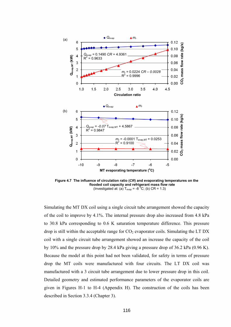
116

Figure 4.7 The influence of circulation ratio (CR) and evaporating temperatures on the

flooded coil capacity and refrigerant mass flow rate (Investigated at: (a) Tevap = -8 oC; (b) CR = 1.3)

Simulating the MT DX coil using a single circuit tube arrangement showed the capacity

of the coil to improve by 4.1%. The internal pressure drop also increased from 4.8 kPa

to 30.8 kPa corresponding to 0.6 K saturation temperature difference. This pressure

drop is still within the acceptable range for CO2 evaporator coils. Simulating the LT DX

coil with a single circuit tube arrangement showed an increase the capacity of the coil

by 10% and the pressure drop by 28.4 kPa giving a pressure drop of 36.2 kPa (0.96 K).

Because the model at this point had not been validated, for safety in terms of pressure

drop the MT coils were manufactured with four circuits. The LT DX coil was

manufactured with a 3 circuit tube arrangement due to lower pressure drop in this coil.

Detailed geometry and estimated performance parameters of the evaporator coils are

given in Figures H-1 to H-4 (Appendix H). The construction of the coils has been

described in Section 3.3.4 (Chapter 3).

CO

2 m

ass

flo

w r

ate

(kg

/s)

Qe

va

p,M

T (

kW)

Circulation ratio

Qevap mr

Qevap = 0.1490 CR + 4.9361R2 = 0.9633

mr = 0.0224 CR – 0.0028R2 = 0.9996

(a)

CO

2 m

ass

flo

w r

ate

(kg

/s)

MT evaporating temperature (oC)

Qe

va

p,M

T (

kW)

Qevap mr

Qevap = -0.07 Tevap,MT + 4.5867 R2 = 0.9847

mr = -0.0001 Tevap,MT + 0.0253 R2 = 0.9100

(b)

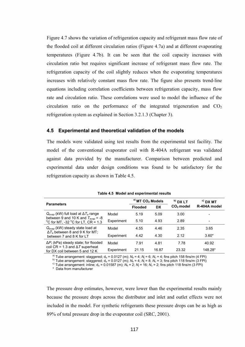
117

Figure 4.7 shows the variation of refrigeration capacity and refrigerant mass flow rate of

the flooded coil at different circulation ratios (Figure 4.7a) and at different evaporating

temperatures (Figure 4.7b). It can be seen that the coil capacity increases with

circulation ratio but requires significant increase of refrigerant mass flow rate. The

refrigeration capacity of the coil slightly reduces when the evaporating temperatures

increases with relatively constant mass flow rate. The figure also presents trend-line

equations including correlation coefficients between refrigeration capacity, mass flow

rate and circulation ratio. These correlations were used to model the influence of the

circulation ratio on the performance of the integrated trigeneration and CO2

refrigeration system as explained in Section 3.2.1.3 (Chapter 3).

44..55 EExxppeerriimmeennttaall aanndd tthheeoorreettiiccaall vvaalliiddaattiioonn ooff tthhee mmooddeellss

The models were validated using test results from the experimental test facility. The

model of the conventional evaporator coil with R-404A refrigerant was validated

against data provided by the manufacturer. Comparison between predicted and

experimental data under design conditions was found to be satisfactory for the

refrigeration capacity as shown in Table 4.5.

Table 4.5 Model and experimental results

Parameters a) MT CO2 Models b) DX LT

CO2 model

c) DX MT R-404A model Flooded DX

Qevap (kW) full load at ∆Ta range between 9 and 10 K and Tevap = -8 oC for MT, -32 oC for LT, CR = 1.3

Model 5.19 5.09 3.00 -

Experiment 5.10 4.93 2.89 -

Qevap (kW) steady state load at ∆Ta between 8 and 9 K for MT; between 7 and 8 K for LT

Model 4.55 4.46 2.35 3.65

Experiment 4.42 4.30 2.12 3.60*

∆Pr (kPa) steady state; for flooded coil CR = 1.3 and ∆T superheat for DX coil between 5 and 12 K

Model 7.91 4.81 7.78 40.92

Experiment 21.15 16.87 23.32 148.28*

a) Tube arrangement: staggered; do = 0.0127 (m); Nk = 4; Nj = 6; Nc = 4; fins pitch 158 fins/m (4 FPI) b) Tube arrangement: staggered; do = 0.0127 (m); Nk = 4; Nj = 8; Nc = 3; fins pitch 118 fins/m (3 FPI) c) Tube arrangement: inline; do = 0.01587 (m); Nk = 2; Nj = 16; Nc = 2; fins pitch 118 fins/m (3 FPI) * Data from manufacturer

The pressure drop estimates, however, were lower than the experimental results mainly

because the pressure drops across the distributor and inlet and outlet effects were not

included in the model. For synthetic refrigerants these pressure drops can be as high as

89% of total pressure drop in the evaporator coil (SRC, 2001).

118

44..66 PPeerrffoorrmmaannccee aannaallyysseess ooff CCOO22 eevvaappoorraattoorr ccooiillss

The validated models were used to design 8 evaporator coils with different geometry

and circuitry. The evaporator coils were simulated at evaporating temperature of -8 oC

for the MT coils and -30 oC for the LT coils. Tubes and fins were assumed to be made

of copper and aluminium respectively. Equilateral fin and tube pattern in a staggered

arrangement was assumed.

Table 4.6 Geometry of the designed coils and their performance parameters

Parameters MT evaporator coils LT evaporator coils

DX CO2 Flooded CO2 DX R-404A DX CO2 DX R-404A

EC-1 EC-2 EC-3 EC-4 EC-5 EC-6 EC-7 EC-8

do (mm) 9.52 12.70 9.52 12.70 15.87 9.52 12.70 15.87

Nk 2 2 2 2 2 2 2 2

Nj 21 17 13 10 20 12 10 12

Nc 2 1 2 1 2 2 1 2

Lt (m) 91.1 73.8 56.4 43.4 86.6 48.7 40.6 48.7

Lk (m) 0.064 0.064 0.064 0.064 0.076 0.064 0.064 0.076

Lj (m) 0.577 0.467 0.358 0.275 0.660 0.330 0.275 0.396

Li (m) 2.170 2.170 2.170 2.170 2.170 2.030 2.030 2.030

Vr (L) 4.14 6.78 2.56 3.99 13.47 2.22 3.74 7.57

Gr (kg/s.m2) 171.0 168.7 199.8 198.1 109.0 100.4 99.0 72.2

CR - - 1.2 1.2 - - - -

Qevap (kW) 3.75 3.75 3.75 3.76 3.76 2.25 2.25 2.25

Qevap,frost (kW)*

3.26 3.12 3.24 2.96 3.44 2.16 2.14 2.15

ηf** 0.85 0.88 0.85 0.88 0.87 0.89 0.92 0.90

hr (kW/m2.K) 2.899 3.107 3.206 3.473 0.482 2.521 2.802 0.337

ha (kW/m2.K) 0.062 0.073 0.064 0.075 0.063 0.042 0.050 0.046

∆Pr (kPa) 65.13 30.89 42.34 19.27 50.47 33.15 16.24 31.79

∆Pa,frost (kPa)* 0.016 0.024 0.030 0.043 0.013 0.018 0.020 0.010

* After frost accumulation of 4 (h) for MT coils and 48 (h) for LT coils;

** Fin thickness: 0.22 (mm) and fin pitch: 118 (fins/m); Vr is the refrigerant volume of the coils (litre).

Table 4.6 shows the geometry of the evaporator coils together with their performance

parameters. It can be seen that the physical sizes of the CO2 evaporator coils are much

smaller compared to the R-404A coils.

For the given refrigeration duty, the flooded MT coil with tube diameter 9.52 mm (EC-

3) has the smallest size with refrigerant volume about 62% of the MT DX coil with the

same tube diameter (EC-1) and about 19% of the refrigerant volume of the R-404A

evaporator coil (EC-5). The CO2 coils also need less refrigerant charge as shown in

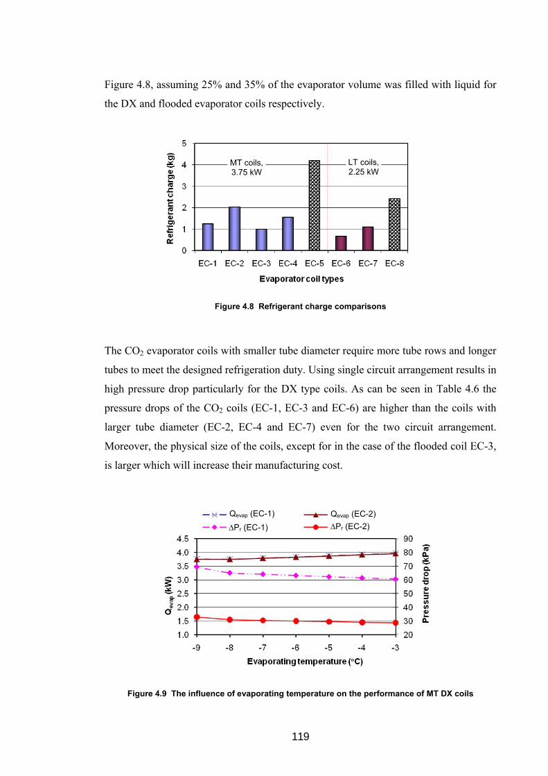
119

Figure 4.8, assuming 25% and 35% of the evaporator volume was filled with liquid for

the DX and flooded evaporator coils respectively.

Figure 4.8 Refrigerant charge comparisons

The CO2 evaporator coils with smaller tube diameter require more tube rows and longer

tubes to meet the designed refrigeration duty. Using single circuit arrangement results in

high pressure drop particularly for the DX type coils. As can be seen in Table 4.6 the

pressure drops of the CO2 coils (EC-1, EC-3 and EC-6) are higher than the coils with

larger tube diameter (EC-2, EC-4 and EC-7) even for the two circuit arrangement.

Moreover, the physical size of the coils, except for in the case of the flooded coil EC-3,

is larger which will increase their manufacturing cost.

Figure 4.9 The influence of evaporating temperature on the performance of MT DX coils

LT coils, 2.25 kW

MT coils, 3.75 kW

Qevap (EC-1) Qevap (EC-2)

∆Pr (EC-1) ∆Pr (EC-2)

120

Figure 4.9 shows the variation of the performance of CO2 MT DX coils with

evaporating temperature. Increasing the evaporating temperature can slightly improve

the refrigeration capacity and can reduce the pressure drop. This was also found to

apply to LT DX evaporator coils.

Figure 4.10 The influence of circulation ratio on the performance of the flooded coils

Figure 4.10 shows the performance of the flooded CO2 evaporator coils at different

circulation ratios (CR). As the CR increases, the refrigeration duty slightly improves due

to the enhancement of the evaporation heat transfer coefficient. However, the increase

of the CR considerably increases the pressure drop and refrigerant mass velocity which

increases the power consumption of the CO2 pump and causes a reduction in the

coefficient of performance of the refrigeration system. The CR, therefore, should be

chosen to be as low as possible in the range of the designed refrigeration capacity. The

mr (EC-4) mr (EC-3)

hr (EC-4) hr (EC-3) (b)

Qevap (EC-4) Qevap (EC-3)

∆Pr (EC-4) ∆Pr (EC-3) (a)

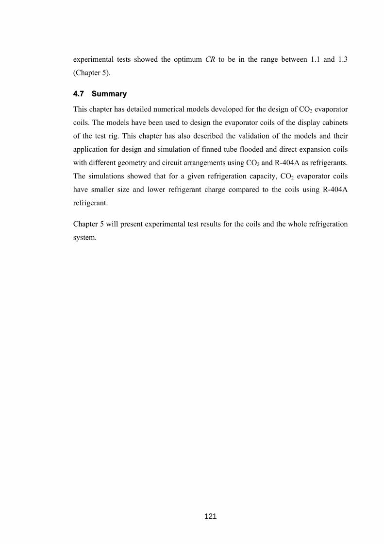
121

experimental tests showed the optimum CR to be in the range between 1.1 and 1.3

(Chapter 5).

44..77 SSuummmmaarryy

This chapter has detailed numerical models developed for the design of CO2 evaporator

coils. The models have been used to design the evaporator coils of the display cabinets

of the test rig. This chapter has also described the validation of the models and their

application for design and simulation of finned tube flooded and direct expansion coils

with different geometry and circuit arrangements using CO2 and R-404A as refrigerants.

The simulations showed that for a given refrigeration capacity, CO2 evaporator coils

have smaller size and lower refrigerant charge compared to the coils using R-404A

refrigerant.

Chapter 5 will present experimental test results for the coils and the whole refrigeration

system.

122

CChhaapptteerr 55

EEXXPPEERRIIMMEENNTTAALL TTEESSTT RREESSUULLTTSS AANNDD MMOODDEELL VVAALLIIDDAATTIIOONN

This chapter reviews the as-built test facility and reports experimental test results on the

performance of volatile medium temperature (MT) CO2 refrigeration with different

circulation ratios and different evaporating temperatures. The performance of low

temperature (LT) direct expansion refrigeration as well as the combined MT and LT

performance is also considered. This chapter also briefly describes the test conditions

and procedure, parameter setting, data collection and processing which includes

uncertainty analyses of the test results. Validation of the simulation models is also

presented.

55..11 OOvveerrvviieeww ooff tthhee aass--bbuuiilltt tteesstt ffaacciilliittyy

The test facility consists of three main modules: CHP module, absorption refrigeration

module and retail refrigeration system module as shown in Figure 5.1. The CHP module

is based on an 80 kWe recuperated micro gas turbine generation package with in-built

boiler heat exchanger (exhaust heat recovery heat exchanger). The 3-phase electrical

power output from the high speed alternator can be modulated in the range 30 kWe to 80

kWe.

The absorption refrigeration module currently employed is based on a packaged direct

gas fired ROBUR chiller which has been re-engineered to operate with a heat transfer

fluid heated by the exhaust gases of the microturbine in the CHP module. The

123

absorption module was integrated with the CHP module through the in-built boiler heat

exchanger and heat transfer fluid (HTF) system (Figure 5.1) to form the trigeneration

system.

The capacity of the installed absorption module is about 30% of the possible optimum

capacity of the trigeneration system. The refrigeration capacity of the trigeneration

system is dependent on the type of thermally driven refrigeration system used. For

ammonia-water refrigeration systems providing refrigeration to -10 oC, the trigeneration

system can provide up to 30 kW of refrigeration which recovers approximately 50 kW

wasted heat of the CHP module. To achieve this, a new indirectly heated generator was

developed and implemented on the absorption chiller. Further performance

improvement could be achieved through better integration of the CHP system and

absorption chiller to reduce pumping power and pipe heat losses.

Figure 5.1 Simplified diagram of the integrated volatile-DX CO2 refrigeration and trigeneration (Detailed diagram of the integrated system is shown in Figure I-1; Appendix I)

The retail refrigeration system module as shown in Figure 5.2 consists of a cascade

volatile MT and direct expansion LT CO2 refrigeration system and associated test

facilities which include an environmental test chamber and chilled and frozen food

Chilled fluid pump

Absorption refrigeration module

Exhaust gas

CHP module

MT Display cabinet

LT Display cabinet

CO2 CompressorBock HGX12P/60-4 CO2 CO2 Pump

CO2 liquid receiver

IHX

CO2 condenser

Air

Fuel

Electricity

Boiler HX

Generator set

Hot fluid pump

RV

Byp

ass

valv

e

PRV

Retail refrigeration system module

Trigeneration system

Robur ACF 60-00 LB

124

display cabinets located in the chamber to provide controlled load to the refrigeration

system. The refrigerated display cabinets, chilled open vertical multi-deck, and glass

door frozen food which were originally designed with R-404A refrigerant were

modified by replacing the evaporator coil and controls, to operate with CO2 refrigerant.

The evaporator coil of the low temperature cabinet is a direct expansion coil whereas

the coil of the medium temperature cabinet is a flooded evaporator coil which is

designed to operate with CO2 as a secondary (volatile) refrigerant. Condensation of the

CO2 from both the low and medium temperature sections of the system is provided by

the absorption refrigeration system of the trigeneration facility through a CO2 condenser

in the form of a plate heat exchanger. The CO2 condenser is installed just above the

liquid receiver to facilitate the flow of liquid CO2 from the condenser by gravity. The

system was designed so that the CO2 for the medium temperature cabinet could be

either pumped with a centrifugal CO2 pump or gravity fed to the coil.

Figure 5.2 Retail refrigeration system module with CO2 refrigeration system

The test facility is equipped with Danfoss controllers and was comprehensively

instrumented with power metres, pressure transducers, thermocouples, relative humidity

sensors and coriolis refrigerant flow meters to enable detailed investigations of the

transient and steady state performance of individual components and the overall system.

Monitoring is performed through a data logging system which can scan and store the

measured parameters at present time intervals.

(a) CO2 pump and compressor section

(b) CO2 condenser and liquid receiver section

(c) MT and LT loading system

125

55..22 EExxppeerriimmeennttaall tteesstt ccoonnddiittiioonnss aanndd ddaattaa pprroocceessssiinngg

A series of tests was carried out to evaluate energy performance of the CO2 refrigeration

system which comprised performance of the MT and LT system as well as that of the

overall CO2 refrigeration system. Tests were performed with different circulation ratios

(CR) and different evaporating temperatures for the MT CO2 refrigeration system.

System performance parameters were recorded and used to determine the refrigeration

capacity and coefficient of performance (COP) of the LT, MT and overall CO2

refrigeration system.

5.2.1 Test conditions

The tests on the MT refrigeration system were carried out at three evaporating

temperature levels: -6 oC, -8 oC and -10 oC. Each temperature level was tested at

different refrigerant mass flow rates or circulation ratios. Tests on the LT circuit and

overall system were carried out at circulation ratio CR = 1.3, condensing and

evaporating temperatures at Tcond = -7 oC and Tevap,LT = -32 oC respectively.

The chilled and frozen food display cabinets were placed in the test room as described

in Section 3.8 (Chapter 3). The test chamber was conditioned at climate class 3 (25°C

and 60% RH). These conditions were measured at a point in the middle of the MT

display cabinet 150 mm above and 300 mm in front of the top edge of the cabinet

opening. The display cabinets including the product packages and temperature

measurement points have been explained in Section 3.4.1 (Chapter 3). On the air side of

the MT display cabinet, besides temperatures, the relative humidity (RH) of the air-on

and air-off the coil was also measured and recorded. The MT and LT cabinets were

tested for M1 and L1 classification respectively. An M1 cabinet requires product

temperatures ranging from -1 oC to +5 oC and a cabinet of L1 classification requires the

highest temperature of the warmest product to be lower or equal to -15 oC and the

lowest temperature of this warmest product to be lower or equal to -18 oC (ISO 23953-

2, 2005).

5.2.2 Experimental test procedure

The test facility was operated according to the mode of tests and following the

operational procedure as detailed in Appendix G. In order to investigate the transient

performance, the system was monitored from start up to the point it achieved steady

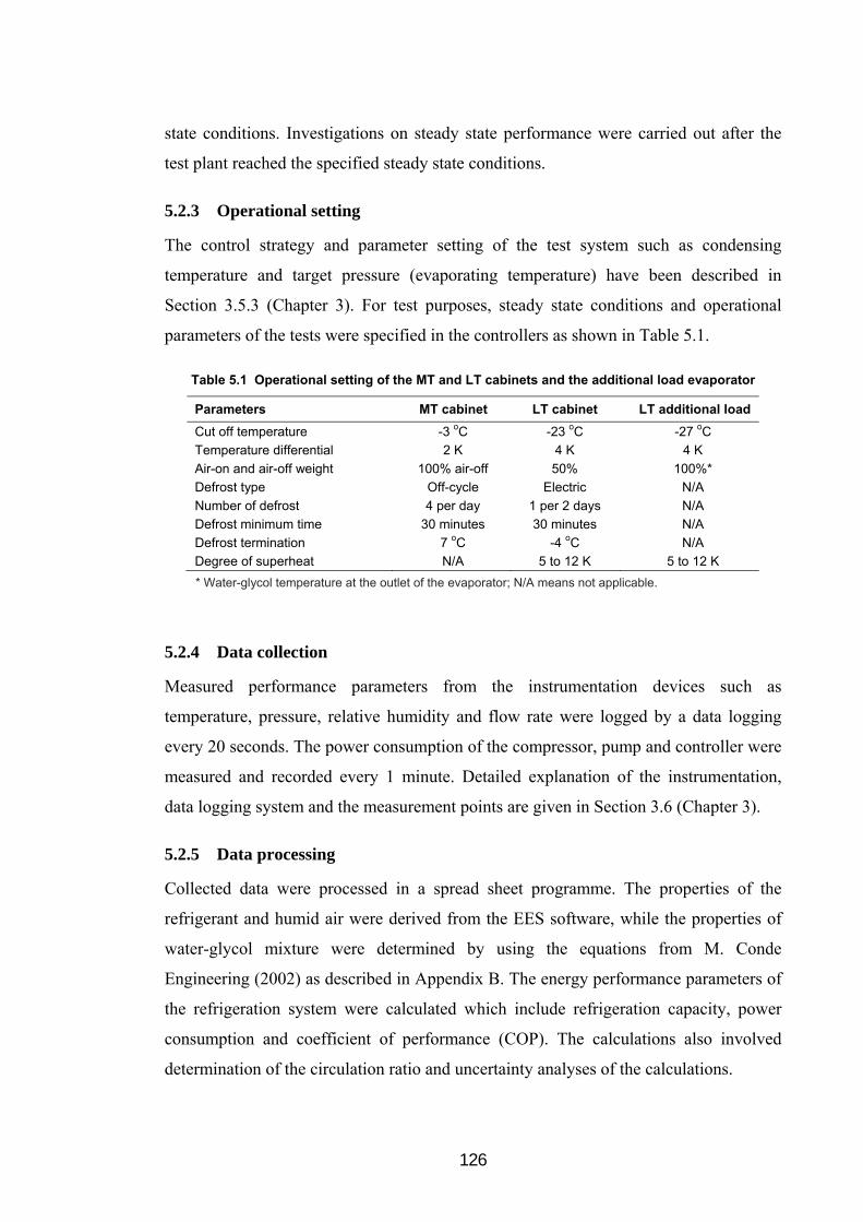
126

state conditions. Investigations on steady state performance were carried out after the

test plant reached the specified steady state conditions.

5.2.3 Operational setting

The control strategy and parameter setting of the test system such as condensing

temperature and target pressure (evaporating temperature) have been described in

Section 3.5.3 (Chapter 3). For test purposes, steady state conditions and operational

parameters of the tests were specified in the controllers as shown in Table 5.1.

Table 5.1 Operational setting of the MT and LT cabinets and the additional load evaporator

Parameters MT cabinet LT cabinet LT additional load

Cut off temperature -3 oC -23 oC -27 oC

Temperature differential 2 K 4 K 4 K

Air-on and air-off weight 100% air-off 50% 100%*

Defrost type Off-cycle Electric N/A

Number of defrost 4 per day 1 per 2 days N/A

Defrost minimum time 30 minutes 30 minutes N/A

Defrost termination 7 oC -4 oC N/A

Degree of superheat N/A 5 to 12 K 5 to 12 K

* Water-glycol temperature at the outlet of the evaporator; N/A means not applicable.

5.2.4 Data collection

Measured performance parameters from the instrumentation devices such as

temperature, pressure, relative humidity and flow rate were logged by a data logging

every 20 seconds. The power consumption of the compressor, pump and controller were

measured and recorded every 1 minute. Detailed explanation of the instrumentation,

data logging system and the measurement points are given in Section 3.6 (Chapter 3).

5.2.5 Data processing

Collected data were processed in a spread sheet programme. The properties of the

refrigerant and humid air were derived from the EES software, while the properties of

water-glycol mixture were determined by using the equations from M. Conde

Engineering (2002) as described in Appendix B. The energy performance parameters of

the refrigeration system were calculated which include refrigeration capacity, power

consumption and coefficient of performance (COP). The calculations also involved

determination of the circulation ratio and uncertainty analyses of the calculations.

127

5.2.5.1 Calculation of the refrigeration capacity

The refrigeration capacity of the evaporators of the display cabinets was calculated

using the enthalpy difference across the coil and the mass flow rate of refrigerant. For

the LT DX evaporator the expansion of the refrigerant was assumed to be isenthalpic.

The enthalpy of the refrigerant liquid entering the evaporator, Hr,i,LT , and the refrigerant

vapour leaving the evaporator, Hr,o,LT , were determined from measurements of

temperature and pressure of the refrigerant at inlet of the expansion valve and outlet of

the evaporator respectively. For the MT flooded evaporator, the enthalpy of the

refrigerant entering the evaporator, Hr,i,MT , was determined from the MT evaporating

temperature and pressure, while the enthalpy of the refrigerant leaving the evaporator,

Hr,o,MT , was determined from the evaporating temperature and vapour quality of the

refrigerant at the outlet of the evaporator (xo), where xo = 1/CR. The calculation of the

circulation ratio (CR) is detailed in Section 5.2.5.4. For the LT DX additional load, the

refrigeration capacity was calculated from the energy balance between the refrigerant

and the water-glycol sides assuming adiabatic heat transfer. The refrigeration capacities

of the MT and LT systems were calculated from:

)( ,,,,, MTirMTorMTrMT HHmQ (5.1)

addLTcabLTLT QQQ ,, (5.2)

where:

)( ,,,,,, LTirLTorLTrcabLT HHmQ (5.3)

)( ,,,, owiwwpwaddLT TTCmQ (5.4)

QLT,cab and QLT,add are the refrigeration capacities of the evaporator of the frozen food

display cabinet and additional load respectively; wm is the water-glycol mass flow rate.

5.2.5.2 Power consumption

The total power consumption of the system is the sum of the power consumption of the

LT compressor and the power consumption of the CO2 pump. The power consumption

of the LT compressor (Wcomp) was determined by recording the power when only the LT

system was in operation, whereas the power consumption of the CO2 pump was

128

determined when only the MT system was in operation. Because the refrigerant flow

rate from the pump was partially bypassed to the liquid receiver, the pumping power

(WCO2,pump) used in the COP calculation was assumed to be proportional to the measured

refrigerant mass flow rate through the MT evaporator coil.

5.2.5.3 Calculation of the COP

The coefficient of performance (COP) of the LT, MT and overall refrigeration system

were calculated from the equations described in Chapter 3: (3.15), (3.16) and (3.17)

respectively. The COP of the LT system was also compared to the reversed Carnot

cycle calculated from:

LTevapLTcond

LTevapCarnot TT

TCOP

,,

,

(5.5)

where evaporating and condensing temperatures Tevap,LT and Tcond,LT respectively are in

Kelvin (K).

5.2.5.4 Circulation ratio

The flow of CO2 refrigerant in the MT evaporator coil starts as liquid, gradually

evaporates along the coil pipe and then exits the evaporator coil at certain quality (xo)

which is the inverse value of the circulation ratio (CR). The circulation ratio, as defined

in Section 3.2.1.3 (Chapter 3) can be determined from:

vap

MTr

m

mCR

, (5.6)

where MTrm , = total refrigerant mass flow rate in MT evaporator, vapm = refrigerant

vapour mass flow rate, and CR = 1 occurs when vapMTr mm , .

In the test system, CR = 1 can be established by adjusting the regulator and bypass

valves upstream of the MT evaporator coil while observing the quality of the liquid

refrigerant flowing through a sight glass fitted at the outlet of the coil. In order to make

the adjustment of the refrigerant flow rate easier, the regulator valve should be installed

adjacent to the sight glass as shown in Figure 5.1 and the adjustment should be started

from overfeed flow rate so that the liquid refrigerant can be clearly seen in the sight

129

glass. With the bypass valve slightly open, the regulator valve can be gradually closed

until the liquid refrigerant just disappears from the sight glass. The supplied mass flow

rate to the evaporator ( MTrm , ), can then be measured from the flow meter which is fitted

on the liquid line upstream of the MT evaporator coil. The mass flow of refrigerant

vapour ( vapm ) at a particular evaporating temperature (Tevap,MT) can be calculated from:

fg

MTvap H

Qm (5.7)

where Hfg is the enthalpy of evaporation of the CO2 refrigerant at evaporating

temperature (Tevap,MT). QMT is the refrigeration load of the MT cabinet which is

equivalent to the heat absorbed from the air crossing the MT coil and can be determined

from:

)( ,, OFFaONaaMT HHmQ (5.8)

am is the mass flow rate of the air flowing through the evaporator coil as a function of

air velocity and cross sectional area of the air passage in the cabinet; Ha,ON and Ha,OFF

are the enthalpies of the air entering and leaving the coil respectively.

In a real supermarket application, the circulation ratio can be controlled by integrating

the cabinet controller with a motorized valve installed upstream of the evaporator coil

and with the speed controller of the CO2 pump.

5.2.5.5 Uncertainty in the calculation of CR and COP

Considering the uncertainty of the measured variables which include air mass flow rate,

air temperature and relative humidity, refrigerant temperatures, pressures, power and

refrigerant mass flowrate and assuming that the individual measurements are

uncorrelated and random, the uncertainty in the calculation of CR was determined, using

the Engineering Equation Solver (EES) software, to be ± 10.8%. The uncertainty in the

calculations of the COPLT, COPMT, COPOverall and COPCarnot were found to be ± 0.2%

± 10.8%, ± 3.6% and ± 0.6% respectively. The uncertainty of the COPMT is relatively

high because its calculation involved the circulation ratio. Detailed explanation of the

uncertainty analysis is given in Appendix J.

130

55..33 TTeesstt rreessuullttss

5.3.1 Thermodynamic cycle of the refrigeration system

Figure 5.3 shows the thermodynamic cycle of the CO2 refrigeration system obtained

from the test results. The cycle refers to the schematic diagram Figure 3.4 (Chapter 3).

Pressure drop of MT circuit (9-10-11) was found to be 37.5 kPa which corresponds to

0.5 K temperature drop. The pumping process (9-10) and heat extraction process in the

MT cabinet (10-11) can be assumed to be at constant temperature and pressure.

Figure 5.3 Pressure-enthalpy diagram of the CO2 refrigeration cycle based on the test results

Figure 5.3 also shows the LT circuit (1-2-3-4-5-6-7-8) which was integrated with the

heat rejection loop of the MT system (12-3-4). The circuit was equipped with an

internal heat exchanger (IHX) which exchanged heat from cold stream (8-1) to the hot

stream (5-6) of the circuit to provide sub-cooling of around 2.5 K on the CO2 liquid

before being expanded into liquid-vapour mixture through the EXV. This exchanged

heat increased the superheat of the CO2 gas from the LT evaporator (of 5 K

superheating at point 8) to be around 10 K superheating (at point 1) before entering the

LT compressor. The expansion process in the EXV (6-7) was assumed to be isenthalpic.

The compression process (1-2) utilised a semi hermetic reciprocating compressor of

isentropic efficiency of around 0.69. This efficiency is discussed further in Section 5.4.

Pressure (kPa) is absolute pressure

Enthalpy (kJ/kg)

-32oC

-7oC

8oC

Pre

ssu

re (

kPa

)

0.2 0.4 0.6 0.8

64,5,9

10

11

12 3 2

1

8

7

-500 -400 -300 -200 -100 0 100 500

1000

10000

20000

42oCR-744

2870

1350

∆Tsc = 2.5 K

∆Tsh = 10 K

131

5.3.2 Medium temperature refrigeration system

For the MT CO2 refrigeration system, investigations were carried out to establish the

impact of the circulation ratio on the performance of the coil and the MT CO2

refrigeration system at different evaporating temperatures. The results showed that the

MT system can achieve very high COPs ranging from 32 to 60, due to the low power

consumption of the CO2 pump.

Figure 5.4 Variation of MT refrigeration capacity and COP with circulation ratio for different evaporating temperatures

The COP and refrigeration capacity of the MT refrigeration system vary with circulation

ratio and the evaporating temperature as shown in Figure 5.4. Increasing the circulation

ratio increases the refrigeration capacity, reaching a maximum at a circulation ratio of

1.3. Because of the increase in pumping power with increasing refrigerant flow rate,

(a) MT refrigeration capacity (b) COP of the MT system

Circulation ratio

CO

PM

T

Tevap = -6 oC

Tevap = -8 oC

Tevap = -10 oC

(b)

wet dry

Circulation ratio

QM

T

(a)

Tevap = -6 oC

Tevap = -8 oC

Tevap = -10 oC

wet dry

132

however, the increase in the circulation ratio causes a reduction in the system COP. For

the system tested, the optimum CR was found to be in the range between 1.1 and 1.3.

Figure 5.4 also shows that at constant circulation ratio, the COP slightly increases as the

evaporating temperature decreases. This is contrary to what is expected for a direct

expansion refrigeration system and can be explained as follows: in a flooded evaporator,

reducing the evaporation temperature can improve heat transfer due to the higher

temperature difference between the refrigerant and the air. This will enhance the

evaporation rate of the refrigerant in the coil which in turn will increase the vapour

quality at the exit of the evaporator coil, causing a reduction in the circulation ratio. In

order to maintain a constant CR, the mass flowrate of refrigerant will have to be

increased. This will improve further the heat transfer of the CO2 refrigerant and will

also increase the refrigeration capacity of the evaporator coil which leads to a higher

COP. These results are in agreement with the results from the flooded evaporator model

which have been explained in Section 4.4 (Figure 4.7). For a DX refrigeration system,

on the other hand, the refrigeration capacity will decrease when the evaporating

temperature reduces. This has been described in Section 4.6 (Chapter 4).

Figure 5.5 Performance of the CO2 MT refrigeration system (Investigated at evaporating temperatures of -7 oC and CR = 1.3)

The performance of the MT CO2 refrigeration system with time at circulation ratio CR =

1.3 and evaporating temperature -7 oC is shown in Figure 5.5. From the figure it can be

seen that the MT system consumes very low pump power of 0.110 kW in average. The

COP of the MT system which was calculated as the ratio of the cooling done by the

df Reaching set point df

Time (minutes)

WC

O2p

um

p a

nd

QM

T (

kW)

CO

PM

T

QMT

COPMT

Wpump

df = defrost

133

evaporator coil to the pump power consumption was around 45.4. The MT system

delivers an average refrigeration capacity of 4.9 kW.

Figure 5.5 also shows the pump cycling off in response to: i) the cabinet coil air-off

temperature which was set at -3 oC and; ii) during the defrost cycle. For the MT system,

the off-cycle defrost control was set at 4 defrost cycles per 24 hour period. Defrost

termination was controlled on coil air-off temperature of 7 oC or elapsed time of 30

minutes whichever was reached first.

5.3.3 Low temperature refrigeration system

Figure 5.6 shows performance of the LT CO2 refrigeration system with time at

condensing temperature -7 oC and evaporating temperature -32 oC. It can be seen that

the LT system can deliver a steady state COP of 4.0 with refrigeration capacity (QLT) of

about 10 kW.

Figure 5.6 also shows the compressor cycling off when the air temperature in the

cabinet reaches the set point. Defrost cycle of the LT cabinet, however, could not be

seen within this test period because the electric defrost of the cabinet was set for 30

minutes every 48 hours. These defrost control settings were found to be satisfactory for

the conditions tested.

Figure 5.6 Performance of the CO2 LT refrigeration system (Investigated at condensing and evaporating temperatures of -7 oC and -32 oC)

The variation of evaporating and condensing temperatures of the LT system is shown in

Figure 5.7. The evaporating temperature was measured at inlet to the LT evaporator just

after the expansion valve, while the condensing temperature was measured at the outlet

Time (minutes)

Wco

mp a

nd

QL

T (

kW)

CO

P

QLT

COPLT Wcomp

134

of the condenser. The average evaporating and condensing temperatures were -32 oC

and -7 oC respectively with average measured pressures of 12.5 bar and 27.7 bar.

Figure 5.7 also shows the average reversed Carnot COP of the LT system to be around

9.6. The actual COP is less than half of the Carnot COP due to irreversibilities of

expansion and compression processes in the actual cycle as well as electrical,

mechanical and volume losses from the compressor.

Figure 5.7 Evaporation and condensing temperatures including theoretical COP of the LT system

5.3.4 Overall refrigeration system

Figure 5.8 shows the performance of the MT and LT refrigeration systems and the

combined performance of the MT and LT circuits at an evaporating temperature of -7 oC for the MT system and -32 oC for the LT system and a circulation ratio for the

refrigerant in the MT evaporator coil of 1.3.

From Figure 5.8 it can also be seen that the average overall COP of the CO2

refrigeration system, MT and LT, varied in the range between 5.5 and 6. The total

refrigeration load for the system was 15 kW of which 5 kW was for the MT system and

10 kW for the LT system. In supermarkets the LT load is normally between 20% and

30% of the MT load but in the experimental facility the balance of load for the MT and

LT systems was decided by the availability of compressors at the time the facility was

constructed. A change in the load balance between the LT and MT to better reflect the

actual load balance in a supermarket would have resulted in an even higher overall COP

for the system.

Tevap,in

Tcond,out

COPCarnot

Time (minutes)

Tem

per

atu

re (

oC

)

CO

PC

arn

ot

135

Figure 5.8 Performance of the CO2 MT and LT refrigeration systems

5.3.5 Product and air temperatures

Product and air temperatures of the MT and LT cabinets were used as a measure of

establishing whether the CO2 refrigeration system had reached steady state condition.

When the product temperatures of the MT and LT cabinet were relatively stable in the

range M1 and L1 temperature classifications (as specified in Section 5.2.1) respectively,

the MT and LT systems were considered to have reached steady state conditions. These

conditions were used for the analysis of the CO2 refrigeration cycle performance as

described in the previous sections.

Figure 5.9 Variation of the MT product temperatures with time (Investigated at circulation ratio of 1.3 and evaporating temperatures of -7 oC)

Investigated at circulation ratio of 1.3, condensing and evaporating temperatures of -7 oC and -32 oC; df = defrost

Steady state conditions

MT and LT systems reaching the set points

Defrost effect

Defrost effect

df Reaching MT set point df

COPLT

COPoverall

COPMT

Time (minutes)

CO

PM

T

CO

PL

T a

nd

CO

Po

ve

rall

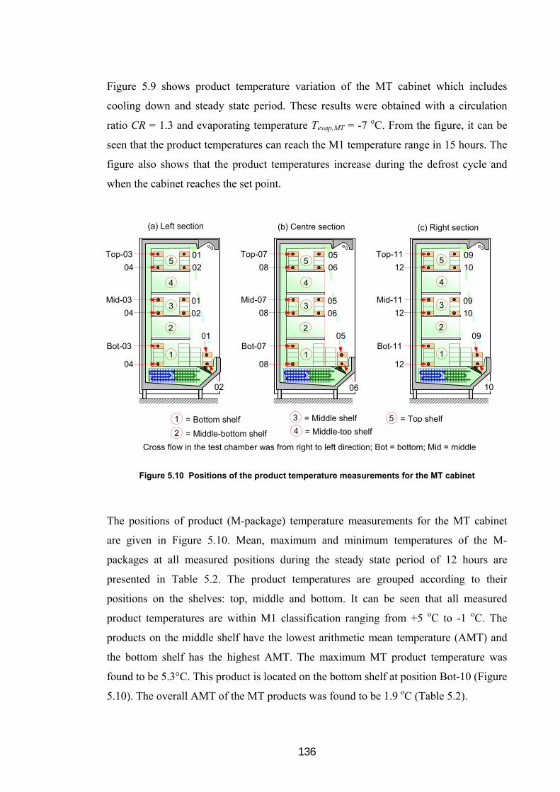
136

Figure 5.9 shows product temperature variation of the MT cabinet which includes

cooling down and steady state period. These results were obtained with a circulation

ratio CR = 1.3 and evaporating temperature Tevap,MT = -7 oC. From the figure, it can be

seen that the product temperatures can reach the M1 temperature range in 15 hours. The

figure also shows that the product temperatures increase during the defrost cycle and

when the cabinet reaches the set point.

Figure 5.10 Positions of the product temperature measurements for the MT cabinet

The positions of product (M-package) temperature measurements for the MT cabinet

are given in Figure 5.10. Mean, maximum and minimum temperatures of the M-

packages at all measured positions during the steady state period of 12 hours are

presented in Table 5.2. The product temperatures are grouped according to their

positions on the shelves: top, middle and bottom. It can be seen that all measured

product temperatures are within M1 classification ranging from +5 oC to -1 oC. The

products on the middle shelf have the lowest arithmetic mean temperature (AMT) and

the bottom shelf has the highest AMT. The maximum MT product temperature was

found to be 5.3°C. This product is located on the bottom shelf at position Bot-10 (Figure

5.10). The overall AMT of the MT products was found to be 1.9 oC (Table 5.2).

(a) Left section

01

02

04

Bot-03

04

Mid-03

04

Top-03

02

01

02

01

1

2

3

4

5

(b) Centre section

05

06

08

Bot-07

08

Mid-07

08

Top-07

06

05

06

05

(c) Right section

09

10

12

Bot-11

12

Mid-11

12

Top-11

10

09

10

09

= Bottom shelf1

= Middle-bottom shelf2

= Middle shelf3

= Middle-top shelf4

= Top shelf 5

Cross flow in the test chamber was from right to left direction; Bot = bottom; Mid = middle

1

2

3

4

5

1

2

3

4

5

137

Table 5.2 Mean, maximum and minimum temperatures of the MT products

Measured positions

Max. Min. Mean Measured positions

Max. Min. Mean Measured positions

Max. Min. Mean

Top-01 3.8 1.8 2.9 Mid-01 2.1 0.5 1.2 Bot-01 2.1 1.0 1.6

Top-02 3.7 1.8 2.8 Mid-02 2.3 0.8 1.5 Bot-02 2.8 1.8 2.3

Top-03 0.1 -1.4 -0.5 Mid-03 -0.4 -1.3 -0.9 Bot-03 -0.2 -1.2 -0.7

Top-04 1.0 -1.2 -0.1 Mid-04 0.0 -1.2 -0.5 Bot-04 2.0 0.6 1.3

Top-05 4.7 2.7 3.9 Mid-05 4.1 2.7 3.5 Bot-05 2.9 1.6 2.3

Top-06 4.4 2.8 3.6 Mid-06 3.4 2.1 2.8 Bot-06 4.8 3.4 4.2

Top-07 0.3 -0.8 0.1 Mid-07 0.5 -1.1 -0.2 Bot-07 1.8 0.7 1.3

Top-08 0.8 -0.8 0.0 Mid-08 0.6 -0.8 -0.1 Bot-08 4.0 2.7 3.4

Top-09 5.1 3.6 4.5 Mid-09 4.1 2.9 3.6 Bot-09 4.5 3.4 4.0

Top-10 4.4 3.1 3.8 Mid-10 2.8 1.6 2.2 Bot-10 5.3 4.0 4.7

Top-11 5.0 0.4 2.4 Mid-11 1.6 0.1 0.8 Bot-11 2.5 1.2 1.9

Top-12 1.4 0.5 1.0 Mid-12 1.0 -0.2 0.4 Bot-12 4.0 2.8 3.3

AMT of the top shelf 2.0 AMT of the middle shelf 1.2 AMT of the bottom shelf 2.5

AMT overall of the MT products 1.9

AMT = average mean temperature; Bot = bottom shelf; Mid = middle shelf; Top = top shelf; Max. = maximum temperature; Min. = minimum temperature. Measured positions of the MT products refer to Figure 5.10

Figure 5.11 Variation of air temperatures and RHs of the MT cabinet

Variations for air temperature entering the MT evaporator coil (air-on) and leaving the

coil (air-off) are shown in Figure 5.11. The temperatures are average of three point

measurements measured at the right, centre and left hand side of the air passage of the

MT cabinet before and after the evaporator coil. It can be seen that the air temperatures

vary periodically during the test due to the defrost cycle. The temperature difference

Frost accumulation showed effect to the ∆Tair

in the last 2 hours of defrost cycles

138

between the air-on and air-off is approximately 10 oC after start up and just after defrost.

The temperature difference starts to increase after 4 hours from defrost and reaches

more than 12 oC just before the next defrost cycle.

Figure 5.11 also shows the variation of relative humidity (RH) at evaporator coil air-on

and air-off measured at the centre section of the MT cabinet. It can be seen that the

relative humidity of the air-on and off tends to equalise during the defrost cycle when

refrigerant is not flowing through the coil. During the cooling cycle the difference

between the RH value on and off the coil tends to increase with frost accumulation on

the coil and reaches maximum just before defrost.

Figure 5.12 Variation of the LT product temperatures with time (Investigated at condensing and evaporating temperatures of -7 oC and -32 oC respectively)

Figure 5.12 shows the variation of the product temperatures of the LT cabinet. The

results were obtained at evaporating and condensing temperatures -32 oC and -7 oC

respectively and with the doors of the cabinet closed. The temperatures reached the L1

temperature classification (below -15 oC) in 15 hours. At a stable condition, the

difference between the maximum and minimum product temperatures was about 5 oC.

Figure 5.12 also shows the super-cooling behaviour of the M-packages when their

temperatures first dropped below their freezing point of -1 oC.

Positions of the measured product (M-packages) for the LT cabinet are shown in Figure

5.13. Detailed results of the LT product temperature measurements which include

Steady state conditions

Super-cooling temperature of the

M-packages

AMT overall = -20.7 oC Highest temperature of the

warmest M-package = -15.7 oC Lowest temperature of the

warmest M-package = -20.1 oC

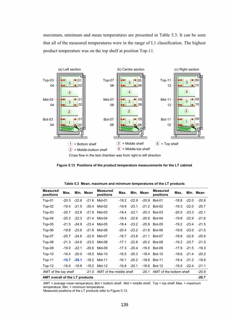
139

maximum, minimum and mean temperatures are presented in Table 5.3. It can be seen

that all of the measured temperatures were in the range of L1 classification. The highest

product temperature was on the top shelf at position Top-11.

Figure 5.13 Positions of the product temperature measurements for the LT cabinet

Table 5.3 Mean, maximum and minimum temperatures of the LT products

Measured positions

Max. Min. Mean Measured positions

Max. Min. Mean Measured positions

Max. Min. Mean

Top-01 -20.3 -22.6 -21.6 Mid-01 -19.2 -22.9 -20.9 Bot-01 -18.8 -22.0 -20.8

Top-02 -19.4 -21.5 -20.4 Mid-02 -19.9 -23.1 -21.2 Bot-02 -19.3 -22.0 -20.7

Top-03 -20.7 -22.8 -21.9 Mid-03 -18.4 -22.1 -20.3 Bot-03 -20.5 -23.3 -22.1

Top-04 -20.3 -22.3 -21.4 Mid-04 -18.4 -22.6 -20.6 Bot-04 -19.8 -22.9 -21.6

Top-05 -21.5 -24.9 -23.4 Mid-05 -18.4 -23.2 -20.9 Bot-05 -19.2 -23.4 -21.5

Top-06 -19.8 -23.6 -21.8 Mid-06 -20.4 -23.2 -21.8 Bot-06 -19.6 -23.0 -21.5

Top-07 -20.7 -24.6 -22.9 Mid-07 -18.7 -23.6 -21.1 Bot-07 -18.8 -22.6 -20.6

Top-08 -21.3 -24.6 -23.0 Mid-08 -17.1 -22.8 -20.2 Bot-08 -19.2 -23.7 -21.5

Top-09 -19.0 -22.1 -20.6 Mid-09 -17.3 -20.4 -19.0 Bot-09 -17.9 -21.5 -19.3

Top-10 -16.4 -20.0 -18.5 Mid-10 -16.5 -20.3 -18.4 Bot-10 -18.6 -21.4 -20.2

Top-11 -15.7 -20.1 -18.2 Mid-11 -16.1 -20.2 -18.6 Bot-11 -18.4 -21.2 -19.9

Top-12 -16.0 -19.8 -18.2 Mid-12 -16.8 -20.1 -18.6 Bot-12 -19.5 -22.4 -21.1

AMT of the top shelf -21.0 AMT of the middle shelf -20.1 AMT of the bottom shelf -20.9

AMT overall of the LT products -20.7

AMT = average mean temperature; Bot = bottom shelf; Mid = middle shelf; Top = top shelf; Max. = maximum temperature; Min. = minimum temperature. Measured positions of the LT products refer to Figure 5.13.

(a) Left section

 

1

2

3

4

5 04

Top-03

04

Mid-03

04

Bot-03

= Bottom shelf1

= Middle-bottom shelf2

= Middle shelf3

= Middle-top shelf4

= Top shelf 5

Cross flow in the test chamber was from right to left direction

(b) Centre section

 

08

Top-07

08

Mid-07

08

Bot-07

(c) Right section

 

12

Top-11

12

Mid-11

12

Bot-11 05

06

06

05

06

05

1

2

3

4

5

1

2

3

4

5

09

10

10

09

10

09

01

02

02

01

02

01

140

Figure 5.14 shows the temperature variation of the air-on and air-off the LT evaporator

coil. These temperatures were the averages of three measurements on the right, centre

and left sections of the LT cabinet before and after the evaporator coil. The fluctuations

in the temperatures that can be observed are due to the closure of the expansion valve

which switched the flow of refrigerant off when the cabinet set point temperature was

reached. At steady state conditions the difference in temperature between air-on and air-

off the coil was around 8 oC. The figure also presents the variation of the relative

humidity on and off the coil measured at the centre section of the LT cabinet. During

steady state conditions, the difference between the air-on and air-off relative humidity

was approximately 25%.

Figure 5.14 Variation of air temperatures and RHs of the LT cabinet

5.3.6 Frost performance of the CO2 display cabinets

Excessive frost on the surface of the evaporator coil will reduce the air circulation in the

cabinet and cause an increase in the product temperature especially in the case of the

MT cabinet as previously described. Figure 5.15 shows the accumulation of frost on the

surface of the MT evaporator coil after 4 hours from defrost. It can be seen that frost

accumulation was fairly uniform across the coil surface.

The amount of frost accumulated on the surface of the MT evaporator coil was

measured by collecting the drained water from the cabinet during the defrost cycle. The

results are shown in Figure 5.16a. These measurements were taken at different

Steady state conditions

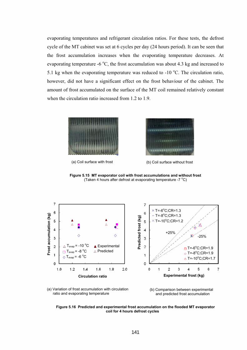
141

evaporating temperatures and refrigerant circulation ratios. For these tests, the defrost

cycle of the MT cabinet was set at 6 cycles per day (24 hours period). It can be seen that

the frost accumulation increases when the evaporating temperature decreases. At

evaporating temperature -6 oC, the frost accumulation was about 4.3 kg and increased to

5.1 kg when the evaporating temperature was reduced to -10 oC. The circulation ratio,

however, did not have a significant effect on the frost behaviour of the cabinet. The

amount of frost accumulated on the surface of the MT coil remained relatively constant

when the circulation ratio increased from 1.2 to 1.9.

Figure 5.15 MT evaporator coil with frost accumulations and without frost

(Taken 4 hours after defrost at evaporating temperature -7 oC)

Figure 5.16 Predicted and experimental frost accumulation on the flooded MT evaporator coil for 4 hours defrost cycles

(a) Coil surface with frost (b) Coil surface without frost

Fro

st a

ccu

mu

lati

on

(kg

)

Circulation ratio

Tevap = -8 oC

Tevap = -10 oC

Tevap = -6 oC

Experimental  Predicted

(a) Variation of frost accumulation with circulation ratio and evaporating temperature

(b) Comparison between experimental and predicted frost accumulation

Pre

dic

ted

fro

st (

kg)

Experimental frost (kg)

-25% +25%

T=-6oC;CR=1.3 T=-8oC;CR=1.3

T=-10oC;CR=1.2

T=-6oC;CR=1.9 T=-8oC;CR=1.9

T=-10oC;CR=1.7

142

Figure 5.16a also shows the predicted frost accumulation determined from the

evaporator model. It can be seen that the predictions from the model are slightly lower

than the experimental test results and lie in the range between 0% and -25% (Figure

5.16b). The difference may be due to measurement of the relative humidity at only a

single point whereas in practice the RH value may vary along the face of the coil and

uncertainties in other measurements such as the amount of condensate after defrost.

55..44 VVaalliiddaattiioonn ooff tthhee aannaallyyttiiccaall rreessuullttss

The experimental test results were used to validate the numerical model. The validation

includes comparison between predicted parameters and the experimental results. The

performance parameters used for the validation were isentropic efficiency of the LT

compressor and COP of the CO2 refrigeration system which comprises COPMT, COPLT

and COPoverall.

Figure 5.17 shows the variation of experimental isentropic efficiency of the LT

compressor together with the results from the model at an evaporating temperature of

-32 oC and condensing temperature of -7 oC. The average isentropic efficiency of the LT

compressor determined from the test was to be around 0.69. This was slightly lower

than the average isentropic efficiency predicted by the model which was around 0.72.

Figure 5.17 Isentropic efficiency of the LT compressor (Evaporating temperature -32 oC and condensing temperature of -7 oC)

Comparisons of the predicted and experimental coefficient of performance of the CO2

refrigeration system are shown in Figures 5.18, 5.19 and 5.20. Figure 5.18 shows the

Experimental Predicted

Isen

tro

pic

eff

icie

ncy

Time (minutes)

143

comparison for the COPMT at evaporating temperature -7 oC and circulation ratio CR =

1.3. The number of data points used for the comparison was 2160. All of the data points

fall within ± 25% and 85.5% within ± 20%.

Figure 5.18 Comparison between the predicted and actual COP of the MT system (Evaporating temperature, Tevap,MT = -7 oC and CR = 1.3)

Figure 5.19 presents comparison of the experimental and predicted COPLT at

evaporating temperature -32 oC and condensing temperature -7 oC. It can be seen that

100% of the predicted COPLT data points fall within ± 20% of the experimental values.

Figure 5.19 Comparison between the predicted and actual COP of the LT system (Evaporating and condensing temperatures, Tevap,LT = -32 oC and Tcond = -7 oC)

Number of data points = 2160

-20%

+20%

Experimental COPLT

Pre

dic

ted

CO

PL

T

Number of data points = 2160

-25%

+25%

Experimental COPMT

Pre

dic

ted

CO

PM

T

-20%

+20%

144

Figure 5.20 shows comparison of the actual and predicted overall COP of the CO2

refrigeration system. It can be seen that the predicted overall COP values are within

± 20% of the experimental data.

Figure 5.20 Comparison between the predicted and actual overall COP of the CO2 system (Tevap,MT = -7 oC; CR = 1.3; Tevap,LT = -32 oC and Tcond = -7 oC)

The predicted COPMT, COPLT and COPoverall have mean error value of 3.25%, 3.53%

and 6.18% respectively. This indicates that the numerical model can predict the

performance of the refrigeration system quite accurately. Statistical analysis of the

predicted COPMT, COPLT and COPoverall is given in Table 5.4.

Table 5.4 Statistical analysis of the predicted COP of the CO2 refrigeration system

Parameters Number of data points

Percentage of predicted points

within ± 20%

Mean error (%)

Standard deviation of the error (%)

COPMT 2160 85.5 3.25 3.76

COPLT 2160 100 3.53 2.61

COPoverall 2160 100 6.18 3.89

%100xmeasured

measuredpredictedError

55..55 SSuummmmaarryy

This chapter has briefly reviewed the test facility of the integrated trigeneration and CO2

refrigeration system and has reported the experimental test results which include the

Number of data points = 2160

-20%

+20%

Experimental COPoverall

Pre

dic

ted

CO

Po

ve

rall

145

performance of volatile medium temperature (MT) CO2 refrigeration, low temperature

(LT) direct expansion refrigeration and the overall CO2 refrigeration system. This

chapter has also described temperature and frost performance of the CO2 display

cabinets and validation of the numerical models including statistical analysis of the

predicted performance parameters.

Chapter 6 will present a case study of the application of the integrated trigeneration and

CO2 refrigeration system in a supermarket. The approach covers simulation studies that

investigate the seasonal energy and environmental performance of the integrated

trigeneration and CO2 refrigeration system arrangement.

146

CChhaapptteerr 66

AANNAALLYYSSIISS OOFF TTHHEE IINNTTEEGGRRAATTEEDD SSYYSSTTEEMM IINN AA SSUUPPEERRMMAARRKKEETT AAPPPPLLIICCAATTIIOONN:: AA CCAASSEE SSTTUUDDYY AAPPPPRROOAACCHH

This chapter presents results of simulation studies that investigate the seasonal energy

and environmental performance of integrated trigeneration and CO2 refrigeration system

in a case study supermarket. The trigeneration system considered is as described in

Chapter 3. For comparison purposes, the energy and environmental performance of the

case study supermarket with a conventional energy and refrigeration systems using

R-404A refrigerant is also presented.

6.1 TThhee ccaassee ssttuuddyy ssuuppeerrmmaarrkkeett

The supermarket considered in the study is a medium size store with a net sales area of

4,700 m2 and a gross area of 7,290 m2. The store is located at Cheetham Hill in

Manchester. It was developed as an

environmental format store to reduce the

carbon footprint by integrating energy

efficiency initiatives such as: mixed mode

ventilation with roof mounted wind-

catchers, building fabric improvement and

lighting scheme incorporating day-

lighting. The store also uses a cascade

transcritical CO2 refrigeration plant and

Figure 6.1 The case study supermarket (Source: Besant-Roberts, 2009)

147

bio-fuel engine based CHP. All refrigerated display cabinets in the store, both chilled

and frozen food employ glass doors (Campbell and Riley, 2009). A photograph of the

store is shown in Figure 6.1.

From half hourly monitoring data in 2009, the annual electricity consumption of the

store was 2,731 MWh with peak and average demand of 463 kWe and 312 kWe

respectively, while gas consumption was 874 MWh with peak demand during the winter

time of 492 kW. Annual average gas consumption was 100 kW. There was also a

significant variation between daytime and night time electrical and gas energy

consumption. Figure 6.2 shows the daily variation of the electricity and gas

consumptions rate of the store.

Figure 6.2 Daily average of the energy consumption rate of the case study supermarket (Data source: Tesco, 2009)

Figure 6.3 shows the daily variation of energy rate demand of the case study

supermarket during a whole year. The cooling energy demand is for air conditioning in

the summer and was found to be 202 MWh with peak cooling demand of 210 kWth.

Heating is mainly used for space heating with only a very small proportion for domestic

hot water. The annual heat energy demand was found to be 706 MWh with peak and

average demand of 398 kWth and 81 kWth respectively. It can be seen from Figure 6.3

that there is a large variation of heat demand during the year with maximum in the

winter months and minimum, of the order of 50 kWth, in the summer months. The

Time (days)

Gas

co

nsu

mp

tio

n r

ate

(kW

)

Ele

ctri

city

co

nsu

mp

tio

n r

ate

(kW

e)

148

heating demand was calculated from the gas consumption assuming thermal efficiency

for the gas boilers of 80.8% (Tesco, 2009).

Refrigeration demand is fairly constant all year round, as the sales area is air

conditioned and the store uses glass door chilled and frozen food display cabinets.

Annual refrigeration demand was 1,761 MWh, 25% of which was for LT refrigeration

and the reminder for MT refrigeration. Hourly MT and LT refrigeration load was 152

kWth and 49 kWth respectively.

Figure 6.3 Daily average energy rate demand of the case study supermarket

Electrical energy demand (electricity others) is all the electricity consumed by the store

excluding that used to drive food refrigeration equipment and the refrigeration system

for the HVAC plant. Annual electrical energy demand for this was 1,923 MWh which

accounted for 70.4% of total electricity of the store.

Electrical energy rate demand is higher in the winter months. This is because the

electrical energy consumption for lighting is high in the winter and lower in the summer

because the store utilises day-lighting which reduces the use of electrical energy for this

service. The electricity consumption rate for the other services such as: preparation,

food and services (PFS); HVAC equipment excluding electric chiller; display cabinets;

and miscellaneous equipment is relatively constant over the year. Daily average of the

electrical energy consumption rate of all services is shown in Figure 6.4.

Electricity others = electrical energy rate demand excluding electricity consumed by food refrigeration equipment and refrigeration system for the HVAC plant

0

50

100

150

200

250

300

350

0 30 60 90 120 150 180 210 240 270 300 330 360

0

50

100

150

200

250

300

350Cooling Heating

Refrigeration Electricity others

Time (days)

Th

erm

al e

ner

gy

rate

dem

and

(kW

th)

Ele

ctri

cal e

ne

rgy

rate

dem

an

d (

kWe)

149

Figure 6.4 Daily average electrical-energy rate demand of all services apart from refrigeration systems (Data source: Tesco, 2009)

66..22 SSuuppeerrmmaarrkkeett eenneerrggyy ssyysstteemm aanndd ssiimmuullaattiioonn mmooddeellss

Energy systems in supermarkets are considered to comprise heating for HVAC (heating,

ventilation and air conditioning) and domestic hot water and electrical power for

refrigeration, cooling, lighting, food preparation and HVAC systems. In the UK, the

heat demand is normally satisfied by gas boilers and the electrical demand by power

‘imported’ from the national grid. Most supermarkets utilise R-404A as refrigerant in

multi-compressor ‘remote’ type refrigeration systems with separate parallel systems

employed for the MT and LT refrigeration loads.

The models developed to simulate refrigeration system in supermarkets are based on the

Engineering Equation Solver (EES) software and a spread sheet programme. The

models consider a conventional energy system using refrigeration systems with R-404A

refrigerant and a new energy system using CO2 refrigeration in a trigeneration

arrangement (trigeneration-CO2 energy system). Energy demands of the conventional

energy system are satisfied from a gas boiler, conventional refrigeration with R-404A

refrigerant, an electric chiller and national grid as shown in Figure 6.5. The system is

also backed up by a standby generator to supply electricity in the event electricity

supply from the grid is disrupted.

PFS = preparation, food and services

Ele

ctri

cal e

ne

rgy

rate

dem

an

d (

kWe)

Time (days)

150

Figure 6.5 Energy flow diagram of the case study supermarket with a conventional energy system

The conventional refrigeration system with R-404A is a parallel system comprising two

circuits: one serving the MT cabinets and the other serving the LT cabinets, as shown in

Figure 6.6. Direct expansion evaporator coils using electronic expansion valves and

single stage compression are used for both MT and LT circuits. An internal heat

exchanger is used for the LT circuit only (Figure 6.6b).

Figure 6.6 Simplified schematic diagram of a parallel conventional refrigeration system with R-404A refrigerant

The integration of CO2 refrigeration and trigeneration involves a subcritical MT volatile

secondary and LT DX CO2 system in a cascade arrangement with an ammonia-water

Lighting, preparation, food, services, cabinets, others

SUPERMARKET ENERGY

DEMAND

MT refrigeration demand

LT refrigeration demand

Domestic hot water demand

Heating demand

Cooling demand HVAC

Mix fuel

Gas fired boiler

NG

Ee-others

Ec Ee-chiller

National grid

ηth

R-407C Chiller

Ef-conv

Annual fuel

Eh

Er R-404A

Refrigeration

Standby Generator NG

Pri

mar

y F

uel

Ee-R404A

Ef-boiler

Ee-grid

Ee-SG

ηe-grid

ηe-SG

MT display cabinet HT

Condenser

Liquid receiver

HT pack

EXV

(a)

LT display cabinet

Liquid receiver

IHX

LT Condenser

LT pack

EXV

(b)

151

absorption refrigeration system driven by the heat generated by a microturbine based

CHP system. A schematic diagram of the arrangement is shown in Figure 3.6 (Chapter

3). The absorption chiller of the arrangement can provide delivery water-glycol

temperature at -10 oC with heat input to the generator at 120 oC. This arrangement can

achieve evaporating temperature at MT cabinet coils in the range -5.5 to -8 oC which is

low enough for the MT cabinets.

Figure 6.7 Energy flow diagram of the case study supermarket with energy system applying a volatile-DX CO2 refrigeration in trigeneration arrangement

Figure 6.7 shows the energy flow diagram for the trigeneration-CO2 supermarket energy

system. It comprises subcritical MT volatile secondary and LT DX CO2 refrigeration

systems, trigeneration arrangement with ammonia-water absorption chiller, electric

chiller and auxiliary boiler. Two gas-liquid heat exchangers are required on the exhaust

gas of the microturbine. The first heat exchanger recovers heat from the exhaust gases

to drive the absorption refrigeration system and the second one, installed in series

downstream of the first heat exchanger, recovers heat for heating. The exhaust gas

temperature leaving the first heat exchanger and the stack temperature from the second

heat exchanger were assumed to be 130 oC and 95 oC respectively. An auxiliary boiler

supplies heat only for domestic hot water and space heating. The auxiliary boiler will

Lighting, preparation, food, services, cabinets, others

MT refrigeration demand

LT refrigeration demand

Domestic hot water demand

Heating demand

Cooling demand HVAC

SUPERMARKET ENERGY

DEMAND

Microturbine based CHP

Mix fuel

NG

NG

Volatile-DX CO2 Refrigeration

Pri

mar

y F

uel

ηe-grid

ηe-tri

ηth

Annual fuel

Ee-export

National grid

Ee-others

Ee-CO2

Ee-chiller

Ef-boiler

Ee-tri

Ec R-407C Chiller

Ef-trigen-CO2

Eh

Ef-tri

Ee-grid

Er

Gas fired boiler

Ammonia-water absorption chiller

trigen-CO2 = trigeneration-CO2

152

run when the heat recovered in the heat exchanger cannot satisfy the total heat demand.

The electric chiller with R-407C refrigerant is needed to satisfy the supermarket cooling

demand. The plant comprises several systems arranged in parallel. Each system

comprises one integrated trigeneration and CO2 refrigeration system. The number of

systems in operation can be modulated based on heat required for the refrigeration

demand.

To simulate the energy consumption of the two energy systems, some assumptions were

made as follows: refrigeration capacity of LT system is 32.5% of that of MT system;

evaporating temperatures of -8 oC and -32 oC for the MT and LT cabinets respectively;

temperature difference between ambient and condensing temperatures for the

conventional R-404A refrigeration system of 9.5 K with minimum condensing

temperature for a floating head pressure control of 25 oC for the MT system and 20 oC

for the LT system. Weather data for the Manchester area of the United Kingdom (Met

Office, 2009) were used for the simulations.

The main equations used in the simulations for the trigeneration-CO2 energy system are

described in Section 3.2 (Chapter 3). For the conventional system, the efficiency of

R-404A semi-hermetic reciprocating compressor was calculated using a curve fit

equation from experimental and modelling results by Navarro et al. (2007).

5262.0.048.0.0072.0 2 pps RR (6.1)

9741.0.0735.0 pv R (6.2)

The overall COP of the conventional refrigeration system is determined from:

compLTcompMT

LTrMTrconv WW

QQCOP

(6.3)

In this analysis, primary fuel energy utilisation ratio (FEUR) is used to express the

useful energy efficiency of the energy systems. The overall primary fuel energy

utilisation ratio (FEUR) is the ratio of the summation of the useful energy used in the

store to primary fuel energy consumed. The FEUR of the conventional energy system

can be calculated from:

%100xE

EEEEFEUR

convf

othersecrhconv

(6.4)

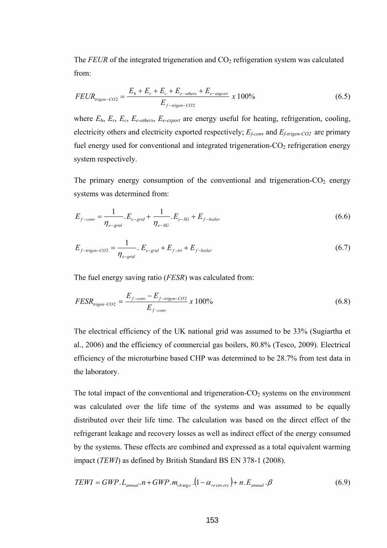
153

The FEUR of the integrated trigeneration and CO2 refrigeration system was calculated

from:

%1002

exp2 x

E

EEEEEFEUR

COtrigenf

orteothersecrhCOtrigen

(6.5)

where Eh, Er, Ec, Ee-others, Ee-export are energy useful for heating, refrigeration, cooling,

electricity others and electricity exported respectively; Ef-conv and Ef-trigen-CO2 are primary

fuel energy used for conventional and integrated trigeneration-CO2 refrigeration energy

system respectively.

The primary energy consumption of the conventional and trigeneration-CO2 energy

systems was determined from:

boilerfSGeSGe

gridegride

convf EEEE

.1

.1

(6.6)

boilerftrifgridegride

COtrigenf EEEE

.1

2 (6.7)

The fuel energy saving ratio (FESR) was calculated from:

%10022 x

E

EEFESR

convf

COtrigenfconvfCOtrigen

(6.8)

The electrical efficiency of the UK national grid was assumed to be 33% (Sugiartha et

al., 2006) and the efficiency of commercial gas boilers, 80.8% (Tesco, 2009). Electrical

efficiency of the microturbine based CHP was determined to be 28.7% from test data in

the laboratory.

The total impact of the conventional and trigeneration-CO2 systems on the environment

was calculated over the life time of the systems and was assumed to be equally

distributed over their life time. The calculation was based on the direct effect of the

refrigerant leakage and recovery losses as well as indirect effect of the energy consumed

by the systems. These effects are combined and expressed as a total equivalent warming

impact (TEWI) as defined by British Standard BS EN 378-1 (2008).

..1.... covarg annualeryreechannual EnmGWPnLGWPTEWI (6.9)

154

where:

GWP is the global warming potential of the refrigerant (kgCO2/kg); Lannual = the annual

refrigerant leakage (kg/year); mcharge = mass of the refrigerant charge (kg); = life time

refrigerant recovery factor; n = system operating time (years); Eannual = annual energy

consumption (kWh/year); and = CO2 emission factor (kgCO2/kWh).

To calculate the environmental impact of the supermarket some assumptions were

made. These are detailed in Table 6.1.

Table 6.1 Assumptions for TEWI calculation of the case study supermarket

Parameters AssumptionsReferences

Range SourceAnnual refrigerant leakage for centralised refrigeration system (% of charge)

15 15 - 30 TOC, 2006

Refrigerant charge for DX centralised refrigeration system: - Charged with HFC or HCFC (kg/kW refrigeration capacity)

3.5 2 - 5 MTP, 2008

- Charged with CO2 (kg/kW refrigeration capacity) 1.75 1 – 2.5 MTP, 2008 CO2 emissions factor: - Grid electricity (kgCO2/kWh) 0.547 DEFRA, 2009 - Natural gas (kgCO2/kWh) 0.184 DEFRA, 2009 Global warming Potential (100 years interval time horizon):

- R-404A (kgCO2/kg) 3900 TOC, 2006 - R-407C (kgCO2/kg) 1800 TOC, 2006 - R-744 (kgCO2/kg) 1 TOC, 2006 Refrigerant recovery factor (%) 70 Useful life of conventional and trigen-CO2 system (years)* 15

*Trigen-CO2 = integrated trigeneration and CO2 refrigeration system

66..33 EEnneerrggyy ppeerrffoorrmmaannccee ooff tthhee ccoonnvveennttiioonnaall ssyysstteemm

Simulation results of the conventional R-404A refrigeration system show an average

seasonal COP for the MT refrigeration of 2.51. The COP of the LT refrigeration system

was found to vary between 1.14 in the summer to 1.62 in winter, giving an average

seasonal value of 1.53. The combined seasonal COP of the LT and MT plant was

determined to be 2.17. A display of the conventional refrigeration model is given in

Figure L-1 (Appendix L).

Figure 6.8 shows the average daily fuel energy utilisation ratio (FEUR) of the

conventional supermarket energy system. It can be seen that the overall FEUR in winter

can reach 58% and then drops to about 44% in the summer due to lower heating

demand and higher electrical power consumption of the refrigeration systems, giving an

155

overall seasonal FEUR of 49.6%. The lower heating demand reduces the contribution of

the high efficiency gas boiler to the FEUR of the store. The higher electricity

consumption of the refrigeration systems counterbalances the reduction of the primary

fuel of the gas boiler which makes the primary fuel energy of the store relatively

constant all year round. The effect can also be seen from the FEURs for refrigeration

and electricity-others, which are quite stable throughout the year with annual averages

of 19% and 21.2% respectively.

Figure 6.8 Daily average fuel utilisation ratio of the conventional energy system

Annual average FEUR of space cooling is only 2.1% and heating 7.3% because of the

relatively low average demand for space cooling and heating respectively. The total

primary fuel energy required by the conventional system is 9,411 MWh per year,

90.7% arising from electricity use (Table 6.2).

66..44 EEnneerrggyy aanndd eennvviirroonnmmeennttaall ppeerrffoorrmmaannccee ooff tthhee ttrriiggeenneerraattiioonn--CCOO22

rreeffrriiggeerraattiioonn ssyysstteemm

The integrated trigeneration and CO2 refrigeration system employs 5 systems operating

in parallel each generating 80 kW of electrical power. This arrangement provides

optimum fuel utilisation ratio with average load factor 85% (calculated from useful heat

and total heat demand). The system can satisfy all refrigeration demand and 90% of the

heating demand. The remainder of the heat requirement is provided by an auxiliary gas

boiler system.

156

The daily variation of the FEUR of the system over a whole year is shown in Figure 6.9.

The annual average FEUR was found to be 55.7%, made up of 21.1% for refrigeration,

2.5% for space cooling, 7.9% for heating, 24.2% for electricity (electricity others =

21.5% and electricity export = 2.7%). The total fuel demand of the system was found to

be 8,081 MWh, providing savings of 1,331 MWh (14.14%) over the conventional

system (Table 6.2). The total electricity consumption of the store reduces by 17.7%

compared to the conventional system and most of the electricity consumption can be

satisfied by the local power generation system. Only 8% of the electricity is required to

be purchased from the national grid system. Because the control of the plant is based on

meeting the refrigeration demand, the system also generates excess electricity giving a

total electricity export to the grid of 261,221 kWh.

Figure 6.9 Daily average fuel energy utilisation ratio of the trigeneration-CO2 energy system

Table 6.2 summarises the energy performance of the conventional and trigeneration-

CO2 energy systems. It can be seen that the latter provides significant energy savings

over the conventional system. A detailed energy performance analysis of both energy

systems is given in Appendix M.

Table 6.3 shows a comparison between the CO2 emissions of the conventional and

trigeneration-CO2 systems for a 15% annual refrigerant leakage rate. It can be seen that

the trigeneration-CO2 energy system will result in annual emissions savings of 659 tCO2

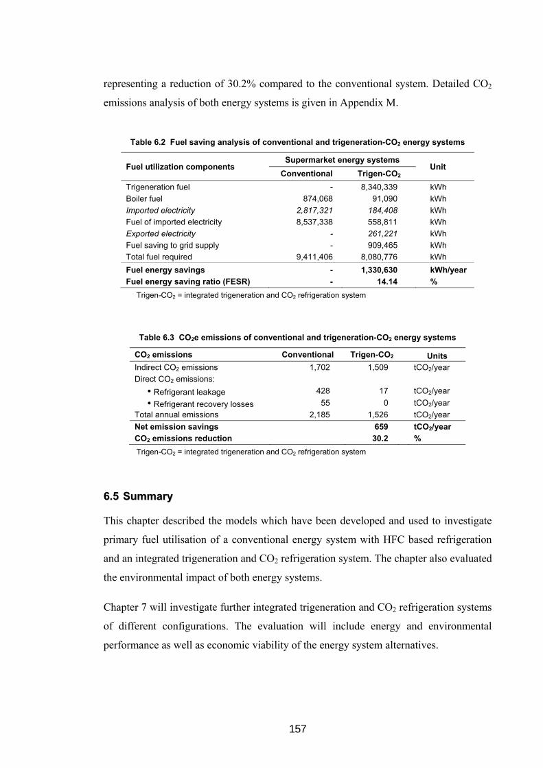
157

representing a reduction of 30.2% compared to the conventional system. Detailed CO2

emissions analysis of both energy systems is given in Appendix M.

Table 6.2 Fuel saving analysis of conventional and trigeneration-CO2 energy systems

Fuel utilization components Supermarket energy systems

Unit Conventional Trigen-CO2

Trigeneration fuel - 8,340,339 kWh

Boiler fuel 874,068 91,090 kWh

Imported electricity 2,817,321 184,408 kWh

Fuel of imported electricity 8,537,338 558,811 kWh

Exported electricity - 261,221 kWh

Fuel saving to grid supply - 909,465 kWh

Total fuel required 9,411,406 8,080,776 kWh

Fuel energy savings - 1,330,630 kWh/year

Fuel energy saving ratio (FESR) - 14.14 %

Trigen-CO2 = integrated trigeneration and CO2 refrigeration system

Table 6.3 CO2e emissions of conventional and trigeneration-CO2 energy systems

CO2 emissions Conventional Trigen-CO2 Units Indirect CO2 emissions 1,702 1,509 tCO2/year

Direct CO2 emissions:

• Refrigerant leakage 428 17 tCO2/year

• Refrigerant recovery losses 55 0 tCO2/year

Total annual emissions 2,185 1,526 tCO2/year

Net emission savings 659 tCO2/year

CO2 emissions reduction 30.2 %

Trigen-CO2 = integrated trigeneration and CO2 refrigeration system

66..55 SSuummmmaarryy

This chapter described the models which have been developed and used to investigate

primary fuel utilisation of a conventional energy system with HFC based refrigeration

and an integrated trigeneration and CO2 refrigeration system. The chapter also evaluated

the environmental impact of both energy systems.

Chapter 7 will investigate further integrated trigeneration and CO2 refrigeration systems

of different configurations. The evaluation will include energy and environmental

performance as well as economic viability of the energy system alternatives.

158

CChhaapptteerr 77

EENNEERRGGYY SSYYSSTTEEMM AALLTTEERRNNAATTIIVVEESS WWIITTHH IINNTTEEGGRRAATTEEDD TTRRIIGGEENNEERRAATTIIOONN AANNDD CCOO22 RREEFFRRIIGGEERRAATTIIOONN

This chapter investigates energy and environmental performance of integrated

trigeneration and CO2 refrigeration system alternatives for supermarket applications.

Different system arrangements are simulated and evaluated based on the energy demand

of the case study supermarket described in Chapter 6. The analysis compares the

performance of a conventional energy system using R-404A as the refrigerant, the

existing energy system in the store which utilises CO2 as refrigerant and alternative

trigeneration and CO2 refrigeration solutions.

77..11 SSuuppeerrmmaarrkkeett eenneerrggyy ssyysstteemm aalltteerrnnaattiivveess

Three schemes are considered which utilise different CO2 refrigeration and trigeneration

system arrangements. Scheme-1 is the system currently employed in the case study

supermarket and consists of: bio-fuel engine based CHP, sorption refrigeration system

and electric chiller for air conditioning, cascade transcritical CO2 refrigeration, and gas

boiler. Heat released by the CHP system drives the sorption chiller in a trigeneration

arrangement to generate cooling for the HVAC system. If cooling generated by the

trigeneration system is not enough to satisfy the space cooling needs, the balance is

provided by the electric vapour compression chiller with R-407C refrigerant. The

cascade transcritical CO2 refrigeration system is utilised to satisfy the MT and LT

refrigeration demands. The schematic diagram of the CO2 refrigeration system is as

159

shown in Figure 2.12 (Chapter 2). In this scheme, heat from the CO2 refrigeration

system is directly rejected to the atmosphere through an air cooled gas cooler. The heat

demand is satisfied by heat from the CHP system, when it is not used for cooling, and

the balance by the gas fired boiler. The electrical demand is satisfied by a combination

of local power generated by the CHP system and power imported from the grid. The

energy flow diagram of the energy system of Scheme-1 is shown in Figure 7.1.

Figure 7.1 Energy flow diagram of existing energy system (Scheme-1)

Scheme-2 is a supermarket energy system which integrates cascade transcritical CO2

refrigeration and trigeneration systems. The energy released by the gas engine CHP

system is used to drive a sorption chiller which is cascaded to a CO2 condenser to cool

and condense the CO2 refrigerant of the cascade transcritical CO2 refrigeration system.

Chilled water temperature from the sorption chiller of the trigeneration system is

considered to be at 7 oC. This integration arrangement is shown in Figure 7.2. It ensures

operation of the CO2 refrigeration system in the subcritical region but the system can

revert to transcritical operation in the event of trigeneration system failure.

Lighting, preparation, food, services, cabinets, others

MT refrigeration demand

LT refrigeration demand

Domestic hot water demand

Heating demand

Cooling demand HVAC

SUPERMARKET ENERGY

DEMAND

Bio-fuel Engine based CHP

Mix fuel

Bio-fuel

NG

CO2 Refrigeration

Pri

mar

y F

uel

ηe-grid

ηe-tri

ηth

Annual fuel

Ee-export

National grid

Ee-others

Ee-CO2

Ee-chiller

Ef-boiler

Absorption Chiller

Ee-tri

Ec R-407C Chiller

Ef-alternative

Eh

Ef-tri

Ee-grid

Er

Gas fired boiler

160

From Figure 7.2, it can be seen that the integration mode of Scheme-2 can be set by

opening valves SV1 and SV3; closing valve SV2; and switching off the ICMT valve.

This allows cooling from the trigeneration system to condense the CO2 gas in the HT

condenser. The liquid CO2 then flows from the condenser to the liquid receiver through

valve SV3 without expansion. When the ambient temperature is below 7 oC, valve SV1

can be closed and valve SV2 opened to allow the CO2 gas to be cooled by ambient air in

the air-cooled condenser. In order to switch the system to the transcritical operation

mode, valves SV1 and SV3 must be closed, valve SV2 opened; and the ICMT valve

energised.

Figure 7.2 Simplified schematic diagram of a cascade transcritical CO2 refrigeration integrated with trigeneration system (Scheme-2)

Scheme-3 is an improvement on the energy system considered in Chapter 6. It utilises

integrated CO2 refrigeration and trigeneration employing a high temperature sorption

chiller. A schematic diagram of scheme-3 is shown in Figure 7.3. The trigeneration

system consists of a natural gas engine based CHP system and a sorption refrigeration

system. The heat rejected by the CHP system is used to drive the sorption chiller, with

the cooling energy produced employed to condense the CO2 refrigerant of the

SV1 = solenoid valve of the HT condenser; SV2 = solenoid valve of the air cooled gas cooler/condenser; SV3 = bypass solenoid valve

MT display cabinets

LT pack

LT displaycabinets

HT pack

LT condenser

Air cooled gas cooler/ condenser

HT condenser

HTliquid

receiver

LT liquid receiver Cooling from

trigeneration

From other HT

packs

IHX

EXV

EXV

EXV

SV1

SV3

ICMT

ICM

SV2

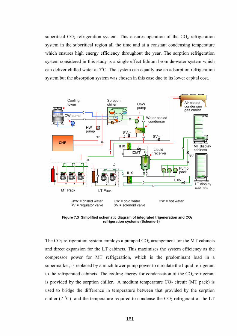
161

subcritical CO2 refrigeration system. This ensures operation of the CO2 refrigeration

system in the subcritical region all the time and at a constant condensing temperature

which ensures high energy efficiency throughout the year. The sorption refrigeration

system considered in this study is a single effect lithium bromide-water system which

can deliver chilled water at 7oC. The system can equally use an adsorption refrigeration

system but the absorption system was chosen in this case due to its lower capital cost.

Figure 7.3 Simplified schematic diagram of integrated trigeneration and CO2 refrigeration systems (Scheme-3)

The CO2 refrigeration system employs a pumped CO2 arrangement for the MT cabinets

and direct expansion for the LT cabinets. This maximises the system efficiency as the

compressor power for MT refrigeration, which is the predominant load in a

supermarket, is replaced by a much lower pump power to circulate the liquid refrigerant

to the refrigerated cabinets. The cooling energy for condensation of the CO2 refrigerant

is provided by the sorption chiller. A medium temperature CO2 circuit (MT pack) is

used to bridge the difference in temperature between that provided by the sorption

chiller (7 oC) and the temperature required to condense the CO2 refrigerant of the LT

ChW = chilled water CW = cold water HW = hot water RV = regulator valve SV = solenoid valve

MT display cabinets

LT Pack

HW pump

LT display cabinets

MT Pack

Liquid receiver

IHX

Water cooled condenser

IHX

Cooling tower

Sorption chiller

Pump pack

CW pump

ChW pump

Air cooled condenser/gas cooler

CHP

ICMT

SV

RV

EXV

SV

162

and MT circuits (-8 oC). To ensure operation of the refrigeration system in the event of

trigeneration system failure, the system design also employs a gas cooler which can be

brought into operation to take over from the sorption refrigeration system. The

arrangement can also provide an advantage of free cooling when the ambient

temperature is below 7 oC.

Figure 7.4 Energy flow diagram of energy system alternatives (Scheme-2 and Scheme-3)

Figure 7.4 shows the energy flow diagram of Schemes-2 and 3. In order to satisfy all

refrigeration demand of the store, the trigeneration system is modulated based on the

heat required by the sorption chiller to cool the CO2 refrigeration system. This also

means that the HVAC cooling demand is satisfied by an electric chiller with R-407C

refrigerant. A gas boiler is used to supply heat for the HVAC system and domestic hot

water system, if the heat from the trigeneration arrangement is not enough particularly

in the winter. The electrical demand is satisfied by a combination of local power

generated by the CHP system and power imported from the grid. In periods of excess

local power generation, the extra power is exported to the national grid.

CO2 refrigeration: Scheme-2 is a modified cascade transcritical CO2 refrigeration system; Scheme-3 is a modified volatile-DX CO2 refrigeration system

Lighting, preparation, food, services, cabinets, others

MT refrigeration demand

LT refrigeration demand

Domestic hot water demand

Heating demand

Cooling demand HVAC

SUPERMARKET ENERGY

DEMAND

Gas Engine based CHP

Mix fuel

NG

NG

CO2 Refrigeration

Pri

mar

y F

uel

ηe-grid

ηe-tri

ηth

Annual fuel

Ee-export

National grid

Ee-others

Ee-CO2

Ee-chiller

Ef-boiler

Absorption Chiller

Ee-tri

Ec R-407C Chiller

Ef-alternative

Eh

Ef-tri

Ee-grid

Er

Gas fired boiler

163

77..22 SSiimmuullaattiioonn mmooddeellss

Simulation models based on the Engineering Equation Solver (EES) software and a

spread sheet programme were established to determine the performance of the

alternative energy systems for the case study supermarket in terms of primary fuel

energy utilisation, GHG emissions and economic viability. Pressure - enthalpy diagrams

of the refrigeration systems applied in the schemes are shown in Figure 7.5. The

primary fuel energy utilisation ratio (FEUR) of the energy system alternatives can be

calculated from:

%100exp xE

EEEEEFEUR

ealternativf

orteothersecrhealternativ

(7.1)

The primary energy was determined from:

boilerftrifgridegride

ealternativf EEEE

.1

(7.2)

The fuel energy saving ratio (FESR) was calculated from:

%100xE

EEFESR

convf

ealternativfconvfealternativ

(7.3)

The payback period (years) is determined from:

savingnetAnnual

ealternativsystemenergyofinvestmentExtraPayback (7.4)

The electrical efficiency of the bio-fuel engine based CHP was assumed to be 35.1%

(Tesco, 2009) and the gas fuel engine based CHP to be 36.6% (Cogenco, 2008). Other

assumptions for the energy and environmental performance analysis are given in

Appendix N.

164

Figure 7.5 Thermodynamic models of the refrigeration system of Schemes 1 to 3 at ambient temperature of 27 oC

(c) Scheme-3: Modified volatile-DX CO2 refrigeration system cascaded with high temperature sorption chiller of a trigeneration system 4500

Enthalpy (kJ/kg)

-32oC

-8oC

Pre

ssu

re (

kPa

)

0.2 0.4 0.6 0.8

-500 -400 -300 -200 -100 0 100500

1000

10000

20000

43oCR-744

2800

1330

10oC

(a) Scheme-1: Cascade transcritical CO2 refrigeration system

-5oC

Enthalpy (kJ/kg)

-32oC

Pre

ssu

re (

kPa

)

0.2 0.4 0.6 0.8

-500 -400 -300 -200 -100 0 100500

1000

10000

20000

50oCR-744

2800

1330

80oC 32oC

-8oC

3200

8000

-3oC

(b) Scheme-2: Transcritical CO2 refrigeration system of Scheme-1 cascaded with high temperature sorption chiller of a trigeneration system

4500

Enthalpy (kJ/kg)

-32oC

-8oC

Pre

ssu

re (

kPa

)

0.2 0.4 0.6 0.8

-500 -400 -300 -200 -100 0 100500

1000

10000

20000R-744

2800

1330

10oC

50oC 43oC

-5oC3046

THE HIGH STAGE OF SCHEMES 2 AND 3 IS A TRIGENERATION SYSTEM WITH A HIGH TEMPERATURE SORPTION CHILLER FOR THE HEAT REJECTION

165

77..33 MMooddeell rreessuullttss aanndd ddiissccuussssiioonn

Scheme-1 is the current system in the supermarket which employs: i) a trigeneration

arrangement with bio-fuel engine based CHP of 200 kWe capacity; ii) a sorption chiller

with a cooling capacity 250 kWth; iii) 2 cascade transcritical CO2 refrigeration systems;

each system comprises of two HT circuits with MT load @ 38 kWth cascaded with an

LT circuit of capacity 25 kWth; iv) a 200 kWth R-407C electric chiller for air

conditioning and; v) 2 gas boilers of 200 kWth capacity each.

The COP of the cascade transcritical CO2 refrigeration system calculated using data

from the store was found to vary between 1.1 and 5.1 for MT system giving a seasonal

average COP of 2.4. The COP of the LT CO2 refrigeration system was in the range

between 2.5 and 4.9 with seasonal average COP of 3.5. The overall seasonal COP of the

cascade CO2 transcritical system was determined to be 2.5.

Figure 7.6 Daily average fuel energy utilisation ratio of scheme-1

Daily average fuel energy utilisation ratio (FEUR) of scheme-1 is shown in Figure 7.6.

It can be seen that the FEUR of refrigeration and electricity are quite stable throughout

the year with annual averages of 23% and 24% respectively, but the FEUR of heating

varies from 0% in the summer to 47% in winter giving a seasonal FEUR of 9.4%. The

figure also shows that the FEUR of cooling is relatively low with a seasonal average of

only 2.4%. Most of the cooling demand can be satisfied by the trigeneration

166

arrangement and only 1% is provided by the electric chiller. The arrangement has

average overall FEUR of 58.7%.

The energy analysis has also shown that with scheme-1, the trigeneration system can

satisfy 97.5% of the heat demand with only 2.5% provided by the gas boilers. The

electricity generated by the trigeneration arrangement in this scheme is 1,555 MWh

which is 57.3% of the total electricity requirement of the store. The annual primary fuel

requirement of scheme-1 is 7,967 MWh. Compared to the conventional energy system,

scheme-1 can provide primary fuel energy saving of 1,445 MWh with FESR of 15.3%

(Table 7.1).

Scheme-2 is a modification to the existing scheme of the case study supermarket. It

utilises a trigeneration arrangement with a 342 kWe gas engine based CHP and a

sorption chiller of 310 kWth integrated with a CO2 refrigeration plant similar to that of

Scheme-1. Scheme-2 also employs a 200 kWth R-407C refrigeration system for space

cooling and 2 x 200 kWth gas boilers for space and domestic hot water heating.

Figure 7.7 Daily average fuel energy utilisation ratio of scheme-2

Simulation results show a stable performance for both MT and LT refrigeration systems

all year round with COP of 5.4 and 4.1 respectively. This can provide an overall

seasonal COP of 5.0. With this arrangement, the CO2 refrigeration system can operate

subcritically at condensing temperature of 10 oC (assumed ΔT between chilled water

167

from the trigeneration and the liquid CO2 to be 3 K). A display of the EES simulation of

the CO2 refrigeration system is given in Figure L-2 (Appendix L).

Figure 7.7 shows the variation of the daily average FEUR of scheme-2. Overall FEUR

varies in the range 48.6% in the summer and 90% in winter with the average being

60.7%. Seasonal FEUR of electricity others, refrigeration, heating, cooling and export

electricity are 23.3%, 21.5%, 8.7%, 2.4% and 4.8% respectively. Total electricity

consumption of the store is 2,560 MWh which is 9.1% lower than the conventional

energy system. Scheme-2 will import 44 MWh and will export 378 MWh to the grid in

a year. The trigeneration arrangement generates electricity of 2,894 MWh. This scheme

was found to have a fuel energy saving ratio (FESR) of 24.7% compared to the

conventional system.

Preliminary sizing for an optimised trigeneration-CO2 refrigeration arrangement

(scheme-3) has shown the following system sizes to provide best results: trigeneration

arrangement with a 342 kWe gas engine based CHP and an absorption chiller with a

design cooling capacity of 310 kWth. Refrigeration capacity of 152 kWth for the MT

volatile CO2 refrigeration packs and 50 kWth refrigeration capacity for the LT packs.

The scheme is backed up by an electric 200 kWth capacity R-407C chiller for space

cooling and 2 x 200 kWth capacity gas boilers for heating.

Simulation on the modified volatile-DX CO2 refrigeration system integrated with the

trigeneration system also shows a stable performance for both MT and LT systems. The

COPs of the MT and LT systems are 5.0 and 5.6 respectively, giving an annual overall

COP of 5.1. Detailed simulation is given in Figure L-3 (Appendix L).

The daily variation of the FEUR of Scheme-3 over a whole year is shown in Figure 7.8.

The annual average FEUR of the scheme was found to be 64.4% comprising FEUR of

the electricity (for other services), refrigeration, heating and cooling of 25.1%, 23.1%,

9.2% and 2.6% respectively and FEUR of the export electricity of 4.4%. The scheme

has total fuel consumption 6,655 MWh, providing savings of 2,757 MWh (29.3%) over

the conventional system (Table 7.1). With Scheme-3, 96.8% of the electricity demand

of the supermarket can be satisfied by the local power generation system. The

trigeneration system can also satisfy 97% of the store’s heat demand with the remainder

supplied by the gas boiler system.

168

Figure 7.8 Daily average fuel energy utilisation ratio of scheme-3

Table 7.1 summarises the energy performance of the 3 alternative schemes. It can be

seen that all schemes provide significant energy savings over the conventional system

with scheme-3 resulting in the highest fuel savings and FESR.

Table 7.1 Results of fuel energy saving analysis

Fuel utilization components Supermarket energy systems

Unit Conventional Scheme-1 Scheme-2 Scheme-3

Trigeneration fuel - 4,431 7,907 7,450 MWh

Boiler fuel 874 21 194 25 MWh

Imported electricity 2,817 1,160 44 62 MWh

Fuel of imported electricity 8,537 3,515 135 189 MWh

Exported electricity - 0.12 379 333 MWh

Fuel saving to grid supply - 0.36 1,148 1,009 MWh

Total fuel required 9,411 7,967 7,088 6,655 MWh

Fuel energy savings - 1,444 2,323 2,756 MWh/year

Fuel energy saving ratio (FESR) - 15.3 24.7 29.3 %

(Detailed analysis is given in Appendix N)

Table 7.2 shows a comparison between CO2e emissions of the conventional and the

three energy system alternatives. The analysis assumed annual refrigerant leakage rate

of 15% of system charge. It can be seen that scheme-3 will lead to CO2e emissions

savings of 941 tCO2e which represents 43% savings over the conventional system.

169

Scheme-1 will result in savings of 1530 tCO2e mainly because of the use of bio-fuel and

the assumption that the emissions factor of bio-fuel is zero.

Table 7.2 CO2e emissions of investigated energy systems

CO2 emissions

Annual leakage 15% of charge Units

Conventional Scheme-1 Scheme-2 Scheme-3

Indirect CO2 emissions 1,702 638 1,308 1,227 tCO2/year

Direct CO2 emissions:

Refrigerant leakage 428 17 17 17 tCO2/year

Refrigerant recovery losses 55 - - - tCO2/year

Total annual emissions 2,185 655 1,325 1,244 tCO2/year

Net CO2 emissions saving 1,530 860 941 tCO2/year

70.0 39.4 43.1 %

(Detailed analysis is given in Appendix N)

77..44 EEccoonnoommiicc aannaallyyssiiss

To establish the economic viability of the energy system alternatives, prices of fuel

energy and the capital cost of the equipment were based on UK prices obtained from

equipment suppliers and end users. The results of the economic analysis are shown in

Table 7.3 for the installed cost and Table 7.4 for the annual energy and operational costs

of the conventional and alternative energy systems. Assumptions and data used in the

calculations are shown in Appendix O.

Table 7.3 Results of economic analysis: investment comparison

Cost components Supermarket energy system

Conventional Scheme-1 Scheme-2 Scheme-3

Installed cost (include VAT)

HT R-404A refrigeration packs £62,342.21

LT R-404A refrigeration packs £34,796.69

HT transcritical CO2 refrigeration packs £111,325.38 £111,325.38

MT Volatile-DX CO2 refrigeration packs £111,325.38

LT CO2 refrigeration packs £73,459.67 £73,459.67 £73,459.67

Electric chiller R-407C for air conditioning £29,375.00 £29,375.00 £29,375.00 £29,375.00

Gas boilers £47,000.00 £47,000.00 £47,000.00 £47,000.00

Gas engine based generator £67,812.19

Bio-fuel engine based CHP £158,625.00

Gas engine based CHP £271,248.75 £271,248.75

Water-LiBr absorption chiller £73,437.50 £91,091.68 £91,091.68

Total installed cost £241,326.08 £493,222.54 £623,471.29 £623,500.48

Extra investment £280,052.40 £382,145.21 £382,174.40

Calculation based on trigeneration capacity: Scheme-1 (current system): CHP = 200 kWe and sorption chiller = 250 kWth Schemes 2 and 3 (optimised capacity): CHP = 342 kWe and sorption chiller = 310 kWth (Assumptions used for investment cost analysis are shown in Table O-1, Appendix O)

170

Table 7.4 Results of economic analysis: annual energy and operational cost

Energy and operational cost components

Supermarket energy system

Conventional Scheme-1 Scheme-2 Scheme-3

Energy and operational cost (Incl. VAT)

Electricity cost/supplemental electricity cost £329,909.74 £135,828.75 £5,203.93 £7,300.44

Electricity sold back -£11.61 -£36,605.51 -£32,166.76

Fuel cost for operating boilers £28,431.62 £686.11 £6,321.38 £802.47

Bio-fuel cost for bio-fuel engine based CHP £216,163.36

Gas fuel cost for gas engine based CHP £257,181.29 £242,333.51

Standing charge £1,253.94 £1,253.94 £1,253.94 £1,253.94Availability charge (700 kVA of supply capacity)

£9,080.40 £9,080.40 £9,080.40 £9,080.40

Operation and maintenance cost £12,066.30 £32,592.38 £31,175.02 £31,175.02

Total energy and operational cost £380,742.01 £395,593.33 £273,610.99 £259,779.03

Annual net savings - £107,127.59 £120,962.98

Payback period (years) - 3.6 3.2

(Assumptions used for energy and operational cost analysis are given in Tables O-2 and O-3, Appendix O)

For the data used, it can be seen that scheme-3 will need additional investment of

£382,000 compared to the conventional energy system but will produce running cost

savings of the order of £121,000 per year, giving a payback period of 3.2 years.

Scheme-1 will require approximately the same annual energy and operational cost as the

conventional system due to the high cost of bio-fuel. The payback period of this scheme

will be very long. Scheme-2 provides annual running cost savings of the order of

£107,000. The payback period of Scheme-2 will be 3.6 years. The payback period is

strongly influenced by the ratio of electricity to gas prices known as the `spark ratio’.

Figure 7.9 Variation of payback period with spark ratio

3.2 years

Electricity price Spark ratio = Gas price

171

Figure 7.9 shows the variation of the payback period of scheme-3 with spark ratio. It

can be seen that the payback period drops sharply as the spark ratio increases with the

payback period reducing from 8 years at a spark ratio of 2.7 to 2.5 years at a spark ratio

of 4.0. The spark ratio in the UK varied between 2.7 and 4.6 in the period 2007-2009

(Moorjani, 2009). The spark ratio used in the analysis was 3.6 for natural gas and 2.4

for bio-fuel.

77..55 SSuummmmaarryy

This chapter has used modelling to investigate the energy and environmental

performance as well as economic viability of three supermarket energy system

alternatives. The energy system alternatives considered the application of trigeneration

and CO2 refrigeration systems of different arrangements including the integrated

trigeneration and CO2 refrigeration system proposed in this study. These investigations

have shown that the proposed energy system can provide substantial carbon savings and

a good payback period to HFC systems.

Chapter 8 will summarise the results and findings of the investigations in this study and

will provide some recommendations for future work.

172

CChhaapptteerr 88

CCOONNCCLLUUSSIIOONNSS AANNDD RREECCOOMMMMEENNDDAATTIIOONNSS FFOORR FFUUTTUURREE WWOORRKK

The environmental impact of the food retail industry, particularly supermarkets, is high

due to their high electrical energy consumption and indirect CO2 emissions from the

power stations and the direct emissions arising from refrigerant leakage to the

atmosphere. The use of CO2 as refrigerant offers the opportunity to reduce the direct

emissions.

The application of trigeneration can reduce the environmental impacts through a

substantial improvement in the overall energy efficiency over the conventional overall

supermarket energy approach. One solution through which the overall energy efficiency

of supermarkets can be increased and the environmental impacts reduced is through the

integration of trigeneration and CO2 refrigeration systems.

This thesis investigated experimentally and theoretically proof of concept of the

integration of trigeneration and CO2 refrigeration systems to maximise the reduction of

the environmental impacts of supermarkets. The concept combines the advantages of

CO2 refrigeration in reducing direct environmental impacts and trigeneration in

reducing indirect impacts through optimisation of fuel energy utilisation.

The research work involved the investigation and development of CO2 refrigeration

technologies for food retail refrigeration applications as well as the integration of CO2

refrigeration with trigeneration systems to eliminate the use of HFC refrigerants and

173

produce both energy savings and significant reductions in CO2 emissions. The work can

be detailed as follows:

Investigation of the advantages of CO2 as a refrigerant over HFC (hydro-

fluorocarbon) refrigerants including the investigation of design approaches for

CO2 refrigeration solutions for supermarket applications.

Analytical investigations to determine the refrigeration capacity for a test CO2

refrigeration system and its components and to evaluate the performance of the

CO2 refrigeration system and its integration with the trigeneration system.

Modelling and design of direct expansion and secondary CO2 coils for display

cabinet applications.

Design and construction of a primary low temperature and secondary medium

temperature CO2 refrigeration facility for frozen and chilled food refrigeration

applications including the integration of the facility with the trigeneration system.

Experimental investigation to establish the performance of the CO2 refrigeration

system and the performance of the integrated trigeneration and CO2 refrigeration

system.

Evaluation of the energy performance, environmental impacts and economic

viability of the integrated trigeneration and CO2 refrigeration systems in a case

study supermarket application.

This chapter summarises the findings arising from the research work and provides

recommendations for future work.

88..11 CCoonncclluussiioonnss

CO2 (R-744) is an environmentally benign refrigerant. It has an ODP of zero

and a very low global warming potential (GWP) of 1 which is much lower

than the GWP values of HCFC and HFC refrigerants. The CO2 refrigerant is non-toxic

and non-flammable which make it advantageous over other natural refrigerants such as

ammonia and hydrocarbons. Based on thermo-physical properties, theoretical

investigation of the comparative performance of CO2 and other refrigerants for

supermarket refrigeration applications showed that:

i) the CO2 refrigerant to provide good heat transfer in heat exchangers which

allows selection of smaller equipment than HCFC and HFC refrigerants;

11

174

ii) CO2 refrigeration systems to operate with low pressure ratio and operate with a

very small suction-gas specific volume and low pressure drop leading to

smaller size compressors and smaller suction pipe diameters for the same

operating conditions;

iii) the smaller components and pipe diameter that can be employed with CO2 lead

to a significant reduction in the refrigerant charge required for a given

refrigeration load compared to HCFC and HFC refrigerants;

iv) the main disadvantage of CO2 refrigerant to be its high working pressures.

This can be overcome by using smaller and stronger components.

CO2 refrigeration system solutions for supermarket applications fall into two

major categories: subcritical cascade systems and transcritical systems.

Subcritical cascade systems operate at moderate pressures and employ two refrigerants

one for refrigeration and another for heat rejection. Transcritical systems operate at high

pressures and high ambient temperatures but employ only CO2 as refrigerant. A

subcritical CO2 refrigeration system comprising a primary low temperature circuit for

frozen food refrigeration and a secondary medium temperature circuit for chilled food

refrigeration was identified to offer distinct advantages for an integrated trigeneration

and CO2 refrigeration system. With this arrangement, the trigeneration system is used to

condense the CO2 refrigerant vapour from both the LT and MT circuits and ensure

subcritical operation at all times.

Prior the construction of the CO2 refrigeration system and its integration with

the existing trigeneration system, an analytical investigation was performed to

determine the capacity of the CO2 refrigeration system and components. For this

purpose, mathematical models were developed for all components which influenced the

performance of the integrated system. The models were also used to investigate the

performance characteristics of the individual components and integrated system and

have led to the following results and conclusions:

1. The refrigeration capacity of the CO2 refrigeration system that matched with

the capacity of the existing trigeneration plant was determined to be 5 kW MT

refrigeration and 3 kW LT refrigeration.

22

33

175

2. The investigation of the performance of the CO2 refrigeration and integrated

systems at different condensing temperature showed that: i) increasing the

condensing temperature reduced the MT refrigeration capacity and increased

the pump power which subsequently reduced the COP of the MT refrigeration

system; ii) the increase of the condensing temperature also significantly

reduced the COP of the LT system and the overall COP of the refrigeration

system (combined LT and MT); iii) increasing the condensing temperature

enabled the absorption system to operate at higher delivery brine temperature

which improved the COP of the absorption and integrated systems.

3. The LT evaporating temperature was also found to affect the performance of

the CO2 refrigeration system. Increasing the LT evaporating temperature

improved the COP of the LT system but did not have any effect on the COP of

the MT system. The overall COP of the system increased slightly due to the

impact of the increase in the LT system COP. The load ratio of LT to MT

refrigeration in a system (LRLM) was also found to influence the overall COP

of the CO2 system. The overall COP increases with reducing LRLM.

4. The circulation ratio (CR) of the volatile MT system was found to influence the

COP of the MT and overall CO2 system. Increasing the circulation ratio above

the optimum of between 1.1 and 1.3 reduced the COP of the MT and the

overall CO2 system due to the power of the pump.

5. The COP of the integrated trigeneration-CO2 refrigeration system was found to

be highly depended on the COP of the sorption chiller.

Investigation of MT CO2 flooded evaporator coils and CO2 DX (direct-

expansion) evaporator coils for the MT and LT temperature levels was carried

out with simulation models developed using EES (Engineering Equation Solver)

software. The models were also used to design the geometry and tube arrangement of

evaporator coils for the test facility and were validated using data obtained from the

experimental investigations. The results showed:

i) for the same refrigeration duty the physical size of the flooded CO2 evaporator

coil was smaller compared to the direct expansion CO2 evaporator coil;

ii) increasing the evaporating temperature of the CO2 DX coil increased its

refrigeration capacity and reduced the pressure drop;

44

176

iii) increasing the circulation ratio of the flooded CO2 evaporator coil was found to

slightly improve the refrigeration duty of the coil but increased the refrigerant

mass velocity and pressure drop.

Investigation of the comparative performance of CO2 DX evaporator coils and

conventional coils using R-404A showed that for the same capacity and operating

conditions, the CO2 evaporator coils require smaller size and lower refrigerant charge

compared to coils using R-404A refrigerant.

Based on the simulation model results, the CO2 refrigeration system was

designed and integrated with the existing trigeneration system to form a

complete test facility. The test facility consists of three main modules: CHP module,

absorption refrigeration module and retail refrigeration system module. The CHP

module is based on an 80 kWe recuperated micro gas turbine generation package with

in-built boiler heat exchanger. The absorption refrigeration module is based on a

packaged direct gas fired ROBUR chiller which was re-engineered to operate with a

heat transfer fluid heated by the exhaust gases of the microturbine in the CHP module.

The retail refrigeration system module consists of a cascade volatile MT and direct

expansion LT CO2 refrigeration system and associated test facilities which include an

environmental test chamber and chilled and frozen food display cabinets located in the

chamber to provide controlled load to the refrigeration system. The test facility is

equipped with Danfoss controllers and was comprehensively instrumented for

monitoring and evaluation.

The test facility was used to investigate and evaluate the energy performance

of the CO2 refrigeration system as well as that of the overall trigeneration-CO2

refrigeration system. Tests were performed with different circulation ratios (CR) and

different evaporating temperatures for the MT CO2 refrigeration system. The

experimental test results demonstrated the following: i) the MT CO2 refrigeration

system was found to be able to achieve very high COPs ranging from 32 to 60, due to

the low power consumption of the CO2 pump; ii) the increase in the circulation ratio

caused an increase in the power consumption of the pump and influenced the COP of

the MT system which was found to be in good agreement with the simulation results.

The optimum circulation ratio was found to be in the range between 1.1 and 1.3; iii) the

55

66

177

LT CO2 refrigeration system was found to deliver a steady state COP of 4.0; iv) the

average overall COP of the CO2 refrigeration system, MT and LT was found to vary in

the range between 5.5 and 6.

A simulation study was carried out to investigate the seasonal energy and

environmental performance of a supermarket energy system using an

integrated trigeneration-CO2 refrigeration based on similar equipment and arrangement

as the one used for the laboratory tests and consisting of: i) CO2 refrigeration system

with a DX refrigeration circuit for LT and a pumped CO2 circuit for MT; ii) a

trigeneration system with a microturbine based CHP and ammonia-water absorption

refrigeration system. The performance of the energy system was compared with the for

a conventional energy system with R-404A parallel refrigerant circuits for MT and LT.

The integrated trigneration-CO2 refrigeration system was found to provide energy

savings of the order of 15 % and CO2 emission savings of the order of 30% compared to

the conventional energy system.

Further investigations were carried out to optimise the configuration of

trigeneration and CO2 refrigeration systems for supermarkets. Three

supermarket energy system alternatives to a conventional system were investigated

using experimental data from the test facilities and simulation studies. The results

indicated that:

1. Integration of CO2 refrigeration with trigeneration systems can produce

significant energy and GHG emission savings over conventional systems that

utilise electricity from the national grid and thermal energy from gas fired

boilers.

2. From the 3 alternative systems investigated, the most energy efficient

configuration was found to be the one that utilises a trigeneration system based

on a natural gas engine based CHP system and a single effect lithium bromide

water sorption system which can deliver chilled water at 7 oC. The cooling

produced by the sorption system of the trigeneration plant is used to condense

the CO2 refrigerant of the MT and LT refrigeration systems. The MT system is

a secondary ‘volatile’ pumped system whereas the LT system is a direct

expansion system. To bridge the difference in temperature provided by the

sorption system and that required to condense the CO2 refrigerant of the LT

77

88

178

and MT circuits, an MT CO2 compressor pack is used to operate between the

two temperature levels of 7 oC delivered by the sorption system and the -8 oC

condensing temperature required by the CO2 system. This system was shown to

provide fuel energy savings of the order of 30% and CO2 emission savings of

43% compared to the conventional system. The payback period of the system

was found to be of the order of 3.2 years.

3. The use of bio-fuels to drive the trigeneration plant can be attractive in terms of

the overall reduction in GHG emissions. However, the cost of bio-fuels can be

higher than that of conventional fuels which would have a negative impact on

the economic attractiveness of the system.

The research work carried out during the course of this project makes a

contribution to the overall effort to reduce the energy consumption and

environmental impact of the food retail industry, particularly supermarkets, in the UK.

The work also delivered specific contributions as follows:

1. The individual test results in the laboratory on the performance of cascade

volatile - DX CO2 refrigeration and trigeneration systems improve confidence

in the performance of the individual technologies and integrated systems.

2. The design approach proposed, where CO2 refrigeration can operate

independently of tri-generation when needed, should improve confidence in the

reliability of practical application of the concept in supermarkets.

3. The models developed and knowledge gained enable the design and sizing of

systems for given applications to ensure maximum performance and utilisation

efficiency.

4. Very high performance of CO2 when used as a secondary fluid in flooded

evaporator systems can lead to significant energy savings for high frozen food

loads. The optimum circulation ratio was determined to be in the range 1.1 to

1.3.

5. The unique test facility developed enables the in-depth investigation and

optimisation of component and system designs and controls. Significant

knowledge has been gained from the difficulties encountered in the

commissioning of the facility and matching of the capacities of the various

99

179

components which is much more critical in CO2 refrigeration systems

compared to conventional R-404A systems.

6. Technical knowledge gained and already disseminated or to be disseminated

with further publications includes better understanding of the behaviour of CO2

as a heat transfer fluid in flooded and direct expansion evaporator coils in

display cabinets, component operational characteristics and efficiencies as well

as oil management system requirements for the high pressure compressors.

These provide significant contributions to the development of more efficient

and reliable CO2 refrigeration technologies.

88..22 RReeccoommmmeennddaattiioonnss ffoorr ffuuttuurree wwoorrkk

The experimental investigations carried out as part of this project were mainly

concentrated on obtaining test results for the validation of the component and system

models developed. The unique test facilities developed enable the detailed investigation

and optimisation of the performance of individual components in the system,

optimisation of the matching of the capacities of these components as well as

optimisation of the controls.

The evaporator coil models developed enable the prediction of frost accumulation on

the coils during operation of the refrigeration system. The predictions of the rate of frost

accumulation, however, were found to be lower than the actual test results and the

differences which can be due to a variety of reasons such as measurement inaccuracies,

and inaccuracies in the frost accumulation algorithms used from the literature need to be

investigated further. It will be more appropriate to develop frost formation and

accumulation algorithms based on controlled tests in the laboratory for both flooded and

DX CO2 evaporator coils and use these to optimise the defrost cycle.

The Circulation Ratio was found to be a key parameter of the performance of a

secondary CO2 refrigeration system because of its influence on the heat transfer of the

coil and the pump power. An optimum circulation ratio enables the secondary

refrigeration system to achieve very high two phase heat transfer coefficients.

Continuous automatic adjustment of the circulation ratio for each display cabinet and

the MT refrigeration system as a whole could lead to higher overall system COP and

180

further work should be carried out to investigate efficient and economical ways to

continuously control the circulation ratio in commercial applications.

CO2 refrigeration and trigeneration technologies are in their early stages of development

and many years of research and development work are still required both at component

and system level for these technologies to reach the state of development of

conventional systems. The facilities at Brunel and the design and simulation tools

developed will play a key role in these developments over the next few years.

181

RREEFFEERREENNCCEESS

Aidoun, Z., and Ouzzane, M., 2009. A model application to study circuiting and operation in CO2 refrigeration coils. Appl. Therm. Eng. 29, 2544-2553.

Arteconi, A., Brandoni, C., Polonara, F., 2009. Distributed generation and trigeneration: Energy saving opportunities in Italian supermarket sector. Appl. Therm. Eng. 29, 1735-1743.

ASHRAE Standard 34, 2007. Designation and safety classification of refrigerants. ASHRAE, Inc., Atlanta. 53 pgs.

ASHRAE Standard 62.1, 2007. Ventilation for acceptable indoor air quality. ASHRAE, Inc., Atlanta, 49 pgs.

ASHRAE Standard 15, 2007. Safety standard for refrigeration system. ASHRAE, Inc., Atlanta, 36 pgs.

ASHRAE, 2010. ASHRAE handbook of refrigeration. ASHRAE, Inc., Atlanta, 749 pgs.

ATMOsphere, 2010. How to bring natural refrigerants faster to market: A summary report. International workshop on Natural Refrigerants, Brussels, Belgium, 42 pgs.

Bansal, P.K., and Jain, S., 2007. Cascade systems: past, present, and future. ASHRAE Transactions 113, 245-252.

Bassols, J., Kuckelkorn, B., Langreck, J., Schneider, R., Veelken, H., 2002. Trigenera-tion in the food industry. Appl. Therm. Eng. 22, 595–602.

Bayer, 2007. Diphyl-THT: High performance heat transfer fluid for pressureless operation. Available from http://www.bayer.com (accessed 03/06/2007).

Bell, K.J., and Mueller, A.C., 2001. Engineering data book II. Wolverine Tube, Inc., p. 230.

Bellstedt, M., 2008. Carbon dioxide systems for supermarkets review. Green Cooling Council (GCC), 5 pgs, available from: http://www.r744.com (accessed 23/07/2009).

Bellstedt, M., Elefsen, F., Jensen, S.S., 2002. Application of CO2 (R744) refrigerant in industrial cold storage plant. Forum, 25-30 (also available online from www.airah.org.au).

Bertelsen, P., and Christensen, K., 2003. Use of natural refrigerants in supermarkets. Danish Environmental Protection Agency.

Besant-Roberts, A., 2009. Tesco Thomas Street, Cheetham Hill, Great Manchester: Shortlisted for project of the year. Vinci Construction, UK.

Bingming, W., Huagen, W., Jianfeng, L., and Ziwen, X., 2009. Experimental investigation on the performance of NH3/CO2 cascade refrigeration system with twin-screw compressor. Int. J. Refrigeration 32, 1358-1365.

Bock, 2009. Product information HGX12P CO2 subcritical. Available from: http://www.bock.de.

Bodinus, W.S., 1999. The rise and fall of carbon dioxide systems. ASHRAE Journal, 37-42.

182

BS EN 12735-1, 2001. Copper and copper alloys, seamless, round copper tubes for air-conditioning and refrigeration: Part 1 - Tubes for piping systems. BSI, UK, 18 pgs.

BS EN 13136, 2001. Refrigerating systems and heat pumps: Pressure relief devices and their associated piping - methods for calculation, 28 pgs.

BS EN 378-1, 2008. Refrigerating systems and heat pumps - Safety and environmental requirements: Part 1 - Basic requirements, definitions, classification and selection criteria. BSI, UK, 68 pgs.

Campbell, A., Maidment, G.G., Missenden, J.F., 2006. A natural refrigeration system for supermarkets using CO2 as a refrigerant. Proc. CIBSE National Conference, London, UK.

Campbell, A., 2009. Working with CO2 supermarkets. Available from: http:// www.atmosphere2009.com/speakers.presentations.php (Accessed 14/01/2010).

Campbell, A., and Riley, O., 2009. Building services for low carbon supermarkets. Proc. Inst. R. 2009-10, 3/1-8.

CanmetENERGY, 2009. CO2 as a refrigerant in a Sobeys Supermarket, a case study. Natural Resources Canada, 8 pgs, available from: http://canmetenergy.nrcan.gc.ca (accessed 02/05/2010).

CCC, 2008. Building a low-carbon economy-The UK’s contribution to tackling climate change. The 1st report of the Committee on the Climate Change, 511 pgs, available from: http://www.theccc.org.uk (accessed 12/03/2010).

CCC, 2010. The fourth carbon budget, reducing emissions through the 2020s, 376 pgs, available from: http://www.theccc.org.uk (accessed 12/03/2010).

Chandrasekharan, R., Verma, P., Bullard, C.W., 2006. Development of a design tool for display case evaporators. Int. J. Refrigeration 29, 823-832.

Cheng, L., Ribatski, G., Moreno-Quiben, J., Thome, J.R., 2008a. New prediction methods for CO2 evaporation inside tubes: Part I - A two-phase flow pattern map and a flow pattern based phenomenological model for two-phase flow frictional pressure drops. Int. J. Heat and Mass Transfer 51, 111-124.

Cheng, L., Ribatski, G., Thome, J.R., 2008b. New prediction methods for CO2 evaporation inside tubes: Part II - An updated general flow boiling heat transfer model based on flow patterns. Int. J. Heat and Mass Transfer 51, 125-135.

CIBSE CHP Group, 2005. Spark ignition gas engine CHP. Available from: www.cibse.org/chp, (accessed 18/03/2009).

CIBSE Guide F, 2004. Energy efficiency in buildings. 2nd edition, London, The Chartered Institution of Building Services Engineers Publications, London, 261 pgs.

Cogenco, 2008. Cogenco cogeneration units 50 Hz range on natural gas. Available from: http://www.cogenco.com, (accessed 09/06/2010).

Coleman, H.W., and Steele, W.G., 2009. Experimentation, validation and uncertainty analysis for engineers. 3rd edition, John Wiley & Sons, Inc., ISBN: 978-0-470-16888-2.

183

Coulomb, D., 2008. Refrigeration and cold chain serving the global food industry and creating a better future: two key IIR challenges for improved health and environment. Trends in Food Science & Technology 29, 413-417.

Cowan, D., Chaer, I., Maidment, G., 2010. Reducing refrigerant emissions and leakage – An overview and feedback from two EU projects. Proc. Sustainable Refrigeration and Heat Pump Conference, Stockholm, Sweden, ISBN 978-2-913149-81-6, 16 pgs.

Danfoss, 2008a. Transcritical CO2 systems in a small supermarket. Available from www.danfoss.com/CO2 (accessed 12/01/2009).

Danfoss, 2008b. Product catalogue. Available from: www.danfoss.co.uk.

Danfoss, 2010. Experience significant savings with the Danfoss pumped CO2 solution. Available from www.danfoss.com/CO2 (accessed 28/11/2010).

Dean & Wood, 2011. Available from: http://dean-wood.com/products/refrigerant-price/ (accessed 22/04/2011).

DEFRA, 2005. The validity of food miles as an indicator of sustainable development: final report. ED50254, Issue 7, available from: http://statistics.defra.gov.uk/esg/ reports/foodmiles/default.asp/ (accessed 24/09/2009).

DEFRA, 2009. Guidelines to DEFRA / DECC’s GHG conversion factors for company reporting: Methodology paper for emission factors. DEFRA, London, 59 pgs.

Dopazo, J.A., Fernández-Seara, J., Sieres, J., and Uhía, F.J., 2009. Theoretical analysis of a CO2-NH3 cascade refrigeration system for cooling applications at low temperatures. Appl. Therm. Eng. 29, 1577–1583.

EES, 2010. Engineering equation solver. www.fChart.com

ESK Schultze, 2008. Components for CO2, available from: www.esk-schultze.de.

Estrada-Flores, S., 2010. Achieving temperature control and energy efficiency in the cold chain. Proc. 1st IIR International cold chain conference, Sustainability and the Cold Chain, Cambridge, workshop paper, ISBN 978-2-913149-75-5, 13 pgs.

Evans, J.A., 2008, Frozen food science and technology. FRPERC University of Bristol, UK, Blackwell Publishing Ltd, ISBN 978-1-4051-5478-9, 355 pgs.

Evans, J.A., 2010. Retail display. Proc. 1st Conference on Sustainability and the Cold Chain, Cambridge, UK, ISBN 978-2-9193149-75-5, workshop paper, 13 pgs

Fernandez-Seara, J., Sieres, J., and Va´zquez, M., 2006. Compression-absorption cascade refrigeration system. Appl. Therm. Eng. 26, 502-512.

Gartshore, J., and Benton, S., 2010. Cool concerns and Waitrose to support the use of hydrocarbons. Available from: http://www.hydrocarbons21.com/content/articles/ 2010-07-22-cool-concerns-and-waitrose-to-support-the-use-of-hydrocarbons.php.

Getu, H.M., and Bansal, P.K., 2007. Modeling and performance analyses of evaporators in frozen-food supermarket display cabinets at low temperatures. Int. J. Refrigeration 30, 1227-1243.

Getu, H.M., and Bansal, P.K., 2008. Thermodynamic analysis of an R744–R717 cascade refrigeration system. Int. J. Refrigeration 31, 45-54.

184

Girotto, S., Minetto, S., Neksa, P., 2004. Commercial refrigeration system using CO2 as the refrigerant. Int. J. Refrigeration 27, 717-723.

Heerup, C., 2009. Industrial systems. In: Reulens, W., Natural refrigerant CO2, KHLim, Belgium, 43-99.

Hinde, D., Shitong Zha, S., Lan, L., 2009. Carbon dioxide in North American supermarkets. ASHRAE Journal 51, 18-26.

Hinde, D., 2011. Applying natural refrigerants in supermarket refrigeration. ASHRAE winter conference, Las Vegas, USA, reported in: http://www.ammonia21.com.

Hong, K.T., and Webb, R.L., 1996. Calculation of fin efficiency for wet and dry fins. HVAC&R Research 2, 27-41.

IEA, 2009. World energy outlook. Available at http://www.worldenergyoutlook.org/ (accessed 03/12/2010).

IIR, 2000. 5th Informatory note on refrigerants: Carbon dioxide as a refrigerant. Available from www.iifiir.org (accessed 02/01/2009).

Inlow, S.W., and Groll, E.A., 1996. Analysis of secondary loop refrigeration systems using carbon dioxide as volatile secondary refrigerant. HVAC&R Research 2, 107-120.

IPCC, 2005. Safeguarding the ozone layer and the global climate system. UN-Intergovernmental Panel on Climate Change, 478 pgs, available from: http:// arch.rivm.nl/env/int/ipcc/pages_media/SROC-final/SpecialReportSROC.html (accessed 12/08/2008).

Ismail, K.A.R., and Salinas, C.S., 1999. Modelling of frost formation over parallel cold plates. Int. J. Refrigeration 22, 425-441.

ISO 23953-1, 2005. International Standard - Refrigerated display cabinets: Part 1 - Vocabulary, 36 pgs.

ISO 23953-2, 2005. International Standard - Refrigerated display cabinets: Part 2 - Classification, requirements and test conditions, 86 pgs.

Jiang, H., Aute, V., Radermacher, R., 2006. Coil designer: a general-purpose simulation and design tool for air-to-refrigerant heat exchangers. Int. J. Refrigeration 29, 601-610.

Jokar, A., Hayes, N., Ayub, Z.H., 2010. Recent developments in CO2 cascade condenser. Proc. Sustainable Refrigeration and Heat Pump Technology Conference, Stockholm, Sweden, 2010, 8 pgs.

Kakac, S., and Liu, H., 2002. Heat exchanger selection, rating and thermal design. 2nd edition, United State of America: CRC Press LLC.

Kays, W. M., and London, A. L., 1998. Compact heat exchangers. 3rd edition, Krieger Publishing, Malabar, FL.

Kim, N.H., Youn, B., Webb, R.L., 1999. Heat transfer and friction correlations for plain fin-and-tube heat exchangers. Proc. 11th Int. Heat Transfer Conference, Kyongju, Korea, 209-213.

185

Lawrence, J.M.W., and Gibson, D., 2010. Energy use across supermarket refrigeration. Proc. 1st IIR International cold chain conference, Sustainability and the Cold Chain, Cambridge, ISBN 978-2-913149-75-5, paper no. 242, 12 pgs.

Lee, T.S., Liu, C.H., Chen, T.W., 2006. Thermodynamic analysis of optimal condensing temperature of cascade-condenser in CO2/NH3 cascade refrigeration systems. Int. J. Refrigeration 29, 1100-1108.

Liang, S.Y., Wong, T.N., Nathan, G.K., 2001. Numerical and experimental studies of refrigerant circuitry of evaporator coils. Int. J. Refrigeration 24, 823-833.

Lidl, 2011. Two hundred Lidl stores to feature R290 technology by 2012. Available from: http://www.hydrocarbons21.com//content/articles/2011-01-14-200-lidl-stores-to-feature-r290-technology-by-2012.php.

Lommers, C.A., 2003. Air conditioning and refrigeration industry refrigerant selection guide. 7th ed. Melbourne, AIRAH, 66 pgs.

Lorentzen, G., 1995. The use of natural refrigerant: a complete solution to the CFC/HCFC predicament. Int. J. Refrigeration 18, 190-197.

M. Conde Engineering, 2002. Properties of working fluids–brines. Zurich, Switzerland, 9 pgs.

Maidment, G.G. and Tozer, R.M., 2002. Combined cooling heat and power in supermarkets. Appl. Therm. Eng. 22, 653-665.

Maidment, G.G., Zhao, X., Riffat, S.B. and Prosser, G., 1999. Application of combined heat and power and absorption cooling in a supermarket. Applied Energy 63, 169-190.

Maidment, G.G., Zhao, X. and Riffat, S.B., 2001. Combined cooling and heating using a gas engine in a supermarket. Applied Energy 68, 321–335.

Maidment, G.G., and Prosser, G., 2000. The use of CHP and absorption cooling in cold storage. Appl. Therm. Eng. 20, 1059–1073.

Mattsson, S.E., 1997. On modelling of heat exchangers in modelica. Proc. the 9th European Simulation Symposium, ESS'97, Oct 19-23, 1997, Passau, Germany.

Melinder, A., and Granryd, E., 2010. What to consider when using secondary fluids in indirect systems. Proc. Sustainable Refrigeration and Heat Pump Conference, Stockholm, Sweden, ISBN 978-2-913149-81-6, 12 pgs.

Met Office, 2009. Weather data for the London and Manchester area of the United Kingdom. Available from: www.metoffice.gov.uk

Moorjani, M., 2009. CHP in industrial and commercial sectors, a case study. Available from: http://chp.decc.gov.uk/cms/presentations-archive/ (accessed 03/09/2010).

Moreno-Quiben, J., and Thome, J.R., 2007a. Flow pattern based two-phase frictional pressure drop model for horizontal tubes: Part I - Diabatic and adiabatic experimental study. Int. J. Heat and Fluid Flow 28, 1049-1059.

Moreno-Quiben, J., and Thome, J.R., 2007b. Flow pattern based two-phase frictional pressure drop model for horizontal tubes: Part II - New phenomenological model. Int. J. Heat and Fluid Flow 28, 1060-1072.

186

MTP, 2008. BNCR36: Direct emission of refrigerant gases. Market Transformation Programme, available from: http://efficient-products.defra.gov.uk/cms/product-strategies/subsector/commercial-refrigeration (accessed 24/12/2009).

Navarro, E., Granryd, E., Urchueguia, J.F., Corberan, J.M., 2007. A phenomenological model for analyzing reciprocating compressors. Int. J. Refrigeration 30, 1254-1265.

PAS 2050, 2008. Specification for the assessment of the life cycle greenhouse gas emissions of goods and services. BSI Group, London, 43 pgs, available from: http://shop.bsigroup.com/en/Browse-by-Sector/Energy-Utilities/PAS-2050/ (accessed 03/12/2010).

Pearson, A., 2005. Carbon dioxide - new uses for an old refrigerant. Int. J. Refrigeration 28, 1140-1148.

Pearson, A., 2008. Refrigeration with Ammonia. Int. J. Refrigeration 31, 545–551.

PolySMART, 2008. Polygeneration in Europe – a technical report. 200 pgs, available from: http://www.polygeneration.org/.

Proklima, 2008. Natural refrigerants. GTZ GmbH, Eschborn, Germany, 208 pgs.

Rhiemeier, J.M., Harnisch, J., Ters, C., Kauffeld, M., Leisewitz, A., 2009. Comparative assessment of the climate relevance of supermarket refrigeration systems and equipment. Federal Environment Agency, 270 pgs, available from: http:// www.umweltbundesamt.de.

Riffat, S.B., Afonso, C.F., Oliveira, A.C., Reay, D.A., 1997. Natural refrigerants for refrigeration and air-conditioning system. Appl. Therm. Eng. 17, 33-42.

Rivet, P., 2002. A green and up to date retail store. Proc. International Conference New Technologies in Commercial Refrigeration, Urbana, IL, USA, pp. 31-34.

Robur, 2006. Gas fired absorption chiller for cooling medium-large area: installation, use and maintenance manual. 7th edition, available from http://www.robur.com (accessed 30/05/2007).

Rogstam, J., 2010. Ice rinks using carbon dioxide as secondary refrigerant. Proc. Sustainable Refrigeration and Heat Pump Conference, Stockholm, Sweden, ISBN 978-2-913149-81-6, 9 pgs.

Romero-Mendez, R., Sen, M., Yang, K.T., McClain. R., 2000. Effect of fin spacing on convection in plate fin and tube heat exchanger. Int. J. Heat and Mass Transfer 43, 39-51.

Sawalha, S., Soleimani, K.A., Rogstam, J., 2006. Experimental and theoretical evaluation of NH3/CO2 cascade system for supermarket refrigeration in laboratory environment. Proc. 7th IIR Gustav Lorentzen Conference on Natural Working Fluids, Trondheim, Norway.

Sawalha, S., 2008. Theoretical evaluation of transcritical CO2 systems in supermarket refrigeration. Part I: Modelling, simulation and optimization of two system solutions. Int. J. Refrigeration 31, 516-524.

Schmidt, T.E., 1945. La production calorifique des surfaces munies d’ailettes. Bulletin de l’Institut International du Froid, Annexe G-5; cited in: Hong, K.T., and Webb, R.L., 1996. Calculation of fin efficiency for wet and dry fins. HVAC&R Research 2, 27-41.

187

Schmidt, T.E., 1949. Heat transfer calculation for extended surfaces. Refrigerating Engineering 57, 351-357; cited in: Perrotin, T., and Clodic, D., 2003. Fin efficiency calculation in enhanced fin and tube heat exchangers in dry conditions. Proc. International Congress of Refrigeration, Washington, D.C., US, paper no. ICR-0026, 8 pgs.

Shah, R.K., and Seculic, D.P., 2003. Fundamental of heat exchanger design. John Wiley & Sons Inc., New Jersey, 564-574.

Shilliday, J.A., and Tassou, S.A., 2010. Numerical analysis of a plate fin and tube evaporator using the natural refrigerant CO2. Proc. 1st IIR International cold chain conference, Sustainability and the Cold Chain, Cambridge, ISBN 978-2-913149-75-5, 8 pgs.

SRC, 2001. Refrigerant evaporator (DX) coil. Available from: http://www.srcoils.com/ File/PDF/Evap%20Coil%20Primer.pdf (Accessed 12/03/2010).

SRC, 2010. Standard plate fin coil specifications. Available from: http://www.srcoils. com /wp-content/blogs.dir/1/files/2010/05/Coil_Specs_Nomenclature.pdf (accessed 12/03/2010).

Stoecker, W.F., 1998. Industrial refrigeration handbook. McGraw-Hill, 782 pgs.

Suamir, IN. and Tassou, S.A., 2010. Trigeneration and its integration with CO2 refrigeration systems for supermarket applications. In: the SIRAC meeting, Brunel University, 23rd June 2010, 17 pgs, available from: http://www.sirac.org.uk/.

Suamir, IN., Tassou, S.A., Hadawey, A., Chaer, I., Marriott, D., 2009. Investigation of the performance characteristics of an ammonia-water absorption chiller in a trigeneration system arrangement. Proc. HPC Conference, Berlin, Germany, ISBN 978-0-9563329-0-5, paper no. HPC430, 6 pgs.

Sugiartha, N., Tassou, S.A., Chaer, I., Marriott, D., 2008. Trigeneration in food retail: An energic, economic and environmental evaluation for a supermarket application. Appl. Therm. Eng. 29, 2624–2632.

Sugiartha, N., Chaer, I., Tassou, S.A., Marriott, D., 2006. Assessment of a micro-gas turbine based trigeneration system in a supermarket. Proc. The International Conference of Fluid and Thermal Energy Conversion, Jakarta, Indonesia, ISSN 0854 9346, 12 pgs.

Swain, M., 2006. Energy use in food refrigeration: calculation, assumptions and data sources. FRPERC JOB NO. 2006013, University of Bristol, 19 pgs.

Tassou, S.A., and Suamir, IN., 2010. Trigeneration – a way to improve food industry sustainability. Proc. SEEP 2010 Conference, Bari, ITALY, 14 pgs.

Tassou, S.A., Chaer, I., Sugiartha, N., Ge, Y.T., Marriott, D., 2007. Application of trigeneration systems to the food retail industry. Energy Conversion & Management 48, 2988-2995.

Tassou, S.A., Ge, Y., Hadawey, A., Marriott, D., 2011. Energy consumption and conservation in food retailing. Appl. Therm. Eng. 31, 147-156.

Tassou, S.A., Chaer, I., Sugiartha, N., Marriott, D., Suamir, IN., 2008. Trigeneration – a solution to efficient use of energy in the food industry. Proc. Inst. R. 2007-08 7/1-16.

188

Tassou, S.A., Lewis, J.S., Ge, Y.T., Hadawey, A., Chaer, I., 2010. A review of emerging technologies for food refrigeration applications. Appl. Therm. Eng. 30, 263-276.

Tesco, 2009. Available from: http://tesco_energyict.com/tesco_webclient/ (accessed 2010, username and password required).

Threlkeld, J.L., 1970. Thermal environmental engineering. 2nd edition, Prentice Hall Book Co., Englewood Cliffs, NJ, 1970, cited in: Getu, H.M., Bansal, P.K., 2007. Modelling and performance analyses of evaporators in frozen-food supermarket display cabinets at low temperatures. Int. J. Refrigeration 30, 1227-1243.

TOC, 2006. Report of the refrigeration, air conditioning and heat pumps. UNEP, Nairobi, 223 pgs.

Verdemar, 2010. The first supermarket in Latin America that uses CO2 as a refrigerant. 9 pgs, available from: http://www.r744.com (accessed 24/12/2010).

Walravens, F., Hailes, J., Cox, N., 2009. ChillingFacts: The big supermarket refrigeration scandal. EIA, London, 8 pgs, available from: www.chillingfacts.org.uk (accessed 20/11/2010).

Wang, C.C., Chang, Y.J., Hsieh, Y.C., Lin, Y.T., 1996. Sensible heat and friction characteristics of plate fin and tube heat exchanger having plane fins. Int. J. Refrigeration 19, 223-230.

Wojtan, L., Ursenbacher, T., Thome, J.R., 2005a. Investigation of flow boiling in horizontal tubes: Part I - A new diabatic two-phase flow pattern map. Int. J. Heat and Mass Transfer 48, 2955-2969.

Wojtan, L., Ursenbacher, T., Thome, J.R., 2005b. Investigation of flow boiling in horizontal tubes: Part II - Development of a new heat transfer model for stratified-wavy, dryout and mist flow regimes. Int. J. Heat and Mass Transfer 48, 2970-2985.

189

AAPPPPEENNDDIIXX AA::

TTrriiggeenneerraattiioonn ppllaanntt

This appendix presents the schematic diagram of the trigeneration plant prior integration

with CO2 refrigeration. The plant employs oil Diphyl-THT as heat transfer medium to

transfer the recovered heat from the CHP unit to the absorption chiller as described in

Chapter 1, Section 1.4.

Figure A-1 The trigeneration plant prior integration with CO2 refrigeration

Chilled fluid pump

Absorption Chiller

Microturbine power generator

HX

Display cabinet

Hot fluid pump

Exhaust gas

Dry blast cooling unit

T

T

V

V

TT

P

Generator jacket

RoburACF 60-00 LB

Modifiedgenerator

BowmanMTG80RC-G-R

Carter, multi-deck display cabinet with a brine/air HX as the evaporator coil

190

AAPPPPEENNDDIIXX BB::

MMaatthheemmaattiiccaall mmooddeell ooff iinntteeggrraatteedd ttrriiggeenneerraattiioonn aanndd CCOO22 rreeffrriiggeerraattiioonn

This appendix provides supporting equations used in the mathematical models. Key

equations of the model are presented in Chapter 3. The appendix also presents the

displays of the EES models of the integration arrangements, pipe sizing and the liquid

receiver.

HTF properties:

Best fit equations of the properties of oil Diphyl-THT (Bayer, 2007) used for heat

transfer fluid (HTF) of the trigeneration system:

1. Density (kg/m3) at temperature range 0 – 340 oC:

526696.1017.652245603.0 T (B.1)

Coefficient of correlation R2 = 1.0000

2. Specific heat transfer coefficient (kJ/kg.oC) at temperature range 0 – 340 oC:

465115098.1.003462118.0 TCp (B.2)

Coefficient of correlation R2 = 1.0000

3. Thermal conductivity (W/m.oC) at temperature range 0 – 340 oC:

109809175.0.10.5315.2 5 Tk (B.3)

Coefficient of correlation R2 = 0.9914

4. Dynamic viscosity (Pa.s) at temperature range 20 – 340 oC:

18701616277.1.0708312959.20 T (B.4)

Coefficient of correlation R2 = 0.9865

Temperature is in oC.

The equations of aqueous solution of the propylene glycol:

Density and specific heat of the propylene glycol can be determined from the equations

described in M. Conde Engineering (2002) as below:

215.273

2.47215.273

3.28015.273

8.9654.1824.508

brinebrinebrinebrine TTT

(B.5)

191

215.273

4787.015.273

939.115.273

715.06086.0476.4

brinebrinebrinebrine TTT

Cp (B.6)

Where:

ρbrine in kg/m3; Cpbrine in kJ/kg K; 2

oibrine

TTT

in K

ξ = mass fraction of propylene glycol in water (used ξ = 40%).

192

Fig

ure

B-1

A

dis

pla

y o

f th

e E

ES

mo

del

of

the

inte

gra

tio

n a

rran

gem

ent

for

com

po

nen

t si

zin

g

193

Fig

ure

B-2

E

ES

mo

del

of

pip

e si

zin

g a

nd

pre

ssu

re d

rop

sim

ula

tio

n

194

Figure B-3 Vertical liquid receiver model

195

AAPPPPEENNDDIIXX CC::

MMeecchhaanniiccaall ccoommppoonneennttss

This appendix provides drawing of the identification and numbering of the mechanical

control of the CO2 refrigeration system. The design drawings of the liquid receiver, MT

and LT evaporator coils are also presented.

Legend for the symbol used in the mechanical control drawing:

V = flow control valve

PS = pressure transducer

SV = Solenoid valve

AKV = Danfoss electronic expansion valve

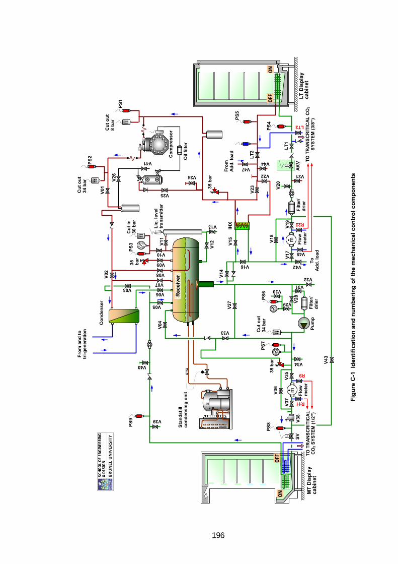
196

Fig

ure

C-1

Id

enti

fica

tio

n a

nd

nu

mb

erin

g o

f th

e m

ech

anic

al c

on

tro

l co

mp

on

ents

V45

LT

Dis

pla

y ca

bin

et

Fro

m a

nd

to

tr

i-g

ener

atio

n

m

TO

TR

AN

SC

RIT

ICA

L C

O2

SY

ST

EM

(3/

8”)

Co

nd

ense

r

IHX

AK

V

Liq

. le

vel

tran

smit

ter

Cu

t in

30

bar

P

S3

PS

6

35

bar

35 b

ar

Fil

ter/

dri

er

Flo

w

met

er

Sta

nd

still

co

nd

ensi

ng

un

it

MT

Dis

pla

y ca

bin

et

m

V38

Oil

filt

er

V20

V37

V

35

V36

V15

V02

V18

V17

V19

V23

V11

V10

Rec

eiv

er

V26

V06

V07

V08

V09

V05

V01

PS

9

PS

8 O

N

OFF

ON

O

FF

PS

5

PS

4

V12

V14

Cu

t o

ut

34 b

ar

PS

2

Cu

t o

ut

8 b

ar

PS

1

V27

V04

35 b

ar

Cu

t o

ut

34 b

ar

Pu

mp

V28

PS

7

LT

1

LT

2

V30

V29

V31

V32

V16

V13

V22

V44

V24

V25

Fil

ter/

dri

er

V33

Co

mp

ress

or

V34

V39

V40

V03

V41

V42

TO

TR

AN

SC

RIT

ICA

L

CO

2 S

YS

TE

M (

1/2”

)

V43

V21

To

Ad

d.

load

V47

Fro

m

Ad

d.

load

Flo

w

met

er

R22

R9

R11

LT2

SC

HO

OL

OF

ENG

INEE

RIN

G

& D

ESIG

N

BR

UN

EL U

NIV

ER

SIT

Y

SV

197

Fig

ure

C-2

L

iqu

id r

ecei

ver

wit

h t

he

mo

un

tin

g o

f th

e liq

uid

leve

l tra

ns

mit

ter

198

Technical data of the CO2 compressor:

(Source: Bock, 2009) CO2 pump specification: Manufacturer: HERMETIC-Pumpen GmbH Pump type Rotary vanes Model HTP 1-400 Rated flow 0.44 m3/h (approx. 108 gram/s at -8 oC) NPSH required 3.5 mLC Speed of pump 1450 rpm Test pressure 37.5 bar Suction port 3/8” (flange or weld connection) Discharge port 3/8” (flange or weld connection) Motor type 3 ph induction motor Power output 0.37 kW Voltage 230/400 Volt Frequency 50 Hz Motor speed 1450 rpm Frequency converter 1450-750 rpm approx. flow 0.44-0.22 m3/h Manufacturer details: Hermetic-Pumpen GmbH, Gewerbestrrasse 51 79194 Gundelfingen, Deutschland

Phone +49-761-5830-0; Fax: +49-761-5830-180 lederle@lederle-hermetic.com; http://www.lederle-hermetic.com

199

Fig

ure

C-3

P

late

hea

t ex

chan

ger

fo

r th

e C

O2 c

on

den

ser

200

Fig

ure

C-4

M

ediu

m t

emp

erat

ure

ev

apo

rato

r co

il

201

Fig

ure

C-5

L

ow

tem

per

atu

re e

vap

ora

tor

coil

202

AAPPPPEENNDDIIXX DD::

EElleeccttrriiccaall cciirrccuuiitt ddiiaaggrraammss ooff tthhee CCOO22 tteesstt ssyysstteemm

This appendix presents wiring diagrams of the electrical installation circuit and cabinet

controllers including electrical installation system of the additional load for the LT

refrigeration system. The wiring diagrams include:

Main electrical installation circuit

LT control circuit

MT control circuit

Standstill control circuit

Additional load control circuit

LT cabinet controller (EKC-414A1)

MT cabinet controller (EKC-204A1)

LT additional load evaporator controller (AK-CC-550)

203

Fig

ure

D-1

Wir

ing

dia

gra

m o

f th

e m

ain

ele

ctri

cal

inst

alla

tio

n c

ircu

it

204

Fig

ure

D-2

W

irin

g d

iag

ram

of

the

LT

co

ntr

ol

circ

uit

205

Fig

ure

D-3

W

irin

g d

iag

ram

of

the

MT

co

ntr

ol c

ircu

it

206

Fig

ure

D-4

W

irin

g d

iag

ram

of

the

stan

dst

ill c

on

tro

l ci

rcu

it

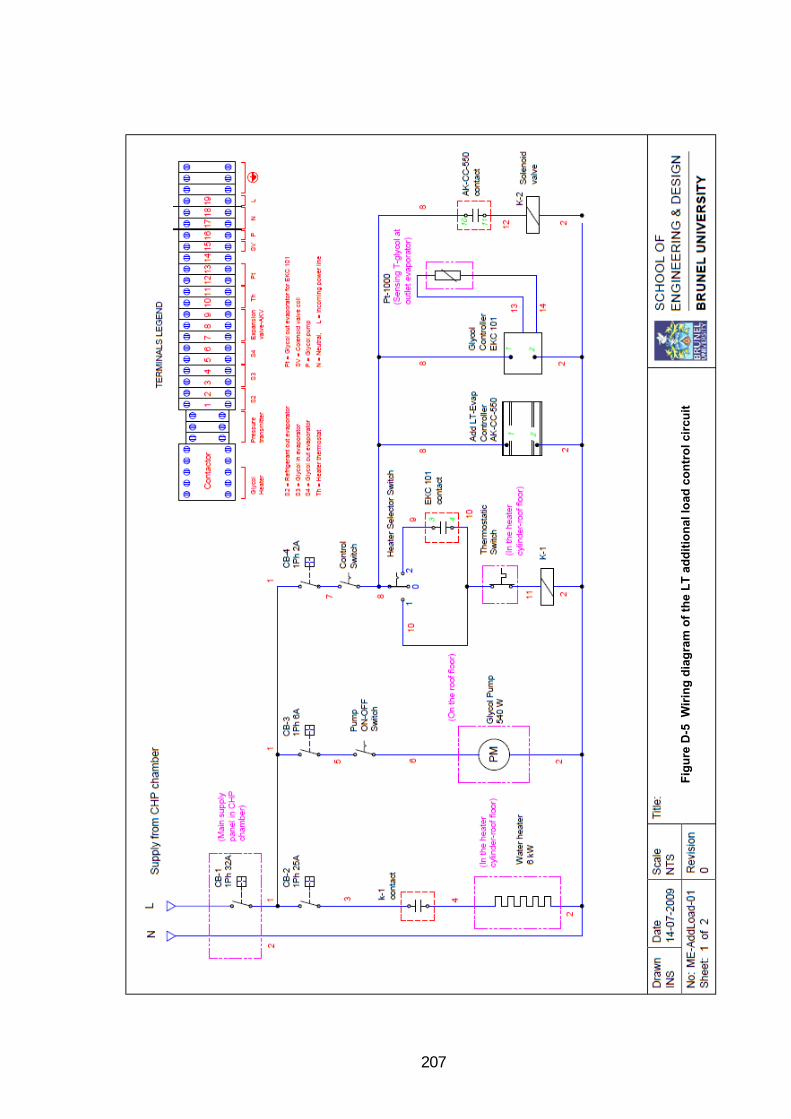
207

Fig

ure

D-5

W

irin

g d

iag

ram

of

the

LT

ad

dit

ion

al lo

ad c

on

tro

l ci

rcu

it

208

Fig

ure

D-6

E

KC

41

4A1

con

tro

ller

wir

ing

dia

gra

m

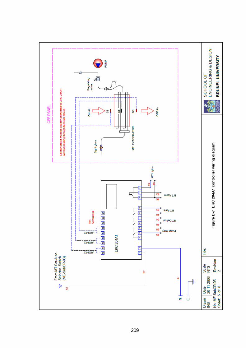
209

Fig

ure

D-7

E

KC

20

4A1

con

tro

ller

wir

ing

dia

gra

m

210

Fig

ure

D-8

A

K-C

C-5

50 c

on

tro

ller

wir

ing

dia

gra

m

211

AAPPPPEENNDDIIXX EE::

IInnssttrruummeennttaattiioonn aanndd ddaattaa llooggggiinngg ssyysstteemmss

This appendix provides the positions of the measurement points in the test rig, a display

of the monitoring system, identification of the measurement points and calibration

equations of the measurement devices.

Identification of the measurement points on the Datascan logger, which include the

measurement system of the subcritical and transcritical CO2 test rigs, is presented in

Table E-1.

Legend for Table E-1:

L = left

LT = low temperature

M = middle

MT = medium temperature

PS = pressure transducer for the subcritical test system

PT = pressure transducer for the transcritical test system

R = right

RH = relative humidity

SC = subcritical test system

T = temperature

TC = transcritical test system

The calibration equations of the thermocouples are presented in Table E-2 and the

graphs together with the calibration equations of the pressure transducers are shown in

Figure E-3.

212

Fig

ure

E-1

In

stru

men

tati

on

of

the

con

tro

l an

d m

on

ito

rin

g s

yste

ms

V45

LT

Dis

pla

y c

ab

ine

t

Re

ctif

ier

RH

X

Evaporator

Absorber Condenser

SCA-GAX

Desorber Oil

jac

ket

So

l. p

um

p

Ab

sorp

tio

n c

hill

er

Gly

col

pu

mp

V

m

TO

TR

AN

SC

RIT

ICA

L C

O2

SY

ST

EM

(3/

8”)

T

Co

nd

ense

r

IHX

EX

V

Liq

. le

vel

tran

smit

ter

Cu

t in

30

bar

P

S3

PS

6

35

bar

35 b

ar

Fil

ter/

dri

erF

low

m

eter

Flo

w

met

er

To

CH

P U

nit

Sta

nd

still

co

nd

ensi

ng

un

it

MT

Dis

pla

y ca

bin

et

m

V38

Oil

filt

er

V20

V37

V

35

V36

V15

V02

V18

V17

V

19

V23

V11

V10

Re

cei

ver

V26

V06

V07

V08

V09

V05

V01

Leg

end

:

SCH

OO

L O

F EN

GIN

EER

ING

&

DES

IGN

BR

UN

EL U

NIV

ER

SIT

Y

TT

T

T

T

T

T

T

T

T

T

T

T

T

T

PS

9

T

PS

8

T

T

T

T

T

ON

O

FF

ON

O

FF

PS

5

PS

4

V12

V14

T

T

Cu

t o

ut

34 b

ar

PS

2 C

ut

ou

t 8

bar

PS

1

V27

V04

35 b

ar

Cu

t o

ut

34 b

ar

Pu

mp

V28

PS

7

LT

1

LT

2

V30

V29

V31

V32

V16

V13

V22

V44

V24

V25

Fil

ter/

dri

er

V33

Co

mp

ress

or

V34

V39

V40

V03

= p

ress

ure

tra

nsm

itte

rs f

or

con

tro

l

= T

em

pe

ratu

re s

ens

ors

fo

r m

on

ito

rin

g a

nd

co

ntr

ol

V41

V42

TO

TR

AN

SC

RIT

ICA

L

CO

2 S

YS

TE

M (

1/2”

) V

43

V21

To

Ad

d.

load

V47

Fro

m

Ad

d.

load

Flo

w

met

er

R22

R9

R11

LT2

= p

res

sure

tra

nsm

itte

rs f

or

mo

nit

ori

ng

m V

= m

ass

flo

w-m

ete

r

= V

olu

me

flo

w-m

ete

r

SV

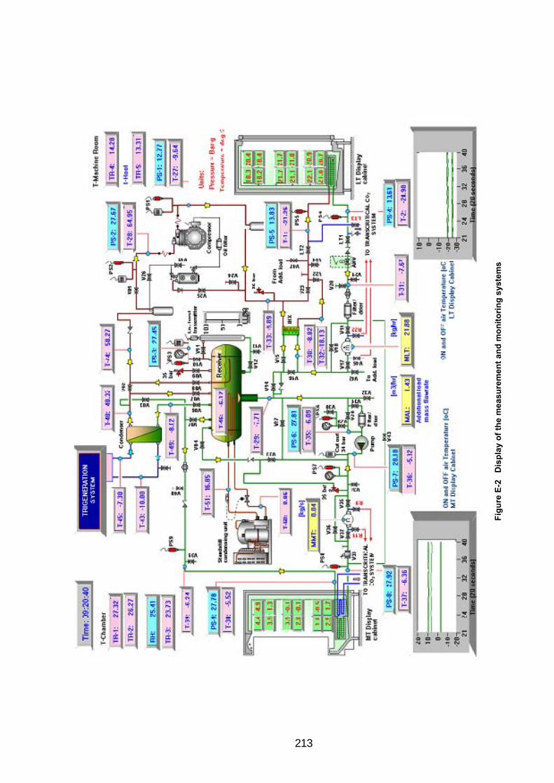
213

Fig

ure

E-2

D

isp

lay

of

the

mea

sure

men

t a

nd

mo

nit

ori

ng

sys

tem

s

214

Table E-1 Channel identification on the DataScan logger

Channel 

No.

Sensor 

No.

Description Channel 

No.

Sensor 

No.

Description

1 T27 SC Comp. IN 49 PT1 TC/SC Press. LT Evap. OUT

2 T28 SC Comp. OUT 50 PT2 TC Press. LT Comp. OUT

3 T29 Downleg pipe 51 PT3 TC Press. HT Comp.1a IN

4 T30 SC IHX‐hot OUT 52 PT4 TC Press. HT Comp.1b IN

5 T31 SC EXV IN 53 PT5 TC Press. HT Comp. OUT

6 T32 SC IHX‐cold IN 54 PT6 TC Press. GasCooler OUT

7 T33 SC IHX‐cold OUT 55 PT7 TC Press. ICMT IN

8 T34 SC Out regulator valve 56 PT8 TC Press. ICMT OUT

9 T35 SC Pump IN 57 PT9 TC Press. MT Evap. OUT

10 T36 SC Pump OUT 58 PT10 TC Press. MT Evap. IN

11 T37 SC MT Evap. IN 59 PT11 TC/SC Press. LT Evap. IN

12 T38 SC MT Evap. OUT‐1 60

13 T39 SC MT Evap. OUT‐2 61 MMT MT Flowmeter

14 T40 Ambient M. Room 62 LLV CO2 liquid level

15 T41 Brine evaporator chiller IN 63 MAL Add. Load Flowmeter

16 T42 Brine evaporator chiller OUT 64 MLT LT Flowmeter

17 T1 LT Evap. OUT 65 T43 Brine Condenser IN

18 T2 LT Evap. IN or EXV OUT 66 T44 SC Vessel IN from comp.

19 T2' LT EXV IN 67 T45 Brine Condenser OUT

20 T3 MT Air ON ‐ L 68 T46 SC Vessel‐Mid

21 T4 MT air OFF ‐ L 69 T47 SC Vessel‐Top

22 T5 TC Gas cooler IN 70 T48 SC Condenser IN

23 T6 TC Gas cooler OUT‐1 71 T49 SC Condenser OUT

24 T7 Ambient ‐ Roof 72 T50 Standstill TXV IN

25 T8 LT air ON ‐ L 73 T51 Standstill Evap. OUT

26 T9 LT air OFF ‐ L 74 T52 MT Air MID‐L

27 T10 TC LT‐Comp. IN 75 T53 MT Air ON‐M

28 T11 TC LT‐Comp. OUT 76 T54 MT Air ON‐R

29 T12 TC HT‐Comp.1a IN 77 T55 MT Air MID‐M

30 T13 TC HT‐Comp.1b IN 78 T56 MT Air MID‐R

31 T14 TC HT‐Comp. OUT 79 T57 MT Air OFF‐M

32 T15 TC ICMT IN 80 T58 MT Air OFF‐R

33 T16 TC Receiver OUT 81 T59 MT Bot‐Shelf‐Frnt‐L Up

34 T17 TC MT‐EXV IN 82 T60 MT Bot‐Shelf‐Frnt‐L Low

35 T18 TC MT‐EXV OUT or Evap IN 83 T61 MT Bot‐Shelf‐Rear‐L Up

36 T19 TC MT Evap. OUT‐1 84 T62 MT Bot‐Shelf‐Rear‐L Low

37 T136 T. Chamber‐1 85 T63 MT Bot‐Shelf‐Frnt‐M Up

38 T20 TC IHX2‐hot OUT 86 T64 MT Bot‐Shelf‐Frnt‐M Low

39 T21 TC MT Evap. OUT‐2 87 T65 MT Bot‐Shelf‐Rear‐M Up

40 T22 TC IHX3‐cold IN 88 T66 MT Bot‐Shelf‐Rear‐M Low

41 T23 TC Oil separator OUT 89 T67 MT Bot‐Shelf‐Frnt‐R Up

42 T24 TC GasCooler  OUT‐2 90 T68 MT Bot‐Shelf‐Frnt‐R Low

43 T25 TC Receiver‐Top or ICM IN 91 T69 MT Bot‐Shelf‐Rear‐R Up

44 T26 TC ICM OUT 92 T70 MT Bot‐Shelf‐Rear‐R Low

45 T137 TC ICMT OUT 93 T71 MT Mid‐Shelf‐Frnt‐L Up

46 T138 Add. Load IN 94 T72 MT Mid‐Shelf‐Frnt‐L Low

47 T139 Add. Load OUT 95 T73 MT Mid‐Shelf‐Rear‐L Up

48 T140 Brine add. Load IN 96 T74 MT Mid‐Shelf‐Rear‐L Low

Box 1: A

ll OFF

Box 2: S6 ON

Box 3: S5 ON

Box 4: S5 & S6 ON

Box 5: S4 ON

Box 6: S4 & S6 ON

215

Table E-1 Channel identification on the DataScan logger (Continued)

Channel 

No.

Sensor 

No.

Description Channel 

No.

Sensor 

No.

Description

97 PS‐1 SC Press. Compressor IN 145 T111 LT Mid‐Shelf‐Frnt‐L Up

98 PS‐2 SC Press. Compressor OUT 146 T112 LT Mid‐Shelf‐Frnt‐L Low

99 PS‐3 SC Press. Vessel 147 T113 LT Mid‐Shelf‐Rear‐L Up

100 PS‐6 SC Press. CO2 pump IN 148 T114 LT Mid‐Shelf‐Rear‐L Low

101 PS‐7 SC Press. CO2 pump OUT 149 T115 LT Mid‐Shelf‐Frnt‐M Up

102 PS‐8 SC Press. MT evap. IN 150 T116 LT Mid‐Shelf‐Frnt‐M Low

103 PS‐9 SC Press. MT evap. OUT 151 T117 LT Mid‐Shelf‐Rear‐M Up

104 152 T118 LT Mid‐Shelf‐Rear‐M Low

105 T75 MT Mid‐Shelf‐Frnt‐M Up 153 T119 LT Mid‐Shelf‐Frnt‐R Up

106 T76 MT Mid‐Shelf‐Frnt‐M Low 154 T120 LT Mid‐Shelf‐Frnt‐R Low

107 T77 MT Mid‐Shelf‐Rear‐M Up 155 T121 LT Mid‐Shelf‐Rear‐R Up

108 T78 MT Mid‐Shelf‐Rear‐M Low 156 T122 LT Mid‐Shelf‐Rear‐R Low

109 T79 MT Mid‐Shelf‐Frnt‐R Up 157 T123 LT Top‐Shelf‐Frnt‐L Up

110 T80 MT Mid‐Shelf‐Frnt‐R Low 158 T124 LT Top‐Shelf‐Frnt‐L Low

111 T81 MT Mid‐Shelf‐Rear‐R Up 159 T125 LT Top‐Shelf‐Rear‐L Up

112 T82 MT Mid‐Shelf‐Rear‐R Low 160 T126 LT Top‐Shelf‐Rear‐L Low

113 T83 MT Top‐Shelf‐Frnt‐L Up 161 T127 LT Top‐Shelf‐Frnt‐M Up

114 T84 MT Top‐Shelf‐Frnt‐L Low 162 T128 LT Top‐Shelf‐Frnt‐M Low

115 T85 MT Top‐Shelf‐Rear‐L Up 163 T129 LT Top‐Shelf‐Rear‐M Up

116 T86 MT Top‐Shelf‐Rear‐L Low 164 T130 LT Top‐Shelf‐Rear‐M Low

117 T141 Brine add. Load OUT 165 T131 LT Top‐Shelf‐Frnt‐R Up

118 T135 T. Chamber‐2 166 T132 LT Top‐Shelf‐Frnt‐R Low

119 RH‐LT OFF RH Air OFF LT 167 T133 LT Top‐Shelf‐Rear‐R Up

120 T‐LT OFF T Air OFF LT 168 T134 LT Top‐Shelf‐Rear‐R Low

121 T87 MT Top‐Shelf‐Frnt‐M Up 169 RH‐LT ON RH Air ON LT

122 T88 MT Top‐Shelf‐Frnt‐M Low 170 T‐LT ON T Air ON LT

123 T89 MT Top‐Shelf‐Rear‐M Up 171 RH‐1 RH Chamber pos. MT cab.

124 T90 MT Top‐Shelf‐Rear‐M Low 172 T‐142 T‐Chamber pos. MT cab.

125 T91 MT Top‐Shelf‐Frnt‐R Up 173 RH‐2 RH air OFF MT

126 T92 MT Top‐Shelf‐Frnt‐R Low 174 T‐143 T‐air OFF MT

127 T93 MT Top‐Shelf‐Rear‐R Up 175 RH‐3 RH air ON MT

128 T94 MT Top‐Shelf‐Rear‐R Low 176 T‐144 T‐air ON MT

129 T95 LT Air ON‐M 177

130 T96 LT Air ON‐R 178

131 T97 LT Air OFF‐M 179

132 T98 LT Air OFF‐R 180

133 T99 LT Bot‐Shelf‐Frnt‐L Up 181

134 T100 LT Bot‐Shelf‐Frnt‐L Low 182

135 T101 LT Bot‐Shelf‐Rear‐L Up 183

136 T102 LT Bot‐Shelf‐Rear‐L Low 184

137 T103 LT Bot‐Shelf‐Frnt‐M Up 185

138 T104 LT Bot‐Shelf‐Frnt‐M Low 186

139 T105 LT Bot‐Shelf‐Rear‐M Up 187

140 T106 LT Bot‐Shelf‐Rear‐M Low 188

141 T107 LT Bot‐Shelf‐Frnt‐R Up 189

142 T108 LT Bot‐Shelf‐Frnt‐R Low 190

143 T109 LT Bot‐Shelf‐Rear‐R Up 191

144 T110 LT Bot‐Shelf‐Rear‐R Low 192

Box 7: S4 & S5 ON

Box 8: S4, S5

 & S6 ON

Box 9: S3 ON

Box 10: S3 & S6 ON

Box 11: S3 & S5 ON

Box 12: S3, S5

 & S6 ON

216

Table E-2 Calibration equations of the thermocouples

General Equation:

Y = mX + bLegend:

Y = estimated actual value of temperature oC m = slope of Y and X corelation (linear regression)X = measured temperature by thermocouple b = constant or Y intercept

SE-m = Standard error of m R2 = coefficient of correlationSE-b = standard error of b SE-Y = standard error of estimated Y

Thermocouples m b R2 SE-m SE-b SE-Y

T27 0.996288 0.838253 0.998507 0.014559 0.241621 0.493266T28 0.996873 0.917977 0.998537 0.014424 0.238908 0.486442T29 0.997392 0.926840 0.998534 0.014443 0.239068 0.487008T30 0.996485 1.007307 0.998551 0.014348 0.237383 0.483115T31 0.996903 1.020488 0.998573 0.014244 0.235510 0.477880T32 0.998242 1.051715 0.998577 0.014242 0.235041 0.476889T33 1.000665 1.096362 0.998594 0.014190 0.233437 0.472780T34 1.001412 1.146833 0.998559 0.014377 0.236130 0.481116T35 0.996806 0.994470 0.998630 0.013952 0.230813 0.464066T36 0.995816 1.066011 0.998665 0.013760 0.227594 0.455604T37 0.998530 1.070330 0.998637 0.013943 0.229967 0.462488T38 0.998970 1.058034 0.998639 0.013941 0.229874 0.462081T39 0.998481 0.793385 0.998651 0.013870 0.229875 0.459045T40 0.998982 0.803464 0.998676 0.013749 0.227727 0.453003T41 1.011096 0.691332 0.998721 0.013674 0.224221 0.441661T42 1.011714 0.764923 0.998719 0.013693 0.224102 0.442168T5 1.003983 0.047941 0.998522 0.014597 0.244007 0.489775T6 1.005148 0.043130 0.998563 0.014411 0.240632 0.480171T7 1.005325 0.050396 0.998555 0.014455 0.241296 0.482145T20 1.006869 -0.227677 0.998509 0.014706 0.246498 0.492923T21 1.006422 -0.224810 0.998533 0.014578 0.244443 0.487189T22 1.006125 -0.244091 0.998509 0.014693 0.246538 0.492799T23 1.006597 -0.297907 0.998624 0.014124 0.237160 0.465705T24 1.006529 -0.313855 0.998572 0.014387 0.241658 0.478105T25 1.006209 -0.357100 0.998654 0.013964 0.234862 0.458439T26 1.007656 -0.377674 0.998653 0.013988 0.235025 0.458610

T137 1.005084 -0.366662 0.998594 0.014254 0.240039 0.472816T138 1.005240 -0.378429 0.998573 0.014363 0.241901 0.477865T139 1.005009 -0.385253 0.998653 0.013950 0.235045 0.458561T140 1.004826 -0.384303 0.998636 0.014034 0.236493 0.462631T141 1.002380 -0.259961 0.998428 0.015033 0.253269 0.511478T43 1.016260 -0.804837 0.998531 0.014733 0.247707 0.487759T44 1.009519 -0.678186 0.998561 0.014482 0.244441 0.480586T45 1.016917 -0.800334 0.998578 0.014503 0.243673 0.476630T46 1.008868 -0.656974 0.998564 0.014461 0.244128 0.480032T47 1.009174 -0.691975 0.998577 0.014400 0.243218 0.476978T48 1.009247 -0.663899 0.998545 0.014559 0.245720 0.484362T49 1.009185 -0.643462 0.998554 0.014515 0.244884 0.482338T50 1.008918 -0.643991 0.998617 0.014192 0.239512 0.467365T51 1.009197 -0.652264 0.998629 0.014132 0.238470 0.464343T52 1.009030 -0.610201 0.998620 0.014176 0.239044 0.466548T53 1.009542 -0.631277 0.998627 0.014149 0.238568 0.464918T54 1.008963 -0.642083 0.998610 0.014229 0.240122 0.469091T55 1.008861 -0.640687 0.998629 0.014129 0.238445 0.464440T56 1.008694 -0.644177 0.998636 0.014089 0.237835 0.462691T57 1.008963 -0.638842 0.998629 0.014128 0.238392 0.464319

217

Table E-2 Calibration equations of the thermocouples (Continued)

Thermocouples m b R2 SE-m SE-b SE-Y

T58 1.008353 -0.632173 0.998618 0.014180 0.239376 0.467158T59 1.010924 -0.713968 0.998634 0.014130 0.238358 0.463136T60 1.010447 -0.683936 0.998622 0.014188 0.239287 0.466155T61 1.010024 -0.676273 0.998612 0.014234 0.240130 0.468616T62 1.010466 -0.684766 0.998635 0.014122 0.238186 0.463080T63 1.010357 -0.663061 0.998589 0.014354 0.241993 0.473996T64 1.010359 -0.650000 0.998618 0.014204 0.239401 0.466969T65 1.010123 -0.649104 0.998658 0.013995 0.235931 0.457316T66 1.010484 -0.652083 0.998605 0.014277 0.240613 0.470312T67 1.009404 -0.710182 0.998674 0.013899 0.234807 0.453313T68 1.009879 -0.670779 0.998684 0.013857 0.233774 0.451000T69 1.010261 -0.669156 0.998646 0.014061 0.237126 0.460356T70 1.010034 -0.687574 0.998665 0.013955 0.235487 0.455528T71 1.007995 -0.665754 0.998666 0.013925 0.235336 0.455418T72 1.010419 -0.690479 0.998620 0.014197 0.239491 0.466630T73 1.008126 -0.638037 0.998600 0.014266 0.240923 0.471383T74 1.007786 -0.641638 0.998579 0.014370 0.242775 0.476490T75 1.005102 -0.607275 0.998627 0.014087 0.238461 0.464966T76 1.004906 -0.612683 0.998626 0.014087 0.238533 0.465089T77 1.004027 -0.614769 0.998643 0.013988 0.237078 0.461002T78 1.007630 -0.666963 0.998704 0.013719 0.231954 0.445984T79 1.004642 -0.728074 0.998748 0.013445 0.228298 0.434954T80 1.004826 -0.757554 0.998711 0.013645 0.231810 0.444304T81 1.006584 -0.752051 0.998690 0.013781 0.233677 0.449569T82 1.004779 -0.744378 0.998634 0.014044 0.238513 0.463123T83 1.006029 -0.584418 0.998579 0.014345 0.242465 0.476465T84 1.005678 -0.581317 0.998583 0.014319 0.242109 0.475517T85 1.005771 -0.596321 0.998569 0.014390 0.243355 0.478771T86 1.006373 -0.637317 0.998611 0.014187 0.239997 0.468812T87 1.008531 -0.728030 0.998594 0.014303 0.241921 0.472836T88 1.008854 -0.713885 0.998664 0.013946 0.235745 0.455869T89 1.007804 -0.727061 0.998614 0.014192 0.240217 0.468114T90 1.008799 -0.759998 0.998592 0.014320 0.242311 0.473447T91 1.007704 -0.766771 0.998573 0.014398 0.243926 0.477834T92 1.008302 -0.779651 0.998646 0.014031 0.237646 0.460198T93 1.008223 -0.777688 0.998601 0.014262 0.241564 0.471109T94 1.008354 -0.810320 0.998634 0.014096 0.238903 0.463240T95 1.008650 -0.554843 0.998736 0.013564 0.228542 0.438034T96 1.008062 -0.561418 0.998667 0.013918 0.234670 0.455046T97 1.008530 -0.568245 0.998700 0.013755 0.231847 0.447072T98 1.008026 -0.590051 0.998669 0.013907 0.234634 0.454541T99 1.008064 -0.597276 0.998625 0.014139 0.238586 0.465459

T100 1.007922 -0.627917 0.998693 0.013781 0.232735 0.448710T101 1.009413 -0.642028 0.998750 0.013499 0.227711 0.434516T102 1.008360 -0.648860 0.998661 0.013956 0.235698 0.456670T103 1.008867 -0.689146 0.998582 0.014370 0.242761 0.475750T104 1.008742 -0.708548 0.998650 0.014017 0.236935 0.459254T105 1.008667 -0.709277 0.998639 0.014076 0.237959 0.462092T106 1.008591 -0.734869 0.998597 0.014288 0.241689 0.472092T107 1.009206 -0.781258 0.998592 0.014325 0.242408 0.473401T108 1.009734 -0.805710 0.998640 0.014082 0.238312 0.461665T109 1.009126 -0.817441 0.998570 0.014431 0.244426 0.478462T110 1.008841 -0.837981 0.998583 0.014364 0.243462 0.475477T111 1.002716 1.175075 0.998613 0.014123 0.231555 0.468236T112 1.001583 1.203327 0.998668 0.013827 0.226858 0.454989T113 1.004092 1.157879 0.998680 0.013795 0.225936 0.451834

218

Table E-2 Calibration equations of the thermocouples (Continued)

Thermocouples m b R2 SE-m SE-b SE-Y

T114 1.000264 1.185578 0.998659 0.013853 0.227646 0.457071T115 1.003079 1.124538 0.998731 0.013516 0.221725 0.439331T116 1.000417 1.157030 0.998611 0.014103 0.231826 0.468816T117 1.003063 1.100321 0.998672 0.013825 0.226879 0.453925T118 1.003502 1.098576 0.998709 0.013638 0.223719 0.444799T119 1.005694 0.500755 0.998716 0.013632 0.225517 0.443111T120 1.005713 0.485195 0.998663 0.013908 0.230151 0.456134T121 1.005153 0.483058 0.998643 0.014006 0.231904 0.461107T122 1.002501 0.483082 0.998628 0.014044 0.233150 0.464658T123 1.005028 0.411832 0.998645 0.013995 0.232054 0.460646T124 1.002706 0.420698 0.998646 0.013953 0.231861 0.460208T125 1.003458 0.416978 0.998634 0.014027 0.232922 0.463183T126 1.002815 0.399485 0.998623 0.014077 0.233980 0.465973T127 1.001188 3.770771 0.998599 0.014174 0.225485 0.471645T128 1.000440 3.783498 0.998582 0.014250 0.226847 0.475766T129 1.001976 3.762256 0.998602 0.014171 0.225283 0.471002T130 1.002695 3.747141 0.998590 0.014242 0.226262 0.473842T131 1.002419 3.738011 0.998533 0.014522 0.230789 0.487273T132 1.002008 3.737103 0.998622 0.014069 0.223691 0.466133T133 1.002238 3.720344 0.998631 0.014025 0.222967 0.463892T134 1.002734 3.721418 0.998591 0.014235 0.226194 0.473507T135 1.001583 -0.195296 0.998405 0.015132 0.254790 0.516708

219

Table E-3 Pressure range of the pressure transducers and resistors used for data logging

General form of the best fit equations between the measured pressure and the output voltage of the pressure transducers is as follows:

y = mx + b

where y is the measured pressure (bar), x is the output voltage (V), b and m are a constant and rate of the pressure change with voltage respectively.

Figure E-3 Calibration graph and equation of the pressure transducers

NumberPS-1PS-2PS-3PS-4/PT-11PS-5/PT-1PS-6PS-7PS-8PS-9 500

Pressure range and resistor used

500250250500500500

0 to 18 bar 0 to 60 bar

Resistor (ohm)250500

0 to 30 bar 0 to 18 bar

Pressure range

0 to 30 bar

0 to 18 bar 0 to 60 bar 0 to 30 bar 0 to 30 bar

y = 4.486101x - 4.666069R² = 0.999991

0

5

10

15

20

25

0 1 2 3 4 5 6

Pre

ss

ure

(ba

r-g

)

Output Voltage (volt)

PS-1

y = 7.701956x - 15.708461R² = 0.999273

0

10

20

30

40

50

0 1 2 3 4 5 6 7 8

Pre

ss

ure

(ba

r-g

)

Output Voltage (volt)

PS-2

y = 7.612303x - 8.165438R² = 0.999323

0

10

20

30

40

50

0 1 2 3 4 5 6

Pre

ss

ure

(ba

r-g

)

Output Voltage (volt)

PS-3

y = 4.300600x - 4.229253R² = 0.999886

0

5

10

15

20

25

0 1 2 3 4 5 6 7

Pre

ss

ure

(ba

r-g

)

Output Voltage (volt)

PS-4/PT-11

220

Figure E-3 Calibration graph and equation of the pressure transducers (Continued)

y = 4.432440x - 4.549687R² = 0.999053

0

5

10

15

20

25

0 1 2 3 4 5 6

Pre

ss

ure

(ba

r-g

)

Output Voltage (volt)

PS-5/PT-1

y = 7.760145x - 16.889845R² = 0.999620

0

10

20

30

40

50

0 1 2 3 4 5 6 7 8 9

Pre

ss

ure

(ba

r-g

)

Output Voltage (volt)

PS-6

y = 9.426549x - 10.494319R² = 0.999450

0

10

20

30

40

50

0 1 2 3 4 5 6

Pre

ss

ure

(ba

r-g

)

Output Voltage (volt)

PS-7

y = 7.754203x - 9.284219R² = 0.999766

0

10

20

30

40

50

0 1 2 3 4 5 6

Pre

ss

ure

(ba

r-g

)

Output Voltage (volt)

PS-8

y = 7.810606x - 8.973765R² = 0.999320

0

10

20

30

40

50

0 1 2 3 4 5 6

Pre

ss

ure

(ba

r-g

)

Output Voltage (volt)

PS-9

221

AAPPPPEENNDDIIXX FF::

CCOO22 tteesstt cchhaammbbeerr

This appendix presents the layout of the CO2 test chamber including the position of the

LT and MT display cabinets. A display of the design of the air handling unit (AHU)

and a map of air velocity within the test area of the test chamber are also presented. The

following drawings are also included:

Layout of the CO2 test chamber with a 3.75 m long vertical door type cabinet

Layout of the CO2 test chamber with a 2.5 m long MT vertical open type cabinet

Layout of a possible extension of the test chamber

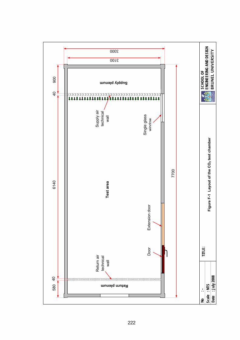
222

 

3300

3100

7700

Supply plenum

Return plenum 61

40

900

40

58

0

Tes

t ar

ea

40

ENG

INEE

RIN

G A

ND

DES

IGN

TI

TLE:

N

o : -

BR

UN

EL U

NIV

ER

SIT

Y

SCH

OO

L O

F

CO

2 tes

t cha

mbe

r lay

out

Scal

e : N

TS

Dat

e : J

uly

2008

Ret

urn

air

tech

nica

l w

all

Sup

ply

air

tech

nica

l w

all

Doo

r E

xten

sion

doo

r S

ingl

e g

lass

w

ind

ow

Fig

ure

F-1

Lay

ou

t o

f th

e C

O2 t

est

cham

ber

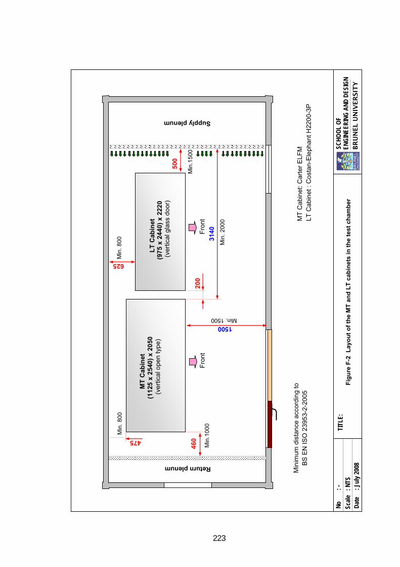
223

 

ENG

INEE

RIN

G A

ND

DES

IGN

TI

TLE:

N

o : -

BR

UN

EL U

NIV

ER

SIT

Y

SCH

OO

L O

F

MT

and

LT c

abin

et la

yout

in th

e te

st c

ham

ber

Scal

e : N

TS

Dat

e : J

uly

2008

Supply plenum

Min

. 80

0

1500 Min. 1500

LT

Cab

inet

(9

75 x

24

40)

x 22

20

(v

ertic

al g

lass

do

or)

460

Min

.10

00

475

500

Fro

nt

MT

Cab

inet

(1

125

x 2

540)

x 2

050

(v

ertic

al o

pen

typ

e)

Fro

nt

3140

Min

. 2

000

200

MT

Cab

inet

: Car

ter

ELF

M

Min

.15

00

Min

.80

0

625

Return plenum

Min

imum

dis

tanc

e ac

cord

ing

to

BS

EN

IS

O 2

395

3-2-

2005

LT

Cab

inet

: C

osta

n-E

leph

ant H

220

0-3P

Fig

ure

F-2

Lay

ou

t o

f th

e M

T a

nd

LT

cab

inet

s in

th

e te

st c

ham

ber

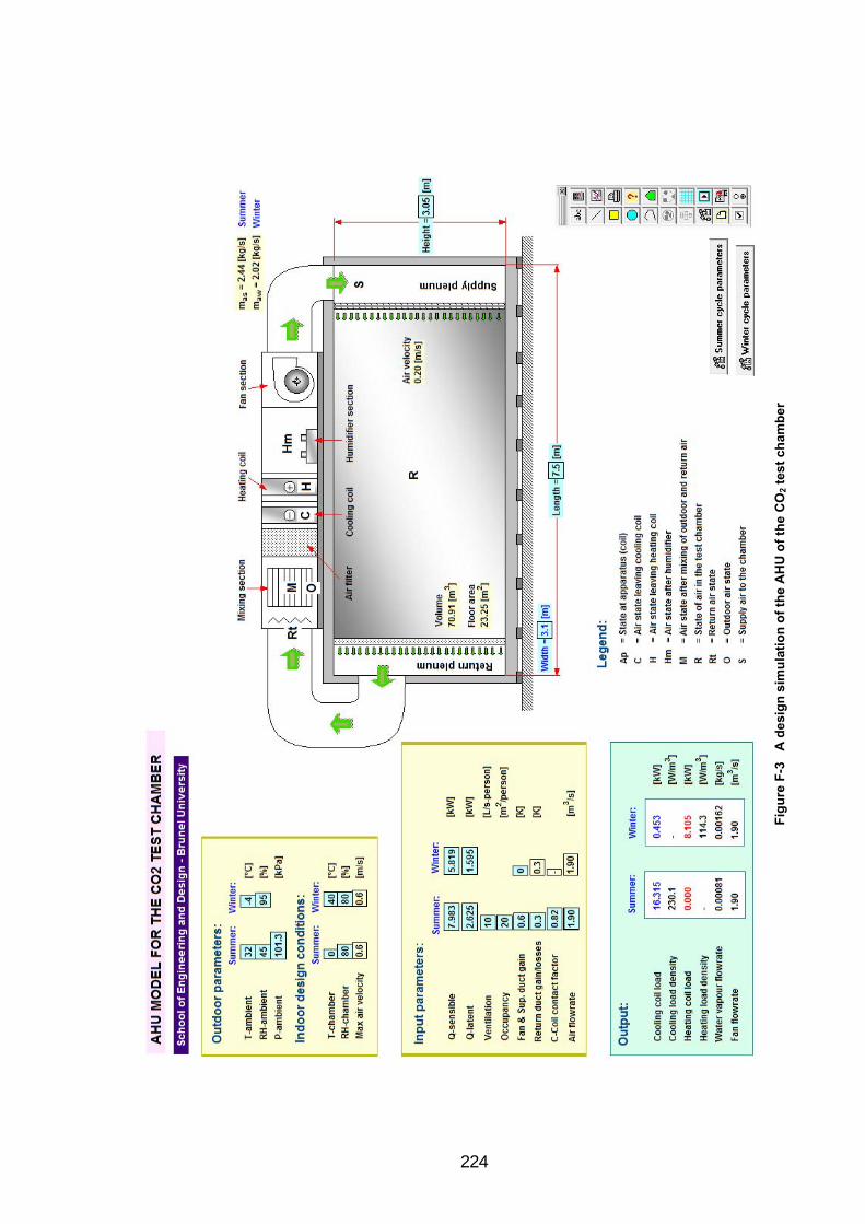
224

Fig

ure

F-3

A

des

ign

sim

ula

tio

n o

f th

e A

HU

of

the

CO

2 te

st c

ham

be

r

225

 

ENG

INEE

RIN

G A

ND

DES

IGN

Re

f. B

S E

N IS

O 2

395

3-2-

200

5

LT

Ca

bin

et

MT

Ca

bin

et

Return plenum

Supply plenum

CO

2 C

ha

mb

er

La

you

t A

A

B

B

600

Se

ctio

n A

– A

a b

c

de

1 2 3 4 5

Posi

tion

Air

velo

city

(m

/s)

a1

0.11

b1

0.

17

c1

0.12

d1

0.

14

e1

0.11

a2

0.

14

b2

0.18

c2

0.

15

d2

0.14

e2

0.

14

a3

0.18

b3

0.

20

c3

0.16

d3

0.

18

e3

0.18

a4

0.

17

b4

0.16

c4

0.

15

d4

0.18

e4

0.

17

a5

0.18

b5

0.

20

c5

0.20

d5

0.

18

e5

0.16

Se

ctio

n B

– B

Tes

ted

on t

he

18th

Ja

nua

ry 2

011

R

esu

lts

ba

sed

on

40

% f

an

sp

ee

d

f g

h

i

1 2 3 4 5

Posi

tion

Air

velo

city

(m

/s)

f10.

18g1

0.

18h1

0.

17

i10.

15f2

0.18

g2

0.19

h2

0.

18i2

0.15

f3

0.18

g3

0.

18h3

0.

19i3

0.

18

Posi

tion

Air

velo

city

(m

/s)

f4

0.13

g4

0.

20

h4

0.20

i4

0.

19

f5

0.10

g5

0.

14

h5

0.18

i5

0.

24

100

0

100

0

900

50

0

100

% c

om

ply

wit

h s

tan

da

rd

Me

asu

rem

en

t p

lan

e p

ara

llel t

o p

len

um

3D m

ea

sure

me

nt

86%

co

mp

ly w

ith

sta

nd

ard

TITL

E:

No

: -

(ro

tate

d t

o b

e f

loo

r a

t th

e b

ott

om

)

BR

UN

EL U

NIV

ER

SIT

Y

SC

HO

OL

OF

Mea

sure

d ai

r vel

ocity

in th

e CO

2 Cha

mbe

r S

cale

: N

TS

Dat

e : J

anua

ry 2

011

Fig

ure

F-4

Air

vel

oci

ty m

ap o

f th

e ai

r fl

ow

in t

he

CO

2 t

est

cham

ber

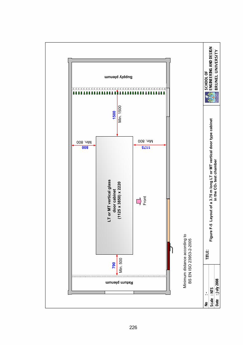
226

 

ENG

INEE

RIN

G A

ND

DES

IGN

TI

TLE:

N

o : -

BR

UN

EL U

NIV

ER

SIT

Y

SCH

OO

L O

F

CO

2 tes

t cha

mbe

r lay

out w

ith a

n LT

or M

T ve

rtic

al d

oor t

ype

cabi

net

Scal

e : N

TS

Dat

e : J

uly

2008

LT

or

MT

ver

tica

l gla

ss

do

or

cab

inet

(1

125

x 3

850)

x 2

220

Min

. 15

00

Min. 800 1175

Min. 800

790

Min

. 50

0

800

1500

Min

imum

dis

tanc

e ac

cord

ing

to

BS

EN

IS

O 2

395

3-2-

2005

Fro

nt

Supply plenum

Return plenum

Fig

ure

F-5

Lay

ou

t o

f a

3.75

m l

on

g L

T o

r M

T v

erti

cal

do

or

typ

e ca

bin

et

in t

he

CO

2 t

est

cham

ber

227

 

ENG

INEE

RIN

G A

ND

DES

IGN

TI

TLE:

N

o : -

BR

UN

EL U

NIV

ER

SIT

Y

SCH

OO

L O

F

CO

2 tes

t cha

mbe

r lay

out w

ith a

ver

tical

ope

n ty

pe M

T ca

bine

t Sc

ale

: NTS

D

ate

: Jul

y 20

08

Min

imum

dis

tanc

e ac

cord

ing

to

BS

EN

IS

O 2

395

3-2

-20

05

Min

. 20

00

Min. 800

1500

Min. 1500

1600

Min

. 1

00

0

MT

Cab

inet

(1

125

x 2

540

) x

20

50(v

ert

ica

l ope

n ty

pe)

475

2000

Fro

nt

Supply plenum

Return plenum

Fig

ure

F-6

Lay

ou

t o

f a

2.5

m l

on

g v

erti

cal

MT

op

en t

ype

cab

inet

in

th

e C

O2 t

est

cham

ber

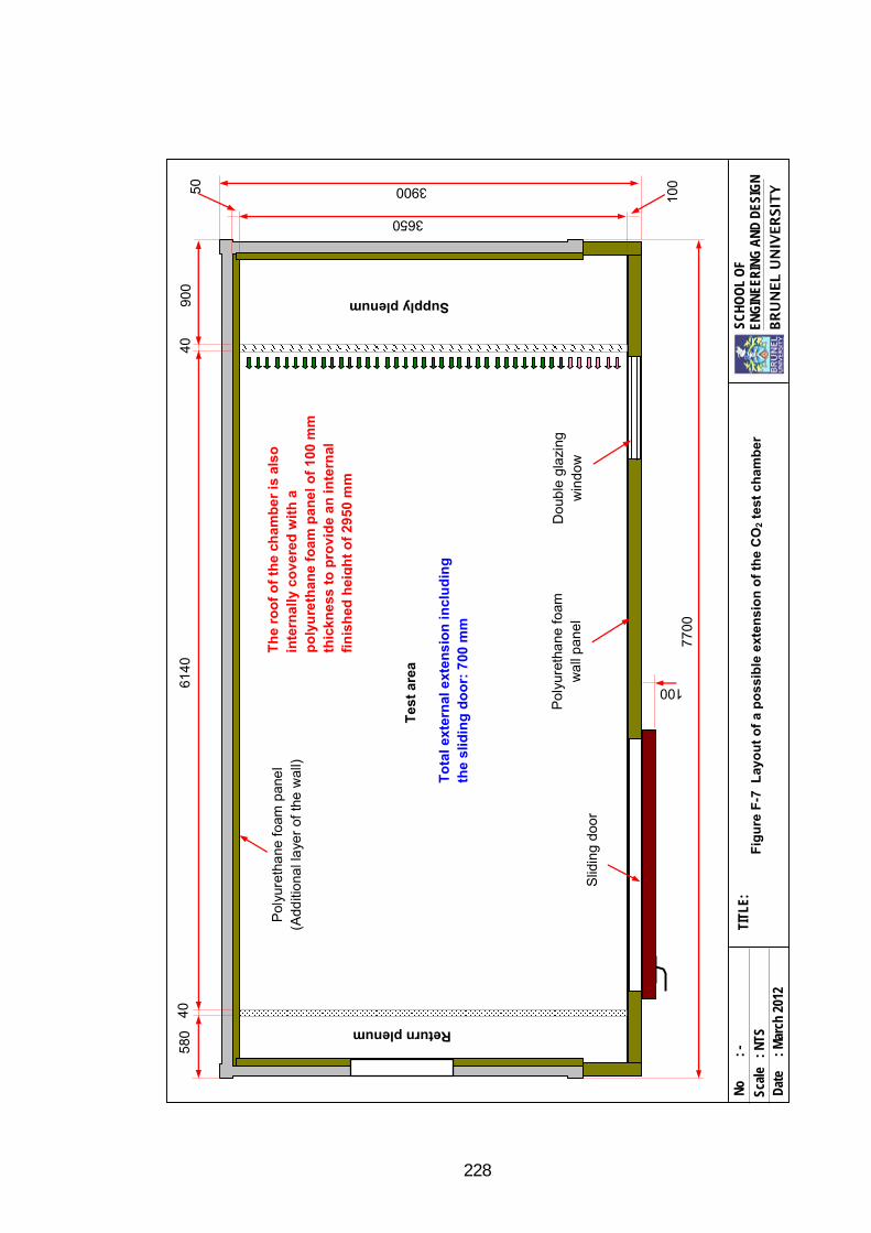
228

 

3900

3650

7700

Supply plenum

Return plenum 61

40

900

40

58

0

Tes

t ar

ea

40

50

100

100

Slid

ing

door

To

tal

exte

rnal

ext

ensi

on

in

clu

din

g

the

slid

ing

do

or:

700

mm

Dou

ble

gla

zing

w

ind

ow

P

olyu

reth

ane

foa

m

wal

l pa

nel

Pol

yure

tha

ne f

oam

pan

el

(Add

ition

al l

aye

r of

the

wal

l)

ENG

INEE

RIN

G A

ND

DES

IGN

TI

TLE:

N

o : -

BR

UN

EL U

NIV

ER

SIT

Y

SCH

OO

L O

F

CO

2 tes

t cha

mbe

r lay

out

Scal

e : N

TS

Dat

e : M

arch

201

2

Th

e ro

of

of

the

cham

ber

is

also

in

tern

ally

co

ver

ed w

ith

a

po

lyu

reth

ane

foa

m p

anel

of

100

mm

th

ickn

ess

to

pro

vid

e an

in

tern

al

fin

ish

edh

eig

ht

of

2950

mm

Fig

ure

F-7

Lay

ou

t o

f a

po

ssib

le e

xten

sio

n o

f th

e C

O2 t

est

cham

ber

229

AAPPPPEENNDDIIXX GG::

OOppeerraattiioonnaall mmooddeess aanndd pprroocceedduurreess

This appendix describes four modes of system operation. The valve arrangement for

each mode, operational procedures and some precautions are also presented.

The explanations in this appendix refer to Figure C-1 (Appendix C).

G.1 Operational modes

The operational arrangements refer only to the CO2 refrigeration system. The high stage

system is operating at steady state conditions at the designed delivery water glycol

temperature.

The four modes of the system operations can be described as below.

Normal operation mode:

The refrigerant circulates in both the LT and MT refrigeration systems. For the LT

circuit the refrigerant flows from the liquid receiver through the internal HX, LT flow

meter, LT evaporators (LT display cabinet and additional load), suction accumulator,

LT compressor, oil separator, condenser and returns back to the receiver as liquid.

For the MT circuit the liquid refrigerant circulates from the receiver to the CO2 pump

through the suction filter/drier. At discharge of the pump, the flow is divided into two

branches, one directly returns the liquid refrigerant back to the liquid receiver through

the bypass valve (V-33) and the other circulates the liquid through the MT flow meter,

regulator valve (V-38), MT evaporator and returns back to the receiver as a mixture of

liquid and vapour. The saturated vapour in the receiver circulates to the condenser

through a thermosiphon loop (valve V-07, condenser, and valve V-06). In this operation

the saturated vapour from the receiver is mixed with the hot gas from the LT circuit just

before entering the cascade condenser. The liquid from the condenser flows back into

the receiver by forced flow and gravity.

230

Valve arrangement for normal operation mode (Valve numbers refer to Figure C-1, Appendix C):

Valve no. V-01 V-02 V-03 V-04 V-05 V-06 V-07 V-08 V-09 V-10 V-11 V-12Position O O C O O O O C O O O O

Valve no. V-13 V-14 V-15 V-16 V-17 V-18 V-19 V-20 V-21 V-22 V-23 V-24Position C O O C O C O C C O C C

Valve no. V-25 V-26 V-27 V-28 V-29 V-30 V-31 V-32 V-33 V-34 V-35 V-36Position O O C C O C O C OR C O C

Valve no. V-37 V-38 V-39 V-40 V-41 V-42 V-43 V-44 V-45 V-47 Position O OR C C C O C C C O

C = closed; O = fully open; OR = open with manual regulation

Operation with thermosiphon condensation

In this operation, the hot gas from the discharge of the LT compressor passes through

the liquid receiver allowing the hot gas to be desuperheated by boiling some of the

liquid. The two-phase refrigerant from the MT circuit also terminates in the receiver.

The valve arrangement of the MT circuit is the same as in the normal operation mode.

The flow of the saturated vapour refrigerant from the receiver to the condenser occurs

solely due to the thermosiphon effect. The refrigerant vapour condenses in the

condenser and returns back to the receiver as a saturated liquid by gravity.

Valve arrangement:

Most of the valves are arranged as for normal operation mode except valve V-02 is

closed and valve V-08 is open.

Operation with forced condensation

The condensation of the CO2 refrigerant in the condenser occurs in forced flow

conditions. The condensation process is quite similar with the normal operation

arrangement but the flow rate of the refrigerant in this operation is higher. The hot gas

from the discharge of the LT compressor is connected in the same way as for normal

operation. The saturated liquid-vapour mixture from the MT circuit, however, is directly

circulated to the condenser after mixing with the hot gas from the LT circuit.

Valve arrangement:

The valves are arranged as those for normal operation except valve V-05 is closed and

valve V-03 is open.

231

Operation with gravity mode

The aim of the gravity mode is to investigate the performance of the MT system in

utilising the gravity force to circulate the liquid refrigerant and to provide refrigeration

effect to the MT display cabinet. In this operation, the MT evaporator is fed with liquid

refrigerant by gravity force. The pump is switched off. The bypass valve V-27 is open;

valves V-33 and V-31 are closed. The solenoid valve (SV) upstream of the MT

evaporator is in normal operation to enable the liquid refrigerant to flow through the

evaporator. The other valve arrangements remain the same for the normal operation

mode.

G.2 Operational procedures

The procedures consist of three stages which include starting up, testing and shutting

down. The test system is assumed to be fully charged; in standby conditions; the

standstill condensing unit is in operation to keep the CO2 refrigerant in the system; and

the test chamber is conditioned at 25 oC and 60% RH.

Starting up procedure

1. The procedure starts from the preparation of the high stage system (trigeneration

system or water chiller) and visual check of the whole integrated system.

2. Prepare the high stage system and check the setting point of the water-glycol

thermostat.

3. Position the control valves as set in the normal operation mode, except valves V-

14 and V-31 are closed.

4. Ensure the oil level of the LT compressor in the range and there is sufficient oil in

the oil reservoir.

5. Recheck the parameter settings of the display cabinets and the additional load.

6. Energise the flow meters and start up the monitoring and the data logging system.

7. Start up the high stage system and ensure the pump system and flow meter are in

good working order. When the high stage system has been steady at the set point,

the stand still condensing unit is automatically switched off (in standby

conditions).

232

8. Switch on the display cabinets and the additional load system and ensure fans,

lights, water-glycol pump, flow meter and expansion valve are in good working

order.

9. Open valve V-31 to allow the liquid refrigerant to fill up the suction line of the

CO2 pump.

10. Start up the CO2 pump and ensure the solenoid valve upstream of the MT

evaporator has also been energised.

11. Monitor the refrigerant flow through the sight glass and the evaporator coil

temperature of the MT cabinet. Adjust the regulator valve (V-38) and bypass

valve (V-33) if required.

12. Monitor also the temperature and pressure of the whole system including the

liquid level in the receiver to ensure the system is working in stable conditions.

13. The LT refrigeration system is now ready to start up.

14. Open the valve V-14 to allow the liquid refrigerant to fill up the liquid line of the

LT circuit.

15. Switch on the LT compressor and observe the operation. The speed of the

compressor can be adjusted to balance the capacity of the compressor and the LT

refrigeration load.

16. Monitor the pressures of the CO2 refrigeration system and the condensing

temperature to ensure the high stage system can maintain the set point.

17. Monitor also the liquid level in the receiver after both LT and MT systems are in

operation.

18. Regularly observe the oil level of the compressor to ensure the oil management

system can work properly.

19. Monitor the LT and MT product temperatures and the defrost cycle. When the

product temperatures have reached the M1 and L1 range for MT and LT cabinets

respectively, the experimental tests can be arranged.

Experimental test procedure

1. Prior performing the experimental tests the starting up procedure needs to be

completed and the system is kept running.

2. Rearrange the test rig according to the operation mode the test is performed.

233

3. Readjust the parameter set up according to the test requirements such as

evaporating and condensing temperatures, defrost cycle, defrost termination

temperature, temperature set point, degree of super heat for the LT evaporator and

circulation ratio for the MT flooded system.

4. Monitor and record the performance parameters by restarting the data logging

system.

5. Operate the system in a steady state conditions for 24 hours.

6. The test procedure can be repeated if other tests are performed.

7. When the tests have been completed the test rig must be shut down.

Shutting down procedure

1. Before shutting down, the CO2 refrigeration system must be pumped down in

order to store the liquid CO2 back to the receiver.

2. Switch off the CO2 pump if the pump is in operation. While the LT compressor is

kept running.

3. Close all valves (V-14, V-27 and V-31) which supply the liquid CO2 to the MT

and LT circuits.

4. Open valve V-43 to allow the liquid refrigerant in the MT circuit to flow to the

liquid line of the LT circuit.

5. Keep the LT compressor in operation until all liquid CO2 is pump out from the

liquid line. The compressor is automatically switched off when the system has

been pumped down.

6. The compressor controller is safe to switch off.

7. Turn off the display cabinets and the additional load system.

8. Switch off the high stage system to complete the shutting down procedure. The

liquid CO2 is then kept in the system by the standstill condensing unit.

G.3 Precautions

For safety purposes, the test rig was designed to enable the CO2 refrigerant to be

released to the atmosphere when the pressure in the system is above 35 bar. During the

operation, there is always a possibility that the CO2 refrigerant escapes from the system

due to system pressure rising above pressure limit. This may occur when the high stage

system suddenly fails and the system is under full load conditions. The pressure in the

234

system can rise quickly and the standstill condensing unit cannot prevent the sudden

increase of the system pressure. The pressure very quickly reaches the burst pressure of

the safety valves which then open to allow the refrigerant to escape to the atmosphere. If

this occurs, in order to avoid risks of injury the following precautions need to be taken:

The machine room must be adequately ventilated by keeping the door open.

Assess the situation carefully, especially the suction line pressure relief valve

which releases the CO2 to the machine room.

Switch off the CO2 pump and close all valves which supply the liquid CO2 to the

MT and LT systems.

Don’t stop the compressor before the LT system is pumped down.

Turn off the display cabinets and the additional load system.

By keeping the compressor running, the suction pressure can be maintained

below the bursting pressure of the safety valve. The CO2 refrigerant escape to

the atmosphere from the pressure relief valve installed on the liquid receiver.

This is safe because it is far from occupied areas.

The compressor is automatically switched off by the low pressure switch. After

that, switch off manually the compressor controller. The condensing unit is then

gradually able to decrease the pressure of the system.

The CO2 refrigerant will also escape from the system during standby conditions if the

standstill condensing unit fails. In this case, the CO2 refrigerant is released gradually

from the pressure relief valve of the receiver. This is a normal safety action and is

considered safe.

235

AAPPPPEENNDDIIXX HH::

MMaatthheemmaattiiccaall mmooddeell ooff CCOO22 eevvaappoorraattoorr ccooiillss

Fig

ure

H-1

E

ES

mo

del

of

the

MT

flo

od

ed e

vap

ora

tor

coil

236

Fig

ure

H-2

G

eom

etry

an

d e

stim

ated

per

form

ance

par

am

ete

rs o

f th

e M

T e

vap

ora

tor

coil

237

Fig

ure

H-3

E

ES

mo

del

of

the

LT

DX

eva

po

rato

r co

il

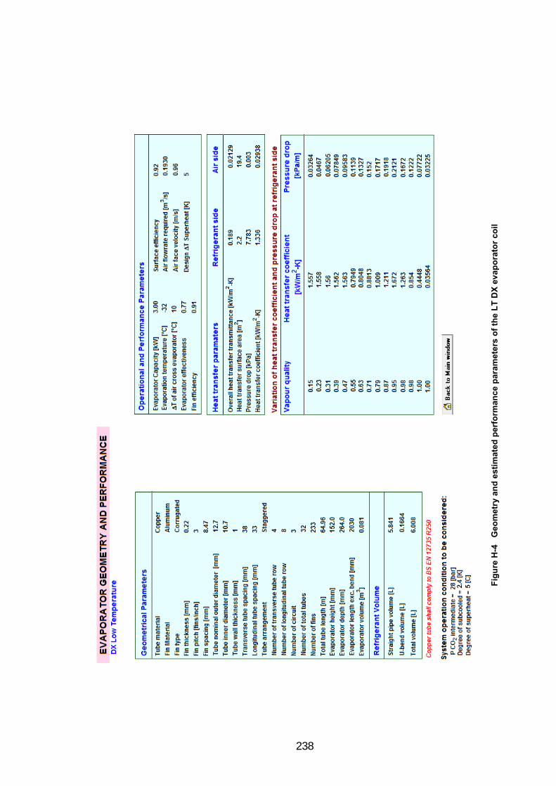
238

Fig

ure

H-4

G

eom

etry

an

d e

stim

ated

per

form

ance

par

amet

ers

of

the

LT

DX

eva

po

rato

r co

il

239

AAPPPPEENNDDIIXX II::

AAss bbuuiilltt iinntteeggrraatteedd ttrriiggeenneerraattiioonn aanndd CCOO22 rreeffrriiggeerraattiioonn

Abs

orpt

ion

unit

He

ade

r ta

nk

Dea

erat

or

Chi

lled

fluid

pu

mp

V=

Flo

w-r

ate

mea

sure

me

nt

T=

Te

mpe

ratu

re m

easu

rem

ent

Hot

flu

id

pum

p

Exh

aust

g

as

Flu

id

rece

ive

r

Exp

ansi

on

tank

P

= P

ress

ure

me

asu

rem

ent

V

T

T

P

Gen

erat

or

c/w

flu

id

jack

et

Inle

t air

Nat

ura

l gas

Rec

upe

rato

r

Air

Com

pres

sor

Mic

ro-

turb

ine

Com

-bu

sto

r

Boiler HX

Po

wer

Pla

nt

MT

Eva

p.

MT

Dis

pla

y ca

bin

et

LT

Dis

pla

y c

abin

et

LT

Eva

p.

m

m

Pu

lse

ves

sel

m=

Mas

s flo

w-r

ate

mea

sure

me

nt

Dry

bla

st

coo

ling

uni

t

Co

nden

ser

Sta

ndst

ill

con

dens

ing

unit

Com

pre

sso

r B

ock

HG

X12

P/6

0-4

CO

2 P

ump

CO

2 re

frig

era

nt

AK

V

IHX

Liq

uid

leve

l tr

ansm

itte

r

T

T

V

m

Fig

ure

I-1

S

chem

atic

dia

gra

m o

f th

e as

-bu

ilt t

est

faci

lity

240

AAPPPPEENNDDIIXX JJ::

UUnncceerrttaaiinnttyy aannaallyyssiiss

In the analysis of test results, key parameters such as: circulation ratio CR = 1 and

coefficient of performance (COP) are not directly measured. They are calculated as a

function of one or more variables that are directly measured. Each measured variable

has a random variability which is referred to as its “uncertainty”. This appendix

describes the calculations of uncertainty propagation of measured variables into the

calculated parameters which include: circulation ratio of 1, COP of the MT, LT and

COP of the overall CO2 refrigeration system. The uncertainty of reversed Carnot COP

calculation is also presented.

The uncertainty propagation was determined using the EES software with an

assumption that individual measurements are uncorrelated and random. In general,

uncertainty of the calculated parameters can be determined from (EES, 2010):

i

Xi

Y iU

X

YU 2

2

(J.1)

Where:

Y = calculated parameter; Xi = measured variables; UY = uncertainty of calculated

parameter; UXi = uncertainty of measured variables

J.1 Uncertainty of the calculation of the circulation ratio CR = 1

Circulation ratio is a function of measured variables as below:

CR = f ( MTrm , , TevapMT, RHa.ON, RHa.OFF, Ta.ON, Ta.OFF, L, w, va) (J.2)

Refers to equations (5.6), (5.7) and (5.8) in Chapter 5.

Where: MTrm , = MT refrigerant mass flow rate (kg/s); TevapMT = MT evaporating

temperature (oC); RHa.ON and RHa.OFF are relative humidity of air-on and air-off; Ta.ON

and Ta.OFF are temperature of air-on and off respectively (oC); L and w are sectional

dimensions of the air duct after the MT coil (m); va is air velocity at the measured

sectional area of the air duct (m/s).

241

Uncertainties of the measured variables for calculation uncertainty of the circulation

ratio CR = 1 are shown in Table J-1.

Table J-1 Uncertainties of the measured variables for calculation uncertainty of the circulation ratio CR = 1

Measured variable

Value at CR = 1

Unit Absolute

uncertainty Relative

uncertainty

MTrm , 0.019 kg/s 0.00035

TevapMT -7 oC 0.5

RHa.ON 0.76 - 0.015

RHa.OFF 0.91 - 0.015

Ta.ON 5 oC 0.5

Ta.OFF -3 oC 0.5

L 2.1 m 0.0005

w 0.04 m 0.0005

va 3.68 m/s 0.03

Uncertainty of L and w were assumed to be 0.5 mm The uncertainties of the measured variables refer to Section 3.6.1 (Chapter 3)

Results of the uncertainty analysis for the CR obtained from EES:

Uncertainty of the circulation ratio was determined to be

Absolute uncertainty: ± 0.111

Relative uncertainty: ± 10.8%

J.2 Uncertainty of the COP calculation

Coefficient of performance (COP) of the refrigeration system is a function of the

following measured variables:

COP = f ( MTrm , , LTrm , , PMT, PLT, Tevap.out.LT, Wcomp, WCO2pump) (J.2)

 

242

Uncertainties of the measured variables for the calculation of uncertainty of the COPs

are shown in Table J-2

Table J-2 Uncertainties of the measured variables for uncertainty of the COP calculations

Measured variable

Value

Unit Absolute

uncertainty Relative

uncertainty

CR 1.3 - 0.108

MTrm , 0.026 kg/s 0.00035

LTrm , 0.032 kg/s 0.00035

PLT 12.3 bar 0.03

PMT 27.8 bar 0.03

Tevap.out.LT -17 oC 0.5

Wcomp 2.55 kW 0.00036

WCO2pump 0.11 kW 0.00036

The uncertainties of the measured variables refer to Section 3.6.1 (Chapter 3)

Results of the uncertainty analysis for COP obtained using EES:

The uncertainty of the reversed Carnot COP

o Absolute uncertainty: ± 0.0526

o Relative uncertainty: ± 0.6%

Detailed results:

The uncertainty of the COPMT

o Absolute uncertainty: ± 4.921

o Relative uncertainty: ± 10.8%

 

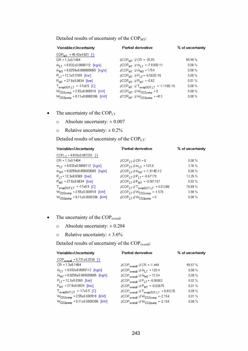
243

Detailed results of uncertainty of the COPMT:

The uncertainty of the COPLT

o Absolute uncertainty: ± 0.007

o Relative uncertainty: ± 0.2%

Detailed results of uncertainty of the COPLT:

The uncertainty of the COPoverall

o Absolute uncertainty: ± 0.204

o Relative uncertainty: ± 3.6%

Detailed results of uncertainty of the COPoverall:

  

 

 

244

AAPPPPEENNDDIIXX KK::

RReeffrriiggeerraanntt cchhaarrggee aanndd lleeaakk rraattee

This appendix presents a typical refrigerant charge for different sector of applications

and reported annual leak rate of different refrigeration equipment for the UK. This

appendix is related to Section 1.2 (Chapter 1) and Section 2.1 (Chapter 2).

Table K-1 Specific refrigerant charge for particular refrigeration system applications

Source: MTP, 2008

Table K-2 Reported annual leakage rates for particular refrigeration system applications in the UK

Source: MTP, 2008

245

AAPPPPEENNDDIIXX LL::

EEEESS MMooddeellss ooff tthhee rreeffrriiggeerraattiioonn ssyysstteemmss ffoorr tthhee ccoonnvveennttiioonnaall aanndd

ttrriiggeenneerraattiioonn –– CCOO22 rreeffrriiggeerraattiioonn eenneerrggyy ssyysstteemmss

Fig

ure

L-1

A

dis

pla

y o

f th

e E

ES

mo

del

fo

r th

e co

nve

nti

on

al s

up

erm

arke

t re

frig

erat

ion

sys

tem

usi

ng

R-4

04A

ref

rig

eran

t

246

Fig

ure

L-2

A

dis

pla

y o

f th

e E

ES

mo

del

fo

r th

e tr

ansc

riti

cal C

O2 r

efri

ger

atio

n c

asc

ad

ed w

ith

a t

rig

ener

atio

n s

yste

m o

f S

chem

e-2

(C

hap

ter

7)

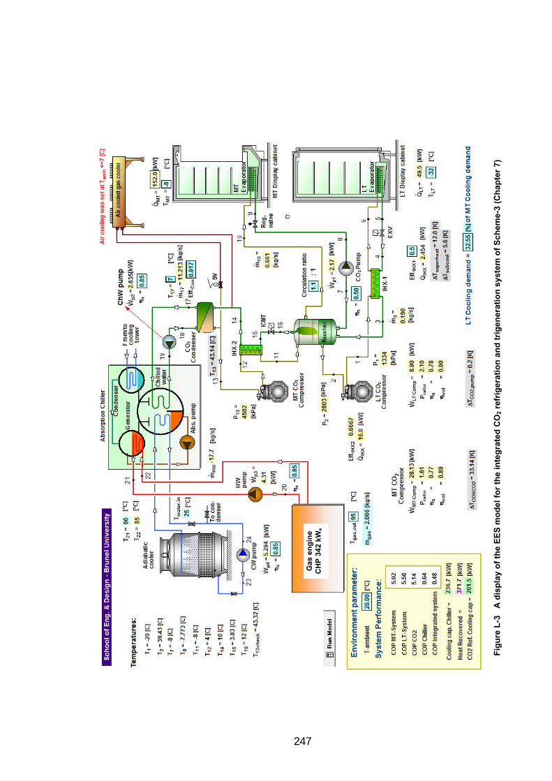
247

Fig

ure

L-3

A

dis

pla

y o

f th

e E

ES

mo

del

fo

r th

e in

teg

rate

d C

O2 r

efri

ger

atio

n a

nd

tri

gen

erat

ion

sys

tem

of

Sch

eme

-3 (

Ch

apte

r 7)

Gas

en

gin

e C

HP

342

kW

e

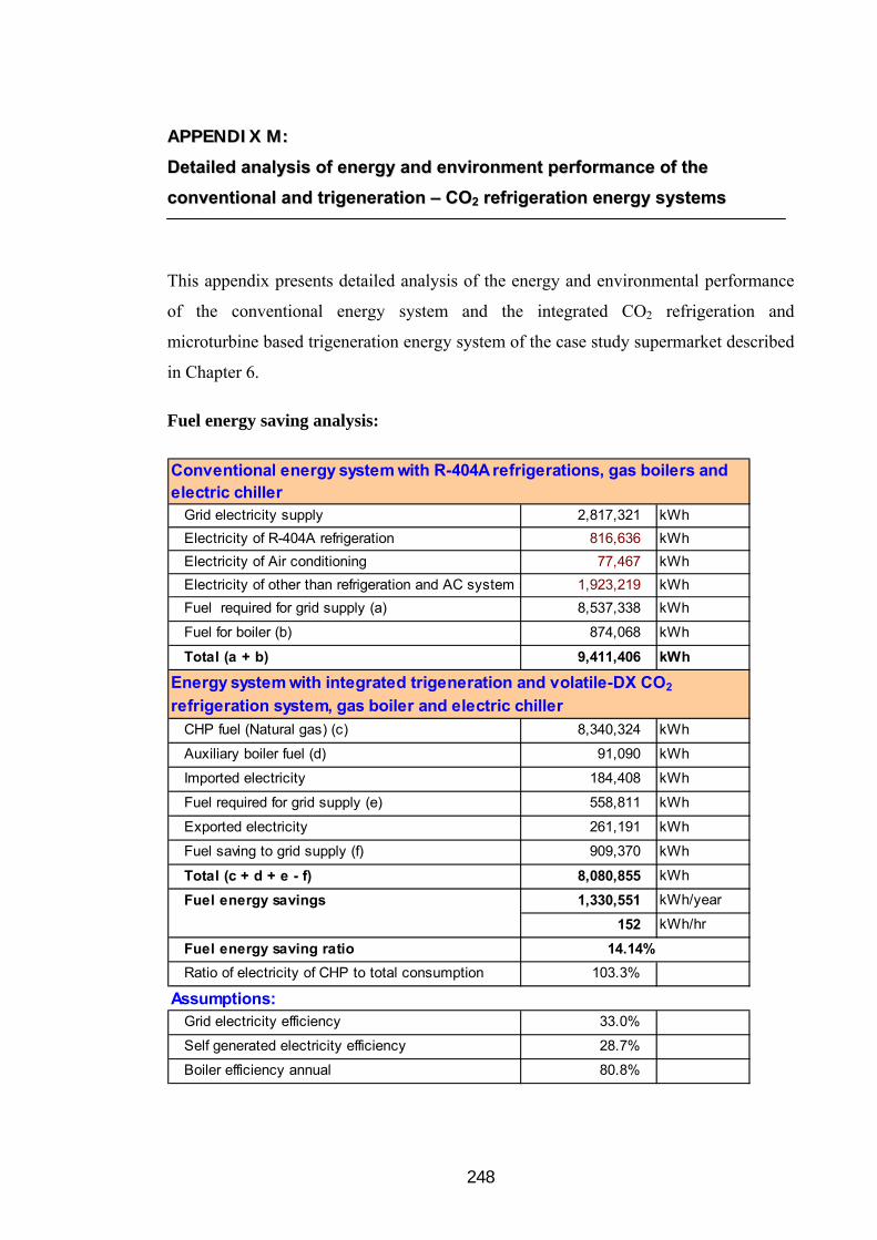
248

AAPPPPEENNDDIIXX MM::

DDeettaaiilleedd aannaallyyssiiss ooff eenneerrggyy aanndd eennvviirroonnmmeenntt ppeerrffoorrmmaannccee ooff tthhee

ccoonnvveennttiioonnaall aanndd ttrriiggeenneerraattiioonn –– CCOO22 rreeffrriiggeerraattiioonn eenneerrggyy ssyysstteemmss

This appendix presents detailed analysis of the energy and environmental performance

of the conventional energy system and the integrated CO2 refrigeration and

microturbine based trigeneration energy system of the case study supermarket described

in Chapter 6.

Fuel energy saving analysis:

Grid electricity supply 2,817,321 kWh

Electricity of R-404A refrigeration 816,636 kWh

Electricity of Air conditioning 77,467 kWh

Electricity of other than refrigeration and AC system s 1,923,219 kWh

Fuel required for grid supply (a) 8,537,338 kWh

Fuel for boiler (b) 874,068 kWh

Total (a + b) 9,411,406 kWh

CHP fuel (Natural gas) (c) 8,340,324 kWh

Auxiliary boiler fuel (d) 91,090 kWh

Imported electricity 184,408 kWh

Fuel required for grid supply (e) 558,811 kWh

Exported electricity 261,191 kWh

Fuel saving to grid supply (f) 909,370 kWh

Total (c + d + e - f) 8,080,855 kWh

Fuel energy savings 1,330,551 kWh/year

152 kWh/hr

Fuel energy saving ratio 14.14%

Ratio of electricity of CHP to total consumption 103.3%

Assumptions:Grid electricity efficiency 33.0%

Self generated electricity efficiency 28.7%

Boiler efficiency annual 80.8%

Energy system with integrated trigeneration and volatile-DX CO2

refrigeration system, gas boiler and electric chiller

Conventional energy system with R-404A refrigerations, gas boilers and electric chiller

249

CO2 emission analysis for Chapter 6:

Indirect CO2 emissions kWh kgCO2

Grid electricity consumption (A) 2,817,321 1,541,075

Natural gas consumption (B) 874,068 160,829

Direct CO2 emissions kg kgCO2

Annual R-404A refrigerant leakage ( C1) 105 411,443

Annual R-404A refrigerant recovery losses (D) 14 54,859

Annual R-407C refrigerant leakage (C2) 9 16,740

2,184,946

Indirect CO2 emissions kWh kgCO2

CHP fuel (F) 8,340,324 1,534,620

Boiler fuel (G) 91,090 16,761

Imported electricity (H) 184,408 100,871

Saving from exported electricity (I) 261,191 142,871

Total (K) = (F)+(G)+(H)-(I) 1,509,380

Direct CO2 emissions kg kgCO2

Annual refrigerant leakage of R-744 system (L) 53 53

Annual refrigerant leakage of the electric chiller R-407C (M) 9 16,740

Total (P) = (L)+(M) 16,793

1,526,173

658,773

30.15%

Net emission saving = (E)-(Q)

Percentage of the CO2 emission savings

Conventional energy system with R-404A refrigerations, gas boilers and electric chiller

Total (E) = (A)+(B)+(C1)+(D)+(C2)

Energy system with integrated trigeneration and volatile-DX CO2 refrigeration

system, gas boiler and electric chiller

Total (Q) = (K)+(P)

250

AAPPPPEENNDDIIXX NN::

DDeettaaiilleedd aannaallyyssiiss ooff eenneerrggyy aanndd eennvviirroonnmmeenntt ppeerrffoorrmmaannccee ooff tthhee eenneerrggyy

ssyysstteemm aalltteerrnnaattiivveess

This appendix details the energy and environment performance analysis of the energy

system alternatives of the case study supermarket. The analysis compares the

performance of the energy system alternatives to the conventional energy system with

R-404A refrigerant.

Fuel energy saving analysis of Scheme-1:

CHP fuel (Biodiesel) 4,430,848 kWh

Auxiliary boiler fuel 21,096 kWh

Imported electricity 1,159,933 kWh

Fuel required for grid supply 3,514,949 kWh

Exported electricity 120 kWh

Fuel saving to grid supply 364 kWh

Total 7,966,529 kWh

Fuel savings 1,444,877 kWh/year

165 kWh/hr

Fuel saving ratio 15.35%

Ratio of electricity of CHP to total consumption 57.3%

Assumptions:Grid electricity efficiency 33.0%

Self generated electricity efficiency 35.1%

Boiler efficiency annual 80.8%

Scheme-1

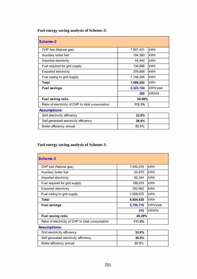
251

Fuel energy saving analysis of Scheme-2:

Fuel energy saving analysis of Scheme-3:

CHP fuel (Natural gas) 7,907,431 kWh

Auxiliary boiler fuel 194,360 kWh

Imported electricity 44,440 kWh

Fuel required for grid supply 134,666 kWh

Exported electricity 378,908 kWh

Fuel saving to grid supply 1,148,206 kWh

Total 7,088,252 kWh

Fuel savings 2,323,154 kWh/year

265 kWh/hr

Fuel saving ratio 24.68%

Ratio of electricity of CHP to total consumption 113.1%

Assumptions:Grid electricity efficiency 33.0%

Self generated electricity efficiency 36.6%

Boiler efficiency annual 80.8%

Scheme-2

CHP fuel (Natural gas) 7,450,016 kWh

Auxiliary boiler fuel 24,670 kWh

Imported electricity 62,343 kWh

Fuel required for grid supply 188,919 kWh

Exported electricity 332,962 kWh

Fuel saving to grid supply 1,008,975 kWh

Total 6,654,630 kWh

Fuel savings 2,756,776 kWh/year

315 kWh/hr

Fuel saving ratio 29.29%

Ratio of electricity of CHP to total consumption 111.0%

Assumptions:Grid electricity efficiency 33.0%

Self generated electricity efficiency 36.6%

Boiler efficiency annual 80.8%

Scheme-3

252

CO2 emission analysis of the energy system alternatives:

Indirect CO2 emissions kWh kgCO2

CHP fuel (F) 4,430,848 0

Boiler fuel (G) 21,096 3,882

Imported electricity (H) 1,159,933 634,483

Saving from exported electricity (I) 120 66

Total (K) = (F)+(G)+(H)-(I) 638,299

Direct CO2 emissions kg kgCO2

Annual refrigerant leakage of R-744 system (L) 53 53

Annual refrigerant leakage of electric chiller R-407C (M) 9 16,740

Total (P) = (L)+(M) 16,793

655,092

1,529,854

70.02%

Net emission savings = (E)-(Q)

Percentage of the CO2 emission savings

Scheme-1

Total (Q) = (K)+(P)

Indirect CO2 emissions kWh kgCO2

CHP fuel (F) 7,907,431 1,454,967

Boiler fuel (G) 194,360 35,762

Imported electricity (H) 44,440 24,309

Saving from exported electricity (I) 378,908 207,263

Total (K) = (F)+(G)+(H)-(I) 1,307,776

Direct CO2 emissions kg kgCO2

Annual refrigerant leakage of R-744 system (L) 53 53

Annual refrigerant leakage of electric chiller R-407C (M) 9 16,740

Total (P) = (L)+(M) 16,793

1,324,568

860,377

39.38%

Net emission savings = (E)-(Q)

Percentage of the CO2 emission savings

Scheme-2

Total (Q) = (K)+(P)

Indirect CO2 emissions kWh kgCO2

CHP fuel (F) 7,450,016 1,370,803

Boiler fuel (G) 24,670 4,539

Imported electricity (H) 62,343 34,102

Saving from exported electricity (I) 332,962 182,130

Total (K) = (F)+(G)+(H)-(I) 1,227,314

Direct CO2 emissions kg kgCO2

Annual refrigerant leakage of R-744 system (L) 53 53

Annual refrigerant leakage of electric chiller R-407C (M) 9 16,740

Total (P) = (L)+(M) 16,793

1,244,107

940,839

43.06%

Net emission savings = (E)-(Q)

Percentage of the CO2 emission savings

Scheme-3

Total (Q) = (K)+(P)

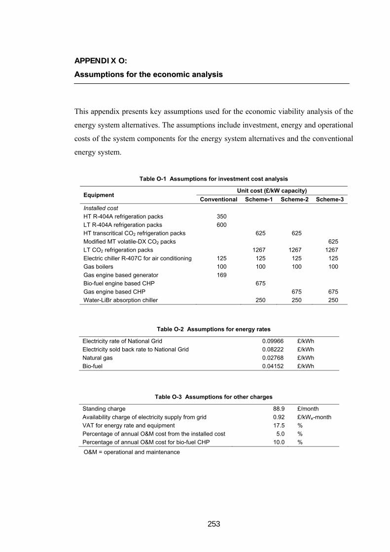
253

AAPPPPEENNDDIIXX OO::

AAssssuummppttiioonnss ffoorr tthhee eeccoonnoommiicc aannaallyyssiiss

This appendix presents key assumptions used for the economic viability analysis of the

energy system alternatives. The assumptions include investment, energy and operational

costs of the system components for the energy system alternatives and the conventional

energy system.

Table O-1 Assumptions for investment cost analysis

Equipment Unit cost (£/kW capacity)

Conventional Scheme-1 Scheme-2 Scheme-3

Installed cost

HT R-404A refrigeration packs 350

LT R-404A refrigeration packs 600

HT transcritical CO2 refrigeration packs 625 625

Modified MT volatile-DX CO2 packs 625

LT CO2 refrigeration packs 1267 1267 1267

Electric chiller R-407C for air conditioning 125 125 125 125

Gas boilers 100 100 100 100

Gas engine based generator 169

Bio-fuel engine based CHP 675

Gas engine based CHP 675 675

Water-LiBr absorption chiller 250 250 250

Table O-2 Assumptions for energy rates

Electricity rate of National Grid 0.09966 £/kWh

Electricity sold back rate to National Grid 0.08222 £/kWh

Natural gas 0.02768 £/kWh

Bio-fuel 0.04152 £/kWh

Table O-3 Assumptions for other charges

Standing charge 88.9 £/month

Availability charge of electricity supply from grid 0.92 £/kWe-month

VAT for energy rate and equipment 17.5 %

Percentage of annual O&M cost from the installed cost 5.0 %

Percentage of annual O&M cost for bio-fuel CHP 10.0 %

O&M = operational and maintenance