intellectual property statement - repository home

Copyright

by

Mintae Kim

2004

Intellectual Property Statement

“The software implementation of the Automated Multilevel Substructuring (AMLS)

method is a commercial product and much of the intellectual property related to

AMLS is protected by both copyrights and patents. Such protected technology may

include some or all of the material described herein. Please contact The Office of

Technology Commercialization at The University of Texas at Austin at 512.471.2995

or Professor Jeffrey K. Bennighof at 512.471.4709 if you are interested in licensing

or developing a commercial implementation of this technology.”

The Dissertation Committee for Mintae Kim

certifies that this is the approved version of the following dissertation:

An Efficient Eigensolution Method and Its

Implementation for Large Structural Systems

Committee:

Jeffrey K. Bennighof, Supervisor

Roy R. Craig, Jr.

Ronald O. Stearman

Leszek F. Demkowicz

Inderjit S. Dhillon



by

Mintae Kim, B.S., M.S.M.E.

Dissertation

Presented to the Faculty of the Graduate School of

The University of Texas at Austin

in Partial Fulfillment

of the Requirements

for the Degree of

Doctor of Philosophy


May 2004

UMI Number: 3143882

________________________________________________________ UMI Microform 3143882

Copyright 2004 by ProQuest Information and Learning Company.

All rights reserved. This microform edition is protected against

unauthorized copying under Title 17, United States Code.

____________________________________________________________

ProQuest Information and Learning Company 300 North Zeeb Road

PO Box 1346 Ann Arbor, MI 48106-1346

To my wife and family, especially to my father who passed away in 2001

Acknowledgments

First of all, I would like to express great gratitude to Dr. Bennighof for guiding me

to the academic and professional achievements of the great level. I have benefited

greatly from Dr. Bennighof’s expertise, passion, inspiration and encouragement.

Also, I would like to thank him for always providing constant support and numerous

suggestions and careful reading of this dissertation.

I would like to express my gratitude to my other four committee members. It

has been great honor for me to work with Dr. Craig, Dr. Stearmann, Dr. Demkowicz,

and Dr. Dhillon. I would like to thank Dr. Dhillon for providing his expertise on

dense eigenvalue problem and supporting his new tridiagonal eigensolver routine.

I would like to thank Matthew Kaplan for giving me an insight to initiate this

research. I am very grateful to Mark Muller, who always helps me to continuously

develop my programming skill in such a high level. Also, I am very grateful to

Chang-Wan Kim, Eric Swenson, Garrett Moran, Jeremiah Palmer, Tim Allison,

and Frederic Jottras in my office for providing me with numerous discussions and

suggestions. I am very grateful to Korean colleagues in Aerospace Engineering and

Engineering Mechanics, Soojae Park, Ungdai Ko, Sehyuk Im, Jaeyoung Lim, Kilho

Eom, Ike Lee, and other friends for their close support and encouragement. I am

very grateful to all my church friends who has been prayed for me. Without their

continuous support and prayers, I could not have achieved the goal of this research.

This research has been supported by Ford Motor Company, CDH GmbH,

v

IBM, Cray, SGI, Sun Micorsystems, Hewlett-Packard. I would like to express special

thank to Mladen Chargin in CDH GmbH for his support on this research. I would

like to thank Osni Marques, Doug Petesch, David Whitaker, Cheng Liao, and Mark

Kelly for sharing their knowledge.

Finally, I would like to praise and thank the LORD God for allowing me to

study and continuously guiding me to this level. I humbly confess that I would not

have been here without His great help and guidance. Whenever I get frustrated,

these words from the LORD God gives me a hope to recover.

Delight yourself in the LORD

and he will give you the desires of your heart.

Commit your way to the LORD;

trust in him and he will do this:

He will make your righteousness shine like the dawn,

the justice of your cause like the noonday sun.

Psalms 37:4-6

Mintae Kim


May 2004

vi



Publication No.

Mintae Kim, Ph.D.

The University of Texas at Austin, 2004

Supervisor: Jeffrey K. Bennighof

The automated multilevel substructuring (AMLS) method, which was originally

designed for efficient frequency response analysis, has emerged as an alternative to

the shift-invert block Lanczos method [23] for very large finite element (FE) model

eigenproblems. In AMLS, a FE model of a structure, typically having a ten mil-

lion degrees of freedom, is automatically and recursively divided into more than

ten thousand substructures on dozens of levels. This FE model is projected onto

the substructure eigenvector subspace which typically has a dimension of 100,000.

Solving the reduced eigenproblem on the substructure eigenvector subspace, how-

ever, is unmanageable for modally dense models which typically contain more than

10,000 eigenpairs. In this dissertation, a new eigensolution algorithm for the reduced

eigenproblem produced by the AMLS transformation is presented for large structural

systems with many eigenpairs. The new eigensolver in combination with AMLS is

advantageous for solving the eigenproblems for huge FE models with many eigen-

pairs because it takes much less computer time and resource than any other existing

eigensolvers while maintaining acceptable eigensolution accuracy. Therefore, the

vii

new eigensolution algorithm not only makes high frequency analysis possible with

acceptable accuracy, but also extends the capability of solving large scale eigenvalue

problems requiring many eigenpairs.

A reduced eigenvalue problem produced by the AMLS transformation for a

large finite element model is defined on the substructure eigenvector subspace. A

new distilled subspace is obtained by defining subtrees in the substructure tree,

solving subtree eigenproblems, and truncating subtree and branch substructure

eigenspaces. Then the reduced eigenvalue problem on the substructure eigenvec-

tor subspace is projected onto the smaller distilled subspace, utilizing the sparsity

of the stiffness and mass matrices. Using a good guess of a starting subspace on

the distilled subspace, which is represented by a sparse matrix, one subspace it-

eration recovers as much accuracy as needed. Hence, the size of the eigenvalue

problem for Rayleigh-Ritz analysis can be greatly minimized. Approximate global

eigenvalues are obtained by solving the Rayleigh-Ritz eigenproblem on the refined

subspace, computed by one subspace iteration, and the corresponding eigenvectors

are recovered by simple matrix-matrix multiplications.

For robustness of the implementation of the new eigensolution algorithm,

the remedies for a nearly singular stiffness matrix and an indefinite mass matrix are

presented. Also, the new eigensolution algorithm is very parallelizable. The parallel

implementation of this new eigensolution algorithm for shared memory multipro-

cessor machines is done by using OpenMP Application Program Interface (API) for

performance improvement. Timing and eigensolution accuracy of the implementa-

tion of the new eigensolution algorithm are presented, compared with the results

from the block Lanczos eigensolver in the commercial software MSC.Nastran. In

addition to the new eigensolution algorithm, a new method for an augmented eigen-

problem for residual flexibility is developed to mitigate loss of accuracy by paying

little computational cost in modal frequency response analysis.

viii

Contents

Acknowledgments v

Abstract vii

List of Tables xii

List of Figures xv

Chapter 1 Introduction 1

1.1 Challenges and Motivations . . . . . . . . . . . . . . . . . . . . . . . 3

1.2 Overview of AMLS Software . . . . . . . . . . . . . . . . . . . . . . . 5

1.3 Outline of Dissertation . . . . . . . . . . . . . . . . . . . . . . . . . . 6

Chapter 2 Reduced Eigenproblem by the AMLS Transformation 9

2.1 Reduced Eigenvalue Problem . . . . . . . . . . . . . . . . . . . . . . 9

2.2 An Overview of the AMLS Transformation . . . . . . . . . . . . . . 11

Chapter 3 Survey of Eigensolution Methods 22

3.1 Single Vector Iteration Methods . . . . . . . . . . . . . . . . . . . . . 23

3.2 Subspace Iteration Methods . . . . . . . . . . . . . . . . . . . . . . . 25

3.3 Lanczos Methods . . . . . . . . . . . . . . . . . . . . . . . . . . . . . 28

3.4 Similarity Transformation Methods . . . . . . . . . . . . . . . . . . . 33

ix

Chapter 4 A New Eigensolution Algorithm 35

4.1 Motivation for a New Eigensolution Algorithm . . . . . . . . . . . . 35

4.1.1 Reduced Eigenproblem Characteristics . . . . . . . . . . . . . 36

4.1.2 Lanczos Method versus Subspace Iteration Method . . . . . . 37

4.2 Preliminary Eigensolution Algorithm . . . . . . . . . . . . . . . . . . 40

4.3 Projection onto a Distilled Subspace . . . . . . . . . . . . . . . . . . 42

4.4 Starting Subspace . . . . . . . . . . . . . . . . . . . . . . . . . . . . 52

4.5 Subspace Improved by One “Inverse Iteration” . . . . . . . . . . . . 55

4.6 Rayleigh-Ritz Analysis . . . . . . . . . . . . . . . . . . . . . . . . . . 56

4.7 Computation of Eigenvectors on the Subspace A . . . . . . . . . . . 59

4.8 Practical Issues in Numerical Implementation . . . . . . . . . . . . . 59

4.8.1 Low Frequency Modes . . . . . . . . . . . . . . . . . . . . . . 60

4.8.2 Indefinite Mass Matrix . . . . . . . . . . . . . . . . . . . . . . 62

Chapter 5 Parallel Implementation of the New Algorithm 64

5.1 Parallelism for Projection onto the Distilled Subspace . . . . . . . . 66

5.2 Parallelism for Rayleigh-Ritz Analysis . . . . . . . . . . . . . . . . . 70

5.2.1 Parallelism for Projecting the Eigenproblem onto Ritz Subspace 71

5.2.2 Parallelism for Solving the Projected Eigenproblem on Ritz

Subspace . . . . . . . . . . . . . . . . . . . . . . . . . . . . . 73

5.2.3 Parallelism for Computing the Ritz Eigenvectors . . . . . . . 76

5.3 Parallelism for Computing Approximate Eigenvectors on the Sub-

space A . . . . . . . . . . . . . . . . . . . . . . . . . . . . . . . . . . 78

Chapter 6 Numerical Results and Performance 81

6.1 Trim-Body Model . . . . . . . . . . . . . . . . . . . . . . . . . . . . . 86

6.1.1 Effect of Maximum Subtree Size . . . . . . . . . . . . . . . . 88

6.1.2 Effect of the Distillation Cutoff Frequency . . . . . . . . . . . 91

x

6.1.3 Effect of Starting Subspace Cutoff Frequencies . . . . . . . . 94

6.1.4 Parallel Performance . . . . . . . . . . . . . . . . . . . . . . . 98

6.1.5 Overall Performance and Eigensolution Accuracy . . . . . . . 100

6.2 Full-Vehicle Model . . . . . . . . . . . . . . . . . . . . . . . . . . . . 105

6.2.1 Effect of Maximum Subtree Size . . . . . . . . . . . . . . . . 107

6.2.2 Effect of the Distillation Cutoff Frequency . . . . . . . . . . . 109

6.2.3 Effect of Starting Subspace Cutoff Frequencies . . . . . . . . 111

6.2.4 Parallel Performance . . . . . . . . . . . . . . . . . . . . . . . 116

6.2.5 Overall Performance and Eigensolution Accuracy . . . . . . . 118

6.3 8.4M DOF Model . . . . . . . . . . . . . . . . . . . . . . . . . . . . . 122

6.3.1 Phase4 Performance . . . . . . . . . . . . . . . . . . . . . . . 124

6.3.2 Eigensolution Accuracy of Phase4 . . . . . . . . . . . . . . . 125

6.3.3 Parallel Performance of Phase4 . . . . . . . . . . . . . . . . . 126

6.4 Summary of Numerical Results . . . . . . . . . . . . . . . . . . . . . 128

Chapter 7 Conclusions and Future Work 130

7.1 Conclusions . . . . . . . . . . . . . . . . . . . . . . . . . . . . . . . . 130

7.2 Future Work . . . . . . . . . . . . . . . . . . . . . . . . . . . . . . . 133

7.3 Final Remarks . . . . . . . . . . . . . . . . . . . . . . . . . . . . . . 134

Appendix A Augmented Eigenproblem for Residual Flexibility 136

A.1 Residual Flexibility and Block Orthogonalization . . . . . . . . . . . 137

A.2 Preliminary Residual Flexibility Eigensolution Algorithm . . . . . . 138

A.3 Block Orthogonalization Procedure . . . . . . . . . . . . . . . . . . . 140

A.4 Small Eigenproblem for Residual Flexibility . . . . . . . . . . . . . . 142

Bibliography 145

Vita 154

xi

List of Tables

4.1 The number of natural frequencies in several frequency ranges for

“8.4M DOF” model . . . . . . . . . . . . . . . . . . . . . . . . . . . 38

5.1 Sequential performance of the new algorithm implementation for “Full-

Vehicle” model. . . . . . . . . . . . . . . . . . . . . . . . . . . . . . . 66

6.1 Phase2 and Phase3 performance for Trim-Body model . . . . . . . . 87

6.2 Effect of maximum subtree size on the dimension and quality of the

distilled subspace D for Trim-Body model . . . . . . . . . . . . . . . 88

6.3 Effect of maximum subtree size on the eigensolution accuracy and

performance of Phase4 for Trim-Body model . . . . . . . . . . . . . 89

6.4 Effect of the distillation cutoff frequency ωD for Trim-Body model . 92

6.5 Effect of starting subspace cutoff frequency ωst

Vfor subtrees for Trim-

Body model . . . . . . . . . . . . . . . . . . . . . . . . . . . . . . . . 95

6.6 Effect of starting subspace cutoff frequency ωbs

Vfor branch substruc-

tures for Trim-Body model . . . . . . . . . . . . . . . . . . . . . . . 97

6.7 Parallel performance of Phase4 for Trim-Body model . . . . . . . . 98

6.8 Timings and speedups for parallelized steps in the new eigensolution

algorithm for Trim-Body model . . . . . . . . . . . . . . . . . . . . . 99

xii

6.9 Timings and speedups of Rayleigh-Ritz analysis in the new algorithm

for Trim-Body model . . . . . . . . . . . . . . . . . . . . . . . . . . . 99

6.10 Performance comparison between Phase4 and two other algorithms

on the different subspaces for Trim-Body model . . . . . . . . . . . 101

6.11 Phase2 and Phase3 performance for Full-Vehicle model . . . . . . . 106

6.12 Effect of maximum subtree size on the dimension and quality of the

distilled subspace D for Full-Vehicle model . . . . . . . . . . . . . . 108

6.13 Effect of maximum subtree size on the eigensolution accuracy and

performance of Phase4 for Full-Vehicle model . . . . . . . . . . . . . 108

6.14 Effect of the distillation cutoff frequency ωD for Full-Vehicle model . 111


Vfor subtrees on the

eigensolution accuracy and performance of Phase4 for Full-Vehicle

model . . . . . . . . . . . . . . . . . . . . . . . . . . . . . . . . . . . 113



tures on the performance and eigensolution accuracy of Phase4 for

Full-Vehicle model . . . . . . . . . . . . . . . . . . . . . . . . . . . . 114

6.17 Parallel Performance of the new eigensolution algorithm implemen-

tation for Full-Vehicle model . . . . . . . . . . . . . . . . . . . . . . 116

6.18 Timings and speedups for parallelized steps in the new eigensolution

algorithm for Full-Vehicle model . . . . . . . . . . . . . . . . . . . . 116

6.19 Timings and speedups of the Rayleigh-Ritz analysis in the new eigen-

solution algorithm for Full-Vehicle model . . . . . . . . . . . . . . . . 117

6.20 Performance comparison of Phase4 with the block Lanczos eigen-

solver on two different subspaces for Full-Vehicle model . . . . . . . 119

6.21 Overall performance of the AMLS software for 8.4M DOF model . . 123

6.22 Performance comparison between Phase4 and the block Lanczos eigen-

solver on the distilled subspace for 8.4M DOF model . . . . . . . . . 124

xiii

6.23 Parallel Performance of the new eigensolution algorithm for 8.4M

DOF model . . . . . . . . . . . . . . . . . . . . . . . . . . . . . . . . 127

6.24 Timings and speedups of Rayleigh-Ritz analysis in the new eigenso-

lution algorithm for 8.4M DOF model . . . . . . . . . . . . . . . . . 127

xiv

List of Figures

1.1 Flowchart of the AMLS software . . . . . . . . . . . . . . . . . . . . 7

2.1 (a) A square plate recursively partitioned to two levels. (b) Substruc-

ture tree associated with the two level partitioning. . . . . . . . . . . 12

3.1 Basic algorithm for inverse iteration method . . . . . . . . . . . . . . 24

3.2 Basic subspace iteration method for generalized eigenproblem . . . . 27

3.3 Basic Lanczos algorithm for generalized symmetric eigenproblem . . 30

3.4 Lanczos Loop for the block Lanczos algorithm . . . . . . . . . . . . . 31

4.1 New eigensolution algorithm for the reduced eigenproblem produced

by the AMLS transformation . . . . . . . . . . . . . . . . . . . . . . 40

4.2 Subspaces of the new eigensolution method . . . . . . . . . . . . . . 42

4.3 Effect of leaf substructure size for “Trim-Body” model . . . . . . . . 44

4.4 Substructure tree versus truncated substructure tree at subtree levels

for Trim-Body model . . . . . . . . . . . . . . . . . . . . . . . . . . . 45

4.5 Substructure tree truncation process. (a) Defining subtrees in the

original substructure tree. (b) Truncated substructure tree after

defining subtrees and truncating subtree eigenspace. . . . . . . . . . 46

4.6 Algorithm for Rayleigh-Ritz analysis on the Ritz subspace V1 . . . . 58

xv

5.1 Parallel algorithm for building TD implicitly and projecting KA and

MA onto the distilled subspace D . . . . . . . . . . . . . . . . . . . . 67

5.2 Dynamic scheduling and efficient ordering examples for paralleliza-

tion of subtree eigenproblems. (a) Efficient ordering with dynamic

scheduling. (b) Inefficient ordering with dynamic scheduling. . . . . 69

5.3 Parallel algorithm for projecting the mass matrix MD onto the Ritz

subspace V1 in Rayleigh-Ritz analysis . . . . . . . . . . . . . . . . . 71

5.4 Parallel block Cholesky factorization algorithm for MV = UT U . . . 74

5.5 Parallel block algorithm for forming AV = U−T KV U−1 . . . . . . . 75

5.6 Parallel algorithm for computing Ritz eigenvectors in Rayleigh-Ritz

analysis . . . . . . . . . . . . . . . . . . . . . . . . . . . . . . . . . . 77

5.7 Parallel algorithm for computing approximate eigenvectors on the

substructure eigenvector subspace (A) . . . . . . . . . . . . . . . . . 79

6.1 Finite element representation of Trim-Body model . . . . . . . . . . 85

6.2 Effect of maximum subtree size on the accuracy of the natural fre-

quencies by Phase4 for Trim-Body model . . . . . . . . . . . . . . . 91

6.3 Effect of the distillation cutoff frequency ωD on the accuracy of the

approximate natural frequencies for Trim-Body model . . . . . . . . 93



accuracy of the approximate natural frequencies for Trim-Body model 95



tures on relative errors of the approximate natural frequencies for

Trim-Body model . . . . . . . . . . . . . . . . . . . . . . . . . . . . . 97

6.6 Accuracy of the approximate natural frequencies by three different

algorithms on two different subspaces with the same global cutoff

frequency 600 Hz for Trim-Body model . . . . . . . . . . . . . . . . 102

xvi

6.7 Cosines of the principal angles between two eigenspaces computed by

Phase4 and the Lanczos eigensolver for Trim-Body model . . . . . . 104

6.8 Finite Element Representation of Full-Vehicle Model . . . . . . . . . 105

6.9 Effect of the maximum subtree size on the accuracy of the natural

frequencies computed by Phase4 for Full-Vehicle model . . . . . . . 110

6.10 Effect of distillation cutoff frequency ωD on accuracy of the approxi-

mate natural frequencies by Phase4 for Full-Vehicle model . . . . . . 112



accuracy of Phase4 for Full-Vehicle model . . . . . . . . . . . . . . . 113



tures on the accuracy of the natural frequencies computed by Phase4

for Full-Vehicle model . . . . . . . . . . . . . . . . . . . . . . . . . . 114

6.13 Accuracy of the natural frequencies computed by Phase4 and the

block Lanczos eigensolver on the distilled subspace (D) for Full-

Vehicle model . . . . . . . . . . . . . . . . . . . . . . . . . . . . . . . 119

6.14 Cosine of the principal angles between two eigenspaces computed by

Phase4 and the block Lanczos eigensolver on the subspace A for Full-

Vehicle model . . . . . . . . . . . . . . . . . . . . . . . . . . . . . . . 121

6.15 Accuracy of the approximate natural frequencies computed by Phase4

compared to the natural frequencies approximated by the block Lanc-

zos eigensolver on the distilled subspace for 8.4M DOF model. . . . 126

A.1 New augmented eigensolution algorithm for residual flexibility eigen-

solution . . . . . . . . . . . . . . . . . . . . . . . . . . . . . . . . . . 139

A.2 Algorithm for computing U in the block modified Gram-Schmidt or-

thogonalization . . . . . . . . . . . . . . . . . . . . . . . . . . . . . . 141

A.3 More efficient algorithm for computing U in the block modified Gram-

Schmidt orthogonalization . . . . . . . . . . . . . . . . . . . . . . . . 141

xvii

Chapter 1

Introduction

One of the main goals in structural dynamic analysis is to calculate the natural

frequencies and the corresponding natural modes of vibration of a structural system.

This leads to a generalized eigenvalue problem for the structure of the form

Kφ = ω2Mφ (1.1)

where K and M are n × n stiffness and mass matrices, respectively, ω is a natural

frequency and φ represents the corresponding natural mode of vibration for the

structure.

Aircraft, submarines, automobiles, complex machine components, and framed

structures are examples of structures that require efficient eigensolution techniques

for their dynamic analysis. Many of these structures are represented by finite ele-

ment (FE) models having millions of degrees of freedom. Engineers, especially in the

automotive industry, need to perform dynamic analysis to higher frequencies with

good accuracy and less computer time. This means that a more refined mesh is

required in a finite element model for accuracy especially at higher frequencies, and

the computational cost of the eigensolution has to decrease to make the dynamic

analysis feasible. These requirements are beyond the capabilities of conventional

1

eigensolution methods.

A classical approach for approximating the partial solution of large eigen-

problems consists of projecting the eigenproblem onto an approximating subspace

to reduce the computational cost of the eigensolution [56, 57, 58, 59, 60, 61]. The

automated multilevel substructuring (AMLS) method is an efficient dimensional

reduction tool that has recently been developed and is now widely used in the au-

tomotive industry [3, 4, 5, 6, 7].

In the AMLS method, a finite element model of a structure is automatically

and recursively divided into thousands of substructures on numerous levels. The

eigenspace of each substructure is truncated for dimensional reduction, and the

eigenvectors associated with these substructures are used to approximate the partial

eigensolution of the FE model. The global eigenvalue problem in the FE space is

projected onto the substructure eigenvector subspace. The size of the eigenproblem

after reduction, however, is still unmanageable for very large structural models

excited over a broad frequency range, and large computational resources are required

for even the reduced eigenvalue problem. Typically industrial models have millions

of degrees of freedom, and the reduced models produced by AMLS can have about

one hundred thousand degrees of freedom. For the reduced eigenvalue problem, the

required number of eigenpairs might be over ten thousand.

The goal of this dissertation is to develop an efficient eigensolution technique

for the reduced problem encountered in AMLS that improves performance in terms

of execution time, accuracy, storage requirements and robustness. A computer im-

plementation for a new algorithm must be efficient, so that not only is performance

improved but the capability of solving larger eigenvalue problems is extended by

minimizing the usage of computer resources.

2

1.1 Challenges and Motivations

In the modal dynamic analysis of complex structures, such as modal frequency re-

sponse analysis and modal transient response analysis, the main computational cost

is for calculating the required natural frequencies and natural modes of the struc-

ture. Much attention has been directed toward effective eigensolution techniques

for large eigenproblems. Since solving for the required natural frequencies and nat-

ural modes can be prohibitively expensive with conventional techniques when the

order of the structural system is large, approximate solution techniques have been

developed for finding the lowest eigenpairs.

There have been several competitors in approximate eigensolution techniques

for large scale structural systems, including the “shifted-invert” block Lanczos method

[23, 24], component mode synthesis methods [57, 58, 59, 60, 61], and the automated

multilevel substructuring method [1, 8]. Over the past 15 years or so, the block

Lanczos method has been dominant in the scientific and engineering areas as a

partial eigensolution method for large sparse eigenproblems, in conjunction with a

sparse direct (out-of-core) solver. However, the block Lanczos method has several

drawbacks in terms of computational performance [6]:

Requirement of High Memory Bandwidth

To get the high performance on the machines that has hierarchical memory sys-

tem, like most of microprocessor-based systems, it is important to reuse data

at the top of the memory hierarchy (vector register and cache memory) and

minimize the data movements. One way of measuring this data management is

the ratio of arithmetic operations to memory references [55, 71, 72]. The block

Lanczos algorithm has a very low ratio of arithmetic operations to memory

references, so that it requires a computer that has a high memory bandwidth

to keep processors supplied with data. As a result, vector supercomputers

have proven to be much faster for this algorithm than microprocessor-based

3

systems.

Significant I/O Requirement for Models with High Modal Density

Large amounts of data must be read from or written to disk, and this causes

problems if the CPU(s) must wait for the data transfer to finish. Since the

block Lanczos method is highly dependent upon large amounts of I/O for

models with high modal density (many closely spaced eigenvalues), the I/O

can result in a performance bottleneck.

Difficulty in Parallelization

Parallelization of the block Lanczos method has not been very successful for

FE models of very large size. To overcome this defect, one parallel Lanczos

scheme divides the frequency range among processors so the number of fre-

quencies in each segment is about equal. The Lanczos eigensolver then solves

the eigenproblem within each subrange of the frequency range on each pro-

cessor. However, this parallel scheme requires each processor to work on the

same full model and so memory and disk requirements for parallel run increase

as a multiple of the number of processors used. Therefore, the parallel Lanc-

zos eigensolver cannot complete the analysis due to the lack of computational

resources when FE models are very large and have high modal density.

The automated multilevel substructuring (AMLS) method, which was origi-

nally designed for efficient frequency response analysis, has emerged as an alternative

to the block Lanczos method for very large FE model eigenproblems. The AMLS

method requires far less memory bandwidth and fewer floating point operations

than the block Lanczos method [1, 6], because all the necessary computations are

done on the smaller substructure eigenvector subspace than large FE degrees of

freedom, and also only one numerical pass through K and M data, rather than

many factorizations and out of core solves, and multiplications. The AMLS method

has much less data transfer than the block Lanczos method, because in the block

4

Lanczos method, tens of thousands of eigenvectors and iteration vectors, expressed

in all of the FE degrees of freedom, must be read from or written out to disk for

iterations. In contrast, in AMLS it is not necessary to produce eigenvectors in all

FE degrees of freedom. As a result, large FE models can be analyzed with much less

data transfer, rather than tens of terabytes of data transfer required in the block

Lanczos method. The AMLS method is also inherently more parallelizable than the

block Lanczos algorithm. Different substructures can be processed simultaneously

and independently. Also, as transformation of the FE model to the substructure

eigenvector representation progresses toward the root of the substructure tree, there

is more opportunity for parallelizing the computation associated with each individ-

ual substructure [2, 6]. Therefore, the AMLS method has better capabilities than

the block Lanczos method for very large FE models.

However, the AMLS method has a significant bottleneck for modally dense

models in solving the reduced eigenproblem encountered in the AMLS method, as

mentioned by Kaplan [1]. For a trim body model from industry, as an example, he

showed that the overall performance of AMLS was governed by the performance of

the eigensolution process on the substructure eigenvector subspace. More specifi-

cally, the executable in the AMLS software that computes the eigensolution for the

reduced eigenproblem took about 75 % of the total elapsed time of AMLS, and this

executable determined the maximum memory usage and the maximum disk usage

for AMLS. The above challenges have served as the motivations for this disserta-

tion. Therefore, we want to develop an efficient and parallelizable algorithm and its

implementation for the reduced eigenproblem encountered in AMLS.

1.2 Overview of AMLS Software

The AMLS software for solving large sparse algebraic eigenproblems consists of four

separate programs [1]. Each program is responsible for one phase of the process. We

5

will denote the programs as Phase2, Phase3, Phase4, and Phase5. For convenience,

we refer to any FE software that generates FE matrices for AMLS as Phase1. There

is another phase for solving frequency response problems, which is called Phase6,

but this phase is not related to the scope of this dissertation. The flow of AMLS

software is outlined in Figure 1.1.

Phase1 generates FE model data, which include stiffness and mass matri-

ces, by some finite element software. In this dissertation, MSC.Nastran is the finite

element software package used to generate the finite element data. Phase2 reads

through the matrix data and automatically divides the FE model into thousands

of substructures on dozens of levels based on the sparsity structure of system ma-

trices. Phase3 computes hundred thousands of substructure eigenvectors whose

eigenvalues are below a specified cutoff value, which is much higher than the square

of the highest excitation frequency of interest, and projects the stiffness and mass

matrices onto the substructure eigenvector subspace. In Phase4, which contains

new eigensolution algorithm which is the focus of this dissertation, the global eigen-

solution is approximated. Phase5 computes the approximate eigenvectors on the

FE discretization subspace. This dissertation is focused on the new eigensolution

algorithm in Phase4 for the reduced eigenproblem on the substructure eigenvector

subspace and its implementation.

1.3 Outline of Dissertation

In this dissertation, we present an efficient numerical method for solving the symmet-

ric semi-definite generalized eigenvalue problem for large structural systems. The

following summarizes the outline of this dissertation.

In Chapter 2, the global eigenvalue problem is defined in the FE discretization

subspace. Since AMLS is used for model reduction, the AMLS transformation

process is explained briefly using a simple plate example. The reduced eigenvalue

6

Eigenanalysis Starts

Eigenanalysis Ends

Generate FE matrices( FE package )

Phase 1

Compute Eigenvectors

Phase 5

Define Substructure Tree

Phase 2

Solve Reduced Eigenproblem

Phase 4

Transform Model

Phase 3

AMLS

Figure 1.1: Flowchart of the AMLS software

7

problem generated by the AMLS transformation is defined. This reduced eigenvalue

problem is the one that we want to solve very efficiently using a new eigensolution

algorithm.

In Chapter 3, we discuss the existing algorithms available for solving the re-

duced eigenproblem, which is rather large and sparse. Since an eigensolver for dense

matrices is needed for Rayleigh-Ritz analysis for a new eigensolution algorithm, we

also discuss the stable and fast dense eigensolver for the standard eigenproblem,

which is obtained from the generalized eigenproblem by using a Cholesky factoriza-

tion of one of the matrices.

In Chapter 4, we describe the characteristics of the reduced eigenvalue prob-

lem in detail and the motivations for developing a new eigensolution algorithm.

Then, the new eigensolution algorithm for the reduced eigenproblem is explained in

detail. Two significant difficulties in implementing the new algorithm are discussed

with their remedies.

In Chapter 5, parallelization issues for the new algorithm are discussed for

shared memory multiprocessor machines.

In Chapter 6, numerical results are shown for three industrial models to show

the efficiency and accuracy of the new eigensolution algorithm.

In Chapter 7, we finish by summing up the conclusions of this dissertation

and highlighting areas of potential future work.

In addition to the above chapters, the augmented eigenvalue problem is dis-

cussed in Appendix A, to obtain the residual flexibility vectors for mitigating loss

of accuracy in frequency response analysis. A very cost efficient algorithm for the

large augmented eigenproblem for residual flexibility is described.

8

Chapter 2

Reduced Eigenproblem by the

AMLS Transformation

In this chapter, we will start from the generalized eigenvalue problem for a FE

model and proceed to define the reduced eigenproblem produced by the AMLS

transformation, giving a typical size of the problem. To help readers interested in

the AMLS transformation process, an overview of the AMLS transformation will be

presented with a simple plate example.

2.1 Reduced Eigenvalue Problem

The eigenvalue problem for the finite element model of a large scale structural system

is represented by the equation

K Φ = M Φ Λ (2.1)

where K ∈ RnF×nF and M ∈ R

nF×nF are finite element stiffness and mass matrices

which are real, symmetric, and positive semi-definite, and nF is the number of

degrees of freedom in the finite element model, which defines the dimension of the

9

problem. The matrix Λ ∈ RnE×nE is a diagonal matrix of the eigenvalues less than

a global cutoff value ωG

2, where nE is the number of global eigenpairs computed and

ωG is the global radian cutoff frequency for this eigenproblem, which is typically 50%

higher than the highest excitation frequency. The matrix Φ ∈ RnF×nE contains the

corresponding eigenvectors. We will assume that the eigenvalues are in increasing

order and the eigenvectors are normalized with respect to the mass matrix so that

ΦT MΦ = I, where I is an identity matrix.

The natural frequencies and modes of vibration of the structure can be ap-

proximated by solving this very large algebraic eigenproblem. The eigenvalues are

squares of natural frequencies and the eigenvectors represent natural modes of vibra-

tion. The system matrices, K and M , are sparsely populated and their dimension

is in the millions, so conventional eigensolution techniques are very costly.

To reduce the computational cost of the eigensolution, this global eigenprob-

lem can be projected onto an approximating subspace, which has a much smaller

dimension. With AMLS, the eigensolution is approximated using a subspace of sub-

structure eigenvectors [1, 11, 10] which can be produced very efficiently. By forming

the triple products,

KA = T TA K TA MA = T T

A M TA, (2.2)

where TA ∈ RnF×nA is an AMLS transformation matrix containing substructure

eigenvectors and nA is the total number of substructure eigenvectors computed, the

global eigenproblem is transformed to the form

KA ΦA = MA ΦA ΛA (2.3)

where ΦA ∈ RnA×nE is a matrix of eigenvectors and ΛA ∈ R

nE×nE is a diagonal

matrix containing eigenvalues for the reduced eigenproblem. The approximation of

the global eigensolution is given by Φ ≈ TAΦA and Λ ≈ ΛA.

10

The reduced eigenvalue problem is still not feasible to solve within a suit-

able job turn-around time on workstations using available eigensolution methods

because its dimension is typically on the order of one hundred thousand and the

required number of eigenpairs can be over ten thousand. This eigenvalue problem

is too large for a conventional eigensolver suited for dense problems, which typi-

cally uses Householder reduction to tridiagonalize the matrix, solves the tridiagonal

eigenproblem and backtransforms the solution of the tridiagonal eigenproblem to

the original space. In addition, the Lanczos method, which is ideal for finding a

few extreme eigenpairs for a sparse problem, does not perform well when so many

eigenpairs must be found.

The generalized eigenvalue problem in Equation (2.3) is the eigenproblem

that we are aiming to solve for the smallest nE (perhaps 10, 000) eigenvalues and

the corresponding eigenvectors. The new eigensolution approximation scheme for

this problem will be discussed in Chapter 4. In the next section, the AMLS trans-

formation is discussed in detail.

2.2 An Overview of the AMLS Transformation

In the AMLS method, a FE model of a structure is automatically divided into

two substructures, and then each of these is subdivided into its own substructures.

Here, a substructure is defined as a set of degrees of freedom in a finite element

model, which are typically associated with a group of contiguous finite elements.

This subdivision process is repeated recursively until substructures reach a specified

target size, so that typically ten thousands of substructures are defined on dozens

of levels.

For a simple illustrative example, consider a finite element model of a square

plate. Figure 2.1(a) shows a possible partitioning of this model into substructures.

Substructure 1 consists of interior degrees of freedom inside the upper left quarter of

11

7

3

1

6

2 4 5

7

3

6

1 2

4 5

(a) (b)

Figure 2.1: (a) A square plate recursively partitioned to two levels. (b) Substructuretree associated with the two level partitioning.

the plate. At the next level, substructure 3 consists of degrees of freedom between

substructures 1 and 2. The highest level substructure, substructure 7, consists of the

interface degrees of freedom at the interface which separates substructures 1, 2, and 3

from substructures 4, 5, and 6. This partitioning into substructures can be arranged

in a tree topology, as shown in Figure 2.1(b). In order to help readers understand

the AMLS transformation, the transformation process for one substructure will be

discussed followed by that for multiple levels of substructures.

There are two sets of degrees of freedom in a substructure on the lowest level.

One is called “shared” degrees of freedom, which consists of both interface and, if

they exist, forced degrees of freedom. The other is called “local” degrees of freedom

which are not excited directly but only through coupling with the “shared” degrees

of freedom through the system matrices. The local degrees of freedom are repre-

sented in terms of quasi-static dependence on shared degrees of freedom obtained by

considering only the stiffness matrix, and dynamic response in substructure modes.

Hence, the substructure response on the lowest level is represented in Craig-Bampton

12

form [57] as

u =

uL

uS

=

ΦL ΨL

0 I

ηL

uS

= T

ηL

uS

(2.4)

where ΦL satisfies the algebraic eigenvalue problem

KLLΦL = MLLΦLΛL (2.5)

where the eigenpairs are truncated according to some cutoff value, which is based

on the frequency range of interest and the desired accuracy. Here, the stiffness and

mass matrices K and M are partitioned as u is partitioned, and ΛL is a diagonal

matrix of the substructure’s eigenvalues. The right-hand partition of T , [ ΨTL I ]T ,

is the matrix of “constraint modes”, which are defined as static responses of the

substructure with unit displacements in one “shared” degree of freedom and zero

displacements in all others [57], where I represents an identity submatrix. The

submatrix of constraint modes ΨL is given by ΨL = −K−1LLKLS , and ηL is a vector

of substructure modal coordinates.

As a consequence of this transformation, the stiffness matrix becomes, as-

suming that substructure eigenvectors are mass-normalized,

K = T T

KLL KLS

KSL KSS

T

=

ΛL 0

0 KTLSΨL + KSS

(2.6)

where off-diagonal submatrices are null due to the definition of ΨL. The mass matrix

is transformed to

M = T T

MLL MLS

MSL MSS

T

=

I ΦTL(MLLΨL + MLS)

(sym.) ΨTL(MLLΨL + MLS) + MT

LSΨL + MSS

(2.7)

13

where I represents an identity submatrix. Therefore, the AMLS transformation

process for one substructure consists of forming ΦL and ΨL, and transforming K

and M according to the formulations above.

This transformation process for substructures on a single level can be ex-

tended to multiple levels. First, the partitioning of the system matrices based on

the substructure tree in Figure 2.1(b) yields stiffness and mass matrices of the form

K =

K1,1 0 K1,3 0 0 0 K1,7

K2,2 K2,3 0 0 0 K2,7

K3,3 0 0 0 K3,7

K4,4 0 K4,6 K4,7

K5,5 K5,6 K5,7

(sym.) K6,6 K6,7

K7,7

(2.8)

M =

M1,1 0 M1,3 0 0 0 M1,7

M2,2 M2,3 0 0 0 M2,7

M3,3 0 0 0 M3,7

M4,4 0 M4,6 M4,7

M5,5 M5,6 M5,7

(sym.) M6,6 M6,7

M7,7

(2.9)

We assume that the matrices are transformed in order, with the transformation

proceeding down the diagonal of the matrices from upper left to lower right.

We transform the first substructure, whose shared degrees of freedom are in

14

substructures 3 and 7, by using the transformation matrix

T (1) =

Φ1 0 Ψ1,3 0 0 0 Ψ1,7

0 I2 0 0 0 0 0

0 0 I3 0 0 0 0

0 0 0 I4 0 0 0

0 0 0 0 I5 0 0

0 0 0 0 0 I6 0

0 0 0 0 0 0 I7

(2.10)

Because substructure 1’s shared degrees of freedom are associated with substruc-

tures 3 and 7, substructure 1’s constraint modes are partitioned into two sets. Ψ1,3

represents the quasi-static dependence of u1 on u3, and Ψ1,7 the quasi-static de-

pendence on u7. Φ1 contains fixed interface eigenvectors for substructure 1 whose

eigenvalues are smaller than some cutoff value ωA

2, where ωA is a cutoff frequency

for substructures used in the AMLS transformation. Ψ1,j and Φ1 are defined by

Ψ1,j = −K−11,1 K1,j , j = 3, 7

K1,1 Φ1 = M1,1 Φ1 Λ1 (2.11)

Upon transforming substructure 1, the stiffness and mass matrices become

K(1) = T (1)T KT (1) =

Λ1 0 κ(1)1,3 0 0 0 κ

(1)1,7

K2,2 K2,3 0 0 0 K2,7

K(1)3,3 0 0 0 K

(1)3,7

K4,4 0 K4,6 K4,7

K5,5 K5,6 K5,7

(sym.) K6,6 K6,7

K(1)7,7

(2.12)

15

M (1) = T (1)T MT (1) =

I1 0 µ(1)1,3 0 0 0 µ

(1)1,7

M2,2 M2,3 0 0 0 M2,7

M(1)3,3 0 0 0 M

(1)3,7

M4,4 0 M4,6 M4,7

M5,5 M5,6 M5,7

(sym.) M6,6 M6,7

M(1)7,7

(2.13)

Note that only those substructures that are “ancestors” of substructure 1 in the

substructure tree are affected by this transformation. Thus, the submatrices asso-

ciated with substructures 2, 4, 5, and 6 are unchanged by this transformation. The

components κ(1)1,j are given by

κ(1)1,j = Φ1 ( K1,1Ψ1,j + K1,j ), j = 3, 7 (2.14)

The definition of Ψ1,j causes K1,1 Ψ1,j to cancel out K1,j , leaving κ1,j = 0. Similarly,

cancellation gives the simplified expression for K(1)i,j as

K(1)i,j = Ki,j + KT

1,i Ψ1,j , i, j = 3, 7. (2.15)

For the mass matrix, however, this cancellation does not apply. Its components are

given by

µ(1)1,j = ΦT

1 (M1,1 Ψ1,j + M1,j), j = 3, 7 (2.16)

M(1)i,j = ΨT

1,i (M1,1 Ψ1,j + M1,j) + MT1,i Ψ1,j + Mi,j ,

i, j = 3, 7 (2.17)

The transformation of the second substructure is similar to that of the first,

yielding

K(2) = T (2)T K(1)T (2) and M (2) = T (2)T M (1)T (2). (2.18)

16

After the second substructure is transformed, the transformation matrix T (3) may

be applied to transform the third substructure. T (3) is given by

T (3) =

I1 0 0 0 0 0 0

0 I2 0 0 0 0 0

0 0 Φ3 0 0 0 Ψ3,7

0 0 0 I4 0 0 0

0 0 0 0 I5 0 0

0 0 0 0 0 I6 0

0 0 0 0 0 0 I7

(2.19)

where Ψ3,7 and Φ3 satisfy

Ψ3,7 = −K(2)3,3

−1K

(2)3,7 , K

(2)3,3 Φ3 = M

(2)3,3 Φ3 Λ3. (2.20)

Applying this transformation matrix T (3) to K(2) and M (2) and taking into account

the cancellation that occurs in K results in

K(3) = T (3)T K(2)T (3) =

Λ1 0 0 0 0 0 0

Λ2 0 0 0 0 0

Λ3 0 0 0 0

K4,4 0 K4,6 K4,7

K5,5 K5,6 K5,7

(sym.) K6,6 K6,7

K(3)7,7

(2.21)

17

and

M (3) = T (3)T M (2)T (3) =

I1 0 (MA)1,3 0 0 0 µ(3)1,7

I2 (MA)2,3 0 0 0 µ(3)2,7

I3 0 0 0 µ(3)3,7

M4,4 0 M4,6 M4,7

M5,5 M5,6 M5,7

(sym.) M6,6 M6,7

M(3)7,7

(2.22)

The changed components of K(3) and M (3) are given by

K(3)7,7 = K

(2)7,7 + K

(2)3,7

TΨ3,7

M(3)7,7 = ΨT

3,7(M(2)3,3 Ψ3,7 + M

(2)3,7 ) + M

(2)3,7

TΨ3,7 + M

(2)7,7

µ(3)3,7 = ΦT

3 (M(2)3,3 Ψ3,7 + M

(2)3,7 )

(MA)i,3 = µ(i)i,3 Φ3 i = 1, 2

µ(3)i,7 = µ

(i)i,7 + µ

(i)i,3 Ψ3,7 i = 1, 2 (2.23)

The submatrices (MA)1,3 and (MA)2,3 are fully transformed and they will not be

altered by the remainder of the transformation procedure.

The transformations for substructure 4 and substructure 5 are similar to that

of substructure 1. Substructure 6’s transformation is similar to substructure 3’s.

Skipping these for brevity leaves only the final substructure. Its transformation

18

matrix is given by

T (7) =

I1 0 0 0 0 0 0

0 I2 0 0 0 0 0

0 0 I3 0 0 0 0

0 0 0 I4 0 0 0

0 0 0 0 I5 0 0

0 0 0 0 0 I6 0

0 0 0 0 0 0 Φ7

(2.24)

Applying T (7) to K(6) and M (6) yields the fully transformed stiffness and mass

matrices, denoted as KA and MA which are given by

KA =

Λ1 0 0 0 0 0 0

Λ2 0 0 0 0 0

Λ3 0 0 0 0

Λ4 0 0 0

Λ5 0 0

(sym.) Λ6 0

Λ7

(2.25)

and

MA =

I1 0 (MA)1,3 0 0 0 (MA)1,7

I2 (MA)2,3 0 0 0 (MA)2,7

I3 0 0 0 (MA)3,7

I4 0 (MA)4,6 (MA)4,7

I5 (MA)5,6 (MA)5,7

(sym.) I6 (MA)6,7

I7

(2.26)

where the fully transformed mass submatrices (MA)i,7 may be expressed as

(MA)i,7 = µ(6)i,7 Φ7, i = 1, 2, · · · , 6. (2.27)

19

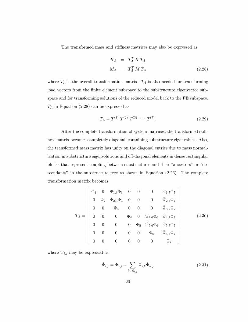
The transformed mass and stiffness matrices may also be expressed as

KA = T TA K TA

MA = T TA M TA (2.28)

where TA is the overall transformation matrix. TA is also needed for transforming

load vectors from the finite element subspace to the substructure eigenvector sub-

space and for transforming solutions of the reduced model back to the FE subspace.

TA in Equation (2.28) can be expressed as

TA = T (1) T (2) T (3) · · · T (7). (2.29)

After the complete transformation of system matrices, the transformed stiff-

ness matrix becomes completely diagonal, containing substructure eigenvalues. Also,

the transformed mass matrix has unity on the diagonal entries due to mass normal-

ization in substructure eigensolutions and off-diagonal elements in dense rectangular

blocks that represent coupling between substructures and their “ancestors” or “de-

scendants” in the substructure tree as shown in Equation (2.26). The complete

transformation matrix becomes

TA =

Φ1 0 Ψ1,3Φ3 0 0 0 Ψ1,7Φ7

0 Φ2 Ψ2,3Φ3 0 0 0 Ψ2,7Φ7

0 0 Φ3 0 0 0 Ψ3,7Φ7

0 0 0 Φ4 0 Ψ4,6Φ6 Ψ4,7Φ7

0 0 0 0 Φ5 Ψ5,6Φ6 Ψ5,7Φ7

0 0 0 0 0 Φ6 Ψ6,7Φ7

0 0 0 0 0 0 Φ7

(2.30)

where Ψi,j may be expressed as

Ψi,j = Ψi,j +∑

k∈Si,j

Ψi,kΨk,j (2.31)

20

where Si,j is the set of indices for ancestors of substructure i that are descendants of

substructure j. Note that this is a recursive relation, so each Ψk,j in Equation (2.31)

must be calculated before Ψi,j . Substituting this for individual entries in TA yields

the recursive relation

(TA)i,j =

Φj if i = j ,

Ψi,jΦj if i ∈ Rj ,

0 otherwise.

(2.32)

where Rj is the set of indices for descendants of substructure j.

Since we are interested in only a partial eigensolution for the global eigen-

problem for a FE model, the cutoff frequency ωA for substructures is selected based

on the frequency range of interest, so substructure eigenpairs with natural frequen-

cies above ωA are not included. As a result, the dimension of the substructure

eigenvector subspace is typically reduced by orders of magnitude compared to the

dimension of the original FE model. In the next chapter, we survey the eigensolu-

tion methods suitable for the reduced eigenvalue problem produced by the AMLS

transformation.

21

Chapter 3

Survey of Eigensolution

Methods

In Chapter 2, we defined the symmetric generalized eigenvalue problem in the sub-

structure eigenvector subspace in Equation (2.3). For the purpose of surveying

eigensolution methods, we can restate this eigenproblem for a single eigenpair as

follows.

KAφ = λMAφ (3.1)

where KA ∈ RnA×nA is diagonal and positive semi-definite, and MA ∈ R

nA×nA is

block-sparse and positive definite in general. As mentioned in Chapter 2, the mass

matrix in the FE discretization subspace, M , is positive semi-definite in general

because the mass matrix may be positive definite for a consistent mass formulation

or positive semi-definite for a lumped mass formulation. But, the AMLS transformed

mass matrix MA is positive definite because the zero mass degrees of freedom, which

are associated with infinite eigenvalues, are eliminated by substructure eigenspace

truncation in the AMLS transformation. For this eigenproblem, we are to find nE

22

mutually MA-orthogonal eigenvectors φi, (i = 1, 2, . . . , nE), such that

ΦTA KA ΦA = ΛA, ΦT

A MA ΦA = I, (3.2)

where ΛA ∈ RnE×nE = diag(λi), ΦA ∈ R

nA×nE = [φ1, φ2, · · · , φnE], and nA ≫ nE.

Note that the eigenvalues are ordered such that

λ1 ≤ λ2 ≤ · · · ≤ λnE. (3.3)

In the following sections, several eigensolution methods are discussed for our

reduced eigenproblem in Equation (3.1). Single vector iteration methods, subspace

iteration methods, Lanczos methods, and similarity transformation methods are

discussed in this chapter. The comparison between subspace iteration methods and

Lanczos methods for our reduced eigenproblem will be given in detail in Chapter 4,

so we discuss general concepts of both methods in this chapter instead of details

of applying the eigensolution methods to our reduced eigenproblem. Similarity

transformation methods are discussed because the new eigensolution algorithm in

Chapter 4 requires a robust and fast dense eigensolver. Note that we drop the

subscript A from the system matrices (KA and MA) and the matrices representing

the eigensolution for the reduced eigenproblem (ΛA and ΦA) for convenience and

brevity in the following sections.

3.1 Single Vector Iteration Methods

One of the oldest methods for solving eigenvalue problems is the power method.

Stodola used this method to compute the fundamental frequency of turbine shafts

of variable cross section in the early 1900s [44]. So this method is also called the

Stodola method.

The inverse iteration method is one example of the power/Stodola method.

The basic algorithm of inverse iteration is shown in Figure 3.1. Assuming K is

23

begin

initial guess x0

for k = 1, 2, ... do

1 xk = K−1Mxk−1

2 xk = xk/‖xk‖1M3 µk = xT

k Kxk

4 if converged then

λ = µk, φ = xk and stop

endend1‖x‖M = (xT Mx)1/2.

Figure 3.1: Basic algorithm for inverse iteration method

positive definite, a new iteration vector is generated by multiplying a previous iter-

ation vector by K−1M in step 1, and normalized with respect to the mass matrix

M in step 2 as shown in Figure 3.1. As the iteration number k increases, µk and

xk converge to the smallest eigenvalue λ and the corresponding eigenvector φ of

Equation (3.1).

For multiple eigenpairs, the deflation technique, or Gram-Schmidt orthogo-

nalization can be adopted [38, 41]. For Gram-Schmidt orthogonalization, one step

is added inside of the loop over k:

xk = xk −nc∑

i=1

(xTk Mφi)φi (3.4)

where nc is the number of previously converged eigenvectors. This step removes

the φi component in every iteration step by orthogonalizing an iteration vector xk

against φi with respect to M .

The convergence rate for the rth eigenvalue is |λr/λr+1|. This implies that

convergence strongly depends on the separation of the eigenvalues. The convergence

rate can be improved greatly by shifting [38, 45]. For this acceleration, step 1 can

be replaced in the iteration with:

xk = (K − σM)−1Mxk−1 = K−1σ Mxk−1 (3.5)

24

where σ is a shift corresponding to xk−1. Due to shifting, the convergence rate is

changed to |(λr − σ)/(λr+1 − σ)| and the eigenvalue becomes λ = µk + σ.

In practice, it is difficult to choose an appropriate shift in the iteration pro-

cess. One possibility is to use as a shift value the Rayleigh quotient [38, 39, 46]. This

method is called Rayleigh quotient iteration. If xk is reasonably close to the eigen-

vector of interest, then convergence of Rayleigh quotient iteration is cubic [38]. Even

though Rayleigh quotient iteration accelerates the convergence, it is more expensive

per iteration than plain inverse iteration, requiring a factorization of (K − σkM) at

every iteration if σk changes with each iteration. Inverse iteration is one of the most

widely used methods to compute an eigenvector for a tridiagonal matrix [63] because

factoring tridiagonal matrix is extremely inexpensive, but it is not appropriate for

solving very large generalized eigenproblems for multiple eigenpairs.

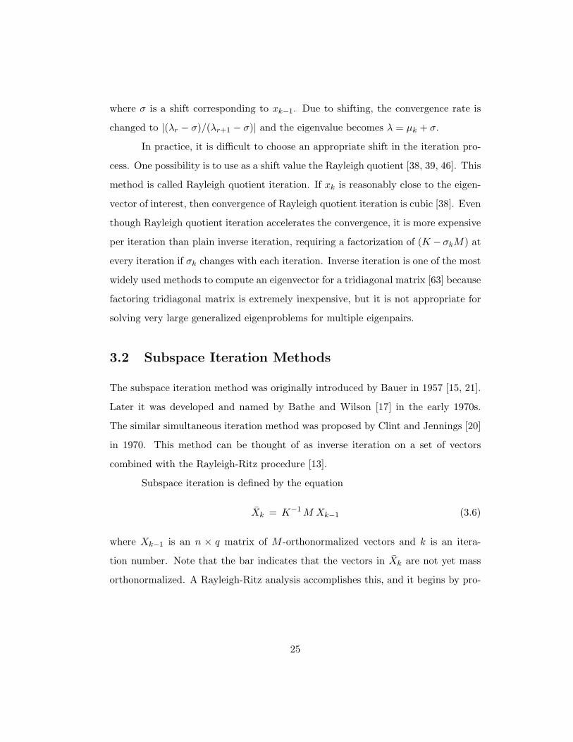
3.2 Subspace Iteration Methods

The subspace iteration method was originally introduced by Bauer in 1957 [15, 21].

Later it was developed and named by Bathe and Wilson [17] in the early 1970s.

The similar simultaneous iteration method was proposed by Clint and Jennings [20]

in 1970. This method can be thought of as inverse iteration on a set of vectors

combined with the Rayleigh-Ritz procedure [13].

Subspace iteration is defined by the equation

Xk = K−1 M Xk−1 (3.6)

where Xk−1 is an n × q matrix of M -orthonormalized vectors and k is an itera-

tion number. Note that the bar indicates that the vectors in Xk are not yet mass

orthonormalized. A Rayleigh-Ritz analysis accomplishes this, and it begins by pro-

25

jecting the stiffness and mass matrices onto the subspace created in the kth iteration:

Kk = XTk K Xk (3.7)

Mk = XTk M Xk (3.8)

where Kk and Mk are the projections of the system matrices onto the subspace

represented by the matrix Xk. The eigensolution can be obtained by solving the

following projected eigenvalue problem:

Kk Qk = Mk Qk Λk (3.9)

where Qk ∈ Rq×nc is a matrix containing eigenvectors, Λk ∈ R

nc×nc is a diago-

nal matrix containing eigenvalues, q is the number of iteration vectors, and nc is

the number of converged eigenpairs. Finally, new M -orthonormalized Ritz vectors

represented by Xk are generated by

Xk = Xk Qk (3.10)

The basic algorithm of the subspace iteration method is summarized in Figure 3.2.

The convergence rate of the ith eigenvalue when q iteration vectors are used is

|λi/λq+1|. To obtain a higher convergence rate, one can use more iteration vectors.

Bathe suggested that the number of iteration vectors for computing r eigenpairs

should be

q = min( r + 8, 2r ). (3.11)

The number of subspace iterations required depends on the q/r ratio. For

large q/r ratios, the number of subspace iterations required will be less whereas

the solution time required for each iteration will be large. On the other hand, for

small q/r ratios, a large number of subspace iterations may be required, although

the solution time for each iteration will be small. The optimal value of q for a given

problem is not known in advance.

26

begin

start with M -orthonormalized initial matrix, X0

for k = 1, 2, . . . do

Yk−1 = MXk−1

Xk = K−1Yk−1

Rayleigh-Ritz analysis

Kk = XTk Yk−1, Mk = XT

k MXk

solve the projected eigenproblem: KkQk = MkQkΛk

Xk = XkQk

end

if converged then exitend

Λ = Λk, Φ = Xk

end

Figure 3.2: Basic subspace iteration method for generalized eigenproblem

Due to the expense of the Rayleigh-Ritz procedure when many eigenpairs are

needed, the efficiency of subspace iteration is limited. To solve for a large number

of eigenpairs, some acceleration techniques have been developed [9, 13, 12, 14]. In

order to accelerate the iteration itself, several techniques, such as over-relaxation,

shifting, and the use of Chebyshev polynomials [9, 14, 15], have been used.

The number of iterations required for convergence also depends on how close

the starting subspace is to the eigenspace of interest. Frequently, a set of unit

vectors with unity at the degree of freedom with the smallest ratio (Ki,i/Mi,i) is

used [38]. Improved starting vectors obtained by dynamic condensation have also

been used for forming a better starting subspace [11, 10]. Several methods for finding

good starting vectors have been developed for subspace iteration in order to have the

iteration converge in fewer steps. Cheu et al. [11] investigated the effects of selecting

initial vectors on computational efficiency for a subspace iteration method. Kaplan

[1] showed that his accelerated subspace iteration method obtained least-dominant

eigenpairs within a couple of steps in substructure eigenvector subspace due to the

good quality of the starting subspace.

27

The subspace iteration method is one candidate for solving our reduced eigen-

problem, but it is very inefficient to apply our case because the Rayleigh-Ritz proce-

dure in the subspace iteration method is very expensive due to the large dimension

of a starting subspace for adequate accuracy.

3.3 Lanczos Methods

The Lanczos algorithm was first proposed in 1950 by C. Lanczos for reducing a

symmetric matrix to tridiagonal form. After Paige’s pioneering work in 1971 [40], the

Lanczos algorithm has been developed continuously as a powerful tool for extracting

some of the extreme eigenvalues of a real symmetric matrix. It is natural to see this

algorithm as the Rayleigh-Ritz procedure on a Krylov subspace [40]. Compared

with the subspace iteration method, it is relatively inexpensive to use to compute a

large number of eigenpairs of very large sparse matrices [16].

The Lanczos algorithm constructs an orthonormal basis for the Krylov sub-

space

Km = span { q1, (K−1M)q1, . . . , (K−1M)m−1q1 }

= span { q1, q2, . . . , qm } (3.12)

where q1 is an arbitrary starting vector, q j is a Lanczos vector orthonormal to

the previous j − 1 Lanczos vectors with respect to M , and m is the dimension

of the Krylov subspace. The Lanczos algorithm involves the transformation of a

generalized eigenproblem into a standard form with a tridiagonal matrix with smaller

dimension m, which is much less than the size of the eigenproblem. The tridiagonal

matrix and the orthogonal Lanczos vectors are computed by a three-term recurrence

relationship as follows [26]:

βjq j+1 = (K−1M)q j − αjq j − βj−1q j−1, j = 1, 2, . . . , m (3.13)

28

In the recurrence equation, αj and βj are defined as

αj = 〈K−1Mq j , q j〉M (3.14)

βj = ‖(K−1M)q j − αjq j − βj−1q j−1‖M (3.15)

where 〈·, ·〉M denotes an inner product with respect to M , such that 〈x ,y〉M =

xT My , and ‖ · ‖M is defined as ‖x‖M =

√

〈xT ,x 〉M . As a result, the tridiagonal

matrix becomes

Tm =

α1 β2 0

β2 α2 β3

β3. . .

. . .

. . .. . . βm

0 βm αm

(3.16)

The tridiagonalization process terminates at a value much smaller than n, which is

the dimension of the matrix, and eigenpairs are computed from solving the standard

tridiagonal eigenvalue problem

Tms =1

λs. (3.17)

The eigenvector corresponding to λk is computed by

φk = Qmsk, k = 1, 2, . . . , nc (3.18)

where Qm = [q1, q2, . . . , qm] and nc is the number of converged eigenvalues. The

basic Lanczos algorithm for a generalized symmetric eigenproblem is summarized in

Figure 3.3.

The tridiagonalization procedure, which is in step 1 to step 5 in the algorithm,

does not produce M -orthonormal vectors as desired in practice due to round-off er-

rors. This makes the Lanczos method less efficient especially for problems with

closely spaced eigenvalues. To remedy this problem, Gram-Schmidt orthogonaliza-

29

begin

set a starting vector q

q1 = q/‖q‖Mset β0 = 0Lanczos Loop:

for j = 1, 2, . . . , m do

1 pj = K−1(Mq j)

2 αj = pTj (Mq j)

3 r j = pj − αjq j − βj−1q j−1

4 βj = ‖r j‖M5 q j+1 = r j/βj

6 solve the eigenproblem Tms = θs as neededif converged then exit

end

compute the eigenpair approximations:φk = Qmsk, λk = 1/θk where k = 1, . . . , nc

end

Figure 3.3: Basic Lanczos algorithm for generalized symmetric eigenproblem

tion can be used, right after step 3 as follows.

r j = r j −j

∑

k=1

(rTj Mqk)qk −

nso∑

k=1

(rTj Mφk)φk, (3.19)

where nso is the number of selected Ritz vectors for selective orthogonalization.

There are several techniques to avoid loss of orthogonality in Lanczos vectors. The

second term on the right-hand side in Equation (3.19) represents a full reorthogo-

nalization against previous Lanczos vectors and the third term represents a selective

orthogonalization against selected converged Ritz vectors [23, 24, 38]. Also, a partial

reorthogonalization against previous Lanczos vectors when loss of orthogonality is

detected, was proposed by Simon [28].

A spectral transformation or shifting strategy is useful when many eigenso-

lutions are required and the eigenvalue distribution is clustered. By the spectral

transformation, the relative separation of eigenvalues is affected dramatically even

though their absolute separation is decreased [23]. This spread of the eigenvalues

30

Lanczos Loop:

for j = 1, 2, . . . do

1 Pj = (K − σM)−1(MQj)−Qj−1BTj

2 Aj = P Tj (MQj)

3 Rj+1 = Pj −QjAj

4 Compute the orthogonal factorization of Rj+1:Qj+1Bj+1 = Rj+1,where Bj+1 is upper triangular and QT

j+1(MQj+1) = I.5 Solve the eigenproblem Tjsk = skθk as needed,

where k = 1, 2, . . . , (blocksize× j)if converged then exit

end

Figure 3.4: Lanczos Loop for the block Lanczos algorithm

ensures fast convergence to the eigenvalues near σ. Step 1 can be modified with

shifted Kσ = (K − σM) such that

pj = (K − σM)−1Mq j , (3.20)

and λk = σ + 1/θk. The major cost for this fast convergence is the cost of a

symmetric factorization (K − σM) = LDLT , where L is an unit lower triangular

matrix and D is a diagonal matrix. Since the inertias of (K − σM) and D are

the same by Sylvester’s Inertia Theorem [40, 45], we can compute the number of

eigenvalues in the interval [σ1, σ2] within the spectrum by using two factorizations

of (K − σ1M) and (K − σ2M). Thus we can confirm the number of computed

eigenvalues by comparing the number of eigenvalues in the interval [σ1, σ2] from

the matrix inertias of (K − σ1M) and (K − σ2M), which provides robustness of

implementation. The strategy for choosing shifts should be carefully chosen so that

the total cost, including the cost of the factorizations and the costs of Lanczos

iterations, is minimized. Some heuristics are used for selecting an optimal sequence

of shifts in some implementations [23, 24].

The block strategy, in addition to the shifting strategy, is preferable for better

convergence when there are multiple eigenvalues and for better data management

31

on some computer architectures, particularly if (K − σM) factors are out of core.

As we notice in the basic Lanczos algorithm as shown in Figure 3.3 all the floating

point operations performed are matrix-vector or vector-vector operations, which are

very inefficient in terms of operation-to-memory-reference rate (or computational

intensity) for sparse matrices. To achieve high performance, those operations are

modified to matrix-matrix operations by the block strategy. One of the most robust

implementations of the block Lanczos algorithm was produced by Grimes, Lewis,

and Simon [23, 25] along with a sparse linear solver package. This is an implemen-

tation of a block Lanczos technique with a dynamic shift-invert scheme. The block

version of the Lanczos loop in the Lanczos algorithm is summarized in Figure 3.4. In

the figure, Qj is a block of Lanczos vectors, and Aj and Bj for the block tridiagonal

matrix Tj are analogous to the scalars αj and βj for the tridiagonal matrix Tm in

the basic Lanczos algorithm. In general, it is best to choose a blocksize as large as

the largest expected multiplicity of eigenvalues. A blocksize of 6 or 7 works well

on all systems [23], not only due to the multiplicity of eigenvalues but also due to

the I/O expense. In a system in which I/O is less costly, a blocksize of 3 is more

effective [24].

The factorizations typically represent the largest single cost in shift-invert

block Lanczos eigenanalysis. There is a large constant cost per a block Lanczos

iteration, comprising the matrix-block solve, matrix-block multiplication, QR fac-

torization of Rj+1 and reorthogonalizations as shown in Figure 3.4. Even though the

block version of Lanczos algorithm improves the computational intensity, the block

Lanczos algorithm has some significant performance bottlenecks for a huge size of

eigenproblem requiring many eigenpairs because of the limitation on blocksize and

the I/O cost relating to the Lanczos vectors for reorthogonalizations and the matrix

factors for matrix-block solve.

32

3.4 Similarity Transformation Methods

Two matrices A, B ∈ Rn×n are said to be similar if there exists a nonsingular

Q ∈ Rn×n such that

B = Q−1AQ. (3.21)

Equation (3.21) is called a similarity transformation. If Q is an orthogonal matrix,

i.e., QT Q = I [46], then by an orthogonal similarity transformation the standard

eigenproblem, Ax = λx , becomes

(QT AQ)y = λy , (3.22)

where y = QTx . It is evident that if (x , λ) is an eigenpair of A, then (QT

x , λ) is an

eigenpair of (QT AQ). With a suitable choice of an orthogonal matrix, the similarity

transformation technique can be used to reduce A to a simpler form.

Frequently Householder reflectors are used for solving dense eigenvalue prob-

lems, to construct an orthogonal matrix Q that tridiagonalizes the matrix A. To use

this approach on a generalized eigenvalue problem, it is common and convenient to

transform the eigenproblem to standard form first. Using Cholesky factorization of

the positive definite mass matrix M = UT U , we can transform a generalized eigen-

value problem, Kx = λMx , to standard form, Ay = λy , while maintaining the

symmetry of the original matrices, where A = U−T KU−1, U is upper triangular,

and x = U−1y .

After we have a symmetric standard eigenproblem, the most common method

to solve this eigenproblem has three phases [47, 68]: (1) reduction - reduce the given

symmetric matrix A to tridiagonal form T , (2) tridiagonal eigenproblem - compute all

or some of the eigenpairs of T , (3) backtransformation - transform T ’s eigenvectors

to A’s.

The initial reduction of A to tridiagonal form is made by a sequence of (n−2)

orthogonal Householder reflections. More detailed explanation of this algorithm can

33

be found in [45]. This algorithm is implemented in the LAPACK routine DSYTRD.

For the tridiagonal eigenproblem, Algorithm of Multiple Relatively Robust

Representation [66, 67] can be used to compute a full or partial eigensolution. Pre-

viously, there have been several algorithms to compute the eigensolution of the

tridiagonal problem, including tridiagonal QR iteration, the divide-and-conquer al-

gorithm, and bisection with inverse iteration. All of these require more than O(n2)

operations for a full eigensolution. However, Parlett and Dhillon [63, 66, 67] have

proposed a new O(n2) algorithm for computing all eigenvalues and eigenvectors for

a symmetric tridiagonal problem. This new algorithm was implemented in the LA-

PACK routine DSTEGR. This algorithm is faster than any other existing algorithms

and uses the least workspace.

For backtransformation, the eigenvectors can be obtained by simple matrix-

matrix multiplication QS, where S is a matrix whose columns are eigenvectors of T

and Q is a matrix representing the orthogonal matrix that was used for tridiagonal

reduction. However, since Q is usually not explicitly computed in the tridiagonal

reduction, we can form the product QS using Householder reflectors without forming

Q explicitly. An efficient block algorithm for this backtransformation is implemented

in the LAPACK routine DORMTR.

34

Chapter 4

A New Eigensolution Algorithm

In this chapter, characteristics of the reduced eigenproblem are carefully examined,

and two standard approaches for the reduced eigenproblem are discussed in terms

of computational efficiency. Then, a new eigensolution algorithm is introduced to

efficiently solve the reduced eigenproblem on the substructure eigenvector subspace.

After a brief preliminary overview of the new eigensolution algorithm is given, each

piece of the algorithm is explained in detail, using the same example problem used

for the AMLS transformation, in the later sections of this chapter. Finally, two

practical issues in computer implementation of this new algorithm are discussed,

along with proposed remedies for both problems.

4.1 Motivation for a New Eigensolution Algorithm

The primary objectives in designing a new eigensolution algorithm for the reduced

eigenvalue problem produced by AMLS are to compute a large partial eigensolution,

to minimize memory and disk space requirements by exploiting sparsity of matrices,

to minimize operation counts and maximize parallel efficiency for fast runtime, and

to be reliable. Note that we are looking for typically 10, 000 eigenpairs. In order

35

to develop a new eigensolution algorithm satisfying these requirements, it is neces-

sary to discuss the characteristics of the reduced eigenproblem generated by AMLS

first. We will then compare two possible candidate eigensolvers for our reduced

eigenproblem considering the characteristics of the problem.

4.1.1 Reduced Eigenproblem Characteristics

After projecting K and M onto the substructure eigenvector subspace using AMLS,

the transformed (or reduced) eigenproblem has the following characteristics:

1. The stiffness matrix is diagonal and its diagonal entries are substructure eigen-

values.

2. The mass matrix has unity on the diagonal entries and values less than unity

on off-diagonal entries. The fact that the values on off-diagonal entries are less

than unity can be simply proved by positive definiteness of the mass matrix

MA.

3. The approximate number of global eigenvalues within the frequency range of

interest can be estimated due to the facts above.

4. An off-diagonal block of the mass matrix is nonzero only if its rows and columns

correspond to an ancestor-descendant pair in the substructure tree as shown

in Equation (2.26). Nonzero off-diagonal blocks of the mass matrix are densely

populated.

5. According to Kaplan’s experience with his eigensolution method [1], a good

initial guess for a subspace containing the global eigenvectors can be obtained

easily and economically. This subspace is represented with a very sparse ma-

trix.

36

6. For practical frequency response analysis of structures, the accuracy of the

eigensolution is only required to be consistent with the accuracy available

from the FE discretization, rather than on the order of machine precision.

Only an approximate partial eigensolution is required.

7. The total number of substructure eigenvectors nA (≈ 105) kept using the

AMLS transformation is typically less than nF (≈ 107), the number of degrees

of freedom in the FE discretization, by orders of magnitude, but the reduced

eigenproblem is still too large to solve with conventional eigensolution algo-

rithms for dense problems.

8. The number of global eigenpairs required, nE, is typically about 104. For

frequency response applications, interest is primarily in the modal subspace

from which the frequency response is approximated rather than individual

eigenpairs.

Considering the characteristics above, we can consider a couple of existing

eigensolution methods for this large sparse problem. As mentioned in the preceding

chapter, candidates include the Lanczos method and the subspace iteration method.

In the next subsection, we will discuss the advantages and disadvantages of both

methods and arrive at a more promising approach for addressing our reduced eigen-

value problem.

4.1.2 Lanczos Method versus Subspace Iteration Method

The block Lanczos method is useful for large, sparse eigenproblems because the op-

erations involving the system matrices can take advantage of their sparsity. These

operations include symmetric indefinite factorization of (KA − σMA) with the nec-

essary values of the shift σ, linear equation solution for a block of vectors at each

iteration using the factored (KA − σMA) matrix, and matrix-matrix multiplication

37

Table 4.1: The number of natural frequencies in several frequency ranges for “8.4MDOF” model

Frequency rangeNumber of naturalfrequencies in range

1-100 Hz 581

100-200 Hz 990

200-300 Hz 1302

300-400 Hz 1520

400-500 Hz 1719

500-600 Hz 1852

with MA, as discussed in Chapter 3.

For a large eigenproblem with many modes needed, mass matrix multiplica-

tions require not only many floating point operations, but also a very large amount

of I/O when the sparse mass matrix is in secondary data storage. For example, if we

need 10,000 eigenpairs, 25, 000 or 30, 000 Lanczos vectors are typically required for

convergence, which require more than 2, 000 iterations with a rather large blocksize

of 12. Such a large number of mass matrix multiplications will be very expensive,

especially if MA is too large to fit in memory.

Because a large number of eigenpairs are sought, we frequently encounter

close spacing of eigenvalues, which causes slow convergence. As an example, Ta-

ble 4.1 presents the number of natural frequencies in several frequency ranges below

600 Hz for the “8.4M DOF” model, which will be used as a typical model with high

modal density in Chapter 6. As a frequency range becomes higher, the number

of natural frequencies within 100 Hz interval increases. Thus, the average number

of natural frequencies in 1 Hz interval within the frequency range between 500 Hz

and 600 Hz becomes about 18, which implies very close spacing of eigenvalues in

that frequency range. To accelerate the convergence, a shifting strategy is used.

If we expect typically around 200 converged eigenvalues per shift, dozens of shifts

and factorizations of the shifted stiffness matrix are required. In addition, although

38

KA is diagonal, the shifted stiffness matrix, (KA − σMA), is not diagonal so its

factorizations require many floating point operations.

If there are some clusters of eigenvalues within the spectrum of interest,

reorthogonalization must be done very carefully to avoid loss of orthogonality be-

tween Lanczos vectors. A lot of costly I/O is required for reading in preceding

Lanczos vectors of length 100, 000 for reorthogonalization as the iteration proceeds.

To overcome this defect, some techniques have been developed: full reorthogonaliza-

tion against previous Lanczos vectors, selective orthogonalization against converged

Ritz vectors, and partial reorthogonalization against Lanczos vectors when loss of

orthogonality is detected [23, 24, 27, 28]. However, the reorthogonalization is still

costly for Lanczos vectors of length 100,000.

As we have seen in the list of characteristics of our eigenproblem, a good

initial subspace for all of the desired global eigenvectors is available. The Lanczos

method, however, cannot exploit this initial guess for the entire subspace because

the Lanczos method operates with a small block of vectors and converges to only a

few eigenvectors at a time. It would be desirable to use an algorithm that can take

full advantage of the initial guess for the entire eigenvector subspace for the reduced

eigenproblem.

Subspace iteration is not as efficient as the Lanczos method in general [16],

but it may be better than the Lanczos method in our case, because a very good

starting subspace is represented with a very sparse matrix. Since we have a good

guess of the eigenspace1 for the reduced eigenproblem, convergence can be expected

in very few iteration steps. However, the dimension of the substructure eigenvector

subspace, typically 100, 000, is still too large for inexpensive Rayleigh-Ritz analysis.

The above considerations lead us to explore a new eigensolution algorithm

that takes the greatest possible advantage of subspace iteration, where the iteration

1In this dissertation, the term “eigenspace” is defined as a subspace spanned by eigenvectors ofthe matrix pencil (K, M), where K and M are stiffness and mass matrices, respectively.

39

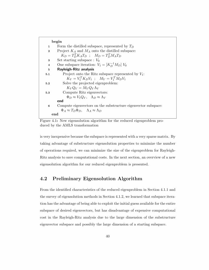
begin

1 Form the distilled subspace, represented by TD

2 Project KA and MA onto the distilled subspace:KD = T T

DKATD ; MD = T TDMATD

3 Set starting subspace : V0

4 One subspace iteration: V1 = [K−1D MD] V0

5 Rayleigh-Ritz analysis

5.1 Project onto the Ritz subspace represented by V1:KV = V T

1 KDV1 ; MV = V T1 MDV1

5.2 Solve the projected eigenproblem:KV QV = MV QV ΛV

5.3 Compute Ritz eigenvectors:ΦD ≈ V1QV , ΛD ≈ ΛV

end

6 Compute eigenvectors on the substructure eigenvector subspace:ΦA ≈ TDΦD, ΛA ≈ ΛD

end

Figure 4.1: New eigensolution algorithm for the reduced eigenproblem pro-duced by the AMLS transformation

is very inexpensive because the subspace is represented with a very sparse matrix. By

taking advantage of substructure eigensolution properties to minimize the number

of operations required, we can minimize the size of the eigenproblem for Rayleigh-

Ritz analysis to save computational costs. In the next section, an overview of a new

eigensolution algorithm for our reduced eigenproblem is presented.

4.2 Preliminary Eigensolution Algorithm

From the identified characteristics of the reduced eigenproblem in Section 4.1.1 and

the survey of eigensolution methods in Section 4.1.2, we learned that subspace itera-

tion has the advantage of being able to exploit the initial guess available for the entire

subspace of desired eigenvectors, but has disadvantage of expensive computational

cost in the Rayleigh-Ritz analysis due to the large dimension of the substructure

eigenvector subspace and possibly the large dimension of a starting subspace.

40

There is an opportunity for further reduction in order to improve the effi-

ciency of the subspace iteration method, if we can reduce the substructure eigenvec-

tor subspace without losing much accuracy. We can call this process “distillation”.

Within the “distilled” subspace, we can select a particularly good initial subspace

which is represented by a sparse matrix, and we can perform one subspace iteration

to refine it. Then we perform Rayleigh-Ritz analysis on the refined subspace to

approximate the global eigenpairs, and compute the eigenvectors on the substruc-

ture eigenvector subspace and on the FE discretization subspace subsequently. The

algorithm for this new eigensolution method is summarized in Figure 4.1.

For better understanding of this new algorithm in terms of subspaces used,

the relationships between subspaces in the new eigensolution method are illustrated

with their typical dimensions in Figure 4.2. We have the eigenproblem of 10 million

degrees of freedom (10M DOF) in the finite element subspace “F ”2. Using the

AMLS transformation, we can project the FE eigenproblem onto the AMLS subspace

(“A”) of dimension 100, 000 (100K). We distill the AMLS subspace and so obtain

new smaller distilled subspace (“D”) of typically dimension 40, 000 (40K). Then, we

form a truncated subspace “V0” of dimension 12, 000 (12K) in the distilled subspace

and do one subspace iteration to obtain the refined subspace “V1”. The approximate

global eigenspace “E” is computed by one Rayleigh-Ritz analysis on the refined

subspace V1. Finally, eigenvector computations on the subspace A and subsequently

on the subspace F can be done to obtain the approximate global eigensolution in

the original FE discretization subspace. Each of the steps of the new eigensolution

algorithm shown in Figure 4.1 is explored individually in the remainder of this

chapter.

2From now on, the subspaces used in the new eigensolution algorithm will be denoted withcalligraphic letters.

41

F

V0

A

D

V1E

F : FE subspace (10M) V0 : Truncated subspace of D (12K)A : AMLS subspace (100K) V1 : Refined subspace of D (12K)D : Distilled subspace of A (40K) E : Approximate global eigenspace (10K)

Figure 4.2: Subspaces of the new eigensolution method

4.3 Projection onto a Distilled Subspace

In the process of setting the parameters for the AMLS reduction from the FE sub-

space (F ) to the AMLS subspace (A), we investigated tradeoffs between substruc-

ture sizes, substructure eigenvalue cutoff values, global eigensolution accuracy and

computer resource usage. We observed that increasing the size of the “leaf” sub-

structure, which is a substructure does not have descendant in the substructure

tree, while keeping the same accuracy for the global eigensolution, decreases the

number of substructure eigenvectors kept, and allows the eigenvalue cutoff ωA

2 for

substructure eigenproblems to decrease. However, increasing the leaf substructure

size increases the time required for Phase3, the program executes the AMLS trans-

formation, because the cost of factoring substructure stiffness matrices and solving

substructure eigenvalue problems increases faster than the substructure size. More-

over, the memory usage of Phase3 increases significantly as the leaf substructure

42

size increases. This observation indicates that using larger leaf substructures for a

FE model results in a more compact substructure eigenvector subspace, but at the

cost of a substantial performance penalty in Phase3. This means that if the FE

model is divided into larger substructures, the substructure eigenvalue cutoff ωA

2

can be lowered while achieving the same global eigensolution accuracy as with a

smaller leaf substructure size.

Figure 4.3 summarizes the effects of varying the maximum size of leaf sub-

structures, on the number of substructure eigenvectors kept (or the dimension of

the subspace A) and the performance of Phase3 for a “Trim-Body” model, which

will be used for numerical results in Chapter 6. The target size of leaf substruc-

tures was varied from 700 to 12000. A consistent level of accuracy in the global

eigensolution was maintained by adjusting the substructure eigenvalue cutoff ωA

2 so

that the number of approximate global eigenpairs with natural frequencies below a

cutoff frequency of ωG = 2π · 600 Hz was equal to 4, 208 in all cases, according to

the inertias of the matrix (KA − ωG

2MA). Note that the inertia of the matrix A is

defined by the nonnegative number triple (ν(A), ζ(A), π(A)), each of which denotes

the number of negative, zero, and positive eigenvalues of A, respectively. From the

results in Figure 4.3, we can recognize that as the maximum leaf substructure size

increases, a smaller substructure eigenvector subspace (A), which gives the same ac-

curacy in the global eigensolution, can be obtained. The elapsed time and memory

usage, however, increase significantly as the maximum substructure size increases.

These results suggest that we can build a reduced subspace of the substruc-

ture eigenvector subspace without any performance penalty in Phase3. To do this,

we can compute and truncate the eigenpairs of a subtree, which is a node in the

substructure tree and all of its descendants down to the leaf level. In other words,

we can distill the substructure eigenvector subspace by combining together the sub-

structures that constitute a subtree of the substructure tree, and computing eigen-

43

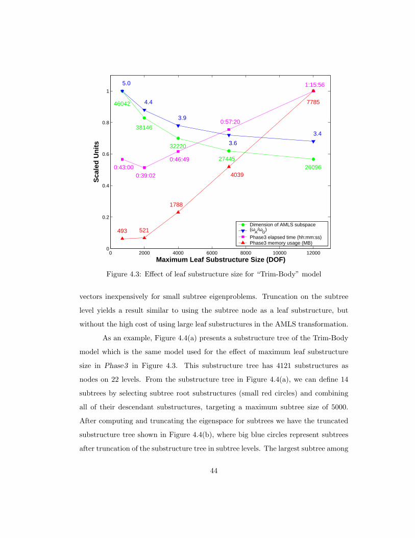
0 2000 4000 6000 8000 10000 120000

0.2

0.4

0.6

0.8

1

Maximum Leaf Substructure Size (DOF)

Sca

led

Un

its

5.0

4.4

3.9

3.6

3.4

46042

38146

32220

27445260960:43:00

0:39:02

0:46:49

0:57:20

1:15:56

493 521

1788

4039

7785

Dimension of AMLS subspace(ω

A/ω

G)

Phase3 elapsed time (hh:mm:ss) Phase3 memory usage (MB)

Figure 4.3: Effect of leaf substructure size for “Trim-Body” model

vectors inexpensively for small subtree eigenproblems. Truncation on the subtree

level yields a result similar to using the subtree node as a leaf substructure, but

without the high cost of using large leaf substructures in the AMLS transformation.

As an example, Figure 4.4(a) presents a substructure tree of the Trim-Body

model which is the same model used for the effect of maximum leaf substructure

size in Phase3 in Figure 4.3. This substructure tree has 4121 substructures as

nodes on 22 levels. From the substructure tree in Figure 4.4(a), we can define 14

subtrees by selecting subtree root substructures (small red circles) and combining

all of their descendant substructures, targeting a maximum subtree size of 5000.

After computing and truncating the eigenspace for subtrees we have the truncated

substructure tree shown in Figure 4.4(b), where big blue circles represent subtrees

after truncation of the substructure tree in subtree levels. The largest subtree among

44

(a) Substructure tree for Trim-Body model

(b) Truncated substructure tree for Trim-Body model

Figure 4.4: Substructure tree versus truncated substructure tree at subtree levelsfor Trim-Body model

45

3 6

Figure 4.5: Substructure tree truncation process. (a) Defining subtrees in the orig-inal substructure tree. (b) Truncated substructure tree after defining subtrees andtruncating subtree eigenspace.

the 14 subtrees in this model contains 509 substructures, and the total number of

FE degrees of freedom corresponding to this subtree is 218, 230. Therefore, defining

subtrees after the AMLS transformation has an effect of defining significantly larger

leaf substructures, and makes it possible to achieve the same accuracy with a lower

substructure eigenvalue cutoff.

For “branch substructures”, which are substructures that are not included

in subtrees represented with small red dots in Figure 4.4(b), we do not need to

solve an eigenproblem but merely truncate the substructure eigenspace using the

same cutoff frequency as for subtrees. With eigenspace truncation for both subtrees

and branch substructures, we can achieve reduction of the substructure eigenvector

subspace (A or the AMLS subspace), sacrificing little accuracy. Hence, the new

distilled subspace contains subtree eigenvectors for subtrees and Boolean vectors for

branch substructures. The distillation cutoff frequency ωD should be chosen based

on the accuracy we want to achieve.

46

To illustrate the distilling process, we use the same example model which was

used in the AMLS transformation in Section 2.2. For the plate model with seven

substructures as shown in Figure 2.1, we begin the distilling process of the substruc-

ture eigenvector subspace by identifying subtrees of the original substructure tree

shown in Figure 4.5(a). We select substructures 3 and 6 from Figure 4.5(a) as root

nodes for subtrees as the simplest possible examples. Each subtree has stiffness and

mass matrices that are simply the appropriate submatrices of KA and MA, with as

many rows and columns as the total number of substructure eigenvectors for the

subtree. Let us recall the AMLS transformed stiffness matrix KA in Equation (2.25)

and the AMLS transformed mass matrix MA in Equation (2.26). According to the

truncated substructure tree as shown in Figure 4.5(b), the stiffness matrix KA can

be partitioned as

KA =

Λ1 0 0

Λ2 0 0 0

Λ3

Λ4 0 0

Λ5 0 0

(sym.) Λ6

Λ7

(4.1)

=

(KA)s30 0

(KA)s60

(sym.) (KA)s7

(4.2)

47

Similarly, the mass matrix MA can be partitioned as

MA =

I1 0 (MA)1,3 (MA)1,7

I2 (MA)2,3 0 (MA)2,7

I3 (MA)3,7

I4 0 (MA)4,6 (MA)4,7

I5 (MA)5,6 (MA)5,7

(sym.) I6 (MA)6,7

I7

(4.3)

=

(MA)s30 (MA)s3,7

(MA)s6(MA)s6,7

(sym.) (MA)s7

(4.4)

where the subscript si,j denotes the coupling between the subtree i (or possibly

branch substructure i) and the branch substructure j, and the subscript si is an

abbreviation of the subscript si,i. Therefore, the stiffness matrix of the subtree

rooted at substructure 3 is simply a diagonal matrix of the form

(KA)s3=

Λ1 0 0

0 Λ2 0

0 0 Λ3

(4.5)

and the mass matrix of the subtree rooted at substructure 3 is:

(MA)s3=

I1 0 (MA)1,3

I2 (MA)2,3

(sym.) I3

(4.6)

where Ii represents an identity matrix corresponding to substructure i. The stiffness

and mass matrices for the subtree rooted at node 6 are similar. The eigenvalue

problem for each subtree is defined in terms of the subtree stiffness and mass matrices

as

(KA)si Φsi = (MA)si Φsi Λsi , i = 3, 6. (4.7)

48

In practice, the main consideration in the selection of a node as the root of

a subtree is the dimension of the resulting subtree eigenvalue problem. A target

dimension for the subtree eigenvalue problems will likely depend on how the cost

of the eigensolution increases with eigenvalue problem size. Suppose, for example,

that the cost of solving one of these problems increases as the cube of its dimension.

If root nodes for subtrees are too close to the root of the entire substructure tree,

the subtree eigenvalue problems can become too large and therefore excessively

expensive to solve. A partial eigensolution for subtrees is computed for eigenvalues

up to the distillation cutoff value ωD

2.

Solving the subtree eigenvalue problems and truncating their eigenspaces has

the effect of cutting off the branches of the substructure tree at the subtree root

nodes. The subtree effectively becomes a leaf substructure in the substructure tree,

and the tree becomes much simpler and smaller as a result of this truncation process

as illustrated in Figure 4.5.

In the example, node 7 is the only node in the substructure tree that has

not been included in subtrees 3 and 6, because it is “above” the subtree level.

For this branch substructure, truncating its eigenspace does not require an eigen-

value problem to be solved because the truncation is simply done by deciding which

substructure eigenvectors to keep, based on whether its eigenvalues are below the

distillation cutoff value ωD

2.

For the tree in Figure 4.5(b), the distilled subspace containing the subtree

eigenvectors and the Boolean vectors for the branch substructure is represented by

the matrix

TD =

Φs30 0

0 Φs60

0 0

I

0

s7

=

Φs30 0

0 Φs60

0 0 Bs7

(4.8)

49

Here the submatrices Φs3and Φs6

are rectangular and contain subtree eigenvectors.

The submatrix Bs7, containing identity and null matrices, has the effect of selecting

the substructure eigenvectors whose eigenvalues are below the cutoff value ωD

2, for

the branch substructure (node 7). The sparsity of this transformation matrix TD,

makes it inexpensive to project the matrices KA and MA onto its subspace.

By using this transformation matrix TD, the projection of the stiffness matrix

KA, shown in Equation (4.2), is given by

KD = T TD KA TD

= T TD

(KA)s30 0

(KA)s60

(sym.) (KA)s7

TD

=

Λs30 0

Λs60

(sym.) Λs7

(4.9)

assuming the orthonormality of subtree eigenvectors with respect to subtree mass

matrix. Similarly, the projection of the mass matrix MA in Equation (4.4) becomes

MD = T TD MA TD

= T TD

(MA)s30 (MA)s3,7

(MA)s6(MA)s6,7

(sym.) (MA)s7

TD

=

I 0 ΦTs3

(MA)s3,7Bs7

I ΦTs6

(MA)s6,7Bs7

(sym.) I

(4.10)

Eigenpairs of the problem KAΦA = MAΦAΛA can be approximated, using the

distilled subspace represented by the matrix TD, by projecting KA and MA onto

50

this subspace and solving the eigenvalue problem

KD ΦD = MD ΦD ΛD. (4.11)

The accuracy of this approximation will depend on the cutoff frequency ωD used

in truncation, where ωD is the cutoff frequency for subtree eigenproblems and for

branch substructure truncation. Note that instead of simply solving the eigenprob-

lem in Equation (4.11), we will approximate the solution of the eigenvalue problem

in Equation (4.11) using a truncated subspace, one subspace iteration, and one

Rayleigh-Ritz analysis as described in the following sections.

This projection onto the distilled subspace results in system matrices KD

and MD, which retain advantageous properties of KA and MA. The stiffness ma-

trix, KD, remains diagonal and its diagonal elements contain subtree eigenvalues,

and truncated sets of substructure eigenvalues for branch substructures. The mass

matrix, MD, also keeps the sparsity pattern according to the truncated substructure

tree shown in Figure 4.5(b), but nonzero off-diagonal elements in MA within a sub-

tree are eliminated by solving the subtree eigenvalue problem. Therefore, the mass

matrix MD has fewer nonzero elements than the mass matrix MA. Furthermore,

the computational cost of multiplying V1 by MD in Rayleigh-Ritz analysis would

be inexpensive due to the reduced number of nonzero elements of the mass matrix

MD. The cost of projecting the reduced eigenproblem onto the distilled subspace

depends mostly on the cost of solving subtree eigenvalue problems, which strongly

depends on the target dimension of these eigenvalue problems. The effect of the

target size of subtrees on the eigensolution accuracy and the timing performance is

investigated for two models in Chapter 6.

There are many reasons for projecting the eigenvalue problem onto the dis-

tilled subspace. First, the main cost is that of solving perhaps a few dozen small

subtree eigenproblems, which are inexpensive to solve because of their size and can

be solved in parallel. Because the distilled subspace is represented by the block

51

diagonal rectangular matrix, TD, the projection onto this subspace is inexpensive.

The stiffness matrix KA becomes the smaller diagonal matrix KD. For the mass

matrix MA, the projection is done by simply premultiplying off-diagonal submatri-

ces corresponding to ancestor of a subtree in MA by the subtree eigenvectors and

truncating the columns according to the Boolean matrices for branch substructures

as shown in Equation (4.10). Since we just truncate the substructure eigenpairs for

branch substructures, we do not need to compute any branch substructure eigen-

pairs whose eigenvalues are above the distillation cutoff value ωD

2 in the initial

AMLS transformation. This fact reduces the cost of the AMLS transformation for

branch substructures. Since the system matrices KD and MD are reduced and sim-

plified in subtree levels, we can more reliably identify good vectors for a starting

subspace in subtree levels. As a result, we can have a smaller starting subspace for

the final Rayleigh-Ritz eigenproblem on the distilled subspace.

4.4 Starting Subspace

The choice of the starting subspace plays a critical role in our eigensolution analysis

because the dimension of the starting subspace determines the cost of the entire

eigensolution process. Hence, we want to minimize the starting subspace dimen-

sion while achieving acceptable accuracy with one subspace iteration. A starting

subspace should be very close to the eigenspace of the distilled eigenproblem of

Equation (4.11).

In the distilled subspace, we have the diagonal matrix KD and the block-

sparse matrix MD that has values of unity on the diagonal elements and values

less than unity on the off-diagonal elements. In a crude approximation, the mass

matrix MD resembles an identity matrix. If the system matrices KD and MD are

diagonal, the unit vectors with the values of unity corresponding to those degrees

of freedom that have the smallest ratios (KD)ii/(MD)ii, are the eigenvectors corre-

52

sponding to the smallest eigenvalues. Since we have the system matrices KD and

MD which are diagonal and close to a diagonal form, respectively, we can expect

a good starting subspace by collecting unit vectors corresponding to the smallest

ratios (KD)ii/(MD)ii. Therefore, a good starting subspace can be constructed by

collecting unit vectors that have ones in the rows corresponding to the eigenvalues

less than some cutoff value for subtrees and branch substructures.

To construct a starting subspace, we might need two different cutoff frequen-

cies. One is ωst

Vfor subtrees and the other is ωbs

Vfor branch substructures. Since we

improve the eigenproperties in the subtree levels by computing subtree eigensolution,

the subtree cutoff frequency, ωst

V, for selecting initial vectors being included in the

starting subspace might be very close to the global cutoff frequency ωG. For branch

substructures, however, a cutoff frequency ωbs

Vmight be larger than the subtree cut-

off frequency ωst

Vfor accuracy because we do just truncate the branch substructure

eigenspace in the distillation process. The effects of the two cutoff frequencies for

subtrees and branch substructures in forming a starting subspace are investigated

later for two models in Chapter 6.

After we select the cutoff frequencies for a starting subspace, the initial vec-

tors are collected based on the cutoff values for subtrees and branch substructures

to form a matrix. The dimension of the starting subspace is the dense eigenproblem

dimension in Rayleigh-Ritz analysis. Since the cost of solving the Rayleigh-Ritz

eigenproblem increases as the cube of its dimension, the cutoff frequencies for the

starting subspace must be determined to achieve the minimum dimension of starting

space with acceptable accuracy and affordable computational costs. If a more accu-

rate eigensolution is required, the size of the starting subspace should be increased

by choosing higher cutoff values for the subtrees and branch substructures, but this

will result in more computational costs.

As a result of selecting unit vectors for subtrees and branch substructures,

53

the matrix representing the starting subspace for solving the eigenvalue problem

shown in Equation (4.11) can be expressed as

V0 =

I

0

s3

0 0

0

I

0

s6

0

0 0

I

0

s7

(4.12)

The null submatrix in the rectangular matrix, [ I 0 ]Tsi, indicates that the eigen-

values for subtrees 3 and 6 are truncated based on the cutoff value for subtrees ωst

V.

Similarly, the eigenvalues for the substructure 7 are truncated based on the other

cutoff value for branch substructures ωbs

V. Due to the block identity submatrices in

the matrix V0 and the fact that the matrices KD and MD are diagonal and block-

sparse, respectively, the new subspace improved by one “inverse iteration”, is still

represented by a sparse matrix, as will be shown in the next section.

54

4.5 Subspace Improved by One “Inverse Iteration”

The improved (or refined) subspace can be obtained by using one “inverse iteration”

(or subspace iteration) of the form

V1 = K−1D (MD V0)

= K−1D

I

0

0 ⊛

0

I

0

⊛

⊛ ⊛

I

0

(4.13)

where a “⊛” represents a nonzero block in the product (MDV0).

Multiplying V0 by MD produces a matrix that is just a collection of the

columns of MD corresponding to nonzero rows of the matrix V0. Also, premulti-

plying this matrix by K−1D simply scales the rows of the product (MDV0) with the

eigenvalues of subtrees and branch substructures. We simply delete some columns

of MD based on the sparsity of V0 to form (MDV0), so that there is no floating point

operation at all in this sparse iteration process. The only cost in this sparse iteration

is the cost of scaling with diagonal K−1D , resulting in a number of multiplications

equal to the number of nonzero off-diagonal elements in (MDV0). So computing

the matrix V1 representing the refined subspace is very economical and the matrix

V1 is still sparse due to the identity submatrices in the matrix V0 representing the

starting subspace. The sparse matrix V1 shown in Equation (4.13) requires much

less memory and disk space, if we store only nonzero submatrices, than a full matrix

would.

One more refinement by inverse iteration, possibly using a shifting strategy,

would improve the accuracy of the eigensolution, but it would cost much more since

55

the matrix representing the new subspace would be fully populated. Therefore, our

goal is to choose ωV just high enough to achieve acceptable accuracy with only one

iteration.

4.6 Rayleigh-Ritz Analysis

Rayleigh-Ritz analysis for a given Ritz subspace involves three phases: (1) projec-

tion onto Ritz subspace − project the given system matrices onto the given Ritz

subspace, (2) eigenproblem for Ritz values − compute the required eigenpairs of the

projected problem, (3) computation of Ritz eigenvectors − convert eigenvectors of

the projected problem to eigenvectors of the larger original problem. Each phase is

explained in detail for our problem below.

To extract an approximate eigensolution, the eigenvalue problem must be

solved on the refined subspace (V1) represented by the matrix V1. The stiffness and

mass matrices are projected onto the subspace represented by the matrix V1 as

KV = V T1 KD V1 and MV = V T

1 MD V1. (4.14)

This leads to the following projected eigenvalue problem

KV QV = MV QV ΛV , (4.15)

where ΛV is a diagonal matrix containing eigenvalues and the columns of QV are

the MV -orthonormalized eigenvectors.

The generalized eigenvalue problem in Equation (4.15) can be reduced to a

standard symmetric eigenvalue problem, using a Cholesky factorization of the mass

matrix, MV = UT U , as

AV XV = XV ΛV (4.16)

where

AV = U−T KV U−1, XV = UQV (4.17)

56

and U is an upper triangular matrix. Due to the dimensional reduction to the

distilled subspace and then to the starting subspace, the dimension of this final

eigenproblem is not much larger than the number of eigenpairs required. Hence,

this is a dense eigenvalue problem requiring almost the full eigensolution that can

appropriately use Householder reduction to tridiagonalize the matrix AV .

After tridiagonalization of the matrix AV , we have the eigenproblem TS =

SΛ, where T = QT AV Q and Q is the orthogonal matrix which was used to tridi-

agonalize the matrix AV . For this tridiagonal eigenproblem, we can use the new

algorithm by Dhillon [63] which requires only O(nV

2) operations for a partial or full

eigensolution, where nV is the dimension of the eigenproblem. The algorithm is re-

ferred to as Algorithm MRRR (multiple relatively robust representations) [66, 67, 68].

Using the bidiagonal factorization T = LDLT as an RRR, desired eigenvalues are

computed to high relative accuracy and partitioned into clusters according to their

relative gaps [63, 67, 68]. Here, L is an unit lower triangular matrix and D is a di-

agonal matrix. For clusters with one eigenvalue, i.e., well separated eigenvalues, the

corresponding eigenvectors are computed by inverse iterations and twisted factor-

ization without any orthogonalization process based on the fact that the computed

eigenvectors are numerically orthogonal when the eigenvalues have large gaps. For

clusters with multiple eigenvalues, i.e., the eigenvalues have small relative gaps, Al-

gorithm MRRR uses multiple factorizations (LcDcLTc = LDLT − τcI) by choosing

the shifts τc to make relative gaps between clustered eigenvalues bigger. This pro-

cess is recursively performed until the relative gaps between clustered eigenvalues

are big enough to ensure orthogonality between eigenvectors.

The eigenvectors of the tridiagonal matrix are backtransformed by using

Householder reflectors which were generated in the tridiagonal reduction stage.

Therefore, we can solve the final standard eigenvalue problem in Equation (4.16)

using the most efficient and reliable dense eigensolver.

57

Rayleigh-Ritz analysis

• KV = V T1 KDV1, ←− projection onto Ritz subspace

MV = V T1 MDV1

• KV QV = MV QV ΛV ←− eigenproblem for Ritz values1 Factor MV = UT U2 Form AV = U−T KV U−1 for AV XV = XV ΛV

3 Householder Eigensolution

◦ QT AV Q = T ← reduce to tridiagonal matrix◦ TS = SΛ ← solve tridiagonal eigenproblem◦ XV = QS ← backtransform eigenvectors

end

4 Solve UQV = XV for QV to backtransform eigenvectors• ΦD ≈ V1QV ←− computation of Ritz eigenvectors

ΛD ≈ ΛV ≈ Λend

Figure 4.6: Algorithm for Rayleigh-Ritz analysis on the Ritz subspace V1

After we have computed the eigenpairs of the standard eigenvalue problem,

the eigenvectors corresponding to those of the generalized eigenproblem of Equa-

tion (4.15) are computed. This requires UQV = XV to be solved for QV .

The Ritz eigenvectors in the subspace D are finally approximated as follows:

ΦD ≈ V1 QV (4.18)

This matrix-matrix multiplication can be done on the level of individual subtrees

and branch substructures, if the sparse column block of V1 corresponding to each

subtree or branch substructure is stored appropriately. This multiplication can be

done economically due to the sparsity of V1 and is easy to parallelize because the

matrix V1 has already been divided into column blocks corresponding to subtrees

and branch substructures, and the matrix QV is available for all the processors. The

algorithm for the Rayleigh-Ritz analysis is summarized in Figure 4.6.

58

4.7 Computation of Eigenvectors on the Subspace A

Once we obtain the eigensolution in the distilled subspace, we need to recover the

eigenvectors ΦA as

ΦA ≈ TD ΦD (4.19)

and the eigenvalues as ΛA ≈ ΛD. As shown in Equation (4.8), TD is a block

diagonal matrix with Φsi or Bsi on its diagonal block. Due to this sparsity of

TD, the computation in Equation (4.19) is inexpensive and easily parallelizable.

More detailed algorithm for this computation is shown when the parallelism of this

algorithm is explained in Chapter 5.

4.8 Practical Issues in Numerical Implementation

When we factor the projected mass matrix MV (step 1 in Figure 4.6) we have

observed that the factorization sometimes fails because the matrix MV is not positive

definite. There are two reasons for factorization failure in the projected mass matrix

MV :

• linearly dependent vectors (or nearly linearly dependent vectors) in the refined

subspace represented by the matrix V1.

• indefiniteness of the mass matrix resulting from poor finite element modelling

practice.

These practical issues must be properly handled so that we are guaranteed to have

a good approximation of the eigensolution. We explain why these problems occur

and show remedies of the problems.

59

4.8.1 Low Frequency Modes

Rigid body modes and low frequency modes cause the stiffness matrix to be singular

or ill-conditioned. This singular or ill-conditioned stiffness matrix KD can cause

problems in forming a refined subspace represented by V1 by inverse iteration. Since

the entries in the diagonal stiffness matrix KD corresponding to rigid body modes

are zeros, the inverse of KD does not exist. Singularity of KD can be addressed by

deflating the system matrices [1]. Since the eigenvectors for the substructure at the

root of the tree corresponding to zero eigenvalues represent the global rigid body

modes [1], we can easily separate the rigid body modes from the flexible modes of

the system to avoid singularity of KD.

Columns of V1 might become nearly linearly dependent due to very small

substructure eigenvalues. The near linear dependence of columns of V1 comes from

premultiplying by the inverse of the nearly singular stiffness matrix KD. For exam-

ple, if (λ1)s7(the first eigenvalue in substructure 7 in the tree of Figure 4.5) is very

small, all the column vectors in V1 have a nonzero in (λ1)s7’s row because of mul-

tiplication of V0 by MD, and this nonzero becomes very large after multiplication

by the diagonal matrix K−1D as shown in Equation (4.13). Therefore, all columns

of V1 become near multiples of (e1)s7, which is the Euclidean unit vector with one

in (λ1)s7’s row in substructure 7. Because of this near linear dependence in V1,

Cholesky factorization can fail for the projected mass matrix which is formed by the

matrix triple product MV = V T1 MD V1.

We can eliminate near linear dependence in V1, by zeroing the row corre-

sponding to unity in (e1)s7, except in the column corresponding to (λ1)s7

, and

60

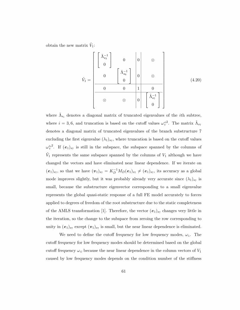
obtain the new matrix V1:

V1 =

Λ−1s3

0

0 0 ⊗

0

Λ−1s6

0

0 ⊗

0 0 1 0

⊗ ⊗ 0

Λ−1s7

0

(4.20)

where Λsi denotes a diagonal matrix of truncated eigenvalues of the ith subtree,

where i = 3, 6, and truncation is based on the cutoff values ωst

V

2. The matrix Λs7

denotes a diagonal matrix of truncated eigenvalues of the branch substructure 7

excluding the first eigenvalue (λ1)s7, where truncation is based on the cutoff values

ωbs

V

2. If (e1)s7is still in the subspace, the subspace spanned by the columns of

V1 represents the same subspace spanned by the columns of V1 although we have

changed the vectors and have eliminated near linear dependence. If we iterate on

(e1)s7, so that we have (v1)s7

= K−1D MD(e1)s7

6= (e1)s7, its accuracy as a global

mode improves slightly, but it was probably already very accurate since (λ1)s7is

small, because the substructure eigenvector corresponding to a small eigenvalue

represents the global quasi-static response of a full FE model accurately to forces

applied to degrees of freedom of the root substructure due to the static completeness

of the AMLS transformation [1]. Therefore, the vector (e1)s7changes very little in

the iteration, so the change to the subspace from zeroing the row corresponding to

unity in (e1)s7except (v1)s7

is small, but the near linear dependence is eliminated.

We need to define the cutoff frequency for low frequency modes, ωL. The

cutoff frequency for low frequency modes should be determined based on the global

cutoff frequency ωG because the near linear dependence in the column vectors of V1

caused by low frequency modes depends on the condition number of the stiffness

61

matrix KD. The condition number of KD is determined by the ratio of the largest

eigenvalue to the smallest eigenvalue in the diagonal elements of KD. Therefore, the

ratio ωG/ωL should be maintained for the large value of ωG to avoid the near linear

dependence in the column vectors of V1. By applying this technique we can avoid

factorization failures for the mass matrix MV resulting from near linear dependence

in V1. In the next subsection, we will discuss a remedy for non-positive definite mass

matrices MV caused by indefiniteness of FE mass matrices.

4.8.2 Indefinite Mass Matrix

Occasionally, we encounter an indefinite mass matrix in some FE models. From the

physical point of view, the mass matrix should be positive definite, as discussed in

Chapter 3. An indefinite mass matrix, MV , results from poor FE modelling practice.

Nearly zero or negative eigenvalues of MV result from, as an example, FE model

updating using experimental modal test data in some FE degrees of freedom to get

good correlation between FE model and experimental model. We should be able to

handle this problem in numerical computation for robustness of implementation.

When we have an indefinite mass matrix MV in Rayleigh-Ritz analysis, the

Cholesky factorization for transforming generalized eigenproblem to a standard form

would fail for this matrix so that we cannot solve the eigenvalue problem. To over-

come this difficulty in the projected mass matrix MV , we need to construct positive

definite matrix by using a shifting strategy. We can find the shifting parameter ρ

such that the shifted mass matrix (MV + ρKV ) is positive definite since the linear

combination of KV and MV should be positive definite in engineering practice.

By shifting, the eigenvalue problem becomes

KV p = µ (MV + ρ KV ) p. (4.21)

If we rearrange the equation above, we can recover the original eigenvalue problem

62

of the form

KV qV

= λV MV qV

(4.22)

where

λV =µ

1− ρµ, q

V=

1√1− ρµ

p (4.23)

and scaling the vector p by 1√1−ρµ

is for mass-normalization. The shift ρ can be

determined large enough to avoid indefiniteness of the mass matrix, but it should

be small enough that the eigenproperties of MV is not much affected. For example,

if we set ρ = 1/ωG

2 = 1/λG and we are looking for the eigenvalues between zero and

λG (= ωG

2), then the range of µ becomes

0 ≤ µ ≤ µG =λG

1 + ρλG

=λG

2. (4.24)

Therefore, the effect of shifting is to reduce the radius of the original spectrum by

half. After solving the eigenvalue problem of Equation (4.21), we can backtransform

the eigenpairs to the unshifted eigenpairs using the relations between the eigenpairs

in Equation (4.23).

63

Chapter 5

Parallel Implementation of the

New Algorithm

In this chapter, we focus on parallelization of the new eigensolution algorithm on

shared memory multiprocessors (SMM). As a popular example of SMM, there are

server workstations manufactured by many computer companies which have typi-

cally 2 to 8 processors with a large amount of shared memory. The machine used

for numerical results and performance in Chapter 6 is a server workstation that

has 4 processors with 8 gigabytes of shared memory. These types of machines are

used heavily in industry for AMLS because they are so cost-effective, and because

AMLS made it possible to use these machines instead of Cray supercomputers for

large-scale vibration analysis [1, 6]. The parallelization on distributed memory mul-

tiprocessors (DMM) will be discussed in Chapter 7 as future work for improving the

computer implementation of the new eigensolution algorithm.

As a tool for parallel implementation on SMM, the OpenMP Application

Program Interface (API) is used for the new eigensolution algorithm. OpenMP

consists of a set of compiler directives that manage the parallelism in the source

code, along with supporting runtime library routines and environment variables [50].

64

For 2 to 8 processor shared memory machines, OpenMP provides good scalability

with affordable effort and minimal changes in the source code. OpenMP requires a

special compiler and a runtime library that supports OpenMP. Due to the popularity

of SMM, every major computer vendor has provided a compiler and runtime library

for OpenMP.

There are many opportunities for parallelizing the new eigensolution algo-

rithm due to the nature of substructuring. In other words, the data that we handle

are naturally partitioned into blocks corresponding to subtrees and branch sub-

structures, so that the computation in each step of the eigensolution algorithm in

Figure 4.1 can be performed for subtrees and branch substructures. To achieve

high performance on a SMM, major considerations for parallelism are to reduce

the communication cost compared to the computational cost and to localize the

computational data as much as possible. Multiple processors communicate with

each other through ordinary reads and writes to shared variables in the program

with the OpenMP API for SMM machines. It is necessary to coordinate the ac-

cess to the shared variables across multiple processors. Because multiple processor

simultaneous accesses to the same shared variables can potentially cause incorrect

values, explicit coordination between processors, which is called “synchronization”,

is needed. By avoiding synchronization and localizing the data for computation as

much as possible we can reduce the communication cost. Therefore, we need an

algorithm that lets each processor perform as much computation as possible on its

own local data. The new eigensolution algorithm satisfies this requirement to a great

extent, because the computation for different subtrees and branch substructures can

be performed independently and simultaneously.

Before a sequential code is parallelized, it should be optimized as a sequential

code first. The sequential code of the new eigensolution algorithm was initially

optimized to a great extent for good sequential performance. In practice, by profiling

65

Table 5.1: Sequential performance of the new algorithm implementation for “Full-Vehicle” model.

step elapsed time(sec.) percent(%)

(a) Getting basic data 18 0.47(b) Projecting onto subspace D 889 23.41(c) One subspace iteration to form V1 6 0.16(d) Rayleigh-Ritz analysis on V1 2337 61.53(e) Computing approximate eigenvectors on A 498 13.11(f) Writing out eigensolution 50 1.32

total 3798 100.00

which operations take the most time in optimized sequential implementation, we can

determine which parts of the new algorithm should be parallelized to speed up the

overall timing performance. Table 5.1 shows the overall timing profile for all the

steps in sequential mode. A “Full-Vehicle” model, which will be discussed in detail

in Chapter 6, was used for this performance data.

The Rayleigh-Ritz analysis accounts for most of the elapsed time as shown in

Table 5.1. So we have to look at the algorithm of the Rayleigh-Ritz analysis in more

detail for parallelization. Projecting the reduced eigenproblem onto the distilled

subspace (D) and computing approximate eigenvectors on the AMLS subspace (A)

also have significant percentages in the timing profile. Therefore, we investigate

parallel algorithms for those steps in more detail in the following sections.

5.1 Parallelism for Projection onto the Distilled Sub-

space

Solving subtree eigenproblems to form the distilled subspace D and projecting sys-

tem matrices onto the distilled subspace are the significant parts of the computation

in steps 1 and 2 of the new algorithm in Figure 4.1. Almost 24% of the total elapsed

time is spent in this step as shown in Table 5.1. By considering the algorithm more

66

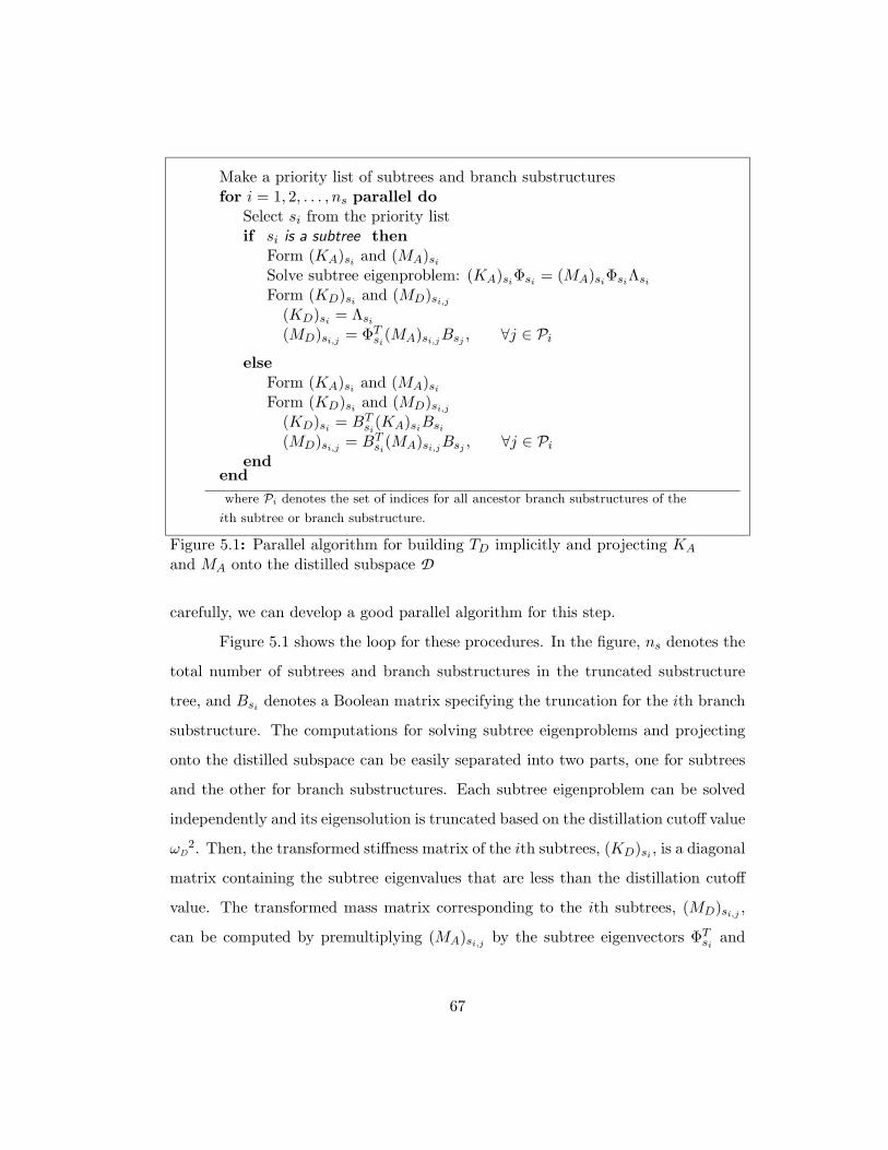
Make a priority list of subtrees and branch substructuresfor i = 1, 2, . . . , ns parallel do

Select si from the priority listif si is a subtree then

Form (KA)si and (MA)si

Solve subtree eigenproblem: (KA)siΦsi = (MA)siΦsiΛsi

Form (KD)si and (MD)si,j

(KD)si = Λsi

(MD)si,j = ΦTsi

(MA)si,jBsj , ∀j ∈ Pi

else

Form (KA)si and (MA)si

Form (KD)si and (MD)si,j

(KD)si = BTsi

(KA)siBsi

(MD)si,j = BTsi

(MA)si,jBsj , ∀j ∈ Pi

endend

where Pi denotes the set of indices for all ancestor branch substructures of the

ith subtree or branch substructure.

Figure 5.1: Parallel algorithm for building TD implicitly and projecting KA

and MA onto the distilled subspace D

carefully, we can develop a good parallel algorithm for this step.

Figure 5.1 shows the loop for these procedures. In the figure, ns denotes the

total number of subtrees and branch substructures in the truncated substructure

tree, and Bsi denotes a Boolean matrix specifying the truncation for the ith branch

substructure. The computations for solving subtree eigenproblems and projecting

onto the distilled subspace can be easily separated into two parts, one for subtrees

and the other for branch substructures. Each subtree eigenproblem can be solved

independently and its eigensolution is truncated based on the distillation cutoff value

ωD

2. Then, the transformed stiffness matrix of the ith subtrees, (KD)si , is a diagonal

matrix containing the subtree eigenvalues that are less than the distillation cutoff

value. The transformed mass matrix corresponding to the ith subtrees, (MD)si,j ,

can be computed by premultiplying (MA)si,j by the subtree eigenvectors ΦTsi

and

67

postmultiplying ΦTsi

(MA)si,j by the Boolean submatrix Bsj corresponding to the jth

branch substructure, which is the ancestor of the ith subtree. Since Bsj is a Boolean

matrix corresponding to the jth branch substructures, we can form this last product

by simply deleting the columns of ΦTsi

(MA)si,j corresponding to null rows in Bsj .

For branch substructures, the transformation matrices are Boolean matrices, which

represent truncation effects. So the projection is done by simply deleting the rows

and columns corresponding to the eigenvalues that are larger than the distillation

cutoff value ωD

2.

For efficient parallel performance, the parallelism for projection onto the dis-

tilled subspace D can be applied to the outermost loop in the algorithm shown in

Figure 5.1. For multiple processors, the work inside the outermost loop is parti-

tioned into units of the work according to subtrees and branch substructures. The

units of the work, partitioned according to subtrees and branch substructures, are

distributed to all the processors in order, and then each processor executes the as-

signed units of the work. This partitioning of the work in the loop over the subtrees

and branch substructures among the processors is called work-sharing [50]. The

heaviest part of the work inside the outermost loop is computing subtree eigen-

problems. The dimensions of the subtree eigenproblems are not the same because

the subtree eigenproblems are determined by how subtrees are defined in the given

substructure tree. In other words, different subtrees contain different number of sub-

structures having different number of substructure eigenpairs. This fact introduces

the load imbalance issue in parallelization of this algorithm.

In order to overcome this load imbalance problem, we need to use dynamic

scheduling [50, 51] for subtrees and branch substructures. In dynamic scheduling,

the assignment of subtree eigenproblems to processors is made at runtime. Not

all subtree eigenproblems are assigned to processors at the start of the loop. In-

stead, each processor requests another subtree eigenproblem after it has completed

68

P0

subtree 1

subtree 3

P1 subtree 2

idle time

start of parallel region synchronization point

elapsed time

(a)

P0

P1

subtree 1 subtree 3

subtree 2

idle time

start of parallel region synchronization point

elapsed time

(b)

Figure 5.2: Dynamic scheduling and efficient ordering examples for parallelizationof subtree eigenproblems. (a) Efficient ordering with dynamic scheduling. (b) Inef-ficient ordering with dynamic scheduling.

the work already assigned to it. For example, suppose we have 2 processors and

3 subtree eigenproblems as shown in Figure 5.2(a), where the length of a subtree

red box represents the elapsed time for a subtree eigenproblem. At the beginning,

two subtree eigenproblems are assigned to two processors, respectively. Then the

last eigenproblem for subtree 1 is assigned to processor 1, which finishes to solve

the assigned subtree 2 eigenproblem first, instead of waiting for processor 0 to fin-

ish. Figure 5.2(a) shows that dynamic scheduling helps to reduce the idle time of

processors in parallel region.

For optimal performance, we need to efficiently distribute the subtree eigen-

69

problems of different size to the processors by reordering the subtree eigenproblems

according to their dimension, so that the largest subtree eigenproblem is solved first

[54]. If the subtree eigenproblems are distributed in a different way, however, the

parallel performance is degraded due to an increase of processor idle time. Suppose

subtree 1 is assigned first instead of subtree 3 as shown in Figure 5.2(b). When

processor P1 is about to finish solving the subtree 2 eigenproblem, processor P0

has finished solving the subtree 1 eigenproblem and has started to solve the eigen-

problem for subtree 3. Until processor P0 finishes solving the final eigenproblem for

subtree 3, processor P1 has to wait. Therefore, the idle time of processor P1 increases

by the time required to solve the last subtree eigenproblem. Hence, reordering of

subtree eigenproblems helps to reduce the idle time of all the processors.

Therefore, dynamic scheduling for solving subtree eigenproblems can achieve

an optimal parallel performance by using the descending order of exact computa-

tional costs of subtree eigenproblems. However, it is impossible to obtain exact

computational cost for individual subtree eigenproblem because the computational

cost of individual subtree eigenproblem depends not only on the dimension of the

subtree eigenproblem, but also on the number of eigenpairs kept for the subtree

eigenproblem, which is not known in advance. We will evaluate this approach for

three industrial FE models in Chapter 6.

5.2 Parallelism for Rayleigh-Ritz Analysis

Rayleigh-Ritz analysis takes about 60% of the total elapsed time as shown in Ta-

ble 5.1 and also has many opportunities for parallelization. As we pointed out in

Chapter 4, there are three phases in the Rayleigh-Ritz analysis: (1) projecting the

eigenproblem onto Ritz subspace, (2) solving the projected eigenproblem on Ritz

subspace, and (3) computing Ritz eigenvectors. We will discuss a parallel strategy

for each phase in the following subsections.

70

Make a priority list of subtrees and branch substructuresfor j = 1, 2, . . . , ns parallel do

Select sj from the priority list1 Read in (V1)sj

2 Read in MD

3 (P )sj = MD(V1)sj ← (sparse-sparse matrix multiplication)4 (MV )sj,j = (V1)

Tsj

(P )sj ← (sparse-dense matrix multiplication)for i = 1, 2, . . . , j−1 do

5 Read in (V1)si

6 (MV )si,j = (V1)Tsi

(P )sj ← (sparse-dense matrix multiplication)end

end

where (V1)sjdenotes the column block corresponding to the jth subtree or branch

substructure.

Figure 5.3: Parallel algorithm for projecting the mass matrix MD onto the Ritzsubspace V1 in Rayleigh-Ritz analysis

5.2.1 Parallelism for Projecting the Eigenproblem onto Ritz Sub-

space

The matrix triple product, MV = V T1 MDV1, can be easily and efficiently parallelized

for subtrees and branch substructures because the matrix V1 is very sparse and stored

separately by subtrees and branch substructures. Figure 5.3 shows the parallel

algorithm for projecting the mass matrix MD onto the refined subspace represented

by V1.

As in the case of projection onto the distilled subspace D in Section 5.1,

the partitioning of the work is based on the partitioning of the data for subtrees

and branch substructures. To reduce the synchronization cost at the end of the

loops in the algorithm shown in Figure 5.3, parallelization of the outer loop over j

is preferable to the inner loop over i. Also, it is better to distribute the expensive

mass matrix multiplication in step 3 to the processors, instead of distributing the

relatively inexpensive sparse-dense matrix multiplication in step 6. If the distilled

mass matrix MD and the refined subspace represented by V1 are accessible by all the

71

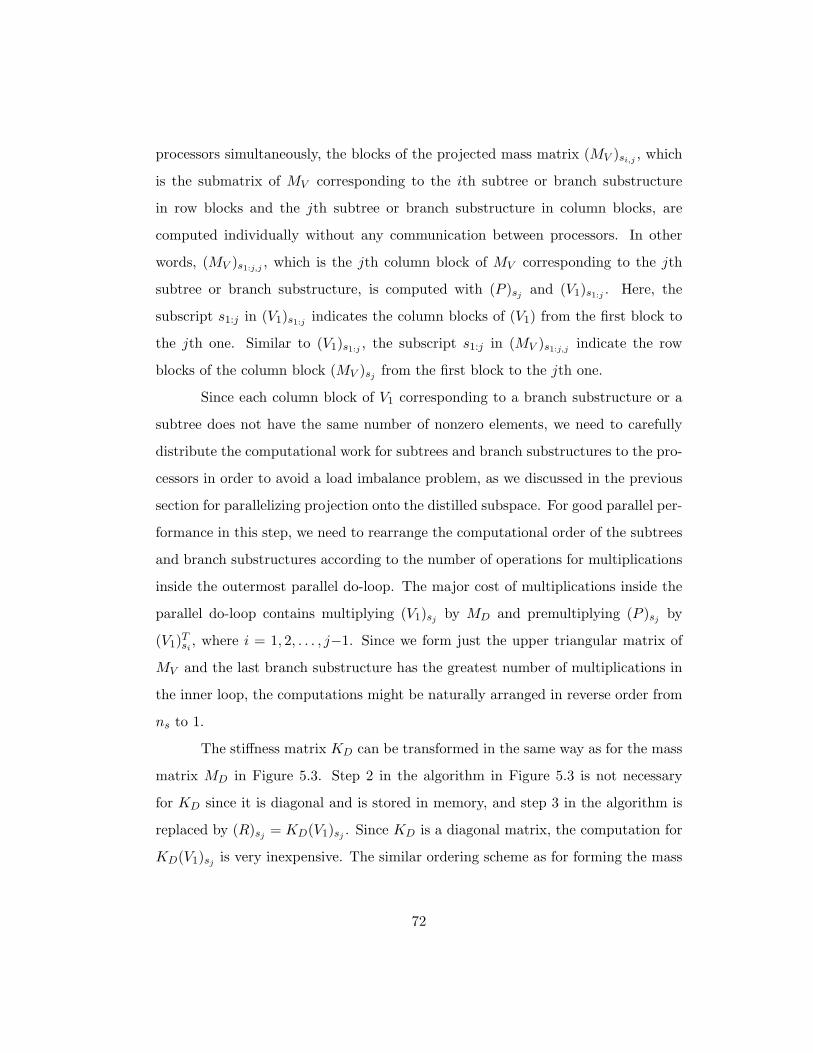
processors simultaneously, the blocks of the projected mass matrix (MV )si,j , which

is the submatrix of MV corresponding to the ith subtree or branch substructure

in row blocks and the jth subtree or branch substructure in column blocks, are

computed individually without any communication between processors. In other

words, (MV )s1:j,j , which is the jth column block of MV corresponding to the jth

subtree or branch substructure, is computed with (P )sj and (V1)s1:j . Here, the

subscript s1:j in (V1)s1:j indicates the column blocks of (V1) from the first block to

the jth one. Similar to (V1)s1:j , the subscript s1:j in (MV )s1:j,j indicate the row

blocks of the column block (MV )sj from the first block to the jth one.

Since each column block of V1 corresponding to a branch substructure or a

subtree does not have the same number of nonzero elements, we need to carefully

distribute the computational work for subtrees and branch substructures to the pro-

cessors in order to avoid a load imbalance problem, as we discussed in the previous

section for parallelizing projection onto the distilled subspace. For good parallel per-

formance in this step, we need to rearrange the computational order of the subtrees

and branch substructures according to the number of operations for multiplications

inside the outermost parallel do-loop. The major cost of multiplications inside the

parallel do-loop contains multiplying (V1)sj by MD and premultiplying (P )sj by

(V1)Tsi

, where i = 1, 2, . . . , j−1. Since we form just the upper triangular matrix of

MV and the last branch substructure has the greatest number of multiplications in

the inner loop, the computations might be naturally arranged in reverse order from

ns to 1.

The stiffness matrix KD can be transformed in the same way as for the mass

matrix MD in Figure 5.3. Step 2 in the algorithm in Figure 5.3 is not necessary

for KD since it is diagonal and is stored in memory, and step 3 in the algorithm is

replaced by (R)sj = KD(V1)sj . Since KD is a diagonal matrix, the computation for

KD(V1)sj is very inexpensive. The similar ordering scheme as for forming the mass

72

matrix MV can be applied for forming KV .

5.2.2 Parallelism for Solving the Projected Eigenproblem on Ritz

Subspace

In the second phase in Rayleigh-Ritz analysis, which is for solving the projected

eigenproblem on the Ritz subspace, there are four steps as shown in Figure 4.6:

(1) Cholesky factorization of the mass matrix MV , (2) transforming the generalized

eigenproblem to a standard form by forming the matrix AV = U−T KV U−1 using

the Cholesky factor of MV = UT U , (3) solving the dense standard eigenproblem

AV XV = XV ΛV , and (4) backtransforming the eigensolution for the standard eigen-

problem to that of the generalized eigenproblem. In step (3), there are also three

subphases as we discussed in Chapter 4. The implementation for the tridiagonal

eigensolution is very fast due to the O(nV

2) algorithm by Dhillon [63]. For example,

solving a tridiagonal eigenproblem of order 9708 takes only 32 seconds on a single

processor for the Full-Vehicle model that we used at the beginning of this chapter

to demonstrate sequential performance of the new algorithm implementation. So

there is little motivation to parallelize the routine DSTEGR in LAPACK. In ad-

dition, the Householder reduction to tridiagonal form and the backtransformation

have been parallelized with the OpenMP API by C. W. Kim [65]. Therefore, the

parallelization of the Householder eigensolution process in step 3 is not within the

scope of this dissertation, so the performance will only be checked in Chapter 6.

Cholesky factorization in step 1 in Figure 4.6 can be easily parallelized us-

ing OpenMP. For good parallel performance, the best sequential block version of a

left-looking algorithm, which is used in DPOTRF of LAPACK, is modified for par-

allelization as shown in Figure 5.4. Here we assume that the full symmetric matrix

MV is evenly partitioned with an optimal blocksize which is computed by DLAENV

in LAPACK, so that (MV )i,j represents the submatrix corresponding to the ith row

73

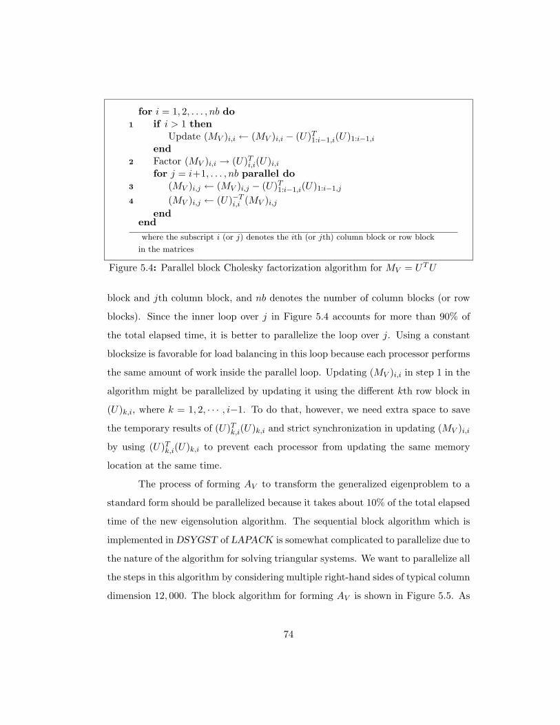
for i = 1, 2, . . . , nb do

1 if i > 1 then

Update (MV )i,i ← (MV )i,i − (U)T1:i−1,i(U)1:i−1,i

end

2 Factor (MV )i,i → (U)Ti,i(U)i,i

for j = i+1, . . . , nb parallel do

3 (MV )i,j ← (MV )i,j − (U)T1:i−1,i(U)1:i−1,j

4 (MV )i,j ← (U)−Ti,i (MV )i,j

endend

where the subscript i (or j) denotes the ith (or jth) column block or row block

in the matrices

Figure 5.4: Parallel block Cholesky factorization algorithm for MV = UT U

block and jth column block, and nb denotes the number of column blocks (or row

blocks). Since the inner loop over j in Figure 5.4 accounts for more than 90% of

the total elapsed time, it is better to parallelize the loop over j. Using a constant

blocksize is favorable for load balancing in this loop because each processor performs

the same amount of work inside the parallel loop. Updating (MV )i,i in step 1 in the

algorithm might be parallelized by updating it using the different kth row block in

(U)k,i, where k = 1, 2, · · · , i−1. To do that, however, we need extra space to save

the temporary results of (U)Tk,i(U)k,i and strict synchronization in updating (MV )i,i

by using (U)Tk,i(U)k,i to prevent each processor from updating the same memory

location at the same time.

The process of forming AV to transform the generalized eigenproblem to a

standard form should be parallelized because it takes about 10% of the total elapsed

time of the new eigensolution algorithm. The sequential block algorithm which is

implemented in DSYGST of LAPACK is somewhat complicated to parallelize due to

the nature of the algorithm for solving triangular systems. We want to parallelize all

the steps in this algorithm by considering multiple right-hand sides of typical column

dimension 12, 000. The block algorithm for forming AV is shown in Figure 5.5. As

74

for i = 1, 2, . . . , nb do

1 (AV )i,i ← (U)−Ti,i (AV )i,i(U)−1

i,i

2 for j = i+1, . . . , nb parallel do

(AV )i,j ← (U)−Ti,i (AV )i,j

(AV )i,j ← (AV )i,j − 12(AV )i,i(U)i,j

end

3 Parallel rank-2k update :for j = i+1, . . . , nb parallel do

for k = i+1, . . . , j do

(AV )k,j ← (AV )k,j − (AV )Ti,k(U)i,j − (U)T

i,k(AV )i,j

endend

4 for j = i+1, . . . , nb parallel do

(AV )i,j ← (AV )i,j − 12(AV )i,i(U)i,j

end

5 for k = 1, . . . , nrb parallel do

(AV )ik,i+1:nb ← (AV )ik,i+1:nb(U)−1i+1:nb,i+1:nb

endend

Figure 5.5: Parallel block algorithm for forming AV = U−T KV U−1

shown in the algorithm, there are five steps for parallelization. The first step is to

form (AV )i,i using an unblocked algorithm. The second step is to update (AV )i,j

over j (= i + 1, . . . , nb) for the given ith block, which can be parallelized by letting

each processor work on a different column block of (AV )i,i+1:nb. The third step is to

update the upper triangular part of (AV )i+1:nb,i+1:nb, which is a symmetric rank-2k

update. This step takes almost 65% of the total elapsed time of this algorithm.

This symmetric rank-2k update, consisting of two matrix-matrix multiplications,

can be easily parallelized by letting each processor work on a different column block

of (AV )i+1:nb,i+1:nb, using different column blocks of (U)i,i+1:nb and (AV )i,i+1:nb.

As the fourth step, (AV )i,j blocks are updated again, similar to the second line

in step 2 and this step can be parallelized over each column block j. The fifth

step is to solve a triangular system for multiple right-hand sides. In this step,

(AV )i,i+1:nb is partitioned into nrb row blocks and each processor performs the

75

operation (AV )ik,i+1:nb(U)−1i+1:nb,i+1:nb by calling a serial version of a triangular solver

for multiple right-hand sides. Here, (AV )ik,i+1:nb represents kth row block within

ith row block of AV .

To parallelize the backtransformation of the eigenvectors of the standard

form to those of the generalized eigenproblem in step 4 in Figure 4.6, we simply

divide the XV matrix into several column blocks and parallelize the computation

of solving a triangular system U(QV )j = (XV )j for (QV )j . Here, (XV )j and (QV )j

are the jth column block of XV (∈ RnV×nE) and QV (∈ R

nV×nE), respectively, and

U (∈ RnV×nV) is an upper triangular matrix which is the Cholesky factor of MV .

Each processor solves a triangular system with a block of multiple right hand sides

in XV by calling the optimized single processor version of the triangular solver. We

can take different parallelism for this backtransformation, for example, parallelizing

the loop of the triangular-solve process. However, that approach is not good for our

case because we have typically 12, 000 vectors on the right-hand side.

5.2.3 Parallelism for Computing the Ritz Eigenvectors

Computing the Ritz eigenvectors, ΦD = V1QV , using the Ritz subspace matrix V1

and the matrix QV of eigenvectors of the Rayleigh-Ritz eigenproblem, requires a

reduction operation in parallel implementation. A sum of a global variable that can

be computed by collecting local data from processors is an example of a reduction

operation. The multiplication V1QV can be done by the subtrees and the branch

substructures as

ΦD = V1QV =[

(V1)s3(V1)s6

(V1)s7

]

QV s3

QV s6

QV s7

= (V1)s3QV s3

+ (V1)s6QV s6

+ (V1)s7QV s7

(5.1)

76

Make a priority list for subtrees and branch substructuresfor j = 1, 2, . . . , nb do

Read in (QV )j

Allocate and initialize (VT )k for k processorsfor i = 1, 2, . . . , ns parallel do

Select si from the priority listRead in (V1)si

1 (VT )k = (VT )k + (V1)si(QV )j

end

Initialize (ΦD)j

for k = 0, 1, . . . , (nproc−1) do

2 (ΦD)j = (ΦD)j + (VT )k ←− implicit reduction operationend

Write out (ΦD)j

end

Figure 5.6: Parallel algorithm for computing Ritz eigenvectors in Rayleigh-Ritz analysis

In Equation (5.1), using the simple plate model as used in Chapter 4, the matrix QV

is partitioned into three row blocks corresponding to two subtrees and one branch

substructure. Similarly, the matrix V1 is partitioned into three column blocks. The

final product ΦD can be computed by summing the results of (V1)siQV si, where

i = 3, 6, and 7.

Figure 5.6 shows the parallel algorithm for computing the Ritz eigenvectors.

The multiplication of the jth full column block (QV )j by the sparse column block

(V1)si , corresponding to the ith subtree or branch substructure, can be assigned to

the kth processor, so that this processor performs the multiplication (V1)si(QV )j

and overwrites the result into its temporary memory space (VT )k. Then, the final

result can be computed by summing the results of multiplications (VT )k from all the

processors. Here, QV is also partitioned into nb column blocks to save the memory

usage because QV might fit into memory but ΦD does not fit into memory due to

its excessive size, which is typically larger than 3.0 gigabytes.

Since the numbers of non-zero elements in the column blocks of V1, corre-

77

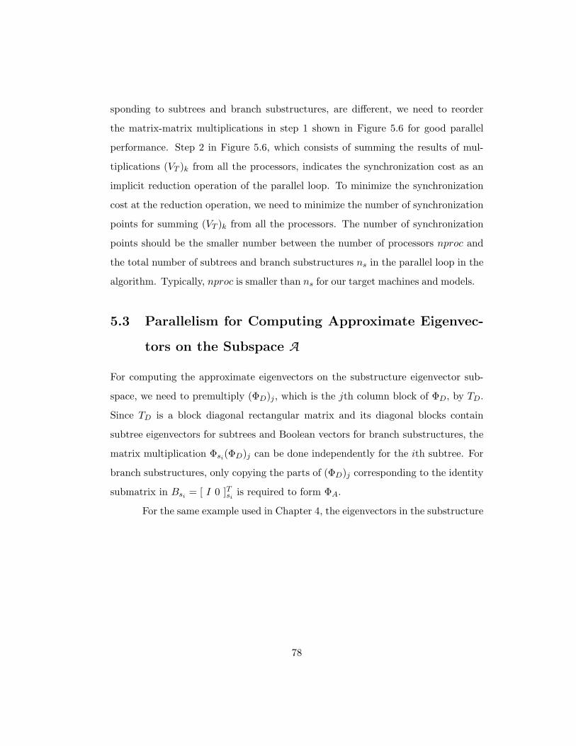
sponding to subtrees and branch substructures, are different, we need to reorder

the matrix-matrix multiplications in step 1 shown in Figure 5.6 for good parallel

performance. Step 2 in Figure 5.6, which consists of summing the results of mul-

tiplications (VT )k from all the processors, indicates the synchronization cost as an

implicit reduction operation of the parallel loop. To minimize the synchronization

cost at the reduction operation, we need to minimize the number of synchronization

points for summing (VT )k from all the processors. The number of synchronization

points should be the smaller number between the number of processors nproc and

the total number of subtrees and branch substructures ns in the parallel loop in the

algorithm. Typically, nproc is smaller than ns for our target machines and models.

5.3 Parallelism for Computing Approximate Eigenvec-

tors on the Subspace A

For computing the approximate eigenvectors on the substructure eigenvector sub-

space, we need to premultiply (ΦD)j , which is the jth column block of ΦD, by TD.

Since TD is a block diagonal rectangular matrix and its diagonal blocks contain

subtree eigenvectors for subtrees and Boolean vectors for branch substructures, the

matrix multiplication Φsi(ΦD)j can be done independently for the ith subtree. For

branch substructures, only copying the parts of (ΦD)j corresponding to the identity

submatrix in Bsi = [ I 0 ]Tsiis required to form ΦA.

For the same example used in Chapter 4, the eigenvectors in the substructure

78

Make a priority list for subtrees and branch substructuresfor j = 1, 2, . . . , nb do

Read in (ΦD)j

Initialize (ΦA)j

for i = 1, 2, . . . , ns parallel do

Select si from the priority listif si is subtree then

Read in Φsi

(ΦA)j = Φsi(ΦD)j

else

(ΦA)j = Bsi(ΦD)j

endend

Write out (ΦA)j

end

Figure 5.7: Parallel algorithm for computing approximate eigenvectors onthe substructure eigenvector subspace (A)

eigenvector subspace can be given by

ΦA ≈ TDΦD =

Φs30 0

0 Φs60

0 0 Bs7

ΦDs3

ΦDs6

ΦDs7

=

Φs3ΦDs3

Φs6ΦDs6

Bs7ΦDs7

(5.2)

The row blocks of ΦA corresponding to subtrees and branch substructures can be

formed independently by multiplying ΦDsiby Φsi for subtrees and by copying a part

of ΦDsifor branch substructures. Therefore, each processor updates a different row

block of ΦA without any communication between processors. The parallel algorithm

of this process is shown in Figure 5.7.

Since each subtree eigenvector matrix Φsi has a different size, the order of

parallel computations should be carefully organized to avoid waiting for synchro-

nization at the end of the parallel do-loop in Figure 5.7. The dynamic scheduling

79

should be used in order to efficiently distribute subtree eigenvectors to all the pro-

cessors, and the reordering of the computation of Φsi(ΦD)j must be done carefully

based on the size of the subtree eigenvectors to avoid unnecessary idle times of the

processors. Note that the column blocksize for ΦD should be set large enough to

avoid multiple readings of subtree eigenvectors represented by Φsi , but small enough

to avoid large memory usage.

80

Chapter 6

Numerical Results and

Performance

In this chapter, three FE models developed by the automotive industry are used as

test cases for the new algorithm presented in Chapter 4 and Chapter 5. Here we

focus on practical applications from the automotive industry as the main driving

force behind this new eigensolver design. The first two models have around 2 million

FE degrees of freedom (DOF), which has been a typical dimension of FE models

of car bodies in recent years. However, their modal densities, which are of greater

importance to the eigensolution algorithm, are very different. The first model has

4,216 modes below the user-specified cutoff frequency, and the second model has

7,451 modes below the user-specified cutoff frequency. The third model has 8.4 mil-

lion FE DOF and more than 11,000 modes below the user-specified cutoff frequency,

and was recently developed in the automotive industry for practical structural anal-

ysis. It has been used for benchmarking computer software and hardware in the

automotive industry. This is the most challenging model of the three for the AMLS

software, not only because this model has a large number of FE degrees of freedom,

but also because this model has so many modes.

81

For each FE model, the frequency range of interest is defined by the analyst

for modal frequency response analysis, which requires a partial eigensolution of the

FE model. It is obviously important to maintain good accuracy of approximate

natural frequencies up to the highest excitation frequency ωF, because the natural

frequencies below ωF determine the locations of peaks in the frequency response

function [48]. Approximate natural frequencies should be accurate at least to within

a relative error of 0.01 compared to the exact natural frequencies of the system.

The global cutoff frequency for natural frequencies computed in the eigensolution is

denoted by ωG. Following standard practice in the automotive industry [69], we use

the value ωG = 1.5 ωF for all the models in this chapter, for good accuracy in the

modal frequency response analysis.

We will use two of the models to determine operational parameters for the

new eigensolution algorithm described in the previous two chapters, for achieving

near-optimal performance with acceptable accuracy. The third model is used to

demonstrate the performance of Phase4 for the models of our target size, which have

about 10M FE degrees of freedom, 100K substructure modes, and 10K eigenpairs

below an user-defined cutoff frequency. The performance and accuracy of the new

eigensolution algorithm implementation will be compared to that of the shift-invert

block Lanczos eigensolver as implemented in the commercial software MSC.Nastran

(version 2001). From results obtained for the “8.4M DOF” model, we will show

that this new eigensolution algorithm, used within AMLS, significantly extends the

capability of solving eigenproblems for large structural systems with high modal

density, since solving this problem using any existing eigensolver is not practical,

particularly on microprocessor-based computer hardware.

There are several operational parameters affecting the eigensolution accu-

racy in the new eigensolution algorithm, as explained in Chapter 4. Our goal for

choosing optimal parameter values is to minimize the computational cost for solving

82

a variety of practical eigenproblems while satisfying the minimum requirements on

eigensolution accuracy. For this parameter optimization for our complex algorithm,

it is hard to quantify the objective functions for performance indices, like elapsed

time, memory usage, disk usage, and amount of data transferred. In addition, there

are tradeoffs among those performance indices. For example, bigger disk space and

larger amount of data transferred are required to reduce maximum memory usage,

while increasing total elapsed time due to increased amount of I/O. During the

course of developing this new eigensolution algorithm, we have learned a great deal

about the factors that are important to its performance, although not in a very

predictable or systematic manner. So, near-optimal parameter values for various

industrial problems have been found. However, it is still worthwhile to examine the

effect of each parameter in turn, to understand the sensitivity of each parameter.

Based on the near-optimal values of the parameters resulting from the initial opti-

mization study, we will present a detailed discussion of the effects of the parameters,

moving sequentially from the most impacting parameter to the least, for the next

two industrial models.

Performance is primarily measured in terms of elapsed time, memory usage,

disk usage, and data transfer. Elapsed time is the most important performance

metric for large-scale industrial vibration analysis since the most important practical

objective is to reduce job turnaround time. We will express the elapsed time either in

seconds (sec.) or in hours, minutes, and seconds (hh:mm:ss) as appropriate. Memory

usage is simply the maximum amount of physical memory used during the execution

of the program. If a program or algorithm requires too much memory, this limits

the size of jobs that can be run on a given hardware platform. Disk usage is the

maximum amount of disk space used during the execution of the program. If the

amount of disk space required exceeds the capacity of physical disk storage, it is

impossible to run the program. Data transfer is the amount of data that is either

83

read in or written out by the program during the execution of the program. If

the program requires excessive amounts of data to be transferred between disk and

memory, this data transfer creates a performance bottleneck since the CPU has to

wait for data to be read from or written to disk.

Accuracy is evaluated by comparing the results produced by the new eigenso-

lution algorithm with those obtained using the block Lanczos eigensolver in MSC.Nas-

tran. The accuracy of eigenvalues will be measured in two ways: (1) relative error of

the natural frequencies computed by Phase4, which are the square roots of approx-

imate eigenvalues, compared with the natural frequencies computed by the block

Lanczos eigensolver, and (2) the number of approximate natural frequencies found

below the global cutoff frequency. Since the Rayleigh-Ritz approximate eigenvalues

computed by the new eigensolver provide upper bounds to the exact eigenvalues,

the approximate eigenvalues, especially those close to the global cutoff value ωG

2,

are shifted to values slightly higher than the exact ones. Hence, we would not ob-

tain as many eigenvalues below the cutoff value as the exact number of eigenvalues

below the cutoff value. The number of approximate eigenvalues found is related to

the accuracy of the frequency response function. Therefore, we will require that

the number of approximate eigenvalues below the global cutoff value ωG

2 should be

more than 99.5% of the number of actual eigenvalues below the global cutoff value

on the substructure eigenvector subspace.

The quality of the set of approximate eigenvectors can be evaluated by com-

puting the principal angles between subspaces containing (virtually) “exact” eigen-

vectors and the approximate ones [45, 46, 62]. This is done by computing the

singular value decomposition of ΦTLMAΦA, where ΦL is a matrix containing eigen-

vectors computed by the block Lanczos eigensolver in MSC.Nastran, ΦA is a matrix

containing the approximate eigenvectors computed by Phase4, and MA is the AMLS

transformed mass matrix. If the eigenvectors are nearly equal, the singular values,

84

Figure 6.1: Finite element representation of Trim-Body model

which equal the cosines of the principal angles between the two eigenspaces, will be

close to unity.

Performance was evaluated on an HP rx5670 server containing four 900 MHz

IA-64 (Itanium2) processors. This is a shared memory machine which has 8 giga-

bytes (GB) of physical memory and 500 GB of disk space. The operating system is

HP-UX version B.11.22.

The new eigensolution algorithm was implemented primarily in Fortran90,

with C for I/O. As was mentioned at the beginning of this dissertation, the new

algorithm is designed for solving the reduced eigenvalue problem that AMLS pro-

duces, so the computer implementation is a part of the commercial AMLS software

package.

85

6.1 Trim-Body Model

The first model is a “trim body” model that has 1.58 million FE degrees of freedom.

A trim body model is a model of a car body that has a steering mechanism, moving

parts (doors, hood, trunk lid), and seats. As shown in Figure 6.1, this model

represents the cab of a full size truck without any parts of the truck behind the cab.

We will refer to this model as the Trim-Body model. There are three forced degrees

of freedom for this model, which can be used for residual flexibility computation as

explained in Appendix A. The number of “output” degrees of freedom requested by

the user is 116, so the frequency response is computed for only 116 selected degrees

of freedom.

The frequency range of interest for frequency response analysis is from zero

to 400 Hz. Since the highest excitation frequency of interest for frequency response

analysis is 400 Hz, the cutoff for natural frequencies of global modes used in the

modal frequency response analysis is 600 Hz for this model. The cutoff frequency

for the substructure eigenvalue problems is set to 3,000 Hz, which is five times

as high as the global cutoff frequency. Throughout this chapter, we will use the

value 5.0 as the default for the ratio ωA/ωG between substructure and global cutoff

frequencies.

Since Phase4 is a part of the AMLS software, its performance is affected by

the results of Phase2 and Phase3. The numerical results of Phase2 and Phase3 are

explained below, and the performance results of Phase2 and Phase3 are summarized

in Table 6.1. Phase2 of the AMLS software automatically divides this model into

4,121 substructures on 22 levels. The substructure tree is shown in Figure 4.4(a) in

Chapter 4. The substructure sizes range up to 1,500 degrees of freedom based on the

target size of 1,500 for leaf substructures, and 1,000 for branch substructures, which

are substructures having descendant substructures in the substructure tree. Phase2

performance is not related to any specified excitation or cutoff frequencies, because

86

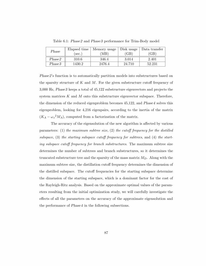
Table 6.1: Phase2 and Phase3 performance for Trim-Body model

PhaseElapsed time Memory usage Disk usage Data transfer

(sec.) (MB) (GB) (GB)

Phase2 310.6 346.4 3.014 2.401

Phase3 1430.2 2476.4 24.710 52.231

Phase2’s function is to automatically partition models into substructures based on

the sparsity structure of K and M . For the given substructure cutoff frequency of

3,000 Hz, Phase3 keeps a total of 45,122 substructure eigenvectors and projects the

system matrices K and M onto this substructure eigenvector subspace. Therefore,

the dimension of the reduced eigenproblem becomes 45,122, and Phase4 solves this

eigenproblem, looking for 4,216 eigenpairs, according to the inertia of the matrix

(KA − ωG

2MA), computed from a factorization of the matrix.

The accuracy of the eigensolution of the new algorithm is affected by various

parameters: (1) the maximum subtree size, (2) the cutoff frequency for the distilled

subspace, (3) the starting subspace cutoff frequency for subtrees, and (4) the start-

ing subspace cutoff frequency for branch substructures. The maximum subtree size

determines the number of subtrees and branch substructures, so it determines the

truncated substructure tree and the sparsity of the mass matrix MD. Along with the

maximum subtree size, the distillation cutoff frequency determines the dimension of

the distilled subspace. The cutoff frequencies for the starting subspace determine

the dimension of the starting subspace, which is a dominant factor for the cost of

the Rayleigh-Ritz analysis. Based on the approximate optimal values of the param-

eters resulting from the initial optimization study, we will carefully investigate the

effects of all the parameters on the accuracy of the approximate eigensolution and

the performance of Phase4 in the following subsections.

87

Table 6.2: Effect of maximum subtree size on the dimension and quality of thedistilled subspace D for Trim-Body model

Maximum Number of Number of branch Dimensionν(KD − ωG

2MD)subtree size subtrees substructures of D

1000 63 62 28674 4212

2000 33 34 27873 4213

3000 23 24 27503 4214

4000 19 20 27240 4214

5000 14 15 26965 4215

6000 13 14 26901 4215

7000 8 10 26740 4215

6.1.1 Effect of Maximum Subtree Size

The maximum subtree size is used to define the terminal subtrees for the given

substructure tree. As discussed in Chapter 4, a subtree is formed by merging sub-

structures together starting at the leaf nodes of the substructure tree as long as the

number of accumulated substructure eigenvectors does not exceed the maximum

subtree size. To see the effect of the maximum subtree size, we set the other three

parameters to their approximate optimal values for this model. The approximate op-

timal values for these parameters are: ωD = 0.8 ωA, ωst

V= 1.1 ωG, and ωbs

V= 1.7 ωG.

If more than 4,195 eigenvalues out of 4,216 below the global cutoff are found by

the new eigensolution algorithm, we consider the approximate eigensolution to have

achieved acceptable accuracy.

An increase in the maximum subtree size decreases the total number of

subtrees and branch substructures and the dimension of the distilled subspace, as

shown in Table 6.2. However, it increases the accuracy in terms of the number of

actual eigenpairs below the global cutoff value on the distilled subspace. In Ta-

ble 6.2, ν(KD − ωG

2MD) denotes the number of negative eigenvalues of the matrix

(KD−ωG

2MD), which is the same as the number of the actual eigenvalues below the

cutoff value, ωG

2, for the generalized eigenvalue problem KDΦD = MDΦDΛD. The

88

Table 6.3: Effect of maximum subtree size on the eigensolution accuracy and per-formance of Phase4 for Trim-Body model

Maximum Dimension Number of nE/nV Phase4

subtree size of V0 (nV) eigenpairs (nE) (%) elapsed time (sec.)

1000 6624 4181 63.1 1233.3

2000 6180 4190 67.7 1146.8

3000 5956 4195 70.4 1189.7

4000 5792 4199 72.4 1378.4

5000 5623 4202 74.7 1746.3

6000 5581 4203 75.3 1938.3

7000 5484 4204 76.6 2639.2

number of actual eigenvalues below the global cutoff value on the distilled subspace

does not change for the cases using maximum subtree sizes of more than 5,000.

This indicates that increasing the maximum subtree size to more than 5,000 does

not affect on the eigensolution accuracy below the global cutoff value on the distilled

subspace with the near-optimal values of the other parameters.

Table 6.3 shows the effect of the maximum subtree size on the eigensolution

accuracy and performance of Phase4 for this model. Because the eigenproblem on

the distilled subspace D is only solved approximately, the number of approximate

eigenpairs found is less than the number of exact eigenvalues below the global cutoff

value determined by ν(KD − ωG

2MD). Since we need more than 4,195 eigenpairs

below the global cutoff value for acceptable accuracy, using a maximum subtree

size of more than 3,000 results in acceptable eigensolution accuracy for this model.

However, as the maximum subtree size increases, the rate of increase in the number

of approximate eigenvalues, diminishes and eventually stops for maximum subtree

sizes of more than 5,000. Using a maximum subtree size of more than 6,000 has

little benefit on the accuracy of the eigensolution, but degrades the timing perfor-

mance significantly with only a small improvement in “computational efficiency of

the Rayleigh-Ritz analysis”, (nE/nV), where nE is the number of eigenpairs found by

89

the new eigensolution algorithm and nV is the dimension of the starting subspace.

Here, the computational efficiency of the Rayleigh-Ritz analysis is considered as one

minor factor that determine the near-optimal performance of Phase4 because the

goal of the new eigensolution algorithm is to minimize the total computational cost

by maximizing the efficiency of the Rayleigh-Ritz analysis.

Solving subtree eigenproblems accounts for a large proportion of the total

elapsed time in Phase4 for this model, which will be shown in a later subsection.

Since the subtree eigenproblems are solved by using Householder reduction to tridi-

agonal form, the cost of solving a subtree eigenproblem is proportional to the cube

of the dimension of the subtree eigenproblem. Since we need approximately 45%

of the eigenpairs for a subtree problem based on the near-optimal distillation cut-

off frequency ωD, an eigensolution algorithm suitable for full eigensolution of dense

problems is likely to perform better than the block Lanczos method for subtree

eigenproblems of small dimension. However, the block Lanczos method could be

faster for subtree eigenproblems of large dimension if a smaller percentage of the

eigenpairs were needed.

Figure 6.2 illustrates the effect of various maximum subtree sizes on the

relative error of the approximate natural frequencies compared to the natural fre-

quencies computed by the block Lanczos eigensolver on the substructure eigenvector

subspace (A). The relative errors of the natural frequencies for all the cases up to

the frequency 600 Hz, are less than 0.01. Moreover, the relative error of the natural

frequencies less than 400 Hz, which is the highest excitation frequency, is less than

0.001 for all the cases. For this model, we conclude that the maximum subtree size of

5,000 is nearly optimal when both accuracy and timing performance are considered.

90

0 100 200 300 400 500 60010

−10

10−9

10−8

10−7

10−6

10−5

10−4

10−3

10−2

10−1

Frequency (Hz)

Rel

ativ

e E

rro

r

1000 3000 5000 7000

Figure 6.2: Effect of maximum subtree size on the accuracy of the natural frequenciesby Phase4 for Trim-Body model

6.1.2 Effect of the Distillation Cutoff Frequency

For this model, along with the fixed maximum subtree size of 5,000, which results

in 14 subtrees and 15 branch substructures, the distillation cutoff frequency, ωD,

determines the dimension of the distilled subspace. The substructure eigenvector

subspace is distilled by solving subtree eigenproblems and truncating the subtree

eigenspaces, and by simply truncating eigenspaces for branch substructures based

on the distillation cutoff frequency ωD. For dimensional reduction of the given

substructure eigenvector subspace, the distillation cutoff frequency should be less

than or equal to the substructure cutoff frequency ωA.

91

Table 6.4: Effect of the distillation cutoff frequency ωD for Trim-Body model

ωD/ωA Dimensionν(KD − ωG

2MD)Dimension Number of Phase4

ratio of D of V0 eigenpairs elapsed time

0.2 4686 3992 4550 3992 758.6 sec.

0.3 8124 4170 5435 4158 986.0 sec.

0.4 11802 4197 5556 4184 1135.3 sec.

0.5 15632 4209 5575 4194 1265.7 sec.

0.6 19515 4212 5591 4198 1420.9 sec.

0.7 23363 4214 5607 4200 1554.7 sec.

0.8 26965 4215 5623 4202 1747.6 sec.

0.9 30267 4215 5633 4203 1872.7 sec.

1.0 32954 4215 5640 4203 1985.6 sec.

Table 6.4 summarizes the effect of various distillation cutoff frequencies. Note

that the substructure cutoff frequency ωA is 5.0 ωG, and so ωD = 0.2 ωA = ωG is

a lower bound for ωD, because a good global eigensolution accuracy can not be

expected with a lower cutoff for subtree eigenproblems and branch substructure

eigenspaces. As ωD increases, the dimension of the distilled subspace grows rapidly,

but the number of negative eigenvalues of the matrix (KD − ωG

2MD) increases

quickly at first and stops increasing after ωD = 0.8 ωA. Considering the require-

ment of computing 99.5% (4195) of the number of eigenvalues below the global

cutoff value, the cases with ωD higher than 0.6 ωA generate acceptable approximate

eigensolutions. However, there is little benefit on the eigensolution accuracy from

increasing ωD beyond 0.8 ωA because the number of eigenvalues below the global

cutoff value is improved little while elapsed time increases dramatically. The num-

ber of eigenvalues below ωG

2 for the matrix pencil (KD, MD), as determined by the

inertia of (KD − ωG

2MD), is not improved.

The elapsed time for each case in Table 6.4 shows the cost of increasing the

distillation cutoff frequency. The cost of increasing the distillation cutoff frequency

ωD is associated with projecting system matrices KA and MA onto the distilled

92

0 100 200 300 400 500 60010

−10

10−9

10−8

10−7

10−6

10−5

10−4

10−3

10−2

10−1

Frequency (Hz)

Rel

ativ

e E

rro

r

0.2 ωA

0.4 ωA

0.6 ωA

0.8 ωA

1.0 ωA

Figure 6.3: Effect of the distillation cutoff frequency ωD on the accuracy of theapproximate natural frequencies for Trim-Body model

subspace and expanding approximate eigenvectors on the distilled subspace to those

on the substructure eigenvector subspace in the algorithm shown in Figure 4.1. If

we collect many eigenvectors for subtrees and branch substructures by increasing

the value of ωD, the dimension of the distilled subspace grows quickly and so does

the cost of computations using subtree eigenvectors.

The relative errors of the approximate natural frequencies computed by

Phase4 for five different values of ωD, with respect to the (virtually exact) natural

frequencies computed by the block Lanczos eigensolver for the reduced eigenproblem

on the subspace A , are shown in Figure 6.3. The distillation cutoff frequency ωD

93

has a strong effect on the accuracy of approximate natural frequencies. The relative

errors of the natural frequencies below the global cutoff frequency (ωG = 2π ·600 Hz)

for all the cases except for ωD = 0.2 ωA = ωG, are less than 0.01. Below the highest

excitation frequency, 400 Hz, the relative errors of the natural frequencies for the

cases in which ωD ≥ 0.6 ωA, are less than 0.001. Therefore, ωD = 0.8 ωA is chosen

as a near-optimal value for this model based on acceptable accuracy and affordable

timing performance.

6.1.3 Effect of Starting Subspace Cutoff Frequencies

In Chapter 4, two cutoff frequencies were introduced in forming a starting subspace

in the distilled subspace (D). One is ωst

Vfor subtrees and the other is ωbs

Vfor branch

substructures. These starting subspace cutoff frequencies determine the dimension

of the starting subspace, which is a decisive factor for the cost of the Rayleigh-Ritz

analysis. We need to determine near-optimal values for these two cutoff frequencies

based on the numerical experiments that follow.

Throughout this section, the effect of the starting subspace cutoff frequencies

is examined by assuming the dimension and quality of the distilled subspace have

been determined by setting the maximum subtree size to 5,000 and the distillation

cutoff frequency ωD to 0.8 ωA. Table 6.5 shows the effect of various choices of ωst

V

along with the fixed ωbs

V= 1.7 ωG. As ωst

Vincreases, the dimension of the starting sub-

space increases rapidly, but the number of approximate eigenvalues below the global

cutoff value increases slowly and stops increasing for the cases for which ωst

V≥ 1.3 ωG.

Considering the requirement of computing more than 4,195 approximate eigenpairs,

the values of ωst

Vgreater than 1.1 ωG satisfy this requirement. On the other hand,

as ωst

Vincreases, the elapsed time and the maximum memory usage for the cases for

which ωst

V≥ 1.1 ωG increase without significant accuracy improvement. Therefore,

ωst

V= 1.1 ωG shows the best timing performance and the best ratio (74.6%) of the

94

Table 6.5: Effect of starting subspace cutoff frequency ωst

Vfor subtrees for Trim-Body

model

ωst

V/ωG Dimension Number of nE/nV Phase4

ratio of V0 eigenpairs (%) timing (sec.) memory (MB)

1.0 5027 4141 82.3 1604.8 455.8

1.1 5629 4202 74.6 1746.3 553.5

1.2 6249 4211 67.3 1859.1 665.8

1.3 6886 4213 61.1 2005.1 793.4

1.4 7539 4213 55.8 2189.4 937.0

0 100 200 300 400 500 60010

−10

10−9

10−8

10−7

10−6

10−5

10−4

10−3

10−2

10−1

Frequency (Hz)

Rel

ativ

e E

rro

r

1.0 ωG

1.1 ωG

1.2 ωG

1.3 ωG

1.4 ωG

Figure 6.4: Effect of starting subspace cutoff frequency ωst


accuracy of the approximate natural frequencies for Trim-Body model

95

computational efficiency of the Rayleigh-Ritz analysis among the cases for which

the requirement of computing more than 4,195 approximate eigenpairs is satisfied.

In Figure 6.4, the relative error of the approximate natural frequencies com-

puted by Phase4 is not very sensitive except at the high frequencies close to the

global cutoff frequency 600 Hz. Below the highest excitation frequency 400 Hz, the

relative errors of all the cases are less than 0.001 since the choice of ωst

Vhas little

effect on accuracy of the natural frequencies below 400 Hz. We choose ωst

V= 1.1 ωG

as a near-optimal value for this model based on the elapsed time, memory usage

and the computational efficiency of the Rayleigh-Ritz analysis.

Table 6.6 summarizes the effect of various choices of ωbs

V, setting ωst

V= 1.1 ωG.

This cutoff frequency ωbs

Vhas a much smaller effect than the cutoff frequency for

subtrees, ωst

V, on accuracy in the high frequency range close to the global cutoff fre-

quency. The dimension of the starting subspace, nV, and the number of approximate

eigenvalues, nE, increase slightly as the cutoff frequency ωbs

Vincreases by 0.2 ωG. This

cutoff frequency has an almost negligible effect on elapsed times and memory usage

of Phase4 for this model.

The relative errors of the approximate natural frequencies are not very sensi-

tive to an increase of this starting subspace cutoff frequency for branch substructures

as shown in Figure 6.5. The difference in the relative errors of the approximate natu-

ral frequencies among the cases for different cutoff frequencies ωbs

Vis most noticeable

in the frequency range from 400 Hz through 600 Hz. However, the difference is very

minor. Therefore, based on the requirement on the number of approximate eigen-

pairs we can choose any value of ωbs

Vgreater than 1.3 ωG for this model. To get the

maximum number of approximate eigenpairs below the global cutoff frequency with

affordable performance penalty and reasonable computational efficiency of Rayleigh-

Ritz analysis, we select ωbs

V= 1.7 ωG.

96

Table 6.6: Effect of starting subspace cutoff frequency ωbs

Vfor branch substructures

for Trim-Body model

ωbs


ratio of V0 eigenpairs (%) timing (sec.) memory (MB)

1.1 5328 4194 78.7 1638.4 503.4

1.3 5437 4199 77.2 1666.5 521.1

1.5 5526 4200 76.0 1688.8 536.1

1.7 5629 4202 74.6 1746.3 553.5

1.9 5711 4203 73.5 1751.1 567.8

0 100 200 300 400 500 60010

−10

10−9

10−8

10−7

10−6

10−5

10−4

10−3

10−2

10−1

Frequency (Hz)

Rel

ativ

e E

rro

r

1.1 ωG

1.3 ωG

1.5 ωG

1.7 ωG

1.9 ωG

Figure 6.5: Effect of starting subspace cutoff frequency ωbs


on relative errors of the approximate natural frequencies for Trim-Body model

97

Table 6.7: Parallel performance of Phase4 for Trim-Body model

Number of Phase4Speedup Efficiency

processors elapsed time (sec.)

1 1746 1.00 1.00

2 1032 1.69 0.85

4 721 2.42 0.60

6.1.4 Parallel Performance

Parallel performance can be measured by “speedup”, which is defined as the ratio

of elapsed time with multiple processors to single processor elapsed time. Also,

“efficiency”, which is the ratio of speedup to the number of processors used, is

used as another measure of parallel performance. Table 6.7 summarizes parallel

performance of Phase4 for the Trim-Body model on our shared memory machine

with up to 4 processors.

We have very nice speedup for 2 processors, but the speedup for 4 processors

is not as good. One of the causes for low speedup for 4 processors comes from the I/O

costs due to the large size of the problem. Since we cannot handle most of the data

in core, substantial I/O costs are the explanation for low speedup for this model. We

cannot avoid reading or writing intermediate data from or to temporary disk space

in blocks of code executed by multiple processors in parallel. As a result, the I/O in

a block of code executed by multiple processors causes multiple processors to wait

for a longer time for data to be read or written out due to the limited I/O buffer

size. Also, the necessary I/O in a block of code executed by a single processor,

becomes more dominant in the parallel performance as the number of processors

used increases.

As discussed in Chapter 5, the parallel regions of the new algorithm are

divided into three parts as shown in Table 6.8. The speedup for projection onto the

distilled subspace is not as good as we expected. One major reason for low speedup

98

Table 6.8: Timings and speedups for parallelized steps in the new eigensolutionalgorithm for Trim-Body model

StepNo. of processors

Speedup1 4

Projection onto subspace D 756 sec. 319 sec. 2.37

Rayleigh-Ritz analysis on subspace V1 685 sec. 267 sec. 2.56

Computation of eigenvectors ΦA 255 sec. 84 sec. 3.03

total 1746 sec. 713 sec. 2.44

Table 6.9: Timings and speedups of Rayleigh-Ritz analysis in the new algorithm forTrim-Body model


Speedup1 4

(a) projecting KD and MD onto V1 217 sec. 66 sec. 3.28

(b) factoring projected MV 28 sec. 8 sec. 3.50

(c) forming AV 74 sec. 26 sec. 2.84

(d) reduction to tridiagonal matrix 102 sec. 71 sec. 1.43

(e) solve tridiagonal eigenproblem 11 sec. 11 sec. 1.00

(f) backtransform to eigenvectors of AV 102 sec. 29 sec. 3.51

(g) backtransform to eigenvectors of (KV , MV ) 42 sec. 12 sec. 3.50

(h) computation of Ritz eigenvectors ΦD 97 sec. 29 sec. 3.34

total 685 sec. 267 sec. 2.56

with 4 processors is that since the data size for each subtree or branch substructure

is not the same and the number of subtrees is not a multiple of the number of

processors used, the idle time for all the processors increases.

The speedup for computing the approximate eigenvectors ΦA is quite good

because the matrix-matrix multiplication (ΦsiΦD) for subtrees can be easily par-

allelized without any communication between processors. Dynamic scheduling and

reordering of the subtrees according to the size of their eigenvectors help to improve

the parallel performance to overcome load imbalance due to the different sizes of

subtree eigenvector matrices Φsi .

99

A performance analysis for the Rayleigh-Ritz analysis is done in detail for

this model since the Rayleigh-Ritz analysis takes 38% of the total elapsed time,

and involves several steps as explained in Section 5.2. Table 6.9 shows the speedup

for each step in the Rayleigh-Ritz analysis. We have very nice speedups for steps

(a), (b), (f), (g), and (h) as shown in Table 6.9. Forming AV in step(c) shows

low speedup due to the nature of parallelizing solving a triangular system in the

algorithm as discussed in Section 5.2.2. However, the real bottleneck in the par-

allel performance for this model is the process of reduction to tridiagonal form in

step (d). More detailed explanation about parallelization with the OpenMP API of

Householder tridiagonal reduction procedure can be found in [65]. This Householder

tridiagonalization can be improved by using a different parallel algorithm [68].

6.1.5 Overall Performance and Eigensolution Accuracy

The eigensolution accuracy and the performance of the new eigensolution algorithm

are evaluated by comparing with two other algorithms for this model. The other two

algorithms are the subspace iteration (SI) method and the block Lanczos method.

In addition to these two eigensolution algorithms, the block Lanczos eigensolver was

executed for the projected eigenproblem on the distilled subspace in Equation (4.11),

to evaluate the distillation effect in terms of the eigensolution accuracy and compare

the performance of the block Lanczos method on the eigenproblem on the distilled

subspace D with the corresponding part of Phase4.

Table 6.10 summarizes the performance comparison among the implemen-

tations of three different algorithms for solving the reduced eigenproblem on the

substructure eigenvector subspace (A). The performance of Phase4 summarized

in Table 6.10 reflects a substructure cutoff frequency of 3,000 Hz, a global cutoff

frequency of 600 Hz, a distillation cutoff frequency of 2,400 Hz, a maximum subtree

size of 5,000, a starting subspace cutoff frequency for subtrees of 660 Hz, and a

100

Table 6.10: Performance comparison between Phase4 and two other algorithms onthe different subspaces for Trim-Body model

Performance metric Phase4 SI on A Lanczos on D Lanczos on A

Elapsed time 00:12:01 02:42:24 14:13:25 19:11:37

System time 00:01:36 00:08:08 02:37:54 06:03:09

Memory usage (MB) 1651 3289 2000 2000

Disk usage (GB) 9.2 5.7 5.7 8.8

Data transfer (GB) 31.1 204.3 4598.7 9188.4

No. of eigenpairs 4202 4199 4215 4216

starting subspace cutoff frequency for branch substructures of 1,020 Hz.

In Table 6.10, the performance results of the subspace iteration method on

the substructure eigenvector subspace are shown for comparison with other methods.

The solution of the reduced eigenproblem on the subspace A was approximated

by performing one subspace iteration on a truncated subspace in the subspace A

and one Rayleigh-Ritz analysis on the refined subspace in the subspace A . Here,

the truncated starting subspace in the subspace A is obtained by collecting unit

vectors each of which has a value of unity in a degree of freedom with the smallest

ratios (KA)ii/(MA)ii. The substructure truncation cutoff frequency for a starting

subspace was set to 1.5 ωG (= 2π · (900 Hz)) for this algorithm. With this cutoff

value for a starting subspace, the subspace iteration method obtains an approximate

eigensolution, after one iteration, having similar accuracy in terms of the number

of eigenpairs found (4,199) below the global cutoff value to that of the approximate

eigensolution computed by Phase4. This method is similar to the subspace iteration

method on the distilled subspace in the new eigensolution algorithm.

The “exact” eigensolution by the block Lanczos eigensolver on the substruc-

ture eigenvector subspace was obtained by solving the reduced eigenvalue problem

in Equation (2.3). We can solve a reciprocal eigenproblem in order to exploit the

sparsity of the diagonal stiffness matrix KA. However, this model has 6 rigid body

101

0 100 200 300 400 500 60010

−10

10−9

10−8

10−7

10−6

10−5

10−4

10−3

10−2

10−1

Frequency (Hz)

Rel

ativ

e E

rro

r

Phase4

Lanczos on D

SI on A

Figure 6.6: Accuracy of the approximate natural frequencies by three different al-gorithms on two different subspaces with the same global cutoff frequency 600 Hzfor Trim-Body model

modes, so it is impossible to solve the reciprocal eigenvalue problem due to the sin-

gularity of the matrix KA by the block Lanczos eigensolver in MSC.Nastran unless

the user can use a reverse communication interface, in which the user is free to ex-

press the action of the matrix on a block of vectors through a subroutine call within

Lanczos iterations [24].

The maximum memory size for the block Lanczos runs within MSC.Nas-

tran was set to 2.0 gigabytes for comparison purpose with Phase4. As shown in

Table 6.10, the difference in elapsed time between Phase4 and the block Lanczos

eigensolver on the subspace A is about a factor of 96. More than 6 hours of the total

102

elapsed time of the Lanczos run on the subspace A was spent in the reorthogonal-

ization of the Lanczos vectors with respect to the mass matrix MA. Since there was

significant I/O activity due to the high modal density and long length of Lanczos

vectors, the system time in the Lanczos run is 31.6% of the total elapsed time, but

the system time in Phase4 is just 96 seconds and is only 13.3% of the total elapsed

time. Here, the system time indicates the CPU time spent by the operating system

for the run and it mainly reflects the time spent for I/O. The Lanczos eigensolver

uses 8.8 GB of disk space and most disappointingly performs more than 9.1 ter-

abytes data transfer, which explains the substantial system time. Phase4 transfers

31.1 gigabytes of data to save memory usage during the runtime. Compared to

Phase4, the subspace iteration method on the subspace A requires more than twice

the memory usage and 6.58 times the amount of data transferred, and almost 14

times the execution time to achieve a similar level of eigensolution accuracy to that

obtained by Phase4.

Figure 6.6 shows the relative errors of the approximate natural frequencies

compared to the “exact” natural frequencies from the block Lanczos eigensolver

on the substructure eigenvector subspace. Every approximate natural frequency

from Phase4 has a relative error less than 0.0031 even though 14 fewer natural

frequencies below the global cutoff frequency are found compared to the number of

actual eigenpairs (4216) on the substructure eigenvector subspace. We should note

that the maximum relative error in the natural frequencies computed by Phase4

below 400 Hz is less than 0.34e−3 and Phase4 finds all of the 2,381 eigenpairs

whose natural frequencies are below 400 Hz.

The numerical results on the distilled subspace D computed by the block

Lanczos eigensolver show the effect of the distillation process as discussed in Chap-

ter 4. By projecting onto the subspace D, the dimension of the reduced eigenproblem

on the subspace A is reduced from 45,122 to 26,965, which is a 40% reduction. At

103

0 100 200 300 400 500 6000

0.1

0.3

0.5

0.7

0.9

1

Frequency (Hz)

Co

sin

e o

f th

e p

rin

cip

al a

ng

les

Figure 6.7: Cosines of the principal angles between two eigenspaces computed byPhase4 and the Lanczos eigensolver for Trim-Body model

the same time, the distillation process achieves an acceptable accuracy of the ap-

proximate eigensolution throughout the frequency range up to 600 Hz as shown in

Figure 6.6. The maximum relative error of the natural frequencies approximated

from the distilled subspace (D) compared to the natural frequencies approximated

from the substructure eigenvector subspace (A) by the block Lanczos eigensolver is

0.45e−3. No natural frequency within the frequency range of interest (from 0 Hz

to 400 Hz) is missed, and only one mode below the global cutoff frequency 600 Hz

is missed by the distillation process. Therefore, by the distillation process we can

obtain a smaller distilled subspace without losing much eigensolution accuracy.

To verify the accuracy of the eigenvectors approximated by Phase4, the

104

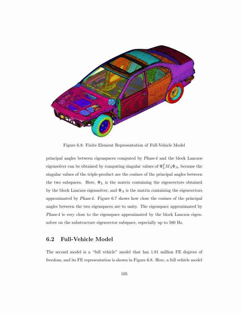
Figure 6.8: Finite Element Representation of Full-Vehicle Model

principal angles between eigenspaces computed by Phase4 and the block Lanczos

eigensolver can be obtained by computing singular values of ΦTLMAΦA, because the

singular values of the triple-product are the cosines of the principal angles between

the two subspaces. Here, ΦL is the matrix containing the eigenvectors obtained

by the block Lanczos eigensolver, and ΦA is the matrix containing the eigenvectors

approximated by Phase4. Figure 6.7 shows how close the cosines of the principal

angles between the two eigenspaces are to unity. The eigenspace approximated by

Phase4 is very close to the eigenspace approximated by the block Lanczos eigen-

solver on the substructure eigenvector subspace, especially up to 580 Hz.

6.2 Full-Vehicle Model

The second model is a “full vehicle” model that has 1.81 million FE degrees of

freedom, and its FE representation is shown in Figure 6.8. Here, a full vehicle model

105

Table 6.11: Phase2 and Phase3 performance for Full-Vehicle model

PhaseElapsed time Memory usage Disk usage Data transfer

(sec.) (MB) (GB) (GB)

Phase2 362 400.0 4.170 3.567

Phase3 2141 2189.1 34.953 50.796

denotes a car body model that has almost every part, i.e., engine, suspension, tires,

exhaust system, a steering mechanism, seats, and moving parts (door, hood, trunk

lid). We will refer to this model as the Full-Vehicle model. This model has 147 forced

degrees of freedom, and the number of “output” degrees of freedom requested by

the user is 344.

The frequency range of interest for frequency response analysis is from 0 Hz

to 500 Hz, so the highest excitation frequency ωF is 2π ·(500 Hz). For this model, the

cutoff frequency for global modes used in the modal frequency response analysis is

750 Hz. The cutoff frequency for substructure eigenproblems used in Phase3 is set

to 5.0 ωG = 2π · (3750 Hz). Again, we keep the value 5.0 as the default for the ratio

ωA/ωG between the cutoff frequency for substructure eigenproblems and the global

cutoff frequency. This model has 7 low frequency modes under 5.25 Hz. Without

handling these seven low frequency modes as explained in Section 4.8, the near linear

dependence in the subspace V1 results in unacceptable error in the eigensolution.

Phase2 of the AMLS software automatically partitions this model into 4,133

substructures on 24 levels. The substructure size ranges from 6 to 1,638 degrees

of freedom based on the target sizes of 1,500 for leaf substructures, and 1,000 for

branch substructures. For the given substructure cutoff frequency ωA, Phase3 of

the AMLS software computes 68,521 substructure eigenvectors, and projects the

system matrices K and M onto this substructure eigenvector subspace. Therefore,

the dimension of the reduced eigenproblem to be solved by Phase4 is of order

68,521 and 7,451 eigenpairs must to be found according to the inertia of the matrix

106

(KA − ωG

2MA). This model has higher modal density than the Trim-Body model

on the substructure eigenvector subspace A . The performance characteristics of

Phase2 and Phase3 are shown in Table 6.11.

The accuracy and performance of the new eigensolution algorithm is affected

by four parameters as discussed in the section for the Trim-Body model. To in-

vestigate the effects of these parameters for this model we run Phase4 initially

with a single processor, and compare accuracy and performance with that of the

block Lanczos eigensolver in the commercial software MSC.Nastran. The parallel

performance of Phase4 is discussed in detail in Section 6.2.4.

6.2.1 Effect of Maximum Subtree Size

As was done for the Trim-Body model, a preliminary study of the parameters has

been done for this model, and the approximate optimal values for the parameters

were determined from that study. To examine the sensitivity of the maximum

subtree size on the eigensolution accuracy and the performance of Phase4, the

approximate optimal values for the other parameters are set as follows: ωD = 0.6 ωA,

ωst

V= 1.1 ωG, and ωbs

V= 1.7 ωG.

In order to check the accuracy of the eigensolution, we look at the relative

errors of the natural frequencies approximated by Phase4 compared to the natural

frequencies obtained by the block Lanczos eigensolver, and the number of approxi-

mate eigenpairs computed by Phase4 compared to the actual number of eigenpairs

below the global cutoff frequency ωG on the substructure eigenvector subspace. Ac-

cording to the inertia of the matrix (KA−ωG

2MA), there are 7,451 eigenpairs below

the global cutoff frequency. Therefore, an approximate eigensolution having more

than 7,414 approximate eigenpairs, which corresponds to 99.5% of the actual num-

ber of eigenpairs below the global cutoff value, has achieved acceptable accuracy

in terms of the number of approximate eigenvalues for modal frequency response

107

Table 6.12: Effect of maximum subtree size on the dimension and quality of thedistilled subspace D for Full-Vehicle model

Maximum Number of Number of branch Dimensionν(KD − ωG

2MD)subtree size subtrees substructures of D

1000 107 106 33661 7426

2000 54 48 32570 7433

3000 37 34 32122 7437

4000 24 26 31882 7439

5000 20 22 31698 7441

6000 16 18 31517 7443

7000 15 17 31501 7443

analysis.

Table 6.13: Effect of maximum subtree size on the eigensolution accuracy and per-formance of Phase4 for Full-Vehicle model

Maximum Dimension Number of nE/nV Phase4

subtree size of V0 (nV) eigenpairs (nE) (%) elapsed time (sec.)

1000 11238 7383 65.6 3533

2000 10338 7398 71.5 3115

3000 10033 7409 73.8 3189

4000 9849 7413 75.2 3488

5000 9708 7418 76.4 3798

6000 9567 7421 77.5 4283

7000 9556 7421 77.6 4766

Table 6.12 summarizes the effect of the maximum subtree size on the dimen-

sion and quality of the distilled subspace for this model. We can observe the same

trends for this model as for the Trim-Body model. An increase in the maximum

subtree size decreases the dimension of the distilled subspace, if the same distilla-

tion cutoff frequency ωD is maintained, and decreases the numbers of subtrees and

branch substructures, but the actual number of eigenpairs below the global cutoff

frequency on the distilled subspace, which is obtained by the inertia of the matrix

(KD − ωG

2MD), increases. So, we confirm that the dimension of the substructure

108

eigenvector subspace can be reduced by more than a factor of two by the distillation

process without losing much accuracy.

In Table 6.13, using a maximum subtree size of more than 5,000 generates

acceptable accuracy in the approximate eigensolution for this model, considering

the requirement on the number of approximate eigenpairs of more than 7,414 below

the global cutoff frequency. Increasing the maximum subtree size beyond 6,000

does not increase the number of approximate eigenpairs found, but the elapsed time

increases significantly. The maximum subtree size also has an effect on the dimension

of the starting subspace. A larger subtree size results in a smaller starting subspace

and generates better eigensolution accuracy in terms of the number of approximate

eigenpairs below ωG, as shown in Table 6.13.

Figure 6.9 illustrates the effect of four maximum subtree sizes on the relative

errors of the natural frequencies approximated by Phase4 compared to the natural

frequencies obtained by the block Lanczos eigensolver. The relative errors of all

the cases are less than 0.01 (horizontal dotted line indicates the 0.01 relative error).

The relative errors of the natural frequencies obtained by Phase4 below the highest

excitation frequency of 500 Hz, are less than 0.001 for maximum subtree sizes larger

than 5,000. Considering the affordable performance and acceptable accuracy of the

approximate natural frequencies, we choose a maximum subtree size of 5,000 for the

near-optimal value for this model.

6.2.2 Effect of the Distillation Cutoff Frequency

For the Trim-Body model, we observed that the distillation cutoff frequency ωD has

a strong effect on the accuracy of the approximate natural frequencies computed

by Phase4. We observe the same trend for the Full-Vehicle model, as shown in

Table 6.14 and Figure 6.10.

Table 6.14 shows the effect of the distillation cutoff frequency ωD on the per-

109

0 100 200 300 400 500 600 70010

−10

10−9

10−8

10−7

10−6

10−5

10−4

10−3

10−2

10−1

Frequency(Hz)

Rel

ativ

e E

rro

r

1000300050007000

Figure 6.9: Effect of the maximum subtree size on the accuracy of the naturalfrequencies computed by Phase4 for Full-Vehicle model

formance and eigensolution accuracy of Phase4 for the Full-Vehicle model. As ωD

increases, the dimension of the distilled subspace D increases dramatically, and the

dimension of the starting subspace V0 increases slightly except for the case from

0.2 ωA to 0.3 ωA. The rate of increase in the number of approximate eigenpairs

below the cutoff frequency diminishes significantly after ωD = 0.6 ωA. If we con-

sider the requirement on the number of approximate eigenpairs (7,413), the case for

which ωD ≥ 0.6 ωA generates an acceptable eigensolution in terms of the number

of approximate eigenpairs below the global cutoff frequency. However, the elapsed

time of Phase4 increases significantly from ωD = 0.6 ωA to ωD = 0.7 ωA without any

110

Table 6.14: Effect of the distillation cutoff frequency ωD for Full-Vehicle model

ωD/ωA Dimensionν(KD − ωG

2MD)Dimension Number of Phase4

ratio of D of V0 eigenpairs elapsed time

0.2 8120 7085 7957 7085 1943 sec.

0.3 13656 7362 9467 7345 2788 sec.

0.4 19482 7414 9668 7393 3159 sec.

0.5 25640 7434 9684 7410 3456 sec.

0.6 31698 7441 9708 7418 3798 sec.

0.7 37342 7445 9726 7421 4323 sec.

0.8 42708 7447 9735 7424 4553 sec.

0.9 47323 7449 9747 7426 4666 sec.

1.0 50861 7450 9759 7427 4886 sec.

significant improvement in the eigensolution accuracy.

As shown in Figure 6.10, the relative error of the natural frequencies approx-

imated by Phase4 compared to the natural frequencies approximated by the block

Lanczos eigensolver on the substructure eigenvector subspace is very sensitive in the

low frequencies, but less sensitive in the high frequencies above 500 Hz, which is the

highest excitation frequency for the frequency response analysis. When ωD ≥ 0.6 ωA,

the relative errors of the natural frequencies below the highest excitation frequency

(500 Hz) are less than 0.001.

6.2.3 Effect of Starting Subspace Cutoff Frequencies

Two cutoff frequencies, ωst

Vand ωbs

V, are needed to form a starting subspace V0 as

discussed for the Trim-Body model. These two cutoff frequencies for the starting

subspace determine the dimension of the starting subspace and also the cost of the

Rayleigh-Ritz analysis, which is proportional to the cube of the dimension of the

starting subspace. We will examine whether the same values of ωst

Vand ωbs

Vfor the

Trim-Body model can be applied for the Full-Vehicle model.

Table 6.15 shows the effect of varying the starting subspace cutoff frequency

111

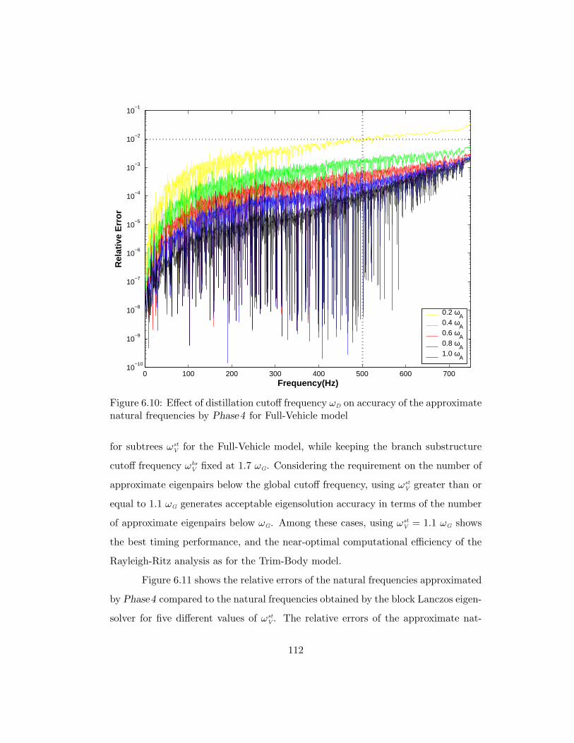
0 100 200 300 400 500 600 70010

−10

10−9

10−8

10−7

10−6

10−5

10−4

10−3

10−2

10−1

Frequency(Hz)

Rel

ativ

e E

rro

r

0.2 ωA

0.4 ωA

0.6 ωA

0.8 ωA

1.0 ωA

Figure 6.10: Effect of distillation cutoff frequency ωD on accuracy of the approximatenatural frequencies by Phase4 for Full-Vehicle model

for subtrees ωst

Vfor the Full-Vehicle model, while keeping the branch substructure

cutoff frequency ωbs

Vfixed at 1.7 ωG. Considering the requirement on the number of

approximate eigenpairs below the global cutoff frequency, using ωst

Vgreater than or

equal to 1.1 ωG generates acceptable eigensolution accuracy in terms of the number

of approximate eigenpairs below ωG. Among these cases, using ωst

V= 1.1 ωG shows

the best timing performance, and the near-optimal computational efficiency of the

Rayleigh-Ritz analysis as for the Trim-Body model.

Figure 6.11 shows the relative errors of the natural frequencies approximated

by Phase4 compared to the natural frequencies obtained by the block Lanczos eigen-

solver for five different values of ωst

V. The relative errors of the approximate nat-

112

Table 6.15: Effect of starting subspace cutoff frequency ωst


eigensolution accuracy and performance of Phase4 for Full-Vehicle model

ωst


ratio of V0 eigenpairs (%) timing(sec.) memory(MB)

1.0 8702 7334 84.2 3444 1189

1.1 9567 7418 77.5 3798 1472

1.2 10682 7431 69.5 4316 1775

1.3 11688 7435 63.6 4943 2118

1.4 12734 7438 58.4 5715 2508

0 100 200 300 400 500 600 70010

−10

10−9

10−8

10−7

10−6

10−5

10−4

10−3

10−2

10−1

Frequency(Hz)

Rel

ativ

e E

rro

r

1.0 ωG

1.1 ωG

1.2 ωG

1.3 ωG

1.4 ωG

Figure 6.11: Effect of starting subspace cutoff frequency ωst


accuracy of Phase4 for Full-Vehicle model

113

Table 6.16: Effect of starting subspace cutoff frequency ωbs


on the performance and eigensolution accuracy of Phase4 for Full-Vehicle model

ωbs


ratio of V0 eigenpairs (%) timing(sec.) memory(MB)

1.1 9180 7397 80.5 3486 1320

1.3 9357 7409 79.1 3618 1370

1.5 9533 7415 77.7 3728 1420

1.7 9567 7418 77.5 3798 1472

1.9 9867 7419 75.1 3878 1519

0 100 200 300 400 500 600 70010

−10

10−9

10−8

10−7

10−6

10−5

10−4

10−3

10−2

10−1

Frequency(Hz)

Rel

ativ

e E

rro

r

1.1 ωG

1.3 ωG

1.5 ωG

1.7 ωG

1.9 ωG

Figure 6.12: Effect of starting subspace cutoff frequency ωbs


on the accuracy of the natural frequencies computed by Phase4 for Full-Vehiclemodel

114

ural frequencies below 500 Hz are nearly indistinguishable for all the cases. The

maximum relative error of the approximate natural frequencies below the highest

excitation frequency, 500 Hz, is 0.001. Therefore, ωst

V= 1.1 ωG is chosen as a near-

optimal value for this model based on the eigensolution accuracy, the performance

measured by elapsed time and memory usage, and the computational efficiency of

the Rayleigh-Ritz analysis.

For branch substructures of this model, the effect of changing the starting

subspace cutoff frequency ωbs

Vfor branch substructures is shown in Table 6.16 and

Figure 6.12. Here, ωst

Vis fixed at 1.1 ωG. The starting subspace cutoff frequency

ωbs

Vfor branch substructures does not have as great an effect on the approximate

eigensolution accuracy and the performance of Phase4 as the starting subspace cut-

off frequency for subtrees ωst

V, as was observed for the Trim-Body model. As the

starting subspace cutoff frequency for branch substructures ωbs

Vincreases, the dimen-

sion of the starting subspace increases slightly, and the number of the approximate

eigenpairs below the global cutoff frequency increases slightly, as well. The relative

errors of the natural frequencies approximated by Phase4, although small, are most

visible in the frequency range between 500 Hz and 750 Hz as shown in Figure 6.12.

Considering the requirement on the number of approximate eigenpairs (7,413), the

cases for which ωbs

V≥ 1.5 ωG generate acceptable eigensolutions in terms of the

number of approximate eigenpairs below the global cutoff frequency. However, the

dimension of the starting subspace, along with the elapsed time, increases signifi-

cantly from ωbs

V= 1.7 ωG to ωbs

V= 1.9 ωG without any significant improvement in the

eigensolution accuracy. Therefore, we choose ωbs

V= 1.7 ωG as a near-optimal value

for this model.

115

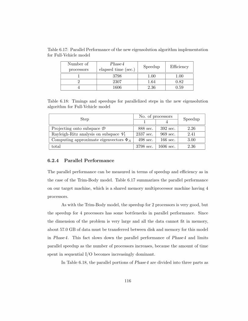
Table 6.17: Parallel Performance of the new eigensolution algorithm implementationfor Full-Vehicle model



1 3798 1.00 1.00

2 2307 1.64 0.82

4 1606 2.36 0.59

Table 6.18: Timings and speedups for parallelized steps in the new eigensolutionalgorithm for Full-Vehicle model


Speedup1 4

Projecting onto subspace D 888 sec. 392 sec. 2.26


Computing approximate eigenvectors ΦA 498 sec. 166 sec. 3.00

total 3798 sec. 1606 sec. 2.36

6.2.4 Parallel Performance

The parallel performance can be measured in terms of speedup and efficiency as in

the case of the Trim-Body model. Table 6.17 summarizes the parallel performance

on our target machine, which is a shared memory multiprocessor machine having 4

processors.

As with the Trim-Body model, the speedup for 2 processors is very good, but

the speedup for 4 processors has some bottlenecks in parallel performance. Since

the dimension of the problem is very large and all the data cannot fit in memory,

about 57.0 GB of data must be transferred between disk and memory for this model

in Phase4. This fact slows down the parallel performance of Phase4 and limits

parallel speedup as the number of processors increases, because the amount of time

spent in sequential I/O becomes increasingly dominant.

In Table 6.18, the parallel portions of Phase4 are divided into three parts as

116

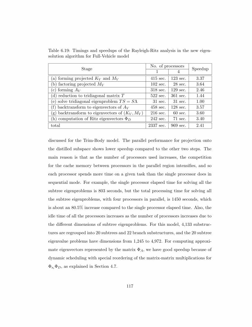
Table 6.19: Timings and speedups of the Rayleigh-Ritz analysis in the new eigen-solution algorithm for Full-Vehicle model

StageNo. of processors

Speedup1 4

(a) forming projected KV and MV 415 sec. 123 sec. 3.37



(d) reduction to tridiagonal matrix T 522 sec. 361 sec. 1.44

(e) solve tridiagonal eigenproblem TS = SΛ 31 sec. 31 sec. 1.00



(h) computation of Ritz eigenvectors ΦD 242 sec. 71 sec. 3.40

total 2337 sec. 969 sec. 2.41

discussed for the Trim-Body model. The parallel performance for projection onto

the distilled subspace shows lower speedup compared to the other two steps. The

main reason is that as the number of processors used increases, the competition

for the cache memory between processors in the parallel region intensifies, and so

each processor spends more time on a given task than the single processor does in

sequential mode. For example, the single processor elapsed time for solving all the

subtree eigenproblems is 803 seconds, but the total processing time for solving all

the subtree eigenproblems, with four processors in parallel, is 1450 seconds, which

is about an 80.5% increase compared to the single processor elapsed time. Also, the

idle time of all the processors increases as the number of processors increases due to

the different dimensions of subtree eigenproblems. For this model, 4,133 substruc-

tures are regrouped into 20 subtrees and 22 branch substructures, and the 20 subtree

eigenvalue problems have dimensions from 1,245 to 4,972. For computing approxi-

mate eigenvectors represented by the matrix ΦA, we have good speedup because of

dynamic scheduling with special reordering of the matrix-matrix multiplications for

ΦsiΦD, as explained in Section 4.7.

117

More detailed parallel performance results for the Rayleigh-Ritz analysis are

shown in Table 6.19. We have good speedups for steps (a), (b), (f), (g), and (h) as

shown in the table. Forming AV in step(c) shows low speedup due to the nature

of parallelizing solving a triangular system as for the Trim-Body model. However,

the bottleneck in parallel performance is the step for reduction of a dense matrix

to tridiagonal form, step (d), as we have seen for the Trim-Body model. We need

to improve the parallel performance of the tridiagonalization process of a full dense

matrix.

6.2.5 Overall Performance and Eigensolution Accuracy

The performance of Phase4 for the Full-Vehicle model is summarized in Table 6.20,

reflecting a cutoff frequency of 3,750 Hz for substructure eigenproblems, a global

cutoff frequency of 750 Hz, a distillation cutoff frequency of 2,250 Hz, a maximum

subtree size of 5,000, a starting subspace cutoff frequency for subtrees of 825 Hz,

and a starting subspace cutoff frequency for branch substructures of 1,275 Hz.

Table 6.20 summarizes the performance comparison between Phase4 and the

block Lanczos eigensolver on two different subspaces. In this table, the maximum

memory size in the Lanczos runs is set to 2.0 GB for the purpose of comparison

with Phase4because Phase4 uses less than 2.0 GB of memory. For the Lanczos

runs, the reciprocal eigenvalue problem was solved to exploit the diagonal stiffness

matrices KA and KD since this model does not have any rigid body modes caus-

ing the singularity of the stiffness matrices. This indicates that we can save the

very expensive reorthogonalization cost of Lanczos vectors by reorthogonalizing the

Lanczos vectors with respect to the diagonal stiffness matrices KA and KD instead

of reorthogonalizing them with respect to the block-sparse mass matrices MA and

MD. The subspace iteration (SI) method on the substructure eigenvector subspace

cannot complete the job to get an acceptable accuracy of the approximate eigenso-

118

Table 6.20: Performance comparison of Phase4 with the block Lanczos eigensolveron two different subspaces for Full-Vehicle model

Performance Phase4 Lanczos on D Lanczos on A

Elapsed time 0:26:47 4:26:20 9:22:25

System time 0:02:51 1:24:48 2:54:49

Memory usage (MB) 1913.5 2000.0 2000.0

Disk usage (GB) 14.1 11.9 19.8

Data transfer (GB) 55.7 2493.2 5058.7

No. of eigenpairs 7418 7447 7451

0 100 200 300 400 500 600 700 75010

−10

10−8

10−6

10−4

10−3

10−2

10−1

Frequency (Hz)

Rel

ativ

e E

rro

r

Phase4

Lanczos on D

Figure 6.13: Accuracy of the natural frequencies computed by Phase4 and the blockLanczos eigensolver on the distilled subspace (D) for Full-Vehicle model

119

lution because the final Rayleigh-Ritz analysis requires more than 8.0 GB memory,

which is the maximum memory space available for our target machine.

Apparently, Phase4 outperforms the Lanczos eigensolver for the reduced

eigenvalue problem on the two different subspaces in terms of the elapsed time and

data transfer with a small sacrifice in eigensolution accuracy. Phase4 is about 10

times faster than the Lanczos eigensolver on the distilled subspace D and is about 21

times faster than the Lanczos eigensolver on the substructure eigenvector subspace

A . Since a significant amount of I/O is required during the Lanczos iterations in the

block Lanczos eigensolver, the system time of the block Lanczos runs on the subspace

A is 30.9% of the total elapsed time. By contrast, the system time in Phase4 is only

11.1% of the total elapsed time, which is less than 3 minutes. The block Lanczos

eigensolver on the subspace A uses 19.8 GB of disk space, and, significantly, transfers

more than 5.0 terabytes of data. Compared to the block Lanczos performance on

the subspace A , Phase4 transfers only 55.7 GB of data using 14.1 GB of disk space.

Figure 6.13 shows the relative errors of the approximate natural frequencies

computed by Phase4 compared to the natural frequencies computed by the block

Lanczos eigensolver on the substructure eigenvector subspace. Every approximate

natural frequency computed by Phase4 has a relative error less than 0.35e−2 even

though 33 fewer modes are found than the actual number of eigenpairs on the sub-

structure eigenvector subspace, according to the inertia of the matrix (KA−ωG

2MA).

Note that Phase4 computes 4,034 approximate eigenpairs below the highest exci-

tation frequency of 500 Hz, which is only three fewer than the actual number of

natural frequencies.

The distilled subspace for the block Lanczos run on the distilled subspace

is formed by using the maximum subtree size of 5,000 and the distillation cut-

off frequency of 3,000 Hz. The maximum relative error of the natural frequencies

approximated on the distilled subspace compared to the natural frequencies approx-

120

0 150 300 450 600 7500

0.1

0.3

0.5

0.7

0.9

1

Frequency (Hz)

Co

sin

e o

f th

e p

rin

cip

al a

ng

les

Figure 6.14: Cosine of the principal angles between two eigenspaces computed byPhase4 and the block Lanczos eigensolver on the subspace A for Full-Vehicle model

imated on the substructure eigenvector subspace by the block Lanczos eigensolver

is 0.75e−3. This indicates that the distillation process produces a reduced subspace

(31,698 reduced from 68,521) containing almost all the eigenpairs below the global

cutoff frequency of 750 Hz. Only one fewer natural frequency below the highest

excitation frequency of 500 Hz is found as a result of the distillation process.

We can verify the accuracy of the eigenvectors approximated by Phase4 by

computing the singular values of ΦTLMAΦA to obtain the principal angles between

the two eigenspaces as explained for the Trim-Body model. Figure 6.14 shows the

cosines of the principal angles between the two eigenspaces computed by Phase4 and

the block Lanczos eigensolver. Closeness of cosines of the principal angles to unity

indicates the two eigenspaces represented by ΦA and ΦL are very close together.

121

Therefore, a very good approximate eigenspace for modal frequency response anal-

ysis is obtained by the new eigensolution algorithm.

6.3 8.4M DOF Model

The last model is another full vehicle model that has 8.4 million FE degrees of

freedom. This model is a typical model for which we are aiming to compute the

eigensolution for modal frequency response analysis. We will refer to this model

as the “8.4M DOF” model. The block Lanczos eigensolver of MSC.Nastran cannot

solve the eigenproblem of this model on the FE discretization subspace because of

its size. Even the eigenproblem on the substructure eigenvector subspace (A) of

order 135, 924 cannot be solved by the block Lanczos eigensolver of MSC.Nastran

because of the 8 GB memory constraint of the machine. Hence, the completion of

the AMLS run for this model using the new eigensolution algorithm demonstrates

that the new eigensolution algorithm extends the capability of solving eigenproblems

for large structural systems with high modal density on our target machine. For

this model we are not optimizing parameters as with the other two models. Instead,

we use the default parameter values from the Full-Vehicle model.

For the 8.4M DOF model, the frequency range of interest is from zero to

500 Hz for modal frequency response analysis. The highest excitation frequency

ωF is 2π·(500 Hz). The global eigenproblem cutoff frequency ωG is 1.5 ωF. A cutoff

frequency for substructure eigenproblems ωA is 5.0 ωG, a distillation cutoff frequency

ωD is 0.6 ωA, a starting subspace cutoff frequency for subtrees ωst

Vis 1.1 ωG, a starting

subspace cutoff frequency for branch substructures ωbs

Vis 1.7 ωG, and a maximum

subtree size is 5,000. The number of output degrees of freedom requested by the user

is 245, and the number of forced degrees of freedom is 7. This model has no rigid

body modes, but 7 low frequency modes with natural frequencies below 5.25 Hz.

Phase2 of the AMLS software automatically divides this FE model into

122

Table 6.21: Overall performance of the AMLS software for 8.4M DOF model

PhaseElapsed time Memory usage Data transfer Disk usage(hh:mm:ss) (GB) (GB) (GB)

Phase2 00:34:58 2.270 11.7 14.5

Phase3 03:32:53 3.921 238.9 93.8

Phase4 01:36:08 3.944 286.2 46.8

Phase5 00:25:39 3.104 106.4 17.2

18,373 substructures on 31 levels. The substructure size ranges up to 2,190 degrees

of freedom. For the given substructure eigenproblem cutoff frequency ωA, Phase3

computes 135,924 substructure eigenvectors and projects the system matrices K

and M onto this substructure eigenvector subspace. Phase4 solves the reduced

eigenproblem of order 135,924, looking for more than 11,000 eigenpairs. Since the

number of output FE degrees of freedom requested by the user for this model is only

245, the time spent in Phase5, which computes only these entries in the approximate

eigenvectors on the FE subspace, is not as great as the time spent in other phases.

Table 6.21 shows the overall performance of the AMLS software. Here, four

processors are used during the execution of each phase. For this large model with

high modal density, the elapsed time for Phase3 is greater than for all of the other

phases combined. Phase3 uses the largest amount of disk space among the phases to

save memory usage. Each phase uses a maximum memory space of less than 4.0 GB.

Note that Phase4 is designed to use the maximum memory space needed for solving

the Rayleigh-Ritz eigenproblem because memory usage in Phase4 usually reaches

the maximum during solving Rayleigh-Ritz eigenproblem for those models having

high modal density.

Since we cannot solve the reduced eigenproblem on the substructure eigenvec-

tor subspace by the block Lanczos eigensolver, we cannot obtain numerical results on

the substructure eigenvector subspace to compare with those computed by Phase4.

To get eigensolution results for an accuracy comparison with Phase4 we run the

123

Table 6.22: Performance comparison between Phase4 and the block Lanczos eigen-solver on the distilled subspace for 8.4M DOF model

Performance Phase4 Lanczos on D

Elapsed time (hh:mm:ss) 01:36:08 26:16:06

System time (hh:mm:ss) 00:15:54 05:42:42

User time (hh:mm:ss) 04:25:20 74:06:21

Memory usage (GB) 3.9 4.0

Disk usage (GB) 46.8 25.3

Data transfer (GB) 286.2 9443.9

block Lanczos eigensolver on the distilled subspace obtained with a maximum sub-

tree size of 5,000 and a distillation cutoff frequency of 0.6 ωG. The performance and

eigensolution accuracy of the Phase4 results are compared with the results from the

block Lanczos solver on the distilled subspace in the following subsections. Also,

the parallel performance of Phase4 is investigated in the last subsection.

6.3.1 Phase4 Performance

The performance of Phase4 compared to the block Lanczos eigensolver on the dis-

tilled subspace is summarized in Table 6.22. For this run, Phase4 approximates

11,027 eigenpairs below the global cutoff frequency and the Lanczos eigensolver on

the distilled subspace approximates 11,073 eigenpairs below ωG

2. Phase4 obtains

over 99.5% of the actual number of eigenpairs below the global cutoff frequency

on the distilled subspace, and shows excellent timing performance compared to the

block Lanczos eigensolver on the distilled subspace. The results of the block Lanc-

zos eigensolver were obtained by solving the reciprocal eigenvalue problem as for

the Full-Vehicle model.

Table 6.22 shows the performance comparison between Phase4 and the block

Lanczos eigensolver on the distilled subspace. The maximum memory size for the

block Lanczos eigensolver was set as 4.0 gigabytes for comparison with Phase4. The

124

block Lanczos eigensolver performed 54 factorizations, 53 Lanczos runs, and 3,320

Lanczos iterations with a blocksize of 7. Phase4 is 16.4 times faster than the block

Lanczos eigensolver even on the distilled subspace of dimension 57,188. With a

similar maximum memory usage, the block Lanczos eigensolver uses 21.5 GB less

disk space than Phase4 uses, but requires more than 9.4 terabytes of data transfer,

which is 33 times as much data transfer as the amount of data transfer required by

Phase4.

6.3.2 Eigensolution Accuracy of Phase4

The accuracy of the approximate natural frequencies computed by Phase4 is mea-

sured by computing the relative errors of the natural frequencies compared to the

natural frequencies computed by the block Lanczos eigensolver on the distilled sub-

space.

As shown in Figure 6.15, the maximum relative error of approximate natural

frequencies compared to those obtained by the block Lanczos eigensolver is 0.27e−2

over the frequency range from zero to 750 Hz. Compared to the actual number of

eigenpairs (11,073) on the distilled subspace, according to the inertia of the matrix

(KD − ωG

2MD), 46 fewer global modes are found by Phase4. Below the highest

excitation frequency 500 Hz, the number of approximate natural frequencies com-

puted by Phase4 is 6,112 and the number of natural frequencies obtained by the

block Lanczos eigensolver on the distilled subspace is 6,114. Also, the maximum

relative error of approximate natural frequencies below 500 Hz is less than 0.34e−3.

Therefore, we can conclude that a good approximate eigensolution below the high-

est excitation frequency of 500 Hz is obtained by the new eigensolution algorithm,

along with excellent timing performance.

125

0 100 200 300 400 500 600 700 75010

−10

10−8

10−6

10−4

10−3

10−2

10−1

Frequency (Hz)

Rel

ativ

e E

rro

r

Figure 6.15: Accuracy of the approximate natural frequencies computed by Phase4

compared to the natural frequencies approximated by the block Lanczos eigensolveron the distilled subspace for 8.4M DOF model.

6.3.3 Parallel Performance of Phase4

As for the Full-Vehicle model, the parallel performance results of Phase4 for the

8.4M DOF model are generated on our target machine having 4 processors. The

overall parallel performance of Phase4 is shown in Table 6.23. The speedups and

efficiencies with 2 and 4 processors are similar to those for the Full-Vehicle model.

Table 6.24 summarizes the parallel performance of the new eigensolution

algorithm in detail. As discussed for the previous two models, the parallel perfor-

mance of projecting the eigenproblem onto the distilled subspace D is affected by

more multiple processor idle times due to the I/O requested by multiple processors

and the different dimensions of subtree eigenproblems. We have good speedup for

126

Table 6.23: Parallel Performance of the new eigensolution algorithm for 8.4M DOFmodel



1 14274 1.00 1.00

2 8706 1.63 0.81

4 5766 2.47 0.61

Table 6.24: Timings and speedups of Rayleigh-Ritz analysis in the new eigensolutionalgorithm for 8.4M DOF model


Speedup1 4

Projecting onto subspace D 1919 sec. 790 sec. 2.42


(a) forming projected KV and MV 2859 sec. 875 sec. 3.26



(d) reduction to tridiagonal matrix T 2188 sec. 1479 sec. 1.47

(e) solving tridiagonal eigenproblem TS = SΛ 84 sec. 84 sec. 1.00



(h) computing Ritz eigenvectors ΦD 1263 sec. 398 sec. 3.17

Computing approximate eigenvectors ΦA 1304 sec. 445 sec. 2.93

total 14274 sec. 5766 sec. 2.47

computing approximate eigenvectors represented by ΦA even though each processor

have to wait until more than 1.4 GB of eigenvector data is written to the disk by a

single processor.

The detailed performance results for Rayleigh-Ritz analysis are summarized

in Table 6.24. Speedups for all the steps in the Rayleigh-Ritz analysis are similar to

those for the Full-Vehicle model. The bottleneck of parallel performance is reduction

of the full matrix AV to a tridiagonal form as we observed for the previous two

models. The computational routine for tridiagonal reduction should be improved by

127

using different parallelism for shared memory multiprocessor machines, as discussed

in [65].

6.4 Summary of Numerical Results

In this chapter, numerical results for three practical FE models from automotive

industry have been presented. For the first two models, the sensitivity of four pa-

rameter values on the performance and accuracy of the approximate eigensolution

algorithm was investigated. We observed that the most sensitive parameter on tim-

ing performance is the maximum subtree size and the most sensitive parameter on

eigensolution accuracy is the distillation cutoff frequency ωD. The starting subspace

cutoff frequencies, ωst

Vand ωbs

V, are less sensitive than those two parameters.

The parallel performance of Phase4 is demonstrated for three models. Over-

all speedup and efficiency of Phase4 for three models are about 2.4 and 60%, re-

spectively, when 4 processors are used. However, we can improve the parallel perfor-

mance of Phase4 by resolving the parallel performance bottlenecks in the algorithm.

Householder reduction to tridiagonal form in Rayleigh-Ritz analysis is a significant

parallel performance bottleneck, and its parallel implementation must be revised for

performance improvement.

For the Trim-Body model, Phase4 computes all the natural frequencies

(2,381) below the highest excitation frequency 400 Hz with the relative error less

than 0.34e−3 compared to the natural frequencies computed by the block Lanczos

eigensolver. By computing the principal angles between two eigenspaces computed

by Phase4 and the block Lanczos solver, we verify the good quality of the eigenspace

computed by Phase4. The new eigensolution algorithm solves the reduced eigen-

problem in less than 15 minutes, and uses about 2.0 GB of memory space and

10.0 GB of disk space. Through the distillation process, we achieve 40% dimen-

sional reduction of the reduced eigenproblem from 45,122 to 26,965 without losing

128

much accuracy.

For the Full-Vehicle model, which has more substructure eigenvectors below

the cutoff (68,521) than the Trim-Body model, Phase4 computes only three fewer

eigenpairs than the number of actual eigenpairs below 500 Hz (4037). The relative

errors of the approximate natural frequencies below 500 Hz are less than 0.001

compared to those obtained by the block Lanczos eigensolver. Phase4 solves the

reduced eigenproblem in less than 30 minutes, using less than 2.0 GB of memory

space and 15.0 GB of disk space. The good quality of the eigenspace computed

by Phase4 was demonstrated by computing the principal angles between the two

eigenspaces computed by Phase4 and the block Lanczos eigensolver. By means of

the distillation process, 54% dimensional reduction of the reduced eigenproblem has

been done within 0.75e−3 relative error of approximate natural frequencies.

Finally, the new eigensolution algorithm was tested for an 8.4M DOF model,

which is a typical FE model that we are aiming to solve for many eigenpairs. The

block Lanczos eigensolver in the commercial software MSC.Nastran cannot solve

this problem on our target machine due to the size of the problem (135,924 ×135,924). However, Phase4 solves this problem within 2 hours with good accuracy,

using 4.0 GB of memory space and 50.0 GB of disk space. Using the same global

and distillation cutoff frequencies used for the Full-Vehicle model, 62% dimensional

reduction of the reduced eigenproblem has been done through the distillation pro-

cess. Therefore, the numerical results for this model demonstrates that the new

eigensolution algorithm and its implementation present capabilities for solving large

eigenproblems with many eigenpairs.

129

Chapter 7

Conclusions and Future Work

7.1 Conclusions

In this dissertation, a new eigensolution algorithm for the reduced eigenproblem

produced by the AMLS transformation is presented for large structural systems

with many eigenpairs. The new eigensolver in combination with AMLS is advanta-

geous for solving huge FE models with many eigenpairs because it takes much less

computer time and resource than the state-of-the-art eigensolver while maintaining

acceptable eigensolution accuracy. To verify the efficiency of the new eigensolution

algorithm, a sequential version of the new eigensolution algorithm has been imple-

mented and optimized. A parallel implementation with OpenMP API for shared

memory multiprocessor machines has been completed for performance improvement.

In Chapter 4, using the properties of the stiffness and mass matrices KA and

MA from the AMLS transformation, a new distilled subspace of the substructure

eigenvector subspace is built by defining subtrees, solving subtree eigenproblems,

and truncating subtree and branch substructure eigenspaces. The reduced eigen-

problem is then projected onto this distilled subspace, utilizing the sparsity of the

system matrices KA and MA. Using a good initial guess of a starting subspace on

130

the distilled subspace, which is represented by a very sparse matrix, one subspace

iteration recovers as much accuracy as needed for approximation. Hence, the di-

mension of the Ritz subspace for Rayleigh-Ritz analysis is minimized and the Ritz

subspace is represented by a sparse matrix. Approximate global eigenvalues can be

computed by solving the Rayleigh-Ritz eigenproblem, and the corresponding global

eigenvectors are recovered by inexpensive matrix-matrix multiplications. In addi-

tion, remedies for a nearly singular stiffness matrix and an indefinite mass matrix are

presented for robustness of the implementation of the new eigensolution algorithm.

In Chapter 5, a parallel algorithm of the new eigensolution method is pro-

posed using the OpenMP API for shared memory multiprocessor machines. Op-

portunities for parallelization of each step in the new eigensolution algorithm are

carefully investigated and exploited. Due to the nature of substructuring, projecting

the reduced eigenproblem onto the distilled subspace and computing approximate

eigenvectors on the substructure eigenvector subspace can be done simultaneously

by subtrees and branch substructures without any communication among the pro-

cessors. For the steps of projecting the eigenproblem onto Ritz subspace V1 and

computing Ritz eigenvectors ΦD in the Rayleigh-Ritz analysis, the operations for

those steps can be done individually and simultaneously by subtrees and branch

substructures with very few communication cost. The parallelism for the eigen-

problem for Ritz values is different from the rest of the algorithm. It involves a

more fine-grain type of parallelism, which denotes a refined parallelism on a lower

loop level.

In Chapter 6, numerical results for three practical FE models from automo-

tive industry are presented to demonstrate the performance and accuracy of the

new eigensolution algorithm compared to those of the block Lanczos algorithm. For

the Trim-Body model, the new eigensolution algorithm computes all the natural

frequencies (2,381) below the highest excitation frequency 400 Hz, maintaining the

131

relative error of the natural frequencies less than 0.34e−3. The new eigensolution al-

gorithm in combination with AMLS solves the FE eigenproblem of this model in less

than 50 minutes, using about 2.5 GB of memory space and 25.0 GB of disk space.

Compared to the previous algorithm [1] for the reduced eigenproblem of this model,

the new eigensolution algorithm solves this eigenproblem with much less computer

time with improved eigensolution accuracy in terms of relative errors of the natural

frequencies. For the Full-Vehicle model, Phase4 computes 4034 eigenpairs that is

only three fewer than the actual number of eigenpairs below 500 Hz. The maximum

relative error of the natural frequencies below 500 Hz is less than 0.001. The new

eigensolution algorithm in combination with AMLS solves this FE eigenproblem of

this model within 2 hours, using about 2.2 GB of memory space and 35.0 GB of disk

space. Finally, the new eigensolution algorithm was investigated for a very modally

dense model having more than 11,000 eigenpairs below the global eigenproblem cut-

off frequency 750 Hz. Any existing eigensolver software cannot solve this problem

on our target machine due to the excessive dimension and high modal density of

this problem. However, the new eigensolver in conjunction with AMLS solves this

problem within 7 hours with good accuracy, using about 4.0 GB of memory space

and 94.0 GB of disk space. This demonstrates that the new eigensolution algorithm

and its implementation in combination with the AMLS software presents capabili-

ties for solving for many eigenpairs of large eigenproblems. Due to the significant

improvement in the eigensolution algorithm for the reduced problem, the dominant

term in the cost of the AMLS software for modally dense models is shifted from

solving the reduced eigenproblem to the AMLS transformation.

In the appendix, a new method for solving the augmented eigenproblem for

residual flexibility is developed to mitigate the loss of accuracy in modal frequency

response analysis at very little additional computational cost. This new method

can achieve a significant performance improvement for the models having many

132

static vectors compared to the algorithm implemented in the proprietary software

MSC.Nastran.

7.2 Future Work

As we discussed in Chapter 6, the parallelism of the tridiagonal reduction algorithm

should be revised to improve the parallel performance of Phase4. Since this rou-

tine takes typically about one fourth of the total elapsed time of Phase4, a large

performance gain is expected by improving the parallel performance of this tridi-

agonalization algorithm. The other parallel algorithms for tridiagonal reduction as

discussed in [68, 73] might be adopted for efficient parallelization of the tridiagonal

reduction for shared memory multiprocessor machines.

In solving subtree eigenproblems, a dense eigensolver is used because more

than 40% of the full eigenpairs are needed for subtree eigenproblems. However,

a robust shift-invert block Lanczos eigensolver might be faster than Householder

eigensolution algorithm for subtree eigenproblems. If a robust non-proprietary block

Lanczos eigensolver becomes available in the public domain, the shift-invert block

Lanczos eigensolver can be used for solving subtree eigenproblems utilizing sparsity

of the system matrices.

The AMLS software including this new eigensolution algorithm has been a

commercial application in automotive industry. The current implementation was

targeted for microprocessor-based workstations with shared memory multiproces-

sors. For this reason, the parallel implementation has been done with the OpenMP

Application Programming Interface (API) for shared memory multiprocessor ma-

chines. Since the automotive industry requires more aggressive parallelism for dis-

tributed memory multiprocessor machines, like Linux clusters, MPI (Message Pass-

ing Interface) parallelization should be started to satisfy the near future demand

of the automotive industry. The parallelism for distributed memory multiproces-

133

sors might be quite different from the current implementation for shared memory

multiprocessors. More sophisticated parallelism is required for massively parallel

implementation of the new eigensolution algorithm for distributed memory multi-

processors. For example, the coarse-grain type of parallel algorithm for projection

of the reduced eigenproblem onto the distilled subspace should be modified, so that

the computation of subtree eigenproblems can be distributed to as many processors

as possible to achieve good speedup and efficiency of parallelism. Currently, the

MPI parallelization of the AMLS transformation (Phase3) is in process [2].

7.3 Final Remarks

The new eigensolution algorithm has some limitations as other eigensolution al-

gorithms. How large a FE model can be handled by AMLS is dependant on the

sparsity of FE matrices as well as the size of the FE model. For a very large FE

model with high matrix density in the system matrices, Phase3 of AMLS requires

significant amount of computer time and resource to transform the model. For

modally dense models with high global cutoff frequency, the number of substructure

eigenvectors kept by Phase3 is very large. For these models, the required number

of global eigenpairs determines the dimension of Rayleigh-Ritz analysis in the new

eigensolution algorithm used in Phase4. The eigenproblems for these models can be

solved if the physical memory space is large enough for the Rayleigh-Ritz analysis

because Phase4 is designed to use the maximum memory space required for the

Rayleigh-Ritz analysis.

This new eigensolution algorithm has been implemented within the AMLS

software and released commercially since 2002. Since then, almost every automo-

tive company has been using the AMLS software for NVH (Noise, Vibration, and

Harshness) analysis due to the benefits of shortened job turn-around time in the so-

lution process with acceptable eigensolution accuracy. For the past couple of years

134

the performance and acceptable accuracy of this new eigensolution algorithm has

been approved by the automotive industry. Due to AMLS, the automotive industry

can increase model size for high frequency resolution, while maintaining adequate

solution turn-around time within design process times. This capability of AMLS

offers great commercial advantages to automotive manufactures. Therefore, the im-

pact of AMLS can be continuously widespread over the broad range of engineering

applications.

135

Appendix A

Augmented Eigenproblem for

Residual Flexibility

When the mode superposition method is used to approximate modal frequency

response, the structural response of a FE model is not quite accurate due to the

truncation of higher frequency modes. The contribution to the structural response

from truncated high frequency modes is approximately compensated by adding static

responses into the modal subspace spanned by the global eigenvectors kept [41,

48, 76]. Here, a static response is defined as a static deflection of the structure

which results when a unit force is exerted on one forced degree of freedom, while

the remaining degrees of freedom are force free [41]. A previous implementation

[1] of adding static responses to the modal subspace spanned by the approximate

eigenvectors was quite costly since the dimension of the eigenvalue problem to be

solved for orthonormal static responses (or static vectors) was the sum of the number

of the global eigenvectors kept and the number of force vectors for a FE model.

By doing more precise modified block Gram-Schmidt orthogonalization for

static vectors against the approximate global eigenvectors kept from solving the

reduced eigenproblem produced by AMLS, the numerical orthogonality condition

136

between the approximate global eigenvectors kept and the static vectors is well

established. So, the precise orthogonality between the approximate global eigen-

vectors and the static vectors eventually induces a smaller eigenvalue problem for

orthonormal static vectors than the eigenproblem produced by the previous algo-

rithm of Kaplan [1]. The relationship between residual flexibility technique and

block orthogonalization procedure of static vectors is explained in the first subsec-

tion. The new algorithm for computing residual flexibility eigensolution is then

summarized, followed by the detailed explanation of the new algorithm in the later

two subsections.

A.1 Residual Flexibility and Block Orthogonalization

An approximation of the responses for the truncated eigenvectors [41] can be ex-

pressed as

XR = (Φt Λ−1t ΦT

t ) FA (A.1)

where Λt is a diagonal matrix containing truncated eigenvalues, Φt is a matrix

containing the corresponding truncated eigenvectors in columns, and FA is a matrix

containing force vectors in columns. The coefficient matrix of FA in Equation (A.1)

is defined as residual flexibility matrix, which is given by

Gt = Φt Λ−1t ΦT

t . (A.2)

Since the residual flexibility matrix is unknown, the same value can be obtained

through the knowledge of the elastic flexibility matrix and the eigenpairs kept for

the system as:

Gt = Ge − ΦkΛ−1k ΦT

k , (A.3)

where

Ge = ΦeΛ−1e ΦT

e = K−1A

137

is the elastic flexibility matrix, Λk is a diagonal matrix containing kept eigenvalues,

Φk is a matrix containing the corresponding kept eigenvectors in columns, and Φe is

a matrix containing orthonormal elastic (or flexible) modes. Thus, the response for

the truncated eigenvectors, which can be called as the residual flexibility vectors,

represented by the matrix XR, can be expressed by another form

XR = ( K−1A − Φk Λ−1

k ΦTk ) FA. (A.4)

The Equation (A.4) can be rewritten as

XR = [ I − Φk Λ−1k ΦT

k KA ] (K−1A FA)

= [ I − Φk Λ−1k ΦT

k KA ] XS (A.5)

where XS = (K−1A FA) is a matrix containing static vectors in columns, and [ I −

Φk Λ−1k ΦT

k KA ] can be viewed as an operator orthogonalizing XS against Φk with

respect to KA. Equation (A.5) implies that XR is a matrix containing in columns or-

thonormal static vectors against Φk with respect to KA. In other words, computing

residual flexibility vectors is equivalent to computing KA-orthonormal static vectors

against the kept global eigenvectors. Therefore, we can add the residual flexibility

vectors, which can be obtained by orthonormalizing static vectors against the kept

eigenvectors Φk with respect to the stiffness matrix KA, to the modal subspace.

A.2 Preliminary Residual Flexibility Eigensolution Al-

gorithm

After we obtain the approximate global eigenvectors below the global cutoff fre-

quency, we need to add static vectors to the modal subspace spanned by the global

eigenvectors as follows:

TR =[

Φk XS

]

. (A.6)

138

begin

1 Compute static vectors : XS = K−1A FA

2 Compute Ufor i = 1, 2, 3 do

3 Orthogonalize static vectors against Φk w.r.t. KA :XR ← [ I − ΦkUΦT

k KA ] XS

for j = 1, 2 do

4 Orthogonalize XR among themselves w.r.t. KA

end

if reorthogonalization is not needed then exitend

5 Project system matrices onto the subspace represented by XR :KX = XT

R KA XR, MX = XTR MA XR

6 Solve the small projected eigenproblem :KX QX = MX QX ΛX

7 Backtransform eigenvectors to eigenvectors on the subspace A :ΦR = XR QX , ΛR = ΛX

8 Add orthonormalized residual flexibility vectors to the modalsubspace :

Φm =[

Φk | ΦR

]

, Λm =

[

Λk 00 ΛR

]

end

Figure A.1: New augmented eigensolution algorithm for residual flexibilityeigensolution

The question of linear dependence of augmented subspace TR, however, arises be-

tween the global eigenvectors kept and the static vectors, and possibly between

static vectors themselves. In order to avoid linear dependence in the augmented

subspace, we have to orthogonalize static vectors against Φk and among themselves

with respect to KA.

The new algorithm to compute residual flexibility eigenpairs is shown in

Figure A.1. Here, we compute residual flexibility eigenvectors on the substructure

eigenvector subspace, instead of those on the FE subspace. After solving the reduced

eigenproblem on the substructure eigenvector subspace, the residual flexibility eigen-

pairs are computed on the same subspace using the AMLS transformed force vectors

139

represented by FA. In the following sections, the detailed explanation of the new

algorithm for computing the residual flexibility eigensolution is presented.

A.3 Block Orthogonalization Procedure

The matrix XS containing static vectors is defined by

XS = K−1A ( T T

A F )

= K−1A FA (A.7)

where F is a matrix containing force vectors in columns on the FE discretization

subspace, FA is a matrix containing force vectors in columns on the substructure

eigenvector subspace, and TA is the AMLS transformation matrix. Using the block

modified Gram-Schmidt algorithm (bMGS) by Bjorck [36], static vectors are orthog-

onalized against Φk with respect to KA by blocks as

XR ←nb∏

j=1

(

I − Φkj Uj ΦkTj KA

)

XS (A.8)

where Φk have been partitioned into nb column blocks, so Φkj is the jth column

block of the matrix Φk. The matrix Uj is an upper triangular matrix associated

with Φkj . The Equation (A.8) can be reformulated as another form:

XR ←nb∏

j=1

(

XSj − Φkj αj

)

(A.9)

where

αj = Uj ΦkTj KA XSj , (A.10)

and XSj is the static vectors orthonormalized against the eigenvectors represented

by (Φk)1:j−1. For the block modified Gram-Schmidt orthogonalization, the matrix

Uj is used instead of ΛA−1j in the classical Gram-Schmidt orthogonalization. If

the maximum value of αj for j (= 1, 2, · · · , nb) is less than some tolerance, then

140

Uj(1, 1) = λ−1l+1

for i = 2, 3, . . . , p do

1 Uj(1 : i−1, i) = −Uj(1:i−1, 1:i−1) Φk(: , l+1:l+i−1)T Keφl+iλ−1l+i

Uj(i, i) = λ−1l+i

end

Figure A.2: Algorithm for computing U in the block modified Gram-Schmidtorthogonalization

1 Y ( : , 1 : p−1) = Ke Φk( : , l+1 : l+p−1) diag(λ−1(l+1:l+p−1))

2 W (2 : p, 2 : p) = Φk( : , l+1 : l+p−1)T Y ( : , 1 : p−1)Uj(1, 1) = λ−1

l+1

for i = 2, 3, . . . , p do

3 Uj(1 : i−1, i) = −Uj(1 : i−1, 1 : i−1) W (2 : i, i)Uj(i,i) = λ−1

l+i

end

Figure A.3: More efficient algorithm for computing U in the block modifiedGram-Schmidt orthogonalization

the reorthogonalization process is terminated because the maximum value of αj

indicates the numerical orthogonality between Φkj and XSj with respect to KA.

The matrix Uj is computed before orthogonalization process for a block of

eigenvectors Φkj . The matrix U is defined by the recursion formulation [36] as shown

in Figure A.2. In Figure A.2, l is the number of previous eigenvectors ((j−1)p) before

Φkj , and p is the number of eigenvectors in each column block of Φk. The matrix

Uj(1 : i−1, i) represents the row elements from 1 to i−1 of the ith column vector in

the matrix Uj , and Y (:, 1 : p−1) represents the column vectors from 1 to p−1 in the

matrix Y . The number of eigenvectors in a block is typically set to 100 by numerical

experience for the optimal performance and accuracy of the block orthogonalization.

The computation for forming Uj requires matrix-vector operations, which is

inefficient in memory reuse for hierarchical memory system. By simple modification,

the algorithm can be improved so that it uses more matrix-matrix operations, which

are more efficient in memory reuse, instead of matrix-vector operations. Therefore,

141

the algorithm in Figure A.2 can be modified to do more matrix-matrix operations

as proposed in Figure A.3. In Figure A.3, Y is a rectangular matrix and W is an

upper triangular matrix for temporary use. Step 1 in Figure A.2 can be carefully

divided into three steps as shown in Figure A.3. Step 2 in Figure A.3 becomes a

matrix-matrix multiplication instead of matrix-vector multiplications in step 1 in

Figure A.2.

After calculation of Uj for each block, reorthogonalization process is pro-

ceeded until the coefficient matrix αj of Φkj , after the block modified Gram-Schmidt

orthogonalization, becomes less than the tolerance 10−9. However, the maximum

number of iteration is set to three for accuracy even though the twice Gram-Schmidt

orthogonalization is usually enough [40].

After KA-orthogonalization of the static vectors against Φk, the orthogonal-

ization among themselves is needed. Usually the number of static vectors is much

smaller than the number of global eigenvectors kept and significantly smaller than

their dimension. Unblocked modified Gram-Schmidt algorithm is used for orthog-

onalization among the static vectors themselves with respect to KA. To avoid the

linear dependence among the static vectors, the static vectors whose Euclidean norm

after orthogonalization is significantly smaller than the norm before orthogonaliza-

tion are eliminated.

A.4 Small Eigenproblem for Residual Flexibility

After the orthonormalized static vectors are computed, the stiffness and mass ma-

trices are projected onto the augmented subspace spanned by

TR = [ Φk XR ]. (A.11)

142

The stiffness matrix becomes

KR = T TR KA TR =

ΦTk KA Φk ΦT

k KA XR

(sym.) XTR KA XR

(A.12)

Similarly, the mass matrix becomes

MR = T TR MA TR =

ΦTk MA Φk ΦT

k MA XR

(sym.) XTR MA XR

(A.13)

Thanks to the orthogonality of Φk with respect to KA, the upper left block

diagonal submatrices in KR and MR become diagonal as ΦTk KA Φk = Λk and

ΦTk MAΦk = Ik. Moreover, the off-diagonal blocks of the two matrices, ΦT

k KAXR and

ΦTk MA XR become null matrices. The following derivations, using Equation (A.5)

and orthogonality condition of Φk with respect to KA and MA, explain the reason

of the cancellation.

ΦTk KA XR = ΦT

k KA XS − (ΦTk KA Φk ) Λ−1

k (ΦTk KA) XS

= ΦTk KA XS − (Λk Λ−1

k ) ΦTk KA XS

= 0

(A.14)

ΦTk MA XR = ΦT

k MA XS − (ΦTk MA Φk ) Λ−1

k (ΦTk KA) XS

= ΦTk MA XS − Ik Λ−1

k (Λk ΦTk MA) XS

= 0

(A.15)

Because of these cancellations, the system matrices projected onto the aug-

mented subspace spanned by TR can be expressed by

KR =

Λk 0

0 KX

=

Λk 0

0 XTR KA XR

(A.16)

and

MR =

I 0

0 MX

=

I 0

0 XTR MA XR

(A.17)

143

This leads to the small eigenvalue problem for residual flexibility eigenpairs

KX QX = MX QX ΛX , (A.18)

where ΛX ∈ Rnx×nx is a diagonal matrix containing residual flexibility eigenvalues,

QX ∈ Rnx×nx is a matrix containing the corresponding eigenvectors in its columns,

and nx is the number of the orthonormal residual flexibility eigenpairs. Therefore,

MA-orthonormalized residual flexibility eigenvectors and their corresponding eigen-

values are recovered as following.

ΦR = XR QX , ΛR = ΛX (A.19)

Finally, the residual flexibility eigenvectors and the corresponding eigenvalues

are added to the global eigensolution as:

Φm =[

Φk | ΦR

]

, Λm =

Λk 0

0 ΛR

(A.20)

For modal frequency response analysis, the system equation can be projected onto

this eigenspace represented by Φm and the modal system equation can be solved on

this good approximate eigenspace.

144

Bibliography

[1] M. F. Kaplan, “Implementation of Automated Multilevel Substructuring for

Frequency Response Analysis of Structures,” Ph.D Dissertation, University of

Texas at Austin, Texas, 2001.

[2] M. B. Muller, “Parallelization of Automated Multi-Level Substructuring,” Ph.D

Dissertation Proposal, University of Texas at Austin, Texas, 1999.

[3] J. K. Bennighof and M. F. Kaplan, “Frequency Sweep Implementation of Adap-

tive Multi-level Substructuring,” Proceedings of the AIAA 38st SDM Conference,

Orlando, Florida, April 1997.

[4] J. K. Bennighof and M. F. Kaplan, “Frequency Window Implementation of

Adaptive Multi-level Substructuring,” Journal of Vibration and Acoustics, Vol.

120, No. 2, 1998, pp. 409-418.

[5] J. K. Bennighof and M. F. Kaplan, “Frequency Sweep Analysis Using Multi-

level Substructuring Global Modes, and Iteration,” Proceedings of the AIAA

39st SDM Conference, Long Beach, California, April 1998.

[6] J. K. Bennighof and M. F. Kaplan, M. B. Muller, and M. Kim, “Meeting

the NVH Computational Challenge: Automated Multi-level Substructuring ,”

Proceedings of the 18st International Modal Analysis Conference, San Antonio,

Texas, February 2000.

145

[7] J. K. Bennighof and M. F. Kaplan, M. B. Muller, “Extending the Frequency

Response Capabilities of Automated Multi-level Substructuring ,” Proceedings

of the AIAA 41st SDM Conference, Atlanta, Georgia, April 2000.

[8] J. K. Bennighof and R. B. Lehoucq, “An Automated Multilevel Substructuring

Method for Eigenspace Computation In Linear Elastodynamics,” SIAM, preprint

2002.

[9] K. J. Bathe and S. Ramaswamy, “An Accelerated Subspace Iteration Method,”

Computer Methods in Applied Mechanics and Engineering, Vol 23, 1980, pp.

313-341

[10] J. S. Arora and D. T. Nguyen, “Eigensolution For Large Structural Systems

with Substructures,” International Journal for Numerical Methods in Engineer-

ing, Vol. 15, 1980, pp. 333-341.

[11] T.-C. Cheu, C. P. Johnson and R. R. Craig, Jr., “Computer Algorithms for

calculating efficient initial vectors for subspace iteration method,” International

Journal for Numerical Methods in Engineering, 1987, pp. 1841-1848.

[12] S. Rajendran and M. V. Narasimhan, “An Accelerated Subspace Iteration

Method,” International Journal for Numerical Methods in Engineering, Vol. 37,

1994, pp. 141-153.

[13] Y. Qian and G. Dhatt, “An Accelerated Subspace Method For Generalized

Eigenproblems,” Computers and Structures, 1995, pp. 1127-1134.

[14] F. A. Akl, W. H. Dilger and B. M. Irons, “Acceleration of Subspace Iteration,”

International Journal for Numerical Methods in Engineering, Vol. 18, 1982, pp.

583-589.

[15] Y. Yamamoto and H. Ohtsubo, “Subspace Iteration Accelerated by using

Chebyshev Polynomials for Eigenvalue Problems with symmetric matrices,” In-

146

ternational Journal for Numerical Methods in Engineering, Vol. 10, 1976, pp.

935-944.

[16] B. Nour-Omid, B. N. Parlett and R. L. Taylor, “Lanczos versus subspace iter-

ation for solution of eigenvalue problems”. International Journal for Numerical

Methods in Engineering, Vol. 19, 1983, pp. 859-871.

[17] K. J. Bathe and E. L. Wilson, “Solution method for eigenvalue problems in

structural mechanics,” International Journal for Numerical Methods in Engi-

neering, Vol 6, 1973, pp. 213-226.

[18] K. J. Bathe, “Convergence of subspace iteration,” In Formulations and Numer-

ical Algorithms in Finite Element Analysis, MIT Press, 1977, pp. 575-598.

[19] R. B. Corr and A. Jennings, “A Simultaneous Iteration Algorithm For Sym-

metric Eigenvalue Problems,” International Journal for Numerical Methods in

Engineering, Vol 10, 1976, pp. 647-663.

[20] M. Clint and A. Jennings, “The Evaluation of Eigenvalues and Eigenvectors of

Real Symmetric Matrices by Simultaneous Iteration,” The Computer Journal,

Vol 13, 1970, pp. 76-80.

[21] R. B. Lehoucq and J. A. Scott, “An evaluation of subspace iteration software for

sparse nonsymmetric matrices” Technical Report, (CCLRC, 1996) also Preprint

MCS-P547-1195 (Argonne National Laboratory. 1995).

[22] T. Ericson and A. Ruhe, “The Spectral Transformation Lanczos Method for the

Numerical Solution of Large Sparse Generalized Symmetric Eigenvalue Prob-

lems,” Mathematics of Computation, Vol. 35, No. 152, Oct. 1980, pp. 1251-1268.

[23] R. Grimes, J. Lewis, and H. Simon, “A Shifted Block Lanczos Algorithm for

Solving Symmetric Generalized Eigenproblems,” SIAM Journal on Matrix Anal-

ysis and Applications, Vol. 15, No. 1, January 1994, pp. 228-272.

147

[24] O. A. Marques, “BLZPACK: Description and User’s Guide,” CERFACS,

Toulouse, France, 1995.

[25] C. Ashcraft, R. Grimes, and J. Lewis, “Accurate Symmetric Indefinite Linear

Equation Solvers,” SIAM Journal on Matrix Analysis and Applications, Vol. 20,

No. 2, 1998, pp. 513-561.

[26] Hermann G. Matthies, “A Subspace Lanczos Method for the Generalized Sym-

metric Eigenproblem,” Computers and Structures, Vol. 21, No. 1/2, 1985, pp.

319-325.

[27] B. N. Parlett and D. S. Scott, “The Lanczos Algorithm with Selective Or-

thogonalization,” Mathematics of Computation, Vol. 33, No. 145, Jan. 1979, pp.

217-238.

[28] H. D. Simon, “Analysis for the Symmetric Lanczos Algorithm with Reorthog-

onalization,” Linear Algebra and Its Applications, Vol. 61, 1984, pp. 101-131.

[29] B. Nour-Omid, B. N. Parlett, T. Ericsson, and P. S. Jensen, “How to Implement

the Spectral Transformation,” Mathematics of Computation, Vol. 48, No. 178,

April 1987, pp. 667-673.

[30] D. C. Sorensen, “Implicitly Restarted Arnoldi/Lanczos Methods for Large Scale

Eigenvalue Calculations,” in Parallel Numerical Algorithms: Preceedings of an

ICASE/LaRC Workshop, May 23-25, 1994, Hampton, VA, D. E. Keyes, A.

Sameh, and V. Venkatakrishnan, eds., Kluwer, 1995 (to appear).

[31] K. J. Maschhoff and D. C. Sorensen, “A Portable Implementation of ARPACK

for Distributed Memory Parallel Architectures,” Preliminary proceedings, Cop-

per Mountain Conference on Iterative Methods, March 16, 1996.

[32] Kesheng Wu and Horst Simon, “A Parallel Lanczos Method for Symmetric

148

Generalized Eigenvalue Problems,” Technical Report 41284, Lawrence Berkeley

National Laboratory, 1997, URL citeseer.ist.psu.edu/wu97parallel.html.

[33] J. R. Bunch and L. Kaufman, “Some stable methods for calculating inertia and

solving symmetric linear systems,” Mathematics of Computation, Vol. 31, 1977,

pp. 163-179.

[34] Joseph W. H. Liu, “A Partial Pivoting Strategy for Sparse Symmetric Matrix

Decomposition,” ACM Transactions on Mathematical Software, Vol. 13, No. 2,

1987, pp. 173-182.

[35] J. W. Daniel, W. B. Gragg, L. Kaufman, and G. W. Stewart, “Reorthogonaliza-

tion and Stable Algorithms for Updating the Gram-Schmidt QR Factorization,”

Mathematics of Computation, Vol. 30, No. 136, Oct. 1976, pp. 772-795.

[36] A. Bjorck, “Numerics of Gram-Schmidt Orthogonalization,” Linear Algebra and

Its Applications, Vol. 197, 1994, pp. 297-316.

[37] A. Stathopoulos and K. Wu, “A Block Orthogonalization Procedure with Con-

stant Synchronization Requirements,” SIAM Journal on Sciencific Computing,

Vol. 23, No. 6, pp. 2165-2182.

[38] K. J. Bathe, Finite Element Procedures in Engineering Analysis, Prentice-Hall,

Englewood Cliffs, New Jersey, 1982.

[39] Y. Saad, Numerical Methods for Large Eigenvalue Problems, John Wiley &

Sons, New York, 1992.

[40] B. N. Parlett, The Symmetric Eigenvalue Problem, Prentice-Hall, Englewood

Cliffs, New Jersey, 1987.

[41] R. R. Craig Jr., Structural Dynamics: An Introduction To Computer Methods,

John Wiley & Sons, 1981.

149

[42] L. Meirovitch, Principles and Techniques of Vibrations, Prentice Hall, 1997.

[43] L. Meirovitch, Elements of Vibration Analysis, MacGRAW-HILL, 1986.

[44] A. Dimarogonas, Vibration for Engineers, Prentice Hall, 1996.

[45] G. H. Golub and C. F. V. Loan, Matrix Computations, 3rd ed., Johns Hopkins

University Press, Baltimore, Maryland, 1996.

[46] D. S. Watkins, Fundamentals of Matrix Computations, John Wiley & Sons,

1991.

[47] Z. Bai, J. Demmel, J. Dongarra, A. Ruhe, and H. van der Vorst, Templates for

the Solution of Algebraic Eigenvalue Problems: Practical Guide. SIAM, Philadel-

phia, 2000.

[48] D. J. Ewins, Modal Testing: Theory and Practice, Research Studies Press

LTD.,Hertfordshire, England, 1984.

[49] M. Asghar Bhatti, Practical Optimization Methods: with Mathematica applica-

tion, Springer-Verlag NewYork, 2000.

[50] OpenMP Fortran Application Program Interface, version 2.0, November 2000.

URL http://www.openmp.org.

[51] R. Chandra, L. Dagum, D. Kohr, D. Maydan, J. McDonald, and R. Menon,

Parallel Programming in OpenMP, Morgan Daufmann Publishers, Inc., San

Francisco, CA, 2001.

[52] Peter S. Pacheco, Parallel Programming with MPI, Morgan Daufmann Publish-

ers, Inc., San Francisco, CA, 1997.

[53] R. A. van de Geijn, Using PLAPACK: Parallel Linear Algebra Package, MIT

Press, Cambridge, Massachusetts, 1997.

150

[54] S. Lucco, “A Dynamic Scheduling Method for Irregular Parallel Programs,”

Proc. of the ACM SIGPLAN 1992 Conf. on Programing language design and

implementation, San Francisco, CA, 1992, pp. 200-211.

[55] K. Dackland, E. Elmroth, and B. Kagstrom, and C. Van Loan, “Parallel

Block Matrix Factorizations on the Shared Memory Multiprocessor IBM 3090

VF/600J,” International Journal of Supercomputer Applications, Vol. 6:1, 1992.

[56] R. Guyan, “Reduction of Stiffness and Mass Matrices,” AIAA Journal, Vol. 3,

No. 2, 1965, p. 380.

[57] R. R. Craig, Jr. and M. C. C. Bampton, “Coupling of Substructures for Dy-

namic Analysis,” AIAA Journal, Vol. 6, No. 7, 1968, pp. 1313-1319.

[58] W. C. Hurty, “Dynamic Analysis of Structural Systems Using Component

Modes,” AIAA Journal, Vol. 3, No. 4, 1965, pp. 678-685.

[59] R. R. Craig Jr. and C.J. Chang, “On the Use of Attachment Modes in Sub-

structure Coupling for Dynamic Analysis,” AIAA/ASME 18th Struct., Struct.

Dyn., and Materials Conf., San Diego, CA. 1977, pp. 89-99.

[60] S. Rubin, “Improved Component-Mode Representation for Structural Dynamic

Analysis,” AIAA Journal, Vol. 13, No. 8, 1975, pp. 995-1006.

[61] R. M. Hintz, “Analytical Methods in Component Modal Synthesis,” AIAA

Journal, Vol. 13, No. 8, 1975, pp. 1007-1016.

[62] M. E. Argentati, “Principal Angles between Subspaces as Related to Rayleigh

Quotient and Rayleigh Ritz Inequalities with Applications to Eigenvalue Accu-

racy and an Eigenvalue Solver,” Ph.D Thesis, University of Colorado at Boulder,

2003.

151

[63] I. S. Dhillon, “A New O(n2) Algorithm for the Symmetric Tridiagonal Eigen-

value/Eigenvector Problem,” Ph.D Thesis, University of California, Berkeley,

1997.

[64] Kesheng Wu, “Preconditioned Techniques for Large Eigenvalue Problems,”

Ph.D Thesis, University of Minnesota, 1997.

[65] C. W. Kim, “Frequency Response Analysis of Structure with Damping and

Acoustic Fluid using Automated Multilevel Substructuring,” Ph.D Dissertation

Proposal, The University of Texas at Austin, Texas, 2003.

[66] I. S. Dhillon and B. N. Parlett, “Orthogonal Eigenvectors and Relative Gaps,”

SIAM J. Matrix Anal. Appl., Vol. 25, No. 3, 2004, pp. 858-899.

[67] I. S. Dhillon and B. N. Parlett, “Multiple Representations to Compute Orthog-

onal Eigenvectors of Symmetric Tridiagonal Matrices,” Lin. Alg. Appl., 2004, To

appear.

[68] P. Bientinesi, I. S. Dhillon, and R. A. van de Geijn, “A Parallel Eigensolver

for Dense Symmetric Matrices based on Multiple Relatively Robust Represen-

tations,” SIAM J. Sci. Comput., 2004, Accepted for publication.

[69] Mladen K. Chargin,

Personal communication, CDH GmbH

[70] S. H. Lui, “Some Recent Results on Domain Decomposition Methods for Eigen-

value Problems,” In Proc. Ninth Int. Conf. on Domain Decomposition Methods,

1996.

[71] M. J. Dayde and I. S. Duff, “The RISC BLAS: A Blocked Implementation

of Level 3 BLAS for RISC Processors,” ACM Transactions on Mathematical

Software, Vol. 25, Issue 3, 1999.

152

[72] E. Anderson, Z. Bai, C. Bischof, S. Blackford, J. Demmel, J. Dongarra, J.

Du Croz, A. Greenbaum, S. Hammarling, A. McKenney, S. Ostrouchov, and

D. Sorensen, LAPACK Users’ Guide, Third Edition, SIAM, Philadelphia, PA,

1999.

[73] B. Hendrickson, E. Jessup, and C. Smith, “Toward An Efficient Parallel Eigen-

solver For Dense Symmetric Matrices,” SIAM J. Science Computation, Vol. 20,

No. 3, 1999, pp. 1132-1154.

[74] R. Unal, and E. B. Dean, “Taguchi Approach To Design Optimization For

Quality And Cost: An Overview,” URL citeseer.nj.nec.com/unal91taguchi.html,

1991.

[75] P. Arbenz and R. B. Lehoucq, “A comparison of algorithms for modal analysis

in the absence of a sparse direct method,” Technical Report SAND2003-1028J,

Sandia National Laboratories, Albuquerque, NM., 2003.

[76] S. W. Doebling, L. D. Peterson, and K. F. Alvin, “Estimation of Reciprocal

Residual Flexibility from Experimental Modal Data,” AIAA Journal, Vol. 34,

No. 8, 1996, pp. 1678-1685.

[77] G. H. Golub and H. A. van der Vorst, “Eigenvalue Computation in the 20th

Century,” Journal of Computational and Applied Mathematics, Vol. 123, No. 1,

Nov. 2000, pp. 35-65.

153

Vita

Mintae Kim was born in Seoul, South Korea on March 16, 1967. Mintae is the son of

Young-Ho Kim and Chung-ja Yang. In March 1988, Mintae enrolled Yonsei Univer-

sity in Seoul, Korea. After freshman year, he served military mission at the Capital

Defense Head quarter for two and a half years. In March 1992, Mintae re-enrolled at

Yonsei University for continuation of study in Mechanical Engineering. He received

his Bachelor of Science degree in Mechanical Engineering in February 1995. Mintae

enrolled at Carnegie Mellon University in Pittsburgh, Pennsylvania in September

1995. He received the degree of Master of Science in Mechanical Engineering in

May 1997. In Fall 1997, he enrolled in graduate school at The University of Texas

at Austin. During his graduate education in Aerospace Engineering and Engineer-

ing Mechanics, Mintae worked as both teaching assistant and graduate research

assistant.

Permanent Address: 2501 Lake Austin Blvd. #F104, Austin, TX 78703

This dissertation was typeset with LATEX2ε1 by the author.

1LATEX2ε is an extension of LATEX. LATEX is a collection of macros for TEX. TEX is a trademark ofthe American Mathematical Society. The macros used in formatting this dissertation were writtenby Dinesh Das, Department of Computer Sciences, The University of Texas at Austin.

154

intellectual property statement - repository home

Documents