interaction of intense laser pulses with overdense … · interaction of intense laser pulses with...

Interaction of intense laser pulses with

overdense plasmas.

Theoretical and numerical study.

Sergey Rykovanov

Munchen 2009

Interaction of intense laser pulses with

overdense plasmas.

Theoretical and numerical study.

Sergey Rykovanov

Dissertation

an der Fakultat fur Physik

der Ludwig–Maximilians–Universitat

Munchen

vorgelegt von

Sergey Rykovanov

aus Snezhinsk

Munchen, den 14 August 2009

Erstgutachter: Prof. Dr. Hartmut Ruhl

Zweitgutachter: Prof. Dr. Dietrich Habs

Tag der mundlichen Prufung: 2 November 2009

Contents

Abstract ix

Zusammenfassung xi

1 Introduction and motivation 1

1.1 Intense laser-matter interactions . . . . . . . . . . . . . . . . . . . . . . . . 1

1.2 High order harmonics generation and attosecond physics . . . . . . . . . . 2

1.2.1 Overview . . . . . . . . . . . . . . . . . . . . . . . . . . . . . . . . 2

1.2.2 Attosecond physics . . . . . . . . . . . . . . . . . . . . . . . . . . . 4

1.3 Generation of mono-energetic ion beams . . . . . . . . . . . . . . . . . . . 6

1.4 Structure of the thesis . . . . . . . . . . . . . . . . . . . . . . . . . . . . . 7

2 Main equations and methods of numerical simulations 9

2.1 Main equations . . . . . . . . . . . . . . . . . . . . . . . . . . . . . . . . . 9

2.1.1 Relativistic Unit System . . . . . . . . . . . . . . . . . . . . . . . . 12

2.2 Basics of the particle-in-cell method . . . . . . . . . . . . . . . . . . . . . . 12

2.2.1 Numerical scheme for Maxwell equations . . . . . . . . . . . . . . . 13

2.2.2 Stability and numerical dispersion . . . . . . . . . . . . . . . . . . . 15

2.2.3 Numerical scheme for equations of motion. . . . . . . . . . . . . . . 17

2.2.4 Current deposition. . . . . . . . . . . . . . . . . . . . . . . . . . . . 20

2.2.5 Test case . . . . . . . . . . . . . . . . . . . . . . . . . . . . . . . . . 24

2.3 Summary of the chapter . . . . . . . . . . . . . . . . . . . . . . . . . . . . 25

vi CONTENTS

3 Generation of high-order harmonics on the plasma-vacuum boundary. 27

3.1 Oscillating Mirror (OM) harmonics . . . . . . . . . . . . . . . . . . . . . . 27

3.1.1 One-particle mirror model . . . . . . . . . . . . . . . . . . . . . . . 27

3.1.2 Emission of harmonic spectrum. . . . . . . . . . . . . . . . . . . . . 35

3.2 Summary of the chapter. . . . . . . . . . . . . . . . . . . . . . . . . . . . . 38

4 Controlling the temporal structure of harmonic beam. 41

4.1 Intensity gating . . . . . . . . . . . . . . . . . . . . . . . . . . . . . . . . . 42

4.2 Polarization gating . . . . . . . . . . . . . . . . . . . . . . . . . . . . . . . 43

4.2.1 Dynamics of the reflecting surface . . . . . . . . . . . . . . . . . . . 43

4.2.2 Dependance of harmonics generation efficiency on ellipticity . . . . 46

4.2.3 Results of the simulations of the polarization gating . . . . . . . . . 50

4.2.4 Oblique incidence . . . . . . . . . . . . . . . . . . . . . . . . . . . . 50


5 Controlling the spatial structure of harmonic beam. 55

5.1 Surface denting . . . . . . . . . . . . . . . . . . . . . . . . . . . . . . . . . 56

5.2 Focusing of harmonics . . . . . . . . . . . . . . . . . . . . . . . . . . . . . 60

5.3 Controlling the divergence of the harmonic beam by shaped targets. . . . . 62

5.4 Influence of surface roughness on the divergence of harmonic beam. . . . . 63


6 Generation of monoenergetic ion beams from thin foils. 71

6.1 Ion acceleration in the radiation pressure regime . . . . . . . . . . . . . . . 71

6.2 Model equations . . . . . . . . . . . . . . . . . . . . . . . . . . . . . . . . . 74

6.3 Simulations . . . . . . . . . . . . . . . . . . . . . . . . . . . . . . . . . . . 77

6.3.1 Optimal conditions for ion acceleration . . . . . . . . . . . . . . . . 77

6.3.2 Ellipticity effects . . . . . . . . . . . . . . . . . . . . . . . . . . . . 78


Inhaltsverzeichnis vii

7 Conclusions 83

7.1 Controlling the generation of attosecond pulses. . . . . . . . . . . . . . . . 83

7.1.1 Controlling the temporal structure of attosecond pulses. . . . . . . 83

7.1.2 Controlling the spatial structure of attosecond pulses. . . . . . . . . 84

7.2 Controlling the generation of ion beams . . . . . . . . . . . . . . . . . . . . 85

Publications 103

Acknowlegements 107

Curriculum Vitae 111

viii Zusammenfassung

Abstract

This thesis is devoted to theoretical studies of the interaction of intense laser pulses with

solid-state targets. This area of laser physics is very active and fast growing as it might

possess a number of useful applications in material science, physics, biology and medicine.

The main part of the thesis is devoted to the generation of high-order harmonics on

the vacuum-plasma interface due to the longitudinal oscillatory motion of the reflecting

surface. This has a prospect of generation of trains or even single attosecond pulses that

have much more intensity than those generated in atomic media.

Before making this source an instrument for studying electron dynamics in condensed

matter or for laser-vacuum interactions, one has to know how to control the important

properties of the harmonic beam, namely its temporal and spatial structure. To pursue

the answering of the question of control, analytical and numerical studies were performed.

Most of the ideas are based on the shaping of the laser pulse (both in temporal and spatial

domains) and of the target.

The second part of the thesis is devoted to the studies of the generation of energetic

ion beams. These beams can be used, for example, in cancer therapy, plasma radiography

and isotope production. The studies of the influence of laser pulse ellipticity and target

thickness on ion beam monoenergetic features and energy allows one to use the results

presented in this thesis for optimization of future experiments.

x Zusammenfassung

Zusammenfassung

Diese Arbeit befasst sich mit theoretischen Untersuchungen der Wechselwirkung intensiver

Laserpulse mit Festkorperoberflachen. Dieses Feld der Laserphysik ist momentan sehr

aktuell und entwickelt sich schnell, da es eine Vielzahl von potentiellen Anwendungen auch

jenseits der Physik in Materialwissenschaften, der Biologie und der Medizin verspricht.

Der Hauptteil dieser Arbeit befasst sich mit der Erzeugung von hohen Harmonischen

der fundamentalen Laserfrequenz an der Grenzflache zwischen Target und Vakuum als

Folge der Oszillation der reflektierenden Grenzflache im Feld des treibenden Lasers. Dieser

Prozess verspricht die Erzeugung von Attosekunden-Pulszugen oder sogar einzelnen At-

tosekundenpulsen die wesentlich intensiver sind als entsprechende in Gastargets erzeugte

Pulse. Bevor eine solche Quelle allerdings fur zeitaufgeloste Untersuchungen der Elek-

tronendynamik in Festkorpern oder Plasmen angewendet werden kann, ist es notwendig,

die zeitlichen und raumlichen Eigenschaften der Pulse genau kontrollieren zu konnen. Zu

diesem Zwecke wurden in dieser Arbeit detaillierte numerische und analytische Unter-

suchungen der Harmonischenerzeugung durchgefuhrt. Insbesondere wurde dabei unter-

sucht, welchen Einfluss die raumlichen und zeitlichen Eigenschaften des Treiberlasers auf

die erzeugten Harmonischen haben.

Der zweite Teil der Arbeit befasst sich mit der Erzeugung energetischer Ionenstrahlen.

Solche Strahlen haben eine Vielzahl von potentielle Anwendungen zum Beispiel in der

Strahlentherapie, der Untersuchung von dichten Plasmen und der Erzeugung radioaktiver

Isotope. In dieser Arbeit wird demonstriert, wie sich die Elliptizitat des Laserpulses und

die Targetdicke auf die Spektren und die Energie der erzeugten monoenergetischen Ionen

xii Zusammenfassung

auswirkt. Mit Hilfe dieser Ergebnisse wird es in Zukunft moglich sein, Experimente zur

Erzeugung von Ionenstrahlen wesentlich zu optimieren.

Chapter 1

Introduction and motivation

1.1 Intense laser-matter interactions

State-of-the-art laser systems are capable of generating electromagnetic pulses with un-

precedented energy compression leading to intensities several orders of magnitude above

the relativistic threshold (Irel · λ2L≥ 1.37 · 1018W/cm2 · µm

2) [1, 2], i.e. the intensity of the

wave in which oscillatory energy of a test electron Wosc = eAL/mec2 becomes more than its

rest energy mec2. Here λL is the laser wavelength, e,me are the electron charge and mass

respectively, AL is the wave vector potential and c is the speed of light in vacuum. The

generation of relativistically strong laser pulses with duration less than 100 fs (1 fs=10−15 s)

became possible with the invention of the chirped-pulse-amplification (CPA) technique [3].

In this technique the broadband seed pulse is first stretched in time in order to avoid the

material breakdown and nonlinear distortions of the pulse during amplification by strongly

reducing its peak intensity. After the amplification the pulse is compressed in time back

to the duration supported by its amplified bandwidth.

Relativistic intensities are much higher than intensities needed for target ionization.

Thus it can be assumed that light interacts with a fully-ionized plasma at these intensities.

The main feature of relativistic laser-plasma interactions is the character of the electron

motion. Exposed to electromagnetic waves with such intensities the electron not only

2 1. Introduction and motivation

wiggles transversely in electric field but also significantly drifts longitudinally due to the

magnetic component of the Lorentz force [4, 5]. This behavior is the main reason for many

interesting phenomena.

Relativistic laser-plasma studies are a fast growing and fascinating area of physics [6,

7, 8, 9] with a number of experimental breakthroughs. For example, during the interaction

of laser radiation with under-dense plasma the longitudinal wakefields are formed that can

trap the electrons and accelerate them up to GeV energy level in monochromatic fashion

[10, 11, 12, 13, 14, 15]. This already found the application in generation of incoherent

hard-x-ray betatron radiation [16] and VUV undulator radiation [17].

This thesis is devoted to the interaction of intense laser pulses with solid-state targets,

namely to two interesting phenomena - transformation of initially narrow spectrum of the

laser pulse into a broad harmonic spectrum and transformation of the energy of the laser

pulse into the energy of the plasma ions. Both phenomena attract a lot of attention for a

number of envisioned applications in physics, biology, medicine and materials science.

1.2 High order harmonics generation and attosecond

physics

1.2.1 Overview

Historically, high-order harmonics from solid-state targets were probably first observed in

1977 by Burnett et al [18] who showed harmonics of CO2 laser light with numbers extend-

ing up to 11-th. In 1981 Carman et al [19] observed up to 46 harmonics of the CO2 laser

light while using quite long pulses (1-2 ns, λL = 10.6 µm, I = 1016W/cm2) for which the

hydrodynamical plasma expansion is not negligible and must be taken into account. An im-

mediate proposal followed envisaging the application of harmonic emission as a measuring

tool for plasma profile steepening [20]. First experimental studies of harmonic generation

with short (100 fs to 2 ps) intense (up to 1017 W/cm2) solid-state lasers with λL = 1 µm

were conducted by Kohlweyer et al [21] and almost simultaneously by D. von der Linde

1.2 High order harmonics generation and attosecond physics 3

et al [22]. In these works with quite moderate intensities harmonics up to 15th were ob-

served. Using pulses with intensity up to 1019 W/cm2 and 2 ps duration P. Norreys et al

[23] were able to generate up to 68 harmonics of the fundamental laser frequency. This was

the first demonstration of harmonic generation with relativistic intensities later followed

by a number of works [24, 25, 26, 27]. Due to the number of applications of the beams

of harmonics, whose wavelength can reach nanometer range, the interest in this topic is

constantly growing. It is important to highlight two papers demonstrating spatial [28] and

temporal [29] coherence of such beams and opening the possibility to the creation of the

table-top attosecond (1 as= 10−18 s) UV and X-ray sources.

From the theoretical side the process of high-order harmonics generation in over-dense

plasmas was started to be investigated soon after the works of Carman et al [19]. Bezzerides

et al. [30] applied hydrodynamic approach and showed that the presence of the plasma

gradient for moderate intensities (i.e. when one can omit the relativistic corrections) leads

to harmonic emission with well defined cut-off frequency corresponding to the plasma

frequency ωco = ωp. This was however inconsistent with results of the studies based

on PIC-simulations [31, 32] and experiments [23], which demonstrated the harmonics well

beyond the plasma frequency of the target. In their work, Lichters and Meyer-ter-Vehn [33]

distinguished two mechanisms - one responsible for the cut-off at ωp and one exhibiting

no plasma-frequency dependent cut-off. The first one is the mechanism of Bezzerides et

al. [30] that is due to the inverse resonance absorption [34] of the wakefields created by

the Brunel electron bunches [35] traveling through the plasma gradient. Experimental

papers by Teubner et al [36], Tarasevitch et al [37] and Quere et al [38] studied this

process (which can happen on both sides of the target) in more detail and demonstrated

the plasma frequency dependent cut-off. Moreover, they showed the intensity dependent

transition to the second (with no cut-off at ωp) harmonic generation mechanism with the

help of PIC simulations. This second mechanism is due to the forced longitudinal oscillation

of the whole plasma surface leading to a Doppler shift of the incoming laser light. It is

now generally accepted to call the first mechanism Coherent Wake Emission [38] and the

second one Oscillating Mirror model [31]. The latter is the primary subject of this thesis.


1.2.2 Attosecond physics

Following from the Fourier Theorem , the generation of the broad spectrum is a prerequisite

for generating ultra-short pulses. From it it follows that the width of the spectrum Ω and

the width of the time structure τ (the duration) are connected via the expression Ωτ = 2π

if the phase is constant over the spectrum. For example if a filter if applied taking only

harmonics with numbers from 10 to 20 of the laser with wavelength λL = 1 µm, then the

width of this range is Ω = 2 · 1016 1/s and the Fourier-limited pulse duration is equal to

τ = 314 as. This simple estimate shows that with moderate harmonic orders generated

from infrared laser light is is possible to enter the attosecond domain. Please note that for

the generation of attosecond pulses two conditions must be fulfilled. Firstly, the spectrum

should be broad enough and secondly, the harmonics must be phase synchronized. As

will be shown later, that the high-order harmonics from overdense plasmas fulfill these

requirements.

It is important to stress that attosecond physics is already an active field in experimental

physics with many high-profile applications (see [39] and references therein). Its main aim

is to study the processes in atoms, molecules and condensed matter with sub-femtosecond

time resolution. For example, it takes only 150 as for an electron to make one round-

trip on the first Bohr orbit in the hydrogen atom. Historically, attosecond pulses were

first generated in the experiments with gas jets where the incoming light was transformed

into a broad spectrum with odd harmonics. The generation of gas harmonics can be

understood in terms of the three-step-model proposed by Corkum [40]. Here an atom is

first ionized and releases one electron, which is accelerated in the electromagnetic wave.

During the next half period of the light field, the electron returns and recollides with

the ionized atom, releasing a single broadband X-ray pulse. The periodic nature of this

process subsequently leads to a spectral modulation, forming a harmonic comb in the

spectral domain. Soon after this proposal, the conjecture of Farkas and Toth [41] and

of Harris et al [42] was experimentally confirmed. It states that if these monochromatic

light waves of equally spaced frequencies are in phase, the interplay between constructive

1.2 High order harmonics generation and attosecond physics 5

and destructive interference in their superposition would give rise to temporal beating and

therefore to generation of a train of attosecond pulses. Further innovations in short pulse

laser technology gave rise to the generation of even single attosecond XUV bursts [43, 44,

45], which was promptly followed by an upsurge of extraordinary applications [46, 47, 48].

Unfortunately, the number of photons per unit time obtained by the atomic medium up-

converter is low with the consequence of severely limiting the scope of applications of this

attosecond pulse generation technique. This pertains in particular to the envisaged pump-

probe measurements [49]: the attosecond pulse is split into two, the first one triggering the

system into motion or starting a reaction, and the second one probing it after a controlled

delay. But this approach is not feasible with attosecond pulses from atomic harmonics

because they are too weak. Apparently, it needs another nonlinear medium operating at

higher laser intensities and exhibiting higher efficiency. The relativistic interaction of an

intense laser pulse with overdense plasma constitutes a very promising approach towards

this objective. The main advantage over the process of harmonics generation in rarefied

gases is that the plasma medium does not exhibit an inherent limit on the highest laser

intensity that can be used. The projected specifications of the laser system envisioned

for the near future allow for focused intensities of 1021 W/cm−2 or even higher at a few

hundred hertz repetition rates. The plasma medium can exploit these relativistic intensities

and thus provide a novel source of intense attosecond pulses that will open the road to

investigations with unparalleled temporal resolution for a host of new phenomena.

A very far-reaching application of attosecond pulses is the hope to experimentally ap-

proach the so called Schwinger limit (1029 W/cm2), when quantum electrodynamics effects

such as, for example, vacuum polarization become important [50]. Reaching this thresh-

old intensity with optical radiation is beyond the limits of even the most ambitious laser

projects such as ELI [51] or HIPER [52]. Focusing attosecond x-ray pulses that have a

central wavelength of λatto to a minimal spot area Satto ≈ λ2atto

theoretically allows to con-

centrate the harmonics energy in a small enough volume to reach the intensities close to

the Schwinger limit as discussed in [53, 54].

After all these considerations it becomes clear what problems experimentalist have to


overcome in order to generate trains or single intense attosecond pulses. It is important

to obtain a coherent harmonic beam with a phase-synchronized broad spectrum. Before

conducting an experiment it is also important to know how different parameters of target or

laser will affect the production and quality of the beam. In other words, before advancing

from an interesting topic of basic plasma physics to an everyday experimental tool it is

important to know how to control the process. This is the main goal of this thesis - to study

the effects of different parameters on harmonics generation and the ways of controlling their

spatial and temporal structure.

1.3 Generation of mono-energetic ion beams

Another interesting phenomena occurring when a relativistically strong laser pulse impinges

a solid-state target is the generation of energetic ions. The intensity of the plane wave in

which the ion becomes relativistic is equal to Iionλ2L

= 1.37 · 1018 · M2i

W/cm2µm2, where

Mi - is the mass of the ion in the units of electron mass me. This means that for laser

intensities less than 1024 W/cm2 for λL = 1µm one can assume that the light interacts with

the electrons and not with the ions. However, if this interaction with electrons separates

them from the ions, the created space charge fields can also affect the latter. There are

several ways for the electrons to extract the energy from light in a collisionless plasma. If

the plasma-vacuum interface is steep, then the electrons can absorb energy in the process of

vacuum-heating [35] or the j×B heating [55]. In both cases it is important that the electron

excursions are larger than the skin-depth, thus plasma electron can lose the connection and

gain the energy from electromagnetic wave unlike the free electron.

If the plasma gradient is long, the resonance absorption becomes dominant [34]. In this

case obliquely incident p-polarized laser pulse gets transformed into a longitudinal plasma

wave near the resonance point where n = ncr.

One of the ion acceleration mechanisms is based on the free plasma expansion into

vacuum and was studied, for example, by Gurevich et al [56]. In the case of the thin

foil this leads to thermal ion spectrum on both sides of the target. The second mechanism

1.4 Structure of the thesis 7

usually referred to as target-normal-sheath-acceleration (TNSA, [57]) and is due to electron

bunches created on the front surface of the target [58] that travel through the target, escape

on the rear side and build the longitudinal field there. This mechanism normally also leads

to the thermal spectrum, however, in some special cases [59] the mono-energetic ion beams

can be generated. Third mechanism is the front side or shock acceleration of the ions [60].

Electrons being pushed inside by the laser pressure build the charge-separation fields and

drag the ions. In this case the ions travel through the target and escape from the rear side

possessing the thermal spectrum.

The acceleration of ions with ultra-high intensity laser pulses has attracted broad in-

terest over the last decade [61, 62, 63, 64, 65, 66, 67, 68]. The high quality of the produced

multi-MeV ion bunches in terms of very small values for the transversal and longitudi-

nal emittances has stimulated discussions about a number of applications, such as cancer

therapy [69, 70, 71, 72], isotope production [73, 74], plasma radiography [75], inertial con-

finement fusion (ICF) [76, 77] etc. However, only within the last years it became possible to

produce mono-energetic ion beams directly from the irradiated targets [78, 79, 80] which is

essential for some of the aforementioned applications. Since the mono-energetic ion beams

are still generated via target normal sheath acceleration (TNSA, [57]), they suffer from

a low laser-ion energy conversion efficiency of usually less than a few percent. Just re-

cently, a new technique for a very efficient generation of quasi-mono-energetic ion beams

was proposed by several authors [81, 82, 83, 84] and also studied experimentally [85]. The

key-point is the use of ultra-thin foils and high-contrast, circularly polarized laser pulses.

In this thesis the effect of the target thickness and laser ellipticity on the parameters of

the generated ion beams is studied.

1.4 Structure of the thesis

The thesis is structured in the following way.

• Chapter 1 is the general introduction. The motivation for the studies is justified here.


• Chapter 2 describes the theoretical methods and methods of numerical simulations

used in the thesis, describes and justifies the most important assumptions and shows

the connection between Vlasov equation and particle-in-cell (PIC) method.

• Chapter 3 is devoted to the studies of the general dynamics of the reflecting sur-

face during the interaction with a strong laser pulse. A simple one-dimensional

one-particle model is described that allows to understand the main features of the

surface motion. The emission of the harmonics is discussed based on both macro-

and microscopic point of view.

• Chapter 4 discusses methods for controlling the temporal structure of the harmonics.

A way of controlling the temporal structure is introduced based on the dynamically

changing polarization inside the laser pulse - the polarization gating technique.

• In Chapter 5 the spatial coherence of the harmonic beam is discussed. The ways

of controlling the divergence of the beam are presented based on target and laser

shaping. It is demonstrated that the surface roughness under appropriate conditions

can disappear and does not affect the coherence of the harmonics.

• Chapter 6 is devoted to the ion acceleration from thin foils using elliptically polarized

laser pulses. The effect of the target thickness as well as laser ellipticity is discussed.

Chapter 2

Main equations and methods of

numerical simulations

2.1 Main equations

Before writing down the main equations one should introduce the main assumptions that

are almost always used in describing the interaction of intense laser pulses with matter.

First of all, relativistic intensities are several orders of magnitude higher than those

needed for ionization of matter. For example, for the barrier suppression ionization (BSI)

of the hydrogen atom an intensity of 1016 W/cm2 is needed [86, 87, 88]. Relativistically

intense laser pulse ionizes the matter already with its foot and the main part of it interacts

with a fully ionized plasma.

Second, the electron-ion collision frequency is negligibly small for relativistic intensities

and short pulses. One can estimate the ratio between mean free time between collisions

τe [89] and the interaction time τint ≈ 100 fs:

τe

τint

=T

3/2e m

1/2

4πe4ne ln Λ · τint

, (2.1)

where Te is the temperature of the electron component, which in the relativistic case

can be estimated as the electron rest energy Te = 0.511 MeV, m, e - are the electron mass

10 2. Main equations and methods of numerical simulations

and charge respectively, ne ≈ 4 · 1023 1/cm3 is the solid state plasma density, ln Λ - is

the so-called Coulomb logarithm [89] which is on the order of 20 for these intensities and

plasma densities. Putting all the numbers together one gets

τe

τint

≈ 4 · 10−12

100 · 10−15≈ 40, (2.2)

which means that the mean time between collisions is much larger than the interaction time.

This fact allows one to neglect the collisions while describing the laser-plasma interactions.

For treating the laser-plasma interaction self-consistently one can write down Vlasov

equation [90] for the distribution function f(t, r,p)

∂f

∂t+

p

mγ· ∂f

∂r+ F

∂f

∂p= 0 (2.3)

and Maxwell equations [91] for the evolution of the electromagnetic fields

∂E

∂t= c · rotB− 4πj (2.4)

∂B

∂t= −c · rotE. (2.5)

In this equations γ =

1 + (p/mc)2, the force F equals to F = qE + q

cv × B, and the

current density j can be found using the distribution function j = q

v(p)f(t, r,p)dp,

where v(p) = pmγ

.

In the relativistic laser-plasma interactions there are almost no problems that allow

exact analytical treatment due to the nonlinear gamma-factor and most of the time the

numerical simulations are required. Seemingly the easiest and straightforward way would

be to write the numerical scheme for eq. 2.3. However, even one-dimensional problems

require at least a three-dimensional numerical grid for one coordinate and two momenta

components. More than that, in many problems during the simulation time the distri-

bution function is very compact in the momenta space. This leads to the non-effective

calculation as the computer code has to simulate also the empty spaces - see for example

2.1 Main equations 11

px

py

empty spacedistribution function

(a)

px

py

distribution function

(b)

Figure 2.1: (a) Schematical drawing of the distribution function on the numerical grid.Empty areas lead to unefficient computation. (b) Sampling of the distribution functionwith the finite elements.

the schematic drawing on fig. 2.1a, where the projection of the distribution function in the

one-dimensional case f(t, x, px, py) on the px, py axes is shown (see also [6]).

There is another way of numerically solving eq. 2.3 - sampling the distribution function

f(t, r,p) with the finite elements

f(t, r,p) =

i

Si(r− ri(t),p− pi(t)), (2.6)

where Si is the shape-function of the particle, and ri(t) and pi(t) are its coordinates

and momenta respectively (see illustration on fig. 2.1b). By doing that we put the time

dependance of the distribution function in the time-dependent coordinates and momenta

of the finite element, which will be called a quasi-particle or a macro-particle later. As the

sampled function 2.6 satisfies eq. 2.3, the quasi-particles move along the characteristics of

the Vlasov equation, thus their coordinates and momenta can be found from equations

dri(t)

dt=

pi(t)

mγi(t)

dpi(t)

dt= qE(t, ri) + qvi(t)×B(t, ri).

(2.7)

Note that the quasi-particles move in the same way as the specie (electrons or ions)


they represent. By initially sampling the distribution function with quasi-particles we

get rid of the numerical grid in momenta space, that makes the PIC code more time

efficient compared to the direct numerical solution of eq. 2.3. The main disadvantage of the

PIC method is the fact that the sampling of the distribution function produces numerical

fluctuations, which must be taken into account during the simulations by choosing the

appropriate number of quasi-particles.

2.1.1 Relativistic Unit System

In equations 2.4, 2.5, 2.7 it is convenient to use the relativistic unit system, in which the

normalized quantities for electric or magnetic field a, time t, length l, momentum p, and

density n are obtained from their counterparts in CGS-units E, t, l, p, and n via

a =eE

mecωL

, t = ωLt, l =

ωL

cl, p =

p

mec, n =

n

ncr

. (2.8)

Here ωL is the laser angular frequency, and ncr = mω2L/(4πe

2) - is the critical plasma

density. The energy in this units is measured in units of the electron rest energy, the

dimensionless field amplitude a = 1 denotes the transition to the relativistic regime when

the oscillatory energy of the electron in the electromagnetic wave Wosc = eE/mec

2 becomes

equal to its rest energy. The corresponding intensity is called the relativistic intensity and

is equal to Irelλ2L

= 1.37 · 1018W/cm2 · µm2. The laser wavelength used in this thesis is

always set to λL = 1µm if not noted otherwise. The target for this wavelength is always

overdense, for example the glass target plasma has a density of about n = 400 (in critical

densities ncr).

2.2 Basics of the particle-in-cell method

To briefly summarize the previous section, in the PIC method the distribution function is

approximated by a number of quasi-particles, whose evolution is described by the equations

of motion for the relativistic particle (eq. 2.7). The evolution of the electromagnetic fields is

2.2 Basics of the particle-in-cell method 13

governed by Maxwell equations (eq. 2.4, 2.5). The connection between the quasi-particles

and the fields is done via the current density j. It is important to notice that the fields

are determined on the Eulerian grid, whereas the particles move on the Lagrangian grid so

that their coordinates and momenta are continuous. Therefore, every time step one needs

to accommodate the particles on the Eulerian grid for finding the new field values and vice

versa, distribute the fields to the particles to move them. Particle-in-cell method is good

documented - for example in books [92, 93, 94] and papers [95, 96, 97, 98, 99].

2.2.1 Numerical scheme for Maxwell equations

Let us consider a two-dimensional problem, where every quantity depends on the laser

propagation coordinate x and the transverse coordinate y. In the relativistic units the

Maxwell equations read

∂Ex

∂t=

∂Bz

∂y− jx

∂Ey

∂t= −∂Bz

∂x− jy

∂Ez

∂t=

∂By

∂x− ∂Bx

∂y

− jz

(2.9)

(2.10)

(2.11)

∂Bx

∂t= −∂Ez

∂y

∂By

∂t=

∂Ez

∂x

∂Bz

∂t= −

∂Ey

∂x− ∂Ex

∂y

(2.12)

(2.13)

(2.14)

Without losing generality we can consider only the P-polarization (Ey, Bz, Ex mode).

Following the one-dimensional scheme of Lichters [100] we introduce new functions F+ =

Ey + Bz and F− = Ey −Bz and rewrite Maxwell equation in the following form


∂Ex

∂t=

∂(F+ − F−)

2∂y− jx

∂

∂t+

∂

∂x

F

+ = −jy −∂Ex

∂y∂

∂t− ∂

∂x

F− = −jy +

∂Ex

∂y

(2.15)

(2.16)

(2.17)

The numerical scheme for solving these equations was proposed by Y. Sentoku [101]

and reads

E[n+1,i,j]x

= E[n,i,j]x

+

+∆t

2∆y

B

[n+1/2,i−1/2,j+1/2]z

−B[n+1/2,i−1/2,j−1/2]z

+ B[n+1/2,i+1/2,j+1/2]z

−B[n+1/2,i+1/2,j−1/2]z

−

−∆t · j[n+1/2,i−1/2,j]x + j

[n+1/2,i+1/2,j]x

2(2.18)

F±[n+1/2,i±1/2,j+1/2] = F

±[n−1/2,i∓1/2,j+1/2] ± ∆t

∆y

E

[n,i,j+1]x

− E[n,i,j]x

−

−∆t · j[n−1/2,i,j+1/2]y + j

[n+1/2,i,j+1/2]y

2

(2.19)

E[n+1/2,i,j]x

= E[n−1/2,i,j]x

+

+∆t

2∆y

B

[n,i−1/2,j+1/2]z

−B[n,i−1/2,j−1/2]z

+ B[n,i+1/2,j+1/2]z

−B[n,i+1/2,j−1/2]z

−

−∆t · j[n+1/2,i−1/2,j]x + j

[n+1/2,i+1/2,j]x + j

[n−1/2,i−1/2,j]x + j

[n−1/2,i+1/2,j]x

4

(2.20)

F±[n+1,i±1/2,j+1/2] = F

±[n,i∓1/2,j+1/2] ± ∆t

∆y

E

[n+1/2,i,j+1]x

− E[n+1/2,i,j]x

−

−∆t · j[n+1/2,i,j+1/2]y

(2.21)


X X

Y

Y

i

j

i+1/2i-1/2

i+1/2

i-1/2

X X

Y

Y

i

j

i+1/2i-1/2

i+1/2

i-1/2

X X

Y

Y

i

j

i+1/2i-1/2

i+1/2

i-1/2

X X

Y

Y

i

j

i+1/2i-1/2

i+1/2

i-1/2

(n-1)-th time step n-th time step(n-1/2)-th time stepcurrents are defined here

(n+1/2)-th time stepnew currents

jx, jyjx, jy

jx, jy jx, jyTime averaged currents

X

Y

Ex

F+,F-

jx

Bz, jy

Figure 2.2: A sketch of the numerical scheme for the Maxwell equations solver.

Here, the superscripts n, i, j denote the time, longitudinal and transverse steps respec-

tively, Bz = 1/2(F+ − F−). The numerical method is schematically shown on fig. 2.2.

In the one-dimensional case this scheme coincides with the scheme by Lichters. The new

functions F+ and F− represent the right and left going waves respectively. By constructing

the functions in such a way we get rid of numerical dispersion on the laser propagation axis

and significantly simplify the longitudinal boundary conditions. For transversal boundaries

the periodic conditions can be used.

2.2.2 Stability and numerical dispersion of the Maxwell equa-

tions solver.

In order to prove the stability of the numerical scheme we do the spectral analysis. One

can put the following solution into eqs. (2.18, 2.19) and omit the currents:

E[n,i,j]x

= ex · λn · eI(kx·i·∆x+ky·j·∆y)

F±[n+1/2,i+1/2,j+1/2] = f

± · λn+1/2 · eI(kx·(i+1/2)·∆x+ky ·(j+1/2)·∆y),

(2.22)

where I is the unit imaginary number. After some algebra we get the homogenous

system of linear equations for amplitudes ex, f+, f− (now i is the unit imaginary number)


with the following determinant

1− λ iryλ1/2 cos kx∆x

2 sin ky∆y

2 −iryλ1/2 cos kx∆x

2 sin ky∆y

2

−ryλ1/2

e

iky∆y − 1

λei(kx∆x+ky∆y)

2 − ei(−kx∆x+ky∆y)

2 0

ryλ1/2

e

iky∆y − 1

0 −ei(kx∆x+ky∆y)

2 + λei(−kx∆x+ky∆y)

2

where ry = ∆t

∆y. In order the homogenous system of equations has a non-trivial solution

its determinant must be zero, thus we get an equation for λ:

λ

2 − 2λ

2 cos2 kx∆x

2

1− r

2ysin2 ky∆y

2

− 1

+ 1

(λ− 1) = 0. (2.23)

Solving this equation we obtain

λ = 1

λ = X ±√

X2 − 1,(2.24)

where X = 2 cos2 kx∆x

2 (1−r2ysin2 ky∆y

2 )−1. For ry < 1, |X| < 1, thus the root√

X2 − 1

is always imaginary and |λ| = 1 for any kx, ky. Therefore we proved that the scheme is

stable when ry < 1.

To study numerical dispersion we put λ = eiω∆t into eq. 2.24

eiω∆t = X + i

√1−X2 e

−iω∆t = X − i√

1−X2

eiω∆t + e

−iω∆t

2= cos(ω∆t) = X

(2.25)

Thus,

cos2 ω∆t

2= cos2 kx∆x

2

1− r

2ysin2 ky∆y

2

(2.26)

Figure 2.3 shows the dependence of numerical speed of light in vacuum (color axis) on

kx∆x and ky∆y for two different values of ry. One can see that the waves propagating

along the x-axis have no numerical dispersion that makes this scheme favorable in the


kx! x

ky

y

0 1 2 3

0

0.5

1

1.5

2

2.5

30.5

0.6

0.7

0.8

0.9

!

(a)

0 1 2 3

0

0.5

1

1.5

2

2.5

3

0.75

0.8

0.85

0.9

0.95

ky

y!

kx! x

(b)

Figure 2.3: Dependance of the speed of light in vacuum on kx∆x and ky∆y for the numericalMaxwell solver according to eq. 2.26 for (a) ry = 0.7 and (b) ry = 0.9.

normal incidence geometry.

Test of the numerical Maxwell solver can be done using the known behavior of the

gaussian beam in vacuum [102]. The beam waist of the gaussian beam is governed by the

formula

ρ(x) = ρ0 ·

1 +

x− x0

xd

2

, (2.27)

where ρ0 is the beam waist in the focus, x0 is the position of the focus and xd = πρ20

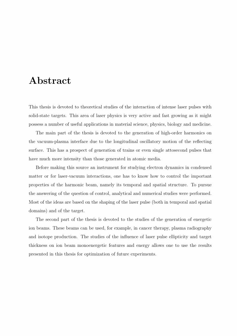
is the diffraction length of the beam. Figure 2.4 shows the results of the propagation of

gaussian beams with ρ0 = 2 (a) and ρ0 = 3 (b) obtained from the numerical simulations

(grayscale image) and from the formula 2.27. The results show good agreement between

simulations and theory.

2.2.3 Numerical scheme for equations of motion.

For the numerical integration of equations of motion the Boris scheme [103] is used (which

is also described by Lichters [100]). First the half-acceleration in electric field only is

applied giving


x, wavelengths

y, w

avel

engt

hs

10 20 30 40 50

−10

−5

0

5

10

(a)

x, wavelengths

y, w

avel

engt

hs

10 20 30 40 50

−10

−5

0

5

10

(b)

Figure 2.4: Propagation of gaussian beams with ρ0 = 2 (a) and ρ0 = 3 (b) in vacuumaccording to simulations (grayscale) and the formulas of gaussian optics (dashed lines).

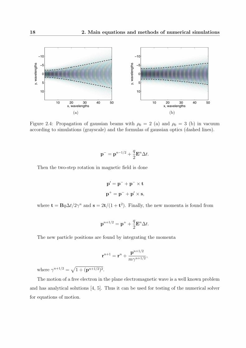
p− = pn−1/2 +q

2En∆t.

Then the two-step rotation in magnetic field is done

p = p− + p− × t

p+ = p− + p × s,

where t = Bq∆t/2γn and s = 2t/(1 + t2). Finally, the new momenta is found from

pn+1/2 = p+ +q

2En∆t.

The new particle positions are found by integrating the momenta

rn+1 = rn +pn+1/2

mγn+1/2,

where γn+1/2 =

1 + (pn+1/2)2.

The motion of a free electron in the plane electromagnetic wave is a well known problem

and has analytical solutions [4, 5]. Thus it can be used for testing of the numerical solver

for equations of motion.


10 12 14 160

1

2

3

4

5 x 10−3

t, cycles

p x, rel

. uni

ts

10 12 14 16−0.1

−0.05

0

0.05

0.1

t, cycles

p y, rel

. uni

ts

10 12 14 160

0.02

0.04

0.06

0.08

t, cycles

x, re

l. un

its

10 12 14 16−0.1

−0.05

0

0.05

0.1

t, cycles

y, re

l. un

its

Figure 2.5: Results of the numerical simulations of the free electron motion in the elec-tromagnetic pulse with a0 = 0.1 and FWHM-duration of the electric field TFWHM = 5cycles.


For the electron initially at rest at x0 irradiated by the linear polarized laser pulse

propagating along the x axis the solutions read

x(ξ) = x0 +1

2

a

2y(ξ)

γ(ξ)dξ

t(ξ) = ξ +1

2

a

2y(ξ)

γ(ξ)dξ

py(ξ) = ay(ξ)

px(ξ) =1

2γ(ξ)a

2y(ξ),

(2.28)

where ay(ξ) - is the vector potential of the electromagnetic waves, px, py - the kinemat-

ical momenta components of the electron. The results of the numerical simulations for the

laser pulse with a0 = 0.1 and full-width-half-maximum (FWHM) duration of 5 cycles are

presented on fig. 2.5. In this case the γ - factor in eqns. 2.28 is equal to 1 with high ac-

curacy. Lower-left figure demonstrates the electron drift in the longitudinal direction with

double the laser frequency. Lower-right figure shows the dependance of the y coordinate

(which is simply the integration of py in this case) on time (solid line) as well as the laser

vector potential (dotted line). One can see the phase difference of π/2 as predicted by the

theory.

Upper figures show the evolution of the momenta components px (left) and py (right)

with time obtained from the numerical simulations (solid line) and from eqns. 2.28 (dotted

line). Results of the simulations exhibit good agreement with the analytical solutions.

2.2.4 Current deposition.

By moving, the particles produce currents. As the particle coordinates change continuously

it is important to connect them to the Eulerian grid where the fields are defined. There

are several local numerical current deposition schemes (charge conservation schemes) that

allow to avoid solving the Poisson equation every time step [98, 97]. One of them is called

the zigzag scheme and was proposed by Umeda et al [96].


i1 i1+1j1

j1+1

j

(x1+x2)/2

(y1+y2)/2

Wx!x

Wy!y

(a)

i1 i1+1j1

j1+1j

(b)

i1 i1+1j1

j1+1

j

(c)

Figure 2.6: Current deposition schematics. (a) Particle remains in the same cell; (b),(c)particle changes the cell in both x and y directions. On sub-figure (b) the particle motion isassumed to be a straight line and described as the motion of 3 sub-particles, on sub-figure(c) the particle trajectory is assumed to be a zigzag line and is described by the motion of2 sub-particles.

The continuity equation in discrete form reads

ρ[n+1,i,j] − ρ

[n,i,j]

∆t+

j[n+1/2,i+1/2,j]x − j

[n+1/2,i−1/2,j]x

∆x+

j[n+1/2,i,j+1/2]y − j

[n+1/2,i,j−1/2]x

∆y= 0.

(2.29)

Let’s assume the particle has a rectangular shape and moves from position (x1, y1) to

(x2, y2). Let’s also assume that the point (x1, y1) belongs to the cell with coordinates (i1, j1)

and (x2, y2) belongs to the cell with coordinates (i2, j2). Depending on the end position

of the particle i2 and j2 can be equal to i1 and j1 respectively or be different. Maximum

displacement δ of the particle can not be more than the cell spacings ∆x and ∆y as the

particle can not move faster than with the speed of light in vacuum.

Let’s first discuss the density deposition. As one can see from the schematic drawing

on fig. 2.6a the particle with coordinates (x1, y1) occupies four cells. One can define the

weighting coefficients

Wn

x=

x1 − i1∆x

∆xW

n

y=

y1 − j1∆y

∆y. (2.30)

This coefficients (both less than one) define what part of the particle lies in the certain cell


in the following way

ρ[n,i1,j1] = q · (1−W

n

x)(1−W

n

y) ρ

[n,i1+1,j1] = q · W n

x(1−W

n

y)

ρ[n,i1,j1+1] = q · (1−W

n

x)W n

yρ

[n,i1+1,j1+1] = q · W n

xW

n

y.

(2.31)

Let’s now discuss the current deposition. The simplest case - when the particle remains

in the same cell while moving, is schematically shown on fig. 2.6a. The current is assigned

to four points: jx is assigned to points (i1 + 1/2, j1) and (i1 + 1/2, j1 + 1/2) and jy is

assigned to (i1, j1 +1/2) and (i1 +1, j1 +1/2). The total current density in both directions

is given by

Fx = qvx = qx2 − x1

∆tFy = qvy = q

y2 − y1

∆t(2.32)

and the weighting is done at the time step n + 1/2 - the moment when the particle was in

the middle of its trajectory, thus

Wx =x1 + x2

2∆x− i1 Wy =

y1 + y2

2∆y− j1. (2.33)

The current density is then deposited on the grid in the following way

j[n+1/2,i1+1/2,j1]x

= qFx(1−Wy) j[n+1/2,i1+1/2,j1+1]x

= qFxWy

j[n+1/2,i1,j1+1/2]y

= qFy(1−Wx) j[n+1/2,i1+1,j1+1/2]x

= qFyWx.

(2.34)

When the particle moves across the cell walls, the situation becomes a bit more com-

plicated, but its trajectory can be viewed as a motion of several particles. In the method

proposed by Villasenor and Buneman [98] the particle trajectory is always assumed to be

a straight line. For example on fig. 2.6b the particle motion is described as motion of three

sub-particles, each moving along the straight line with start and end coordinates located

within the same cell. This algorithm has a major drawback as it uses the conditional

operators in its implementation, which generally take a lot of computational time.

Umeda et al. suggested that the particle trajectory ”needs not to be a straight” line

and developed a new charge-conservation scheme called the zigzag method [96]. The idea


behind this method is to separate the motion into the motion of two sub-particles, one

moving from the start to the intermediate point (the relay point) and the other moving

from the relay point to the end position (see fig. 2.6c).

Let’s consider the case when the particle changes the cell in both x and y directions.

Other variants are done in analogy. As shown on fig. 2.6c we split the trajectory of one

particle into the motion of two sub-particles, one moving from (x1, y1) to a relay point

((i1 + 1)∆x, (j1 + 1)∆y), and another one from the relay point to (x2, y2). The particle

trajectory becomes a zigzag-line. For each of the sub-particles we can now repeat the simple

procedure of eq. 2.34. This current deposition scheme is much easier in implementation

than the Villasenor and Buneman scheme and allows to avoid the conditional operators.

All four cases can be united by defining the relay point for each case. For example, in

one-dimensional case, the relay point xr is given by

xr =

x1+x22 if the particle remains in the same cell

max(i1∆x, i2∆x) otherwise,

so the relay point is located either in the middle of the straight-line trajectory if the

particle remains in the same cell, or in one of the grid points i1∆x or i2∆x depending on

the direction of particle motion.

In two-dimensional case Umeda et al show that the relay point can be defined analo-

gously to the one-dimensional case without the conditional operators:

xr = min

min(i1∆x, i2∆x) + ∆x, max

max(i1∆x, i2∆x),

x1 + x2

2

yr = min

min(i1∆y, i2∆y) + ∆y, max

max(i1∆y, i2∆y),

y1 + y2

2

.

The current density is then decomposed into

Fx1 = qxr − x1

∆t, Fy1 = q

yr − y1

∆t

Fx2 = qx2 − xr

∆t, Fy1 = q

y2 − yr

∆t.


Maxwell equation solverfinds new field values

Linear interpolation offields to the particle position

Equations of motion solver pushes theparticles

Current deposition

Figure 2.7: The routine of one time step in the particle-in-cell code.

Combined with the linear weighting coefficients

Wx1 =x1 + xr

2∆x− i1, Wy1 =

y1 + yr

2∆y− j1

Wx2 =xr + x2

2∆x− i2, Wy2 =

yr + y2

2∆y− j2.

the currents at 8 grid points can be obtained from

j[i1+1/2,j1]x

= Fx1(1−Wy1), j[i1+1/2,j1+1]x

= Fx1Wy1

j[i2+1/2,j2]x

= Fx2(1−Wy2), j[i2+1/2,j2+1]x

= Fx2Wy2

j[i1,j1+1/2]y

= Fy1(1−Wx1), j[i1+1,j1+1/2]y

= Fy1Wx1

j[i2,j2+1/2]y

= Fy2(1−Wx2), j[i2+1,j2+1/2]y

= Fy2Wx2 .

By obtaining the currents one time step ends and the next one starts again with solving

the Maxwell equations using new currents values. Thus one time-cycle of the particle-in-cell

method can be schematically drawn as on fig. 2.7.

2.2.5 Decay of the electromagnetic wave in the skin layer of the

overdense plasma.

For testing the operation of all four routines of the PIC code one can use the known law

of decay of electromagnetic waves in the overdense plasmas. In the case of non-collisional

2.3 Summary of the chapter 25

120 122 124 126 128 130

!0.1

!0.05

0

0.05

0.1

x, rel. units

Ey, r

el.

un

its

Figure 2.8: Results of the numerical simulations showing the decay of the electromagneticfield with a0 = 0.1 inside the overdense plasma with density n = 4. Dashed line outlinesthe vacuum-plasma interface, solid line shows the electric field of the incoming (from leftto right) laser pulse and red circles are obtained from eq. 2.35.

plasma its dielectric permeability is in simple case given by

ε(ω) = 1− n

ncr

= 1−ω

2p

ω2,

where n is the plasma density and ncr is the critical density (the density for which the

plasma frequency ωp =√

n is equal to the electromagnetic wave frequency). This de-

pendance of permeability on frequency ω leads to the well-known exponential decay for

ω < ωp

Ey(t, x) = A · eiωt · e−xls , (2.35)

where ls = 1/ωp = 1/√

n is the skin depth.

The comparison of the PIC simulation resuls (solid line) with the formula 2.35 (red

circles) is shown on fig. 2.8. It exhibits good agreement.

2.3 Summary of the chapter

In this chapter the main equations and methods of numerical simulationts are described.

According to the numerical schemes described above the numerical code PICWIG was


written that allows to simulate the interaction of intense laser pulses with collisionless

fully-ionized plasma in 1D and 2D geometries. All the simulation results presented in this

thesis were obtained using this code.

Chapter 3

Generation of high-order harmonics

on the plasma-vacuum boundary.

3.1 Oscillating Mirror (OM) harmonics

3.1.1 One-particle mirror model

Albert Einstein [104] showed that the reflection of electromagnetic wave from a moving

mirror results in a frequency shift of (1 + β)/(1 − β) with β the speed of the mirror. If

the mirror moves periodically, for example with the period of the incoming wave, than

constructive and destructive interference would lead to the appearance of the spectrum

exhibiting harmonics of the fundamental wave frequency. This scenario is happening when

a relativistically strong laser pulse is incident onto the overdense plasma surface, where

surface oscillations arise as a result of the interplay between laser pressure and the restoring

force from the ions. This simple concept of oscillating surface was proposed by Bulanov et

al [31] and became a working horse in explanation of the phenomena. It was later followed

by the detailed discussions by Lichters et al [105], Tsakiris et al [106], Gordienko et al [107]

and Baeva et al [108].

In order to understand the basic properties of the surface motion one can use the

simple one dimensional one particle model, which describes the longitudinal motion of the

28 3. Generation of high-order harmonics on the plasma-vacuum boundary.

Figure 3.1: One-particle plasma surface model schematics showing the plasma-vacuuminterface. The laser pulse is normally incident from the left side, part of it is reflected andpart of it decays in the skin-layer of the target. Separation of the electrons from the ionsresults in longitudinal electrostatic field proportional to the separation length d.

incompressible electron layer relative to the immobile ion layer under the influence of the

linearly polarized laser pulse incident normally. From the Poisson equation it is easy to

find that the charge-separation potential is proportional to x2, where x - is the electron

layer displacement. The Lagrangian of such a system in relativistic units reads

L(t, x, βx, βy) = −

1− β2 − ay(t, x) · βy − 0.5 · n · x2, (3.1)

where ay(t, x) is the driving vector potential and n is the plasma density which de-

fines the restoring force. Similar models were used by Zaretsky et al [109] for studies of

Landau damping in thin foils and by Mulser et al [110] for studies of the laser absorption

mechanisms.

First we note that Lagrangian (3.1) does not depend on the transverse coordinate y

thus leading to the momentum conservation

py = ay(t, x). (3.2)

Using the Euler-Lagrange equation one can obtain the equation of motion

dpx

dt= −βy

∂ay

∂x− nx. (3.3)

3.1 Oscillating Mirror (OM) harmonics 29

Using the equation for energy variation

dγ

dt= βy

∂ay

∂t− βxnx,

and the connection βx,y = px,y/γ, left part of eq. (3.3) can be rewritten in the following

formdpx

dt=

d(γβx)

dt= γ

dβx

dt+ βx

dγ

dt=

= γdβx

dt+ βx

βy

∂ay

∂t− βxnx

= γ

dβx

dt+

βx

2γ

∂a2y

∂t− β

2xnx.

Thus, eq. (3.3) after transformations reads

dβx

dt= − 1

2γ2

∂a

2y

∂x+ βx

∂a2y

∂t

− nx

γ(1− β

2x) (3.4)

Representing the gamma-factor in the form γ =1 + a

2y

/ (1− β

2x), we get an equation

for coordinate x

x = − 1− x2

2(1 + a2y)

∂a2

y

∂x+ x

∂a2y

∂t

− nx(1− x

2)3/2

1 + a2

y

(3.5)

with initial conditions

x(0) = 0

βx(0) = 0.(3.6)

In equation 3.5 ay is the driving vector potential which is the result of the interference

between the incoming and reflected light. In the following we assume that plasma surface

possesses 100 percent reflectivity.

If one takes the incoming vector potential ai

y(t, x) in the form a

i

y(t, x) = −Ei ·sin(t−x),

then electric and magnetic fields are given by expressions

Ey,inc = Ei · cos(t− x)

Bz,inc = Ei · cos(t− x).


For the reflected light one can write

Ey,refl = Er · cos(t + x + φr)

Bz,refl = −Er · cos(t + x + φr),(3.7)

and for transmitted light

Ey,trans = Et · cos(t + φt) · e−x−xp

ls

Bz,trans =Et

ls· sin(t + φt) · e−

x−xpls ,

where ls = 1/ωp = 1/√

n - is the depth of the skin-layer, ωp > 1 is the plasma frequency.

As the boundary condition one can use the continuity of the electromagnetic fields on the

plasma-vacuum boundary (x = xp):

Ei · cos(t− xp) + Er · cos(t + xp + φr) = Et · cos(t + φt)

Ei · cos(t− xp)− Er · cos(t + xp + φr) =Et

ls· sin(t + φt)

Using the formulae of trigonometry one gets the following values for amplitudes and

phases

Ei = Er

Et =2Ei1 + ω2

p

φt = α− xp

φr = 2(α− xp),

where α = arctan(ωp).

Formally, in the relativistic case we are not allowed to use the simple expression for the

skin-depth ls = 1/ωp and have to take into account the relativistic corrections. However,

from the expression for Et we see that the plasma screens the incoming field and the

amplitude of the field on the surface is ωp times lower than the amplitude of the incoming


light. Thus the linear expression for the skin-depth can be used when a0 < ωp. When the

amplitude a0 exceeds ωp, the relativistic correction to the skin-depth can be made taking

into account the change of the electron energy

ωp =

√n

√mγ

=

√n√

γ

ls =

γ

n

γ ≈

1 + E2t

(3.8)

The field on the plasma surface is the result of the interference of the incoming and

reflected light

Edr = Erefl + Einc = Ei · cos(t− xp) + Ei · cos(t− xp + 2α) =

= 2Ei · cos(t− xp + α) cos α

Bdr = Brefl + Binc = Ei · cos(t− xp)− Ei · cos(t− xp + 2α) =

= 2Ei · sin(t− xp + α) sin α,

(3.9)

thus

Edr =2Ei1 + ω2

p

cos(t− xp + α)

Bdr =2ωpEi1 + ω2

p

sin(t− xp + α)(3.10)

Vector potential inside plasma (for x > xp) can be written in the following form

atrans = − 2Ei1 + ω2

p

sin(t− xp + α) · e−ωp(x−xp) (3.11)

Vector potential driving the surface can be obtained from eq. 3.11 by putting x = xp.

Using the trigonometry formulae eq. (3.5) can be rewritten in the form

x = (1− x2) · Fdr − nx(1− x

2)3/2 · Fr (3.12)

where Fdr = (2E2iωp [1− cos (2(t− xp + α)− θ)]) /

(1 + a2

dr)(1 + ω2

p), and Fr = 1/

1 + a2

dr.


When x 1 this equation allows the analytical solution. In this case eq. (3.12) reads

x + nx =2E2

iωp

1 + ω2p

(1− cos 2τ), (3.13)

where τ = t− xp + α. From this equation the amplitude of the longitudinal oscillations X

for small a0 can be easily obtained

X =2E2

i

√n

(1 + n)(n− 4)+

2E2i

√n

n(n + 1)≈ 2E2

in−3/2

. (3.14)

In the case when n = 4 formally we can not write the solution in this form, but after

taking into account dissipation in some form we can see the well-known two photon plasma

resonance [55]. Amplitude of the transverse oscillations Y in the case of small a0 is easy

to find from the equation y = ay:

Y =2Ei1 + ω2

p

≈ 2Ein−1/2 (3.15)

In the general case eq. 3.12 requires a numerical solution. Results of the model calcu-

lations are presented on fig. 3.2. Trajectory of the electron during the interaction with the

laser pulse with amplitude a0 = 10 (corresponding to the intensity of 1.37 ·1020 W/cm2 for

the laser with the wavelength λL = 1 µm), with a gaussian envelope and a 4-cycles FWHM

duration is shown on fig. 3.2a. Plasma density is ne = 400. Fig. 3.2b shows the transverse

coordinate ye as a function of time t. On fig. 3.2c the solid line shows the longitudinal

coordinate xe (horizontal axis) as a function of time t (vertical axis).

Dependance of the amplitude of the longitudinal X and transverse Y electron motion

on the laser pulse amplitude a0 for plasma density ne = 400 are shown on fig. 3.3. On both

figures the diamonds represent the result of numerical solutions of the model equations

and dashed lines represent low a0 asymptotic solutions (eqns. 3.14 and 3.15). On fig. 3.3a

the circles show the results of the model with the relativistic skin-layer corrections taken

into account. The simple estimates of eqns. 3.14 and 3.15 work well until the value of

approximately a0 = ωp/2. After that the relativistic corrections to the skin depth and


!0.1

0

0.1y,

wa

vele

ng

ths

t, p

erio

ds

x, wavelengths

!0.005 0 0.005 0.01

5

10

0 5 10t, periods

a) b)

c)

Figure 3.2: Electron motion obtained using the single particle model for laser pulse witha0 = 10 with 4 cycles FWHM-duration and ne = 400. Electron is initially located atxe = ye = 0. Subfigure (a) shows the electron trajectory, subfigure (b) demonstrates thebehaviour of the transverse coordinate ye in time, on subfigure (c) the dashed line representsthe longitudinal coordinate xe of the electron (vertical axis) versus time (horizontal axis)obtained from the model, the color coded image displays the spatio-temporal picture of theelectron density obtained from 1D-PIC simulations with same laser and plasma parameters.

electron longitudinal motion become important.

In order to check the validity of the afore-described model we have conducted a series

of 1D PIC simulations. The code described in Chapter 2 allows the simulation of the

interaction of the intense laser pulses with pre-ionized non-collisional plasma. The density

in the simulations is n = 400, step-like vacuum-plasma interface is assumed, the ions are

immobile. Throughout the thesis we use FWHM of the electric field as the definition of the

laser pulse duration and use pulses with an electric field that has a Gaussian envelope func-

tion. The results are presented on fig. 3.2 and fig. 3.3. The color-coded image on fig. 3.2c

presents the spatio-temporal picture of the electron density obtained from simulations with

the same laser and plasma parameters as in the model (solid-line). One can see that the

model is in perfect agreement with the PIC simulations. Fig. 3.3a,b show the amplitude

of electron longitudinal X and transverse Y oscillations respectively as a function of a0


0 5 10 15 200

0.002

0.004

0.006

0.008

0.01

0.012

a0, rel. units

X, w

avel

engt

hs

(a)

0 2 4 6 8 100

0.05

0.1

0.15

0.2

a0, rel. units

Y, w

avel

engt

hs

(b)

Figure 3.3: Amplitudes of longitudinal (a) and transverse (b) oscillations as functions oflaser amplitude a0. On both subfigures diamonds represent the numerical solutions ofthe model equations, squares represent the results of the PIC simulations, dashed lines- the results of the analytical solutions of the model equations for low a0. On subfigure(a) the circles are obtained from numerical solutions of the model equations including therelativistic corrections to the skin-depth, solid line represents the capacitor model. Plasmadensity is n = 400.

Figure 3.4: Schematics of the capacitor model.

obtained from PIC simulations (squares). The fact that the simulation results lie on the

curve obtained from the model and as longitudinal motion is directly correlated to the

transverse motion allows us to claim that the model works well and gives correct results

for both longitudinal and transverse coordinates. Latter are hard to obtain from 1D PIC

simulations as the particles leave the interaction region and are very intricate to trace.

It is interesting that the amplitude of the longitudinal oscillations X can be found from

a different point of view - using the balance of the longitudinal charge-separation field and

laser pressure. Laser pressure leads to the displacement and compression of the electron


layer inside the target to the depth d (see fig. 3.4). The density of the compressed electron

layer is denoted as ncompressed, the characteristic size of the compressed layer is equal to

the skin depth ls. Writing down the condition of plasma neutrality we get

ncompressed · ls = n0 · (d + ls). (3.16)

Electrostatic field that arises when the electron layer is displaced by the length d is

given by Ees = n0 ·d, where n0 is initial plasma density. Writing down the balance between

laser pressure and electrostatic pressure we obtain

ncompressed · ls · n0 · d2

= (1 + R)E20 ≈ 2E2

0 , (3.17)

where R is the reflection coefficient which is assumed to be unity. Using eq. 3.16 we get

the following equation for displacement d:

d2 + ls · d−

4E20

n20

= 0, (3.18)

with the solution in the following form

d = − 1

2√

n0+

1

2

1

n0+

16E20

n20

. (3.19)

Amplitude of longitudinal surface oscillation obtained from this (capacitor) model is

shown on fig. 3.3a with a solid line. The results of PIC simulations, the simple mirror

model and the capacitor model are in perfect agreement. Capacitor model is later used in

this thesis for studies of the ion acceleration process.

3.1.2 Emission of harmonic spectrum.

The simple one particle model described above allows to understand the generation of

high-order harmonics from both macroscopic and microscopic points of view.


Taking into consideration only the longitudinal motion of the surface and applying the

boundary conditions for reflected light from eq. 3.7 one gets for reflected electric field

Erefl = Ei · cos(t− x(t) + 2α), (3.20)

where t = t + x(t) is the ”meeting” time of the wave and the electron. Presence of

the nonlinear term x(t) inside the cosine function makes the right part of this equation

nonlinear and exhibits harmonic spectra if x(t) is periodic. For the spectrum of the

reflected light one can write

E(q) =Ei

2√

2π

∞

−∞e

i(t−x(t)+2α−qt)dt + c.c. (3.21)

The behavior of this integral for high frequencies q 1 and high mirror velocities (ap-

proaching the speed of light) does not depend on the exact mirror motion function x(t)

and can be found using the standard asymptotic methods [111]. Gordienko et al [107]

and later Baeva et al [108] showed that the spectrum is universal and exhibits a certain

frequency dependance - it decays proportionally to q−5/2 or q

−8/3. Moreover, the spectrum

extends up to a certain cut-off frequency ωco that is proportional to the γ3, where γ is the

relativistic gamma-factor of the mirror, followed by the exponential roll-off. The integral

in eq. 3.21 can also be taken numerically assuming the mirror motion function x(t) in

some form as shown in the paper by Tsakiris et al [106]. It shows the same frequency de-

pendance and the cut-off frequency. As the moments when the surface moves towards the

laser and has the highest longitudinal velocity are strongly localized in time, the Doppler

shift produces a flash of harmonics with the attosecond duration [106].

Another way of looking at the emission of harmonics is from a more microscopic point of

view. Although the model described above deals with the incompressible electron layer and

not with the individual microscopical electron, we can assume that all the electrons within

the skin layer are doing the same arc-like trajectories. Given the trajectory of the electron

one can find the radiation it produces with the help of Lienard-Wiechert potentials [4].

Electric field is given by the following expression


E(xd, t) = −(n− β)(1− β2)

κ3R2

ret

− n

κ3R× ((n− β)×w)

ret

, (3.22)

where xd - is the position of the detector, n = R/R, where R is the radius vector pointing

from the detector to the particle, β and w are the electron velocity and acceleration

respectively and κ = 1− nβ. The quantities in square brackets are taken in the retarded

time. For large distances we can neglect the first term in the right part of eq. 3.22 as it

scales with R2 and is not responsible for the generation of electromagnetic waves [4]. As

for the second part, we have to remember that the surface in 1D case is infinite in the

transverse direction, so we only look at the transverse electric field component Ey and

put a detector at position with yd = 0 (the electron is supposed to be initially at rest at

x = 0, y = 0). For R 1 one can set nx = 1 and ny = 0 and write for Ey(xd, t)

Ey(xd, t) = E0 · [wy · (1− βx) + wx · βy]ret, (3.23)

where E0 ≈ 1/κ3R. All functions on the right side of the equation are nonlinear as they

depend on t = t + x(t). This leads to emission of harmonic spectrum. For example, for

non-relativistic mirror motion case wy is the analogue to the electric field on the surface

(wy = py = ay) and has the same form as in eq. 3.20.

Equation 3.23 can be solved numerically for arbitrary electron trajectories. As a test

one can numerically solve eq. 3.23 for an electron oscillating with a certain frequency only

in transverse direction y and assure the well-known cos2(θ) law for angular distribution [4].

Figure 3.5a shows the results of the numerical solution of eq. 3.23 (circles) compared with

the cos2(θ) formula (solid line) and exhibits perfect agreement. The dipole oscillating in

transverse direction with fundamental frequency radiates at the same frequency. As the

electron starts slightly wiggling in the longitudinal direction the radiation exhibits a broad

spectrum. From fig. 3.2c one can see that the electron amplitude in longitudinal direction

is not high and so is the amplitude of the longitudinal velocity. Nevertheless, the nonlinear-

ity due to the longitudinal motion is enough to produce the harmonic spectrum, although

not at the highest efficiency compared to the case of relativistically moving mirror [108].


0.2

0.4

0.6

0.8

1

30

210

60

240

90

270

120

300

150

330

180 0

(a)

0 5 10 15 20 25

100

ω/ωL

Nor

mal

ized

inte

nsity

(b)

8 8.5 9 9.5 10 10.5 110

0.2

0.4

0.6

0.8

1

Time, periods

Nor

mal

ized

inte

nsity

(c)

Figure 3.5: a) Angular distribution of the intensity of emitted light for the case of dipoleoscillating in y direction. Dots represent the results of calculations using Lienard-Wiechertformula and the straight line is the predictions of the theory. b) Spectrum emitted by theparticle moving with the trajectory same as on fig. 3.2a. c) Results of filtering (from 9thto 19th harmonics) of the light emitted by the particle.

Fig. 3.5b demonstrates the spectrum radiated by the electron moving with the same tra-

jectory as on fig. 3.2a and exhibits only odd harmonics of fundamental frequency as the

periodicity of the longitudinal oscillations is double the fundamental frequency. Detector is

placed far on the left from the initial electron position. Fig. 3.5c demonstrates the results

of the filtering of harmonics from 9th to 19th. A train of attosecond pulses is clearly visible.

One can put a detector also to the far right from the electron and observe approximately

the same picture. This explains the harmonic emission from the rear side of the foils.

In the simple model the plasma is not present and the rear side spectrum exhibits all

odd harmonics from fundamental up to the highest. In reality plasma would filter out

all harmonics below the plasma frequency - this is in perfect agreement with the PIC

simulations.

3.2 Summary of the chapter.

In this chapter the simple one-particle model is presented. This model is very intuitive and

allows to understand the basic properties of the dynamics of the reflecting surface during

the interaction with intense laser pulse. A series of PIC simulations exhibit good agreement

with the model calculations. It is shown that for the case of normal incidence of the laser

3.2 Summary of the chapter. 39

pulse the term relativistic interaction is very relative and depends on the intensity of the

pulse as well as density of the target. A plasma with higher density effectively screens the

incoming laser pulse. The emission of harmonic spectrum happens due to the nonlinear

and periodic term and can be understood from both macroscopic and microscopic points

of view.

Chapter 4

Controlling the temporal structure of

harmonic beam.

The most straightforward way of generating the attosecond pulses is by slicing a part of

the reflected spectrum by a bandpass filter that suppresses the fundamental and low lying

harmonics. If the driving pulse is a many-cycle laser pulse (consisting of several periods

of the 2.63 fs period for a commonly used Ti:sapphire laser systems), the plasma mirror

executes accordingly also oscillations and the process is repetitive. This gives rise to a

discrete spectrum within the filtered part, which in the time domain corresponds to a

train of attosecond pulses. For many applications a single attosecond pulse is desirable

[49]. The simple mirror model concept gives two possibilities for pursuing this goal. Both

methods rely on reducing the number of surface oscillations during interaction. The most

straightforward idea is to use laser pulses that have the duration of only few cycles (ideally

only one cycle) - thus during the interaction the surface oscillates only few times and

single attosecond pulse can be extracted. This method is called intensity gating and was

theoretically studied, for example, in the paper by Tsakiris et al [106]. Let us briefly

discuss this method.

42 4. Controlling the temporal structure of harmonic beam.

(a) (b)

Figure 4.1: Instantaneous intensity of 2-cycle cosine (a) and sine (b) pulses.

4.1 Intensity gating

In the intensity gating technique in order to properly extract a single attosecond pulse

from the harmonics generated on the surface it is important to control the carrier-envelope

phase (CEP) of the incoming pulse. This becomes obvious from a schematic drawing on

fig. 4.1 where the instantaneous intensity of cosine (a) and sine (b) pulses is presented. For

cosine pulse it is possible to gate only one peak, whereas the sine pulse always has two

peaks in intensity.

From eq. 3.9 electric field driving the surface is given by

Edr(t) = E0,dr · cos(t + α + φ0), (4.1)

where E0,dr - is the amplitude, α = arctan(ωp) and φ0 is the CE-phase. Let’s fix the

plasma density n to 81 times overcritical. Plasma frequency ωp is then equal to 9 and

α = 1.46 ≈ π/2, which means that it is not optimal to shoot cosine pulse initially, but

rather a pulse with phase φ0 = −α. Spectrum of the 2-cycle pulse with amplitude a0 = 20,

reflected from the plasma with density n = 81 is shown on fig. 4.2a. When initial CE-phase

φ0 was set to 0 corresponding to the cosine-pulse, filtering of the reflected light from 30th

to 100th harmonic resulted in a train of 2 attosecond pulses (fig. 4.2b). In the optimal case

when the CE-phase was set to compensate α the filtering resulted in the single attosecond

4.2 Polarization gating 43

0 20 40 60 80 10010

!8

10!6

10!4

10!2

100

No

rmal

ize

d in

ten

sity

!/!06 6.5 7 7.5 8 8.5

0

0.2

0.4

0.6

0.8

1

t, periods

No

rmal

ize

d in

ten

sity

6 6.5 7 7.5 8 8.50

0.2

0.4

0.6

0.8

1

t, periods

No

rmal

ize

d in

ten

sity

Figure 4.2: a) Spectrum of the reflected light for laser pulse with a0 = 20, 2-cycle duration,density of the target is n = 81. b) Filtered light (from 30th to 100th harmonic) for thecase when initial phase of the laser pulse was φ0 = 0. c) Same as on b) but φ0 = −α.

pulse with strongly suppressed satellites as shown on fig. 4.2c. It is important to notice

that α depends on the density of the target and changes from α = π/4 for the target with

n = 1 to α → π/2 for n → ∞. Thus, the known dependance of the coefficient α can be

used for optimization of experiments.

4.2 Polarization gating

4.2.1 Dynamics of the reflecting surface under the influence of

light with different polarization.

Another approach for generation of single attosecond pulses is to use many-cycle pulses

and incorporate a time varying switch or gate that allows harmonics emission only during

a very short time interval. A possible switch is based on the dependence of the harmonics

efficiency on the polarization state of the driving pulse. In both cases, since the driving

pulse or the gate can be reduced to a 2-3 periods only, the positioning of the carrier

frequency field under the envelope of the pulse and therefore the carrier-envelope phase

(CEP) stabilization plays an important role.

As shown in previous section, it is possible to generate single attosecond pulses with

the help of intense few-cycle laser pulses. However, the laser systems with the required

specifications are still under development, and more time is needed to make them fully


operational [112]. Most of the high power (10-100 TW) laser systems currently in operation

in several laboratories deliver pulses with a duration of τL 50 fs. For these systems, the

technique known for almost 10 years in connection with harmonics generation from atomic

media - polarization gating [113, 114, 115] appears to be apropos. In this technique, the

laser pulse is appropriately manipulated so that rapid switching between circular and linear

polarizations within the same pulse occurs for a very short time interval thus creating a

gate that temporally confines the harmonics generation process. The same technique is in

principle applicable to harmonics from solid targets [116]. The aim of the present work

is to study in detail the conditions under which the specific polarization gating technique

used in gas harmonics can effectively be applied to surface harmonics. The study of the

dependence of harmonics generation efficiency on the ellipticity of the laser pulse for both

normal and oblique incidence allows us to estimate the parameters under which the gate

would effectively confine the emission in only one attosecond pulse.

The basic idea behind the oscillating mirror model is that the electrons at the plasma

vacuum interface execute forced oscillations near the edge of an immobile step-like ion

background. For near-normal incidence, the oscillations are driven by the light pressure

force Fp of the incident laser pulse arising from v×B term of the Lorenz force. In the case

of linear polarization of the incident pulse, this force varies as Fp ∼ a2L(t) · [1 + sin(2ωL ·

t)], where a2L(t) = IL(t) · λ

2L/(1.37 × 1018Wµm2

/cm2) is the normalized vector potential

envelope. Charge separation and induced electrostatic fields give rise to a restoring force

and thus to surface oscillations. Due to the relativistic Doppler shift, light reflected from

such an oscillating mirror consists of a broad harmonics spectrum. Moreover, the harmonics

are generated only during the short time when the mirror moves towards the laser pulse,

which results in their phase-locking and attosecond duration. In the case of the circularly

polarized pulse the force due to light pressure is of the form Fp ∼ a2L(t) and thus it exhibits

no fast oscillations. The slowly-varying laser pressure following the envelope of the laser

pulse pushes the electrons against the restoring force due to charge separation creating

only a dent in the electron cloud. The absence of surface oscillations means also absence

of harmonics emission. These basic assumptions of the oscillating mirror model are clearly


time

normal space coordinate

(a) (b) (c)

3TL

!"# !"#!"#

Figure 4.3: Plasma surface motion (vertical axis represents the time and horizontal axis thespace coordinate both in arbitrary units) under the influence of linearly (a), circularly (b),and (c) gated pulses. In the case of linear polarization (a) surface oscillations (red color)are clearly seen. The generated train of attosecond pulses propagating with the speed oflight are shown in yellow color. Circular polarization (b) exhibits no oscillations and asa consequence no harmonics are generated. In the case of a polarization gated pulse (c)the surface oscillations are highly suppressed during the time of circular polarization andonly few of them survive. One clearly sees that only one attosecond pulse is generated.The simulation parameters are: aL = 10 (IL = 100Irel ≈ 2.0 · 1020 W/cm2

, λL = 0.8 µm),τL = 5 cycles (15 fs), ne = 40ncr, normal incidence.

supported by the 1D-PIC simulations shown in fig. 4.3, where the motion of the surface

under the influence of linearly and circularly polarized light has been calculated.

Now as the basic features of the plasma-vacuum interface motion and the accompa-

nying harmonics generation have been described, the idea of polarization gating becomes

straightforward. When the polarization over the pulse duration rapidly evolves from cir-

cular to linear and back to circular then the harmonics will be generated only during the

linear period, and the shorter it is - the less attosecond pulses will be generated. It is even

possible to gate only one attosecond pulse.

The polarization gating technique was first proposed by Corkum et al. [113] along

with a technique of using two pulses with slightly different frequencies to generate the

polarization gate. Platonenko and Strelkov [114] proposed to use only linear optics to

construct a gate, and this idea was experimentally realized by Tscherbakoff et al. [115].

The shortest attosecond pulses from atomic medium (130 attoseconds) were produced using

this technique by Sansone et al. [117]. The polarization gating technique was also discussed


!"#L(1/v -1/v )e oL45°

Optical axis Optical axis

Quartz plate $%& plate

Figure 4.4: A technique for generating a pulse with time-varying ellipticity. The firstcrystal plate (the optical axis is set to 45 degrees with respect to the initial polarization)splits linearly polarized pulse into two delayed pulses linearly polarized in two mutuallyperpendicular planes. The thickness of the plate is chosen in a such a way as to dephasethe two pulses proportionally to (2n + 1) · π/2 (n is a natural number) so that the plateserves as the multiple order quarter wavelength plate (∆t = L(1/ve − 1/vo), where L isthe thickness of the plate, ve and vo are the velocities of extraordinary and ordinary com-ponents, respectively). The field after the first plate is linearly polarized in the beginningand in the end and has circular polarization in the middle. The second plate (the opticalaxis is set 45 degrees with both components) serves as a 0-order quarter wavelength plateand transforms linear polarization into circular and vice versa.

for the surface harmonics [116]. In view of forthcoming experiments, we restrict ourselves

to studying the experimentally most common technique based on two crystal plates (see

Figure 4.4) and we investigate the details associated with the application of this technique

to the surface harmonics.

4.2.2 Dependance of harmonics generation efficiency on elliptic-

ity

The study of the behavior of harmonics generation efficiency as a function of ellipticity

of the incident pulse allows us to define the gating time. We call gating time - the time

interval when the efficiency of a certain range of harmonics lies above the value of 0.1 of

its maximum. The ellipticity corresponding to this harmonic efficiency is the threshold

ellipticity 0.

As it was already mentioned, the harmonics generation becomes less efficient as the


amplitude of the linearly polarized part decreases with the growth of ellipticity. In order

to determine the threshold ellipticity 0 one has to calculate the harmonic efficiency (for a

single harmonic or a range of harmonics) as a function of ellipticity. The efficiency within

the spectral range between the nth

1 and nth

2 harmonics is given by:

ηn1,n2 =

n2

n1 |Erefl(n)|2dn∞0 |Erefl(n)|2dn

(4.2)

where |Erefl(n)|2 is the reflected spectrum and∞

0 |Erefl(n)|2dn is approximately the in-

cident pulse energy. Figure 4.5 shows the results of the PIC simulations for the efficiency

as given by Equation 4.2 as a function of ellipticity of the incident pulse in the range from

10th to 20th harmonics for aL = 10 and in the range from 20th to 100th harmonics for

aL = 20. From Figure 4.5 one can see that the harmonics lose 90% of efficiency near the

value of threshold ellipticity 0 = 0.4 for aL = 10 and 0 = 0.2 for aL = 20, respectively. We

performed several PIC simulations showing that the value of ellipticity at which the har-

monic efficiency is reduced by 90% slightly changes with the parameters of the laser pulse,

plasma density, and the harmonics range, but we find the value of threshold ellipticity

0 = 0.4 to be an adequate estimate for effective gating.

For the polarization gating scheme shown on Figure 4.4, the evolution of ellipticity with

time is given by:

(t) = exp

−4 ln 2 · |(t−∆)2 − t2|

τ 2L

(4.3)

where ∆ is the delay between two mutually perpendicular field components produced by

the first plate (see Figure 4.4). Given the value of the threshold ellipticity 0, the width of

the ellipticity curve (the gating time) is given by:

δgating =| ln(1− 0)|

4 ln 2· τ

2L

∆(4.4)

For a threshold ellipticity value of 0.4 the formula (4.4) yields:


norm

aliz

ed

harm

onic

effic

iency

0

0.2

0.4

0.6

0.8

1.0

0 0.2 0.4 0.6 0.8 1.0ellipticity

PICresults

a nL

=10, =10-20

a nL

=20, =20-100

Figure 4.5: Dependence of harmonics generation efficiency on the ellipticity of the incidentpulse for two cases: aL = 10 (IL = 100Irel ≈ 2.0·1020 W/cm2

, λL = 0.8 µm) (red diamondsand red dashed curve) and aL = 20 (IL = 400Irel ≈ 9 · 1020 W/cm2

, λL = 0.8 µm) (bluesquares and blue dashed curve). The points are the results of the PIC simulations, whilethe curves are fits to guide the eye.

δgating =0.2τ 2

L

∆(4.5)

In order to keep the gating time constant (5 fs) when increasing the pulse duration, one

has to increase the delay produced by the first plate according to (4.5) (see Figure 4.4).

Figure 4.6 also shows the amplitude of the electric field in the region of linear polarization

(blue color). As one can see the delay needed for a 5 fs gating time increases with increase

of laser pulse duration, and the amplitude decreases dramatically. This is also depicted in

Figure 4.6 where the normalized field amplitude for the two perpendicular components is

shown for three selected pulse durations. We estimate that the maximum reasonable pulse

duration for polarization gating using 2 plates is about 50 fs. For longer pulses, there is

at least a loss of 1 order of magnitude in the region of linear polarization and the energy

waste makes this scheme inefficient. Such a limitation, however, can be overcome by using

a different polarization gating scheme, for example one based on the double Michelson

interferometer [118, 119].


no

rma

lize

dfie

lde

lect

ric

am

plit

ud

e

0.5

1.0

0

0.1 level

de

lay

ne

ed

ed

for

5fs

ga

te(f

s)

400

200

0

pulse duration (fs)0 20 40 60 80 100

norm

aliz

ed

ele

ctric

field

0

0.5

-0.5

-1.0

1.0

ellipticity

Ez

Ey

-30 -10 0 10 20 30-20

t (fs)

0

0.5

-0.5

-1.0

1.0

-30 -10 0 10 20 30-20

t (fs)

ellipticity

Ez

Ey

0

0.5

-0.5

-1.0

1.0

-30 -10 0 10 20 30-20

t (fs)

ellipticity

Ez

Ey

Figure 4.6: Delay needed for a 5 fs gate as a function of incident pulse duration (redcurve) and the amplitude in the linear region of the pulse for this delay (blue curve). Forselected pulse durations, the amplitude of the two field components are shown along withthe variation of ellipticity in the lower panel. Within the polarization gate one of them isreduced to a level that renders a value for the ellipticity below the threshold.


4.2.3 Results of the simulations of the polarization gating

The results of the simulations are summarized in Figure 4.7. The initial pulse duration is 7

cycles (19 fs) and the delay (15 fs) is chosen in a way to keep the gating time approximately

equal to 5 fs. One clearly sees the train of attosecond pulses generated in the case of the

linearly polarized laser pulse, whereas, in the case of the pulses with polarization gating,

practically all the attosecond pulses but one are suppressed and thus the polarization

gating effectively works as a 2-cycle laser pulse. The surface motion in this case is shown

in Figure 4.3c. The wavelet analysis [120] depicted in Figure 4.7 shows also that the use of

higher-frequency filtering allows to generate single attosecond pulse with better contrast

by more effectively suppressing the satellites. As it was mentioned above, the harmonics

are phase-locked due to the mechanism of generation, and owing to the repetitiveness of

the process they give rise to a train of attosecond pulses. When polarization gating is

applied, one should be able to see its effect on the spectrum of the reflected light. If a

single attosecond pulse is thus produced, the discrete spectrum should turn to continuous.

But even if few attosecond pulses are captured by the gate, a broadening of the individual

harmonics should be visible. Figure 4.7 depicts this difference in the spectrum for linear

polarization and polarization gating. One can clearly see the broadening of the individual

harmonics.

4.2.4 Dependence of harmonics generation efficiency on the an-

gle of incidence

All the results described above are obtained for the case of normal incidence of the laser

pulse. However in experiments for practical reasons, e.g., to avoid back reflection into the

laser chain or to provide access to diagnostic instruments, the angle of incidence with re-

spect to the target normal should differ from zero. The question arises whether polarization

gating works as well for oblique incidence. It is well known that even circularly polarized

light generates harmonics when incident obliquely [105] as there is a component of electric

field parallel to the normal that drives surface oscillations. With increase of the angle of


time (fs)

20

30

40

50

ha

rmo

nic

ord

er

(a)

10-410-610-8

normalized intensity

1

0

-1

rel.

inte

nsi

ty

-25 -20 -15 -10 -5 5 15 20 25100

time (fs)

20

30

40

50

ha

rmo

nic

ord

er

-25 -20 -15

(b)

-10 -5 5 15 20 25100 10-510-10

normalized intensity

1

0

-1

rel.

inte

nsi

ty

Figure 4.7: Results of particle-in-cell simulations with parameters: aL = 20 (IL = 400Irel ≈9 · 1020

W/cm2), τL = 7 cycles (19 fs), ne = 80ncr and normal incidence for linear p-

polarization (a) and pulse with polarization gating (b). On both figures the color codedimage shows the wavelet analysis (time-frequency analysis) with the vertical axis as thefrequency axis and the longitudinal axis as the time axis. The graph on the right ofthe image represents the spectrum of the reflected light with frequencies on the verticalaxis and normalized intensity on the longitudinal axis. The graph at the top shows thereflected light (blue color) and the filtered pulse (20-100 harmonics, red color). For thecase of polarization gating (b) the ellipticity evolution (black color) and the gating time(green rectangle) are also shown.


0 10 20 30 40 500.0

0.2

0.4

0.6

0.8simulationlinear fit

thresholdellipticity

angle of incidence (degrees)

0 10 20 30 40 500.0

0.2

0.4

0.6

0.8

simulationlinear fit

thresholdellipticity

angle of incidence (degrees)

10th-20thharmonics

0 10 20 30 40

angle of incidence

(degrees)

0.5

1.0ellipticity

(a)efficiency

0

10-6

10-5

10-4

10-3

10-2

10-1

10-7

0 10 20 30 40

angle of incidence

(degrees)

0

0.5

1.0ellipticity

20th-100thharmonics(b)

efficiency

10-6

10-5

10-4

10-3

10-2

10-1

10-7

10th-20thharmonics

20th-100thharmonics

Figure 4.8: Harmonics generation efficiency as a function of both ellipticity and angle ofincidence. Parameters of the simulations are the same as on Figure 4.7. The incident fieldfor = 0 is p-polarized. Results for harmonics within the range from 10th to 20th (a), andfrom 20th to 50th (b) are presented. For both ranges, the threshold ellipticity 0 for 10%harmonic efficiency as a function of angle of incidence is shown in the lower part.

incidence θ, this part grows proportionally to sin θ. To see the effect of oblique incidence to

the effectiveness of the polarization gating scheme, we have performed a series of 1D-PIC

simulations for angles of incidence between 0 and 45. The oblique incidence case was

incorporated into the 1D code using a Lorentz transformation to a moving frame in which

the light is normally incident [121]. The efficiency of harmonics generation as a function

of both ellipticity and angle of incidence for two harmonic ranges of practical interest is

shown in Figure 4.8. Two different tendencies of the harmonic efficiency are to be noted

here: first, with the increase of the angle of incidence and for all the ellipticity values it

increases by more than an order of magnitude (see also Ref. [33]) and, second, for large

angles of incidence it becomes less sensitive to the ellipticity. Simulations made with dif-

ferent parameters of laser pulse and plasma show similar results, i.e., the curve of efficiency

as a function of ellipticity becomes broader with increasing angle of incidence, indicating

longer gating width. This trend is depicted in the lower part of Figure 4.8, where the


Figure 4.9: Intensity of the single attosecond pulse (blue color, 20-100 harmonics) as wellas intensity of the incident pulse (red color) and ellipticity (black color) for the simulationwith same parameters as in Figure 4.7 and with angle of incidence θ = 15.

threshold ellipticity (the 10% level efficiency) is seen to increase as function of the incident

angle approximately linearly. It appears that the greater the angle of incidence the higher

the threshold ellipticity and therefore, the less confined in time the gate is. Both harmonic

ranges exhibit the same general behavior, but the higher harmonic range (20th-100th)

appears to be slightly more sensitive to ellipticity variation. For 45 target irradiation,

the 10% efficiency level is reached for 0 ≈ 0.6, and this makes target irradiation under

45 questionable for experimental realization of an adequately short gate. However, it is

experimentally practicable to irradiate the target under 10− 15 in which case the results

of the simulations show that the efficiency of harmonic generation decreases rapidly at

small values of ellipticity, deviating only slightly from the case of normal incidence. Thus

it appears quite feasible even under oblique incidence to generate a gate with duration

short enough to restrict the emission to practically a single cycle. This is confirmed by the

results in the Figure 4.9, where the simulations with parameters as in Figure 4.7, but with

oblique incidence (θ = 15), are shown.



In this chapter methods for controlling the temporal structure of harmonics are discussed

based on reducing the number of oscillations of the reflecting surface. The first method

relies on the intensity gating by few-cycle laser pulses and the second method makes use

of pulses with dynamically changing polarization. The study presented in this chapter

gives estimates for the gating time and thus for the parameters of the experimental set-up

needed for obtaining a 5 fs gate. We find that the polarization gating by means of two

plates has a limitation in the incident pulse duration due to the large delays needed, which

in turn can be overcome by a different scheme (for example using the double Michelson

interferometer technique [118]). It is shown that polarization gating is also feasible for

oblique incidence of the laser pulse, at least for angles of incidence θ < 15, which makes

this scheme a candidate for experimental generation of intense single attosecond pulses

using multi-cycle laser pulses.

In comparison with the gas harmonics, it appears that the method is more suitable

for the case of surface harmonics since the shortcoming encountered with gas harmonics

where the circular part induces unwanted ionization does not play a role in this case. In

addition, the surface oscillations in the case θ > 0 are driven not only by the light pressure

force that oscillates at 2ωL, but also by the normal to the surface component of the electric

field that oscillates at ωL. Subsequently as the angle of incidence increases, a regime is

reached where all harmonics (odd and even) are efficiently generated and the attosecond

pulses in the resulting train appear on every cycle and not every half-cycle as in the case

of gas harmonic (odd orders only). This is a factor that should be taken into account in

determining the optimum angle of incidence since it has the advantage that twice as long

gates can be used to isolate a single attosecond pulse.

Chapter 5

Controlling the spatial structure of

harmonic beam.

In previous chapter methods of controlling the temporal structure of harmonic beam were

presented. Besides the temporal coherence the spatial coherence is of great importance es-

pecially in the view of the possibility of generation of electric fields with extreme intensities

by focussing the harmonic beam to the diffraction limit. Reaching the so-called Schwinger

intensity of 1029W cm−2 [50] would help to open the whole new field of nonlinear quantum

electrodynamics, where the vacuum can not be considered empty and interacts with the

laser light [122, 123, 124, 125]. The Schwinger limit seems hard to reach with conven-

tional laser systems with the wavelength of about 1µm. High-order harmonics are a good

candidate in that direction as besides the short duration they have also short wavelength

and can in theory be focused [53]. From the experimental point of view some questions

immediately arise. What is the divergence of the beam, how can it be controlled and how

is it affected by the impurities of the target? In this chapter we make an attempt to answer

these questions.

56 5. Controlling the spatial structure of harmonic beam.

den

ted

surf

ace

flat

surf

ace

con

stan

td

iver

gen

cew

avel

eng

th-d

epen

den

td

iver

gen

ce

a)

b)

Figure 5.1: Illustration of target denting influence on the harmonic beam divergence. a)Divergence in the case of the planar target - the divergence of each harmonic depends onits wavelength. b) Divergence in the case of dented target - the beam is focused beforediverging with the constant angle. (Figure courtesy R. Horlein)

5.1 Surface denting

In the one-dimensional description of the generation process we always assume that the

target is planar. If the harmonics are generated on a planar surface then the divergence

angle Θq of the q-th harmonic is given by the approximate expression

Θq ∝λq

Dq

, (5.1)

where λq and Dq are the wavelength and the source size of the q-th harmonic respec-

tively. This scaling says that if all the harmonics are generated within the same spot, which

has approximately the size of the laser spot, then the divergence is different depending on

the harmonic wavelength. However, the experiments [28] show different scaling, namely

all harmonics (within the measurement, harmonics from 20 to 40) have the same angle of

divergence. This contradiction can not be resolved by assuming that the harmonics were

generated each with the different initial spot size and another explanation is needed. As it

5.1 Surface denting 57

was mentioned above, expression 5.1 only works in the case of planar target geometry. In

fact, initial planar target geometry changes during the interaction with the intense laser

pulse due to the denting created by the inhomogeneous transverse distribution of the laser

beam. This leads to the generation of the harmonics with curved wavefronts which can ex-

plain the experimental findings. The effect of the surface curvature on the divergence angle

of the harmonic beam is schematically outlined in fig. 5.2. In the planar target geometry

the beam diverges from the target and the divergence angle of each harmonic is governed

by eq. 5.1. In the case of the dented or pre-curved target the harmonic beam first goes

through the focus (generating fields that can have intensities higher than the intensity of

the incoming laser beam) and then diverges, while the divergence of each harmonic now

stays constant.

Two different denting mechanisms can be separated:

• Adiabatic or hydrodynamic denting of the background ions by the slow varying pres-

sure of the laser pulse. This is closely connected to the ion acceleration mechanisms

and is correlated with results of the chapter following further.

• Non-adiabatic denting of the oscillating reflecting surface due to the rapid electron

motion. This can be understood from figure 3.3, where the dependence of the os-

cillation amplitude is plotted as a function of laser amplitude a0. Inhomogeneous

transverse distribution of the laser beam leads to the inhomogeneous oscillation am-

plitudes of the mirror surface along the spot size.

The predominance of each mechanism depends strongly on the laser pulse duration. As

ions are heavy compared to the electrons, the first mechanism is dominant for long laser

pulses (approximately more than 15 cycles), as the second mechanism is dominant for

few-cycle laser pulses.

Let us discuss the main results of the experiment presented in [28]. First of all, diffrac-

tion limited performance of 20-th harmonic was observed. Second, the divergence angle

of all harmonics from 20 to 40 is constant. The laser pulse duration for the results of the

paper [28] was 500 fs (for the VULCAN laser, approximately 180 periods) and 40 fs (for the


x, wavelengths

t, pe

riods

0 0.1 0.2 0.3 0.4

20

25

30

35

40

45

50

55

60

100

200

300

400

500

600

700

(a) Electron density

x, wavelengths

t, pe

riods

0 0.1 0.2 0.3 0.4

20

25

30

35

40

45

50

55

60

200

400

600

800

1000

1200

1400

1600

(b) Ion density

x, wavelengths

t, pe

riods

0 0.05 0.1 0.15 0.2 0.25 0.3 0.35 0.4

20

25

30

35

40

45

50

55

60

(c) Reflected field intensity

Figure 5.2: Spatio-temporal distributions of electron (a) and ion (b) densities as well asreflected field intensity (c) during the interaction with the laser pulse with a0 = 7, 15 cyclesFWHM duration. Plasma density is 400ncr, linear preplasma with length 0.2λL is assumedto be present.

ASTRA laser, approximately 45 periods) thus the hydrodynamic denting is dominant. All

other laser and plasma parameters in the simulations were kept the same as in experiment.

An illustration of the hydrodynamic dent is shown on fig. 5.2 where the results of the one-

dimensional simulation are presented. In this simulation it was assumed that plasma has

expanded during the interaction with the prepulse and the length of the preplasma is 0.2λL

(this is justified by the fact that in experiments the laser pulse always has the pedestal

due to Amplified Spontaneous Emission or some satellites). Each subfigure demonstrates

the spatio-temporal picture with horizontal axis being the longitudinal coordinate x axis

and vertical axis being the time axis. Electron density, ion density and the reflected light

intensity are shown on fig. 5.2a,b,c respectively. One can see that the reflecting surface

moved from its initial position and this motion is due to the slow laser pressure assisted

movement of the ions.

From the experimental measurement of the divergence angle of the harmonic beam

and knowing the spot size of the laser one can approximately estimate the size of the dent

needed for the constant divergence [28]. This can be in turn compared with PIC simulations

presented here. We have performed the same simulation as presented on fig. 5.2 but varying

the laser amplitude and preplasma length for both ASTRA and VULCAN lasers. The

results of this study are shown on fig. 5.3, which shows the depth of the dent for a range

5.1 Surface denting 59

a0

0.1

0.3

0.2

0.4

0 2 4 6 8 10 12 14

De

nt

de

pth

, w

ave

len

gth

s

Figure 5.3: Expected level of denting from PIC code simulations for conditions similarto those used in experiments. The target densities used are 400ncr for Astra parameters(15 cycles FWHM duration, open symbols) and 200ncr for Vulcan parameters (180 cyclesFWHM duration, filled symbols). Calculations are carried out for a spread of densityramps, resulting in two distinct groups of curves. The density ramps are 0nm (crosses),50nm (triangles), 100nm (circles) and 200nm (squares). The expected level of dentingderived from the experiment is shown by the shaded areas (red-Astra, blue-Vulcan), theextent of which indicate the level of experimental uncertainty.

of density gradients as a function of laser amplitude a0. The shaded areas on the figure

represent the results of the estimations derived from the experimental data. To within the

uncertainties of the experiment, the denting depth derived from the PIC simulations is in

good agreement with the depth derived from the observations.

The effects of hydrodynamic denting can be mitigated to some extent by using few-cycle

pulses. In this case the ions can be considered immobile and the non-adiabatic denting is

important. To investigate the effects of the non-adiabatic denting and ways of controlling

the divergence of the harmonic beam we have performed a series of 2D PIC simulations.

The typical plasma density is ne = 30, the target thickness is 1λL. If not stated different,

the laser pulse amplitude is equal to a0 = 10, the pulses have the electric field with a

Gaussian envelope function in both space and time:


Ey(t, x, y) = E0 · exp

−y2

ρ2

· exp

−(t− x)2

2T 20

,

where ρ and T0 are the width of the focus and duration of the laser pulse respectively. The

FWHM duration is related to T0 by TFWHM = T0

√8 ln 2 and ρ is chosen to be ρ = 5λL.

The size of the simulation box is 3.5λL in propagation direction and 40λL in polarization

direction. The time step is TL/300. Each cell is initially occupied by 50 macroparticles.

This setup is used for all 2D simulations presented in this thesis.

We start with the simplest case - irradiation of the planar target with a laser pulse with

gaussian distribution in both time and lateral direction. The farfield propagation using the

standard Kirchhoff diffraction theory [102] is applied to the simulation data. This follows

the approach of previous studies by Geissler et al. [126]. Figure 5.4a shows the electron

density distribution approximately in the moment when the laser pulse maximum reaches

the target. One can see how the inhomogeneous lateral distribution of laser pulse results in

a dent, that produces the harmonics with curved wavefronts, that are shown on fig. 5.5a.

The results of the propagation of the harmonic beam away from the target is shown on

fig. 5.4b for different distances. On this figure the transverse beam profile (harmonics

from 25 to 100) is shown. One can see that the harmonic beam goes through the inter-

mediate focus before diverging again, reaching the intensity in the focus of approximately

1021 W/cm2.

5.2 Focusing of harmonics

Dent-induced focusing has a major problem - the beam is badly focused and is not con-

trolled. In order to control the focusing one can use pre-dented targets. We have also

performed the simulation with the parabolically shaped concave target. The radiation

reflected from the target was again spectrally filtered from 25th to 100th harmonic and

propagated to the focus. The comparison of the transverse beam profile for planar target

case and the concave case is presented on fig. 5.5c. The inlay on this figure demonstrates

5.2 Focusing of harmonics 61

Y, ìm0,0-1,5 1,50,5-0,5-1,0 1,0

c)6

Rel

ativ

eIn

tensi

ty

plane target

curved target

-10

0

10

Y,

ìm

0,0X, ìm

-0,2 0,2

5

4

3

2

1

0

b)

0,0

0,5

1,0

Norm

aliz

edIn

ten

sity

0

-5

5Y, ìm 100 200

300400

500

Distance from Target, ìm0

-8

-4

0

4

81,96 2,00

X, ìm

Y,ì

m

a)

1,98 2,02 2,04 2,06 2,08 2,10

Figure 5.4: Simulations of harmonic focusing as a result of target denting. a) Snapshot ofthe target density of an initially planar target approximately in the instance when the peakof the driving laser reaches the target. The dashed line indicates the dent. Propagatingthe harmonics generated on the target away from the target (see b) clearly shows focusingof the emitted radiation. c) Comparison of the radial intensity distribution from a planarand a concave target. Significant enhancement of the focused intensity can be achieved inthe case of a parabolically shaped target The initial target shape is shown in the inlay inc. (Figure compiled by R. Horlein)


y, µm

Tim

e, c

ycle

s

−10 −5 0 5 10

0.25

0.3

0.35

0.4

0.45y, µm

Tim

e, c

ycle

s

−10 −5 0 5 10

0.25

0.3

0.35

0.4

0.45y, µm

Tim

e, c

ycle

s

−10 −5 0 5 10

0.2

0.25

0.3

0.35

Figure 5.5: Simulated wave-fronts of the harmonics pulse (consisting of harmonics 25 to100) immediately after the generation on the target for a) Gaussian intensity distributionon a planar target, b) super-Gaussian on a planar target and c) Gaussian on a pre-formedconvex surface. In addition the dashed line in c) outlines the shape of the curved surfaceused in this simulation.

the target used in the simulation. In the case of the shaped target the width of the har-

monic beam is approximately 6 times smaller compared to the case of the planar target,

leading to the increase of intensity by the factor of 36 assuming radial symmetry. The

intensity in the focus is then approximately 5 ·1022 W/cm2 and is larger then the intensity

of the incident light. Due to the limited resolution of the simulation only harmonics up

to 100 are taken into consideration. In theory selecting higher harmonics and focusing

them with appropriately shaped targets could lead to achieving intensities on the order of

1029 W/cm2.

5.3 Controlling the divergence of the harmonic beam

by shaped targets.

The problem of both dent-induced and concave-target focusing is that the focus is situated

in the close vicinity of the target, where a lot of charged plasma particles are located. If

one wants, for example, to detect electron-positron pairs created by the strongly focused

harmonic beam, then this situation is not favorable. More than that, for many experiments

it is important to transport the harmonic beam to the sample, which is usually mounted

far from the target. This poses another question - can the harmonic beam be generated

with flat wave fronts to diminish the divergence?

5.4 Influence of surface roughness on the divergence of harmonic beam. 63

The easiest solution is to use the laser pulses that have flat transverse shape. To show

the effect of using this idea we have performed a simulation with a superGaussian (of the

order 4) laser pulse. The results are presented on fig. 5.5b. Compared to the case of

a Gaussian pulse (fig. 5.5a) they exhibit significantly flatter wavefronts. In experiments,

however, the generation of the flat-top pulses is accompanied with technical difficulties and

waste of laser energy.

Another approach can be applied - using the shaped targets. In this case one needs to

use convex targets instead of concave discussed in the previous chapter. Approximately

knowing the depth of the dent for given intensity (for example from PIC simulations) one

can engineer a target that will compensate the dent. For the case presented on fig. 5.4a, a

spherical target with a diameter of approximately 500λL will be approptiate. Figure 5.5c

shows the effect of such a target on the harmonic beam - straightening of the wavefronts.

The deviation on the wings can be overcome by using even more complex targets. The

drawback of this method is that it is essentially single-shot. After every shot in experiment

the target has to be aligned again. Which of methods is preferable depends on the available

laser energy and the goals of the experiment.

5.4 Influence of surface roughness on the divergence

of harmonic beam.

On limit to the ultimate potential of beams of harmonics generated on the surface of the

overdense plasmas is the role of any surface imperfections such in terms of shape and

roughness. These can greatly affect the generation process and the angular and temporal

structure of the beam. This is particularly important for Coherent Harmonic Focusing

suggested in [53].

Classical scattering problems [127] such as, for example, propagation of radio waves near

the surface of the ocean imply that the roughness is quasi-stable in time and the Rayleigh

criterion can be used - the surface is considered rough and leads to diffuse reflection if


its characteristic roughness size h > λL/(8 cos θi) (in other words the maximum phase

difference between two reflected rays is more than π/2), where λL - is the wavelength of

the incident wave and θi is the angle of incidence [127].

Contrary to the Rayleigh criterion, Dromey et al. experimentally observed a striking

behaviour - ”the harmonics are insensitive to surface roughness on the scale of the harmonic

wavelength” [28].

Motivated by this surprising behaviour, we have investigated the interaction of a rel-

ativistically strong laser pulse with an overdense corrugated plasma surface. Here we

present time the theoretical basis, both analytically and with PIC simulations, for rapid,

non-adiabatic smoothing of the plasma-vacuum interface and show it to be effective on

length scales below the transverse electron oscillation amplitude.

In section 3.1.1 the simple one particle model was introduced. In eq. 3.15 the approx-

imate expression for transverse oscillation amplitude of the electron layer was given. One

can write it in the following form

Y ≈ 2 · a0

ωp

. (5.2)

As it was discussed in section 3.1.1, the simple estimate (5.2) works well until the value

of approximately a0 ≈ ωp/2. After that relativistic corrections to the skin depth and

electron longitudinal motion become important [128]. On the other hand the simplicity of

this expression makes it convenient for the following estimates. The results for the higher

laser amplitudes can be obtained by numerically integrating the model equations. From

fig. 3.2 one can see that the transverse motion amplitude reaches considerable fraction of

the laser wavelength and might be responsible for the smoothing of the surface. Indeed if

the transverse motion of the electron exceeds the characteristic roughness size, then the

roughness is likely to disappear.

Having estimated the amplitude of the transverse coordinate Y one can establish a

criterion for surface smoothing to occur based on the ratio of this amplitude to the charac-

teristic roughness size h. For instances where the transverse motion substantially exceeds

5.4 Influence of surface roughness on the divergence of harmonic beam. 65

the characteristic roughness within the whole roughness area, substantial smoothing can

be expected. For simplicity we consider that the roughness has the same characteristic

length h in both lateral and normal directions. One can define a dimensionless parame-

ter ξ separating the case when smoothing takes place from the case when the roughness

survives during the interaction:

ξ =2a0

ωph· e−ωph

. (5.3)

When ξ > 1 the roughness according to our criterion vanishes.

In order to demonstrate the surface smoothing we have conducted a series of 1D and

2D PIC simulations using the code PICWIG described in chapter 2, with clean and rough

surfaces for different laser amplitudes a0. Step-like vacuum-plasma interface is assumed,

the ions are immobile. The surface is modulated under sinusoidal law in order to simulate

the roughness (see left part of Fig. 5.7). For convenience, the modulation period and

amplitude are linked and the position of the vacuum-plasma interface is given by the law

x = h · sin( y

h).

In the 2D case in order to investigate the spatial properties of harmonics we analyze

the propagation of the harmonics emission away from the target using Kirchhoff diffraction

theory [102] following the approach used in earlier investigations of harmonics propagation

[126]. The harmonic beam (from 15th to 25th harmonic, central wavelength 0.05λL) 200

λL away from the target is shown on Fig. 5.6. On all four sub-figures the color surface

presents the distribution of normalized intensity of the filtered harmonics as a function of

both time t and transverse coordinate y (the ceiling panel shows the same data as a color-

coded image), the upper-right plane shows the projection of the beam to the time axis thus

the time structure of the harmonics beam exhibiting a train of several attosecond pulses.

On the upper-left plane the intensity distribution of the harmonics beam as a function of

transverse coordinate y is shown (black solid line). Results presented on Fig. 5.6 a,b,c,d

are obtained for surface with modulation size h = 0 (clean surface, ξ → ∞), h = 0.05λL

(ξ = 2), h = 0.1λL (ξ = 0.2) and h = 0.2λL (ξ = 0.003) respectively. There are several

important points to mention.


First, for these simulation parameters the distance of 200λL corresponds to the position

of the harmonics focus due to surface denting as discussed in the previous sections. This

can be illustrated from the Fig. 5.6a by the fact that the transverse width of the reflected

harmonics beam (see graph in the upper-left plane) is much less than the initial laser width

with ρ = 5λL.

Secondly depending on the dimensionless smoothing parameter the spatial and temporal

structure of the harmonic beam is not influenced by the surface roughness. Figure 4 shows

the harmonic orders from the 15th to the 25th, which should undergo diffuse reflection

according to the Rayleigh criterion by all the rough surfaces simulated. Contrary to the

Rayleigh criterion, but in agreement with experimental observation [28], almost no change

in the harmonic beam structure is observed for ξ = 2 (Fig. 5.6b) in good agreement with our

smoothing criterion. Surfaces with ξ < 1 (Fig. 5.6c,d) lead to the speckle-like diffraction

picture with more energy going to the wings of the beam. The fact that the beam is still

tolerably collimated hints that even though ξ < 1, the characteristic surface roughness

was significantly diminished during the interaction. The analysis of the spatial structure

of harmonics generated on the corrugated surfaces exhibits collimated beam structure and

serves as an indirect proof of the surface smoothing.

Direct proof of the surface smoothing can be found on Fig. 5.7 where initial density

distribution (as function of longitudinal and transverse coordinates) and the density distri-

bution near the moment when the pulse maximum reaches the surface are shown (left and

right sub-figures respectively). The results here are presented for the surface with ξ = 2

and show that the transverse motion of the electrons leads to the non-adiabatic (in contrast

to the adiabatically slow smoothing due to ion motion) smoothing of the corrugation.


In this chapter some important for experiments questions are discussed, that concern the

spatial coherence of the harmonic beam. It is shown that the laser pulse with inhomoge-

neous lateral distribution of intensity produces concave structure on the target that leads


t, periods

Norm

aliz

ed inte

nsity

y, w

avel

engt

hs

(a) ξ =∞

t, periods

Norm

aliz

ed inte

nsity

y, w

avel

engt

hs

(b) ξ = 2

t, periods

No

rma

lize

d in

ten

sity

y, w

avel

engt

hs

(c) ξ = 0.2

t, periods

No

rma

lize

d in

ten

sity

y, w

avel

engt

hs

(d) ξ = 0.003

Figure 5.6: Farfield distribution of the reflected harmonics beam 200λL away from thetarget for a) clean surface, b) surface with modulation size h = 0.05λL, c) surface withmodulation size h = 0.1λL, d) surface with modulation size h = 0.2λL.


y,

wa

ve

len

gth

s

x, wavelengths0 0.1 0.2 0.3 0.4

!0.2

!0.1

0

0.1

0.2

y,

wa

ve

len

gth

s

x, wavelengths0 0.1 0.2 0.3 0.4

!0.2

!0.1

0

0.1

0.2

Figure 5.7: Initial density profile (left) and the smoothed density profile in the middle ofthe interaction process (right) for the surface with ξ = 2.

to the parasitic (in other words uncontrolled) focusing. Denting can happen due to two

reasons: 1) the slow laser-pressure induced ion motion and 2) the fast Lorenz-force driven

electron motion. The beam reflected from such a dented target exhibits constant divergence

for all harmonics far from the target.

There are several ways of controlling the divergence of the harmonic beam. If one is

interested in highest fields, one can use the concave targets and control the focusing of

harmonics. This has a problem, because the focus is located about 50λL from the target,

where there are a lot of background charged particles and photons. In experiments that

would lead to difficulties in separating the useful signal from the noise.

If one is interested in re-focussing or transporting the beam with minimum divergence,

one can pursue the attempt to straighten the wavefronts of the harmonic beam by reducing

the dent. Here, one can use either shaped laser pulses with flat-top intensity distribution,

or shaped convex targets. The first method has the disadvantage, because obtaining the

flat-top distribution in experiment is fairly difficult. The second method is essentially

single-shot, because the alignment of the target is needed before every shot. The usage of

any of this methods relies on the available laser systems and the goals of the experiment.

Surface roughness can greatly affect the process. In this chapter we have shown that

surface smoothing of a rough target surface during the interaction of relativistically intense

laser pulse can be sufficient to allow diffraction limited beaming of harmonic radiation -


contrary to expectation based on the Rayleigh criterion. This effect does not rely on the

slow, adiabatic smoothing due to ion motion and is a direct result of the large spatial

amplitude of the electron trajectories in relativistic laser interactions. This finding has

direct impact on the peak intensities that can be achieved at shortest wavelengths and

suggests that extremely high quality keV harmonic beams are achievable.

This chapter might be useful for optimization of future experiments as it offers the ways

of controlling the spatial structure of the beam of harmonics generated on the plasma-

vacuum interface.

Chapter 6

Generation of monoenergetic ion

beams from thin foils irradiated by

circularly polarized laser pulses.

6.1 Ion acceleration in the radiation pressure regime

A prominent feature of relativistic laser-matter interaction is that the electrons do not only

oscillate in the transverse electric field, but are also pushed longitudinally by the v × B

part of the Lorentz force. Thus, focussing an intense laser pulse onto a solid target results

in charge separation fields at the front side of the target. Those fields in turn accelerate

ions into the laser propagation direction. For linearly polarized laser pulses this front-

side acceleration process was studied both theoretically [129, 57, 60] and experimentally

[78, 79, 64] during the last years. The role of circularly polarized light in high-intensity

laser-solid interactions was addressed in recent publications by Macchi et al. [84] and

Liseikina et al. [83]. In the case of circular polarization, the force due to the light pressure,

i.e. the v × B term in the Lorentz-force, has no oscillating term and thus leads to less

heating of electrons than linear polarization. While electrons are adiabatically pushed into

the target, ions can be effectively accelerated in the non-oscillating charge separation field.

72 6. Generation of monoenergetic ion beams from thin foils.

The difference between circular and linear polarization can be traced from animations

made from simulation data. We use the 1D3P PIC code described in chapter 2 (the

simulations and parameters are described below in section 4), where 1D3P means that each

quantity depends only on one spatial coordinate (in our case the x - direction in which

the laser propagates), but particles have all three momentum components and generate

currents in three dimensions. In order to visualize particle motion in three-dimensional

space in figure 6.1, we have selected electrons (blue) and ions (red) along the y = z = 0

axis, obtain their trajectories by integrating their momenta, and plot them in full three-

dimensional space.

Figure 6.1 displays a snapshot taken at the time when the pulse maximum reaches

the target. Black arrows represent the electromagnetic fields for a circularly polarized

laser beam incident from the left side. The target foil is initially located at x = 20µm,

and its thickness is 0.01 µm. Figure 6.1b represents the ion phase-space (longitudinal

momentum versus ion position). Figures 6.1c and 6.1d give the electron and ion energy

spectra, respectively. Figure 6.1e shows the square root of intensity (later by this term we

mean the instantaneous intensity) of the laser pulse (black), the longitudinal field (green)

and electron and ion densities (blue and red, respectively).

In the case of circular polarization (movie1 [130] and figure 6.1), the longitudinal charge-

separation field, that accelerates the ions, is non-oscillating and produces a mono-energetic

ion bunch. Electrons are moving in circular orbits and the electron spectrum also exhibits

mono-energetic features during the interaction time. After the laser pulse, electron energy

decreases because of energy transfer to the remaining foil. It is interesting to notice that

in this particular case the longitudinal electric field amplitude becomes as large as that of

the incoming laser pulse (see next section).

The case of linear polarization (movie2 [131] and figure 6.2) is quite different. In sharp

contrast to the case of circular polarization, the oscillating component of the laser v ×B

force drives the electrons into chaotic longitudinal motion back and forth through the

thin target foil. This strongly heats the electrons and leads to foil explosion rather than

smooth localized ion acceleration. Notice the wide spatial spreading of the longitudinal

6.1 Ion acceleration in the radiation pressure regime 73

Figure 6.1: Snapshot of laser-foil interaction taken at the time when the pulse maximumreaches the target. The circular polarized laser pulse is incident from the left. The simu-lation parameters are: laser amplitude a0 = 3, laser FWHM duration is 15 cycles, targetdensity ne = 100ncr, and target thickness l = 0.01λL. (a) Positions of electrons (bluecircles) and ions (red circles) are plotted on three axes in microns as well as electric field(black arrows) in arbitrary units. The transparent box indicates target position. (b) IonLongitudinal ion phase space, (c) electron and (d) ion energy spectra, (e) square root oflaser intensity (black), longitudinal field (green), and normalized electron (blue) and ion(red) density.

electric field (green), which accelerates the ions. As a result, we observe broad distributions

of electrons (blue) and ions (red) with thermal-like spectra and strongly reduced energy

transfer to ions. This confirms the results of recent publications [81, 82, 132, 133] that

the use of ultra-thin foils combined with circular polarization of the laser pulse allows for

highly efficient generation of mono-energetic ion beam bunches.


Figure 6.2: Same as figure 6.1, but for a linear polarized laser pulse with amplitude a0 =3 ·√

2 incident from the left.

6.2 Model equations

For the following considerations we assume a steady state of the interaction where the

electrostatic pressure is balanced by the radiation pressure of the laser (see also movie1).

The model was already described above in chapter 2. Here we discuss it again. The charge

separation field produced by displacing the electron slab with thickness l into the target is

given by

aes = Znl, (6.1)

where aes is the electrostatic charge separation field, Z and n are the mean charge state and

the density of the target ions, respectively, and l is the thickness of the electron depletion

layer [81]. We work in relativistic units (see Chapter 2). The length of the depletion layer

6.2 Model equations 75

can be found from the balance between electrostatic and radiation pressure, i.e.

1

2a

2es

= (1 + R− T )a20, (6.2)

where R and T are reflectivity and transmission of the foil, respectively. By combining

eqns. (6.1) and (6.2) and considering a target of thickness d we introduce the dimensionless

parameter

ξ =Znd

a0 ·

2(1 + R− T ). (6.3)

The dimensionless parameter ξ defines the regime of interaction. When ξ = 1, then

the laser pressure is just sufficient to displace all electrons by the target thickness, i.e.,

the target thickness equals the length of the depletion layer. For ξ ≤ 1, the laser pressure

is stronger than the electrostatic pressure, and the electrons are pushed out of the target

foil, while for ξ > 1 compressed electrons and space charge field remain inside the foil,

accelerating the ions layer by layer [81]. For the latter case, the whole foil is set into mo-

tion after the shock launched by the laser front reaches the rear side of the target. In the

following we divide our analysis into two different scenarios: i) the electrons are completely

separated from the foil (ξ ≤ 1) and ii) the electrons remain bound to the target ions (ξ > 1).

i) When the electrons are separated from the foil, the maximum field at the rear side

of the target is defined by eq. (6.1), where l must be replaced by the target thickness d.

In our one-dimensional consideration, this field is maintained for the duration of the laser

pulse tL, which in the non-relativistic description yields the maximum ion kinetic energy

of

Eξ≤1 =1

2mi

Z

2ndtL

2, (6.4)

where mi is the mass of the target ions in units of electron mass me.

In reality, the energy will be less when the one-dimensional description breaks down,

i.e., when the separation distance Ls approaches the diameter of the laser focal spot 2 · rL.

This would lead to a lower ion energy in eq. (6.4) and may be described by replacing the


laser pulse duration tL by the value 2 · rL/c; here the electrons are assumed to move with

speed of light away from the ions given them a shorter time, i.e. 2 · rL/c to respond on the

charge separation fields.

ii) For ξ > 1, we assume that the foil remains in its initial shape, and the laser pulse is

totally reflected by the target (R = 1, T = 0 in eq. (6.2)). Then the foil is accelerated by

the light pressure, and the equation of motion reads [134, 82]

dp

dt= Z · a0

ξ·

1 + p2 − p1 + p2 + p

, (6.5)

where p is the momentum of a single ion of the foil. In the non-relativistic approximation,

the corresponding kinetic energy of the ion is given by

Eξ>1 =1

2mi

Za0tL

ξ

2

. (6.6)

It is worth noting that the motion of the foil becomes relativistic, when the momentum

p = Za0tL/ξ equals 1. For ξ = 1 and tL = 2π (single laser cycle), these conditions mark the

transition to the laser piston acceleration regime as discussed by Esirkepov et al. [134]. The

corresponding laser amplitude aLP

0 = mi/(2π) = 1836/(2π) is equivalent to an intensity of

7× 1023 W/cm2 at 1 µm wavelength for a hydrogen target.

Comparing eqs. (6.4) and (6.6) it is evident that they are identical for a0 = Znd which

is similar to the ad-hoc definition given in eq. (6.3). Therefore, the ion energy expected

for optimal conditions can be approximated by

Eopt =

(Za0tL)2 + m2

i−mi

, (6.7)

which is the relativistic analogy to eq. (6.4).

6.3 Simulations 77

6.3 Simulations

6.3.1 Optimal conditions for ion acceleration

The plasma density used throughout the chapter is 100 ncr and was chosen to be lower

then solid state densities. This is for the sake of simplicity in order to study the basic

properties of the ion acceleration with thin foils. The results of this study can be scaled to

real densities. The spatial step is equal to 0.5nm, each plasma cell is initially occupied by

400 macro-particles of each kind (electrons and ions). The ions in this study are assumed

to be protons. The laser pulse has a Gaussian envelope, and its duration is the FWHM-

value of the electric field envelope. Throughout the chapter the duration of the laser pulse

is chosen to be 15 cycles, corresponding to approximately 40 fs for λL = 800nm. In all

simulations presented in this work, the density gradient scale length at the plasma-vacuum

interface was taken to be zero, i.e. the laser pulse interacts with step-like density profile.

The transition between the regimes ξ ≤ 1 and ξ > 1 is apparent in figure 6.3a, where

the proton energy is plotted versus the parameter ξ (eq. (6.3)) for different laser pulse

amplitudes a0. For simple illustrative reasons, we have set ξ = ξ(R = 1, T = 0), implying

full reflection and zero transmission. This is actually not true for the thin foils considered

here, where transmission is significant, as we saw in figures 6.1) and 6.2). Nevertheless,

we find from 1D simulations that peak proton bunch energy occurs for ξ ≈ 1, almost

independent of laser amplitude. The important message is then that the optimum foil

thickness (nd)opt scales linearly with laser amplitude a0. Plotting both quantities from

simulations for Gaussian-shaped pulses in figure 6.3b, we find indeed proportionality

(nd)opt ≈ a0, (6.8)

given by the dashed line in the important range of 1 < a0 < 20. Also for other pulse shapes,

the relation (nd)opt ≈ f · a0 remains valid, but with different proportionality factor f , for

example, we obtain f ≈ 2 for a flat-top laser pulse. Deviations show up at larger a0. Those


0 1 2 3 4 50

0.2

0.4

0.6

0.8

1

ξ

Nor

mal

ized

pro

ton

bunc

h en

ergy a0=2

a0=5a0=10a0=20

(a)

0 10 20 30 40 500

10

20

30

40

50

a0

ndoptim

um(b)

0 10 20 30 40 500

500

1000

1500

2000

a0

Prot

on b

unch

ene

rgy,

MeV

(c)

Figure 6.3: Results of 1D PIC simulations. (a) Proton bunch energy versus the parameterξ for different laser amplitudes a0. (b) Dependence of the optimum mass-density (nd)opt

on a0 for a laser pulse with gaussian envelope (circles) and for a flat-top pulse (squares);the dashed and dash-dot lines correspond to (nd)opt = a0 and (nd)opt = 2a0 respectively.(c) Dependence of ion bunch energy on a0 obtained from simulation (circles) and fromeq. (6.4) (dashed line).

are probably due to the highly simplified derivation of the threshold for complete electron

separation. For large values of a0 the response of the ions to the growing longitudinal

electrostatic field can not be neglected anymore and should be taken into account in the

pressure balance equation (eq. (6.2)). With this respect, the motion of the ions becomes

important when they approach the speed of light within the initial separation case, which

is likely to happen for the case a0 = 50 (figure 6.3b, c).

Finally figure 6.3c shows the ion bunch energy versus a0 obtained from simulations

(circles) and from eq. (6.7) (dashed line) setting ξ = 1. It is visible that the ion bunch

energy grows proportionally to a20 (eq. (6.6)) and therefore to the laser pulse energy as long

as the ion motion is non-relativistic.

6.3.2 Ellipticity effects

Suppression of pre-pulses, which tend to degrade density profiles of targets before the main

pulse arrives, is required in many experiments. Plasma mirrors have been successfully used

in this case to achieve high contrast laser pulses [135, 136]. In the context of the present

paper, however, pulses are needed having both high contrast and circular polarization.

6.3 Simulations 79

The problem then is that plasma mirrors will change the polarization of obliquely incident

pulses from circular to elliptical, because the p-polarized component is absorbed more

strongly than the s-polarized one. Since the plasma-mirrors are often used after the main

focusing optics of the laser system, i.e., shortly before target interaction, their effect on

the polarization needs to be controlled.

Motivated by this experimental problem, we have studied how the generation of mono-

energetic ion beams degrades with decreasing ellipticity and what is the minimum value.

Here we define ellipticity as the ratio between the two field components = Ey/Ez, sup-

posing that the phase difference between them is equal to π/2 and that Ey < Ez. Results

are shown in figure 6.4. Figure 6.4a exhibits ion energy spectra for a0 = 20 and decreasing

values of ellipticity. One can see that energies and strengths of spectral peaks diminish

with decreasing ellipticity and disappear for < 0.7. In figure 6.4b, the dependence of the

threshold ellipticity on laser amplitude a0 is plotted. For each a0 the thickness of the target

was chosen to be optimal according to the results of the previous chapter. One observes

that the threshold ellipticity of ≈ 0.7 is almost independent of a0, though it slightly falls

for a0 < 7. We attribute this latter tendency to reduced electron heating at lower laser

amplitudes.

Finally figure 6.3c shows the dependence of the energy of the ion bunch on ellipticity

for a0 = 20. The ellipticity is shown in the range from thr to = 1 (circular polarization).

The results on peak ion energy can be approximately described by the relation

Eion = Ecirc

(− thr)/(1− thr), (6.9)

where Ecirc is the peak ion energy for circular polarization and thr ≈ 0.7 the threshold

ellipticity.


0 100 200 300 400 5000

200

400

600

800

1000

Energy, MeV

dN/d

E

ε=0.93ε=0.84ε=0.76ε=0.68

(a)

5 10 15 200

0.2

0.4

0.6

0.8

1

a0, relativistic units

Thre

shol

d el

liptic

ity

(b)

0.6 0.7 0.8 0.9 10

100

200

300

400

500

Ellipticity

Ener

gy o

f the

ion

bunc

h, M

eV

(c)

Figure 6.4: a) Proton energy spectra for a0 = 20 and different ellipticities. b) Dependenceof threshold ellipticity on a0. c) Dependence of the proton bunch energy on ellipticity fora0 = 20. Beam parameters are the same as for figure 3.


The present study is restricted to one-dimensional analysis and simulation. Multi-dimensional

effects have been discussed by Klimo et al. [81], in particular lateral decay of the ion bunch

which limits the time interval available for acceleration to tm =

2ξσ/a0. Here σ denotes

the FWHM diameter of a Gaussian radial intensity distribution. The maximum ion energy

then follows from eq. (6.6); for SI-units and ξ > 1, we find Em = (4√

ln 2mic2/ξ)

PL/PRi,

where the ion relativistic power unit PRi = 4πε0m2ic5/(Z2

e2) = 29.3PW for protons. Under

optimal conditions (ξ ≈ 1), this implies proton energies close to 1 GeV for a laser power

of around 3 PW.

In conclusion, the results of the present chapter clarify two important points: First

the areal density optimal for ion acceleration was found to be (nd)opt ≈ a0. Second the

degradation of peaked ion spectra as a function of ellipticity of the driving laser beam has

been investigated. Peaked spectra exist for > 0.7, and ion energy decreases ∝√

− 0.7.

These results are important when using plasma mirrors for high contrast in upcoming

experiments.

Circular polarization may be achieved even when using plasma mirrors. For this one

has to take into account the different reflection coefficients for s- and p-polarization and

choose the ellipticity of the incoming beam such that it results in circular polarization


after reflection. Deviations from complete circular polarization in the range of 10% can be

tolerated, but should not exceed 30 %.

Chapter 7

Conclusions

This thesis is devoted to theoretical and numerical studies of overdense plasmas, which

being irradiated by intense laser light become a source of charged particles and photons.

Proof-of-principle experiments have been conducted in many laboratories of the world

showing outstanding characteristics of beams of electrons, ions and photons. This has

raised a lot of discussions on possible applications of such beams. However, before making

these sources a scientific or medical instrument one needs to know how to control the

process. This is the main emphasis of the thesis - studies of ways of controlling the two

processes that occur during the interaction of intense laser pulses with overdense plasmas

- generation of high-order harmonics of the fundamental laser frequency and generation of

monoenergetic ion beams.

7.1 Controlling the generation of attosecond pulses.

7.1.1 Controlling the temporal structure of attosecond pulses.

As shown in Chapter 3, the harmonics of the fundamental laser frequency are generated

in the form of trains of attosecond pulses due to the forced oscillations of the reflecting

surface. In most cases single attosecond pulse is desirable. The only way to generate a

single pulse and not a train of pulses is to reduce the number of oscillations of the reflecting

84 7. Conclusions

surface with the help of the gating. Here one can use either 2-cycle pulses - thus introduce

intensity gating, or use pulses with dynamically changing polarization. According to the

simple one-particle model presented in Chapter 3, the pulses with circular polarization do

not produce oscillations of the surface and thus no harmonics are generated. If the pulse is

constructed in the way that it possesses linear polarization only during short time and all

other moments the polarization is circular then one can effectively confine the generation of

attosecond pulses to the time period when the polarization is linear. This method is called

polarization gating and is discussed in detail in Chapter 4. It is shown that polarization

gating technique works both in the case of normal and oblique incidence, which makes this

scheme a candidate for experimental generation of intense single attosecond pulses using

multi-cycle laser pulses.

7.1.2 Controlling the spatial structure of attosecond pulses.

Controlling the spatial structure of high-order harmonics generated on the surface of over-

dense plasma is especially important in the view of Coherent Harmonic Focusing [53] that

would possibly allow to reach the Schwinger limit [50].

In Chapter 5 it is shown that inhomogeneous lateral intensity distribution of the driving

laser pulse leads to target denting. Target denting can be either adiabatic, i.e. due to

the slow hydrodynamic ion motion, or non-adiabatic, i.e. due to the fast motion of the

electrons, and leads to the parasitic and uncontrolled focusing. After the harmonic beam

is focused in the vicinity of the target it diverges and all harmonic orders have the same

divergence angle.

In order to control the divergence of harmonic beam one can pursue two ways - either

shaping the lateral intensity distribution of the laser pulse or shaping the target. In the case

of the concave target, harmonic beam can be focused in the controlled way, theoretically

leading to extreme intensity in the focus. However, as the focus is located in the close

vicinity of the target, where there are a lot of particles, experimental value of such a

scheme is questionable. In many cases the harmonic beam needs to be propagated a long

7.2 Controlling the generation of ion beams 85

distance to the sample. In this case, one can think about straightening the wave-fronts

of the generated harmonics and thus reducing the divergence angle. This can be done by

reducing the denting of the target either by using flat-top laser pulses or by using convex

targets.

Surface roughness can greatly affect the generation of the high-order harmonics and lead

to the loss of the spatial coherence in the harmonic beam. In Chapter 5 it is shown that

surface smoothing of a rough target surface during the interaction of relativistically intense

laser pulse can be sufficient to allow diffraction limited beaming of harmonic radiation -

contrary to expectation based on the Rayleigh criterion. This effect does not rely on the

slow, adiabatic smoothing due to ion motion and is a direct result of the large spatial

amplitude of the electron trajectories in relativistic laser interactions. This finding has

direct impact on the peak intensities that can be achieved at shortest wavelengths and

suggests that extremely high quality keV harmonic beams are achievable.

7.2 Controlling the generation of ion beams

The results presented in Chapter 6 clarify two important points: first, optimal conditions

for generation of mono-energetic ion beams using the circularly polarized are found. Most

energetic ion beams are generated when the laser pressure is just enough to displace all

the electrons of the target from the ions. It is predicted that ion bunches with energies up

to 1 GeV can be generated with state-of-the-art laser systems.

Second, the degradation of peaked ion spectra as a function of ellipticity of the driving

laser beam has been investigated. The results of these studies are important when using

plasma mirrors for high contrast in upcoming experiments. Circular polarization may be

achieved even when using plasma mirrors. For this one has to take into account the different

reflection coefficients for s- and p-polarization and choose the ellipticity of the incoming

beam such that it results in circular polarization after reflection. Deviations from complete

circular polarization in the range of 10 percents can be tolerated, but should not exceed

30 percents.

86 7. Conclusions

Bibliography

[1] S.-W. Bahk, P. Rousseau, T. A. Planchon, V. Chvykov, G. Kalintchenko, A. Mak-

simchuk, G. A. Mourou and V. Yanovsky. Generation and characterization of the

highest laser intensities (1022 W/cm2). Opt. Lett., 29(24), 2837–2839 (2004).

[2] V. V. Lozhkarev, G. I. Freidman, V. N. Ginzburg, E. V. Katin, E. A. Khazanov,

A. V. Kirsanov, G. A. Luchinin, A. N. Mal’shakov, M. A. Martyanov, O. V. Palashov,

A. K. Poteomkin, A. M. Sergeev, A. A. Shaykin, I. V. Yakovlev, S. G. Garanin, S. A.

Sukharev, N. N. Rukavishnikov, A. V. Charukhchev, R. R. Gerke and V. E. Yashin.

200 TW 45 fs laser based on optical parametric chirped pulse amplification. Opt.

Express, 14(1), 446–454 (2006).

[3] D. Strickland and G. Mourou. Compression of amplified chirped optical pulses. Optics

Communications, 56(3), 219 – 221 (1985).

[4] L. Landau. The Classical Theory of Fields. Pergamon Press, Oxford (1975).

[5] E. S. Sarachik and G. T. Schappert. Classical Theory of the Scattering of Intense

Laser Radiation by Free Electrons. Phys. Rev. D, 1(10), 2738–2753 (1970).

[6] A. Pukhov. Strong field interaction of laser radiation. Reports on Progress in Physics,

66(1), 47–101 (2003).

[7] G. A. Mourou, T. Tajima and S. V. Bulanov. Optics in the relativistic regime.

Reviews of Modern Physics, 78(2), 309 (2006).

88 BIBLIOGRAPHY

[8] D. Umstadter. Relativistic laser-plasma interactions. Journal of Physics D: Applied

Physics, 36(8), R151–R165 (2003).

[9] U. Teubner and P. Gibbon. High-order harmonics from laser-irradiated plasma sur-

faces. Reviews of Modern Physics, 81(2), 445 (2009).

[10] J. Faure, Y. Glinec, A. Pukhov, S. Kiselev, S. Gordienko, E. Lefebvre, J.-P. Rousseau,

F. Burgy and V. Malka. A laser-plasma accelerator producing monoenergetic electron

beams. Nature, 431(7008), 541–544 (2004).

[11] S. P. D. Mangles, C. D. Murphy, Z. Najmudin, A. G. R. Thomas, J. L. Collier, A. E.

Dangor, E. J. Divall, P. S. Foster, J. G. Gallacher, C. J. Hooker, D. A. Jaroszynski,

A. J. Langley, W. B. Mori, P. A. Norreys, F. S. Tsung, R. Viskup, B. R. Walton

and K. Krushelnick. Monoenergetic beams of relativistic electrons from intense laser-

plasma interactions. Nature, 431(7008), 535–538 (2004).

[12] C. G. R. Geddes, C. Toth, J. van Tilborg, E. Esarey, C. B. Schroeder, D. Bruhwiler,

C. Nieter, J. Cary and W. P. Leemans. High-quality electron beams from a laser wake-

field accelerator using plasma-channel guiding. Nature, 431(7008), 538–541 (2004).

[13] W. P. Leemans, B. Nagler, A. J. Gonsalves, C. Toth, K. Nakamura, C. G. R. Geddes,

E. Esarey, C. B. Schroeder and S. M. Hooker. GeV electron beams from a centimetre-

scale accelerator. Nat Phys, 2(10), 696–699 (2006).

[14] J. Osterhoff, A. Popp, Z. Major, B. Marx, T. P. Rowlands-Rees, M. Fuchs,

M. Geissler, R. Horlein, B. Hidding, S. Becker, E. A. Peralta, U. Schramm, F. Gruner,

D. Habs, F. Krausz, S. M. Hooker and S. Karsch. Generation of Stable, Low-

Divergence Electron Beams by Laser-Wakefield Acceleration in a Steady-State-Flow

Gas Cell. Physical Review Letters, 101(8), 085002 (2008).

[15] S. Karsch, J. Osterhoff, A. Popp, T. P. Rowlands-Rees, Z. Major, M. Fuchs, B. Marx,

R. Horlein, K. Schmid, L. Veisz, S. Becker, U. Schramm, B. Hidding, G. Pretzler,

BIBLIOGRAPHY 89

D. Habs, F. Gruner, F. Krausz and S. M. Hooker. GeV-scale electron acceleration in

a gas-filled capillary discharge waveguide. New Journal of Physics, 9(11), 415 (2007).

[16] A. Rousse, K. T. Phuoc, R. Shah, A. Pukhov, E. Lefebvre, V. Malka, S. Kiselev,

F. Burgy, J.-P. Rousseau, D. Umstadter and D. Hulin. Production of a keV X-Ray

Beam from Synchrotron Radiation in Relativistic Laser-Plasma Interaction. Phys.

Rev. Lett., 93(13), 135005 (2004).

[17] M. Fuchs, R.Weingartner, A. Popp, Z. Major, S. Becker, J. Osterhoff, R. Hrlein, G. D.

Tsakiris, U. Schramm, B. Hidding, T. P. Rowlands-Rees, S. M. Hooker, D. Habs,

F. Krausz, S. Karsch and F. Gruner. Table-top laser-driven ultrafast undulator radi-

ation in the soft x-ray range. Accepted to Nature Physics.

[18] N. H. Burnett, H. A. Baldis, M. C. Richardson and G. D. Enright. Harmonic gen-

eration in CO2 laser target interaction. Applied Physics Letters, 31(3), 172–174

(1977).

[19] R. L. Carman, C. K. Rhodes and R. F. Benjamin. Observation of harmonics in the

visible and ultraviolet created in CO2 laser-produced plasmas. Phys. Rev. A, 24(5),

2649–2663 (1981).

[20] R. L. Carman, D. W. Forslund and J. M. Kindel. Visible Harmonic Emission as a

Way of Measuring Profile Steepening. Phys. Rev. Lett., 46(1), 29–32 (1981).

[21] S. Kohlweyer, G. D. Tsakiris, C. G. Wahlstrom, C. Tillman and I. Mercer. Harmonic

generation from solid-vacuum interface irradiated at high laser intensities. Optics

Communications, 117(5-6), 431 – 438 (1995).

[22] D. von der Linde, T. Engers, G. Jenke, P. Agostini, G. Grillon, E. Nibbering,

A. Mysyrowicz and A. Antonetti. Generation of high-order harmonics from solid

surfaces by intense femtosecond laser pulses. Phys. Rev. A, 52(1), R25–R27 (1995).

[23] P. A. Norreys, M. Zepf, S. Moustaizis, A. P. Fews, J. Zhang, P. Lee, M. Bakarezos,

C. N. Danson, A. Dyson, P. Gibbon, P. Loukakos, D. Neely, F. N. Walsh, J. S. Wark

90 BIBLIOGRAPHY

and A. E. Dangor. Efficient Extreme UV Harmonics Generated from Picosecond

Laser Pulse Interactions with Solid Targets. Phys. Rev. Lett., 76(11), 1832–1835

(1996).

[24] U. Teubner, G. Pretzler, T. Schlegel, K. Eidmann, E. Forster and K. Witte. Anoma-

lies in high-order harmonic generation at relativistic intensities. Phys. Rev. A, 67(1),

013816 (2003).

[25] B. Dromey, S. Kar, C. Bellei, D. C. Carroll, R. J. Clarke, J. S. Green, S. Kneip,

K. Markey, S. R. Nagel, P. T. Simpson, L. Willingale, P. McKenna, D. Neely, Z. Na-

jmudin, K. Krushelnick, P. A. Norreys and M. Zepf. Bright multi-keV harmonic

generation from relativistically oscillating plasma surfaces. Phys. Rev. Lett., 99(8),

085001 (2007).

[26] B. Dromey, M. Zepf, A. Gopal, K. Lancaster, M. S. Wei, K. Krushelnick,

M. Tatarakis, N. Vakakis, S. Moustaizis, R. Kodama, M. Tampo, C. Stoeckl,

R. Clarke, H. Habara, D. Neely, S. Karsch and P. Norreys. High harmonic gen-

eration in the relativistic limit. Nat. Phys., 2(7), 456–459 (2006).

[27] R. Horlein, Y. Nomura, J. Osterhoff, Z. Major, S. Karsch, F. Krausz and G. D.

Tsakiris. High harmonics from solid surfaces as a source of ultra-bright XUV radia-

tion for experiments. Plasma Phys. Control. Fusion, 50, 124002 (2008).

[28] B. Dromey, D. Adams, R. Horlein, Y. Nomura, S. G. Rykovanov, D. C. Caroll,

P. S. Foster, S. Kar, K. Markey, P. McKenna, D. Neely, M. Geissler, G. D. Tsakiris

and M. Zepf. Diffraction limited performance and focusing of high harmonics from

relativistic plasmas. Nat. Phys., 5(2), 146–152 (2009).

[29] Y. Nomura, R. Horlein, P. Tzallas, B. Dromey, S. Rykovanov, Z. Major, J. Osterhoff,

S. Karsch, L. Veisz, M. Zepf, D. Charalambidis, F. Krausz and G. D. Tsakiris.

Attosecond phase-locking of harmonics emitted from laser-produced plasmas. Nat.

Phys., 5(2), 124–128 (2009).

BIBLIOGRAPHY 91

[30] B. Bezzerides, R. D. Jones and D. W. Forslund. Plasma mechanism for ultraviolet

harmonic radiation due to intense CO2 light. Phys. Rev. Lett., 49(3), 202–205 (1982).

[31] S. V. Bulanov, N. M. Naumova and F. Pegoraro. Interaction of an ultrashort, rel-

ativistically strong laser pulse with an overdense plasma. Physics of Plasmas, 1(3),

745–757 (1994).

[32] P. Gibbon. Harmonic Generation by Femtosecond Laser-Solid Interaction: A Coher-

ent Water-Window Light Source? Phys. Rev. Lett., 76(1), 50–53 (1996).

[33] R. Lichters and J. Meyer-ter Vehn. High laser harmonics from plasma surfaces:

Intensity and angular dependence, cutoffs and resonance layers at density ramps.

Multiphoton Porcesses 1996 IOP Conference Series, 154, 221–230 (1997).

[34] V. L. Ginzburg. The Propagation of Electromagnetic Waves in Plasmas. Pergamon,

New York (1964).

[35] F. Brunel. Not-so-resonant, resonant absorption. Phys. Rev. Lett., 59(1), 52 (1987).

[36] U. Teubner, K. Eidmann, U. Wagner, U. Andiel, F. Pisani, G. D. Tsakiris, K. Witte,

J. Meyer-ter Vehn, T. Schlegel and E. Forster. Harmonic emission from the rear

side of thin overdense foils irradiated with intense ultrashort laser pulses. Phys. Rev.

Lett., 92(18), 185001 (2004).

[37] A. Tarasevitch, K. Lobov, C. Wuensche and D. von der Linde. Transition to the

relativistic regime in high order harmonic generation. Phys. Rev. Lett., 98(10),

103902 (2007).

[38] F. Quere, C. Thaury, P. Monot, S. Dobosz, P. Martin, J.-P. Geindre and P. Audebert.

Coherent wake emission of high-order harmonics from overdense plasmas. Phys. Rev.

Lett., 96(12), 125004 (2006).

[39] F. Krausz and M. Ivanov. Attosecond physics. Reviews of Modern Physics, 81(1),

163 (2009).

92 BIBLIOGRAPHY

[40] P. B. Corkum. Plasma perspective on strong field multiphoton ionization. Phys. Rev.

Lett., 71(13), 1994–1997 (1993).

[41] G. Farkas and C. Toth. Proposal for attosecond light pulse generation using laser

induced multiple-harmonic conversion processes in rare gases. Phys. Lett. A, 168,

447–450 (1992).

[42] S. E. Harris, J. J. Macklin and T. W. Hansch. Atomic scale temporal structure

inherent to high-order harmonic generation. Optics Communications, 100(5-6), 487

– 490 (1993).

[43] M. Hentschel, R. Kienberger, C. Spielmann, G. A. Reider, N. Milosevic, T. Brabec,

P. Corkum, U. Heinzmann, M. Drescher and F. Krausz. Attosecond metrology. Na-

ture, 414, 509–513 (2001).

[44] R. Kienberger, E. Goulielmakis, M. Uiberacker, A. Baltuska, V. Yakovlev, F. Bam-

mer, A. Scrinzi, T. Westerwalbesloh, U. Kleineberg, U. Heinzmann, M. Drescher and

F. Krausz. Atomic transient recorder. Nature, 427(6977), 817–821 (2004).

[45] E. Goulielmakis, M. Uiberacker, R. Kienberger, A. Baltuska, V. Yakovlev, A. Scrinzi,

T. Westerwalbesloh, U. Kleineberg, U. Heinzmann, M. Drescher and F. Krausz.

Direct Measurement of Light Waves. Science, 305(5688), 1267–1269 (2004).

[46] M. Drescher, M. Hentschel, R. Kienberger, M. Uiberacker, V. Yakovlev, A. Scrinzi,

T. Westerwalbesloh, U. Kleineberg, U. Heinzmann and F. Krausz. Time-resolved

atomic inner-shell spectroscopy. Nature, 419(6909), 803–807 (2002).

[47] M. Uiberacker, T. Uphues, M. Schultze, A. J. Verhoef, V. Yakovlev, M. F. Kling,

J. Rauschenberger, N. M. Kabachnik, H. Schroder, M. Lezius, K. L. Kompa, H.-G.

Muller, M. J. J. Vrakking, S. Hendel, U. Kleineberg, U. Heinzmann, M. Drescher and

F. Krausz. Attosecond real-time observation of electron tunnelling in atoms. Nature,

446(7136), 627–632 (2007).

BIBLIOGRAPHY 93

[48] A. L. Cavalieri, N. Muller, T. Uphues, V. S. Yakovlev, A. Baltuska, B. Horvath,

B. Schmidt, L. Blumel, R. Holzwarth, S. Hendel, M. Drescher, U. Kleineberg, P. M.

Echenique, R. Kienberger, F. Krausz and U. Heinzmann. Attosecond spectroscopy in

condensed matter. Nature, 449(7165), 1029–1032 (2007).

[49] J. Feist, S. Nagele, R. Pazourek, E. Persson, B. I. Schneider, L. A. Collins and

J. Burgdorfer. Nonsequential two-photon double ionization of helium. Phys. Rev. A,

77(4), 043420 (2008).

[50] J. Schwinger. On gauge invariance and vacuum polarization. Phys. Rev., 82(5),

664–679 (1951).

[51] URL http://www.extreme-light-infrastructure.eu/.

[52] URL www.hiper-laser.org/.

[53] S. Gordienko, A. Pukhov, O. Shorokhov and T. Baeva. Coherent focusing of high

harmonics: A new way towards the extreme intensities. Phys. Rev. Lett., 94(10),

103903 (2005).

[54] R. Horlein, S. Rykovanov, B. Dromey, Y. Nomura, D. Adams, M. Geissler, M. Zepf,

F. Krausz and G. Tsakiris. Controlling the divergence of high harmonics from solid

targets: a route toward coherent harmonic focusing. European Journal of Physics D:

Applied Physics, online, DOI: 10.1140/epjd/e2009-00084-x (2009).

[55] W. L. Kruer and K. Estabrook. J x B heating by very intense laser light. Physics of

Fluids, 28(1), 430–432 (1985).

[56] A. V. Gurevich, L. V. Pariiskaya and L. P. Pitaevskii. Automodel motion of a rarefied

plasma. Zhurnal Eksperimental’noi i Teoreticheskoi Fiziki, 49, 647–654 (1965).

[57] S. C. Wilks, A. B. Langdon, T. E. Cowan, M. Roth, M. Singh, S. Hatchett, M. H.

Key, D. Pennington, A. MacKinnon and R. A. Snavely. Energetic proton generation

in ultra-intense laser–solid interactions. Physics of Plasmas, 8(2), 542–549 (2001).

94 BIBLIOGRAPHY

[58] H. Ruhl and P. Mulser. Relativistic Vlasov simulation of intense fs laser pulse-matter

interaction. Physics Letters A, 205, 388–392 (1995).

[59] T. Z. Esirkepov, S. V. Bulanov, K. Nishihara, T. Tajima, F. Pegoraro, V. S.

Khoroshkov, K. Mima, H. Daido, Y. Kato, Y. Kitagawa, K. Nagai and S. Sakabe.

Proposed Double-Layer Target for the Generation of High-Quality Laser-Accelerated

Ion Beams. Phys. Rev. Lett., 89(17), 175003 (2002).

[60] L. O. Silva, M. Marti, J. R. Davies, R. A. Fonseca, C. Ren, F. S. Tsung and W. B.

Mori. Proton Shock Acceleration in Laser-Plasma Interactions. Phys. Rev. Lett.,

92(1), 015002 (2004).

[61] V. S. Belyaev, V. P. Krainov, V. S. Lisitsa and A. P. Matafonova. Generation of

fast charged particles and superstrong magnetic fields in the interaction of ultrashort

high-intensity laser pulses with solid targets. Phys. Usp., 178, 823847 (2007).

[62] E. d’Humieres, E. Lefebvre, L. Gremillet and V. Malka. Proton acceleration mecha-

nisms in high-intensity laser interaction with thin foils. Physics of Plasmas, 12(6),

062704 (2005).

[63] P. Antici, J. Fuchs, E. d’Humieres, E. Lefebvre, M. Borghesi, E. Brambrink, C. A.

Cecchetti, S. Gaillard, L. Romagnani, Y. Sentoku, T. Toncian, O. Willi, P. Aude-

bert and H. Pepin. Energetic protons generated by ultrahigh contrast laser pulses

interacting with ultrathin targets. Physics of Plasmas, 14(3), 030701 (2007).

[64] J. Fuchs, Y. Sentoku, S. Karsch, J. Cobble, P. Audebert, A. Kemp, A. Nikroo, P. An-

tici, E. Brambrink, A. Blazevic, E. M. Campbell, J. C. Fernandez, J.-C. Gauthier,

M. Geissel, M. Hegelich, H. Pepin, H. Popescu, N. Renard-LeGalloudec, M. Roth,

J. Schreiber, R. Stephens and T. E. Cowan. Comparison of Laser Ion Acceleration

from the Front and Rear Surfaces of Thin Foils. Phys. Rev. Lett., 94(4), 045004

(2005).

BIBLIOGRAPHY 95

[65] M. Hegelich, S. Karsch, G. Pretzler, D. Habs, K. Witte, W. Guenther, M. Allen,

A. Blazevic, J. Fuchs, J. C. Gauthier, M. Geissel, P. Audebert, T. Cowan and

M. Roth. MeV Ion Jets from Short-Pulse-Laser Interaction with Thin Foils. Phys.

Rev. Lett., 89(8), 085002 (2002).

[66] A. J. Mackinnon, Y. Sentoku, P. K. Patel, D. W. Price, S. Hatchett, M. H. Key,

C. Andersen, R. Snavely and R. R. Freeman. Enhancement of Proton Acceleration

by Hot-Electron Recirculation in Thin Foils Irradiated by Ultraintense Laser Pulses.

Phys. Rev. Lett., 88(21), 215006 (2002).

[67] L. Robson, P. T. Simpson, R. J. Clarke, K. W. D. Ledingham, F. Lindau, O. Lundh,

T. McCanny, P. Mora, D. Neely, C. G. Wahlstrom, M. Zepf and P. McKenna. Scaling

of proton acceleration driven by petawatt-laser-plasma interactions. Nat. Phys., 3(1),

58–62 (2007).

[68] J. Schreiber, F. Bell, F. Gruner, U. Schramm, M. Geissler, M. Schnurer, S. Ter-

Avetisyan, B. M. Hegelich, J. Cobble, E. Brambrink, J. Fuchs, P. Audebert and

D. Habs. Analytical Model for Ion Acceleration by High-Intensity Laser Pulses. Phys-

ical Review Letters, 97(4), 045005 (2006).

[69] V. Malka, S. Fritzler, E. Lefebvre, E. d’Humires, R. Ferrand, G. Grillon, C. Al-

baret, S. Meyroneinc, J. Chambaret, A. Antonetti and D. Hulin. Practicability of

protontherapy using compact laser systems. Med. Phys., 31, 1587–1592 (2004).

[70] S. V. Bulanov, H. Daido, T. Z. Esirkepov, V. S. Khoroshkov, J. Koga, K. Nishihara,

F. Pegoraro, T. Tajima and M. Yamagiwa. Feasibility of Using Laser Ion Accelerators

in Proton Therapy. In L. Hadzievski, N. Bibic and T. Grozdanov (editors), ,, volume

740, pp. 414–429. AIP (2004).

[71] Ledingham, K. W. D. Galster and W. Sauerbrey. Laser-driven proton oncology a

unique new cancer therapy? Br. J. Radiol., 80, 855–858 (2007).

96 BIBLIOGRAPHY

[72] S. S. Bulanov, A. Brantov, V. Y. Bychenkov, V. Chvykov, G. Kalinchenko, T. Mat-

suoka, P. Rousseau, S. Reed, V. Yanovsky, K. Krushelnick, D. W. Litzenberg and

A. Maksimchuk. Accelerating protons to therapeutic energies with ultraintense, ultr-

aclean, and ultrashort laser pulses. Medical Physics, 35(5), 1770–1776 (2008).

[73] S. Fritzler, V. Malka, G. Grillon, J. P. Rousseau, F. Burgy, E. Lefebvre,

E. d’Humieres, P. McKenna and K. W. D. Ledingham. Proton beams generated with

high-intensity lasers: Applications to medical isotope production. Applied Physics

Letters, 83(15), 3039–3041 (2003).

[74] E. Lefebvre, E. d’Humires, S. Fritzler and V. Malka. Numerical simulation of isotope

production for positron emission tomography with laser-accelerated ions. J. Appl.

Phys., 100, 113308 (2006).

[75] A. J. Mackinnon, P. K. Patel, R. P. Town, M. J. Edwards, T. Phillips, S. C. Lerner,

D. W. Price, D. Hicks, M. H. Key, S. Hatchett, S. C. Wilks, M. Borghesi, L. Romag-

nani, S. Kar, T. Toncian, G. Pretzler, O. Willi, M. Koenig, E. Martinolli, S. Lepape,

A. Benuzzi-Mounaix, P. Audebert, J. C. Gauthier, J. King, R. Snavely, R. R. Free-

man and T. Boehlly. Proton radiography as an electromagnetic field and density

perturbation diagnostic (invited). Review of Scientific Instruments, 75(10), 3531–

3536 (2004).

[76] M. Temporal, J. J. Honrubia and S. Atzeni. Proton-beam driven fast ignition of

inertially confined fuels: Reduction of the ignition energy by the use of two proton

beams with radially shaped profiles. Physics of Plasmas, 15(5), 052702 (2008).

[77] N. Naumova, T. Schlegel, V. T. Tikhonchuk, C. Labaune, I. V. Sokolov and

G. Mourou. Hole Boring in a DT Pellet and Fast-Ion Ignition with Ultraintense

Laser Pulses. Physical Review Letters, 102(2), 025002 (2009).

[78] H. Schwoerer, S. Pfotenhauer, O. Jackel, K. U. Amthor, B. Liesfeld, W. Ziegler,

R. Sauerbrey, K. W. D. Ledingham and T. Esirkepov. Laser-plasma acceleration

BIBLIOGRAPHY 97

of quasi-monoenergetic protons from microstructured targets. Nature, 439(7075),

445–448 (2006).

[79] B. M. Hegelich, B. J. Albright, J. Cobble, K. Flippo, S. Letzring, M. Paffett,

H. Ruhl, J. Schreiber, R. K. Schulze and J. C. Fernandez. Laser acceleration of

quasi-monoenergetic MeV ion beams. Nature, 439, 441–444 (2006).

[80] S. Ter-Avetisyan, M. Schnurer, P. V. Nickles, M. Kalashnikov, E. Risse, T. Sokollik,

W. Sandner, A. Andreev and V. Tikhonchuk. Quasimonoenergetic Deuteron Bursts

Produced by Ultraintense Laser Pulses. Physical Review Letters, 96(14), 145006

(2006).

[81] O. Klimo, J. Psikal, J. Limpouch and V. T. Tikhonchuk. Monoenergetic ion beams

from ultrathin foils irradiated by ultrahigh-contrast circularly polarized laser pulses.

Phys. Rev. ST Accel. Beams, 11(3), 031301 (2008).

[82] A. P. L. Robinson, M. Zepf, S. Kar, R. G. Evans and C. Bellei. Radiation pressure

acceleration of thin foils with circularly polarized laser pulses. New Journal of Physics,

10(1), 013021 (13pp) (2008).

[83] T. V. Liseikina and A. Macchi. Features of ion acceleration by circularly polarized

laser pulses. Applied Physics Letters, 91(17), 171502 (2007).

[84] A. Macchi, F. Cattani, T. V. Liseykina and F. Cornolti. Laser Acceleration of Ion

Bunches at the Front Surface of Overdense Plasmas. Physical Review Letters, 94(16),

165003 (2005).

[85] A. Henig. Private communication.

[86] L. V. Keldysh. Ionization in the field of a strong electromagnetic wave. Sov. Phys.

JETP, 20, 1307 (1965).

[87] V. S. Popov. Tunnel and multiphoton ionization of atoms and ions in a strong laser

field (Keldysh theory). Phys. Usp., 174, 921951 (2004).

98 BIBLIOGRAPHY

[88] N. Delone and V. Krainov. Tunneling and barrier-suppression ionization of atoms

and ions in a laser radiation field. Phys. Usp., 41, 469 (1998).

[89] L. Landau and L. Pitaevskii. Course of Theoretical Physics. Volume 10. Physical

Kinetics. Pergamon Press, Oxford (1981).

[90] A. A. Vlasov. On Vibration Properties of Electron Gas (in Russian). Journal of

Experimental and Theoretical Physics, 8, 291 (1938).

[91] J. C. Maxwell. A Dynamical Theory of the Electromagnetic Field. Philosophical

Transactions of the Royal Society of London, 155, 459–512 (1865).

[92] C. K. Birdsall and A. B. Langdon. Plasma Physics via Computer simulation.

McGraw-Hill Book Company (1985).

[93] R. W. Hockney and J. W. Eastwood. Computer simulation using particles. McGraw-

Hill Book Company (1981).

[94] Y. N. Grigoryev, V. A. Vshivkov and M. P. Fedoruk. Numerical Particle-In-Cell

Methods: Theory and Applications. Walter de Gruyter Inc (2002).

[95] A. Pukhov. Three-dimensional electromagnetic relativistic particle-in-cell code VLPL

(Virtual Laser Plasma Lab). Journal of Plasma Physics, 61(03), 425–433 (1999).

[96] T. Umeda, Y. Omura, T. Tominaga and H. Matsumoto. A new charge conservation

method in electromagnetic particle-in-cell simulations. Computer Physics Communi-

cations, 156(1), 73 – 85 (2003).

[97] T. Z. Esirkepov. Exact charge conservation scheme for Particle-in-Cell simulation

with an arbitrary form-factor. Computer Physics Communications, 135(2), 144 –

153 (2001).

[98] J. Villasenor and O. Buneman. Rigorous charge conservation for local electromagnetic

field solvers. Computer Physics Communications, 69(2-3), 306 – 316 (1992).

BIBLIOGRAPHY 99

[99] G. F. Bertsch, M. Bonitz, A. Filinov, V. S. Filinov, Y. Lozovik, D. Semkat and

H. Ruhl. Introduction to Computational Methods in Many-Body Physics. Rinton

Press, Princeton (2006).

[100] R. Lichters. Relativistische Wechselwirkung intensiver kurzer Laserpulse mit

uberdichten Plasmen: Erzeugung hoher Harmonischer. Ph.D. thesis, Technischen

Universitat Munchen (1996).

[101] Y. Sentoku. Private communications.

[102] M. Born and E. Wolf. Principles of optics. Cambridge University Press, 7th edition

(1999).

[103] J. Boris. Relativistic plasma simulationoptimization of a hybrid code. In Proc. the

4th Conf. on Numerical Simulation of Plasmas, pp. 3-67 (1970).

[104] A. Einstein. Zur Elektrodynamik bewegter Korper. Annalen der Physik (Leipzig),

322(10), 891 (1905).

[105] R. Lichters, J. Meyer-ter Vehn and A. Pukhov. Short-pulse laser harmonics from

oscillating plasma surfaces driven at relativistic intensity. Phys. Plasmas, 3(9), 3425–

3437 (1996).

[106] G. D. Tsakiris, K. Eidmann, J. Meyer-ter Vehn and F. Krausz. Route to intense

single attosecond pulses. New J. Phys., 8, 19 (2006).

[107] S. Gordienko, A. Pukhov, O. Shorokhov and T. Baeva. Relativistic Doppler effect:

Universal spectra and zeptosecond pulses. Phys. Rev. Lett., 93(11), 115002 (2004).

[108] T. Baeva, S. Gordienko and A. Pukhov. Theory of high-order harmonic generation

in relativistic laser interaction with overdense plasma. Phys. Rev. E, 74(4), 046404

(2006).

100 BIBLIOGRAPHY

[109] D. F. Zaretsky, P. A. Korneev, S. V. Popruzhenko and W. Becker. Landau damping in

thin films irradiated by a strong laser field. Journal of Physics B: Atomic, Molecular

and Optical Physics, 37(24), 4817–4830 (2004).

[110] P. Mulser, D. Bauer and H. Ruhl. Collisionless Laser-Energy Conversion by Anhar-

monic Resonance. Physical Review Letters, 101(22), 225002 (2008).

[111] F. Olver. Asymptotics and Special Functions. Academic Press, New York (1974).

[112] F. Tavella, A. Marcinkevicius and F. Krausz. 90 mJ parametric chirped pulse ampli-

fication of 10 fs pulses. Opt. Express, 14(26), 12822–12827 (2006).

[113] P. B. Corkum, N. H. Burnett and M. Y. Ivanov. Subfemtosecond pulses. Opt. Lett.,

19(22), 1870 (1994).

[114] V. T. Platonenko and V. V. Strelkov. Single attosecond soft-x-ray pulse generated

with a limited laser beam. J. Opt. Soc. Am. B, 16(3), 435–440 (1999).

[115] O. Tcherbakoff, E. Mevel, D. Descamps, J. Plumridge and E. Constant. Time-gated

high-order harmonic generation. Phys. Rev. A, 68(4), 043804 (2003).

[116] T. Baeva, S. Gordienko and A. Pukhov. Relativistic plasma control for single at-

tosecond x-ray burst generation. Physical Review E (Statistical, Nonlinear, and Soft

Matter Physics), 74(6), 065401 (2006).

[117] G. Sansone, E. Benedetti, F. Calegari, C. Vozzi, L. Avaldi, R. Flammini, L. Poletto,

P. Villoresi, C. Altucci, R. Velotta, S. Stagira, S. De Silvestri and M. Nisoli. Isolated

Single-Cycle Attosecond Pulses. Science, 314(5798), 443–446 (2006).

[118] P. Tzallas, E. Skantzakis, C. Kalpouzos, E. P. Benis, G. D. Tsakiris and D. Charalam-

bidis. Generation of intense continuum extreme-ultraviolet radiation by many-cycle

laser fields. Nat Phys, 3(12), 846–850 (2007).

BIBLIOGRAPHY 101

[119] D. Charalambidis, P. Tzallas, E. P. Benis, E. Skantzakis, G. Maravelias, L. A. A.

Nikolopoulos, A. P. Conde and G. D. Tsakiris. Exploring intense attosecond pulses.

New Journal of Physics, 10(2), 025018 (17pp) (2008).

[120] P. Goupillaud, A. Grossmann and J. Morlet. Cycle-octave and related transforms in

seismic signal analysis. Geoexploration, 23, 85–102 (1984).

[121] A. Bourdier. Oblique incidence of a strong electromagnetic wave on a cold inho-

mogeneous electron plasma. Relativistic effects. Physics of Fluids, 26(7), 1804–1807

(1983).

[122] A. Di Piazza, K. Z. Hatsagortsyan and C. H. Keitel. Harmonic generation from

laser-driven vacuum. Phys. Rev. D, 72(8), 085005 (2005).

[123] A. Fedotov and N. Narozhny. Generation of harmonics by a focused laser beam in

the vacuum. Phys. Lett. A, 362, 1–5 (2007).

[124] N. Narozhny, S. Bulanov, V. Mur and V. Popov. e+e−-pair production by a focused

laser pulse in vacuum. Phys. Lett. A, 330, 1–6 (2004).

[125] M. Marklund and P. Shukla. Nonlinear collective effects in photon-photon and

photon-plasma interactions. Rev. Mod. Phys., 78, 591 (2006).

[126] M. Geissler, S. Rykovanov, J. Schreiber, J. M. ter Vehn and G. D. Tsakiris. 3D

simulations of surface harmonic generation with few-cycle laser pulses. New Journal

of Physics, 9(7), 218 (2007).

[127] A. Ishimaru. Wave Propagation and Scattering in Random Media. Volume II: Multi-

ple scattering, turbulence, rough surfaces and remote sensing. Academic Press, New

York (1978).

[128] S. Wilks, W. Kruer and W. Mori. Odd harmonic generation of ultra-intense laser

pulses reflected from an overdense plasma. IEEE Trans. Plasma Science, 21, 120 –

124 (1993).

102

[129] Y. Sentoku, T. E. Cowan, A. Kemp and H. Ruhl. High energy proton acceleration in

interaction of short laser pulse with dense plasma target. Physics of Plasmas, 10(5),

2009–2015 (2003).

[130] URL http://www.iop.org/EJ/mmedia/1367-2630/10/11/113005/movie1lq.avi.

[131] URL http://www.iop.org/EJ/mmedia/1367-2630/10/11/113005/movie2lq.avi.

[132] X. Zhang, B. Shen, X. Li, Z. Jin, F. Wang and M. Wen. Efficient GeV ion generation

by ultraintense circularly polarized laser pulse. Physics of Plasmas, 14(12), 123108

(2007).

[133] X. Q. Yan, C. Lin, Z. M. Sheng, Z. Y. Guo, B. C. Liu, Y. R. Lu, J. X. Fan and J. E.

Chen. Generating High-Current Monoenergetic Proton Beams by a CircularlyPolar-

ized Laser Pulse in the Phase-Stable Acceleration Regime. Physical Review Letters,

100(13), 135003–4 (2008).

[134] T. Esirkepov, M. Borghesi, S. V. Bulanov, G. Mourou and T. Tajima. Highly Efficient

Relativistic-Ion Generation in the Laser-Piston Regime. Phys. Rev. Lett., 92(17),

175003 (2004).

[135] B. Dromey, S. Kar, M. Zepf and P. Foster. The plasma mirror—A subpicosecond

optical switch for ultrahigh power lasers. Review of Scientific Instruments, 75(3),

645–649 (2004).

[136] Y. Nomura, L. Veisz, K. Schmid, T. Wittmann, J. Wild and F. Krausz. Time-

resolved reflectivity measurements on a plasma mirror with few-cycle laser pulses.

New Journal of Physics, 9(1), 9 (2007).

Publications

2009

• B. Dromey, S. G. Rykovanov, D. Adams, R. Horlein, Y. Nomura, D. C. Carroll,

P. S. Foster, S. Kar, K. Markey, P. McKenna, D. Neely, M. Geissler, G. D. Tsakiris,

and M. Zepf

Tunable Enhancement of High Harmonic Emission from Laser Solid Interactions.

Phys. Rev. Lett., 102, 225002 (2009).

• Y. Nomura, R. Horlein, P. Tzallas, B. Dromey, S. G. Rykovanov, Zs. Major, J.

Osterhoff, S. Karsch, L. Veisz, M. Zepf, D. Charalambidis, F. Krausz and G. D.

Tsakiris.

Attosecond phase locking of harmonics emitted from laser-produced plasmas.

Nature Phys., 5(2), 124–128 (2009).

• B. Dromey, D. Adams, R. Horlein, Y. Nomura, S. G. Rykovanov, D. C. Caroll, P.

S. Foster, S. Kar, K. Markey, P. McKenna, D. Neely, M. Geissler, G. D. Tsakiris and

M. Zepf.

Diffraction limited performance and focusing of high harmonics from relativistic plas-

mas.

Nature Phys., 5(2), 146–152 (2009).

• A. Henig, D. Kiefer, M. Geissler, S. G. Rykovanov, R. Ramis, R. Horlein, J.

Osterhoff, Zs. Major, L. Veisz, S. Karsch, F. Krausz, D. Habs, and J. Schreiber.

104 PUBLICATIONS

Laser-Driven Shock Acceleration of Ion Beams from Spherical Mass-Limited Targets.

Phys. Rev. Lett., 102, 095002 (2009)

• A. Henig, D. Kiefer, K. Markey, D. C. Gautier, K. A. Flippo, S. Letzring, R. P.

Johnson, T. Shimada, L. Yin, B. J. Albright, K. J. Bowers, J. C. Fernandez, S. G.

Rykovanov, H.-C. Wu, M. Zepf, D. Jung, V. Kh. Liechtenstein, J. Schreiber, D.

Habs, and B. M. Hegelich.

Enhanced Laser-Driven Ion Acceleration in the Relativistic Transparency Regime.

Phys. Rev. Lett., 103, 045002 (2009)

• Rainer Horlein, Yutaka Nomura, Sergey G. Rykovanov, George D. Tsakiris.

Factors influencing the temporal characteristics of coherent wake field harmonic emis-

sion from solid surfaces.

Proceedings of the SPIE, 7359, pp. 73590D-73590D-8 (2009).

• M. Zepf, D. Adams, B. Dromey, M. Geissler, R. Horlein, Y. Nomura, S. Rykovanov,

G.D. Tsakiris.

Ultrabright attosecond sources from relativistically oscillating mirrors.

Proceedings of the SPIE, 7359, pp. 73590G-73590G-6 (2009).

• R. Horlein, S.G. Rykovanov, B. Dromey, Y. Nomura, D. Adams, M. Geissler, M.

Zepf, F. Krausz and G.D. Tsakiris.

Controlling the divergence of high harmonics from solid targets: a route toward co-

herent harmonic focusing.

Eur. Phys. J. D, DOI: 10.1140/epjd/e2009-00084-x (2009).

2008

• S. G. Rykovanov, J. Schreiber, J. Meyer-ter-Vehn, C. Bellei, A. Henig, H. C. Wu

and M. Geissler

Ion acceleration with ultra-thin foils using elliptically polarized laser pulses.

New J. Phys., 10, 113005 (2008). (IOP Select)

PUBLICATIONS 105

• S. G. Rykovanov, M. Geissler, J. Meyer-ter-Vehn and G. D. Tsakiris.

Intense single attosecond pulses from surface harmonics using the polarization gating

technique.

New J. Phys, 10, 025025 (2008). (New Journal of Physics Best of 2008)

2007

• M. Geissler, S. Rykovanov, J. Schreiber, J. Meyer-ter-Vehn and G. D. Tsakiris.

3D simulations of surface harmonic generation with few-cycle laser pulses.

New J. Phys., 9, 218 (2007)

• B. G. Bravy, V. M. Gordienko, V. T. Platonenko, S. G. Rykovanov, G. K. Vasiliev.

Sub-picosecond Petawatt class N2O laser system: mid-IR non-linear optics and new

possibilities for high energy physics.

Proceedings of SPIE, 6735, 67350L (2007)

2005

• Y. M. Mikhailova, V. T. Platonenko, S. G. Rykovanov.

Generation of an attosecond X-ray pulse in a thin film irradiated by an ultrashort

ultrarelativistic laser pulse.

JETP Letters, 81, 571 (2005)

Submitted

• R. Horlein, Y. Nomura, D. Herrmann, M. Stafe, I. Foldes, S. Rykovanov, F. Tavella,

A. Marcinkevicius, F. Krausz, L. Veisz and G. D. Tsakiris.

Few-cycle emission of high harmonics from solid density plasmas.

submitted to Phys. Rev. Lett.

In preparation

106 PUBLICATIONS

• R. Horlein, Y. Nomura, P. Tzallas, S.G. Rykovanov, B. Dromey, J. Osterhoff, Zs.

Major, S. Karsch, L. Veisz, M. Zepf, D. Charalambidis, F. Krausz, and G.D. Tsakiris.

Temporal Characterization of Attosecond Pulses Emitted from Solid Density Plasmas.

In preparation

• S. G. Rykovanov, H. Ruhl, J. Meyer-ter-Vehn, R. Horlein, B. Dromey, M. Zepf,

G.D. Tsakiris.

Non-adiabatic surface smoothing and generation of collimated attosecond pulses.

In preparation

Acknowledgements

Here I would like to thank all the people that supported me during my PhD time in

Garching.

• First of all, I would like to thank Prof. Ferenc Krausz for giving me the opportunity

to work in his group.

• Prof. Jurgen Meyer-ter-Vehn always took care of me and invited me first for the

internship period and then to do my PhD thesis in MPQ. I am also indebted to him

for many valuable discussions and ideas. He also changed the way I was looking at

solving problems in physics. He is a great scientist!

• Dr. George Tsakiris was the direct supervisor of this thesis. I feel overwhelmingly

lucky that I worked under his guidance all these years. I admire his deep understand-

ing of physics, his patience and kindness.

• I would like to thank Prof. Hartmut Ruhl who accepted to be my supervisor. Dis-

cussions with him and his support helped me a lot. It is always great to interact with

somebody who has such a broad range of interests.

• I thank Prof. Toshiki Tajima, Prof. Dietrich Habs, Prof. Stefan Karsch and Prof.

Florian Gruner for kindly agreeing to be in my defence committee.

• I am specially grateful to Michael Geissler who not only helped me make my first

steps in physics in MPQ, but also restored my interest in music. He is a great fellow.

108 ACKNOWLEDGEMENTS

• I am thankful to Jorg Schreiber for many hours he spend with me explaining the

physics and of course for help with MATLAB. He has a vivid interest in physics and

also ”infected” me with it.

• This thesis would not be written without Yutaka Nomura and Rainer Horlein. They

conducted experiments in MPQ and let me participate from the theory side. It is

great to discuss new ideas and results with them. I also thank Rainer Horlein for

translating the abstract of my thesis.

• I would like to thank Prof. Matt Zepf and Dr. Brendan Dromey for many new

ideas and letting me participate in their experiments from the theory part. I am also

indebted to them for many discussions outside physics.

• I thank Andreas Henig for discussions about ion acceleration and for being a great

friend.

• I would like to thank my good friend Maxim Efremov, who spent enormous amount

of time explaining physics and mathematics to me and supported me in any matter.

• Jens Osterhoff and Rainer Horlein were basically first people I talked to when I first

came to Germany. They made my life in the institute much easier and much more

interesting.

• I am indebted to Fr. Wild, who took a lot of care of me and won the battle against

the insurance company.

• I acknowledge a lot of discussions with Paris Tzallas, Dimitrios Charalambidis, Xue-

qing Yan and Huichun Wu.

• I would like to acknowledge all members of our group, especially Antonia Popp,

Matthias Fuchs, Patrick Heissler, Andreas Henig, Raphael Weingartner, Daniel Kiefer,

Daniel Jung, Sandro Klingebiel, Christoph Wandt, Michael Hofstetter, Stefan Karsch,

Zsuzsanna Major, Karl Schmid, Vova Pervak, Laszlo Veisz, Ioachim Pupeza, Michael

ACKNOWLEDGEMENTS 109

Korbman, Justin Gagnon and Vlad Yakovlev for great working and not-working at-

mosphere.

• My wife Arsenia always supported and encouraged me. I am extremely grateful to

her for that!

• Last, but not least, I would like to thank my parents who opened the beauty of

science to me and supported me in any matter.

This part of the thesis appeared to be very tough to write. I was trying not to forget

anybody but most likely I did that. Non-intentionally, of course.

110 ACKNOWLEDGEMENTS

Curriculum Vitae

Personal data

Name: Sergey Georgievich Rykovanov

Date of birth: 30.01.1983

Place of birth: Snezhinsk/Russia

Citizenship: Russia

Current address

Max-Planck-Institut fur Quantenoptik

Hans-Kopfermann-Str. 1

85748 Garching bei Munchen, Germany

E-mail: [email protected]

Tel.: +49 89 32905-393

Education and academic experience

May 2006 - September 2009,

Ph.D. student at the Max-Planck-Institut fur Quantenoptik, Garching, Germany

and Ludwig-Maximilians-Universitat Munchen, Munich, Germany within the Inter-

national Max-Planck Research School for Advanced Photonics (IMPRS-APS)

112 CURRICULUM VITAE

Thesis: Interaction of intense laser pulses with overdense plasmas. Theoretical and

numerical study.

Supervisor: Prof. Dr. Hartmut Ruhl

2000-2006,

M.V. Lomonosov Moscow State University, Russia

Diploma with distinction in Physics with specialization in Laser Physics, January

2006

Thesis: Generation of fast particle and short x-ray pulses in the interaction of intense

laser radiation with thin targets.

Supervisor: Prof. Dr. V.T. Platonenko

Secondary education, 1990-2000

Gymnasium 127, Snezhinsk, Russia

interaction of intense laser pulses with overdense … · interaction of intense laser pulses with...

Documents