interactive deformations with multigrid skeletal … · interactive deformations with multigrid...

Workshop on Virtual Reality Interaction and Physical Simulation VRIPHYS (2010)J. Bender, K. Erleben, and M. Teschner (Editors)

Interactive Deformations with Multigrid Skeletal Constraints

J. Georgii†1,2, D. Lagler1, C. Dick1, and R. Westermann1

1 Computer Graphics & Visualization Group, Technische Universität München, Germany2 Fraunhofer MEVIS, Bremen, Germany

Abstract

In this paper we present an interactive method for simulating deformable objects using skeletal constraints. We

introduce a two-way coupling of a finite element model and a skeleton that is attached to this model. The skeleton

pose is determined via inverse kinematics. The target positions of joints are either given by user interactions or

forces imposed by the surrounding deformable body. The movement of the deformable body either follows the

movement of the skeleton thereby respecting physical constraints imposed by the underlying deformation model,

or the movement is determined from user-defined external forces. Due to the proposed two-way coupling, the

skeleton and the deformable body constrain each other’s movement, thus allowing for an intuitive and realistic

animation of soft bodies. To realize the two-way coupling we propose the efficient embedding of the constraints

into a geometric multigrid scheme to solve the governing equations of deformable body motion. We present a

greedy approach that propagates the constraints to coarser hierarchy levels, and we show that this approach can

significantly improve the convergence rate of the multigrid solver.

Categories and Subject Descriptors (according to ACM CCS): I.3.5 [Computer Graphics]: Computational Geome-try and Object Modeling—Physics-based modeling I.3.7 [Computer Graphics]: Three-Dimensional Graphics andRealism—Animation

1. Introduction

In computer graphics, physics-based simulation of de-formable objects has been studied for several decades, start-ing with the seminal work of Terzopoulos et al. [TPBF87,TF88]. A good overview of the state-of-the-art in this fieldcan be found in [NMK∗05]. Besides the development of everimproving techniques for the efficient, yet accurate simula-tion of deformable bodies, a separate field has evolved deal-ing with the intuitive control of such bodies. Especially foranimating virtual characters composed of deformable parts,control mechanisms that respect both the physical propertiesof these parts and the pose of the character are required.

Early work in this field was done by Isaacs and Cohen,who proposed a set of controls for dynamic simulations in-cluding kinematic constraints and inverse dynamics [IC87].Gourret et al. proposed an approach for the simulation ofhuman skin in a grasping task [GTT89], which is based on

† [email protected]

a one-way coupling of the skeletal movement to the soft tis-sue. This idea was later extended by Cappell et al. to allowfor pose-based simulation of deformable bodies [CGC∗02a].They transfer the movements of an animated skeleton—obtained via motion capturing—to a volumetric finite ele-ment model. Analogously to skinning, the piece-wise lineardeformations induced by the skeleton are blended to achievesmooth deformations of the character’s surface. Howeverdue to this, especially locally the method can result in non-realistic deformations.

To simulate specific surface deformations caused by ac-tions such as breathing, force templates were introducedin [CBC∗05]. The authors propose a non-linear optimiza-tion technique that computes skeletal states and force fieldsfrom a given deformed surface to achieve an accurate match-ing. Song et al. [SZHB06] simulated the skeleton as a non-linear finite element model, and they propagated the re-sulting element rotations to the surrounding body to en-able (corotated) linear elastic simulation. More realistic sim-ulations of human anatomy were achieved by incorporat-

c© The Eurographics Association 2010.

J. Georgii, D. Lagler, C. Dick & R. Westermann / Interactive Deformations with Multigrid Skeletal Constraints

Figure 1: Left: The skeleton and the forces acting on it (red

arrows). Right: An elastic body discretized into 67K tetrahe-

dral finite elements is deformed at a rate of 5 time steps per

second using a two-way coupling between the skeleton and

the body.

ing anatomical structures like muscles into the simulation[SPCM97, WVG97].

As soon as such virtual characters interact with their envi-ronment, e.g. colliding with other objects, a fully two-waycoupling of the deformable body and its control skeletonis required. This enables that the character’s control skele-ton reacts on collisions that are detected by the surroundingsoft body, and the movement of the soft body is fully con-strained by the skeleton. Shinar et al. addressed these issuesby simulating the skeleton as articulated rigid bodies, andthey coupled this skeleton simulation to the soft body us-ing an uniform time integration approach [SSF08], therebyallowing the creation of life-like creatures. However, usinga rigid body approach to simulate the skeleton requires acarefully adapted time integration approach to achieve sta-ble simulations [SSF08]. For that reason, we decided to usean inverse kinematic approach to simulate the poses of thecontrol skeleton, which can run with the same simulationrate as the soft body simulation at low computational costs.Moreover, this allows us to easily define constraints in themovements of the skeleton, i.e. by specifying joint limits.

1.1. Our Contributions

We extend previous work in that we propose a physics-basedtwo-way coupling of a skeleton and a deformable body toprovide an intuitive control mechanism for deformable bodyanimation (see Figure 1). Due to this coupling, any defor-mation that is transferred from the skeleton to the body orvice versa results in an immediate response of the respectiveother part, which, in turn, affects the movement of the driv-ing part. Thus, the user can control either the skeleton or thedeformable parts surrounding this skeleton. Since the poseof the skeleton is updated automatically due to the forcesinduced on the skeleton by the deformable body, our ap-

proach can be used to determine the skeletal pose automati-cally from issued volume deformations (see Figure 2 for anexample).

We describe the efficient embedding of the aforemen-tioned two-way coupling into a geometric multigrid ap-proach. One direction of this coupling is to transfer themovement from the skeleton to the soft body. We realizethis by incorporating displacement boundary conditions intothe soft body simulation. The other direction of the cou-pling is realized by determining the forces acting on theboundary vertices, and by using these forces to update theskeletal pose (thereby respecting the mass of the underlyingsoft body). Our paper describes a novel approach to han-dle such displacement boundary conditions in a geometricmultigrid scheme by propagating the boundary conditionsto coarser levels if necessary. Specifically we introduce agreedy approach that ensures the resulting interpolation andrestriction operators to have full rank. This method can beused for nested as well as non-nested geometric grid hier-archies [GW06]. As a result, our multigrid solver achievesgood convergence rates and enables interactive update rateseven for high-resolution models.

2. Related Work

In computer graphics, deformable models were first in-troduced by Terzopolous et al. [TPBF87, TF88]. A goodoverview of the multitude of methods for realistically simu-lating deformable bodies can be found in [NMK∗05]. For ex-ample, boundary element models [JP99], adaptive and mul-tiresolution approaches [DDCB01,CGC∗02b,GKS02], grid-less techniques [MKN∗04, MHTG05, Mül08], and finite el-ement methods [BNC96, WDGT01] have been proposed.Nesme et al. [NKJF09] proposed a composite element for-mulation that considers varying material properties within acoarse element.

Multigrid approaches [Bra77, TOS01] for the solutionof large linear systems have recently gained much atten-tion in the computer graphics community due to their lin-ear time complexity. Applications range from fluid simu-lation [BFGS03] over deformable body simulation [WT04,GW06,SYBF06,ZSTB10] to image processing [KH08]. Theefficiency of multigrid methods on hexahedral grids has beenshown in [DGBW08].

A general framework for handling constraints in lineartime is given in [Bar96]. Bender showed the advantages ofimpulse-based dynamics to solve the constraints in lineartime [Ben07]. Bridson et al. developed an approach to ro-bustly process collisions, contact and friction in cloth sim-ulation [BFA02]. Animation techniques for human athlet-ics are described in [HWBO95]. Weinstein et al. proposed apost-stabilization approach for the simulation of articulatedrigid bodies [WTF06], and they later extended it to controljoints and muscles [WGF08]. Virtual actors with life-like



Figure 2: Deformation of the model of a horse when moving the hoof. Without skeletal constraints an unrealistic deformation

is achieved (left). Skeletal constraints provide the desired behavior (right).

motor skills are described in [FvdPT01]. The interplay be-tween the simulation of a deformable surface and a skeletonis described in [GOT∗07].

There is also a vast body of literature addressing the prob-lem to bind a surface to a movable skeleton, which is com-monly referred to as skinning, and a comprehensive review isbeyond the scope of this paper. However, Singh et al. [SF98],Allen et al. [ACP02], and Ju et al. [JZvdP∗08] discuss someof the common techniques used and provide many useful ref-erences on this topic.

3. Finite Element Simulation

For the numerical simulation of the dynamic behavior of anelastic solid under the influence of external forces we em-ploy a finite element discretization of the solid using tetra-hedral or hexahedral elements. We use an implicit multigridsolver as proposed in [GW06,GW08], which provides built-in support for corotated elements [MDM∗02, HS04, MG04]to enable large deformations. In particular, a data structurethat is specifically designed to support efficient sparse ma-trix products is employed for updating the multigrid hier-archy [GW10]. In every time step a system of equationsKu = f needs to be solved, which results from the time inte-gration of the Lagrangian equation of motion. Here, u is thelinearized displacement vector and f contains the forces ap-plied to the finite element vertices. An implicit second-orderNewmark scheme is used for time integration.

3.1. Displacement Boundary Conditions

The deformation of an elastic body is typically performedby specifying an appropriate force vector—or a force field—that acts on the finite elements and results in a displacementof element vertices. However, if the deformation is issued bya skeleton attached to the body, one expects that the element

vertices on the skeleton are constrained to the skeleton (dis-placement boundary conditions) and only for the remainingvertices the displacements are simulated. Since it becomesvery difficult to accurately model the displacement boundaryconditions by corresponding forces, for the set of vertices onthe skeleton displacements should be directly specified in-stead of external forces.

By assuming that a displacement ui or a force fi is givenfor every vertex vi, the entire set of vertices can be groupedinto two subsets S1 and S2: The first subset contains all ver-tices for which a displacement boundary condition has tobe enforced and the respective force needs to be computed,and the second subset contains all vertices for which a forceis given (for instance, due to user interaction or gravity) andthe respective displacement has to be computed. We can thussplit the linearized displacement and force vectors into u1, f1and u2, f2, where u1 and f2 are known and f1 and u2 have tobe computed. The system of equations to be solved in everysimulation step can then be partitioned as

(

K11 K12K21 K22

)(

u1u2

)

=

(

f1f2

)

.

This system can be solved by first solving the (typically)smaller system K22u2 = f2 −K21u1 for the unknown dis-placements u2 of all vertices v ∈ S2 and then using thesedisplacements to determine the unknown forces exerting atvertices v ∈ S1. However, to enable the use of efficient ge-ometric multigrid methods to solve the system, one cannoteasily stick with the smaller system since it removes degreesof freedom of the system, which corresponds to “holes” inthe grid that need to be handled accordingly. Therefore, wekeep the system at its full size (and its full grid), and wediscuss the specific multigrid convergence issues in the nextsection.

Moreover, an efficient implementation of the multigridmethods requires that the sparse matrix data structure does



not change at run time, since otherwise the acceleration datastructures that are used by the multigrid solver [GW10] haveto be recomputed, too. This, for instance, is an issue whenconstructing an appropriate skeleton for the animation, sincethen the sets S1 and S2 change frequently due to the interac-tive repositioning and refinement of the skeleton (see Section4.1).

Therefore, we propose to modify the system matrix K byzeroing the rows and columns that belong to vertices wheredisplacements are enforced, i.e., the blocks K11 and K12.This can be implemented efficiently using a row-compressedsparse matrix format. In order to keep the system of equa-tions at full rank, the diagonal entries are set to a non-zerovalue α. The part of the right hand side f1 is set to f1 = α u1to enforce the displacements u1 in the solution process, re-sulting in the following system to be solved:

(

α I 00 K22

)(

u1u2

)

=

(

αu1f2 −K21u1

)

.

Note that the system matrix still is symmetric, and thus wecan use a Galerkin multigrid approach [TOS01]. Addition-ally, it allows for faster assembling of the system matrix,since only the upper diagonal part has to be recomputed inevery time step to account for the element rotations.

In a second step we have to compute the internal forcesthat act on the constrained vertices, since these forces areused to update the skeleton as described later. The internalforce vector f1 is computed by utilizing a copy of the ze-roed blocks K11 and K12 (the blocks in the system matrix K

without the modifications of the time integration scheme):

f1 = K11u1 + K12u2. (1)

3.2. Boundary Conditions in the Multigrid Solver

We use a geometric multigrid solver on hexahedral or tetra-hedral grids to efficiently solve the resulting system of linearequations. This requires a hierarchy of grids at different res-olution levels, which is constructed as proposed by Georgiiand Westermann [GW06], and which defines the restrictionand interpolation operators. A simple approach to handle thedisplacement boundary conditions in the multigrid schemeis to replace the original equations of the boundary verticeswith a dummy equation α Iu = αu0, where u0 is the givendisplacement at the respective vertex, i.e. the boundary ver-tices are not removed from the equation system. This ensuresthat the interpolation and restriction matrices with respect tothe unmodified coarse grids have full rank, and therefore astandard Galerkin coarsening leads to a convergent multigridscheme [TOS01]. However, by using this strategy we ob-served decreased convergence compared to an unconstrainedsystem.

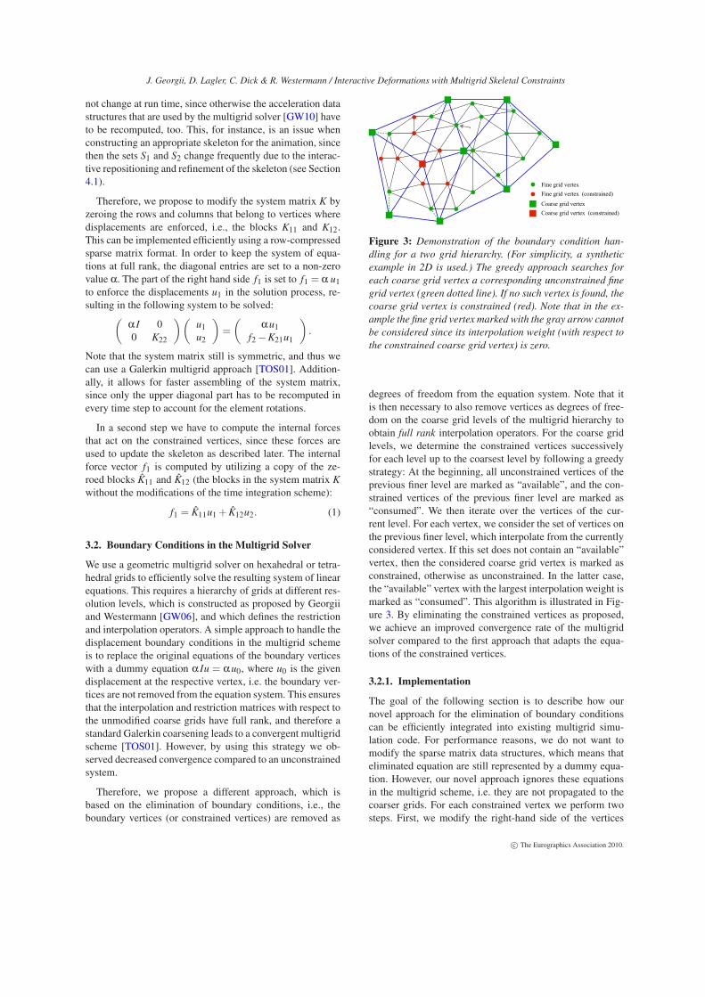
Therefore, we propose a different approach, which isbased on the elimination of boundary conditions, i.e., theboundary vertices (or constrained vertices) are removed as

Figure 3: Demonstration of the boundary condition han-

dling for a two grid hierarchy. (For simplicity, a synthetic

example in 2D is used.) The greedy approach searches for

each coarse grid vertex a corresponding unconstrained fine

grid vertex (green dotted line). If no such vertex is found, the

coarse grid vertex is constrained (red). Note that in the ex-

ample the fine grid vertex marked with the gray arrow cannot

be considered since its interpolation weight (with respect to

the constrained coarse grid vertex) is zero.

degrees of freedom from the equation system. Note that itis then necessary to also remove vertices as degrees of free-dom on the coarse grid levels of the multigrid hierarchy toobtain full rank interpolation operators. For the coarse gridlevels, we determine the constrained vertices successivelyfor each level up to the coarsest level by following a greedystrategy: At the beginning, all unconstrained vertices of theprevious finer level are marked as “available”, and the con-strained vertices of the previous finer level are marked as“consumed”. We then iterate over the vertices of the cur-rent level. For each vertex, we consider the set of vertices onthe previous finer level, which interpolate from the currentlyconsidered vertex. If this set does not contain an “available”vertex, then the considered coarse grid vertex is marked asconstrained, otherwise as unconstrained. In the latter case,the “available” vertex with the largest interpolation weight ismarked as “consumed”. This algorithm is illustrated in Fig-ure 3. By eliminating the constrained vertices as proposed,we achieve an improved convergence rate of the multigridsolver compared to the first approach that adapts the equa-tions of the constrained vertices.

3.2.1. Implementation

The goal of the following section is to describe how ournovel approach for the elimination of boundary conditionscan be efficiently integrated into existing multigrid simu-lation code. For performance reasons, we do not want tomodify the sparse matrix data structures, which means thateliminated equation are still represented by a dummy equa-tion. However, our novel approach ignores these equationsin the multigrid scheme, i.e. they are not propagated to thecoarser grids. For each constrained vertex we perform twosteps. First, we modify the right-hand side of the vertices



in the 1-ring neighborhood to account for the displacementboundary condition (see Section 3.1). Second, we eliminatethe equation at the constrained vertex by zeroing the respec-tive row and column of the matrix (and keeping a diagonalentry).

In principle, we then want to ignore this eliminated equa-tions on the coarser grids, too, which means that we haveto adapt the restriction and interpolation operators in sucha way that eliminated equations do not modify other coarsegrid equations. That is, for the constrained vertices we zerothe respective column in the restriction matrix and the re-spective row in the interpolation matrix.

However, then it might happen that as a result the restric-tion/interpolation matrices do not have full rank. Intuitively,one can see this fact as having more degrees of freedom onthe coarser level than on the finer level, since degrees of free-doms on the finer level are restricted by the boundary con-ditions. In this situation, it is necessary to mark a reasonablenumber of coarse grid vertices as constrained, too, since oth-erwise the coarse grid operator becomes singular. We ensurethis in a further step using our greedy approach as describedabove.

If we have marked a coarse grid vertex as constrained asresult of the greedy approach, we have to ensure that thiscoarse grid vertex gets a dummy equation, too (since other-wise the coarse grid operator will be rank deficient). There-fore, we choose an arbitrary constrained fine grid vertex andmanipulate the restriction/interpolation matrix such that thefine grid (dummy) equation is propagated to the constrainedcoarse grid vertex. In principle, this is the same as eliminat-ing the coarse grid vertex.

The benefit of this procedure is that we neither have tomodify the matrix data structure nor the multigrid code tomanually ignore the constrained vertices in the solution pro-cess. However, the approach has to manipulate the stream ac-celeration data structures [GW10] that is used by the multi-grid solver to efficiently determine the system equations onthe coarser grids. These coarse grid matrices are built bymeans of sparse matrix products involving the interpolationand restriction operators, which are derived from the geo-metric grid hierarchy. To efficiently compute the sparse ma-trix products we use a stream-like layout of a data structurethat allows one to perform these operations in a very cache-efficient way. To incorporate the novel boundary conditionhandling into the optimized multigrid method, we have toupdate the stream data structure, since it embeds respectiveentries of the interpolation and restriction operators for per-formance reasons. Fortunately, this is easily possible sincethe stream layout does not change (the matrix data structuresdo not change), and thus we can easily update the respectiveentries of the interpolation and restriction operators.

4. Skeleton-based Deformation

To enable the described two-way coupling between a skele-ton and a finite element mesh, we now describe the skele-ton construction and the binding of the constructed skele-ton to the mesh. Ideally, one would assume the finite ele-ment mesh vertices to lie on the skeleton’s bone segmentsto properly couple the skeleton simulation with the finite el-ement method as suggested by Capell et al. [CGC∗02a]. Inthis case, however, the finite element mesh has to be adaptedwhenever the skeleton changes, thus prohibiting an interac-tive modification of the skeleton. To overcome this limita-tion, we provide a method to bind a skeleton to a finite el-ement model that does not need to have any vertices on theskeleton.

4.1. Skeleton Editor

Skeleton construction and modification is performed inter-actively via a skeleton editor illustrated in Figure 4. The ed-itor provides the possibility to define different joint types,i.e. either a hinge joint or a ball joint. Furthermore, the usercan add joint limits such as minimal and maximal rotationangle in case of hinge joints, or a cone that defines the pos-sible movements in case of ball joints. These constraints areensured by an inverse kinematic module that is used to de-termine the skeleton’s pose.

Figure 4: A screenshot of the skeleton editor.

4.2. Skeleton Binding

To bind the skeleton to the finite element simulation mesh,we apply the following simple approach: Firstly, we deter-mine for every skeleton bone B j the set of finite elementsit intersects with. From these element set, we consider allelement vertices vi within a predefined distance to the boneB j and project them onto the bone B j to determine a linearinterpolation weight

wi j =(vi −B0

j)T (B1

j −B0j)

‖B1j −B0

j‖2

,

where B0j and B1

j denote the position of the start and endjoints of B j, respectively. If wi j /∈ [0,1], the vertex is not



bound to B j . Otherwise, the weight wi j is stored at the ver-tex together with the respective bone identifier. We will callthese vertices the skeleton vertices in the following. In casea single vertex gets bound to several bones, we consider onlythe closest bone.

The linear interpolation weight is used to transfer move-ments from the skeleton to the finite element mesh. Skeletonvertices are handled as displacement boundary conditions inthe simulation as described above, and the displacements forthese vertices are determined by linearly interpolating thedisplacements of the respective joints using the weights wi j.However, this simple approach has the drawback that it doesnot account for rotations around the bone axis, which canlead to artifacts in the simulation. To avoid this, one can ei-ther generate a mesh which is aligned with the skeleton, i.e.all skeleton vertices lie on the bone segments, or one canadditionally rotate the skeleton vertices around the bone (inwhich case the rotation has to be included as degree of free-dom in the skeleton simulation.)

Additionally, for each bone joint we accumulate the massof the soft body that is relevant for this joint. For each ver-tex i of the finite element model, we first determine its massby gathering the masses of the incident elements, and wethen accumulate this mass to the best-fitting skeleton boneby choosing the closest bone j that satisfies wi j ∈ [0,1]. Fi-nally, the vertex mass is accumulated to the respective startand end joint of the bone j using the respective weights.These joint masses are used to move the skeleton based onforces acting on the skeleton as described in the next sec-tion. It is worth noting that the joint mass is only a roughapproximation, i.e. not all finite element vertices propagatetheir mass since it might happen that there does not exist ajoint with corresponding weight wi j ∈ [0,1]. However, weobserve that this approach effectively increases the stabilityof the proposed two-way coupling, which we describe in thenext section.

4.3. Skeletal Constraints

In the Section 3.1 we have shown how to apply displace-ment boundary conditions to the skeleton vertices of the fi-nite element mesh by fixating these vertices on the skeleton.To let the skeleton being moved by the soft body, we pro-ceed in two steps: Firstly, the forces exerted at the skeletonvertices are determined using the finite element simulation(see Equation 1). Secondly, these forces are accumulated atthe joints of the skeleton by considering the interpolationweights stored at each skeleton vertex. Finally, from the ac-cumulated mass of the soft body at the skeleton’s joints andthe forces acting on it we obtain an update of the position ofthe skeleton’s joint using an Verlet time integration scheme.Since we consider the mass of the deformable body to up-date the skeletal pose, we add inertia to the movement ofthe skeleton, which results in damping of our coupled sim-ulations. To allow for an intuitive control of the amount of

damping, we use a globally defined damping factor by whichthe forces are scaled.

In general, the new positions of the skeleton’s joints couldbe used to define the new pose of the skeleton. However,since the skeleton itself is subject to a number of constraints(joint type, joint limits), we use inverse kinematics to recom-pute the skeleton’s pose. Therefore, the goal position of ev-ery joint is set to the new position computed by the forceintegration. Then, we apply a Jacobian Transpose approach[Bus09] to compute the new skeleton’s pose taking into ac-count the joint limits. Since we only observe small move-ments of the skeleton from one time step to the next, thisapproach yields reasonable results. Upon convergence of theinverse kinematics computation the displacement boundaryconditions of all skeleton vertices are updated with respectto the new skeleton pose. Then, the simulation starts overtaking into account the new boundary conditions.

5. Results

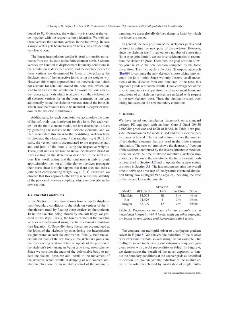
We have tested our simulation framework on a standarddesktop PC equipped with an Intel Core 2 Quad Q94502.66 GHz processor and 8 GB of RAM. In Table 1 we pro-vide information on the models used and the respective per-formance achieved. The second column shows the numberof tetrahedral elements that are used in the finite elementsimulation. The next column shows the degrees of freedomof the skeleton (computed by the inverse kinematic module).Then, we show the time it takes to initialize a skeleton sim-ulation, i.e. to bound the skeleton to the finite element meshas described in Section 4.2 and to update the system matrixas shown in Section 3.1. The last column contains the overalltime to solve one time step of the dynamic corotated simula-tion (using two multigrid V(2,1)-cycles) including the timeof the inverse kinematic module.

Skeleton InitModel #Elements DoFs Skeleton Solve

Manikin 14,062 10 1ms 49msBar 24,576 4 2ms 56ms

Dragon 67,309 12 4ms 203ms

Table 1: Performance Analysis. The bar example uses a

nested grid hierarchy with 4 levels, while the other examples

are based on non-nested grid hierarchies with 3 levels.

We compare our multigrid solver to a conjugate gradientsolver in Figure 5. We analyze the reduction of the relativeerror over time for both solvers using the bar example. Ourmultigrid solver (red) clearly outperforms a conjugate gra-dient solver with Jacobi preconditioner (blue). In Figure 6,we demonstrate the benefit of the novel approach to han-dle the boundary conditions at the coarser grids as describedin Section 3.2. We analyze the reduction of the relative er-ror of the solution achieved by an iteration of single multi-



1e-141e-131e-121e-111e-101e-91e-81e-71e-61e-51e-41e-31e-21e-11e0

0 0.25 0.5 0.75 1 1.25 1.5

Res

idua

l red

ucti

on ||

r k|| 2

/||r 0

|| 2

Time (s)

Solver comparison: Bar, 24K elements

MGCG-Jacobi


0 1 2 3 4 5 6 7 8 9 10 11 12 13 14 15 16

Res

idua

l red

ucti

on ||

r k|| 2

/||r 0

|| 2

Time (s)


MGCG-Jacobi


0 20 40 60 80 100 120 140 160 180 200 220 240 260

Res

idua

l red

ucti

on ||

r k|| 2

/||r 0

|| 2

Time (s)


MGCG-Jacobi

Figure 5: Computational efficiency of different numerical solvers. Our multigrid approach (red) clearly outperforms a conju-

gate gradient solver with Jacobi preconditioner (blue).

grid V(1,1)-cycles with one pre- and post-smoothing Gauss-Seidel step. It can be seen that our approach (“EliminatedBoundary Conditions”) significantly improves the conver-gence rate of the multigrid solver compared to the simpleapproach (“Adapted Equations”). It is worth noting, how-ever, that the latter one shows the same convergence rate asour approach if there are no constrained coarse grid vertices(since the interpolation with eliminated boundary conditionsstill has full rank). One of the main benefits of our approachto eliminate the boundary conditions is that we can improvethe convergence rate without increasing the computationalcosts of a V-cycle.

We allow two different kinds of interaction modes in ourimplementation. Firstly, we can pick joints of the skele-ton and move them to a specific position, which directlydefines the goal positions for the inverse kinematic mod-ule. This mode can be used to directly control the skeletal


0 25 50 75 100 125 150 175 200

Res

idua

l red

ucti

on ||

r k|| 2

/||r 0

|| 2

Number of V-cycles

Multigrid convergence: Bar, 198K elements

MG, eliminated BCMG, adapted equations

Figure 6: Convergence analysis of the multigrid approach

with boundary conditions (bar example). The new approach

to eliminate the boundary conditions on the coarser grids

(red) effectively improves the convergence rate compared

to a standard Galerkin approach with adapted equations

(green).

pose. Secondly, we provide the proposed indirect deforma-tion mode, where the user induces external forces on the ob-ject by mouse movements. The skeleton pose is then auto-matically recomputed as described in Section 4.3. Figure 7shows some results achieved with our approach.

6. Conclusion

We have demonstrated a novel approach to handle skeletalconstraints in deformable object simulations. By using aninverse kinematic approach, we can update the pose of theskeleton, which then determines the boundary conditions inthe finite element simulation. We provide a feedback mode,such that the internal forces acting on the skeleton can beused to automatically update the skeleton.

Moreover, we have shown how to efficiently embed theskeletal constraints into a geometric multigrid approach forthe deformable object simulation. We proposed a novel ap-proach to eliminate the constrained vertices while at thesame time ensuring that the interpolation operator has fullrank. This approach is a general means to handle boundaryconditions in geometric multigrid techniques, for instanceto fixate single vertices. By means of our approach, we canachieve interactive update rates for the simulation of largedeformable bodies with skeletal constraints.

References

[ACP02] ALLEN B., CURLESS B., POPOVIC Z.: Articulatedbody deformation from range scan data. In Proc. of SIGGRAPH

’02 (2002), ACM, pp. 612–619.

[Bar96] BARAFF D.: Linear-time dynamics using lagrange mul-tipliers. In SIGGRAPH ’96: Proceedings of the 23rd annual con-

ference on Computer graphics and interactive techniques (NewYork, NY, USA, 1996), ACM, pp. 137–146.

[Ben07] BENDER J.: Impulse-based dynamic simulation in lineartime. Journal of Computer Animation and Virtual Worlds 18, 4-5(2007), 225–233.

[BFA02] BRIDSON R., FEDKIW R., ANDERSON J.: Robust treat-ment of collisions, contact and friction for cloth animation. InProceedings of SIGGRAPH (2002), pp. 594–603.



Figure 7: A sequence of different skeletal constrained deformations of a manikin. We use a high-resolution render surface as

proposed in [GW05].

[BFGS03] BOLZ J., FARMER I., GRINSPUN E., SCHRÖODER P.:Sparse matrix solvers on the gpu: conjugate gradients and multi-grid. In Proceedings of SIGGRAPH (2003), pp. 917–924.

[BNC96] BRO-NIELSEN M., COTIN S.: Real-time volumet-ric deformable models for surgery simulation using finite ele-ments and condensation. In Proceedings of Eurographics (1996),pp. 57–66.

[Bra77] BRANDT A.: Multi-level adaptive solutions to boundary-value problems. Mathematics of Computation 31, 138 (1977),333–390.

[Bus09] BUSS S. R.: Introduction to inverse kinematics with ja-

cobian transpose, pseudoinverse and damped least squares meth-

ods. Tech. rep., University of California, 2009.

[CBC∗05] CAPELL S., BURKHART M., CURLESS B.,DUCHAMP T., POPOVIC Z.: Physically based rigging fordeformable characters. In Proceedings of the 2005 ACM

SIGGRAPH/Eurographics symposium on Computer animation

(2005), ACM, pp. 301–310.

[CGC∗02a] CAPELL S., GREEN S., CURLESS B., DUCHAMP

T., POPOVIC Z.: Interactive skeleton-driven dynamic deforma-tions. In Proceedings of SIGGRAPH (2002), pp. 586–593.

[CGC∗02b] CAPELL S., GREEN S., CURLESS B., DUCHAMP

T., POPOVIC Z.: A multiresolution framework for dy-namic deformations. In Proceedings of the ACM SIG-

GRAPH/Eurographics Symposium on Computer Animation

(2002), pp. 41–47.

[DDCB01] DEBUNNE G., DESBRUN M., CANI M.-P., BARR

A. H.: Dynamic real-time deformations using space & timeadaptive sampling. In Proceedings of SIGGRAPH (2001),pp. 31–36.

[DGBW08] DICK C., GEORGII J., BURGKART R., WESTER-MANN R.: Computational steering for patient-specific implantplanning in orthopedics. In Proceedings of Visual Computing for

Biomedicine 2008 (2008), pp. 83–92.

[FvdPT01] FALOUTSOS P., VAN DE PANNE M., TERZOPOULOS

D.: Composable controllers for physics-based character anima-tion. In Proceedings of SIGGRAPH ’01 (2001), pp. 251 – 260.

[GKS02] GRINSPUN E., KRYSL P., SCHRÖDER P.: CHARMS:

a simple framework for adaptive simulation. In Proceeding of

SIGGRAPH (2002), pp. 281–290.

[GOT∗07] GALOPPO N., OTADUY M. A., TEKIN S., GROSS

M. H., LIN M. C.: Soft articulated characters with fast contacthandling. Comput. Graph. Forum 26, 3 (2007), 243–253.

[GTT89] GOURRET J.-P., THALMANN N. M., THALMANN D.:Simulation of object and human skin formations in a graspingtask. SIGGRAPH Comput. Graph. 23, 3 (1989), 21–30.

[GW05] GEORGII J., WESTERMANN R.: Interactive Simulationand Rendering of Heterogeneous Deformable Bodies. In Pro-

ceedings of Vision, Modeling and Visualization (2005), pp. 383–390.

[GW06] GEORGII J., WESTERMANN R.: A Multigrid Frame-work for Real-Time Simulation of Deformable Bodies. Com-

puter & Graphics 30 (2006), 408–415.

[GW08] GEORGII J., WESTERMANN R.: Corotated finite ele-ments made fast and stable. In Proc. of the 5th Workshop On Vir-

tual Reality Interaction and Physical Simulation (2008), pp. 11–19.

[GW10] GEORGII J., WESTERMANN R.: A streaming approachfor sparse matrix products and its application in Galerkin multi-grid methods. Electronic Transactions on Numerical Analysis, to

appear (2010).

[HS04] HAUTH M., STRASSER W.: Corotational simulation ofdeformable solids. In Proceedings of WSCG (2004), pp. 137–145.

[HWBO95] HODGINS J. K., WOOTEN W. L., BROGAN D. C.,O’BRIEN J. F.: Animating human athletics. In SIGGRAPH

’95: Proceedings of the 22nd annual conference on Computer

graphics and interactive techniques (New York, NY, USA, 1995),ACM, pp. 71–78.

[IC87] ISAACS P. M., COHEN M. F.: Controlling dynamic sim-ulation with kinematic constraints. SIGGRAPH Comput. Graph.

21, 4 (1987), 215–224.

[JP99] JAMES D. L., PAI D. K.: ArtDefo: accurate real time de-formable objects. In Proceedings of SIGGRAPH (1999), pp. 65–72.



[JZvdP∗08] JU T., ZHOU Q.-Y., VAN DE PANNE M., COHEN-OR D., NEUMANN U.: Reusable skinning templates using cage-based deformations. In Proc. of SIGGRAPH Asia ’08 (2008),ACM, pp. 1–10.

[KH08] KAZHDAN M., HOPPE H.: Streaming multigrid forgradient-domain operations on large images. ACM Trans. Graph.

27, 3 (2008), 1–10.

[MDM∗02] MÜLLER M., DORSEY J., MCMILLAN L., JAGNOW

R., CUTLER B.: Stable real-time deformations. In Proceedings

of ACM SIGGRAPH/Eurographics Symposium on Computer An-

imation (2002), pp. 49–54.

[MG04] MÜLLER M., GROSS M.: Interactive virtual materials.In Proceedings of Graphics Interface (2004), pp. 239–246.

[MHTG05] MÜLLER M., HEIDELBERGER B., TESCHNER M.,GROSS M.: Meshless deformations based on shape matching.ACM Trans. Graph. 24, 3 (2005), 471–478.

[MKN∗04] MÜLLER M., KEISER R., NEALEN A., PAULY M.,GROSS M., ALEXA M.: Point based animation of elas-tic, plastic and melting objects. In Proceedings of the ACM

SIGGRAPH/Eurographics Symposium on Computer Animation

(2004), pp. 141–151.

[Mül08] MÜLLER M.: Hierarchical position based dynamics. InProc. of the 5th Workshop On Virtual Reality Interaction and

Physical Simulation (2008).

[NKJF09] NESME M., KRY P. G., JERÁBKOVÁ L., FAURE F.:Preserving topology and elasticity for embedded deformablemodels. In SIGGRAPH ’09: ACM SIGGRAPH 2009 papers

(New York, NY, USA, 2009), ACM, pp. 1–9.

[NMK∗05] NEALEN A., MÜLLER M., KEISER R., BOXERMAN

E., CARLSON M.: Physically based deformable models in com-puter graphics. In Proceedings of Eurographics (2005), pp. 71–94.

[SF98] SINGH K., FIUME E.: Wires: a geometric deformationtechnique. In Proc. of SIGGRAPH ’98 (1998), ACM, pp. 405–414.

[SPCM97] SCHEEPERS F., PARENT R. E., CARLSON W. E.,MAY S. F.: Anatomy-based modeling of the human muscula-ture. In Proc. of SIGGRAPH ’97 (1997), ACM, pp. 163–172.

[SSF08] SHINAR T., SCHROEDER C., FEDKIW R.: Two-waycoupling of rigid and deformable bodies. In Proc. of the 2008

ACM SIGGRAPH/Eurographics Symposium on Computer Ani-

mation (2008), Eurographics Association, pp. 95–103.

[SYBF06] SHI L., YU Y., BELL N., FENG W.-W.: A fast multi-grid algorithm for mesh deformation. ACM Trans. Graph. 25, 3(2006), 1108–1117.

[SZHB06] SONG C., ZHANG H.-X., HUANG J., BAO H.-J.:Meshless simulation for skeleton driven elastic deformation.Journal of Zhejiang University - Science A 7 (2006), 1596–1602.

[TF88] TERZOPOULOS D., FLEISCHER K.: Modeling inelasticdeformation: Viscoelasticity, plasticity, fracture. In Proceedings

of SIGGRAPH (1988), pp. 269–278.

[TOS01] TROTTENBERG U., OOSTERLEE C., SCHÜLLER A.:Multigrid. Academic Press, 2001.

[TPBF87] TERZOPOULOS D., PLATT J., BARR A., FLEISCHER

K.: Elastically deformable models. In Proceedings of SIG-

GRAPH (1987), pp. 205–214.

[WDGT01] WU X., DOWNES M. S., GOKTEKIN T., TENDICK

F.: Adaptive nonlinear finite elements for deformable body sim-ulation using dynamic progressive meshes. In Proceedings of

Eurographics (2001), pp. 349–358.

[WGF08] WEINSTEIN R., GUENDELMAN E., FEDKIW R.:Impulse-based control of joints and muscles. IEEE Transactions

on Visualization and Computer Graphics 14, 1 (2008), 37–46.

[WT04] WU X., TENDICK F.: Multigrid integration for interac-tive deformable body simulation. In Proceedings of International

Symposium on Medical Simulation (2004), pp. 92–104.

[WTF06] WEINSTEIN R., TERAN J., FEDKIW R.: Dynamicsimulation of articulated rigid bodies with contact and collision.IEEE Transactions on Visualization and Computer Graphics 12,3 (2006), 365–374.

[WVG97] WILHELMS J., VAN GELDER A.: Anatomically basedmodeling. In Proc. of SIGGRAPH ’97 (1997), ACM, pp. 173–180.

[ZSTB10] ZHU Y., SIFAKIS E., TERAN J., BRANDT A.: Anefficient multigrid method for the simulation of high-resolutionelastic solids. ACM Trans. Graph. 29, 2 (2010), 1–18.


interactive deformations with multigrid skeletal … · interactive deformations with multigrid...

Documents