interactive image segmentation using an adaptive gmmrf model€¦ · interactive segmentation by...

Interactive Image Segmentation using an adaptiveGMMRF model

A. Blake, C. Rother, M. Brown, P. Perez, and P. Torr

Microsoft Research Cambridge UK,7 JJ Thomson Avenue, Cambridge CB3 0FB, UK.

http://www.research.microsoft.com/vision/cambridge

Abstract. The problem of interactive foreground/background segmentation instill images is of great practical importance in image editing. The state of the artin interactive segmentation is probably represented by the graph cut algorithm ofBoykov and Jolly (ICCV 2001). Its underlying model uses both colour and con-trast information, together with a strong prior for region coherence. Estimationis performed by solving a graph cut problem for which very efficient algorithmshave recently been developed. However the model depends on parameters whichmust be set by hand and the aim of this work is for those constants to be learnedfrom image data.First, a generative, probabilistic formulation of the model is set out in terms of a“Gaussian Mixture Markov Random Field” (GMMRF). Secondly, a pseudolike-lihood algorithm is derived which jointly learns the colour mixture and coherenceparameters for foreground and background respectively. Error rates for GMMRFsegmentation are calculated throughout using a new image database, available onthe web, with ground truth provided by a human segmenter. The graph cut al-gorithm, using the learned parameters, generates good object-segmentations withlittle interaction. However, pseudolikelihood learning proves to be frail, whichlimits the complexity of usable models, and hence also the achievable error rate.

1 Introduction

The problem of interactive image segmentation is studied here in the framework usedrecently by others [1–3] in which the aim is to separate, with minimal user interaction,a foreground object from its background so that, for practical purposes, it is availablefor pasting into a new context. Some studies [1, 2] focus on inference of transparencyin order to deal with mixed pixels and transparent textures such as hair. Other studies[4, 3] concentrate on capturing the tendency for images of solid objects to be coherent,via Markov Random Field priors such as the Ising model. In this setting, the segmenta-tion is “hard” — transparency is disallowed. Foreground estimates under such modelscan be obtained in a precise way by graph cut, and this can now be performed veryefficiently [5]. This has application to extracting the foreground object intact, even incamouflage — when background and foreground colour distributions overlap at leastin part. We have not come across studies claiming to deal with transparency and cam-ouflage simultaneously, and in our experience this is a very difficult combination. Thispaper therefore addresses the problem of hard segmentation problem in camouflage,and does not deal with the transparency issue.

2 Blake et al.

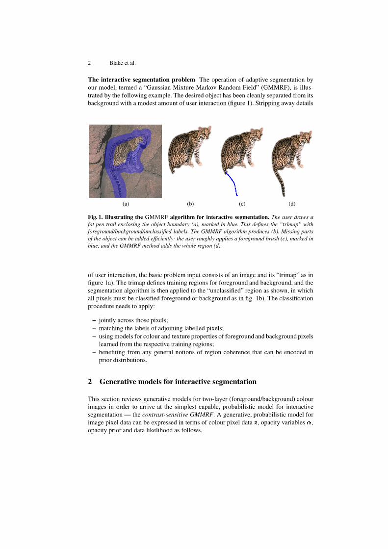
The interactive segmentation problem The operation of adaptive segmentation byour model, termed a “Gaussian Mixture Markov Random Field” (GMMRF), is illus-trated by the following example. The desired object has been cleanly separated from itsbackground with a modest amount of user interaction (figure 1). Stripping away details

(a) (b) (c) (d)

Fig. 1. Illustrating the GMMRF algorithm for interactive segmentation. The user draws afat pen trail enclosing the object boundary (a), marked in blue. This defines the “trimap” withforeground/background/unclassified labels. The GMMRF algorithm produces (b). Missing partsof the object can be added efficiently: the user roughly applies a foreground brush (c), marked inblue, and the GMMRF method adds the whole region (d).

of user interaction, the basic problem input consists of an image and its “trimap” as infigure 1a). The trimap defines training regions for foreground and background, and thesegmentation algorithm is then applied to the “unclassified” region as shown, in whichall pixels must be classified foreground or background as in fig. 1b). The classificationprocedure needs to apply:

– jointly across those pixels;– matching the labels of adjoining labelled pixels;– using models for colour and texture properties of foreground and background pixels

learned from the respective training regions;– benefiting from any general notions of region coherence that can be encoded in

prior distributions.

2 Generative models for interactive segmentation

This section reviews generative models for two-layer (foreground/background) colourimages in order to arrive at the simplest capable, probabilistic model for interactivesegmentation — the contrast-sensitive GMMRF. A generative, probabilistic model forimage pixel data can be expressed in terms of colour pixel data � , opacity variables � ,opacity prior and data likelihood as follows.

Interactive segmentation by GMMRF 3

Image � is an array of colour (RGB) indexed by the (single) index � :�� with corresponding hidden variables for transparency � �� , and hiddenvariables for mixture index � �� !�� "�#�$� . Each pixel is considered, in general,to have been generated as an additive combination of a proportion �%� ( &(' �� '*) )of foreground colour with a proportion )$+ �,� of background colour [2, 1]. Here weconcentrate attention on the hard segmentation problem in which �%�-� & � ) — binaryvalued.

Gibbs energy formulation Now the posterior for � is given by.�� 0/ �1��32�45.�� 6/ �1� (1)

and .�� 6/ �1�%� ).��1� .�� /7� � � �8.�� (2)

This can be written as a Gibbs distribution, omitting the normalising constant )�9 .��1�which is anyway constant with respect to � :.�� 6/ �1�%: );,<>=�?!@$+BADCBE F�G3A �IH(JLKMJON% (3)

The intrinsic energies K and N encode the prior distributions:.�� %: =�?!@�+ KQPRTSU.�� V/�� : =�?!@$+ N (4)

and the extrinsic energy H defines the likelihood term.�� /7� � � �%�3W � .�� / ��"�#�X�� );,<Y=�?!@�+ HZ (5)

Simple colour mixture observation likelihood A simple approach to modelling colourobservations is as follows. At each pixel, foreground colour is considered to be gener-ated randomly from one of [ Gaussian mixture components with mean \ �] � � � andcovariance ^ �] � � � from the foreground, and likewise for the background:.�� / ��_�"�#�X�%�U`a��Tb \ � �#��X�� ^ � ��T�c��d��e� & � ) ��#�f� ) �� [ (6)

and the components have prior probabilities.�� / � ��gW � .�� #� / ��X� CBE F�G .�� #� / ��T�%�ih%� �#�_��X�� (7)

The exponential coefficient for each component, referred to here as the “extrinsic energycoefficient” is denoted j � ��k�� l � ^ � ��k�c�"m

. The corresponding extrinsic term inthe Gibbs energy is given by HU�32 �on � (8)

4 Blake et al.CBGX=�p�= n �e��q �� +6\ � �#�_��X�srut j � �#�_��X��q �� +6\ � �#�_��X�sr_ (9)

A useful special case is the isotropic mixture in which j � �v��T�%�gwx� �#�_��X�]y .Note that, for a pixelwise-independent likelihood model as in (6), the partition func-

tion;,<

for the likelihood decomposes multiplicatively across sites � . Since also thepartition function

;,zfor the prior is always independent of � , the MAP estimate of� can be obtained (3) by minimising AU+i{ |#} ;%<

with respect to � and this can beachieved exactly, given that �k� is binary valued here, using a “minimum cut” algorithm[4] which has recently been developed [3] to achieve good segmentation in interactivetime (around 1 second for a ~&#& l

image).

Simple opacity prior (No spatial interaction) The simplest choice of a joint prior.�� is the spatially trivial one, decomposing into a product of marginals.�� %� W � .��X�with, for example, .��k�X� uniform over �k�o�� & � )� (hard opacity) or �k��q & � ) r(variable transparency). This is well known [3] to give poor results and this will bequantified in section 5.

Ising Prior In order to convey a prior on object coherence, .�� can be spatiallycorrelated, for example via a first order Gauss-Markov interaction [6, 7] as, for example,in the Ising prior: .�� : =�?!@$+ K CBE F�G K5�M��2�� v�� q ��(��I� � rs� (10)

where q �Xr denotes the indicator function taking values & � ) for a predicate � , and where�is the set of all cliques in the Markov network, assumed to be two-pixel cliques here.

The constant � is the Ising parameter, determining the strength of spatial interaction.The MAP estimate of � can be obtained by minimising with respect to � the Gibbsenergy (3) with H as before, and the Ising K (10). This can be achieved exactly, giventhat �� is binary valued here, using a “minimum cut” algorithm [4]. In practice [3] thehomogeneous MRF succeeds in enforcing some coherence, as intended, but introduces“Manhattan” artefacts that point to the need for a more subtle form of prior and/or datalikelihood, and again this is quantified in section 5.

3 Incorporating contrast dependence

The Ising prior on opacity, being homogeneous, is a rather blunt instrument, and it isconvincingly argued [3] that a “prior” that encourages object coherence only wherecontrast is low, is far more effective. However, a “prior” that is dependent on data inthis way (dependent on data in that image gradients are computed from intensities � ) is


not strictly a prior. Here we encapsulate the spirit of a contrast-sensitive “prior” moreprecisely as a gradient dependent likelihood term of the form� � �� / � �c�%�]�� (11)

where � is a further coherence parameter in a Gauss-Markov process over � .It turns out that the contrast term introduces a new technical issue in the data-

likelihood model: long-range interactions are induced that fall outside the Markov frame-work, and therefore strictly fall outside the scope of graph cut optimisation. The long-range interaction is manifested in the partition function

;�<for the data likelihood. This

is an inconvenient but inescapable consequence of the probabilistic view of the contrast-sensitive model. While it imperils the graph cut computation of the MAP estimate, andthis will be addressed in due course, correct treatment of the partition function turns outto be critical for adaptivity. This is because of the well-known role of partition func-tions [7] in parameter learning for Gibbs distributions. Note also that recent advancesin Discriminative Random Fields [8] which can often circumvent such issues, turn outnot to be applicable to using the GMMRF model with trimap labelling.

3.1 Gibbs energy for contrast-sensitive GMMRF

A modified Gibbs energy that takes contrast into account is obtained by replacing theterm K in (10) by K��L��2�� v�� q ��(��i� � r =�?!@$+ �� + �� l � (12)

which relaxes the tendency to coherence where image contrast is strong. The constant� is supposed to relate to � via observation noise and we set�� g�L� � � � + �� l�� CBE F�G �0�M� (13)

where � � � � denotes expectation over the test image sample, and taking the constant�5�i� is justified later.The results of minimising A ��HIJDK � (neglecting { |#} ;,<

— see later) givesconsiderably improved segmentation performance [3]. In our experience “Manhattan”artefacts are suppressed by the reduced tendency of segmentation boundaries to followManhattan geodesics, in favour of following lines of high contrast. Results in section 5will confirm quantitatively the performance gain.

3.2 Probabilistic model

In the contrast-sensitive version of the Gibbs energy, the term K � no longer correspondsto a prior for � , as it did in the homogeneous case (10). The entire Gibbs energy is nowA �32 ��n �$JV��2�� v�� q ��-��I� � r =�?!@$+ �� + �� l (14)

6 Blake et al.

Adding a “constant” term ��2�� v�� )B+6=�?!@$+ �� + �� l � (15)

to A has no effect on the minimum of A ��k� w.r.t. � , and transforms the problem in ahelpful way as we will see. The addition of (15) gives A �3K-J�H where K is the earlierIsing prior (10) and now H is given byHU� 2 ��n �$JV� 2�� v�� q ��e�I� � r�� )B+6=�?!@$+ ��#�� + �� l �� (16)

with separate texture constants � z �c�_ for foreground and background respectively. Thisis a fully generative, probabilistic account of the contrast-sensitive model, cleanly sep-arating prior and likelihood terms. Transforming A by the addition of the constant term(15) has had several beneficial effects. First it separates the energy into a componentK which is active only at foreground/background region boundaries, and a componentH whose contrast term acts only within region. It is thus clear that the parameter � isa textural parameter — and that is why it makes sense to learn separate parameters� z ��_ . Secondly when, for tractability in learning, the Gibbs energy is approximatedby a quadratic energy in the next section 4, the transformation is in fact essential for theresulting data-likelihood MRF to be proper (ie capable of normalisation).

Inference of foreground and background labels from posterior Given that H isnow dependent on � and � simultaneously, the partition function

; <for the likelihood,

which was a locally factorised function for the simple likelihood model of section 2,now contains non-local interactions over � . It is no longer strictly correct that the pos-terior can be maximised simply by minimising A �¡HUJ3K . Neglecting the partitionfunction

;,<in this way can be justified, it turns out, by a combination of experiment

and theory — see section 6.MAP inference of � is therefore done by applying min cut as in [3] to the Gibbs

energy A . For this step we can either marginalise over � , or maximize with respect to� , the latter being computationally cheaper and tending to produce very similar resultsin practice.

4 Learning parameters

This section addresses the critical issue of how mixture parameters \ � ��k� , ^ � ��k�and h%� ��k� can be learned from data simultaneously with coherence parameters �7�x� � .In the simple uncoupled model with �_�� & for �¡� & � ) mixture parameters canbe learned by conventional methods, but when coherence parameters are switched on,learning of all parameters is coupled non-trivially.


4.1 Quadratic approximation

It would appear that the exponential form of H in (16) is an obstacle to tractability ofparameter learning, and so the question arises whether it is an essential component ofthe model. Intuitively it seems well chosen because of the switching behaviour built intothe exponential, that switches the model in and out of its “coherent” mode. Nonetheless,in the interests of tractability we use a quadratic approximation, solely for the parameterlearning procedure. The approximated form of the extrinsic energy (16) becomes:H£¢Z� 2 �on �$J 2�� v�� #�_q ��e�I� � r � � � + �� l (17)

and the approximation is good provided ��#� � � � + �� l�¤ � .

Learning ¥ Note that since the labelled data consists typically of separate sets offoreground and background pixels respectively (fig 1a,b) there is no training data con-taining the boundary between foreground and background. There is therefore no dataover which the Ising term (10) can be observed, since � no longer appears in the ap-proximated H ¢ . Therefore � cannot simply be learned from training data in this versionof the interactive segmentation problem. However for the switching of the exponentialterm in (16) to act correctly it is clear that we must have=�?!@$+ ��#�� + �� l�¦ ) (18)

throughout regions of homogeneous texture so, over background for instance, we musthave �(§O��#� � � � + �� l , which is also the condition for good quadratic approximationabove. Given that the statistics of � � + �� are found to be consistently Gaussian inpractice, this is secured by (13).

4.2 Pseudolikelihood

A well established technique for parameter estimation in formally intractable MRFs likethis one is to introduce a “pseudolikelihood function” [6] and maximise it with respectto its parameters. The pseudolikelihood function has the form¨ � =�?!@$+BA ¢ (19)

where A ¢ will be called the “pseudo-energy”, and note that¨

is free of any partitionfunction. There is no claim that

¨itself approximates the true likelihood, but that, under

certain circumstances, its maximum coincides asymptotically with that of the likelihood[7] — asymptotically, that is, as the size of the data � tends to infinity. Strictly the resultsapply for integer-valued MRFs, so formally we should consider � to be integer-valued,and after all it does represent a set of quantised colour values.

Following [7], the pseudo-energy is defined to beA ¢Z�32 � � +�{ |#} .�� / �#�� c� (20)

8 Blake et al.

where �#�e�I�v©1�� — the entire data array omitting �� . Now.�� / �#� � � � ��V.�� / �� ª��Y«%� � � � � � � (21)

by the Markov property, where «�� is the “Markov blanket” at grid point � — the setof its neighbours in the Markov model. For the earlier example of a first-order MRF,«%� simply contains the N, S, E, W neighbours of � . Taking into account the earlierdetails of the probability distribution over the Markov structure, it is straightforward tobe show that, over the training set.�� / �� xª��«%� � � � � � �%: =�?!@$+o¬ n �$J 2� �#v� NT� �B® (22)

where NT� � �M��#�_q � � �i��vr � �� + � � � l (23)

Terms �,q � � ��¯��1r from K have been omitted since they do not occur in the trainingsets of the type used here (fig 1), as mentioned before. Finally, the pseudo-likelihoodenergy function A ¢ �32 � A ¢� CBE F�G3A ¢� � ; ¢� J n �$J°2� �#v� NT� � (24)

and =�?!@�+ ; ¢� is the (local) partition function.

4.3 Parameter estimation by autoregression over the pseudolikelihood

It is well known that the parameters of a Gaussian MRF can be obtained from pseu-dolikelihood as an auto-regression estimate [9]. For tractability, we split the estimationproblem up into ±[ problems, one for each foreground and background mixture com-ponent, treated independently except for sharing common constants � z

and �_ . For thispurpose, the mixture index �1� at each pixel is determined simply by maximisation ofthe local likelihood: �#�f�iP p�}%² P ?³ .�� / ��"�X��h �#�³ (25)

Further, for tractability, we restrict the data �� to those pixels (much the majority inpractice) whose foreground/background label � agrees with all its neighbours — ie the� for which � � �I��´ |#p P { { ª��Y«%�� Observables �� with a given class label �k� and component index �1� are then dealt withtogether, in accordance with the pseudolikelihood model above, as variables from theregression �� + � / �#�fµ�`0��¶��u·¸� + �1�� ^ � (26)

where ·¸�f� )¹ 2� �#v� � � � (27)


and¹ � / «%� / . The mean colour is estimated simply as�� v� (28)

where � � � � denotes the sample mean over pixels from class � and with componentindex � . We can solve for ¶ and ^ using standard linear regression as follows:¶g� � �� + �1��u· + �1� t �Bº � �u· + �1��u· + �v� t ��» m

(29)

and ^ �0��¼"¼�t � CBGX=�p�= ¼£�i� + � + ¶��u· + �v�� (30)

Lastly, model parameters for each colour component, for instance of the back-ground, should be obtained to satisfy¹ � z y�� ^ m ¶ (31)j � �#��T�%� ^ m + ¹ � z yT� (32)\ � �#��T�%� �X� (33)

and similarly for the foreground.Note there are some technical problems here. First is that (31) represents a constraint

that is not necessarily satisfied by ^ and ¶ , and so the regression needs to be solvedunder this constraint. Second is that in (32) j � �v�_��X� should be positive definite butthis constraint will not automatically be obeyed by the solution of the autoregression.Thirdly that one value of � z

needs to satisfy the set of equations above for all back-ground components. The first problem is dealt with by restricting j to be isotropic sothat ^ and ¶ must also be isotropic and the entire set of equations are solved straightfor-wardly under isotropy constraints. (In other words, each colour component is regressedindependently of the others.) It turns out that this also solves the second problem. Anunconstrained autoregression on typical natural image data, with general symmetricmatrices for the j � �1�_��X� , will, in our experience, often lead to a non-positive defi-nite solution for j � �1�_��X� and this is unusable in the model. Curiously this problemwith pseudolikelihood and autoregeression seems not to be generally acknowledged instandard texts [7, 9]. Empirically however we have found that the problem ceases withisotropic j � �#��X� , and so we have used this throughout our experiments. The use ofisotropic components seems not to have much effect on quality provided that, of course,a larger number of mixture components must be used than for equivalent performancewith general symmetric component-matrices. Lastly, the tying of � z

across componentscan be achieved simply by averaging post-hoc, or by applying the tying constraint ex-plicitly as part of the regression which is, it turns out, quite tractable (details omitted).

5 Results

Testing of the GMMRF segmentation algorithms uses a database of ~& images. Wecompare the performance of: i) Gaussian colour models, with no spatial interaction; ii)the simple Ising model; iii) the full contrast-sensitive GMMRF model with fixed inter-action parameter � ; iv) the full GMMRF with learned parameters. Results are obtainedusing � -connectivity, and isotropic Gaussian mixtures with [ �I½ & components as thedata potentials n � .

10 Blake et al.

(a) (b) (c)

(d) (e) (f)

Fig. 2. (a,d) Two images from the test database. (b,e) User defined trimap with foreground (white),background (black) and unclassified (grey). (c,f) Expert trimap which classifies pixels into fore-ground (white), background (black) and unknown (grey); unknown here refers to pixels too closeto the object boundary for the expert to classify, including mixed pixels.

Test Database The database contains )�~ training and ½ ~ test images, available on-line1. The database contrasts with the form of ground truth supplied with the Berkeleydatabase2 which is designed to test exhaustive, for bottom up segmentation [10]. Eachimage in our database contains a foreground object in a natural background environ-ment (see fig. 2). Since the purpose of the dataset is to evaluate various algorithms forhard image segmentation, objects with no or little transparency are used. Consequently,partly transparent objects like trees, hair or glass are not included. Two kinds of labeledtrimaps are assigned to each image. The first is the user trimap as in fig. 2(b,e). Thesecond is an “expert trimap” obtained from painstaking tracing of object outlines witha fine pen (fig. 2(c,f)). The fine pen-trail covers possibly mixed pixels on the objectboundary. These pixels are excluded from the error rate measures reported below, sincethere is no definitive ground truth as to whether they are foreground or background.

Evaluation Segmentation error rate is defined as¼£� R | ²¾EÀ¿�Á�{ P ¿�¿cE ÂT= S @XE ?!=�{À¿R | @XE ?!=�{À¿xE R�ÃXR Á�{ P ¿�¿cE ÂT= S p�=�}#E | R � (34)

where “misclassified pixels” excludes those from the unclassified region of the experttrimap. This simple measurement is sufficient for a basic evaluation of segemntation

1 http://www.research.microsoft.com/vision/cambridge/segmentation/2 http://www.cs.berkeley.edu/projects/vision/grouping/segbench/


performance. It might be desirable at some later date to devise a second measure thatquantifies the degree of user effort that would be required to correct errors, for exampleby penalising scattered error pixels.

0 200 4003

4

5

6

γ

Error rate (%)

Fig. 3. The error rate on the training set of Ä�Å images, using different values for Æ . The minimumerror is achieved for Æ¾ÇUÈ7Å . The GMMRF model uses isotropic Gaussians and É -connectivity.

Test database scores In order to compare the GMMRF method with alternative meth-ods, a fixed value of the Ising parameter � is learned discriminatively by optimisingperformance over the training set (fig. 3), giving a value of �d� ±#~ . Then the accompa-nying � constant is fixed as in (13). For full Gaussians and Ê -connectivity the learnedvalue was �M� ±& . The performance on the test set is summarized in figure 4 for the

Segmentation model Error rateGMMRF; discriminatively learned Æ�ÇUÈ�Ë ( Ì¯ÇLÄ�Ë full Gaussian) Í�Î Ï�ÐLearned GMMRF parameters ( ÌDÇUÑ7Ë isotropic Gauss.) ÒÎ Ó %GMMRF; discriminatively learned Æ�ÇUÈ7Å ( Ì¯Ç�Ñ7Ë isotropic Gaussian) ÏÎ É %Strong interaction model ( Æ�ÇLÄ�Ë7Ë7Ë ; Ì¯Ç�Ñ7Ë isotropic Gaussian) Ä7Ä7Î Ë %Ising model ( Æ�ÇUÈ7Å ; Ì¯Ç�Ñ7Ë isotropic Gaussian) Ä7Ä7Î È %Simple mixture model – no interaction ( ÌDÇ�Ñ7Ë isotropic Gaussian) Ä�ÓÎ Ñ %

Fig. 4. Error rates on the test data set for different models and parameter determination regimes.For isotropic Gaussians, the full GMMRF model with learned parameters outperforms both thefull model with discriminatively learned parameters, and simpler alternative models. However,exploiting a full Gaussian mixture model improves results further.

various different models and learning procedures. Results for the two images of figure2 from the test database, are shown in figure 5. As might be expected, models with verystrong spatial interaction, simple Ising interaction, or without any spatial interaction atall, all perform poorly. The model with no spatial interaction has a tendency to generatemany isolated, segmented regions (see fig. 5). A strong interaction model ( �U� )7&#&#& )has the effect of shrinking the the object with respect to the true segmentation. The Isingmodel, with �V� ±#~ set by hand, gives slightly better results, but introduces “Manhat-tan” artefacts — the border of the segmentation often fails to correspond to image edges.The inferiority of the Ising model and the “no interaction model” has been demonstratedpreviously [3] but here is quantified for the first time.

12 Blake et al.

In contrast, the GMMRF model with learned � is clearly superior. For isotropicGaussians and � -connectivity the GMMRF model with parameters learned by the newpseudolikelihood algorithm leads to slightly better results than using the discrimina-tively learned � .

The lowest error rate, however, was achieved using full covariance Gaussians in theGMMRF with discriminatively learned � . We were unable to compare with pseudolike-lihood learning; the potential instability of pseudolikelihood learning (section 4) turnsout to be an overwhelming obstacle when using full covariance Gaussians.

6 Discussion

We have formalised the energy minimization model of Boykov and Jolly [3] for fore-ground/background segmentation as a probabilistic GMMRF and developed a pseudo-likelihood algorithm for parameter learning. A labelled database has been constructedfor this task and evaluations have corroborated and quantified the value of spatial inter-action models — the Ising prior and the contrast-sensitive GMMRF. Further, evaluationhas shown that parameter learning for the GMMRF by pseudolikelihood is effective.Indeed, it is a little more effective than simple discriminative learning for a compara-ble model (isotropic GMMRF); but the frailty of pseudolikelihood learning limits thecomplexity of model that can be used (eg full covariance GMMRF is impractical) andthat in turn limits achievable performance. A number of issues remain for discussion,as follows.

DRF. — the Discriminative Random Field model [8] has recently been shown to bevery effective for image classification tasks. It has the great virtue of banishing theissues concerning the likelihood partition function

;�<that affect the GMMRF. However

it can be shown that the DRF formulation cannot be used with the form of GMMRFdeveloped here, and trimap labelled data, because the parameter learning algorithmbreaks down (details omitted for lack of space).

Line process. The contrast-sensitive GMMRF has some similarity to the well knownline process model [11]. In fact it has an important additional feature, that the observa-tion model is a non-trivial MRF with spatial interaction (the contrast term), and this isa crucial ingredient in the success of contrast-sensitive GMMRF segmentation.

Likelihood partition function. As mentioned in section 3.2, the partition function;,<depends on � and this dependency should be taken into account when searching the

MAP estimate of � . However, for the quadratically approximated extrinsic energy (17),this partition function is proportional to the determinant of a sparse precision matrix,which can be numerically computed for given parameters and � . Within the range ofvalues used in practice for the different parameters, we found experimentally that{ |#} ;,< � � �%� Á�| R ¿]F JOÔa2�� v�� q ��-��I� � rs� (35)

with Ô varying within a range � & � & ~ � . Hence, by ignoring { |#} ;�<in the global energy

to be minimised, we assume implicitly that the prior is effectively Ising with slightly


weaker interaction parameter � + Ô . Since we have seen that graph cut is relativelyinsensitive (fig. 3) to perturbations in � , this justifies neglect of the extrinsic partition fn;,<

and the application of graph cut to the Gibbs energy alone.

Adding parameters to the MRF. It might seem that segmentation performance couldbe improved further by allowing more general MRF models. They would have greaternumbers of parameters, more than could reasonably be set by hand, and this oughtto press home the advantage of the new parameter learning capability. We have runpreliminary experiments with i) spatially anisotropic clique potentials, ii) larger neigh-bourhoods (8-connected) and iii) independent, unpooled foreground and backgroundtexture parameters � z

and �_ (using min cut over a directed graph). However, in allcases error rates were substantially worsened. A detailed analysis of these issues is partof future research.

Acknowledgements. We gratefully acknowledge discussions with and assistance fromP. Anandan, C.M. Bishop, B. Frey, T. Werner, A.L. Yuille and A. Zisserman.

References

1. Chuang, Y.Y., Curless, B., Salesin, D., Szeliski, R.: A Bayesian approach to digital matting.In: Proc. Conf. Computer Vision and Pattern Recognition. (2001) CD–ROM

2. Ruzon, M., Tomasi, C.: Alpha estimation in natural images. In: Proc. Conf. Computer Visionand Pattern Recognition. (2000) 18–25

3. Boykov, Y., Jolly, M.P.: Interactive graph cuts for optimal boundary and region segmentationof objects in N-D images. In: Proc. Int. Conf. on Computer Vision. (2001) CD–ROM

4. Greig, D., Porteous, B., Seheult, A.: Exact MAP estimation for binary images. J. RoyalStatistical Society 51 (1989) 271–279

5. Kolmogorov, V., Zabih, R.: What energy functions can be minimized via graph cuts? IEEETrans. on Pattern Analysis and Machine Intelligence in press (2003)

6. Besag, J.: On the statistical analysis of dirty pictures. J. Roy. Stat. Soc. Lond. B. 48 (1986)259–302

7. Winkler, G.: Image analysis, random fields and dynamic Monte Carlo methods. Springer(1995)

8. Kumar, S., Hebert, M.: Discriminative random fields: A discriminative framework for con-textual interaction in classification. In: Proc. Int. Conf. on Computer Vision. (2003) CD–ROM

9. Descombes, X., Sigelle, M., Preteux, F.: GMRF parameter estimation in a non-stationaryframework by a renormalization technique. IEEE Trans. Image Processing 8 (1999) 490–503

10. Malik, J., Belongie, S., Leung, T., Shi, J.: Contour and texture analysis for image segmenta-tion. Int. J. Computer Vision 43 (2001) 7–27

11. Geman, S., Geman, D.: Stochastic relaxation, Gibbs distributions, and the Bayesian restora-tion of images. IEEE Trans. on Pattern Analysis and Machine Intelligence 6 (1984) 721–741

14 Blake et al.

GMMRF; Æ�ÇUÈ�Ë ; full Gauss. GMMRF; Æ learned GMMRF; Æ�ÇUÈ7ÅÕ�Ö�Ö�×�Ö ÇLÄ7Î Å % Õ�Ö�Ö�×�Ö ÇVÉ#Î Å % Õ�Ö�Ö�×�Ö ÇVÉ#Î Í %

Ising model; Æ�ÇUÈ7Å Strong interaction; Æ¾ÇLÄ�Ë7Ë7Ë No interactionÕ�Ö�Ö�×�Ö ÇUÅ�Î Ï % Õ�Ö�Ö�×�Ö ÇUÍ�Î Ó % Õ�Ö�Ö�×�Ö Ç�ÒÎ Ï %

GMMRF; Æ�ÇUÈ�Ë ; full Gauss. GMMRF; Æ learned GMMRF; Æ�ÇUÈ7ÅÕ�Ö�Ö�×�Ö Ç�ÓÎ Ò % Õ�Ö�Ö�×�Ö ÇUÍ�Î Ë % Õ�Ö�Ö�×�Ö Ç�ÏÎ Í %

Ising model; Æ�ÇUÈ7Å Strong interaction; Æ¾ÇLÄ�Ë7Ë7Ë No interactionÕ�Ö�Ö�×�Ö ÇLÄ�ËÎ Í % Õ�Ö�Ö�×�Ö ÇLÄ�Å�Î Ï % Õ�Ö�Ö�×�Ö ÇUÈ�ËÎ Ë %

Fig. 5. Results for various segmentation algorithms (see fig. 4) for the two images shown in fig.2. For both examples, the error rate increases from top left to bottom right. GMMRF with pseu-dolikelihood learning outperforms the GMMRF with discriminatively learned Æ parameters, andthe various simpler alternative models. The best result is achieved however using full covarianceGaussians and discriminatively learned Æ .

interactive image segmentation using an adaptive gmmrf model€¦ · interactive segmentation by...

Documents