intercepting modern signals - ieee well as low power long duration signals are present • today’s...

The Future of EW and Modern Radar Signals

Richard G. WileyResearch Associates of Syracuse, Inc.

6780 Northern Blvd., E. Syracuse, NY 13057315-463-2266 [email protected]

The Signal Environment

• The period since WWII has seen the deployment of large number of pulsed radars, seekers and other threat systems in the microwave bands

• Recently newer, high duty factor or CW systems have been deployed.

• The reduction in peak power makes EW more difficult (but not impossible)

Tomorrow’s Threats plus Yesterday’s and Today’s

• There is a trend to long duration, low peak power signals to make them less vulnerable

• But older systems will still be used, too.• Therefore EW systems must operate when

both the high power, short duration signals as well as low power long duration signals are present

• Today’s EW Receivers are optimized for Yesterday’s Threat Environment

Modern Signals are Different

• “LPI” Radars are being deployed which use long duration pulses and pulse compression

• The next generation of EW equipment must be able to cope with these threats

Low probability of ID

• The threat recognition process can clearly be disrupted by transmitting unexpected parameters.

• Using parameters similar to another non-threatening radar is one example

• Introducing parameter agility is another• These will probably deceive the opponent

only for a short time

Low Probability of Interception• Another is to try to make the signal so weak

that the ESM system cannot detect it. • As we will see, for radar this can be

difficult. It is this aspect that we will spend most of our time examining

• Spread Spectrum is a term used in communications. (I say it does not apply to radar!)

Radar is not “Spread Spectrum”• In communications, the transmitted spectrum is

spread over an arbitrarily wide band. The spreading is removed in the receiver. The interceptor may not be able to detect the wideband signal in noise.

• In radar, the transmitted bandwidth determines range resolution. Wideband signals break up the echo and thus reduce target detectability– what you transmit is what you get back– synchronizing the receiver is the ranging process

Modern Radar Waveforms

• Energy on target, not peak power determines radar performance

• A CW radar has peak power 30 dB lower than a pulsed radar with a duty factor of .001, e.g. 1 microsecond Pulse Duration and 1 millisecond PRI.

• Frequency or Phase Modulation is needed to obtain the desired Range Resolution

Intercepting Modern Radar

• Lower Peak Power helps the radar • Earlier Radar designs were concerned with

target detection and with ECM• Today’s radar designs are also concerned

with Countering ESM (Intercept Receivers)• Tomorrow’s Intercept Receivers must cope

with new types of Radar Signals

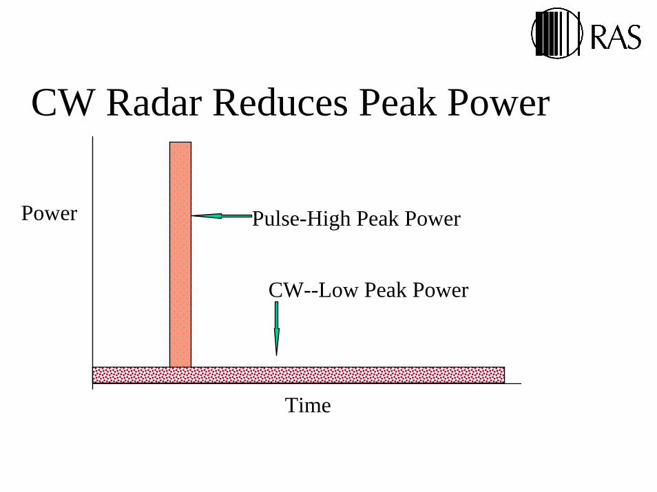
CW Radar Reduces Peak Power

Pulse-High Peak Power

CW--Low Peak Power

Time

Power

History of LPI Radar• Hughes/MICOM 1980s CW/Phase coded

with separate antennas for Tx and Rx. Dev. model only (17Km for 3 sq m target) Later versions were built by other companies.

• Phillips Laboratory-UK devised FM/CW scheme for cancellation of leakage to allow simultaneous Tx/Rx (late 80s)

• Phillips broken up in early 90s.CelsiusTech in Sweden and Signaal in Holland market FM/CW systems

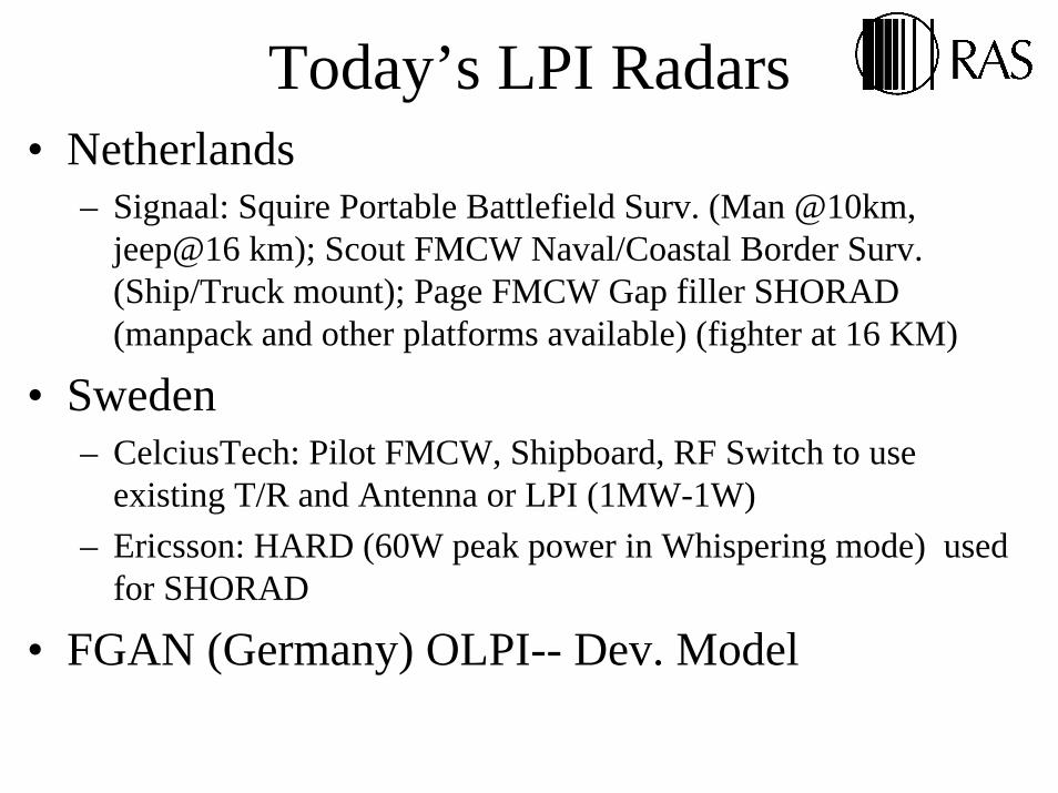
Today’s LPI Radars• Netherlands

– Signaal: Squire Portable Battlefield Surv. (Man @10km, jeep@16 km); Scout FMCW Naval/Coastal Border Surv. (Ship/Truck mount); Page FMCW Gap filler SHORAD (manpack and other platforms available) (fighter at 16 KM)

• Sweden– CelciusTech: Pilot FMCW, Shipboard, RF Switch to use

existing T/R and Antenna or LPI (1MW-1W)– Ericsson: HARD (60W peak power in Whispering mode) used

for SHORAD

• FGAN (Germany) OLPI-- Dev. Model

Random Signal Radar

• Chinese authors publish IEEE-AES paper, July 1999. Reviews history since 1960

• Reviews types of random signal radar • Author Guosui holds a Chinese patent on a

Random FMCW fuse issued in 1987.• Projects future growth due to availability of

DSP and the need for counter-ESM

LPI Radar Sensor

• April 2000 AES Systems Magazine• Authors from Spain• Propose Frequency Hop waveforms as

better for LPI than LFM or PSK when the intercept receiver uses cyclo-stationary spectrum Analysis

Deployed LPI Radars(Last updated in1998)

• Scout: over 130 deployed (per MSSC)• Squire: Development being completed.

Project over 1000 units in 5 years (MSSC)• Page: Production expected in 2002 (MSSC)• Pilot: less than 50 deployed (CelsiusTech)• Hard: (Ericsson)• MICOM: Laboratory only• FGAN: OLPI, Laboratory only

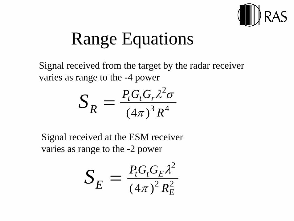
Range Equations

43

2

)4( RGGP

RrttS

πσλ=

Signal received from the target by the radar receiver varies as range to the -4 power

Signal received at the ESM receivervaries as range to the -2 power

22

2

)4( E

Ett

RGGP

ESπ

λ=

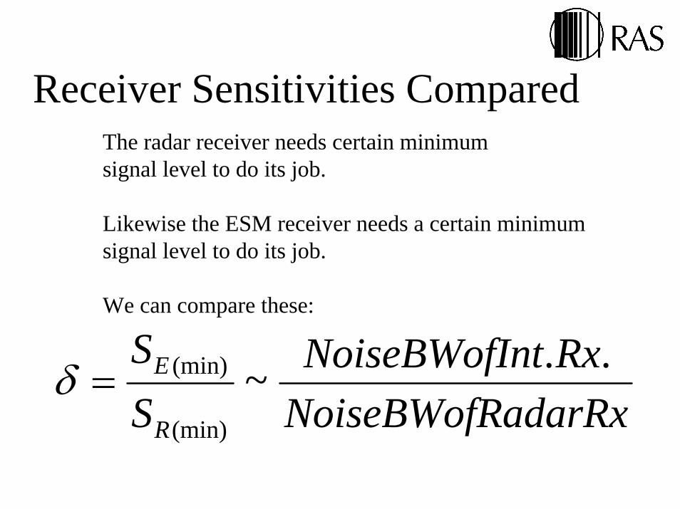
Receiver Sensitivities ComparedThe radar receiver needs certain minimumsignal level to do its job.

Likewise the ESM receiver needs a certain minimumsignal level to do its job.

We can compare these:

adarRxNoiseBWofRRxntNoiseBWofI

SS

R

E ..~(min)

(min)=δ

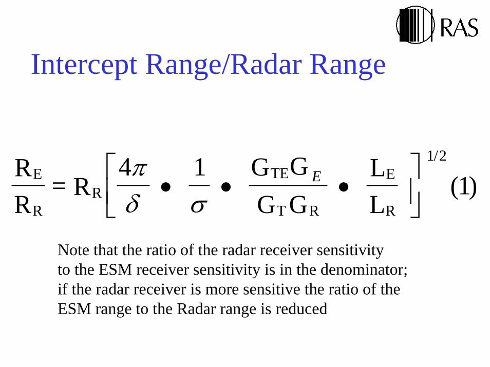
Intercept Range/Radar Range

E

RR

1/2TE

T R

E

R

RR

= R4

1

G GG G

LL

( )πδ σ

• • •⎡⎣⎢

⎤⎦⎥

E 1

Note that the ratio of the radar receiver sensitivity to the ESM receiver sensitivity is in the denominator; if the radar receiver is more sensitive the ratio of theESM range to the Radar range is reduced

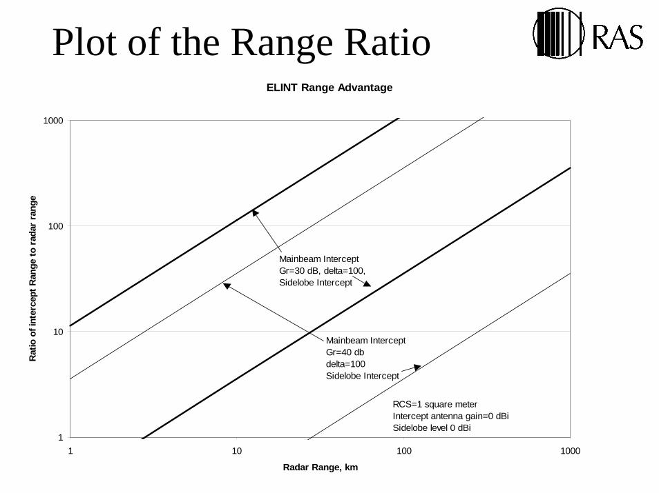
Plot of the Range RatioELINT Range Advantage

1

10

100

1000

1 10 100 1000

Radar Range, km

Rat

io o

f int

erce

pt R

ange

to r

adar

ran

ge

Mainbeam InterceptGr=30 dB, delta=100, Sidelobe Intercept

RCS=1 square meterIntercept antenna gain=0 dBiSidelobe level 0 dBi

Mainbeam InterceptGr=40 dbdelta=100Sidelobe Intercept

Example for Existing Designs

• RCS =1 sq meter• Rx Ant Gain =1, Sidelobe Tx Ant. Gain=1• ESM Rx 20 dB less sensitive than Radar Rx• Then the Sidelobes of the Radar can be

detected at a range of over 30 times the range at which the radar can detect a target

• Main beam detection over1000 times Radar Range

Future ESM Receivers

• 10-30 dB Sensitivity enhancement needed to cope with modern FMCW radar threats

• One way is to use narrow beam, high gain antennas– then a number of receive channels is needed to

cover a given angular sector. Number of receivers and antennas is equal to the antenna gain, i.e.10 to 1000

• Another way is through signal processing

Klipper Equations A way to relate Pre-D SNR and Video SNR

SNR outSNR in

2

2B vB r

.B vB r

2

4B vB r

. SNR in.

SNR in2 SNR out.

B rB v

1 1

2B rB v

. 1

4 SNR out.

12

.

Klipper Equation Example

SNR in 1.8=

B v 6.25 106.=

B r 1 109.=

dB

Hz

Hz

SNR out 11.78= dB

Klipper Equation Comments

• Output SNR is the ratio of the signal envelope power to the noise power at the output of the detector

• Output SNR is not directly useable to obtain Pd and Pfa values from the usual curves

• The Tsui/Albersheim approximations provide the input SNR required to obtain specified Pd and Pfa values.

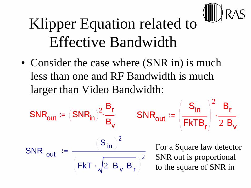
Klipper Equation related to Effective Bandwidth

• Consider the case where (SNR in) is much less than one and RF Bandwidth is much larger than Video Bandwidth:

SNRout SNRin2 Br

Bv

.SNRout SNRin2 Br

Bv

.SNRout SNRin2 Br

Bv

. SNRout

Sin

FkTBr

2 Br

2 Bv

.SNRout

Sin

FkTBr

2 Br

2 Bv

.SNRout

Sin

FkTBr

2 Br

2 Bv

.

SNR out

S in2

FkT 2 B v B r.

2For a Square law detectorSNR out is proportionalto the square of SNR in

Post-Detection Filtering Improves Output SNR

• Improvement is approximately the square root of the ratio of the predetectionbandwidth to twice the post-detection bandwidth (Linear Detector)

• Improvement is relative to the SNR in the Input Band

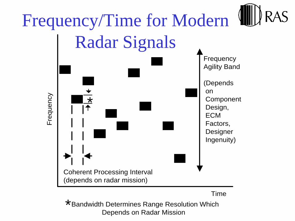
Frequency/Time for Modern Radar Signals

FrequencyAgility Band

(Depends on Component Design, ECM Factors, Designer Ingenuity)

Freq

uenc

y

Coherent Processing Interval(depends on radar mission)

TimeBandwidth Determines Range Resolution Which

Depends on Radar Mission

*

*

Types of “LPI” Radar Modulation

• FMCW (“Chirp”)• Phase Reversals (BPSK)• Other Phase Modulations (QPSK, M-ary

PSK)• In short, any of the pulse compression

modulations used by conventional radar.

“LPI” Radar “Codes”

• True Noise (From a noise source, stored for later correlation in the radar receiver)

• Pseudonoise (nearly unpredictable unless the interceptor has the algorithm and key)

• The code must have good ambiguity properties in range and Doppler. Unpredictability is a plus.

ESM Receiver Strategies• Detection of a random signal radar using

only the energy has the advantage that the detection performance is largely independent of the radar waveform

• Detection based on specific properties of the radar signal can be more efficient

• Radar usage of code/modulation diversity may defeat ESM designed for specific signal properties

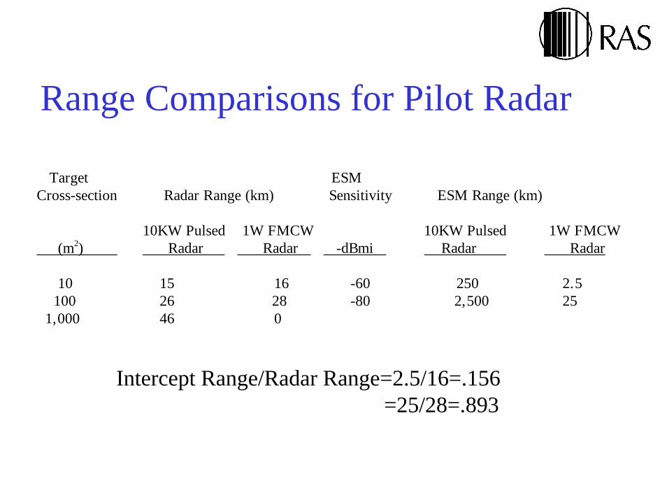
Range Comparisons for Pilot Radar

Target ESM Cross-section Radar Range (km) Sensitivity ESM Range (km)

10KW Pulsed 1W FMCW 10KW Pulsed 1W FMCW (m2) Radar Radar -dBmi Radar Radar

10 15 16 -60 250 2.5 100 26 28 -80 2,500 25 1,000 46 0

Intercept Range/Radar Range=2.5/16=.156=25/28=.893

Signal Processing Techniques

• Non-coherent methods (radiometer) use average power over times comparable to radar’s integration time, e.g., milliseconds (10-15 dB improvement)

• Coherent methods which use “nearly matched” filters, e.g., Wigner Hough Transform for linear FM signals (15-25 dB improvement)

• Cross Correlation method

Non-coherent Approach

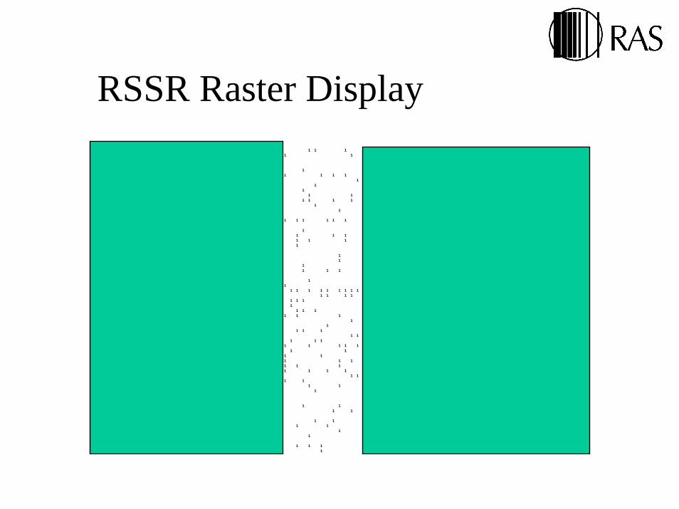
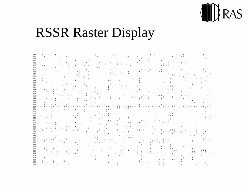
• Rapid Sweep Superhet Receiver (RSSR) proved usefulness of noncoherent or post-detection integration against LPI signals

• Technique should be routinely applied to processing wideband receiver outputs for discovering LPI signals

• Sensitivity improves with square root of n, number of sweeps per pulse

• Hough transform can be applied when chirp exceeds processor IF bandwidth

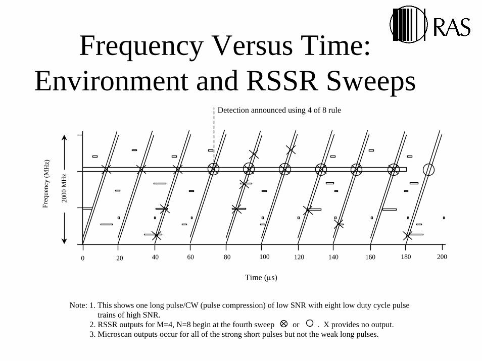
Frequency Versus Time: Environment and RSSR Sweeps

0 20 40 60 80 100 120 140 160 180 200

Detection announced using 4 of 8 rule

2000

MH

z

Freq

uenc

y (M

Hz)

Time (µs)

Note: 1. This shows one long pulse/CW (pulse compression) of low SNR with eight low duty cycle pulsetrains of high SNR.

2. RSSR outputs for M=4, N=8 begin at the fourth sweep or . X provides no output.3. Microscan outputs occur for all of the strong short pulses but not the weak long pulses.

Envelope Techniques

• RSSR uses many samples of the envelope prior to making a detection decision

• Various M/M, M/N and other statistical techniques for sensitivity enhancement can be used

• The past analog implementations could be done digitally in software and applied to a wideband digital data stream

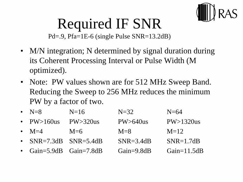
Required IF SNRPd=.9, Pfa=1E-6 (single Pulse SNR=13.2dB)

• M/N integration; N determined by signal duration during its Coherent Processing Interval or Pulse Width (M optimized).

• Note: PW values shown are for 512 MHz Sweep Band. Reducing the Sweep to 256 MHz reduces the minimum PW by a factor of two.

• N=8 N=16 N=32 N=64• PW>160us PW>320us PW>640us PW>1320us• M=4 M=6 M=8 M=12• SNR=7.3dB SNR=5.4dB SNR=3.4dB SNR=1.7dB• Gain=5.9dB Gain=7.8dB Gain=9.8dB Gain=11.5dB

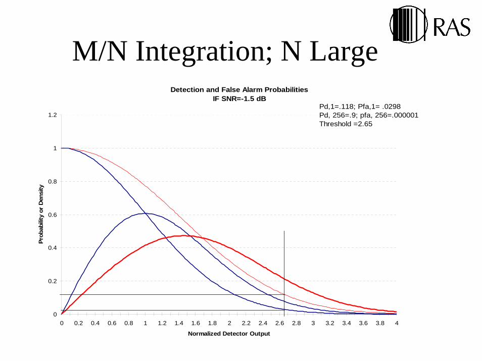
M/N Integration; N LargeDetection and False Alarm Probabilities

IF SNR=-1.5 dB

0

0.2

0.4

0.6

0.8

1

1.2

0 0.2 0.4 0.6 0.8 1 1.2 1.4 1.6 1.8 2 2.2 2.4 2.6 2.8 3 3.2 3.4 3.6 3.8 4

Normalized Detector Output

Prob

abili

ty o

r D

ensi

ty

Pd,1=.118; Pfa,1= .0298Pd, 256=.9; pfa, 256=.000001Threshold =2.65

RSSR Raster Display3 9 0 1 1 1 1 1 1 1 1 1 1 1 1 1 3 9 4 1 1 1 1 1 1 1 1 1 1 1 1 3 9 8 1 1 1 1 1 1 1 1 4 0 2 1 1 1 1 1 1 1 1 1 14 0 6 1 1 1 1 1 1 1 1 1 1 4 1 0 1 1 1 1 1 1 1 1 1 4 1 4 1 1 1 1 1 1 1 1 1 1 1 1 1 1 1 4 1 8 1 1 1 1 1 1 1 1 1 4 2 2 1 1 1 1 1 1 1 1 1 1 1 1 1 1 1 1 4 2 6 1 1 1 1 1 1 1 1 1 1 1 1 4 3 0 1 1 1 1 1 1 1 1 14 3 4 1 1 1 1 1 1 1 1 1 1 1 4 3 8 1 1 1 1 1 1 1 1 4 4 2 1 1 1 1 1 1 1 1 1 1 1 4 4 6 1 1 1 1 1 1 1 1 1 1 1 1 1 1 1 1 4 5 0 1 1 1 1 1 1 1 1 1 4 5 4 1 1 1 1 1 1 4 5 8 1 1 1 1 1 1 1 1 1 1 4 6 2 1 1 1 1 1 1 1 1 1 1 4 6 6 1 1 1 1 1 1 1 1 1 1 1 1 1 14 7 0 1 1 1 1 1 1 1 1 1 1 1 1 1 4 7 4 1 1 1 1 1 1 1 1 1 1 1 1 1 1 14 7 8 1 1 1 1 1 1 1 1 1 1 1 1 1 1 1 1 1 4 8 2 1 1 1 1 1 1 1 1 1 1 1 1 4 8 6 1 1 1 1 1 1 1 1 1 1 1 1 1 1 1 1 1 14 9 0 1 1 1 1 1 1 1 1 4 9 4 1 1 1 1 1 1 1 1 1 1 1 1 4 9 8 1 1 1 1 1 1 1 1 1 1 1 1 15 0 2 1 1 1 1 1 1 1 1 1 1 1 1 1 1 1 1 1 1 1 1 1 1 1 1 1 1 1 1 1 1 1 1 1 1 1 1 1 1 1 1 1 1 1 1 1 1 1 1 1 1 1 1 1 1 15 0 6 1 1 1 1 1 1 1 1 5 1 0 1 1 1 1 1 1 1 1 1 1 1 5 1 4 1 1 1 1 1 1 1 1 1 5 1 8 1 1 1 1 1 1 1 1 1 1 1 1 1 5 2 2 1 1 1 1 1 1 1 1 1 1 1 1 1 1 15 2 6 1 1 1 1 1 1 1 15 3 0 1 1 1 1 1 1 5 3 4 1 1 1 1 1 1 1 1 1 1 5 3 8 1 1 1 1 1 1 1 1 1 1 1 1 1 5 4 2 1 1 1 1 1 1 1 1 1 1 1 5 4 6 1 1 1 1 1 1 1 1 1 1 1 1 1 5 5 0 1 1 1 1 1 1 1 1 1 1 1 5 5 4 1 1 1 1 1 1 1 1 1 1 1 1 1 1 1 1 1 1 1 5 5 8 1 1 1 1 1 1 1 1 1 1 1 1 1 1 1 5 6 2 1 1 1 1 1 1 1 1 1 1 1 1 5 6 6 1 1 1 1 1 1 1 1 1 1 1 5 7 0 1 1 1 1 1 1 1 1 1 1 5 7 4 1 1 1 1 1 1 1 1 1 1 1 1 1 15 7 8 1 1 1 1 1 1 1 1 1 1 1 1 1 5 8 2 1 1 1 1 1 1 1 1 1 1 1 5 8 6 1 1 1 1 1 5 9 0 1 1 1 1 1 1 1 1 5 9 4 1 1 1 1 1 1 1 1 1 1 1 5 9 8 1 1 1 1 1 1 1 1 1 1 1 6 0 2 1 1 1 1 1 1 1 1 1 1 1 1 1 1 16 0 6 1 1 1 1 1 1 1 1 1 1 1 6 1 0 1 1 1 1 1 1 1 1 1 1 1 6 1 4 1 1 1 1 1 1 1 1 1 1 6 1 8 1 1 1 1 1 1 1 1 1 1 6 2 2 1 1 1 1 1 1 1 1 6 2 6 1 1 1 1 1 1 1 1 1 1 1 1 1 1 6 3 0 1 1 1 1 1 1 1 1 1 1 1 1 1 1

“Coherent” Approaches• “Coherent” means processing prior to the

envelope detector• Cross-Correlation using two or more channels--

performance independent of waveform• Frequency-Time Processing detects CHIRP or

CW signals in Noise ( e.g.,Wigner-Hough Transform)– Time coincident pulses detected separately

Cross-Correlation Method

• Requires two channels with two antennas• Sensitivity enhancement can be sufficient to

deal with modern LPI FMCW radars on the battlefield (“almost coherent”)

• Processes all modulation types equally well (Phase codes as well as FM)

• Provides AOA, Frequency and Bandwidth information

Cross-Correlation Block Diagram

X

~ X

CrossCorrelator

ct d

Antennas

Low-Noise RFAmplifiers Mixers

Weak Spread-Spectrum Signal

d

Stable Low-Noise

Oscillator

θ

XLNA

LNA

FourierTransform

Cross-Correlation (con’t)

• Does not provide knowledge of the modulation type

• Modulation may be determined via high gain antenna directed toward the AOA of the LPI signal (dedicated ESM Rx)

• Significant signal processing load• Wideband Cross-Correlation (large BT)

beyond the current State-of-the-art(?)

Choosing CorrrelationParameters

• Correlation Time (T) is on the order of the radar’s time on target or Integration time (Typically 1-10 ms) Long enough to provide integration gain but not so long that the signal changes “very much”

• Receiver Bandwidth (B): wide to minimize search time; narrow to minimize noise and A/D speed. (Several times wider than the likely modulation bandwidths.)

Time-Frequency Transforms (Relationships and Descriptions)

• Wigner-Ville Distribution (WVD)– Good Time-Frequency resolution– Cross-term interference (for multiple signals), which is:

• Strongly oscillatory• Twice the magnitude of autoterms • Midway between autoterms• Lower in energy for autoterms which are further apart

• Ambiguity Function (AF)– AF is the 2D Fourier Transform of the WVD– A correlative Time-Frequency distribution

• Choi-Williams Distribution (CWD)– Used to suppress WVD cross-term interference (for multiple signals),

though preserves horizontal/vertical cross-terms in T-F plane– Basically a low-pass filter

• Time-Frequency Distribution Series (Gabor Spectrogram) (TFDS)– Used to suppress WVD cross-term interference (for multiple signals) by:

• Decomposing WVD into Gabor expansion• Selecting only lower order harmonics (which filters cross-term interference)

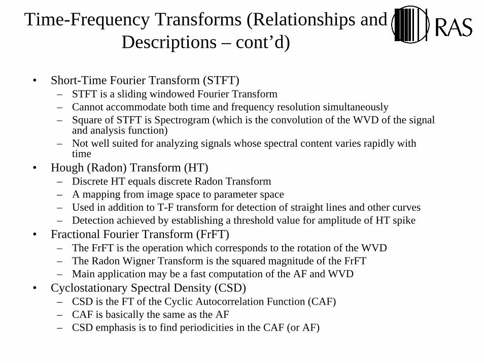
Time-Frequency Transforms (Relationships and Descriptions – cont’d)

• Short-Time Fourier Transform (STFT) – STFT is a sliding windowed Fourier Transform– Cannot accommodate both time and frequency resolution simultaneously– Square of STFT is Spectrogram (which is the convolution of the WVD of the signal

and analysis function)– Not well suited for analyzing signals whose spectral content varies rapidly with

time• Hough (Radon) Transform (HT)

– Discrete HT equals discrete Radon Transform– A mapping from image space to parameter space– Used in addition to T-F transform for detection of straight lines and other curves– Detection achieved by establishing a threshold value for amplitude of HT spike

• Fractional Fourier Transform (FrFT)– The FrFT is the operation which corresponds to the rotation of the WVD– The Radon Wigner Transform is the squared magnitude of the FrFT– Main application may be a fast computation of the AF and WVD

• Cyclostationary Spectral Density (CSD) – CSD is the FT of the Cyclic Autocorrelation Function (CAF)– CAF is basically the same as the AF– CSD emphasis is to find periodicities in the CAF (or AF)

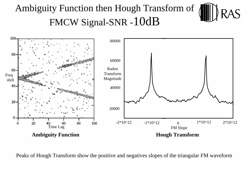
Ambiguity Function then Hough Transform of FMCW Signal-SNR -10dB

80000

60000

RadonTransformMagnitude

Freqshift

Time Lag

Ambiguity Function

40000

20000

2*10^120-1*10^12-2*10^12 1*10^12FM Slope

Hough Transform

Peaks of Hough Transform show the positive and negatives slopes of the triangular FM waveform

WVD and CWD comparison forLFM signal (SNR -15dB)

20 40 60 80 100 120

20

40

60

80

100

120

WVD of LFM signal in noise

CWD of LFM signal in noise

HT of WVD of LFM signal in noise

HT of CWD of LFM signal in noise

WVD has better T-F resolution and a ‘tighter’ HT spike. 1 WVD/CWD line maps to 1 HT spike. Detection achieved via establishing a threshold value for the amplitude of the HT spike

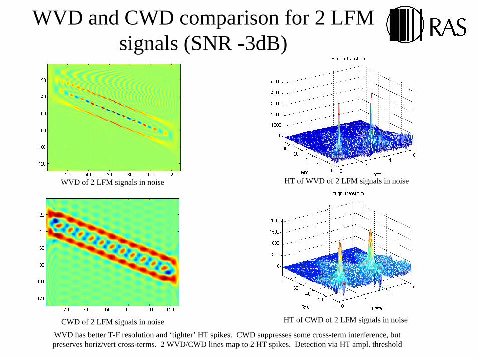
WVD and CWD comparison for 2 LFM signals (SNR -3dB)

WVD of 2 LFM signals in noise

CWD of 2 LFM signals in noise

HT of WVD of 2 LFM signals in noise

HT of CWD of 2 LFM signals in noise

WVD has better T-F resolution and ‘tighter’ HT spikes. CWD suppresses some cross-term interference, but preserves horiz/vert cross-terms. 2 WVD/CWD lines map to 2 HT spikes. Detection via HT ampl. threshold

STFT of LFM signal and of 2 LFM signals(SNR -3dB)

STFT of LFM signal in noise

STFT of 2 LFM signals in noise

HT of STFT of LFM signal in noise

HT of STFT of 2 LFM signals in noise1 STFT line maps to 1 HT spike; 2 STFT lines map to 2 HT spikes. STFT T-F resolution inferior to that of WVD (STFT-window funct. imposes resolution limit). STFT superior to WVD for cross-term interf. Detection via HT ampl. threshold

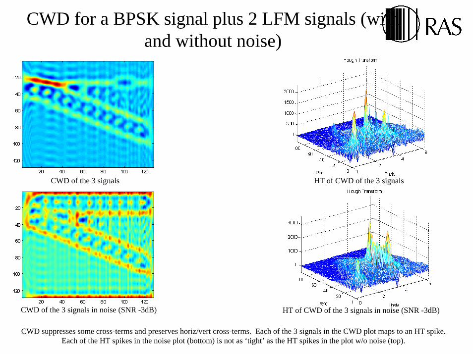
CWD for a BPSK signal plus 2 LFM signals (with and without noise)

CWD of the 3 signals HT of CWD of the 3 signals

CWD of the 3 signals in noise (SNR -3dB) HT of CWD of the 3 signals in noise (SNR -3dB)

CWD suppresses some cross-terms and preserves horiz/vert cross-terms. Each of the 3 signals in the CWD plot maps to an HT spike. Each of the HT spikes in the noise plot (bottom) is not as ‘tight’ as the HT spikes in the plot w/o noise (top).

Heuristic AnalysisFrequency Hopper

STFT

WVD CWD

TFDS (3rd order)

WVD has best T-F resolution, but nasty cross-term interference. CWD suppresses some cross-terms, but preserves horiz/vert cross-terms. STFT has worst T-F resol., but no cross-terms. TFDS (3rd order) has best combo of T-F res. and limited cross-terms for this waveform.

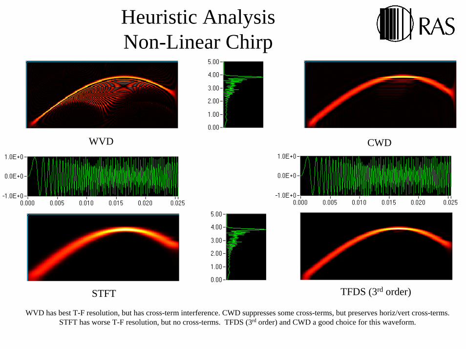
Heuristic AnalysisNon-Linear Chirp

WVD CWD

STFT TFDS (3rd order)

WVD has best T-F resolution, but has cross-term interference. CWD suppresses some cross-terms, but preserves horiz/vert cross-terms. STFT has worse T-F resolution, but no cross-terms. TFDS (3rd order) and CWD a good choice for this waveform.

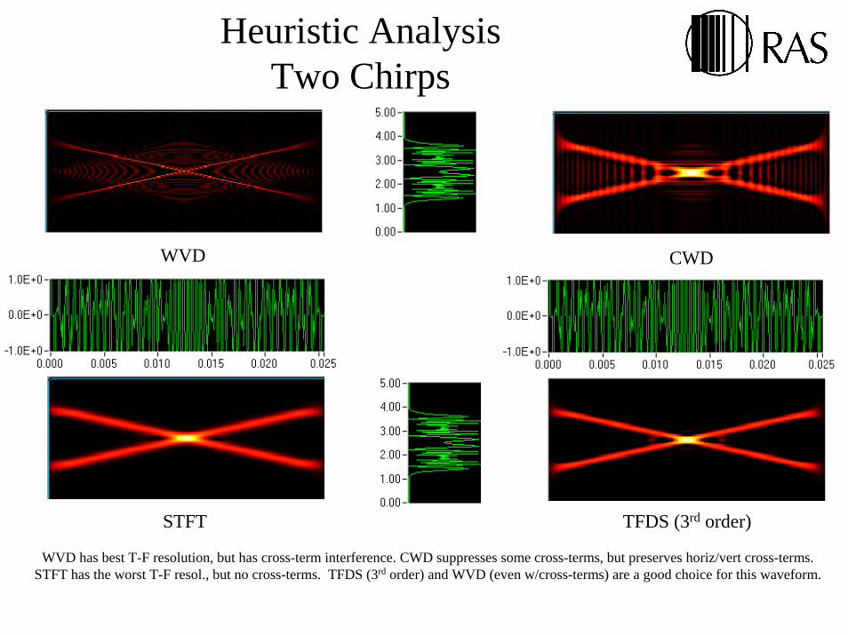
Heuristic AnalysisTwo Chirps

WVD CWD

STFT TFDS (3rd order)

WVD has best T-F resolution, but has cross-term interference. CWD suppresses some cross-terms, but preserves horiz/vert cross-terms. STFT has the worst T-F resol., but no cross-terms. TFDS (3rd order) and WVD (even w/cross-terms) are a good choice for this waveform.

Predetection ESM Sensitivity Enhancement

• Wigner-Hough Transform– Approaches Coherent Integration– “Matched” to Chirp and Constant MOP– Separation of Simultaneous Pulses

• Provides Parametric information about Frequency and Chirp Rate

Wigner-Hough Transform

Wigner Ville Transform

W t f x t x t e d

Wigner Hough Transform

WH f g W t g t dtd

W t f g t dt

x xj f

x x x x

x x

−

= + ⋅ − ⋅

−

= − ⋅

= + ⋅

−

=−∞

∞

∫

∫∫∫

,*

, ,

,

( , ) ( ) ( )

( , ) ( , ) ( )

( , )

τ τ τ

ν δ ν ν

π τ

τ2 2 2

W-H Transform Example

• 20 MHz Chirp• 1 usec Pulse Duration• 200 MHz Sample Rate

0 0.2 0.4 0.6 0.-1

-0.5

0

0.5

1IF of Channe l

Time (usec)

0 20 40 60-60

-40

-20

0

20

Frequency (MHz)

Pow

er (d

B)

P ower S pectra l Density of

W-H Transform (12 dB SNR)

2030

4050

60

0

0.5

1

x 10-3

0

1000

2000

3000

4000

5000

6000

Frequency (MHz)Normalized Chirp Ra te 20 25 30 35 40 450

0.1

0.2

0.3

0.4

0.5

0.6

0.7

0.8

0.9

1x 10-3

Frequency (MHz)

Nor

mal

ized

Chi

rp R

ate

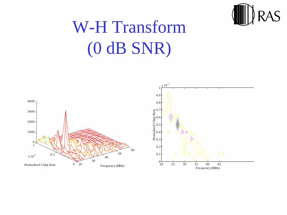
W-H Transform (0 dB SNR)

2030

4050

60

0

0.5

1

x 10-3

0

1000

2000

3000

4000


0.1

0.2

0.3

0.4

0.5

0.6

0.7

0.8

0.9

1x 10-3

Frequency (MHz)

Nor

mal

ized

Chi

rp R

ate

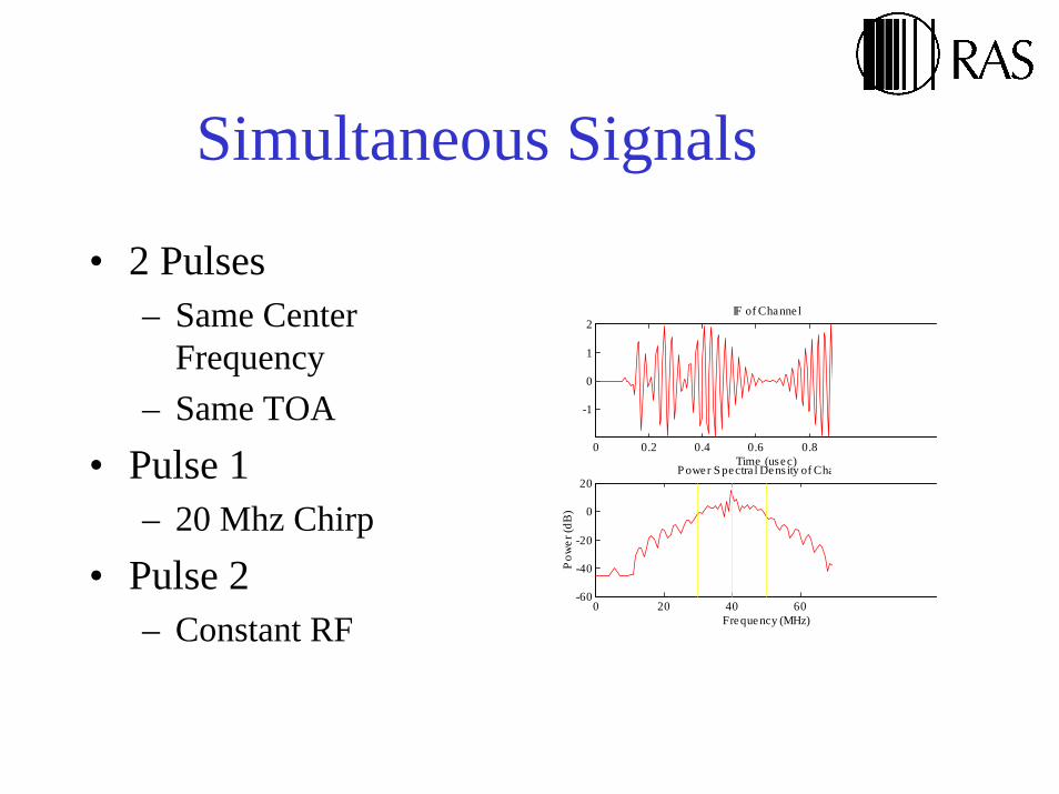
Simultaneous Signals

• 2 Pulses – Same Center

Frequency– Same TOA

• Pulse 1– 20 Mhz Chirp

• Pulse 2– Constant RF

0 0.2 0.4 0.6 0.8

-1

0

1

2IF of Channe l

Time (usec)

0 20 40 60-60

-40

-20

0

20

Frequency (MHz)

Pow

er (d

B)

P ower S pectra l Dens ity of Cha

W-H Transform-simultaneous signals

2030

4050

60

0

0.5

1

x 10-3

0

1000

2000

3000

4000

5000


0.1

0.2

0.3

0.4

0.5

0.6

0.7

0.8

0.9

1x 10-3

Frequency (MHz)

Nor

mal

ized

Chi

rp R

ate

Summary• Each T-F transform has its own strengths and weaknesses, and is very much

application dependent, thusly a need to produce multiple algorithms for multiple applications

• T-F transforms are especially useful for recognizing wideband signals, non-stationary signals, and signals buried in noise

• Many of the T-F transforms and inter-related with one another• WVD yields the best overall T-F resolution, but for multiple signals, is

plagued with cross-term interference• CWD, TFDS, and other T-F transforms can suppress cross-term interference,

but at the cost of T-F resolution • TFDS allows specific selection of order which makes for a good compromise

between T-F resolution and cross-term interference• STFT is not plagued with cross-term interference, but cannot accommodate

both time and frequency resolution simultaneously (subject to the selection of the window function). To ‘catch’ abrupt frequency jumps, the STFT must use a very short window, and is not recommended for very rapidly changing frequencies

• Hough Transform can be applied to a T-F transform and then used for the detection of straight lines and other curves. An HT amplitude threshold can be set for detection

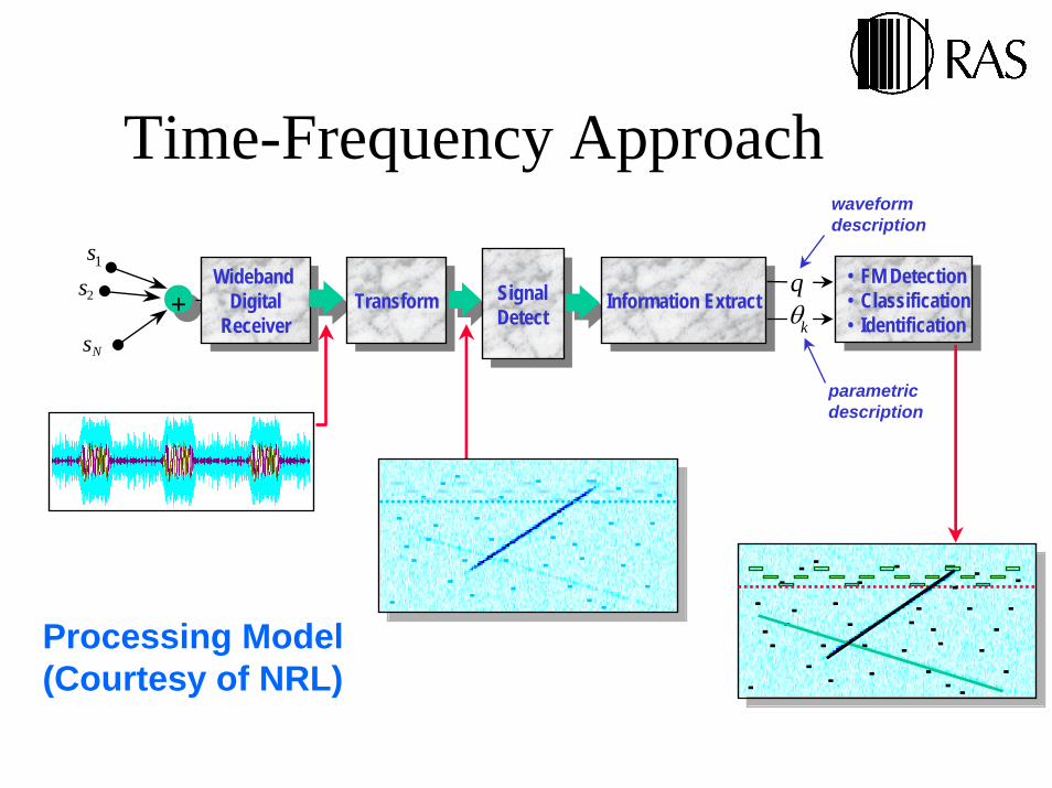
Time-Frequency Approach

Processing Model(Courtesy of NRL)

• FM Detection• Classification• Identification

• FM Detection• Classification• Identification

+

s1

s2

sN

WidebandDigital

Receiver

WidebandDigital

ReceiverTransformTransform Signal

DetectSignalDetect Information ExtractInformation Extract

qkθ

waveformdescription

parametricdescription

Modern Receivers for Modern Threats

• Integration over times on the order of 1-10 ms over bandwidths on the order of 100 MHz. are required to cope with short range FMCW or Phase coded radars expected on the modern battlefield. (BT~10, 000-100,000)

• Fast A/D conversion and DSP are the keys to implementation of these ESM strategies.

intercepting modern signals - ieee well as low power long duration signals are present • today’s...

Documents