IAEA-TECDOC-882

Intercomparison ofliquid metal fast reactorseismic analysis codes

Volume 3:Comparison of observed effectswith computer simulated effects

on reactor coresfrom seismic disturbances

Proceedings of a final Research Co-ordination Meetingheld in Bologna, Italy, 30 May-2 June 1995

INTERNATIONAL ATOMIC ENERGY AGENCY 11 /A\

May 1996

The IAEA does not normally maintain stocks of reports in this series.However, microfiche copies of these reports can be obtained from

INIS ClearinghouseInternational Atomic Energy AgencyWagramerstrasse 5P.O. Box 100A-1400 Vienna, Austria

Orders should be accompanied by prepayment of Austrian Schillings 100,in the form of a cheque or in the form of IAEA microfiche service couponswhich may be ordered separately from the INIS Clearinghouse.

The originating Section of this publication in the IAEA was:Nuclear Power Technology Development Section

International Atomic Energy AgencyWagramerstrasse 5

P.O. Box 100A-1400 Vienna, Austria

INTERCOMPARISON OF LIQUID METAL FAST REACTOR SEISMIC ANALYSIS CODESVOLUME 3:

COMPARISON OF OBSERVED EFFECTS WITH COMPUTER SIMULATED EFFECTSON REACTOR CORES FROM SEISMIC DISTURBANCES

IAEA, VIENNA, 1996IAEA-TECDOC-882

ISSN 1011-4289

© IAEA, 1996

Printed by the IAEA in AustriaMay 1996

FOREWORD

One of the primary requirements for nuclear power plants and facilities is to ensuresafety and the absence of damage under strong external dynamic loadings such asearthquakes. The designs of liquid metal fast reactors (LMFRs) include systems whichoperate at low pressure and components which are thin-walled and flexible. These featuresmay be severely affected by earthquakes. Therefore, the International Atomic Energy Agencysupports the activities of Member States to apply seismic isolation technology to LMFRs inadvanced reactor technology development.

The IAEA organizes meetings and co-ordinated research programmes in which MemberStates exchange experimental and analytical data. The IAEA has sponsored two meetings onthe seismic behaviour of LMFRs: Reactor-block anti-seismic design and verification(Bologna, Italy, October 1987) and seismic isolation technology (San Jose, California, March1992). The participants of the first meeting recommended performing benchmark analysesto compare and validate the computer codes developed in different countries. This proposalwas consistent with the conclusion that detailed core seismic analysis was important to ensurefast reactor safety during an earthquake. The IAEA Working Group on LMFR endorsed thisproposal at its meeting in April 1990 and after that year the IAEA approved the Co-ordinatedResearch Programme (CRP) on Intercomparison of LMFR Seismic Analysis Codes.

The codes used for the structural design of the core and reactor internals were validatedin two stages. The first stage was the comparison of the analytical results with the ItalianPEC reactor core experiments. In stage two the Japanese and French reactor coreexperiments were compared.

The results have been published in the following two volumes:

Volume 1 : Validation of Seismic Analysis Codes using Reactor Core Experiments (IAEA-TECDOC-798)

Volume 2: Verification and Improvement of Reactor Core Seismic Analysis Codes usingCore Mock-up Experiments (IAEA-TECDOC-829).

This publication (Volume 3) contains the final papers summarizing the validation of thecodes on the basis of comparison of observed effects with computer simulated effects onreactor cores from seismic disturbances.

EDITORIAL NOTE

In preparing this publication for press, staff of the IAEA have made up the pages from theoriginal manuscripts as submitted by the authors. The views expressed do not necessarily reflect thoseof the governments of the nominating Member States or of the nominating organizations.

Throughout the text names of Member States are retained as they were when the text wascompiled.

The use of particular designations of countries or territories does not imply any judgement bythe publisher, the IAEA, as to the legal status of such countries or territories, of their authorities andinstitutions or of the delimitation of their boundaries.

The mention of names of specific companies or products (whether or not indicated as registered)does not imply any intention to infringe proprietary rights, nor should it be construed as anendorsement or recommendation on the part of the IAEA.

The authors are responsible for having obtained the necessary permission for the IAEA toreproduce, translate or use material from sources already protected by copyrights.

CONTENTS

Summary of the final meeting and co-ordinated research programme . . . . . . . . . . 7

Seismic response analysis of FBR core by FIN AS code . . . . . . . . . . . . . . . . . . 13M. Morishita

Seismic response analysis of Rapsodie core mock-up in water experiment . . . . . . . 38M. Morishita

Verification and validation analysis on LMFBR core mock-up seismicexperiments by FINDS code . . . . . . . . . . . . . . . . . . . . . . . . . . . . . . . 61K. Itoh, T. Satoh, I. Aizawa

Evaluation of LMFBR core seismic analysis by the SALCON code . . . . . . . . . . . 113T. Kobayashi

Analysis of the core seismic experiments using the SAFA programfor intercomparison of LMFBR seismic analysis codes . . . . . . . . . . . . . . . . 151T. Horiuchi

Seismic analysis for Monju core seismic experiments using the SAFA program . . . . 179T. Horiuchi

Final report on results of calculation by CORE-SEIS . . . . . . . . . . . . . . . . . . . . 201A. Ravi, P. Chellapandi, T. Selvaraj, S.C. Chetal, S.B. Bhoje

Analysis of the core seismic experiments using the COSMOS/M code . . . . . . . . . . 227K.K. Vaze, B. Murli

Seismic analysis of Monju and Rapsodie LMFBR core mock-ups . . . . . . . . . . . . . 297B. Fontaine, F. Gantenbein

List of Participants . . . . . . . . . . . . . . . . . . . . . . . . . . . . . . . . . . . . . . . . . . . . . . 3 1 3

SUMMARY OF THE FINAL MEETING AND OF THECO-ORDINATED RESEARCH PROGRAMME

The final Research Co-ordination Meeting held in Bologna, Italy, from 30 May to2 June 1995, was attended by participants from France, India, Italy, Japan and the RussianFederation. The meeting reviewed the benchmark results obtained by various organizationsfor the analysis of Italian, French and Japanese tests on PEC, RAPSODIE and MONJUmock-ups. The key objective was an overall review of the validation results of seismicanalysis methods and codes for the LMFR core, using the reactor core mock-up experiments.

Analyses performed by the participating organizations

Japan: As the final report of the CRP, M. Morishita presented an overview of PNC'sanalysis work with the FINAS code on the PEC, MONJU, and RAPSODIE core mock-upexperiments. Although these experiments varied in size, number of subassemblies, coreconfigurations (free-standing or restrained), and excitation conditions, the results by FINAScode in general were in accordance with reasonably accurate experimental data. From theseresults, he concluded that the present analysis method with the FINAS code was judged tobe capable of practical use. In addition, he also pointed out that there was room for furtherimprovement in the shock calculations (especially for MONJU, in which the shock stiffnessis very high) and the fluid-structure interaction modelling (especially for RAPSODIE, inwhich the annulus between the core and the vessel is very narrow). He made someintercomparison of the analysis results obtained by the participants' codes in some cases. Forthe PEC and MONJU experiments, they gave fairly close results to each other and to theexperiments. For example, the variation in the displacement results was within 20% for thePEC experiments. However, the variation among the codes was relatively large for theRAPSODIE experiment, which he attributed to the large number of subassemblies in themock-up. Finally, he identified some issues for further study from the viewpoint of morereliable seismic qualification of FBR core, which included fluid-structure interaction,response to 2-D horizontal excitations, response to base isolation conditions, response tovertical excitations, and the effect of pin bundles.

M. Morishita also presented, on behalf of T. Kobayashi, Toshiba Corp., the final reporton the results by the SALCON code. For the PEC and MONJU experiments, concurrencewas seen between the analysis and the experiments in terms of displacement responses. Asfor the RAPSODIE experiment in air, the calculated displacement also agreed with theexperiment. Several analyses were made for the test in water, with the parameter changingregarding the fluid-structure interaction effect. Although good results were obtained, the needfor additional information to confirm the validity of the selected calculation condition waspointed out. T. Kobayashi also studied the effects of the direction of the input seismic load(flat-to-flat or corner-to-corner), by comparing the results of analyses on PEC experiments.The study concluded that the effect of input direction is negligible and use of single rowmodels with flat-to-flat input for seismic design purposes is justified.

T. Horiuchi made presentations on his and of K. Itoh's, Mitsubishi Heavy Industry,Japan, behalf. In the first presentation, T. Horiuchi showed his calculation results mainly onMonju experiments. He discovered that it was difficult to obtain good results in the collisiontest with the provided stiffness, therefore, he used a modified stiffness in the seismiccalculations. In the comparisons of displacements and impact forces, he obtained close valuesto those measured in the calculations. However, the calculated strains were smaller than themeasured ones. He decided that this was caused by impulsive strain made by impact, which

cannot be considered in the calculation model. His conclusion, obtained from thesecalculations, was that the code used in the calculations, SAP A, was verified to be of practicaluse. His recommendation for future research was to obtain precise vibration characteristics,based on experiments and clarity of design criteria, for determination targets of programimprovements. Also, he noted that research on the method of considering fluid force isimportant.

In his second presentation, T. Horiuchi displayed reviews of calculations made byK. Itoh, using Mitsubishi's original code, FINDS. Although there were some discrepancieshi the calculated results, which may be caused by uncertainty of input parameters, K. Itohconcluded that FINDS can simulate the response of core structures well. In addition, theresults of the Monju experiment using not FINDS, but the ANSYS code, a general-purposeFEM code, were shown. They were satisfactory in both displacements and impact forces.K. Itoh's report contains some recommendations for future research, including theclarification of design criteria, such as control-rod-insertion time and structural integrity ofsubassemblies.

India: K.K. Vaze made a presentation of the final reports on the analyses performedat the Bhabha Atomic Research Centre (BARC), Bombay, and Indira Gandhi Centre forAtomic Research (IGCAR), Kalpakkam.

At BARC, analyses were performed using a general purpose code, COSMOS. Thefollowing observations were made:

(1) The natural frequencies could be predicted well in most cases;

(2) The displacement responses compared well with the experiment, and calculated valuesshowed good agreement with observed values, both in magnitude and frequency content;

(3) The accelerations were overly protected, which could be due to the filtering of data inexperiments resulting from rather large tune intervals between data acquisition.

At IGCAR, the analyses were performed using the in-house CORE-SEIS code. Theobservations were similar to those made by BARC: (1) For the MONJU tests, the high localstiffness posed numerical difficulties necessitating some adjustment, and (2) The RAPSODIEtest was analysed as a row model and good results were obtained for fuel assemblies.However, the results for neutron shield elements showed larger discrepancies.

The overall conclusions are:

(1) It is necessary to perform simple tests on single assembly and on small clusters. Basedon these tests, the parameters of numerical models, such as structural damping, shockstiffness, shock damping, etc., need to be tuned to get the measured frequencies andimpact forces,

(2) Using the numerical models, based on limited test data, the computer codes cancalculate the seismic response of LMFBR cores with good accuracy.

It was recommended that the studies be extended to:

design issues, such as reactivity changes including effect of vertical ground motion,control rod insertability, etc.;

backward integration into computer codes for calculating the response of the reactorblock. It was suggested that calculations could be performed for a reference pool typeLMFBR. Seismic isolation can also be incorporated in these studies.

Russian Federation: As the final report of the CRP, V. Silaev presented an overviewof OKBM's analysis work with the DINARA code on the PEC, MONJU and RAPSODIEcore mock-up experiments. Tests were performed in air and in water. He reviewed state-of-the-art seismic experimental and analytical activities of OKBM, described the core seismicanalysis computer codes and summarized the work done during 1990-1995. V. Silaev alsodescribed the results of validation and verification of the DINARA code, using the reactorcore mock-up experiments. His conclusion, obtained from calculations, is that the DINARAcode used in calculations was verified and can be used for practical purposes.

Italy: A. Martelli presented the analysis of the results of shake table tests in air andwater on the RAPSODIE core mock-up performed by ENEA. The features of the analyseswere explained in detail in Vol. 2 of the proceedings of CRP activities (IAEA-TECDOC-829).

The ENEA study (which was carried out using both the ID code CORALIE and the 2Dcode CLASH), aimed at fully assessing the fluid-structure interaction (ESI) model applicableto the seismic analysis of restrained LMFR cores. The first goal was to check the adequacyof the model that had been previously developed, based on the results of shake table tests ofgroups of 7 and 19 PEC core elements (see IAEA-TECDOC-798). The second goal was toimprove this model so as to account for the effects of the relatively small thickness of theliquid layer which surrounds the core. Both goals were achieved, in spite of someuncertainties related to the core geometry (clearances at neutron element top), shock stiffnessand element restraint conditions (non perfect encastre for the neutron shield elements).

France: B. Fontaine's presentation concerned the Rapsodie core mock-up experiments.Most of the results were presented at the last CRP meeting. The main subject of thepresentation were new water test calculations. After a brief description of the subassemblymodels, the results of in-air tests were presented/discussed. It can be seen that the profile ofdisplacement obtained from calculation was very close to the experimental one, despite somediscrepancies concerning neutronic shield elements. Following the in-air tests, the in-watertest results were presented. An important point was made on the determinations of thedecrease of the seismic input, caused by the coupling of assemblies and vessel: without thisdecrease the calculations greatly over-estimated the displacements of assemblies.

Conclusions and recommendations of the CRP

Nine organizations from five countries participated in the CRP: CEA (France), ENEA(Italy), IGCAR and BARC (India), OKBM (the Russian Federation), HITACHI,MITSUBISHI, PNC, and TOSHIBA (Japan). Three of them provided experimental data forthe benchmark study of the reactor core:

- France (CEA): RAPSODIE mock-up (291 elements' cluster);- Italy (ENEA): PEC mock-ups (to 19 elements);

Japan (PNC): MONJU mock-ups (29 elements hi a line, and 37 elements' cluster).

Data concerned tests in air and water, and included measured results for displacements,accelerations and shock forces. These were analysed using the following computer codes:

- CASTEM-2000 (CEA);- CORALIE and CLASH (ENEA);- FINAS (PNC);- FINDS (MITSUBISHI);- SAP A (HITACHI);- SALCON (TOSHIBA);- CORE-SEIS (IGCAR);- COSMOS (BARC);- DINARA (OKBM).

The codes used for the seismic analysis were verified and unproved through benchmarkanalysis with existing experimental data.

Three Research Co-ordination Meetings (16-17 November 1993, Vienna, Austria, 26-28September 1994, Oarai, Japan, 30 May-2 June 1995, Bologna, Italy) were dedicated todiscussing and reviewing the data and to validating LMFR structural codes.

The general conclusions of the analyses can be summarized as follows:

• When the same input data were used, all codes gave consistent results in spite ofdifferences hi the methodologies (modal superposition or direct integration, etc.)

• In some cases, dynamic line analysis of the core (limited to the elements in the corediameter) may be sufficiently accurate; however, this feature should be carefullychecked in each case.

• Concerning the fluid effects, in order to correctly evaluate both natural frequencies inthe liquid and the effects on seismic load, an accurate definition of the values of bothdiagonal and non-diagonal terms of the added mass matrix is necessary.

• Analysis of some test data indicates that fluid effects on damping are limited.

• The effects of possible clearances at the spike of core elements have to be carefullytaken into account, depending on the excitation level.

• Shock stiffness, damping, and integration time step in the shock model used in the non-linear core analysis should be carefully determined; the values of shock parametersshould take into account the possibility of simultaneous shocks on different hexagonalfaces.

• The presence of some input data uncertainties (e.g. restraint conditions, gaps, shockstiffness, seismic input, natural frequency values, etc.) complicated the analysis, but didnot prevent conclusions from being reached on the main topics.

The study produced the following recommendations:

• Seismic analysis of the core requires good data (geometry, natural frequencies in air andliquid, restraint conditions, stiffness of hexane section at shock locations, etc.).

• Experimental validation and calibration of numerical models should use maximumresponse values, tune-histories, RMS values and results in the frequency domain.

10

• More experimental evidence is needed to support the indication that the damping in thecore elements due to the liquid is negligible.

• More detailed evaluations are necessary to:

- assess the shock damper coefficient between impacting elements before and after themaximum interference is reached,

- determine fluid effects on shock forces.

• To account for the effects on the response values of uncertainties in the inputparameters, some kind of probabilistic approach is advisable; the validity limits of suchmethods (e.g. response surface methodology) should be clearly kept in rnind.

• Two-dimensional effects on core response should be investigated by performing two-directional simultaneous horizontal shake table tests on core cluster mock-ups in air andwater, and performing detailed non-linear analysis of the test data.

• Detailed core analysis is needed for the isolated reactors to check the effects of minorearthquakes.

• Detailed analysis of the vertical excitation effects on core elements (uplift, reactivitychanges, etc.) might be necessary for some reactors; however, the numerical toolsconsidered in this CRP are inappropriate for this purpose.

• An international discussion would be very useful concerning the use of seismic analysisfor the evaluation of structural integrity, scram ability and reactivity effects.

The participants agreed that the studies under this CRP were very useful for theverification and improvement of the reactor core seismic analysis methodologies. The workcarried out within the framework of this CRP has general scientific value, since the resultsobtained can be employed for other types of reactors.

Next page(s) left blank 11

SEISMIC RESPONSE ANALYSIS OFFBR CORE BY FEVAS CODE

M. MORISHITAOarai Engineering Center,Power Reactor and Nuclear Fuel Development Corporation,Narita, Oarai, Ibaraki,Japan

Abstract

This final report gives the details of the analysis performed at B ARC. After giving the featuresof the computer code COSMOS/M used and describing the modelling aspects the reports gives theresults of the calculations and the comparison with experimental data.

IAEA\IWGFR\CRP\FINAL

1. INTRODUCTION

Fast reactor cores are composed of several hundred subassemblies of different kinds, such asfuel subassemblies and neutronic shield elements. The subassemblies are, from the structuralpoint of view, self-standing hexagonal beams supported by a core support structure (diagrid),immersed in liquid sodium with very narrow spacing between adjacent ones. Thus, during anearthquake event, their vibratory motion as a whole cluster may have a complicated andhighly non-linear nature due to the shocks at pads and dynamic fluid-structure interaction.

Seismic safety qualification of the core is among the crucial issues in the seismic design of anLMFBR. It should be secured that the structural integrity of the subassemblies and thecontrol rod insertion capability be maintained against the design seismic loads. Variation inreactivity during an earthquake excitation should also be assessed. For these assessments, thedynamic response of the core should be evaluated with a sufficient accuracy, which requires awell-validated large scale non-linear dynamic analysis method.

With the recognition for the importance of LMFBR core seismic analysis as a back ground,the coordinated research program (CRP) on 'Intercomparison of LMFBR Seismic AnalysisCodes' was proposed as a part of the international collaboration program organized by theIAEA/IWGFR. The objective of the CRP was to provide useful information for verificationand improvement of seismic analysis codes, through benchmark analysis with existingexperimental data and intercomparison of the results. The CRP started in 1990 and isplanned to be wrapped up in 1995. Nine organizations from five countries, e.g., CEA/France,ENEA/Italy, IGCAR and BARC/India, OKBM/Russia, and HITACHI, MITSUBISHI, PNCand TOSHIBA/Japan, have participated in this program. Three of them, CEA, ENEA, andPNC, have provided with their experimental data for the benchmark study.

France(CEA): RAPSODIE mock-up, up to 291 elements[1]

Italy(ENEA): PEC mock-up, up to 19 elements121

Japan(PNC): MONJU mock-up, 29 elements in a raw and 37 elements in amatrix13'4]

13

This paper, as a final report of the CRP, reviews the overall benchmark analysis work done byPNC, tries some mtercomparison among the results including the other participants and theexperimental data, and makes some recommendations on the further study in this particulartechnical area.

2. BENCHMARK PROBLEMS

Since all the detailed and numerical information on the three experiments which is necessaryfor analysis is described Refs. [1] through [4], a brief overview on each experiment is givenin this report.

[2]2.1 PEC Experiment

The experiment was carried out using full-size fuel and reflecting element mock-ups of PECreactor at ISMES, whose set up is shown in Fig. 1. The experimental data include random

Fig. 1 Experimental Set up of PEC Mock-up Core

vibration tests on a single, seven, and nineteen fuel elements and seismic tests on nineteenfuel and reflecting elements. The fuel and reflecting element mock-ups are the same size andconfiguration as the actual elements, except for that the pin bundles inside the elements aresimplified so that the mass distribution is simulated.

The dimensions of a fuel mock-up are summarized below along with the other mock-ups.

14

unit: mm

Hexcan

PECRAPSODIEMONJU

Height*

3000

1280

4200

Face to face

82.6

50.8(48")

114.6

SpikeHeight

420

240

510

Diameter

48

70(58*")* Includes spike height** Neutronic shield, diameter*** Other than fuel subassembly

A reflection element has the identical shape and geometry as the fuel mock-up. For theanalysis, data for distribution of cross section, moment of inertia, and density in air along theaxis were given in a tabular form. The values of stiffness and damping for shock at the padswere also given for the top load pad (T.L.P) and middle load pad (M.L.P), based onexperimental measurement. The shock damping was estimated from an experimentallymeasured restitution factor. The fluid added mass data was also given for each testingconfiguration, e.g., single, seven, and nineteen elements. The gaps at the pads betweenneighboring elements were given which are applicable to both of T.L.P and M.L.P.

Among the tests, the four tests (three random excitations and one seismic excitation) wereselected as the benchmark problem. For each test, a set of time history data of the diagridacceleration and the response at the top of the elements (acceleration or displacement) wereprovided.

2.2 RAPSODIE Experiment111

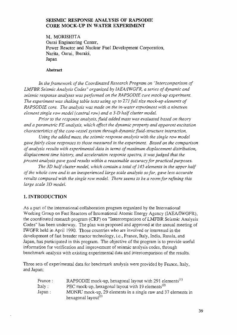
The core mock-up of RAPSODIE is presented in Fig. 2. It is composed of 91 fuelsubassemblies located at the center of the mock-up (one central subassembly and five rings)surrounded by 180 neutronic shield elements (four rings). A fuel subassembly is constituted

NEUTRONICSHIELDELEMENTS

FUELASSEMBLIES

Fig. 2 Experimental Set up of PEC Mock-up Core

15

of a cylindrical spike inserted to the diagrid and a hexcan containing the pin bundle. Aneutronic shield is constituted of a steel cylinder bolted on the dummy diagrid. The mock-upis surrounded by a stiff cylindrical vessel to perform tests in water. The vessel is assumed tobe rigid enough to induce no amplification of the table motion in the seismic frequency range.

For the seismic tests, the mock-up RAPSODIE was placed on the VESUVE shaking tablelocated at CEA/DMT at Saclay. Horizontal seismic excitation was ID and applied along thediameter of the mock-up. As benchmark problems, two sets of test data (one in air and theother in water) were provided in the form of time history response displacements at the top ofeach subassemblies, along with the table acceleration.

The natural frequencies and damping factors were given for each subassembly both for in-airand in-water. Shock stiffness value for the pad was also given.

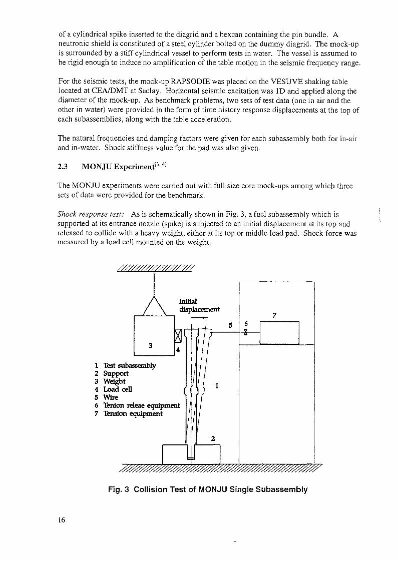
2.3 MONJU Experiment13 4]

The MONJU experiments were carried out with full size core mock-ups among which threesets of data were provided for the benchmark.

Shock response test: As is schematically shown in Fig. 3, a fuel subassembly which issupported at its entrance nozzle (spike) is subjected to an initial displacement at its top andreleased to collide with a heavy weight, either at its top or middle load pad. Shock force wasmeasured by a load cell mounted on the weight.

Initialdisplacement

1 lest subassembly2 Support3 Weight4 Load cell5 Wire6 Tenion releae equipment7 Tension equipment

Fig. 3 Collision Test of MONJU Single Subassembly

16

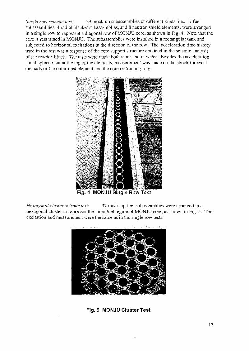
Single row seismic test: 29 mock-up subassemblies of different kinds, i.e., 17 fuelsubassemblies, 4 radial blanket subassemblies, and 8 neutron shield elements, were arrangedin a single row to represent a diagonal row of MONJU core, as shown in Fig. 4. Note that thecore is restrained in MONJU. The subassemblies were installed in a rectangular tank andsubjected to horizontal excitations in the direction of the row. The acceleration time historyused in the test was a response of the core support structure obtained in the seismic analysisof the reactor-block. The tests were made both in air and in water. Besides the accelerationand displacement at the top of the elements, measurement was made on the shock forces atthe pads of the outermost element and the core restraining ring.

Fig. 4 MONJU Single Row Test

Hexagonal cluster seismic test: 37 mock-up fuel subassemblies were arranged in ahexagonal cluster to represent the inner fuel region of MONJU core, as shown in Fig. 5. Theexcitation and measurement were the same as in the single row tests.

Fig. 5 MONJU Cluster Test

17

3. CALCULATION BY FINAS CODE

3.1 General Description of Analysis Method by FINAS Code

FINAS is a general purpose structural analysis system based on the finite element method. Ithas been developed by PNC since 1976, with a purpose of supporting overall structuraldesign and safety evaluation of FBR components. Its analytical capability includes staticstress, dynamic, and heat transfer analysis151.

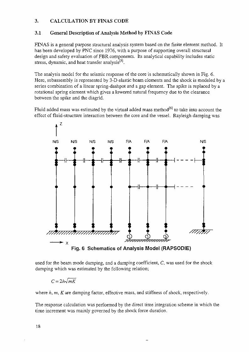
The analysis model for the seismic response of the core is schematically shown in Fig. 6.Here, subassembly is represented by 3-D elastic beam elements and the shock is modeled by aseries combination of a linear spring-dashpot and a gap element. The spike is replaced by arotational spring element which gives a lowered natural frequency due to the clearancebetween the spike and the diagrid.

Fluid added mass was estimated by the virtual added mass method16-1 to take into account theeffect of fluid-structure interaction between the core and the vessel. Rayleigh damping was

tN/S N/S N/S N/S F/A F/A F/A

///7//////J^//////7//////J^//

Fig. 6 Schematics of Analysis Model (RAPSODIE)

used for the beam mode damping, and a damping coefficient, C, was used for the shockdamping which was estimated by the following relation;

C - 2 Wm£

where h, m, K arc. damping factor, effective mass, and stiffness of shock, respectively.

The response calculation was performed by the direct time integration scheme in which thetime increment was mainly governed by the shock force duration.

18

3.2 Analysis on PEC Experiment1[7]

For the analysis on the PEC seismic experiment, two models, e.g., a five element single rowmodel and a twelve element half cluster model, were used. Since the natural frequency anddamping were not explicitly given in the problem, they were evaluated from the randomexcitation test results and the models were tuned to give these values.

In Fig. 7 compared are the distributions of the maximum displacements at the top of theelements on the central row. It is noted from the figure the distribution is rather even and thatthe analyses give somewhat larger displacements than the experiment. The half cluster modelgives slightly smaller displacements than the single row model, which seems to be reasonablesince in the half cluster model, some portion of the input energy is used for the out-of-planeresponse. Time history traces of the displacement response at the top of the central element(AO) on the central row are compared in Fig. 8. Although the maximum values are different,the appearances of the time histories are quite similar. From this resemblance, the presentanalysis can be judged to represent appropriate dynamic characteristics of the mock-up.Better response values are expected with a reduction in the apparent excitation due to thevessel-core interaction, which is not taken into account in the present calculations. Fig. 9 isthe distribution of the maximum shock forces. It is also quite even, and the two analysesgive consistent values.

b

,[BlJ(AlJ(AOJ[A4j[B7j

-o- 12Eim Analysis-c^SBm Analysis-X- Experiment

B1 A1 AO

Element NoA4 B7

Fig. 7 Comparison of Maximum Displacements: PEC

19

— 6

CL.t/JO

-3

-6

TOP OF AO, EXPERIMENT

2 T I M E (sec) 3

E

LUSLUO

CL°2Q

-3

-6

TOP OF AO, ANALYSIS (12 Elm)

T I M E (sec) 3

UJ

LUO

CL.ÇOO

-3

-6

TOP OF AO, ANALYSIS (5 Elm)

0 1 2 TI M E (sec) 3

Fig. 8 Comparison of Displacement Time histories: PEC

300

B1-A1 A1-AO AO-A4SHOCK LOCATION

A4-B7

Fig. 9 Comparison of Shock Forces between Analysis: PEC

20

3.3 Analysis on RAPSODIE Experiment

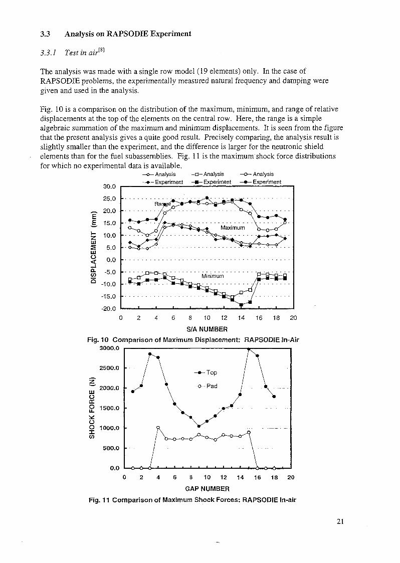
3.3.1 Testinairm

The analysis was made with a single row model (19 elements) only. In the case ofRAPSODIE problems, the experimentally measured natural frequency and damping weregiven and used in the analysis.

Fig. 10 is a comparison on the distribution of the maximum, minimum, and range of relativedisplacements at the top of the elements on the central row. Here, the range is a simplealgebraic summation of the maximum and minimum displacements. It is seen from the figurethat the present analysis gives a quite good result. Precisely comparing, the analysis result isslightly smaller than the experiment, and the difference is larger for the neutronic shieldelements than for the fuel subassemblies. Fig. 11 is the maximum shock force distributionsfor which no experimental data is available.

—o— Analysis -a— Analysis —o— Analysis—•»— Experiment —•— Experiment —•— Experiment

UJSUJO

0.CoQ

30.0

25.0

20.0

15.0

10.0

5.0

0.0

-5.0

-10.0

-15.0

-20.00 2 4 6 8 10 12 14 16 18 20

S/A NUMBERFig. 10 Comparison of Maximum Displacement: RAPSODIE In-Air

3000.0

2500.0

*"" 2000.0UJÜcc2 1500.0

oo 1000.0CO

500.0

0.00 2 4 6 8 10 12 14 16 18 20

GAP NUMBERFig. 11 Comparison of Maximum Shock Forces: RAPSODIE In-air

21

In Figs. 12 and 13 compared are the displacement time histories and the response spectra ofthe central fuel assembly (DC 10) on the central row. Quite good agreements can be seenbetween the analysis and experiment both for the time history and the response spectra.

From these observations, the present analysis is judged to give good results within a practicalaccuracy.

16

aiÜ 0o3 -8CL.CO5-16

0

DC10/Analysis

0.5

t t i i i J

1 1.5

TIME (sec)

2.5

DC10/Experiment

0 0.5 1 1.5 2

TIME (sec)

Fig. 12 Comparison of Displacement time Histories: RAPSODIE In-air

2.5

1200

cvS 900tn

RAPSODE IN WATER, CENTER ELM ON CENTRAL ROW

Z

600CCLUUJoq 300

0

DC10

M.

h=0.03— --ANALYSIS— -EXPERIMENT

0.01 0.1 PERIOD (sec) 1

Fig. 13 Comparison of Floor Response Spectra: RAPSODIE, In-air

22

3.3.2 Test in waterm

On the test in water, a single row and a 3D half cluster models were both used for theanalysis. The latter model, including 145 subassemblies, was a quite large scale andchallenging as a non-linear time response analysis. Before the response analysis, apreliminary study was made on the effect of fluid-structure interaction. The reductions innatural frequency and apparent (effective) excitation level were quantified by the study andused in the response analyses.

Fig. 14 is a comparison of the maximum and minimum displacement distributions along thecentral row. While the single row model gives a good agreement with the experimental data,the results of 3D half cluster model is somewhat larger than the others, especially in theminimum displacements. The reason for this unsymmetry in the half cluster analysis ispresently unknown. The distribution of the maximum shock forces are shown in Fig. 15. The3D half cluster analysis gives quite larger values than the single row model, which isconsistent with the displacement results.

RAPSODIE IN-WATER, CENTRAL ROW15.0

10.0

0.0

-15.0

-20.0

- Half cluster analysis

- Single row analysis- Eexperiment

l i t

Fig,

#01 #03 #05 #07 #09 #11 #13 #15 #17 #19ELEMENT NUMBER

14 Comparison of Maximum Displacement: RAPSODIE IN-WATER

8000RAPSODIE IN-WATER, CENTRAL ROW

z 6000 -LUOce2*:üOto

TOP, Half clusterTOP, Single rowPAD, Half clusterPAO, Single row

4000

2000 - -/- - -

ELEMENT NUMBER

Fig. 15 Comparison ot Maximum Shock Forces: RAPSODIE IN-WATER

23

In Figs. 16 and 17 compared are the displacement time histories and the response spectra ofthe central fuel assembly (DC 10) on the central row. As far as the time histories areconcerned, there is a good similarity in their appearances. It is consistent that in the spectrathere is a clear peak in 0.08 sec (12.5 Hz) which is a predominant component in the excitationspectra.

20

.Si

-20

z 20

ü 10S f o< ,§.o.= -20

DCIO/Experiment

0.5 1 1.5

T I M E (sec)

DC10/Analysis by half-cluster model

2.5

0.5 1 1.5

T IME (sec)

2.5

zOI5LUü

O.

Q

Fig

20 r DC10/Analysis by single row model

JO! 0

-10

-200 0.5 1 1.5

T I M E (sec)2.5

16 Compariosn of Displacement Time Histories: RAPSODIE IN-WATER

RAPSODIE iN-WATER, CENTRAL ROW/CENTRAL ELM. h=0.031200

— — Analysis/Single row

— — Experiment

0.01 0.10 Period (sec) 1.00

Fig. 17 Compariosn of Floor Response Spectra: RAPSODIE IN-WATER

24

From these observations, the present analysis with the single row model is judged to be ingood accordance with the experiment, while the re is a room for refinement in the half clustermodel.

3.4 Analysis on MONJU Experiment™

3.4.1 Shock response analysis

Prior to the seismic response analysis, a series of free vibration analyses which corresponds tothe shock response tests in air was performed with a single subassembly. In Fig. 18 shownare the time histories of shock force pulse accompanied by the local deformation behavior ofthe subassembly due to the shock at load pads. In the case of M.L.P., a fairly good agreementis seen between the analysis and the experiment on the first shock force both in term of itspeak value and duration. The shock force reaches its peak at around 3 msec after the contactoccurred, while the deformation of the subassembly is much slower. This suggests that theshock force is mainly governed by a local deformation of the load pad. In the case of theT.L.P., whose stiffness is much higher than that of the M.L.P., the duration of the shock force

\\xio4 \

;» 0.0~-0.2£-0.4oU- n K

H- °'6

<£ — 0.8I -1.0

-1.2

_

r

i

i

I//!'/v i ** v y° ' MFW^r

\

I

j — .*"

- —— Experiment— = — Analysis

-0.3 0.3 0.9 1.5 2.1TIME (SEC)

2.7X10'2 -1.4-0.5 0.5 1.5 2.5 3.5

TIME (SEC)4.5 5.5 X10"2

(a) (b)Fig. 18 Shock Response of Single Assembly (a) T.L.P. (b) M.L.P.

is very short and almost no deformation takes place in the subassembly during the shock.Although the analysis agrees with the experiment in terms of the duration, it gives abouttwice as high peak values as that of the experiment.

3.4.2 Seismic response analysis

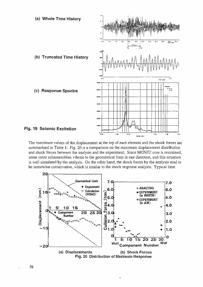
Among several experimental data provided, a seismic response analysis was made on the 29element single row experiment in air with 300 gal input. The time history trace and theresponse spectra of the input is shown in Fig 19 For the analysis, a portion of the timehistory starting at 9.0 sec and ending at 11.25 sec was used.

25

(a) Whole Time History

(b) Truncated Time History

(c) Response Spectra

Fig. 19 Seismic Excitation

The maximum values of the displacement at the top of each element and the shock forces aresummarized in Table 1. Fig. 20 is a comparison on the maximum displacement distributionand shock forces between the analysis and the experiment. Since MONJU core is restrained,some outer subassemblies vibrate to the geometrical limit in one direction, and this situationis well simulated by the analysis. On the other hand, the shock forces by the analysis tend tobe somewhat conservative, which is similar to the shock response analysis. Typical time

20, ——————————————————

^E 1 nl W

—c<D

1 0CD wu03aW

5-10

__O f\

x\ Geometrical Limits, ^ - ^"

00 x<x • Experiment

,0 °°0 , xx ° Calculation...°o°o0 m X (FiNAS)

°oooooo x

x

V* Component 20! 25l 30»h Number"W, 0°°0

>?00000000 °00X« o

X °n°oX °Xxx

X

XX

Nx

i .\J

Q t\j'-oÖl. ^ j C ^\^. o. v»

üj4.0Öl"13.0cOÜ2.0"o"1.0

0

«-ANALYSIS* EXPERIMENT

(in WATER)<* EXPERIMENT

(in AIR)

*.

** *JT

* ** *»«. * "

i i , »*i i i t

7.0

6.0

5 O.vr

4.0

3.0

2.0

1.0

n1 5i 101 15 20l 25i 30! w

Walll,, . .. . WallComponent Number

(a) Displacements (b) Shock ForcesFig. 20 Distribution of Maximum Response

26

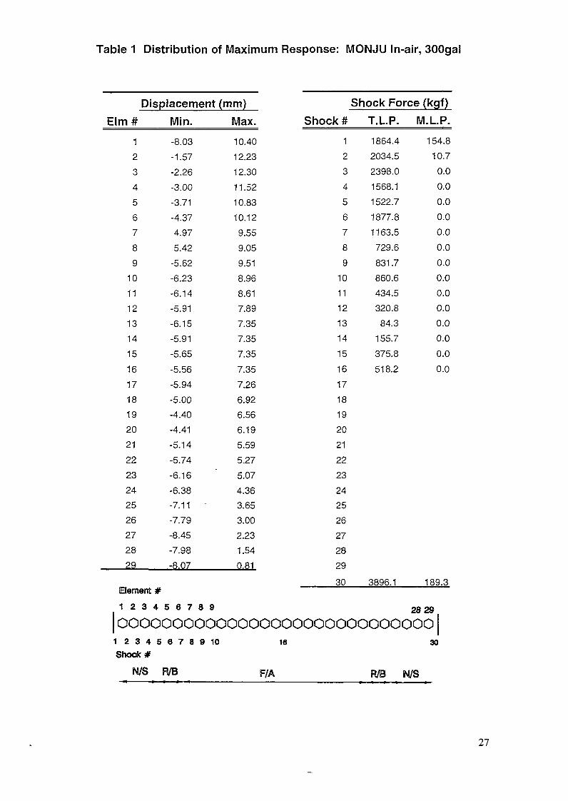
Table 1 Distribution of Maximum Response: MONJU In-air, SOOgal

Displacement (mm)Elm # Min.

1 -8.032 -1.57

3 -2.26

4 -3.00

5 -3.71

6 -4.37

7 4.97

8 5.42

9 -5.62

10 -6.2311 -6.1412 -5.91

13 -6.1514 -5.91

15 -5.6516 -5.5617 -5.9418 -5.0019 -4.40

20 -4.41

21 -5.1422 -5.7423 -6.1624 -6.3825 -7.1 126 -7.7927 -8.45

28 -7.98

29 -8.07

Bernent #1 2 3 4 5 6 7 8 9

oooooooooo1 2 3 4 5 6 7 8 9 1 0Shock #

N/S R/B

Max.

10.4012.2312.3011.5210.8310.12

9.55

9.059.518.968.617.89

7.35

7.357.35

7.357.266.926.56

6.19

5.59

5.275.074.363.653.002.23

1.54

0.81

Shock #1234

56

7

89

10

111213

14

15

16

17

18

19

20

21

22

23

24

25

26

27

28

29

30

Shock Force (kgf)T.L.P. M.L P.

1864.4 154.82034.5 10.72398.0 0.0

1568.1 0.01522.7 0.01877.8 0.01163.5 0.0729.6 0.0831.7 0.0860.6 0.0434.5 0.0320.8 0.0

84.3 0.0155.7 0.0

375.8 0.0518.2 0.0

3896.1 189.3

28 29

ooooooooooooooooooo16

F/A

30

R/B N/S

27

history traces of the response displacements at the top of the subassemblies are compared inFig. 21. Qualitatively, there is a good similarity between the analysis and the experiment.Fig. 22 is an overplot of the displacement time histories by the analysis which is given herefor the intercomparison purpose.

D1Analysis

Experiment

D7Analysis

Experiment

I !0'1 - 1

a.£ 0.«o

Fig. 21 Comparison of Displacement Time Histories

f

V

V

A

TOf -P I

10f_ -DZ

tor_ -03Tor -o<

I0f -D5

Toy -OBTOP -07

O.Z 0.5 1.0 ! • < 1.9 2

T I K E ( S E C )

F/fl . R/8 SNO N/5 39-600Ï I S E I S M t C HSVE 9-1 1 .25 J O t S P l f l C E H E N T

Fig. 22 Overplot of Displacement Response Time Histories: MONJU

28

4. INTERCOMPARISON OF ANALYSIS RESULTS

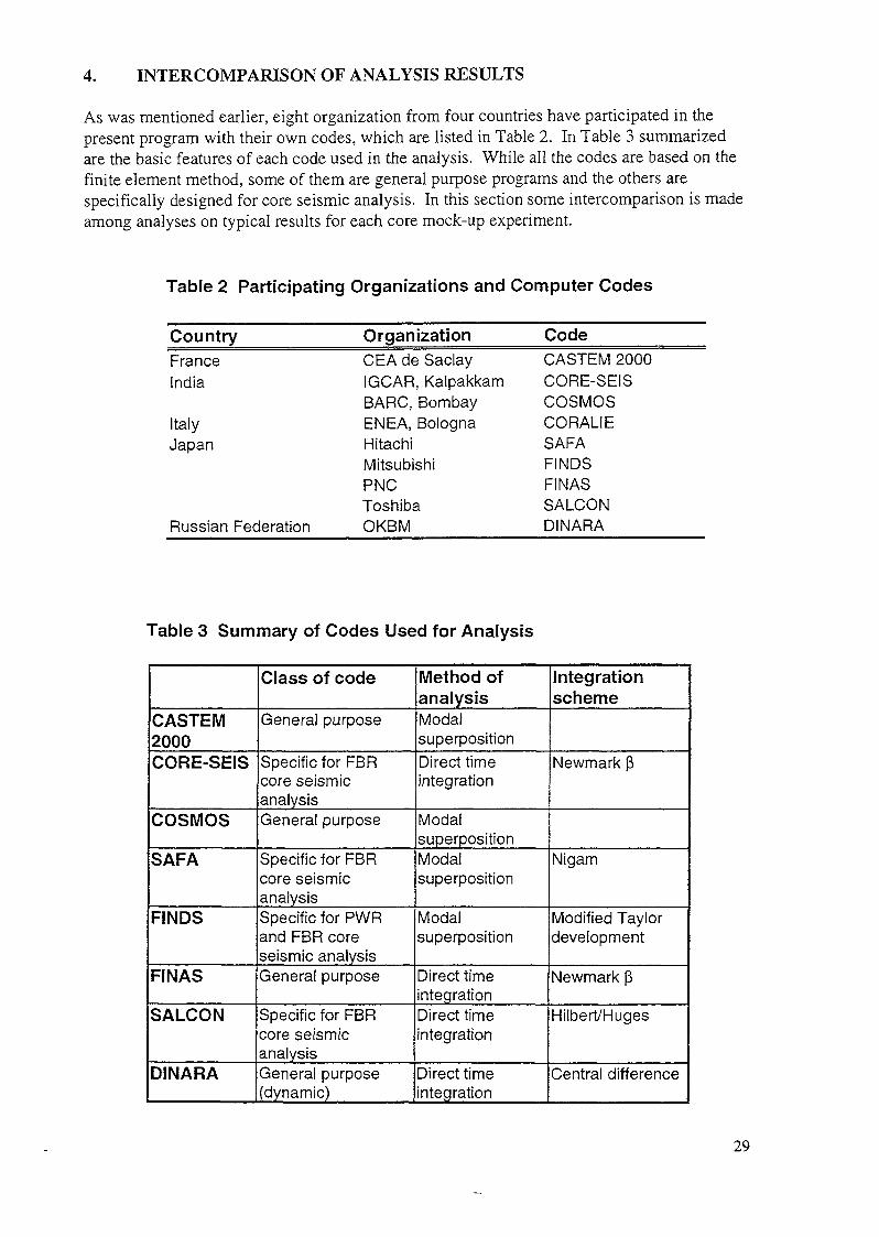
As was mentioned earlier, eight organization from four countries have participated in thepresent program with their own codes, which are listed in Table 2. In Table 3 summarizedare the basic features of each code used in the analysis. While all the codes are based on thefinite element method, some of them are general purpose programs and the others arespecifically designed for core seismic analysis. In this section some intercomparison is madeamong analyses on typical results for each core mock-up experiment.

Table 2 Participating Organizations and Computer Codes

CountryFranceIndia

ItalyJapan

Russian Federation

OrganizationCEA de SaclayIGCAR, KalpakkamBARC, BombayENEA, BolognaHitachiMitsubishiPNCToshibaOKBM

CodeCASTEM 2000CORE-SEISCOSMOSCORALIESAFAFINDSFIN ASSALCONDINARA

Table 3 Summary of Codes Used for Analysis

CASTEM2000CORE-SEIS

COSMOS

SAFA

FINDS

FINAS

SALCON

DINARA

Class of code

General purpose

Specific for FBRcore seismicanalysisGenera! purpose

Specific for FBRcore seismicanalysisSpecific for PWRand FBR coreseismic analysisGeneral purpose

Specific for FBRcore seismicanalysisGeneral purpose(dynamic)

Method ofanalysisModalsuperpositionDirect timeintegration

ModalsuperpositionModalsuperposition

Modalsuperposition

Direct timeintegrationDirect timeintegration

Direct timeintegration

Integrationscheme

Newmark ß

Nigam

Modified Taylordevelopment

Newmark ß

Hilbert/Huges

Central difference

29

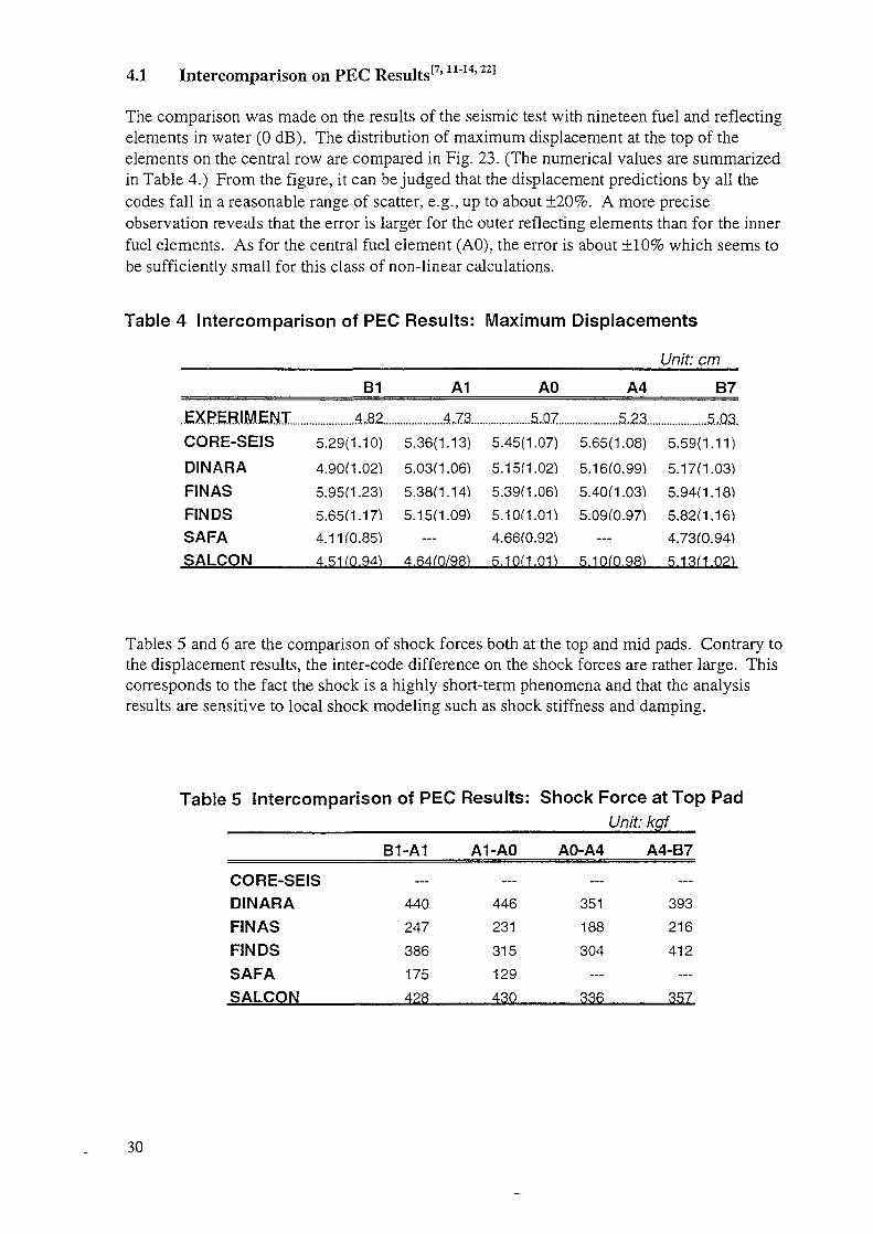
4.1 Intel-comparison on PEC Results17'n"14'22]

The comparison was made on the results of the seismic test with nineteen fuel and reflectingelements in water (0 dB). The distribution of maximum displacement at the top of theelements on the central row are compared in Fig. 23. (The numerical values are summarizedin Table 4.) From the figure, it can be judged that the displacement predictions by all thecodes fall in a reasonable range of scatter, e.g., up to about ±20%. A more preciseobservation reveals that the error is larger for the outer reflecting elements than for the innerfuel elements. As for the central fuel element (AO), the error is about ±10% which seems tobe sufficiently small for this class of non-linear calculations.

Table 4 Intercomparison of PEC Results: Maximum Displacements

EXPERIMENTCORE-SEISDINARAFINASFINDSSAFASALCON

B1

4,825.29(1.10)

4.90(1.02)5.95(1.23)5.65(1.17)

4.11(0.85)

4.51(0.94)

A1

4,735.36(1.13)

5.03(1.06)5.38(1.14)5.15(1.09)

—4.64(0/98)

AO

5,075.45(1.07)

5.15(1.02)5.39(1.06)5.10(1.01)4.66(0.92)

5.10(1.01)

A4

5,235.65(1.08)

5.16(0.99)5.40(1.03)5.09(0.97)

—

5.10(0.98)

Unit: cm

B7

5,035.59(1.11)

5.17(1.03)5.94(1.18)5.82(1.16)4.73(0.94)

5.13(1.02)

Tables 5 and 6 are the comparison of shock forces both at the top and mid pads. Contrary tothe displacement results, the inter-code difference on the shock forces are rather large. Thiscorresponds to the fact the shock is a highly short-term phenomena and that the analysisresults are sensitive to local shock modeling such as shock stiffness and damping.

Table 5 Intercomparison of PEC Results: Shock Force at Top Pad_____________________________Unit: kgf

B1-A1 A1-AO AO-A4 A4-B7

CORE-SEISDINARA 440 446 351 393FINAS 247 231 188 216FINDS 386 315 304 412SAFA 175 129SALCON__________428_____430_____336______357

30

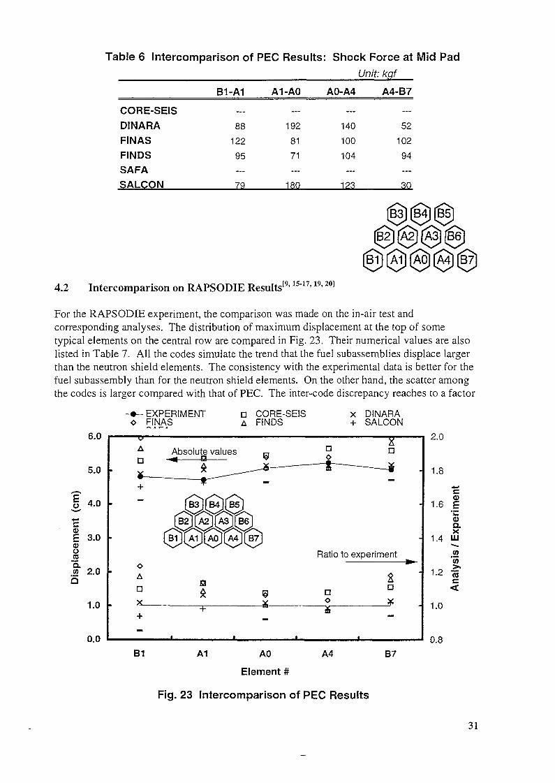
Table 6 Intercomparison of PEC Results: Shock Force at Mid PadUnit: kgf

CORE-SEISD1NARAF1NASFINDSSAFASALCON

B1-A1—88

12295—

79

A1-AO—

1928171—

180

AO-A4—

140100104

—

123

A4-B7—52

10294—

30

B1 A1 AO A4 B7

4.2 Intercomparison on RAPSODIE Results19'l5'17'19> 20]

For the RAPSODIE experiment, the comparison was made on the in-air test andcorresponding analyses. The distribution of maximum displacement at the top of sometypical elements on the central row are compared in Fig. 23. Their numerical values are alsolisted in Table 7. All the codes simulate the trend that the fuel subassemblies displace largerthan the neutron shield elements. The consistency with the experimental data is better for thefuel subassembly than for the neutron shield elements. On the other hand, the scatter amongthe codes is larger compared with that of PEC. The inter-code discrepancy reaches to a factor

I

eu0>

8Q.(A

6.0

5.0

4.0

3.0

2.0

1.0

0.0

-*- EXPERIMENTo FINAS

D CORE-SEISA FINDS

X DINARA+ SALCON

Ratio to experimentOAnx_

QX G

O

B1 A1 AO

Element #A4 B7

1.8

1.6

1.4

0)

0)CLX111CO

(g

1.0

0.8

Fig. 23 Intercomparison of PEC Results

31

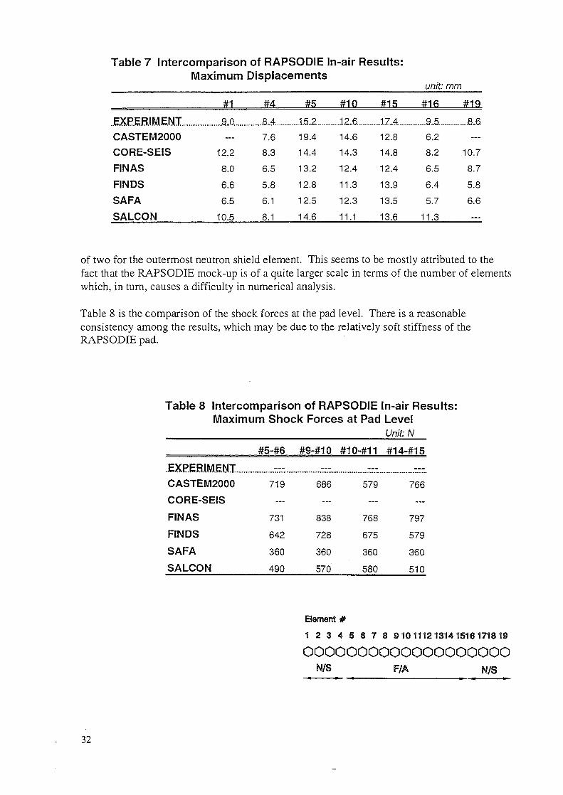
Table 7 Intercomparison of RAPSODIE In-air Results:Maximum Displacements

unit: mm

.EXPERIMENT.........CASTEM2000CORE-SEISFINASFINDSSAFASALCON

#1

9.0—

12.2

8.0

6.6

6.5

10.5

#4

8.47.6

8.3

6.5

5.8

6.1

8.1

#5

.......15.2......19.4

14.4

13.2

12.8

12.5

14.6

#10

.......12.6.......14.614.3

12.4

11.3

12.3

11.1

#15

.......17.4.......12.814.8

12.4

13.9

13.5

13.6

#16

..........9.5......6.2

8.2

6.5

6.4

5.7

11.3

#19

..........8.6.

10.7

8.7

5.8

6.6—

of two for the outermost neutron shield element. This seems to be mostly attributed to thefact that the RAPSODIE mock-up is of a quite larger scale in terms of the number of elementswhich, in turn, causes a difficulty in numerical analysis.

Table 8 is the comparison of the shock forces at the pad level. There is a reasonableconsistency among the results, which may be due to the relatively soft stiffness of theRAPSODIE pad.

Table 8 Intercomparison of RAPSODIE In-air Results:Maximum Shock Forces at Pad Level

_____________________________Unit: N

#5-#6 #9-#10 #1Q-#11 #14-#15

.JEXPEBIMENI....................---...................-CASTEM2000 719 686 579 766

CORE-SEISFINAS

FINDS

SAFA

SALCON

731

642

360

490

838

728

360

570

768

675

360

580

797

579

360

510

Bernent #1 2 3 4 5 S 7 8 9 10 1112 1314 1516 1718 19oooooooooooooooooooWS F/À N/S

32

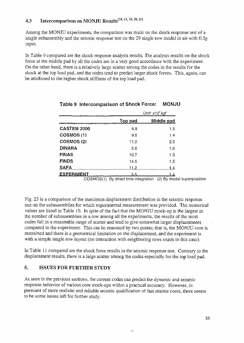
4.3 Intercomparison on MONJU Results"0'12> 18'20> 21]

Among the MONJU experiments, the comparison was made on the shock response test of asingle subassembly and the seismic response test on the 29 single row model in air with 0.3ginput.

In Table 9 compared are the shock response analysis results. The analysis results on the shockforce at the middle pad by all the codes are in a very good accordance with the experiment.On the other hand, there is a relatively large scatter among the codes in the results for theshock at the top load pad, and the codes tend to predict larger shock forces. This, again, canbe attributed to the higher shock stiffness of the top load pad.

Table 9 Intercomparison of Shock Force: MONJUUnit:x1(fkgf

CASTEM 2000COSMOS mCOSMOS (2)DINARAFINASFINDS

.SAFA........................................EXPERIMENT

Top pad

6.99.5

11.05.6

10.714.5

11.2R.5

Middle pad1.51.4

2.51.61.31.51 414

COSMOS(1) By direct time integration (2) By modal superposition

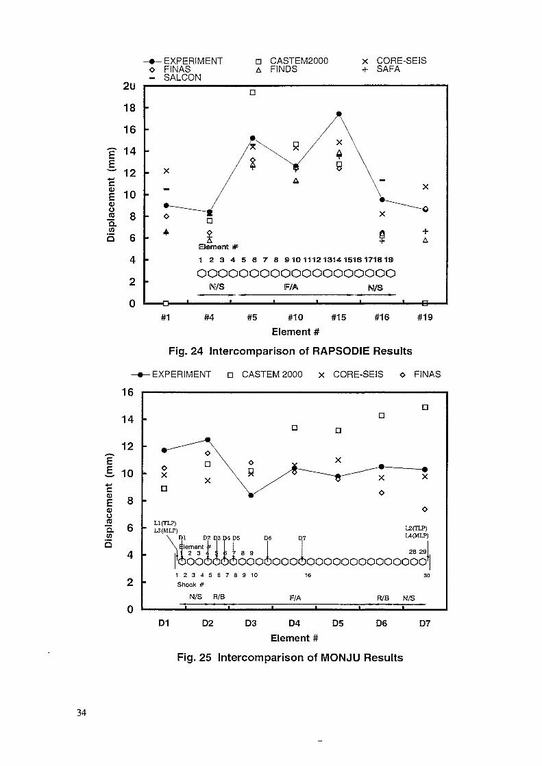
Fig. 25 is a comparison of the maximum displacement distribution in the seismic responsetest on the subassemblies for which experimental measurement was provided. The numericalvalues are listed in Table 10. In spite of the fact that the MONJU mock-up is the largest inthe number of subassemblies in a row among all the experiments, the results of the mostcodes fall in a reasonable range of scatter and tend to give somewhat larger displacementscompared to the experiment. This can be reasoned by two points; that is, the MONJU core isrestrained and there is a geometrical limitation on the displacement, and the experiment iswith a simple single row layout (no interaction with neighboring rows exists in this case).

In Table 11 compared are the shock force results in the seismic response test. Contrary to thedisplacement results, there is a large scatter among the codes especially for the top load pad.

5. ISSUES FOR FURTHER STUDY

As seen in the previous sections, the current codes can predict the dynamic and seismicresponse behavior of various core mock-ups within a practical accuracy. However, inpursuant of more realistic and reliable seismic qualification of fast reactor cores, there seemsto be some issues left for further study.

33

2U

18

16

-g 14

~ 124-«

I 10O)

8 8aV)5 6

4

2

0

16

14

12

I 10c0)

0)ÜJCCa.wa

8

2

0

-•- EXPERIMENTO FINAS- SALCON

D CASTEM2000A FINDS

X CORE-SEIS+ SAFA

Element1 2 3 4 5 6 7 8 9 10 1112 1314 1516 1718 19ooooooooooooooooooo

M/S F/A

#1 #4 #5 #10 #15

Element ##16 #19

Fig. 24 Intercomparison of RAPSODIE Results

EXPERIMENT D CASTEM 2000 X CORE-SEIS O FINAS

xD

L1(TLP)L3(MLP)

D6

8 9 TL2(TLP)L4(MLP)

28 29

oooôoooôoooooooooooooo'l1 2 3 4 5 6 7 8 9 1 0

Shock #

N/S R/B

16

F/A R/B N/S

D1 D2 D3 D4 D5Element #

D6 D7

Fig. 25 Intercomparison of MONJU Results

34

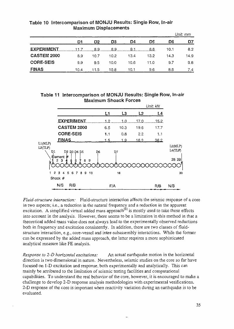
Table 10 Intel-comparison of MONJU Results: Single Row, In-airMaximum Displacements

Unit: mm

.EXPEBJMENZ..........CASTEM 2000CORE-SEISFINAS

D1

11.78.9

9.9

10.4

D2

8.910.7

9.5

11.5

D3

..........8.9. .......10.2

10.0

10.8

D4

9,113.4

10.6

10.1

D5

8.613.2

11.0

9.6

D6

10.1

14.3

9.7

8.6

D7

8.2

14.9

9.8

7.4

Table 11 Intercomparison of MONJU Results: Single Row, In-airMaximum Shoack Forces

Unit: kN

L1 L3 L2 L4

CASTEM 2000CORE-SEISFINAS

Ll(MLP)L3(TLP)

N1 Dilement •

2 3 '

bood

2 E¥. «

X

31

X

j>4

ï

bd

)5 I

r 8 9

boood

6.5

1.1

1.5

6 D

i)cooc

10.3 19.6 17.7

0.8 2.2 1.11.9 18.3 38.2

L2(MLP)7 L4(TLP)

28 29

boooooooooooooo1

1 2 3 4 5 6 7 8 9 1 0

Shock #

N/S R/B

16 30

F/A R/B N/S

Fluid-structure interaction: Fluid-structure interaction affects the seismic response of a corein two aspects; i.e., a reduction in the natural frequency and a reduction in the apparentexcitation. A simplified virtual added mass approach[6] is mostly used to take these effectsinto account in the analysis. However, there seems to be a limitation in this method in that atheoretical added mass value does not always lead to the experimentally observed reductionsboth in frequency and excitation consistently. In addition, there are two classes of fluid-structure interaction, e.g., core-vessel and inter-subassembly interactions. While the formercan be expressed by the added mass approach, the latter requires a more sophisticatedanalytical measure like FE analysis.

Response to 2-D horizontal excitations: An actual earthquake motion in the horizontaldirection is two dimensional in nature. Nevertheless, seismic studies on the core so far havefocused on 1-D excitation and response, both experimentally and analytically. This canmainly be attributed to the limitation of seismic testing facilities and computationalcapabilities. To understand the real behavior of the core, however, it is encouraged to make achallenge to develop 2-D response analysis methodologies with experimental verifications.2-D response of the core is important when reactivity variation during an earthquake is to beevaluated.

35

Response in a base isolated plant: Base isolation is a promising technology to enhanceseismic safety of an FBR. As its advantage is taken, the reactor block tends to be designedmore flexible both for reduction of thermal stresses and construction cost. An attentionshould be paid in this case to avoid frequency tuning between the reactor vessel and the core.In addition, there is little knowledge on the core response to displacement dominantexcitations which characterize the seismic isolation. Therefore, experimental and analyticalverification of the core under seismic isolation environment is desired.

Response to vertical excitations: Although it is unusual, when a very high level ofvertical excitation (diagrid response) is considered, up-lift, or floating, of subassemblies andconsequent loss of core configuration may become a concern. From the safety point of view,it is needed to establish qualification methods for the vertical response of the core.

Effect of pin bundles and bowing: In almost seismic response analyses it is assumedsubassemblies stand straight up at an even spacing, and that the effect of pin bundles on theflexural rigidity is negligible. In a high burn up core, there is a possibility that thermal andirradiation bowing of the subassemblies becomes significant and the pin bundles cannot beignored due to the bundle duct interaction (BDI). These factors can be dealt with by thecurrent analysis methods, and their effects on the seismic response may be studied.

6. CONCLUSIONS

As the final report on the Coordinated research Program on "Intercomparison of LMFBRSeismic Analysis Codes", the analysis results by FINAS on the PEC, RAPSODEE, andMONJU core mock-up experiments. Although these experiments vary in size, number ofsubassemblies, core configuration (free-standing or restrained), and excitation conditions, theresults by FINAS are in good accordance with the experimental data with a reasonableaccuracy. The present analysis method with FINAS, therefore, is judged to be capable forpractical use. However, there is still a room for improvement of analysis method, especiallyon large scale 3D problems.

Intercomparison of the results by the participants' code on some typical cases was showedthat they gave fairly close results for the PEC and MONJU experiments. For the RAPSODIEexperiment, which is the largest scale in the number of subassemblies, the variation amongthe codes is relatively large.

Finally, some issues were identified to be further studied from the view point of core seismicmethodology improvement.

REFERENCES

[1] BROCHARD, D. and GANTENBEIN, F., "Proposed benchmark problem forIAEA/Coordinated research program on intercomparison of LMFBR seismic analysiscodes", July 1994

[2] MARTELLI, A., A letter to IAEA and its attachment, October 1991[3] IWATA, K. et.al., "Proposed benchmark problems for IAEA/IWGFR coordinated

research program on intercomparison of LMFBR seismic analysis codes", April 1992[4] MORISHITA, M., "Proposed benchmark problems for MONJU core mock-up

experiments", document distributed to the CRP participants, July 1992[5] FINAS Version 12.0 User's Manual, PNC TN9520 92-006, March 1993

36

[6] FRITZ, R.J., "The effect of liquids on the dynamic motions of immersed solids",Trans. A.S.M.E., Jour. Eng. Ind., February 1972, pp!67~173

[7] MORISHITA, M., "Seismic response analysis of PEC reactor core mock-up", Proc. of1st RCM on CRP, IAEA/IWGFR, November 1993, Vienna, Austria

[8] MORISHITA, M., "Seismic response analysis of RAPSODIE core mock-up in-airexperiment", Proc. of 2nd RCM on CRP, IAEA/IWGFR, September 1994, OEC/PNC,O-arai, Japan

[9] MORISHITA, M., "Seismic response analysis of RAPSODIE core mock-up in-waterexperiment", Proc. of 3rd RCM on CRP, IAEA/IWGFR, May 1995, ENEA, Bologna,Italy

[10] MORISHITA, M. and IWATA, K., "Seismic behavior of a free-standing core in alarge LMFBR", Nuc. Eng. Des. 140(1993) pp309-318

[11] KOBAYASHI, T., "Calculation of PEC test by SALCON code", Proc. of 1st RCM onCRP, IAEA/IWGFR, November 1993, Vienna, Austria

[12] HORIUCHI, T. and MOTOMIYA, T., "Seismic analysis for PEC reactor coreexperiments using the SAFA program", Proc. of 1st RCM on CRP, IAEA/IWGFR,November 1993, Vienna, Austria

[13] ITOH, K., "PEC core mock-up seismic analysis by FENDS code", Proc. of 1 st RCMon CRP, IAEA/IWGFR, November 1993, Vienna, Austria

[14] VAZE, K.K. and MURLI, B., "Stage-II calculations -analysis of Italian tests-", Proc.of 1st RCM on CRP, IAEA/IWGFR, November 1993, Vienna, Austria

[15] KOBAYASHI, T., "Calculation of PEC and RAPSODIE tests by SALCON Code",Proc. of 2nd RCM on CRP, IAEA/IWGFR, September 1994, OEC/PNC, O-arai,Japan

[ 16] HORIUCHI, T. and MOTOMIYA, T., "Seismic analysis for the FBR core mock-upRAPSODIE experiments using the SAFA program", Proc. of 2nd RCM on CRP,IAEA/IWGFR, September 1994, OEC/PNC, O-arai, Japan

[17] ITOH, K., et.al., "RAPSODIE core mock-up seismic analysis by FINDS code", Proc.of 2nd RCM on CRP, IAEA/IWGFR, September 1994, OEC/PNC, O-arai, Japan

[ 18] FONTAINE, B., "Seismic behavior of in air MONJU core mock-up", Proc. of 2ndRCM on CRP, IAEA/IWGFR, September 1994, OEC/PNC, O-arai, Japan

[19] FONTAINE, B., "Seismic analysis of the FBR core mock-up RAPSODIE -CEAcalculation", Proc. of 2nd RCM on CRP, IAEA/IWGFR, September 1994, OEC/PNC,O-arai, Japan

[20] RAVI. R., et.al., Results of calculation with Japanese and French data by CORE-SEIS", Proc. of 2nd RCM on CRP, IAEA/IWGFR, September 1994, OEC/PNC, O-arai, Japan

[21] VAZE, K.K., et.al., "Co-ordinated research program on intercomparison of LMFBRseismic analysis codes -stage III-", Proc. of 2nd RCM on CRP, IAEA/IWGFR,September 1994, OEC/PNC, O-arai, Japan

[22] SELAEV, V.M., "Seismic response analysis of PEC reactor core mock-up byDENARA code", Proc. of 2nd RCM on CRP, IAEA/IWGFR, September 1994,OEC/PNC, O-arai, Japan

Next page(s) left blank

SEISMIC RESPONSE ANALYSIS OF RAPSODEECORE MOCK-UP IN WATER EXPERIMENT

M. MÖRISHITAOarai Engineering Center,Power Reactor and Nuclear Fuel Development Corporation,Narita, Oarai, Ibaraki,Japan

Abstract

In the framework of the Coordinated Research Program on "Inlercomparison ofLMFBR Seismic Analysis Codes" organized by IAEA/IWGFR, a series of dynamic andseismic response analyses was performed on the RAPSODIE core mock-up experiment.The experiment was shaking table tests using up to 271 full size mock-up elements ofRAPSODIE core. The analysis was made on the in-water experiment with a nineteenelement single row model (central row) and a 3-D half cluster model.

Prior to the response analysis, fluid added mass was evaluated based on theoryand a parametric FE analysis, which affect the dynamic property and apparent excitationcharacteristics of the core-vessel system through dynamic fluid-structure interaction.

Using the added mass, the seismic response analysis with the single row modelgave fairly close responses to those measured in the experiment. Based on the comparisonof analysis results with experimental data in terms of maximum displacement distribution,displacement time history, and acceleration response spectra, it was judged that thepresent analysis gave good results within a reasonable accuracy for practical purposes.

The 3D half cluster model, which contain a total of 145 elements in the upper halfof the whole core and is an inexperienced large scale analysis so far, gave less accurateresults compared with the single row model. There seems to be a room for refining thislarge scale 3D model.

1. INTRODUCTION

As a part of the international collaboration program organized by the InternationalWorking Group on Fast Reactors of International Atomic Energy Agency (IAEA/IWGFR),the coordinated research program (CRP) on "Intercomparison of LMFBR Seismic AnalysisCodes" has been underway. The plan was proposed and approved at the annual meeting ofIWGFR held in April 1990. Those countries who are involved or interested in thedevelopment of fast breeder reactor technology, i.e., France, Italy, India, Russia, andJapan, has participated in this program. The objective of the program is to provide usefulinformation for verification and improvement of seismic analysis codes, throughbenchmark analysis with existing experimental data and intercomparison of the results.

Three sets of experimental data for benchmark analysis were provided by France, Italy,and Japan;

France : RAPSODIE mock-up, hexagonal layout with 291 elements(1)

Italy : PEC mock-up, hexagonal layout with 19 elements(2)

Japan : MONJU mock-up, 29 elements in a single raw and 37 elements inhexagonal layout(3)

39

In this paper described are the results of preliminary and seismic response analysiscorresponding to the RAPSODIE in-water experimental data. The in-air experiment hasalready been analyzed in the previous paper{4). Analysis on the PEC and MONJU coremock-ups have already been reported also(5' \

2. PROBLEM DESCRIPTION0'

2.1 RAPSODIE CORE MOCK-UP

The core mock-up of RAPSODIE is presented in Fig. 1. It is composed of 91 fuelsubassemblies located at the center of the mock-up (one central subassembly and fiverings) surrounded by 180 neutronic shield subassemblies (four rings).

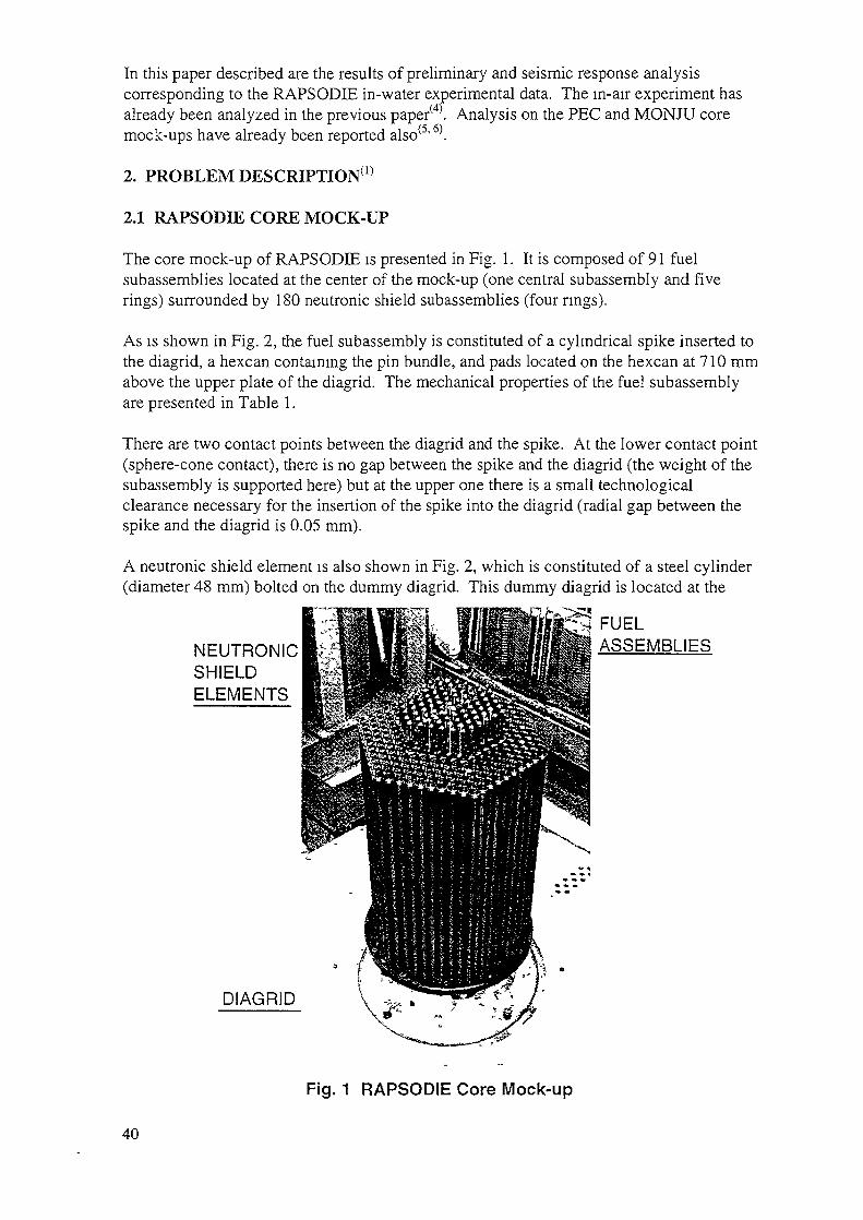
As is shown in Fig. 2, the fuel subassembly is constituted of a cylindrical spike inserted tothe diagrid, a hexcan containing the pin bundle, and pads located on the hexcan at 710 mmabove the upper plate of the diagrid. The mechanical properties of the fuel subassemblyare presented in Table 1.

There are two contact points between the diagrid and the spike. At the lower contact point(sphere-cone contact), there is no gap between the spike and the diagrid (the weight of thesubassembly is supported here) but at the upper one there is a small technologicalclearance necessary for the insertion of the spike into the diagrid (radial gap between thespike and the diagrid is 0.05 mm).

A neutronic shield element is also shown in Fig. 2, which is constituted of a steel cylinder(diameter 48 mm) bolted on the dummy diagrid. This dummy diagrid is located at the

FUELNEUTRONIC *£™»MHB««.ll«HBMMMHI ASSEMBLIESSHIELDELEMENTS

DIAGRID

Fig. 1 RAPSODIE Core Mock-up

40

50.8 mm 48

PAD

HEXCAN

DIAGRID '

y

S. ÎS" '

Fuel Assembly

1 »

Neutron Shield

Fig. 2 Fuel Assembly and Neutron Shield Element

Table 1 Mechanical Properties of Fuel Assembly

Elevation DensityTop Bottom(m) (m) (1E3 kg/m2 )

-0.240-0.0600.0000.0880.1201.2001.2521.2801.420

-0.0600.0000.0880.1201.2001.2521.2801.4201.500

7.87.8

19.0119.0189.87.87.87.87.8

Cross Sec.Area

(1E-6 m2)2516039531691691699531131

YoungsModulus(1E11 Pa)

1.91.91.91.91.91.91.91.91.9

BendingInertia

(1E-12m4)1360948254

256340559575595755957

2565401018

300000

same level as the diagrid upper plate. The mechanical properties of he neutronic shieldelement are presented in Table 2.

The bundle pitch of the whole mock-up is equal to 50.8 mm. The gaps separating thefaces of two adjacent subassemblies are summarized in Table 3. The mock-up issurrounded by a stiff cylindrical vessel (diameter : 1.1 m) in order to perform tests inwater. The vessel is assumed to be rigid enough in order to induce no amplification of thetable motion in the seismic frequency range.

41

Table 2 Mechanical Properties of Neutronic Shield

Elevation**Top(m)

0.0001 .280 *

Bottom(m)

1.2801.500

Density

(1E3 kg/m2)7.87.8

Cross Sec.Area

(1E-6 m2)2511

YoungsModulus(1E11 Pa)

1.91.9

BendingInertia

(1E-12m4)13609

300000These elements correspond to the link between the too of the subassernblies

and the displaecement transducersElevation 0.0 m corresponds to the upper plate of the diaqrid

Table 3 Gaps betweem Subassernblies

Asemblies

F/A - F/AF/A - N/SN/S - N/S

Gap at Pad Gap at Top(El 0.71m) (EL 1.28m)

0.1 11.5 0.72.8 0.4

Table 6 Fluid Added Mass

Node#

9876543

Elevation(m)

1.2801.2521.2000.7100.1200.0880.000

Added MassF/A

0.06300.18001.21952.43001 .39950.27000.1980

(kg)N/S0.06580.18801 .27372.53801.46170.28200.2068

unit : mm

2.2 SEISMIC TEST DATA

The seismic tests were carried out with the VESUVE shaking table located at CEA/DMTat Saclay. Since the detailed information on the experimental conditions has already beenreported(4), only the essential items pertinent to the analysis are simply repeated here;

Excitation: A 1-D horizontal seismic excitation applied along the diameter of themock-up, which was associated to a theoretical acceleration called '100% OBE'. Thetime history trace of the table acceleration and its response spectra are shown in Fig. 3. Tolimit the CPU time but in keeping a representative response, time duration for analysis was2.5 sec., beginning at the time 1.3 sec.

Natural Frequencies: The first natural frequency of a single subsubassembly are 8 Hz forthe fuel subassembly in air, 20 Hz for the neutronic shield element in air, and thefrequencies in water are 75% lower than those in air.

42

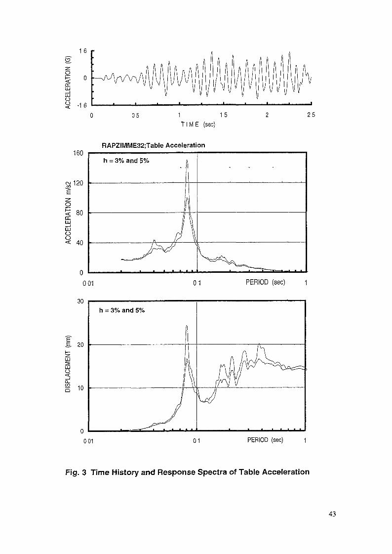
-n to" • CO ri <T> i M' r-t- o •2 0) 3 Q.

•33 (D (A TJ O 3 W ro W 73 (D a D) a B> ÇT ro > o o 2. o> 3 r+ 5' 3

DISP

LACE

MEN

T (m

m)

ACCE

LERA

TION

m/s

2CO o

-o m 2 O D

o CD

03 Oen o

ACCE

LERA

TION

(G)

en

o en

o m ;g O CD O

:r n co û) Q. tn

Jl > "O N m CO to 3 er (D > o o SL (D

ro cn

Impacts : The impacts between the subsubassemblies are supposed to take place atthe pad level and at the top. The local pad stiffness of the fuel subassemblies only is equalto 7.4xl(f N/m. For the other impacts between the subsubassemblies, they are supposed tobe very great.

Damping : The damping factors to be used in the calculations are 5% for all modes ofthe fuel subassemblies in water, 3% for all modes of the neutronic shield elements inwater.

3. CALCULATION OF FLUID ADDED MASS

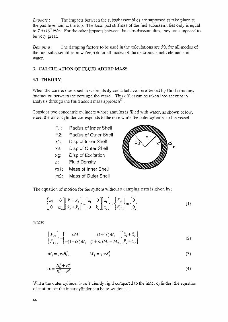
3.1 THEORY

When the core is immersed in water, its dynamic behavior is affected by fluid-structureinteraction between the core and the vessel. This effect can be taken into account inanalysis through the fluid added mass approach(7).

Consider two concentric cylinders whose annulus is filled with water, as shown below.Here, the inner cylinder corresponds to the core while the outer cylinder to the vessel.

R1 : Radius of Inner ShellR2: Radius of Outer Shellx1: Disp of Inner Shellx2: Disp of Outer Shellxg: Disp of Excitationp: Fluid Densityml: Mass of Inner Shellm2: Mass of Outer Shell

The equation of motion for the system without a damping term is given by;

m, 00 m,

k, 00 k2 J

(D

where

F,/2

M, =

CM, -(1 + cOMj

M2 =

(2)

(3)

a =FÇ-R? (4)

When the outer cylinder is sufficiently rigid compared to the inner cylinder, the equationof motion for the inner cylinder can be re-written as;

44

(m, + aMl )xl + k^ = -(/H, - M, )xg (5)

Thus, the reduction factors for the natural frequency, ßf, and the apparent excitation force,ße, are given by;

and

ße= ^"^i (7)

The discussion so far neglects the effect of inter-subassembly gap and the core is treated asa solid cylinder with the equivalent radius of R|. This effect was taken into account byTomita(8) by the following form.

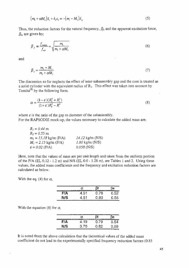
where £ is the ratio of the gap to diameter of the subassembly.For the RAPSODIE mock-up, the values necessary to calculate the added mass are;

RI = 0.44 mR2 = 0.55 mnu = 15. 18 kg/m (F/A) 14. 12 kg/m (N/S)M! =2. 1 5 kg/m (F/A) 1. 80 kg/m (N/S)£= 0.02 (F/A) 0. 055 (N/S)

Here, note that the values of mass are per unit length and taken from the uniform portionof the F/A (EL 0.12 - 1.2 m) and N/S (EL 0.0 - 1.28 m), see Tables 1 and 2. Using thesevalues, the added mass coefficients and the frequency and excitation reduction factors arecalculated as below.

With the eq. (4) for a,

a____ßf____ßeF/A 4.51 0.78 0.52N/S 4.51 0.80 0.55

With the equation (8) for a,

q ßf ßeF/A 4.19 0.79 0.54N/S 3.70 0.82 0.59

It is noted from the above calculation that the theoretical values of the added masscoefficient do not lead to the experimentally specified frequency reduction factors (0.85

45

for both F/A and N/S). This may mainly be attributed to the simplification of the realcore-vessel system to a set of ideal coaxial cylinders. The added mass coefficient tuned togive a frequency reduction by 0.85 can be derived from the eq. (6).

^1M,

x- (9)

The Values for this a are 2.71 for F/A and 3.01 for N/S, and the corresponding reductionfactors for the apparent excitation are 0.62 for F/A and 0.63 for N/S. The relation betweenthe added mass coefficient and the reduction factors are shown in Fig. 4.

1.0

0.9

o 0.8TJmLU

I 0.7•*—•o3

T3

tr 0.6

0.5

0.4

Frequency Reduction

- F/A, Theory(N/S)F/A, AnalysisN/S, Analysis

2 4 6

Added Mass Coefficient a

8

Fig. 4 Added Mass Coefficient and Frequency/Excitation Reduction

3.2 ANALYSIS

In order to ensure the validity of the theoretical added mass coefficients which were tunedto give lowered frequencies measured in the experiment, a parametric survey was madeboth on single F/A and N/S, using FINAS program. Here, the added mass for fluid wasattached to the nodes of EL 0.0 m through 1.28 m. From the results plotted in Fig. 4, theappropriate added mass (coefficients) are identified as 4.5 kgf/m (cc=2.1) and 4.7 kgf/m(cc=2.6), for F/A and N/S, respectively.

A small discrepancy is seen between the theory and analysis, which may come from thefact that in the theory a subsubassembly is simplified as a uniform beam while in theanalysis its mass and stiffness distribution along the axis is taken into account. In theresponse analysis, the added mass obtained by analysis to give experimentally measuredfrequencies, as identified above, will be used.

46

4. SEISMIC RESPONSE ANALYSIS

4.1 METHOD OF ANALYSIS

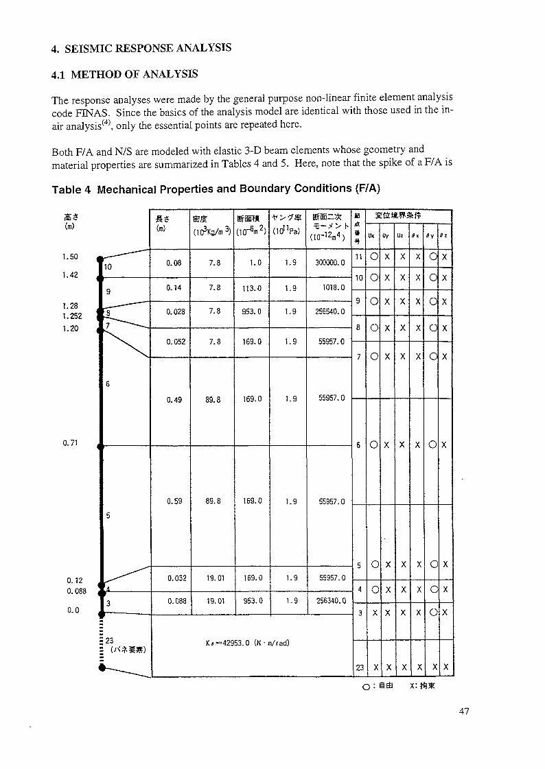
The response analyses were made by the general purpose non-linear finite element analysiscode FINAS. Since the basics of the analysis model are identical with those used in the in-air analysis{4), only the essential points are repeated here.

Both F/A and N/S are modeled with elastic 3-D beam elements whose geometry andmaterial properties are summarized in Tables 4 and 5. Here, note that the spike of a F/A is

Table 4 Mechanical Properties and Boundary Conditions (F/A)

(m)

1.50

1.42

1.281.2521.20

0.71

0.120.088

0.0

r -^"10

9

-—— — ——8

\6

5

^^

3

= 23

(m)

0.08

0.14

0.028

0.052

0.49

0.59

0.032

0.088

X.3,

7.8

7.8

7.8

7.8

89.8

89.8

19.01

19.01

ffirStt(10-V)

1.0

113.0

953.0

169.0

169.0

169.0

169.0

953.0

S£1.9

1.9

1.9

1.9

1.9

1.9

1.9

1.9

%-*>*(10-12m4)

300000.0

1018.0

256540. 0

55957.0

55957. 0

55957.0

55957. 0

256340.0

K «=42953.0 (N-m/rad)

H

»

11

10

9

8

7

6

5

4

3

23

3Ütti*#£f*

Ux

0

O

o

o

o

0

o

0

X

X

Uy

X

X

X

X

X

X

X

X

X

X

Uz

X

X

X

X

X

X

X

X

X

X

it

X

X

X

X

X

X

X

X

X

X

tfy

ooo

o

0

o

o

oo

X

Sz

X

X

X

X

X

X

X

X

X

X

o:

47

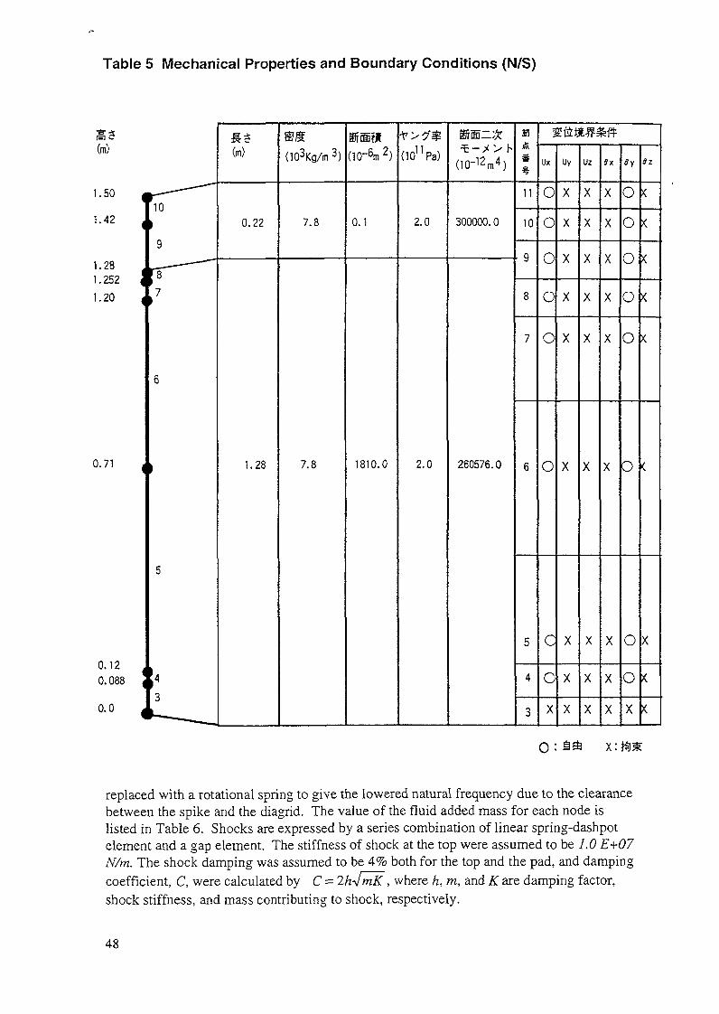
Table 5 Mechanical Properties and Boundary Conditions (N/S)

(m)

1.50

1.42

1.281.2521.20

0.71

0.120.088

0.0

10

9

H£(m)

0.22

1.28

ffiÄ(103Kg/m 3)

7.8

7.8

BBr®î«(10-6m2)

0.1

1810.0

V>?$(1011 Pa)

2.0

2.0

ÜB-Ä•Ï-» h

(10-12m4)

300000.0

260576. 0

Î3&9•*

11

10

9

8

7

6

5

4

3

£&##£#

Ux

oo

0

o

o

o

C

0

X

Uy

X

X

X

X

X

X

X

X

X

Uz

X

X

X

X

X

X

X

X

X

äx

X

X

X

X

X

X

X

X

X

«y

O

o

o

o

o

o

o

oX

Sz

<

<

<

X

<

(

X

X

<

0 :

replaced with a rotational spring to give the lowered natural frequency due to the clearancebetween the spike and the diagrid. The value of the fluid added mass for each node islisted in Table 6. Shocks are expressed by a series combination of linear spring-dashpotelement and a gap element. The stiffness of shock at the top were assumed to be 1.0 E+07N/m. The shock damping was assumed to be 4% both for the top and the pad, and dampingcoefficient, C, were calculated by C = Ih-JmK , where h, m, and K are damping factor,shock stiffness, and mass contributing to shock, respectively.

48

Two configurations, i.e., a single row (model A) and a 3-D half cluster model (model B),were used for the analysis. The former corresponds to the central row of the mock-up,while the latter to the upper half of the core. Schematic of the single row analysis model isshown in Fig. 5. In model B, the degrees of freedom out of excitation plane are allowedexcept for the elements on the central row (symmetry condition) and the shocks in theskewed direction between elements on two neighboring lines are taken into account.

tN/S N/S N/S N/S F/A F/A F/A N/S

Fig. 5 Schmatic of Single Row Analysis Model

Time history response was calculated by the direct integration method with time resolutionof 3.3E-5 sec (75900 steps). The results were written to disc in every 10 steps (3.3E-4 sec,7590 steps).

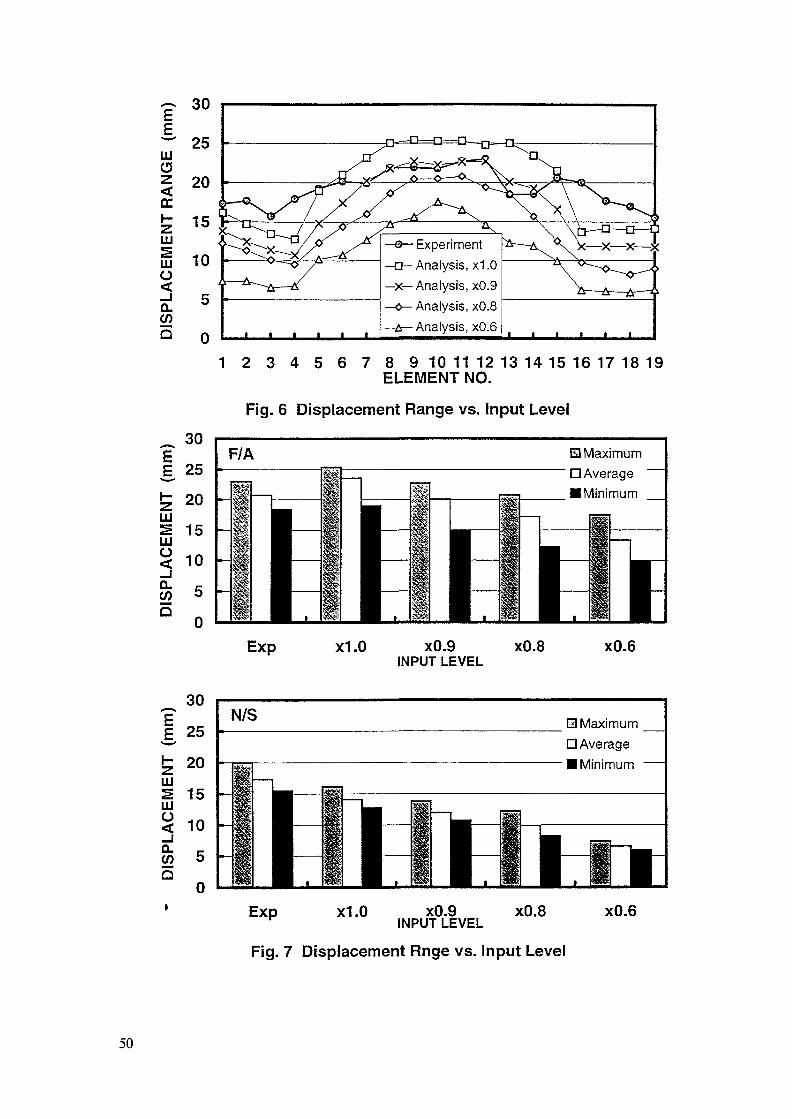
4.2 SURVEY ON EXCITATION LEVEL

The fluid-structure interaction between the core and the vessel not only affects the naturalfrequency of the subsubassemblies but also reduces the apparent excitation, as specified bythe eq.(7). Although a theoretical value for the excitation reduction factor can beestimated by this equation (about 0.5 ~ 0.6), it is uncertain whether this value gives aproper response result. Therefore a parametric survey was made to find an appropriateapparent excitation level which leads to the results close to the experimental data. Theexcitation level used were xl.O, xO.9, xO.8, andxO.6, of the original excitation data.

The distribution of the displacements range at the top of the subsubassemblies arecompared with those measured by the experiment in Fig. 6. The maximum, average, andminimum displacements among the F/A and N/S are compared with the experiment in Fig.7.

49

DISPLACEMENT (mm)

DISPLACEMENT (mm)

enro

ro

co

o

01

o

Ol

ro

ro

coo

in

o

T| v> "2. M O (D (D <Q fl> (A 5" T

J C

rn x TJ m<o

m r

x o * 00

m X TJ X b

TJ C m<£>

< m

x o oo X o CD

-n <5' o g w' o (D 3D D> D (£3 (D TJ r-f

(D

ro co £> Ol

O -4

me»

r~ gto m-j.

zo

H_i

z-1 PS _L CO _L 4^» _i 01 _1 O)

^4 00 CD

DIS

PLA

CE

ME

NT

RA

NG

E (

mm

)

O

01

O

O

lro

ro

co

o

01

o

H > >

> >

3

3

13

13

2L

Ë. SL

9L

•<

^<

><

><cfl

en

co

enw

' in

' w

' en

'X

X

X

X

P

P

P

r1cr>

bo

CD

As far as the F/A's are concerned, it can be judged that the apparent excitation which isreduced by 0.9 of the original data may give the closest response to the experiment. Onthe contrary, all of the analysis results on N/S's with various excitation level are smallerthan the experiment. This fact may suggest either some amplification occurred at theinstrumentation at the top of the N/S's, or that the damping factor of the N/S may be largerthan the value specified in the problem (5% of critical), since no amplification of the tableacceleration can be supposed.

Based on the above observation, the apparent excitation reduced by 0.9 was judged to bemost appropriate to use in the analysis to reproduce the experimental data. From theeq.(7), the value of added mass coefficient corresponding to this excitation reduction isabout zero (actually it is a small negative value which does not have a physical meaning).This means that as far as the excitation reduction is concerned the effect of the vessel-coreinteraction through fluid is negligible and the core can be treated as in infinite fluid.

4.3 RESULTS OF RESPONSE ANALYSIS

The numerical values of the maximum/minimum and the range of displacement responsesare summarized in Table 6.

The distribution of the maximum and minimum displacements in the X direction(excitation direction) at the top of the subsubassemblies (EL 1500 mm) are compared inFigs. 8 and 9 among the analyses and the experimental data, for the central and the 4throws, respectively. From Fig. 8, it is seen that the both analyses give response distributionfairly close to those from the experiment, as far as the maximum (positive) displacementresponses of F/A's are concerned. The single row model also gives response in thenegative direction which is close to those of the experiment. On the other hand, theminimum (negative) values of the half cluster model are rather larger than those from theexperiment and the single row model, and there seems to be an offset of about 5 mm forthe entire elements.

Since the neutron shield elements are much more stiff than the fuel subassemblies, themaximum displacement of the fuel subassemblies gradually decreases with increasingelement number (toward right hand side), due to the restraining effect of the neutron shieldelements. This tendency is well reproduced by the present analysis both for the maximumand minimum responses.

In Fig. 9 shown are the maximum and minimum displacement responses in the excitationdirection for the elements on the 4th row. For these elements on the off-center rows, thepresent (half cluster model) analysis gives somewhat larger values both in the maximumand minimum sides.

Figs. 10 and 11 are the distributions of maximum shock forces between neighboringelements on a same row at the top and the pad (shocks in the excitation direction). Theshocks on the central row are compared with those from the single row analysis. Theoverall tendency is reproduced by the analysis that the shock forces increase along theoutward direction with the maximum taking place between the outermost fuel subassemblyand the neutron shield element. However, the absolute values by the half cluster analysisare significantly larger than those by the single row analysis. This discrepancy may wellbe correlated to the fact that the present analysis gives larger displacements than the singlerow analysis.

51

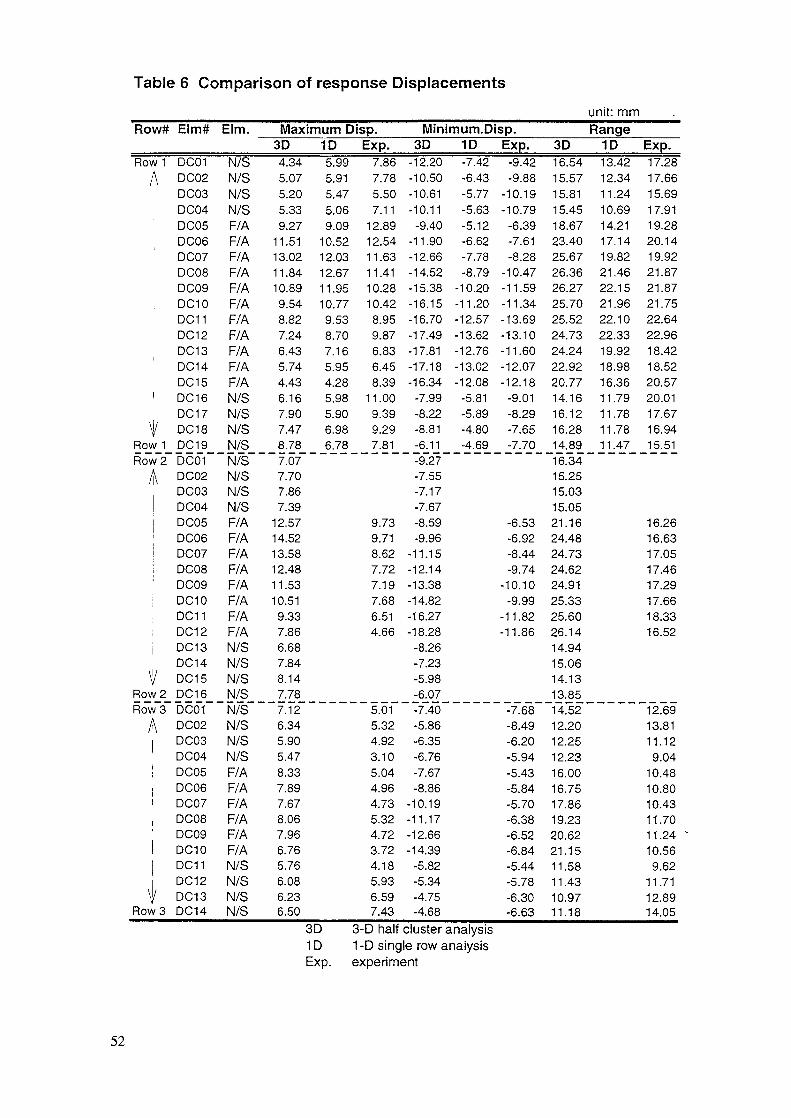
Table 6 Comparison of response Displacementsunit: mm

Row#

Row1A

VRow 1Row 2

A

VRow 2RowS

A

ii

VRowS

Elm#

DC01DC02DC03DC04DC05DC06DC07DC08DC09DC10DC11DC12DC13DC14DC15DC16DC17DC18DC19DC01DC02DC03DC04DC05DC06DC07DC08DC09DC10DC11DC12DC13DC14DC15DC16DC01DC02DC03DC04DC05DC06DC07DC08DC09DC10DC11DC12DC13DC14

Elm.

N/SN/SN/SN/SF/AF/AF/AF/AF/AF/AF/AF/AF/AF/AF/AN/SN/SN/SN/SN/SN/SN/SN/SF/AF/AF/AF/AF/AF/AF/AF/AN/SN/SN/SN/SN/SN/SN/SN/SF/AF/AF/AF/AF/AF/AN/SN/SN/SN/S

Maximum Disp.3D4.345.075.205.339.27

11.5113.0211.8410.89

9.548.827.246.435.744.436.167.907.478.787.077.707.867.39

12.5714.5213.5812.4811.5310.51

9.337.866.687.848.147.787.126.345.905.478.337.897.678.067.966.765.766.086.236.50

1D5.995.915.475.069.09

10.5212.0312.6711.9510.77

9.538.707.165.954.285.985.906.986.78

3D1DExp.

Exp.7.867.785.507.11

12.8912.5411.6311.4110.2810.42

8.959.876.836.458.39

11.009.399.297.81

9.739.718.627.727.197.686.514.66

5.015.324.923.105.044.964.735.324.723.724.185.936.597.43

3-D half

Minimum. Disp.3D

-12.20-10.50-10.61-10.11

-9.40-11.90-12.66-14.52-15.38-16.15-16.70-17.49-17.81-17.18-16.34

-7.99-8.22-8.81-6.11-9.27-7.55-7.17-7.67-8.59-9.96

-11.15-12.14-13.38-14.82-16.27-18.28

-8.26-7.23-5.98-6.07-7.40-5.86-6.35-6.76-7.67-8.86

-10.19-11.17-12.66-14.39

-5.82-5.34-4.75-4.68

cluster

1D-7.42-6.43-5.77-5.63-5.12-6.62-7.78-8.79

-10.20-11.20-12.57-13.62-12.76-13.02-12.08

-5.81-5.89-4.80-4.69

analysis

Exp.-9.42-9.88

-10.19-10.79

-6.39-7.61-8.28

-10.47-11.59-11.34-13.69-13.10-11.60-12.07-12.18

-9.01-8.29-7.65-7.70

-6.53-6.92-8.44-9.74

-10.10-9.99

-11.82-11.86

-7.68-8.49-6.20-5.94-5.43-5.84-5.70-6.38-6.52-6.84-5.44-5.78-6.30-6.63

Range3D16.5415.5715.8115.4518.6723.4025.6726.3626.2725.7025.5224.7324.2422.9220.7714.1616.1216.2814.8916.3415.2515.0315.0521.1624.4824.7324.6224.9125.3325.6026.1414.9415.0614.1313.8514.5212.2012.2512.2316.0016.7517.8619.2320.6221.1511.5811.4310.9711.18

1D13.4212.3411.2410.6914.2117.1419.8221.4622.1521.9622.1022.3319.9218.9816.3611.7911.7811.7811.47

Exp.17.2817.6615.6917.9119.2820.1419.9221.8721.8721.7522.6422.9618.4218.5220.5720.0117.6716.9415.51

16.2616.6317.0517.4617.2917.6618.3316.52

12.6913.8111.12

9.0410.4810.8010.4311.7011.2410.56

9.6211.7112.8914.05

1-D single row analysisexperiment

52

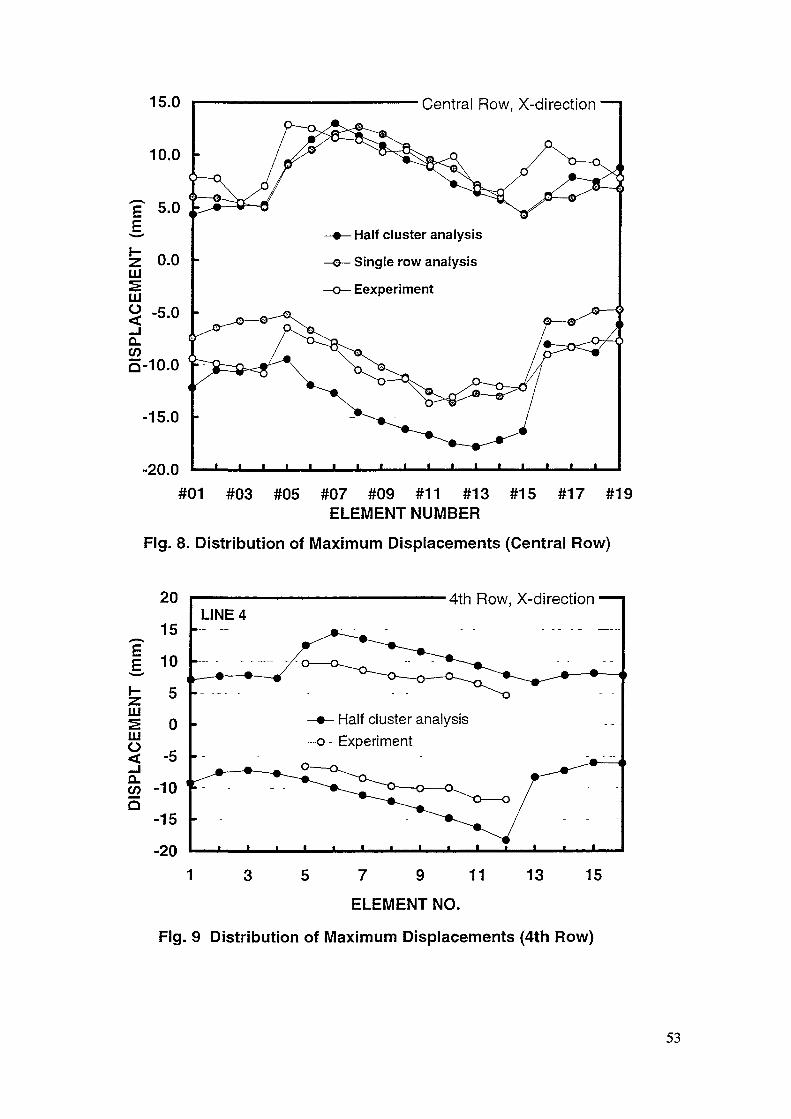
15.0

10.0

Central Row, X-direction

0.0LU

—•— Half cluster analysis

—©— Single row analysis

—o— Eexperiment

-20.0#01 #03 #05 #07 #09 #11 #13 #15 #17 #19

ELEMENT NUMBER

Fig. 8. Distribution of Maximum Displacements (Central Row)

£h-111LUÜ_Jo.

20

15

10

5

0

-5

-10

-15

-20

LINE 4• 4th Row, X-direction

Half cluster analysisExperiment

1 3 5 7 9 11 13 15

ELEMENT NO.

Fig. 9 Distribution of Maximum Displacements (4th Row)

53

80007000 -

g 5000ocg 4000

CENTRAL ROW.TOP, Half clusterTOP, Single rowPAD, Half clusterPAD, Single row

ELEMENT NUMBER

Fig. 10 Distribution of Maximum Shock Forces (Central Row)

5000

4000

LUO 3000GCOLL

OICO

2000

1000

•4th and 6th rows, Half cluster model analysis

—•—TOP, 4th row ~ ~~

CMOO=»:

Co

tOoino

00od>o

•a-CO

toT—

in

ELEMENT NUMBER

Fig. 11 Distribution of Maximum Shock Forces (Off-Center Rows)

54

Figs. 12 through 15 are the comparison of displacement time history traces at the top of theelements between experiment and two analyses. Here, the time history data for theexperiments are shifted in the time axis so that they fit with the analysis in light of overallwave form. Although there are some differences in the maximum values as describedabove, the appearance of the time history traces by the two analyses are similar to eachother. The resemblance of the time history traces between the analysis and the experimentis better for the fuel subassemblies than for the neutron shield elements, which is similar tothe maximum response values. Furthermore, the analysis on the central fuel subassemblyon the central row gives the best result among all. This corresponds to the fact theseelements are not allowed to displace in the out-of-plane d.o.f., and that shock force, whichmeans interaction of neighboring elements, is smaller in the center than in the outer regionof the core.

20

I 10t-aiS 0ü

ö! -1003Q

-20

E

tuSLUO

- Experiment

- v^

0.5 1 1.5T I M E (sec)

2.5

20

10

0

-10

-20

-Analysis by half-cluster model

0.5 1 1.5T IME (sec)

2.5

20 r Analysis by single row model

10LU

lü

CL

Q

-10

-20(

-•

5 0.5 1 1.5 2TIME (sec)

2.5

Fig. 12 Comparison of Displacement Response;Line 1/DC05/X-direction

55

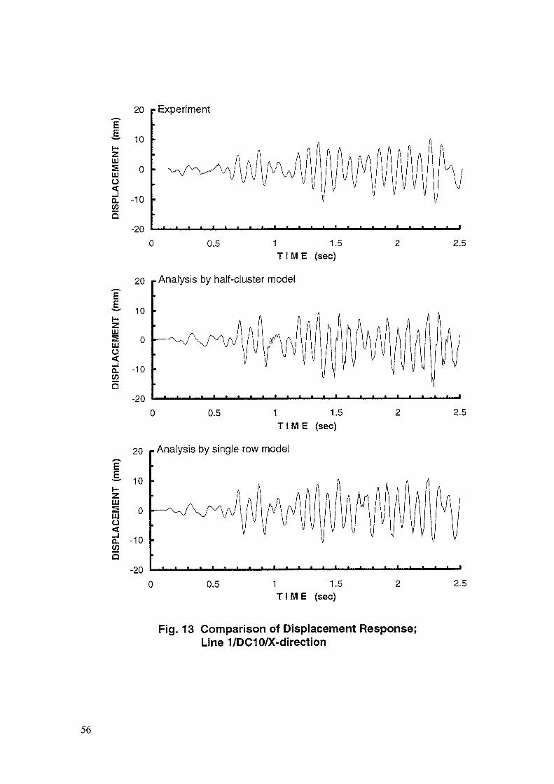
Os

DISPLACEMENT (mm)

DISP

LACE

MENT (mm)

DISP

LACE

MENT (mm)

ro oro o

ro oro o

ro o

•n cp* _i wr

o=

3ro

3-t

."O

öS.

O M

-••

OS

3 II ro u

38 ro ro i-t

- 33 ro (A TJ O (A ro

m •£• -

1s~'

en ro po en

co cr •< (D o 3 o Q.

(D

O Ü1

m W (D O

ro 01

E. *< ÇO w'

er •<O 01

c W s- -T l ^

—

S m (A (D O

ro ro 01

m x •a ro Z3 3' CD Zi

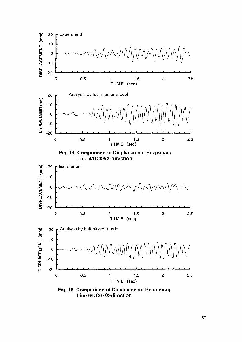
H-

LLISLUü

O.COa

E

O<Q.ÇOa

20

10

0

-10

-20

20

10

0

-10

-20

Experiment

0.5 1 1.5T I M E (sec)

2.5

Analysis by half-cluster model

0.5 1 1.5T I M E (sec)

E

aiSLUO

û.COQ

E

LUSLUü

20

10

0

-10

-20

Fig. 14 Comparison of Displacement Response;Line 4/DC08/X-direction

Experiment

o 0.5 1 1.5T I M E (sec)

20 p Analysis by half-cluster model

10

0

-100_COöö -20

0.5 1 1.5T I M E , (sec)

Fig. 15 Comparison of Displacement Response;Line 6/DC07/X-direction

2.5

2.5

2.5

57

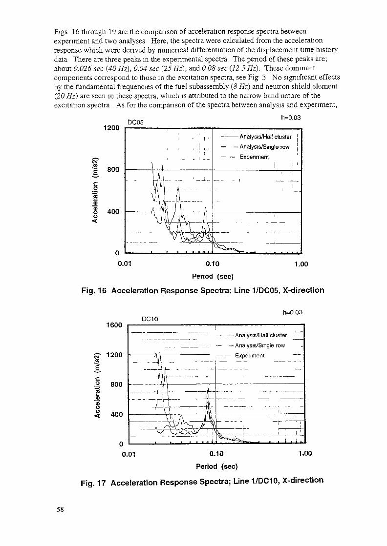
Figs 16 through 19 are the comparison of acceleration response spectra betweenexperiment and two analyses Here, the spectra were calculated from the accelerationresponse which were derived by numerical differentiation of the displacement time historydata There are three peaks m the experimental spectra The period of these peaks are;about 0.026 sec (40 Hz), 0.04 sec (25 Hz), and 0 08 sec (12 5 Hz). These dominantcomponents correspond to those in the excitation spectra, see Fig 3 No significant effectsby the fundamental frequencies of the fuel subassembly (5 Hz) and neutron shield element(20 Hz) are seen in these spectra, which is attributed to the narrow band nature of theexcitation spectra As for the comparison of the spectra between analysis and experiment,

1200

CM

•5 800

O

S 400ü

DC05h=0.03

- Analysis/Half cluster- Analysis/Single rowExperiment

0.01 1.000.10

Period (sec)

Fig. 16 Acceleration Response Spectra; Line 1/DC05, X-direction

OT

£

2Ji0)ou

1600

1200

800

400

DC10h=003

— —Analysis/Single row

— — Experiment

0.01 1.000.10

Period (sec)

Fig. 17 Acceleration Response Spectra; Line 1/DC10, X-direction

58

1200

CM

co°£!CC

0)

800

400

0.01 0.10 1.00Period (sec)

Fig. 18 Acceleration Response Spectra; Line 4/DC08, X-direction

1200

800

co"«3

o400

0.01 0.10 1.00Period (sec)

Fig. 19 Acceleration Response Spectra; Line5/DC07, X-direction

59

it is noted that the half cluster analysis gives somewhat lower peaks for the 5 Hzcomponent and larger peaks for the high frequency components.

5. CONCLUSIONS

As a part of the benchmark study in the framework of IAEA/IWGFR CoordinatedResearch Program on "Intercompariosn of LMFBR Seismic Analysis Codes", a series ofdynamic/seismic analyses was made on the French RAPSODIE core mock-up in-waterexperiment. The analyses were made by two models, i.e., the single row model and thehalf cluster model, after some preliminary work to find an appropriate values for the fluidadded mass.

The fluid added mass values were estimated based on the virtual added mass theory, andthe natural frequencies were first compared with the experimental values. Then using thesingle row model, added mass coefficient values were estimated to give maximumresponse displacements close to those by the experiment.

Using the above identified added mass coefficient, the response analyses by the twomodels were carried out and the results were compared with the experiment. It was foundthat the single row model gives a practically good result compared with the experiment,especially for the F/A's, while the accuracy of the half cluster model is somewhat lessgood. It seems to be a room for refining the half cluster model.

REFERENCES

(1) Brochard, D. and Gantenbein, F., 'Proposed Benchmark Problem for IAEACoordinated Research Program on Intercomparison of LMFBR Seismic AnalysisCodes Seismic Analysis of the FBR Core Mock-up RAPSODIE', July 1994

(2) Martelli, A., Letter from to IAEA and its attachments, October 1991(3) Iwata, K., et.al., 'Proposed Benchmark Problems for IAEA/IWGFR Coordinated

Research Program on Intercomparison of LMFBR Seismic Analysis Codes', PNCTN9410 92-004, April 1992

(4) Morishita, M., 'Seismic Response Analysis of RAPSODIE Core Mock-up In-airExperiment', Proc. of IAEA/IWGFR/RCM, September 1994, OEC/PNC, Japan,Austria, to be published.

(5) Morishita, M., 'Seismic Response Analysis of PEC Reactor Core Mock-up', Proc. ofIAEA/IWGFR/RCM, November 1993, Vienna, Austria, to be published.

(6) Morishita, M. and Iwata K., 'Seismic Behavior of a Free-standing Core in a LargeLMFBR', Nuc. Eng. Des., 140(1993), pp309-318

(7) Fritz, R.J., The Effect of Liquids on the Dynamic Motions of Immersed Solids',Trans. A.S.M.E., J. Eng. Ind., Feb. 1972, pp!67

(8) Tomita, H., 'Flow-path Network Model Analysis on Vibration Characteristics of aCluster of Rods in Fluid', Trans. J.S.M.E., C, Vol. 49, No.445. 1983 (in Japanese)

60

VERIFICATION AND VALIDATION ANALYSES ON LMFBRCORE MOCK-UP SEISMIC EXPERIMENTS BY FINDS CODE

K. ITOHMitsubishi Heavy Industries,YokohamaT. SATOH, I. AIZAWANuclear Development Corporation,Tokai-mura, IbarakiJapan

Abstract

The FINDS code which has capabilities of analyzing PWR,APWR and LMFBR cores deflection and colliding behaviors underseismic conditions has been applied to the LMFBR core mock-uptest data analyses to confirm the code capabilities to simulateLMFBR core seismic behaviors, performing the PEC, the RAPSODIEand the MONJU core mockup seismic analyses.

At first the PEC core seismic tests data were analyzed byusing the FINDS code to check the code capabilities to simulateLMFBR core seismic behaviors. Then it was confirmed that PECexperimental data are simulated fairly well by the FINDS codemodels.

The RAP087 AX01 wave test case in the air condition wasselected for the calculation of the RAPSODIE mockup tests where19 assemblies of one array were modeled. In addition theRAPZIMME32 wave test in the water condition was selected wherewhole assemblies composing the RAPSODIE three dimensional mockupwith 271 core assemblies of fuel assemblies and neutronic shieldelements are modeled in the FINDS calculations.

Then it was assured again that the RAPSODIE displacementsdata can be reproduced by the FINDS code models for both one rowand three dimensional cases, and three dimensional movements arerecognized by the graphical presentations in which some reducedresponse in three dimensional analysis appears because of shockforces dispersion effects in vertical direction compared with twodimensional behaviors, although slight discrepancy exists inneutronic shield elements displacements.

The Japanese prototype reactor MONJU mockup test data wereanalyzed for single assembly natural frequency and pad collisiontest data by the FINDS code, and the one array 29 assemblies testdata were analyzed by the general purpose code ANSYS. Theconsistencies were obtained in the ANSYS analyses both indisplacements and colliding forces between wapper pads.

Comparison with other codes calculations are summarizedconsidering the test accuracies because the tests results cannotbe traced now by the lack.of data.

Finally future tasks remained are discussed not only to getmore precise codes and but also to get design methodology forseismic events.1.Introduction

Much efforts have been offered in the Mitsubishi nuclearpower plant engineering sections to analyze core seismicbehaviors both in PWR, APWR and LMFBR plants designs. In PWR and

61

APWR core seismic analyses, time historical behaviors of fueldisplacements and colliding forces at grid spacers were directlycalculated by a computer code named "FUVIAN" from the early stageof its design. The FUVIAN code was successfully revised to theFINDS code by introducing grid spacers in-elastic analyses. TheFINDS code has not only the PWR and the APWR core analysiscapability but also can analyze LMFBR core seismic behaviorsincluding collisions at spacer-pads.

In this paper, the PEC, the RAPSODIE and the MONJU coresseismic tests data were analyzed by using the FINDS code to checkthe FINDS code capability to simulate LMFBR core seismicbehaviors.

2.Finds code models2.1 General Features of FINDS code

The Mitsubishi PWR core seismic analysis code FUVIAN hasbeen continuously advanced until the introduction of non-lineardamping models (FUVIAN4). The next stage of the developing workin the fuel seismic analysis was recognized to treat elasto-plastic impact behaviors of the fuel grids. After the task wassolved, the code is renamed to be the FINDS (Fuel IN-elasticDeformation under Seismic conditions) which has now thecapability to analyze not only PWRs and APWR cores but also LMFBRcores seismic behaviors, the latter model of which was formulatedby reflecting the experiences in Mitsubishi advanced reactordesign sections through the MONJU and the Japanese DFBR coreseismic design works.

The calculation model of the FINDS code for a PWR coreanalysis is shown in Fig.2-1. In order to describe the motion offuel subassemblies(F/As), the finite element methodology(FEM) isused where a F/A is treated as a combination of beams withdistributed masses and stiffness. Then a vibrational motions ofa F/A is described in the next forms.

Seara (F/A) No.1 2 3 ........ L

v•ao

:2

3

n

•o

!

3C

1 [

X

J l

3---- - G3--- - - c

J

3X

3

••••

• -*

~™

^— P.srrcl _^_

\Imp? er.

Elleocnt i— Equivalent i*'

Ecam

•777

^- Louer Core P la te

JLLL 8 .

^f~

•t

BTTT ^

X. ,l-t-1

Nodal DIsplacenent Seismic AccerelationTranslational

Rotational

F i g - 2 - 1 . Colliding Vibrations of F/As Calculation Model62

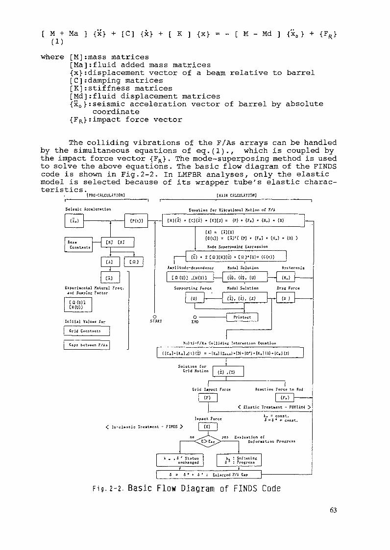
[ M + Ma ] {x> + [C] {x} + [ K ] {x> = - [ M - Md ] {x0 } + {FR}(1)

where [M] :mass matrices[Ma]:fluid added mass matrices{x} : displacement vector of a beam relative to barrel[C]:damping matrices[K] :stif fness matrices[Md]:fluid displacement matrices{x0 ]• : seismic acceleration vector of barrel by absolutecoordinate

: impact force vector

The colliding vibrations of the F/As arrays can be handledby the simultaneous equations of eq.(l)., which is coupled bythe impact force vector {FR}. The mode-superposing method is usedto solve the above equations. The basic flow diagram of the FINDScode is shown in Fig. 2-2. In LMFBR analyses, only the elasticmodel is selected because of its wrapper tube's elastic charac-teristics.

(PRE-CALCULATIOK] [KJUN CALCULATION]

Seiaslc Acceleration Equat ion for Yibraticnal Notion of F/A

fr i , , f r f r ï } . • r v f i r r i t r n f f \ • r r

Béa» —— [XJ £«

*Ç A ] c a }

*m

Eiperi«ental Katural Freq.and Daapinc Factor

tu (D)]tH(unC

Initial Values for ST

Grid Constants

Caps between F/As

w{6(t

Kod

](« = {P} * (F.) « {Hj * (0> —— |

= HHU))} = EÎ3T( {P) * (F,} « {H,} » (D) )

j ——— {0} * 2 C Q ] [ H ] ( U ) « [ Q 3 M U ) = (G(O>'

C O ( U ) D . L H ( U ) ]

Supportinc Force

(0} ——

1

> o ———AKT £«D

Hodal Solution Hystereaîa

—— (Ü) , (U) , (U) —— (H r) ———— -

Kodal Solution Drac Fore«

—— (X), (J), W -r- (0} —————

———————— 1

Hult i -F/As Collidinc Interaction Equation

( t C o l t U a l ^ O l Z ) = - ÎXo!(ZO L O )»[D!»{D' ï»{K.)(X!t[C,](X|

Grid Jiotioni

(i) ,{z>l

! !Grid Impact Force Reaction Force to Rod

< Elastic Treatment - FUYHM4 >

, _ t, = const.Upact Force ,B j . . consU

< In-elastic Treatment - FIfiOS > | {£) |

no ^^-^^v^^ yes Evalua t ion of

^\^-

k . , { ' Statusunchanced

+j J = o • » { ' : Z

k. : SoftenincS f : Procrcss

»Jilarted F/A Gap j ————————————————— '

F i g . 2-2. Basic Flow Diagram of FINDS Code63

The process to solve eq.(l) in the FINDS is describedbelow.

At first it is assumed that {X} can be expressed by thesuperposition of natural vibration modes as the next form.

{X} = [A]{u>where {U> = {ul,u2,,um}T

: Mode intensity vector (u. means instantaneous magnitude of i-th node)[A] = [A][B][A] = ((Al,, (A)., ........,{A] )T : • Mode matrix1 2 m •Î.AJ, : normalized i-th mode shape

^ '[Bj : m x ra diagonal matrix whose i-th element is

m : Max. mode number (m à 2n-2)Then assuming no interaction of damping between any two

modes, eq.(l) is converted to eq.(3). The equation for eachvibrational mode is connected each other only through theexternal force term {G(t)}.

W + 2[O.][HHu} + [a]2{u} = {G(t)> (3)where [£}] : natural angular frequency matrix, m x m

diagonal .[H] : damping factor (fraction of critical

dampingmatrix, m x m diagonal.

)> = [A]T (

2.2 Multi-F/As Colliding Interaction ModelIn order to solve the multi-F/As colliding interaction, one

transverse array of wrapper pads at the same elevation ismodeled. When the equilibrium of forces is consid-ered, the next equations are formulated.

where fj = (zj-!-zj-6j-ô?)k • + ( z- -z--^-^) c. . g j . J i J - I J ' g J 4fj+i: similar as above * 'frj = (zj-xpkr.-Kz cr.

zj : displacement of grid at joint jxj : displacement of rods at joint j

Taking the above eq.(4 ) into account, the equation for themulti-F/As interaction at a given wrapper pads elevation isobtained as follows.

[KG ]At) {z} --[KR] X +[C R ]{X}

64

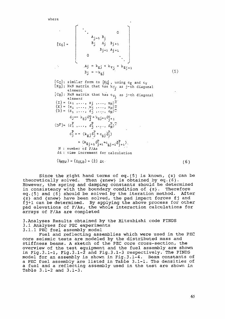
where

[KG] =3J AJ

•AJ = kgj + krj + k„.(5)

[CG]; similar form to [KG] , using cg and cr' ; NxN matrix that has kf.. as j-ch diagonal

element -; NxN matrix that has cr. as j-ch diagonalelement J

{Z} = (zi ,. . . , zj ,. .., ZN)T{X} = (xj. , ..., xj ,..., xN)T{D}= (d, ,..., dj ,..., dN)T

= (d? ,..., d? ,..., d^)

N : number of F/AsAt : time increment for calculation

At. (6)

Since the right hand terms of eq.(5) is known, {z} can betheoretically solved. Then {znew} is obtained by eq.(6).However, the spring and damping constants should be determinedin consistency with the boundary condition of {z}. Thereforeeq.(5) and (6) should be solved by the iteration method. After{z} and {znewj- have been solved, the pad impact forces f j andfj+1 can be determined. By applying the above process for otherpad elevations of F/As, the whole interaction calculations forarrays of F/As are completed3.Analyses Results obtained by the Mitsubishi code FINDS3.1 Analyses for PEC experiments3.1.1 PEC fuel assembly model

Fuel and reflecting assemblies which were used in the PECcore seismic tests are modeled by the distributed mass andstiffness beams. A sketch of the PEC core cross-section, theoverview of the test equipment and the fuel assembly are shownin Fig.3.1-1, Fig.3.1-2 and Fig.3.1-3 respectively. The FINDSmodel for an assembly is shown in Fig.3.1-4. Beam constants ofa PEC fuel assembly are listed in Table 3.1-1. The densities ofa fuel and a reflecting assembly used in the test are shown inTable 3.1-2 and 3.1-3.

65

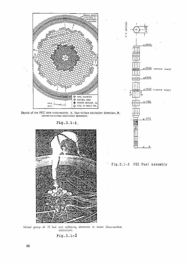
FUEL EUZXSWTSCOS'TOTt. SODSFORCîD X£?L£CT.FUEL tS DECAY ?OS.

Sketch of the PEC core cross-section. /4, face-to-face excitation direction;corner-to-corner excitation direction.

Fig.3.1-1,

. 3000

0

• 2S5S C u f > » E R J>A O S )

T2200

1 1 4 4 0 ( L O W E R PADS)

LUUy 7 100

372

Fig.3.1-3 PEC-Fuel assembly

Mixed group of 19 fue l and re f lec t ing elements in water (f;iee-to-faceexcitat ion).

Fig.3.1-2

66

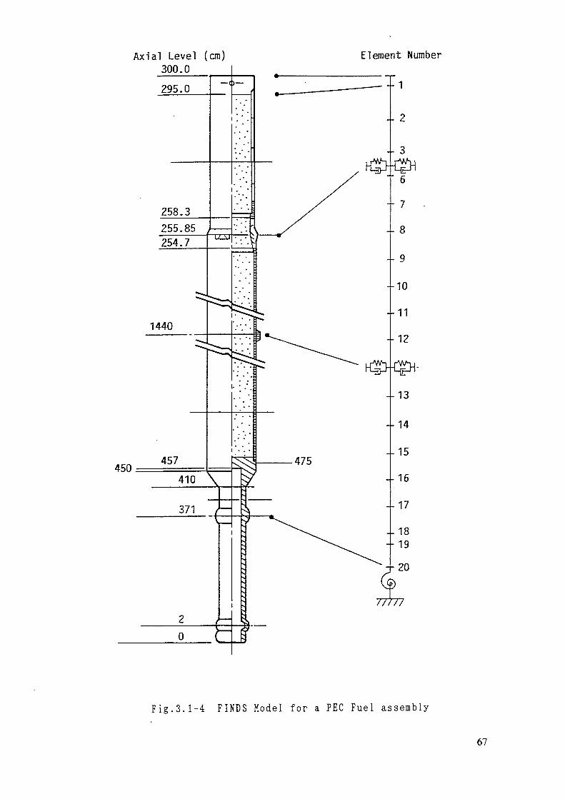
Axial Level (cm)300.0

450

Fig.3.1-4 FINDS Model for a PEC Fuel assembly

67

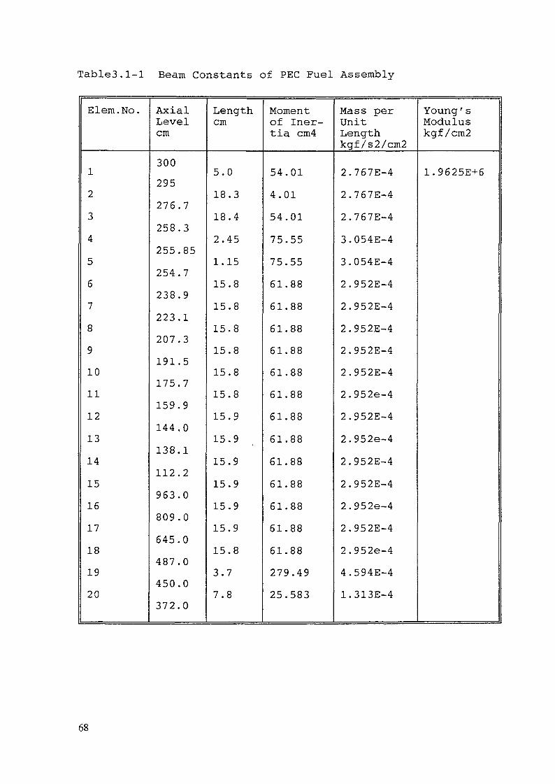
Table3.1-1 Beam Constants of PEC Fuel Assembly

Elem.No.

1234567891011121314151617181920

AxialLevelcm

300295276.7258.3255.85254.7238.9223.1207.3191.5175.7159.9144.0138.1112.2963.0809.0645.0487.0450.0372.0

Lengthcm

5.018.318.42.451.1515.815.815.815.815.815.815.915.915.915.915.915.915.83.77.8

Momentof Iner-tia cm4

54.014.0154.0175.5575.5561.8861.8861.8861.8861.8861.8861.8861.8861.8861.8861.8861.8861.88279.4925.583

Mass perUnitLengthkgf/s2/cm2

2.767E-42.767E-42.767E-43.054E-43.054E-42.952E-42.952E-42.952E-42.952E-42.952E-42.952e-42.952E-42.952e-42.952E-42.952E-42.952e-42.952E-42.952e-44.594E-41.313E-4

Young ' sModuluskgf /cm2

1.9625E+6

68

Table 3.1-2 Densities of Fuel Assembly of 19 Groups

Element Number12,34,56-181920

in Air8.1064.99165.5094.99548.1068.106

in Water3.5626.70967.2276.58749.2175.904

Table 3.1-3 Densities of Reflector Assembly of 19 Groups

Element Number12,34,56-181920

in Air8.1066.96207.15226.96348.1068.106

in Water3.5628.6808.8708.55549.2175.904

The damping constants for each mode is listed in Table 3.1-4. The same constants were used in this analyses for the reasonthat the damping characteristics were not clarified and thegeometries of the fuel assembly and the reflector are alike.

The natural frequencies of the PEC fuel and the reflectingassembly are modeled by the FINDS as shown in Table 3.1-5. Thenatural vibrational modes up to the third mode are drawn for thefuel assembly in Fig.3.1-5 and for the reflecting assembly inFig.3.1-6. The spike stiffness was defined by to fit the measureddata of the air condition changing the stiffness and theexcitation values which is shown in Fig.3.1-7.

The first modes are consistent between measured values andcalculation models. Higher modes cannot be checked because theywere not measured.

Table 3.1-4 Damping Constants of Beam Elements in Water(Reference Case)

Core AssemblyReflector

1st Mode5 %5 %

2nd Mode3 %3 %

3rd Mode3 %3 %

69

Table 3.1-5 Natural Frequencies

Core Fuel Assembly in Airin Water

ExperimentReflector Assembly in Air

in WaterExperiment

1stMode

3.58-3.25-3.23.04-3.17-3.25

2ndMode

26.9-24.4

22.9-22.1

3rdMode

80.5-73.0

68.4-64.8

MODE 1 MODE 2 MODE 33.25 Hz 24.41hz 72.95Hz

F i g . 3 . 1 - 5 Natural V ibra t ion Modes of Fuel Assemb ly in Water

MODE 13.17 HZ

MODE 222 .1 HZ

MODE 364.8 'HZ

Fig .3 .1 -6 Natural V ib ra t ion Modes of Re lec t ing Assemb ly in Water

70

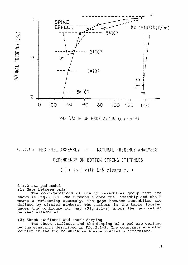
00

4 -,

CJ>2:LUC3

3 .

SPIKEEFFECT

0 20 40 60 80 100 120 140

RHS VALUE OF EXCITATION (cm • s~2)

Fig-3.1-7 PEC FUEL ASSEMBLY — NATURAL FREQENCY ANALYSISDEPENDENCY ON BOTTOM SPRING STIFFNESS

( to deal with E/N clearance )

3.1.2 PEC pad model(1) Gaps between pads

The configurations of the 19 assemblies group test areshown in Fig.3.1-8. The C means a core fuel assembly and the Rmeans a reflecting assembly. The gaps between assemblies aredefined by circled numbers. The numbers in the table locatedunder the configuration map (Fig.3.1-8) shows the gap valuesbetween assemblies.(2) Shock stiffness and shock damping

The shock stiffness and the damping of a pad are definedby the equations described in Fig.3.1-9. The constants are alsowritten in the figure which were experimentally determined.

71

C : Fuel AssemblyR : Reflecting Assembly

Exciting direction

AxialLevelcm255.8144.0

Gap 1

_-

Gap 2B1-A1cm0.1350.135

Gap 3Al-AOcm0.0450.045

Gap 4AO-A4cm0.0450.045

Gap 5A4-B7cm0.1350.135

Gap 6

—-

Fig."3.i.-8 Gaps in Group of 19 Fuel and Reflecting Assemblies72

[kg/mm 3AH

Ctests for the determinationof shroud stiffnessKg£ — F & AHwere measured H

1K2FC =

K2FCte

2K 2K

TT

Shock StiffnessShock DampingShock Duration0.55 /Steel-Steel Contact \

VCoefficient of Restitution/

Axial Level cm144255.85

K2F8600kgf/cm8850kgf/on

C4.774kgfs/cm4.912kgfs/cm

Fig.:3.i.-9 Determination of Shock Stiffness and Damping at Pads

3.1.3 PEC problems solved by the FINDS codeIn consideration to validate the FINDS model for the

colliding phenomena of assemblies, the largest test scale case(19 assemblies group and the most severe acceleration wave -TH.n.61) was selected in which collisions between pads areexpected to occur. The diagrid acceleration is plotted inFig.3.1-10. The one row assemblies shaded by inclined lines inFig.3.1-11 case is analyzed. The FINDS modeling is also shown inFig.3.1-11.

73

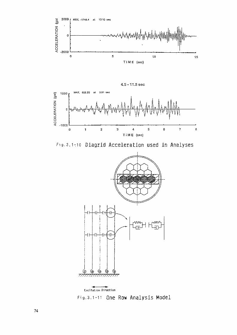
AC

CE

LER

ATI

ON

(g

al)

ACC

ELER

ATIO

N (

ga

l

-• ^

<?

çn

^C

O

0

\rt

\r

5"

^±

g

^

?,

$0

S T

^

23

«• ;>

n>

§' ^ \

t

(o^

1 JLY

Q\

'"T*-

^

/^ -L

\^

vT

y

i — t-

— (T)

/

33 Z3 CU h--

<< (/) H.

01 O a. ro

lu CO . I o O I-"

O> d n n m r—'

(D 03 CO ro CL zu 3=»

D3 tn ro co

m

M o O O

M O

.*• en m M ro o

S m

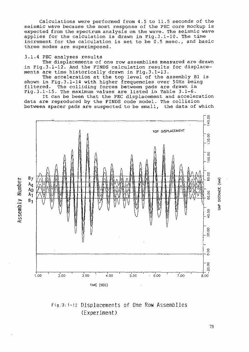
Calculations were performed from 4.5 to 11.5 seconds of theseismic wave because the most response of the PEC core mockup isexpected from the spectrum analysis on the wave. The seismic waveapplies for the calculation is drawn in Fig.3.1-10. The timeincrement for the calculation is set to be 0.5 msec., and basicthree modes are superimposed.3.1.4 PEC analyses results

The displacements of one row assemblies measured are drawnin Fig.3.1-12. And the FINDS calculation results for displace-ments are time historically drawn in Fig.3.1-13.

The acceleration at the top level of the assembly Bl isshown in Fig.3.1-14 with higher frequencies over 50Hz beingfiltered. The colliding forces between pads are drawn inFig.3.1-15. The maximum values are listed in Table 3.1-6.

It can be been that the PEC displacement and accelerationdata are reproduced by the FINDS code model. The collisionbetween spacer pads are suspected to be small, the data of which

QJ.0

£2

CDl/>to

«=C

1.00 2.00 3.00 4.00 5.00 6.00 7.00

TIME (SEC)

Fig.:3'. 1-.12 Displacements of One Row Assemblies(Experiment)

8.00

LJ0

StO

75

0\

MQJ B7

A4

AOA1

<UCOCO

<=C

DISPLACEMENT AT JOINT 1

1.00

Fig.3-.iris Displacements of One Row Assemblies(Analysis by FINDS Code: Reference Case)

2SLUO

ACCE

LERA

TIO

N (G

AL)

ACCE

LERA

TIO

N (G

AL)

ACCE

LERA

TIO

N (G

AL)

3=»

Z3 CD }-*

«< to h-» to

I -f^ 33 n n (T) h-• ro M co

er

o«<

^

-n

POf-H

(T

)Z

tO

CJ

T3CO

CD

O

Wo

n)o. (T

) 03 o T3 O LO W CD er

1600

0.

-120

00

-80

00

l l

l l

l

r-1m 'co m o

rt (D O N

-400

0.

0 40

00l

l l

l l

03

-160

00.

-120

00l

l l

-16

00

0 -1

2000

. -8

00

0l

l l

l l

-40

00

0

l l

l40

00

CD

» II

l M

ooo

lOlD

vj "o £C m "H MS

m

M }io u m O

IMPACT AT JOINT 5

Position

AQ-A4

A4-B?

100 200 i l

6 00 7 003 00 4 00 5 00

TIME (SEC)

Fig.î3;..rfï5 Shock Forces in One Array(Analysis by FINDS Code)

Table 3.1-6 FINDS Calculation Results of Reference case

a oo

zo

I

Max. Disp. mmMax. Acc.xlOESm-m/s2

Bl-56.5-1.533

Al51.45-1.729

AO50.99-1.222

A450.87-1.683

B758.231.587

Max . Force Upper PadMiddle Pad

B1-A1385.8-95.34

Al-AO314.8-70.52

AO-A4304.4-104.7

A4-B7412.1-94.03

were not measured in the experiments. From the design viewpoint, the shock forces at pads are required to be measured inthe core seismic experiments for the design use.

In the FINDS models both the secondary and the third modesdamping constants were set to be 3% from the consideration thatthe vibrational behaviors of this case are mainly controlled bythe first mode and that the low damping values may result inlarger displacements prediction. Then the FINDS overpredictsdisplacements a little. The experiments on the MONJU fuelassembly vibration characteristics showed more large damping as15% for the secondary mode. If large damping for higher modes areused, the consistency in displacements may proceeds. The dampingconstants for higher modes are also required to be measured.

78

Parameter surveys were performed to recognize the measuredcharacteristics. The survey cases are listed in Table 3.1-7where the damping factor is reduced along with inclusion of theadded mass effect. The three rows analysis was also performedthe model of which is drawn in Fig.3.1-16. The calculateddisplacements of the case D (low damping and added mass effectinclusion) and the case E ( three dimensional calculation)are drawn in Fig.3.1-17 and Fig.3.1-18, respectively.

From the information about the damping and the fluid masseffect, the case E the most appropriate for this test case. Fromthe three dimensional analysis, the response will be reduceda little compared with two dimensional analysis.

Table 3.1-7 Parameter Survey Cases for FINDS Analyses on PECexperiments

Case

ReferenceBCDEExperiment

Geometry

One RowOne RowOne RowOne RowThree Rows

Added Mass[Ma]

NoNoNoYesNoYes (Ref. (4) )

1st Mode Dam-ping %

54424l(Ref.(4))

Table 3.1-8 Comparison of Displacements

CaseReferenceBCDEExperiment

Bl56.554.342.751.853.148.0

Al51.547.437.746.246.9

AO51.047.337.345.247.551.0

A450.946.736.845.547.3

B758.253.643.351.953.650.0

79

Excitation Direction

F ig: 3; t-116 Three Rows Analysis Model

M.OJ

.C3S

"Z.

B?A4

AOA181

32

2.00 3.00 400 5.00 6.00 7.00 a oo

TIME (SEC)

i9- 3.-l~17 Displacements of One Row assemblies(Analysis by FINDS Code: Case D).

80

B?A„AOA1

TIU£ (SEC)

Fi g. 3 j1^,18 Displacements of Three Rows assemblies(Analysis by FINDS Code: Case E)

3.2 Analyses for RAPSODIE experiments3.2.1 RAPSODIE fuel assembly model

The overview of the RAPSODIE experiment is shown inFig.3.2-1.

Fuel assemblies and neutronic shield elements which wereused in the RAPSODIE core seismic tests are modeled by thedistributed mass and stiffness beams which are shown inFig.3.2-2.

Fig.3.2-1 Overview of RAPSODIE Test Apparatus

81

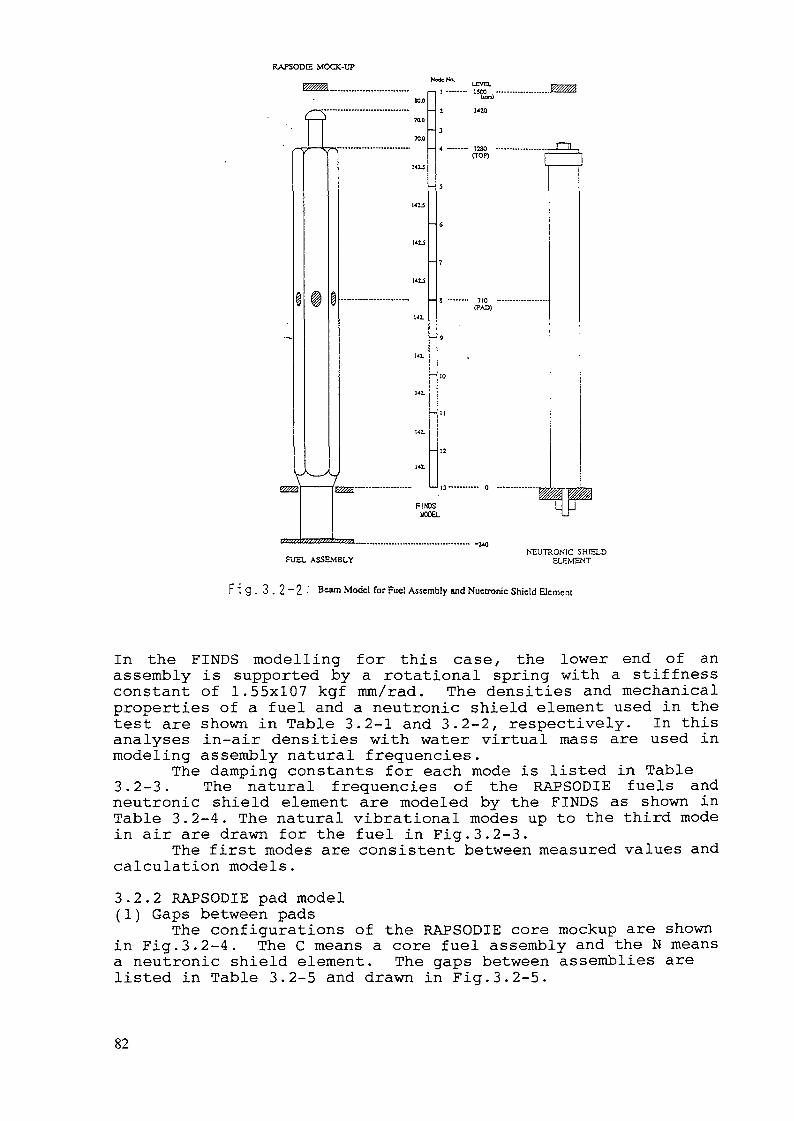
RAPSODE MOCK-UP

V

I2SOOOP)

710 •(PAD)

FINDSUOCEL

FUEL ASSEMBLYNEUTRONIC SHIELD

ELEMENT

F1 g . 3 . 2 ~ 2 •' Beam Model for Fuel Assembly and Nuecronic Shield Element

In the FINDS modelling for this case, the lower end of anassembly is supported by a rotational spring with a stiffnessconstant of 1.55x107 kgf mm/rad. The densities and mechanicalproperties of a fuel and a neutronic shield element used in thetest are shown in Table 3.2-1 and 3.2-2, respectively. In thisanalyses in-air densities with water virtual mass are used inmodeling assembly natural frequencies.

The damping constants for each mode is listed in Table3.2-3. The natural frequencies of the RAPSODIE fuels andneutronic shield element are modeled by the FINDS as shown inTable 3.2-4. The natural vibrational modes up to the third modein air are drawn for the fuel in Fig.3.2-3.

The first modes are consistent between measured values andcalculation models.3.2.2 RAPSODIE pad model(1) Gaps between pads

The configurations of the RAPSODIE core mockup are shownin Fig.3.2-4. The C means a core fuel assembly and the N meansa neutronic shield element. The gaps between assemblies arelisted in Table 3.2-5 and drawn in Fig.3.2-5.

82

Table 3.2-1 Mechanical Properties of; RAPSODIE Fuel 'Assemblies

El evat i on (m)TOP Bottom

-0.24

-0.06

0.0

0.088

0.12

1.2

1.252

1.28

1.42

-0.06

0.0

0.088

0.12

1.2

1.252

1.28

1.42

1.5

Densi ty103kg/m3

7.8

7.8

19.01

19.01

89.8

7.8

7.8

7.8

7.8

Cross Sec.Area(10~6m2)

251.

603.

953.

169.

169.

169.

953.

113.

1.

Young Modu.(101 'Pa)

1.9

1.9

1.9

1.9

1.9

1.9

1.9

1.9

1.9

Bend. Inert.(10-'2m4)

13069.

48254.

256340.

55957.

55957.

55957.

256540.

1018.

300000.

83

Tab le 372-2 ,Mechanical Proper t i es- o f - R A P S O D I E Neut ron ic iSKield Elements

E l evat ion (m)TOP Bottom

0.0

1.28

1.28

1.5

Densi ty103kg/m3

7.8

7.8

— —————————————

Cross Sec.Area(1(T6m2)

1810.

0.1

Young Modu.(10"Pa)

2.0

2.0

Bend. I n e r t .dcr'V)

260576.

300000.

T a b l e 3 .2 -3 Damp ing Constants o f R A P S O D I E Beam E lements

i n Ai r

Core Assemb ly

Neut ron ic S h i e l d

1st Mode

3 %

1 %

2nd Mode

3 %

1 %

3rd Mode

3 %

1 %

i n W a t e r

1st Mode 2nd Mode 3rd Mode

Core Assembly 5 % 5 %

Neut ron i c S h i e l d 3 %

84

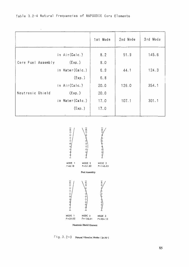
Table 3.2-4 Natural Frequencies of RAPSODIE Core Elements

i n Ai r (Cale. )Core F u e l Assembly (Exp.)

i n Water(Calc. )(Exp.)

i n Ai r(Calc. )Neut ron ic S h i e l d (Exp. )

in Water(Calc. )(Exp.)

1st Mode

8.28.06.96.820.020.017.017.0

2nd Mode

51.9

44.1

126.0

107.1

3rd Mode

145.6

124.3

354.1

301.1

MODE 1 MODE 2 MODE 3F=8.19 F=51.8S F=145.63

Fuel Assembly

MODE 1 MODE 2 MODE 3F=20.02 F= 126.01 F=354.13

Neutronic Shield Element

F i g . 3. 2-3 Natural Vibration Modes (in Air)

85

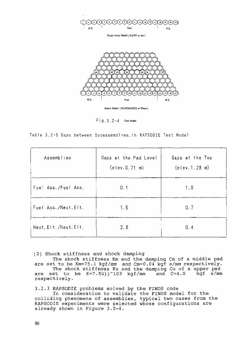
Single Array Mcxiel ( RAP87 in Air )

jk70CjCjC?T?°JLJ^^tJLj^^^*)CjCjO • ji.

00000000000000N.S. • Fuel N S.

Matrix Model ( RAPZIMME32 in Water )

F 1 9 . 3 . 2 - 4 Corc Modd

Table 3.2-5 Gaps between Subassemblies,i n RAPSODIE Test Model

Assembl i es Gaps at the Pad Level(elev.0.71 m)

Gaps at the Top(elev.1.28 m)

F u e l Ass./Fuel Ass. 0.1 1.0

Fuel Ass./Neut.Elt, 1.5 0.7

Neut. Elt./Neut. E l t . 2.8 0.4

(2) Shock stiffness and shock dampingThe shock stiffness Km and the damping Cm of a middle pad

are set to be Km=75.1 kgf/mm and Cm=0.04 kgf s/mm respectively.The shock stiffness Ku and the damping Cu of a upper pad

are set to be K=7.5u»~103 kgf/mm and C=4.0 kgf s/mmrespectively.3.2.3 RAPSODIE problems solved by the FINDS code

In consideration to validate the FINDS model for thecolliding phenomena of assemblies, typical two cases from theRAPSODIE experiments were selected whose configurations arealready shown in Figure 3.2-4.

86

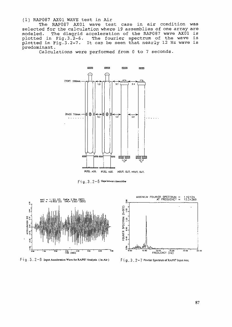
(1) RAP087 AX01 WAVE test in AirThe RAP087 AX01 wave test case in air condition was

selected for the calculation where 19 assemblies of one array aremodeled. The diagrid acceleration of the RAP087 wave AX01 isplotted in Fig. 3.2-6. The fourier spectrum of the wave isplotted in Fig.3.2-7. It can be seen that nearly 12 Hz wave ispredominant.

Calculations were performed from 0 to 7 seconds.

(TOP) 1280mm—--

§

v33 :

L

ö

^^

1.0

}++(0.1

1 \

1

} %

CO.A

»-^

/V2J& WA

7777B

fl —— 1

V

] C 0 4 J [

-< ——— >2.8

b i

T — I

!|Jr

}

%FUEL ASS. FUEL ASS. NEUT. ELT. NEUT. ELT.

Fig 3 2~5

MAX - 1.123 (Cl TIME- 239« (SEC)WIN - -09S2 (G) TIME- 2.021 (SEC)

a on l OO Ï 00 i 00 4 OO 1.OO 4.00 7 OOTIME (SEC)

F 1 g . 3 . 2 - 6 Input Acceleration Wave forRAPS? Analysis ( in Air)

3s

MAXIMUM FOURIER SPECTRUM = 1 42124AT FREQUENCY = 12.24369

10 00 70 00 iO 00FREQUENCY (HZ)

F i g . 3 . 2 - 7 Fourier Spectrum of RAP87 Input Ace.

87

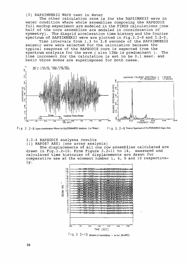
(2) RAPZIMMER32 WAVE test in WaterThe other calculation case is for the RAPZIMME32 wave in

water condition where whole assemblies composing the RAPSODIEfull mockup experiment are modeled in the FINDS calculations (onehalf of the core assemblies are modeled in consideration ofsymmetry) . The diagrid acceleration time history and the fourierspectrum of RAPZIMMER32 wave are plotted in Fig. 3. 2-8 and 3.2-9.

Time intervals from 1.3 to 3.8 seconds of the RAPZIMMER32seismic wave were selected for the calculation because thetypical response of the RAPSODIE core is expected from thespectrum analysis for the wave ( also 12Hz is predominant ) . Thetime increment for the calculation is set to be 0.1 msec, andbasic three modes are superimposed for both cases.

MAX - 1 533MIN - -1 272

(C) TIME- 3 550 (SEC)(0) TIME- 3 ISO (SEC)

I

MAXIMUM FOURIER SPECTRUM = 1 66335AT FREQUENCE = 1240234.

œbjc:

TIME (SEC)10 00 20 00 JO OO

FREQUENCY (HZ)

3 2-8 lnpu t Acceleraüon Wave for RAP23MME32 Analysis < in Water ) Fig 3 . 2 - 9 F°uncr Spectrum of RAP22MME32 Input Ace.

3.2.4 RAPSODIE analyses results(1) RAP087 AX01 (one array analysis)

The displacements of all one row assemblies calculated aredrawn in Fig.3.2-10. From Figure 3.2-11 to 14, measured andcalculated time histories of displacements are drawn forcomparative use at the element number 1, 4, 5 and 10 respective-

191817161514

' 13O 12^ 112 10

m 87654321

.Itkln-H»«!!......... .. •WW wtftw^

Mi&^^^Billf-KMIKEM^^iSltî^lSi,,

\lttp VrtW^^^x-V^VN^MViW ^fVVAVS'*W>Wfr^'^W*#r)ljHNtiMrtNHWi>l'M#*t*t*

TIME (SEC)

F1 g . 3 2-10 Motion of Assemblies - m Air (RAP87)

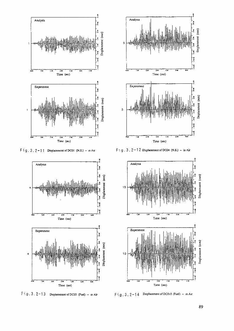
Analysis

...... AJÉIll

c t o ö t o o

-T Q

iOO 440 3.00 «00

Time (sec)

F i g . 3 . 2 - 1 1 Displacement of DC01 (N.S.) -- m Air

Time (see)

Fi g . 3 . 2-1 2 Displacement of DC04 (N.S.) - in Air

< oo I.OO ZJM iOO «00 S.OO

Time (sec)

10

Experiment

I.OO ioo 4 00 XOO

Time (sec)

F 1 g . 3 . 2 - 1 3 Displacement of DCOS (Fuel) -in Air F1 g . 3 . 2 - 1 4 Displacement of DC010 (Fuel) - m Air

89

In fig. 3. 2-15, the maximum displacement values arecompared for all elements . The consistency is thought to befairly well .

The calculated shock forces at spacer pads are shown inFig. 3. 2-16.

O Experiment• FINDS

20

10-

QHl'i -10s

-20

1.0

U.G 0.5-

0.01 Z 3 4 S 6 7 8 9 1011 1 2 1 3 1 4 1 5 161718 19

Fuel No.

f W y ¥—:—i—l—i—i—i—:—i—:—t—!—t * ^ ~1 2 3 4 5 6 7 8 9 1 0 1 1 1 2 1 3 1 4 1 5 1 6 1 7 1 8 1 9 2 0

F 1 g . 3 . 2 - 1 5 Maximum Displacements - in Air (RAP87)

Gap Number

F 1 g . 3 . 2 - 1 6 Maximum Impact Forces at Pad Elevation - in Air (RAP87)

(2) RAPZIMMER32 (three dimensional analysis)In fig.3,2-17, all motions of the full mock-up test

(RAPZIMMER32) are plotted.From Figure 3.2-18 to 31, measured and calculated time

histories of each assembly displacement are drawn for comparativeuse at the element number 1, 4, 5, 10, 15. 16, 19, 86, 89, 90,92, 95, 96 and 99 respectively. In Fig.3.2-32, calculatedmaximum displacements of central array are compared with measureddata. Souor Elevation

F i g . 3 . 2-17 Motion of Mock-up Assemblies - in Water (RAPZIMME32)

90

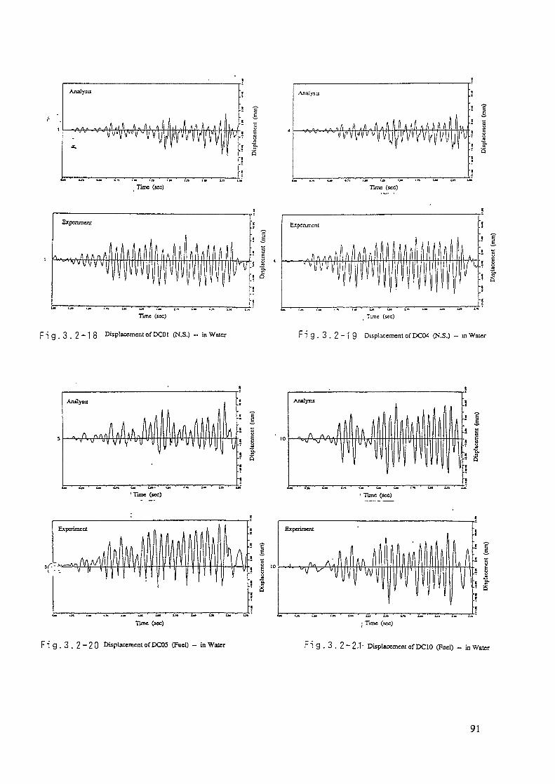
Time (we) Tone (sec)

Time (sec)

F i g . 3 . 2-18 Displacement of DCOI (M.S.) -- in Water

Time (sec)

F ig. 3. 2-19 Displacement of DC04 (N.S.) - in Water

Tune («ec) • Time (sec)

"nine <iec]

F i g . 3 . 2 ~ 2 0 Displacement of DC05 (Fuel) - in Water

; Time (sec)

Fi g . 3 . 2 -2-1- Displacement of DC 10 (Fuel) - in Water

91

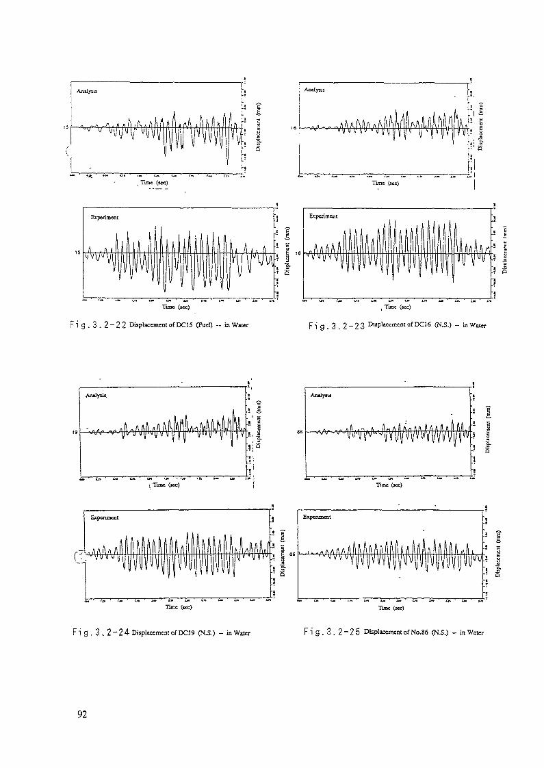
Time (tec)

Fi g . 3 . 2 -22 Displacement of DCI5 (Fuel) - in Water

, Tim: (sec)

F i g . 3 2-23 ^PkccmentofDCie (N.S.) -- in Water

Tune (tec) Tune (sec)

Fi g . 3 . 2-24 Displacement of DC19 (N.S.) - in Water F i g . 3 . 2 - 2 5 Displacement of No.86 (M.S.) - in Water

92

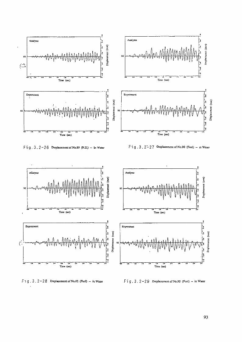
Analysa.

Tune (sec)

•5.' S

Time (sec)

Tune (tec) Time (sec)

F i g . 3. 2-26 Déplacement of No.89 (N.S.) - in Water F i g . 3 . 2 ~ 2 7 Displacement of No.90 (Fuel) - in Water

Time (sec) Time (sec)

Time (sec) Time (jcc)

F 1 g . 3 . 2 - 2 8 Displacement of No.92 (Fuel) - in Water F i g . 3 . 2-29 Displacement of No.95 (Fuel) - in Water

93

A/Wtf

Time (sec)

p.

Analym

Tune

Tune («cc) Time (tec)

F ig. 3. 2 ~ 3 0 Displacement of No.% (N.S.) - in Water F l g . 3 . 2 - 3 1 Displacement of No.99 (N.S.) - in Water

° Experiment• FINDS

20

ID-

0-

O O». *

* O

0 8 . 0 . 5

1 2 3 4 S 6 7 3 9 1011 1213141516171819

Fuel No.

l g . 3 . 2 — 3 2 Maximum Displacements of Central Array

'- in Water (RAPZIMME32)

From these data, it can be seen that the maximum values areconsistent with each other although the calculated displacementsof neutronic shield elements are smaller than measured valuesin time historical domain. In addition it may exist some timelag in measured data against the absolute time history becauseif we slide calculated displacements in time axis, we can getgood agreement between calculations and measured displacementhistories.

94

The core-wide distribution of maximum displacements valuesof all elements are written in Fig.3.2-33 and the core-widemotion of the mock-up test elements of the RAPZIMMER32 are shownin Fig.3.2-34.

We can see that core fuels mainly response to the seismicwave and they are restricted by the neutronic shield elements.Also by the three dimensional comparison, it can be said thatthere exists consistency between the measurements and thecalculation. Some discrepancy existing during the time 35 to 40seconds may due to measured data reprocessing error.

The maximum impact forces at the pad elevation are drawnin fig.3.2-35.

In the FINDS the neutron displacements are underpredictedfor both one row and three dimensional case against measuredvalues. The cause of this discrepancy cannot be revealed by thelack of fine experimental data now. If possible the measureddata should be studied more carefully for natural frequency anddamping etc.

Through the three dimensional analyses for the PEC and theRAPSODIE cores, it can be concluded that if we use the threedimensional analysis we can get slightly lower response both inthe displacements and the shock forces by the dispersion effectsin the crossing directions.

or FUCL ... X-OIRCCTION <wo TIMCI

an to NO. - i JOIKT NQ. - l

4.O 4.4 «.1 -3.7 -3. » -3.3 4,4 4.3 4.3 4.4,

-3.O -4.0 -4. T -4.» 1.2 8.4 7.4 -O.I -«.3 -«.3 4.4 4,4 4.2 4. T

-3.3 -3.2 -3.3 -3.3 *.4 *.3 8.» -«.3 -».3 -IO.O -».3 4.T 4.8 4.7 3.3

-3.4 -3.3 -3.8 -4.0 8.3 IO. l 1O. l T.O -T.3 -1O.* -1O.8 -*.4 -3.2 3.3 3.3 3.4

.3 -*, I -3.7 -3.» *.4 *.* 1O.7 1O.4 -T.4 -IO.7 -II.3 -11.3 -11.3 -4.1 3.3 3.3 3.8

-«.8 -*.3 3.4 T.fl 1O.4 1Û.4 11.3 1O.2 -11.0 -11.4 -12.2 -Ll . l -11.3 3.4 3.t fc.A 4.3

.* -*-4 -3.T IO.? 12.0 10.* 11.7 11.3 —IO.* -11.3 —12.2 —12.4 —11.3 — I I , 4 4.2 4,2 fc.T 4,

MAX, VALUE Or AU. ... AT FUG. NO. 13

OlSPlACa-CNT OF FUG. ... Y-DIRCCTtON CAHD TtnCÏ

(MIO NO. • 1 JOCKT MO. - 1

1.7 2.3 2.3 2.4 2.3 2.2 2.1 2.O 1.T 2.O l .Q 1.4 1.»

1.3 1,3 1.3 1.7 —4,0 -3.1 -2.4 -2.4 -3.2 -3.V l.O 1.3 1.3 1.2

1.3 t.l -1.2 1.4 -3.3 -3.t -3.1 -2.2 -2.4 -2.» -3.T -3.7 t.3 -l. l -1.2 1.3

O.O 0.0 O. O O. O O.O O.O 0.0 O. O O.O O.O O.O 0.0 O.O O.O O.O O.O O.O O. O O.O

n**. VAUX or AU. ... AT rue. NO. ai

F i g . 3 . 2 ~ 3 3 Core-wide Distribution of Maximum Displacement - in Water (RAPZIMME32)

95

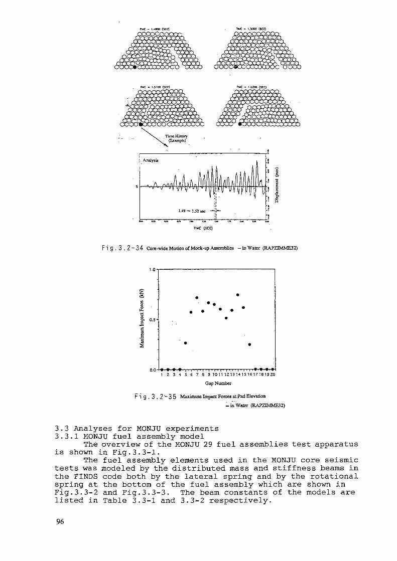
i.sooo (sec)

nue - 1.5100 <secî

TIME (SEC)

F i g . 3 . 2 ~ 3 4 Core-wide Motion of Mock-up Assemblies -in Water (RAPZIMME32)

1.0'

§Ê

3

0.5

1 2 3 4 5 6 7 8 91011121314151617181920

Gap Number

F i g . 3 . 2 - 3 5 Maximum Impact Forces at Pad Elevation- in Water (RAP23MME32)

3.3 Analyses for MONJU experiments3.3.1 MONJU fuel assembly model

The overview of the MONJU 29 fuel assemblies test apparatusis shown in Fig.3.3-1.

The fuel assembly elements used in the MONJU core seismictests was modeled by the distributed mass and stiffness beams inthe FINDS code both by the lateral spring and by the rotationalspring at the bottom of the fuel assembly which are shown inFig.3.3-2 and Fig.3.3-3. The beam constants of the models arelisted in Table 3.3-1 and 3.3-2 respectively.

96

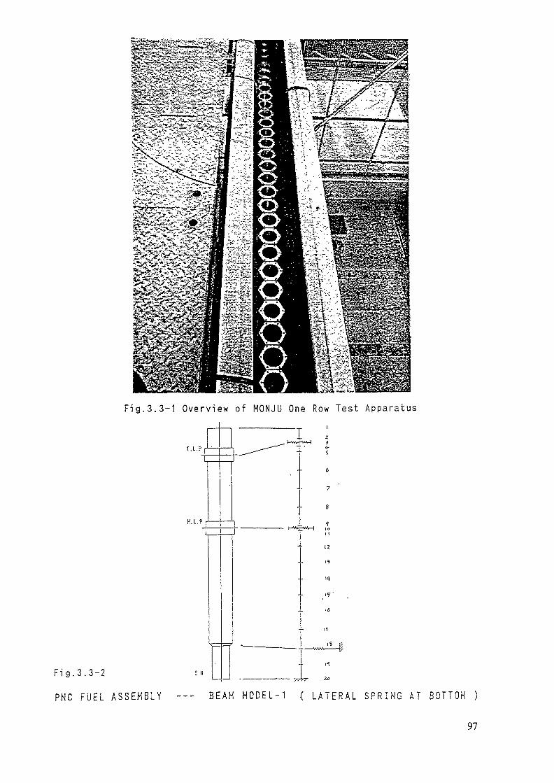
Fig.3.3-1 Overview of MONJL) One Row Test Apparatus

T.L.PI

X.LP

Fig.3.3-2

PNC FUEL ASSEMBLY

E II

B E A M M O D E L - 1 ( L A T E R A L S P R I N G A T B O T T O M )

97

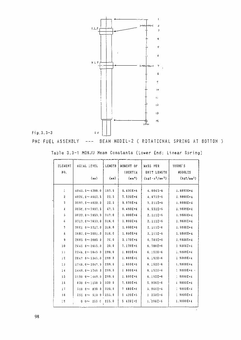
T.L.P

H L P

Fig.3.3-3

P N C F U E L A S S E M B L Y

E X

1 1

12

13

~X

B E A H M O D E L - 2 ( R O T A T I O N A L S P R I N G A T B O T T O M )

Tab le 3 .3-1 MONJU Meam Constants ( L o w e r End: L inear S p r i n g !

E L E M E N TN O .

1

2

3

4

5

$

7

8

9

10

1 1

12

13

H

15

16

17

18

19

A X Ï A L L E V E L

( m o )

4 0 4 2 . 5 ~ 4 2 0 0 . 0

4 0 2 0 . 0~ 4 0 4 2 . S

3 9 9 7 . 5 ~ 4 0 2 0 . 0

3 9 5 0 . 0 — 3 9 9 7 . 5

3 6 3 3 . 0~ 3 9 5 0 . 0

3 3 1 7 . 0 - 3 6 3 3 . 0

3001 0 -3317 .0

2 6 8 5 . 0 -3001 .0

2 6 6 5 0 - 2 6 8 5 0

2 6 4 5 0 — 2 6 6 5 . 0

2 3 4 6 . 0 — 2 6 4 5 0

2 0 4 7 0 — 2 3 4 6 . 0

1 7 4 8 . 0 — 2 0 4 7 . 0

1 4 4 9 . 0- 1 7 4 8 0

1 1 5 0 0- 1 4 4 9 . 0

830 0—1 150 0

510 0— 830 0

255 0— 510 0

0 0- 255 C

L E N G T H

(BO)

157. 5

22. 5

22. 5

4 7 . 5

317. 0

316. 0

316. 0

316. 0

2Û. 0

20. 0

2 9 9 . 0

299 0

2 9 9 . 0

2 9 9 . 0

2 9 9 . 0

320 0

3 2 0 . 0

255. 0

2 5 5 . 0

MOHEKT OF

I N E R T I A(an 4 )

6. 4 3 0 E + 6

7. 9 2 0 E + 6

9. 9 7 0 E + 6

8. 4 8 0 E + 6

1. 800E + 6

1. 8 0 0 E + 6

1. 8 0 0 E + 6

1. 8 0 0 E + 6

3. 1 7 0 E + 6

3. 170E + 6

1. 8 0 0 E + 6

1. 8 0 0 E + 6

1. 8 0 0 E + 6

1 8 0 0 E + 6

1. 8 0 0 E + 6

7. 6 8 0 E + 6

1 6 8 0 E + 6

5 4 2 0 E + 5

5 4 2 0 E + S

MASS PER

U N I T L E N G T H

( X g f - s V n n 2 )

4. 004E-6

4. 671E-6

7. 211E-6

6. 531E-6

2. 111E-6

2. 111E-6

2. 111E-6

2. i l lE-6

6. 7 8 6 E - 6

6. 7 8 6 E - 6

6. 1 S 2 E - 6

6. 152E-6

6. 1 5 2 E - 6

6. 1 S 2 E - 5

6. 1 5 2 E - 6

5. 3 0 6 E - 6

S. 9 0 6 E - 6

1 208E-6

1 /208E-6

Y O U H G ' S

M O D U L E S

{ k g f / n m 2 )

1 .9800E+4

1. 9800EH

1.9800Et4

1.9800E-M

1 . 9 8 0 0 E + 4

1 . 9 8 0 Q E + 4

1 . 9 8 0 0 E + 4

1 . 9 8 0 0 E + 4

1 . 9 8 0 0 E + 4

1 9 8 0 0 E + 4

1. 9 8 0 0 E + 4

1 9 8 0 0 E + 4

1. 9 8 0 0 E + 4

1 9 8 0 0 E + 4 -

1 9 8 0 0 E + 4

1 9 8 0 0 E + 4

1 9 8 0 0 E + 4

1 9 8 0 0 E + 4

1. 9 8 0 0 E + 4

98

Table 3.3-2 MONJU Meam Constants (Lower End: Rotational Spring)

E L E M E N T

NO.

1

2

3

4

5

6

7

8

9

10

il

12

13

A X I A L L E V E L

( m m )

4 0 2 0 . 0 - 4 2 0 0 . 0

3 9 5 0 . 5 — 4 0 2 0 . 0

3 6 3 3 . 0 - 3 9 5 0 . 0

3 3 1 7 . 0 - 3 6 3 3 . 0

3001 . 0 — 3 3 1 7 . 0

2 6 6 5 . 0— 3001 . 0

2 3 4 6 . 0 - 2 6 6 5 . 0

2 0 4 7 . 0 - 2 3 4 6 . 0

1 7 4 8 . 0 - 2 0 4 7 . 0

1 4 4 9 . 0— 1748 . 0

1150. 0 - 1 4 4 9 . 0

8 3 0 . 0 - 1 1 5 0 . 0

5 1 0 . 0 — 8 3 0 . 0

L E N G T H

( a m )

180. 0

70. 0

3 1 7 . 0

316. 0

316. 0

316. 0

3 3 6 . 0

319. 0

2 9 9 . 0

2 9 9 . 0

2 9 9 . 0

3 2 0 . 0

320. 0

M O M E N T OF

I N E R T I A

( m i 4 )

S. 4 3 0 E + 6

8. 4 8 0 E - I - 6

1. S O O E - i - 6

1. 8 0 0 E + S

1. 8 0 0 E + 6

1. 8 0 Û E + 5

1. 8 0 0 E + 6

1. 800E + S

1. 8 0 0 E + 6

1. 8 Û O E + 6

1. S O O E - f - 6

7 . 6 8 0 E + 6

7. 6 8 0 E + 6

M A S S P E R

U N I T L E N G T H

( k g f - s V m m 2 )

3. 5 0 3 E - 6

6. 2 0 4 E - 6

2. 111E-6

2. 111E-6

2. 111E-6

1. 985E-6

5. 7 6 6 E - 6

6. 152E-6

6. 152E-6

6. 1 5 2 E - 6

6. 152E-6

5 . 9 0 6 E - 6

5 . 9 0 6 E - 6

YOUN<T S

M O D U L E S

( k g f / m n 2 )

1. 9 8 0 0 E + 4

1. 9 8 0 0 E + 4

1. 9800E-M

1. 9 8 0 0 E + 4

1. 9 8 0 0 E + 4

1. 9 8 0 0 E - M

1. 9 8 0 C E + 4

1. 9800E+4

1. 9 8 0 0 E + 4

1. 9 8 0 0 E + 4

1. 9 8 0 0 E + 4

1. 9 8 0 0 E + 4

1. 9 8 0 0 E - M

A rotational spring with a stiffness constant of 1.55x107kgf mm/rad is attached at the lower end. The natural frequenciesand modes in air of the MONJU fuel are shown in Fig.3.3-4. Thefirst frequencies of the both models are consistent with themeasured data. The higher modes frequencies cannot be checked bythe lack of the measured data.3.3.2 MONJU pad model(1) Gaps between pads

The configurations of the core are shown in Fig. 3. 3-5. Thegaps between assemblies are 0.7 mm at upper pads level and 1.0mm at the middle pads level.(2) Shock stiffness and shock damping

The shock stiffness Km and the damping Cm of a middle padare set to be Km=4400 kgf/mm and Cm=0.375 kgf s/mm respectively.

The shock stiffness Ku and the damping Cu of a upper padare set to be K=140000 kgf/mm and C=2.42 kgf s/mm respectively.3.3.3 MONJU problems solved by computer codes

In order to validate the core seismic analysis models,typical two cases from the MONJU experiments were selected. Oneis the pads collision tests and the other one is the 29 assem-blies array experiment.

99

FBR PNC MONJU-TYPE FUEL IN flIR tKX=8.0E02)NflTURflL VIBRRTION MODES

FBR PNC MONJU-TYPE FUEL IN RIR (KR=4.3E07)NflTURRL YIBRflTION MODES

MODE 1 MODE 2 MODE 33.51 CHZ) 16.86 (HZ) 52.02 (HZ!

MODE 1 MODE 2 MODE 33.50 (HH) 18.00 (HZ) 58.00 (HZ)

MODEL-1( LATERAL SPRING AT BOTTOM )

MODEL-2( ROTATIONAL SPRING AT BOTTOM )

• F i g . 3 . 3 - 4 PNC FUEL ASSEMBLY .— NATURAL FREQUENCY ANALYSIS

One Row Test

Cluster Test

Fig.3.3-5 MONJU Core Map and Test Sections

100

(1) Pads collision test analysisThe upper and middle pads collision test results were

analyzed by the FINDS code. The configuration of the experimentsis drawn in Fig. 3.3-6.

Initialdisplacement

1 Test subassembly2 Support3 Weight4 Load cell5 Wire6 Tenion releae equipment7 Tension equipment

^^^^^^^^^

Fig.3.3-6 MONJU Collision Test Apparatus

(2) One array of 29 assemblies vibration test in waterThe other calculation case is the 29 assemblies vibration

test in one array shaken within water.The analysis was performed by the multi-purpose structural

analysis code ANSYS which uses the direct integration and theGuyan reduction methodology.

The diagrid acceleration time history and the fourierspectrum of the hypothetically largest earthquake wave S2 whichis set for the design use are plotted in Fig.3.3-7 and 3.3-8.

Times from 7 to 13 seconds of the wave were selected forthe calculation because the typical response of the MONJU coreis expected from the spectrum analysis for the wave ( 12 Hz ispredominant ) . The time increment for the calculation is set tobe 0.05 msec.

101

Analysis Interval : 7~13Sec.

I * ' I I I

T i me (Sec.)

Fig.3.3-7 Acceleration History for Monju Verification Analysis

WcCDO

OCDQ.

CO

CD

OCL-

100

00

ao

70

60

so

20

10

.0 1.7 5.11 S.I 0.0 0.5 10.2 11.B lï.S 15.3 17.0

Frequency (Hz)Fig. 3. 3-8 Power Spectrum of Acceleration History

for Monju Verification Analysis

3.3.4 MONJU analyses results(1) Pads collision tests

The impact force at the upper pad is drawn in Fig. 3. 3-9 andFig.3.3-10 for taking into calculation of second modes and thirdmodes respectively.

The impact force at the middle pad is drawn in Fig.3.3-11and Fig.3.3-12 for taking into calculation of second modes andthird modes respectively.

Comparison with the measured data shows that the impactforces can be analyzed well by taking into account three modesfor middle pads both in the value and in the shape. The upper padimpact force value is overpredicted which may means that theupper pad impact phenomena cannot be modeled by the normal beamstiffness.

103

IMPACT FORCE (TON)

20

HU. taxa, cxt» ISTÎJ.»TIHC <8KÏ 0.0731

o.oa a.ai 0.02 0.03 o.o< a.os a.as 0.07 0.05 o.og o.io

COLLISION AT TOP PAD •-• considering -2nd modeFi g.3.3-9 PNC FUEL ASSEMBLY —— COLLISION TEST ANALYSIS

IMPACT FORCE (TON)

20

MX. raœc. tKoi unc.tTIKC (8CCÏ 0.0731

O.OQ 0.01 0.02 0.03 0.04 O.OG 0.06 0.07 0.09 0.00 0.10

TIME (SEC)

COLLISION AT TOP PAD -•• considering —3rd mode

Fi g.3.3-10 PNC FUEL ASSEMBLY —— COLLISION TEST ANALYSIS

104

IMPACT FORCE (TON)

rax. rose t PC»)

n« utc)

IHPRCTC3.QOTOH)

0-00 0.01 0-02 0.03 C.Q* 0-05 0.08 0-07 0.08 0.00 0.10

COLLISION AT MIDDLE PAD ••• considering -2nd node

F i g . 3 . 3 - 1 1 PNC FUEL ASSEMBLY —— COLLISION TEST ANALYSIS

IMPACT FORCE (TON)

3

2 •

MAX. fORCE (KG) 1449.5

TIME (SEC) O.OT43

D I S P L A C E M E N T

0.00 0.05

TIME (SEC)

0.10

COLLISION AT M I D D L E PAD • • • considering ~ 3rd mode

Fig.3.3-i2pNC FUEL ASSEMBLY — COLLISION TEST ANALYSIS105

(2) One row 29 assemblies analysesIn fig.3.3-13, all assemblies motions of the one row

assemblies are plotted at upper pad and middle pad levels.The side views of the 29 assemblies vibrations are plottedin Fig.3.3-14 for the time duration from 11 sec. to 11.2 sec.with time step of 0.02 sec. where the most responses occur. Therow consists of three types assemblies (core fuels, blanket fuelsand shield elements), some incoherences can be seen. The impactat pads are explained by the time lag in displacements betweenelements in the core center region. The impacts at the peripheralregion are off course explained by the response differencesbetween core elements and the barrel.

In Fig.3.3-15 displacements of the outer most element andthe 6th element from the peripheral (blanket fuel) are comparedwith measured data.

Q 1 0 . 0 -

5. 0-ar

o. o- .7. 0 1. 5 8. 0 9. 5 1 0. 0 1 0. 5 1 1. 0

T i m e ( s e c . )U p p e r P a d

7. 0 7. 5 9. 5

T i m e ( s e c . )M i d d l e P a d

1 0. 0 1 0. 5 1 1. 0

F i g . 3 . 3 - 1 3 P a d s L e v e l s D i s p l a c e m e n t s o f M O N J U A s s e m b l i e s

106

£01

- 9 9 -y

coco

COd.

CDCO CO

CO

coco

CO

CO

rooco

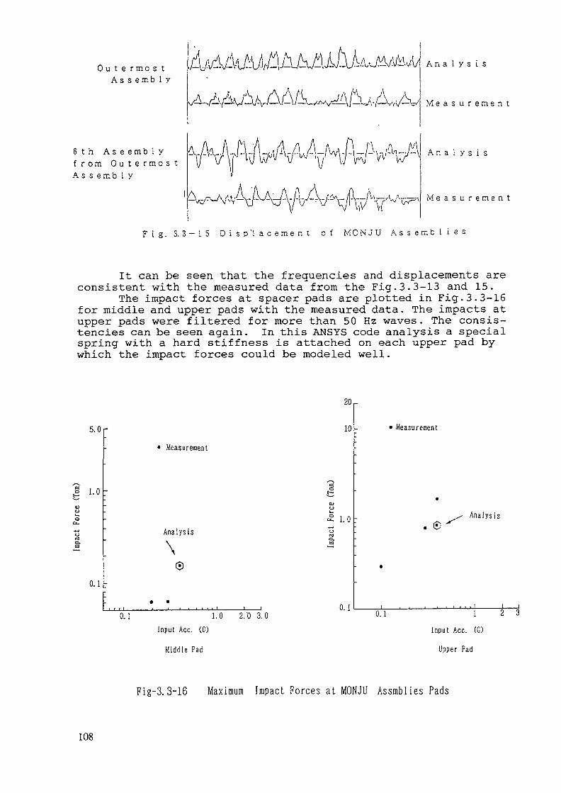
Impa

ct Fo

rce

(Ton

)o oo

01 o

OQ GO

CO i 05

CO X •o CO o O OJ o ci;

in 3 er -a CO O-

r° 0

Impa

ct Fo

rce

(Ton

)

\

en et

C HI

(DW

O

H-

H d

>tJ

HO

H

- O

(D

tr 3

H- H

" (D en

D)

3 h"

rt (DCO

(D

H- £

T3 »8

0»

o

$; »SsT

w ®

H, o t-i cn

n (t)

H- (

Dcn

HI (.

..H

i 3

03

.O

(Dfi

U

M W

H(X

3

*

t; S S' S

o o cn H- co (D r

trt

nh"

D

)g

<|

y'T

) H

-D)

et

GO tr

(D

rt H> Î3

- (D

SœS

P.

*~

COH

i <*

O *R

isH

- W o

3 O r

ta

o»(ü

O

1_) (

rfw

CD

CD S

PJ Ô

.

08 a m

(D &> n

S

<D (D

<s < ?

0)

O H

- f1

rtiQ

rt •

p-ffi

w

t^'

i .

cn

•Ö c

nTD

p-

(D cn

12 0*2

co t-3 il H

.(D

g"O

pu

o n

P

etcn

encn

euI

rt

OJ I

O (D 3 (D et co D) h CD

• oq os co I Ul o •a t» o a> 3 CD D o c; 3 cr CD M

CD PJ CD 3

*J>

»-h

Oî

W

M

rt

(a

O

p-Ct

. 3

3

>O

" O

M

^

C

CD

CD

3

•t cr

3 —

o

xM

O C>

rt

M

COM

-1CD

g

3 5

ç. >> r t> s CD (U CO •t CD 3 CD

P t» X M

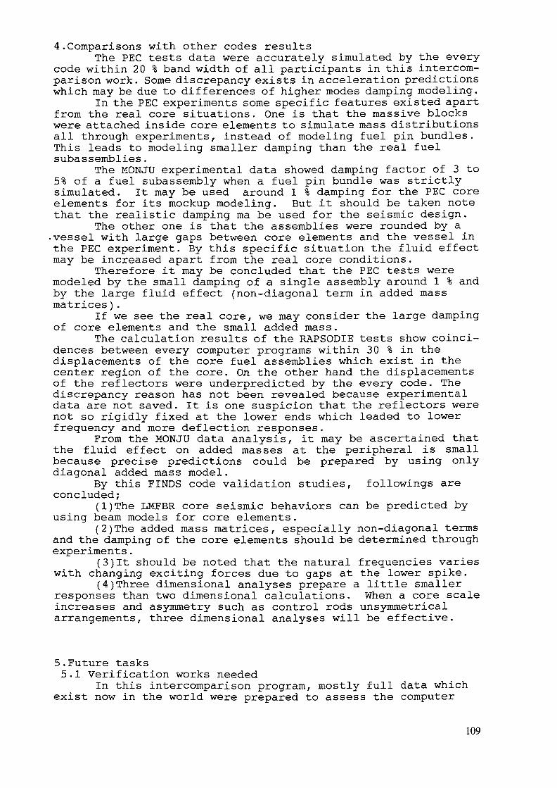
4.Comparisons with other codes resultsThe PEC tests data were accurately simulated by the every

code within 20 % band width of all participants in this intercom-parison work. Some discrepancy exists in acceleration predictionswhich may be due to differences of higher modes damping modeling.

In the PEC experiments some specific features existed apartfrom the real core situations. One is that the massive blockswere attached inside core elements to simulate mass distributionsall through experiments, instead of modeling fuel pin bundles.This leads to modeling smaller damping than the real fuelsubassemblies.

The MONJU experimental data showed damping factor of 3 to5% of a fuel subassembly when a fuel pin bundle was strictlysimulated. It may be used around 1 % damping for the PEC coreelements for its mockup modeling. But it should be taken notethat the realistic damping ma be used for the seismic design.

The other one is that the assemblies were rounded by a•vessel with large gaps between core elements and the vessel inthe PEC experiment. By this specific situation the fluid effectmay be increased apart from the real core conditions.

Therefore it may be concluded that the PEC tests weremodeled by the small damping of a single assembly around 1 % andby the large fluid effect (non-diagonal term in added massmatrices).

If we see the real core, we may consider the large dampingof core elements and the small added mass.

The calculation results of the RAPSODIE tests show coinci-dences between every computer programs within 30 % in thedisplacements of the core fuel assemblies which exist in thecenter region of the core. On the other hand the displacementsof the reflectors were underpredicted by the every code. Thediscrepancy reason has not been revealed because experimentaldata are not saved. It is one suspicion that the reflectors werenot so rigidly fixed at the lower ends which leaded to lowerfrequency and more deflection responses.

From the MONJU data analysis, it may be ascertained thatthe fluid effect on added masses at the peripheral is smallbecause precise predictions could be prepared by using onlydiagonal added mass model.

By this FINDS code validation studies, followings areconcluded;

(1)The LMFBR core seismic behaviors can be predicted byusing beam models for core elements.

(2)The added mass matrices, especially non-diagonal termsand the damping of the core elements should be determined throughexperiments.

(3)It should be noted that the natural frequencies varieswith changing exciting forces due to gaps at the lower spike.

(4)Three dimensional analyses prepare a little smallerresponses than two dimensional calculations. When a core scaleincreases and asymmetry such as control rods unsymmetricalarrangements, three dimensional analyses will be effective.

5.Future tasks5.1 Verification works needed

In this intercomparison program, mostly full data whichexist now in the world were prepared to assess the computer

109

models for core seismic analyses. But the lack of the spacer-padsimpact measurements except the MONJU core peripheral region data,it is uncompleted to validate the shock force modeling. Measurem-ents of impact forces at spacer-pads are expected in the innercore regions.

In addition, the effect of the sodium free surface onresponse behaviors is valuable point to be studied. And the fluid-structure interaction effect by the fluid between core elementsand the vessel should be also experimentally clarified by usingactual core geometry mockups.

The damping characteristics should be also defined throughexperiments and theoretical fields.

The interactive movements both horizontal and verticaldirections are important area to be resolved in future, becausethe seismic waves contain both directions accelerations. Theexperiments by using a shaking table will be fruitful. Theshaking table should have capability to vibrate horizontally andvertically at the same time. A computer program to treat axialvibration behaviors during earthquakes will be required to bedesign use because when the seismically isolated in horizontaldomain plant is designed, the vertical acceleration may increase.

5.2 Criteria to assure core soundnessIt is important to discuss the design criteria in occasion

of the seismic events.Results obtained by computer codes should be connected with

reasonable design criteria. The current computer programs canprepare following information.

* core elements bending displacements* impact forces at spacer-padsOn the other hand, studies to formulate the design

methodology seem to be scarce. One example of design criteria toovercome the seismic events are listed below.

* control rods insertion within allowable time delay whichleads to core shutdown

* maintaining core geometry for coolant passes to exhaustcore decay heatIn order to keep control rods insertion capability, the

deflection modes of core elements should be restricted withinallowable displacements. This limits should be determined by thecontrol rods insertion tests including to measure insertion time.Reflecting the test results and adding the core elements bowingmodes caused by thermal and swelling gradients through irradia-tions, allowable limits can be set for the core.

It seems difficult to assure cooling geometry by limitingallowable damage excursion because core behaviors cannot bedefined in general manner, then no damage criteria may be appliedto keep cooling geometry. In general, stress limit criteria likefollowing may be used.

* bending and shock force stresses limitation withinallowable values such as l/2*Su( S:minimum ultimatetensile strength)

110

Here the irradiation effect should be reflected to set theallowable limit by the post irradiation tests. Also bucklingmodes should be checked to prevent buckling when shock forcesoccur at spacer pads.

As mentioned above, the upper pads impacts are difficultfor simulation and by the reason that the upper pads are so stiffthat the limit for the upper pads impact limitation should bedetermined by experiments.6.Summaries

PEC core seismic tests data were analyzed by using theFINDS code to check the FINDS code capability to simulate LMFBRcore seismic behaviors.

The comparison of displacements and accelerations formeasured and analyzed values are very consistent. Then it wasconfirmed that PEC experimental data are simulated fairly wellby the FINDS code model.

The RAP087 AX01 wave test case in air condition wasselected for the FINDS calculations of the RAPSODIE mockup testswhere 19 assemblies of one array are modeled. In addition theRAPZIMME32 wave test in water condition was selected where wholeassemblies composing the RAPSODIE three dimensional mockup aremodeled in the FINDS calculations.

Then it was assured again that the RAPSODIE displacementsdata can be reproduced by the FINDS code model for both one rowand three dimensional cases, and three dimensional movements arerecognized by the graphical presentations, although slightdiscrepancy exists in neutron shield elements displacements.

The Japanese prototype rector MONJU mockup test data wereanalyzed of the single assembly natural frequency and the padcollision test data by the FINDS code, and the one array of the29 assemblies test data were analyzed by the general purpose codeANSYS. The consistencies were obtained through the ANSYSanalyses both in displacements and colliding forces occurringbetween wapper pads.

Comparison with other codes calculations are summarizedreferring to the test accuracies because the tests results cannotbe traced now by the lack of data.

Finally future tasks remained are discussed not only to getmore precise codes but also to get design methodology in occasionof seismic events.

References

(1)T.Satoh et al., "The FUVIAN4 Code for Fuel Seismic Analysiswith Various Non-linear Damping Mechanisms", Transactions of8th SMiRT, 1985.

(2)T.Satoh et al., "The FINDS code for fuel seismic analysisconsidering inelastic impact behavior", PVP-Vol.150,Application to Extreme Loads

(3)K.Itoh et al., "Seismic Analyses of LMFBR Cores", Proc. Int.Conf. on Computational Mechanics, 1986, Tokyo

(4)Martelli,A., A letter to IAEA and its attachment, October1991.

Next page(s) left blank \\\

EVALUATION OF LMFBR CORE SEISMICANALYSIS BY THE SALCON CODE

T. KOBAYASHIAdvanced Reactor Department,Toshiba Corporation,Yokohama, Japan

Abstract

Various core seismic tests such as PEC tests, Rapsodietests, and Monju tests were calculated by SALCON code. Theinput conditions and experimental data were provided byeach of the organizations through IAEA. At first,calculation model of SALCON code was presented. Then, twoof the PEC tests, Test n.47 and Test n.47 were calculated.In Test n.47, the direction of input acceleration was flatto flat while it was corner to corner direction in Testn.30. The resulted displacements agreed very well with theexperimental data in both cases. The validity ofrepresenting the LMFBR core components by its central rowwas also demonstrated by comparing it with a whole corecalculation of PEC test configuration.

As for RAPSODIE Tests RAP087 in the air, thecalculated displacement time histories of the top of theelements agreed well with the experimental data. Severalcalculations were performed with the single row model forTest RAPZ32 in the water by changing the effect of fluid.Although it was possible to obtain very good agreementswith the experiments, additional experimental data areneeded to confirm the validity of chosen calculationcondition.

The validity of SALCON code was also demonstrated byusing Monju tests. The calculated displacements agreed verywell with the experimental data.

Finally, the effects of the direction of the inputacceleration were investigated by comparing twocalculations with different input acceleration directions.The comparison justified the choice of input accelerationdirection to be the flat to flat in aseismic design ofLMFBR core components because it was found that theresultant seismic loads were almost the same levelregardless of the direction of the input acceleration.

113

l . IntroductionToshiba has been conducted series of seismic vibration

tests for Japanese prototype LMFBR MONJU under thesponsorship of Power Reactor and Nuclear Fuel DevelopmentCorporation (PNC). Based on the experience of the seismicdesign of MONJU core components, Toshiba has beendeveloping a special purpose FEM code named SALCON for theseismic analysis of core components. Features of SALCONcode were summarized in Table 1. Verification of SALCONcode by using MONJU seismic tests had been describedelsewhere1)'2). In this paper, one of the PEC tests wascalculated by SALCON code to compare the calculationresults with the experimental data as well as otheranalysis codes as a part of the IAEA/IWGFR/CRP on intercomparison of LMFBR seismic analysis codes.

2. Calculation MethodThe following equation of motion was used to express

the nonlinear vibration of the core components in water.

+ K(U) = -(M-

where

Mass matrix of the core componentsMMaUCK

Fluid add mass matrixRelative displacement vectorDamping matrixStiffness matrixFluid displacement matrixExternal acceleration vector

F : Pseudo force matrix

The damping matrix was calculated by Rayleigh Dampingmodel, using the fractions of critical damping for the 1stand 2nd vibration modes. The collision effects wereincluded as a pseudo force. For example, the element ofpseudo force at the load pads between the component i andi+1 at the level of j were expressed as follows.

114

TABLE 1 Features of SALCON CodeFeatures Description

Element ModelAssemblyLoad Pad

FEM 3D Beam with consistent massNonlinear Spring(Gap) + Damper

Damping Model

Fluid EffectTime Integration

Nonlinear Analysis

Configuration Model

Rayleigh Damping

Add mass + Displacement massDirect Integration by

Hilbert-Hughes algorithmModified Newton Method

Single raw(2D) as well as Matrix(3D)

, Speaal FeaturesV-t J** l. ki**K >~ t———. ~WV——— *. fc * *. i*.-. ^ .- ' - *.M *

The following special features are induded to facilitate the time consumingnonlinear time history calculation.

1) Recalculation of stiffness matrix is controlledaccording to the degree of collision.

2) Time step widths are automatically adjusted tomaintain given accuracy.

3) Dynamically unimportant freedoms can be reduced bystatic approximation (Guyan Reduction).

4) Artificial damping in the direct integration iscontrolled by Hilbert-Hughes algorithm to eliminateunimportant higher order modes.

r PI j 1 f KC -KO 1 f Ui j l f1 Fi+i j j ~ 1 -KC KC J 1 ui+i j j 1

cc-cc

when

where

Kc: Collision spring constantCc: Collision damping constant

jï GaP between i and i+1 at the level of j

115

Above nonlinear equation of motion was solved by usingmodified Newton method where the pusedou force matrix wasautomatically updated depending on the degree ofcollision. Hilbert-Hughes algorithm3) was used for thedirect time integration which can control the numericaldamping for very height vibration mode to stabilize thecalculation. In order to minimize the huge computationload, dynamically unimportant freedoms can be reduced bystatic approximation so called Guyan reduction4).

3 Calculation of PEC Tests n.47 ana n.3OIn PEC Tests n.47 and n.30, 8 core fuel elements and

11 reflector elements were vibrated in water, in theconfiguration shown in Fig. 1. It was very important toevaluate the effects of the direction of the inputacceleration on the core seismic behavior. In the Testn.47, the elements were accelerated in the flat-flatdirection while in Test n.30 the acceleration was in thecorner-corner direction.

In the calculation, 8 core fuel elements and 11reflector elements were modeled. Each of the elements wasmodeled by 7 beams which was supported at the bottom asshown in Fig. 2. There were impact force elements betweenthe adjacent elements in the top pad as well as the middlepad levels to simulate the effects of collision during theseismic vibration. The input data were summarized inTable 2. The fractions of critical damping for the 1st and2nd vibration modes were set to be 4 % and 15 %respectively.

3.1 Calculation of Test n.47To take into account the support condition at the

inlet nozzle, a linear spring element was attached at thesecond node from the bottom for each of the beams.

In Test n.47, the spring constant K was adjusted to be3000 kgf/cm to make the natural frequency of the fuelelements to be 3.2 Hz which was the dominant responsefrequency in the test. Then the natural frequency of thereflecting elements became 2.7 Hz by using the same springconstant.116

Component FEM modelDirection of Excitation

Test n.47(FLAT)

Test n.30(CORNER)

Reflecting elements

Fuel elements

B, A:

B12

B-, B10

Fig.l Calculation Configuration of PEC Tests

117

Impact ForceElement

© EL 197.0 on

\

Spring Constant Kwas Adjusted

EL 298.0 cm

EL 253.0 cm

EL 142.0 cm

i ) EL 90.0 cm

) EL 46.7 cm

EL 35.2 on

EL Ocm------

-

f*

j

^-

-

^

#=

*=

A j

45.

>

1

\c

r

^

>

\ /

1C

-1-

ss

N

w

sssssss

3cm

r

^

i

>>J

|

rf

r

*i

~r35.2cm

-*-2cm >|

t

SAIGON FEM model Fuel/Reflecting element

Fig. 2 Calculation model of PEC Fuel /Refleting element

118

Input dataCore Fuel FEM Bean Properties

ELM#

7654321

Levels(cm)253.9197.9142.090.046.735.20.0

(em)298.0253.9197.9142.090.046.735.2

Section(cm2)55.4355.4359.0959.0959.0942.338.474

2nd moment(cm4)54.0161.8861.8861.8861.8825.618.63

Density JAdd Mass JDisp Mass(kgf*sVcm2) (kgf*s2/cm2) (kgf*s2/cm2)

2.77E-042.95E-042.95B-042.95E-042.95E-043.43E-046.90E-05

6.71B-056.71E-056.71E-056.71E-056.71E-054.32E-058.65E-06

5.66E-056.03E-056.03E-056.03E-056.03E-054.32B-058.65E-06

Reflector FEM Beam Properties

ELM#

7654321

lower(cm)253.9197.9142.090.046.735.20.0

higher(cm)298.0253.9197.9142.090.046.735.2

Section(cm2)55.4355.4359.0959.0959.0942.338.474

2nd moment(cm4)54.0161.8861.8861.8861.8825.618.63

Density(kgf*s2/cm2)

3.86E-044.11E-044.11E-044.1 IE-044.11E-043.43E-046.90E-05

Add Mass(kgf*sVcm2)

8.68E-058.56E-058.56E-058.56E-058.56E-054.32E-058.65E-06

Disp Mass(kgf*s2/cm2)

5.66E-056.03E-056.03E-056.03E-056.03E-054.32E-058.65E-06

Collision Properties

LocationTop pad

Middle pad

Outer gaps(cm)

0.025

0.025

Inner gaps(cm)

0.115

0.115

Spring const,(kgf/cm)

8850

8600

Damping coefficient(kgf*s/cm)

4.912

4.774

Vibration Characteristics for Test n.47(K=3000 kgf/cm see Fig.l for description)

ElementCore Fuel

Reflector

Natural frequency

3.2 Hz

2.7 Hz

Damping Factor1st4%

4%

2nd15%

15%

Vibration Characteristics for Test n.30(K=1500 kgf/cm see Fig.l for description)

Core Fuel

Reflector

Natural frequency

2.8 Hz

2.4 Hz

Damping Factor1st4%

4%

2nd15%

15%

119

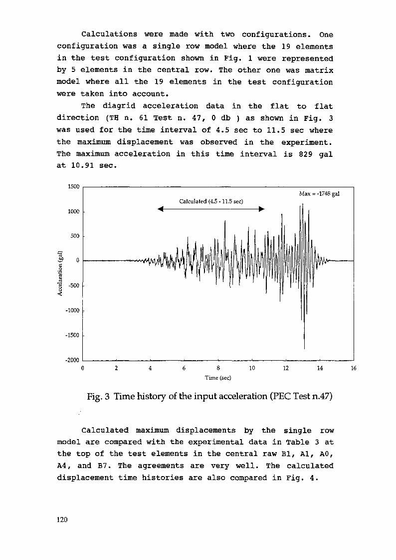
Calculations were made with two configurations. Oneconfiguration was a single row model where the 19 elementsin the test configuration shown in Fig. 1 were representedby 5 elements in the central row. The other one was matrixmodel where all the 19 elements in the test configurationwere taken into account.

The diagrid acceleration data in the flat to flatdirection (TH n. 61 Test n. 47, 0 db ) as shown in Fig. 3was used for the time interval of 4.5 sec to 11.5 sec wherethe maximum displacement was observed in the experiment.The maximum acceleration in this time interval is 829 galat 10.91 sec.

1500

1000 •

-2000

Fig. 3 Time history of the input acceleration (PEC Test n.47)

Calculated maximum displacements by the single rowmodel are compared with the experimental data in Table 3 atthe top of the test elements in the central raw Bl, Al, AO,A4, and B7. The agreements are very well. The calculateddisplacement time histories are also compared in Fig. 4.

120

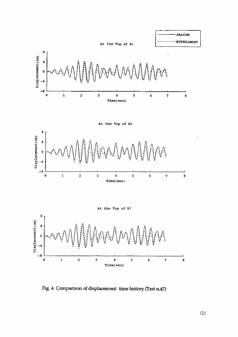
Displacement(cm)

SI OQ ft" n 1 s, È-. •a t» ET l f s

Dis

plac

emen

t cm

)

•8 0 Hi W

i i

00

*•

Dis

plac

emen

t(cm

)

to (t O

S ft if 0 Mi 9* o

I CO

to U)

ft if I 0 Ml

U

M

W

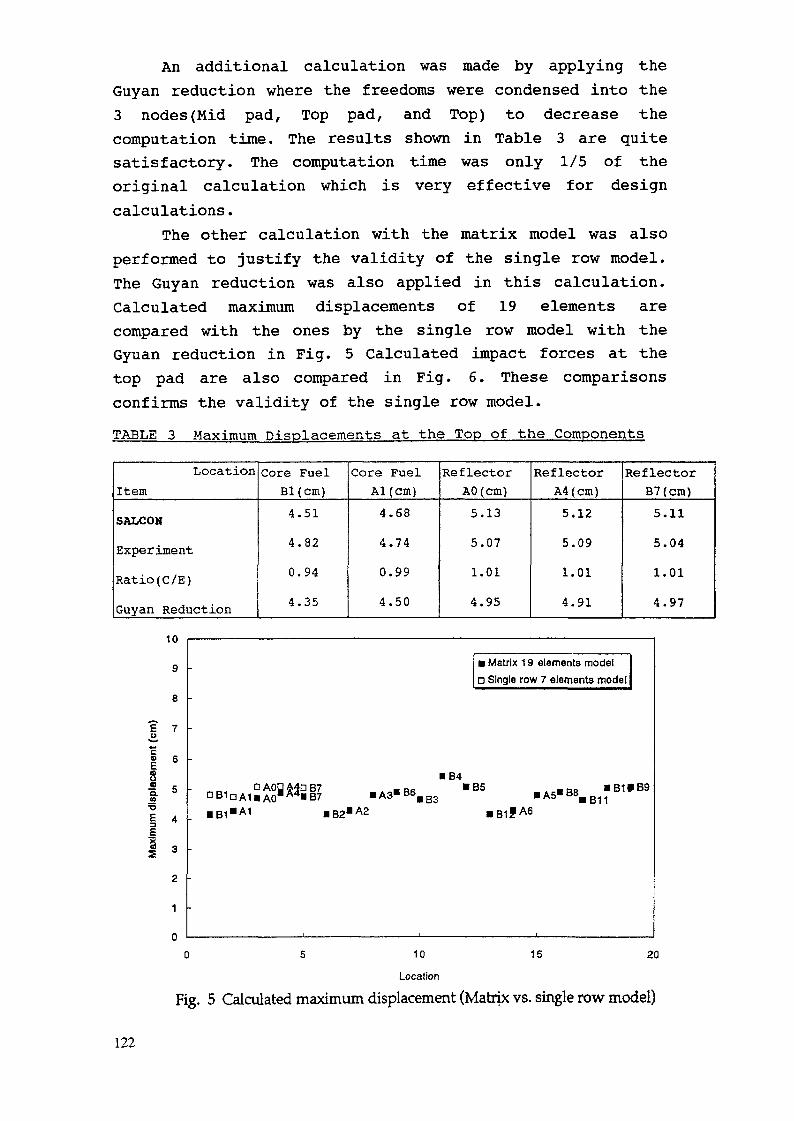
An additional calculation was made by applying theGuyan reduction where the freedoms were condensed into the3 nodes {Mid pad, Top pad, and Top) to decrease thecomputation time. The results shown in Table 3 are quitesatisfactory. The computation time was only 1/5 of theoriginal calculation which is very effective for designcalculations.

The other calculation with the matrix model was alsoperformed to justify the validity of the single row model.The Guyan reduction was also applied in this calculation.Calculated maximum displacements of 19 elements arecompared with the ones by the single row model with theGyuan reduction in Fig. 5 Calculated impact forces at thetop pad are also compared in Fig. 6. These comparisonsconfirms the validity of the single row model.TABLE 3 Maximum Displacements at the Top of the Components

LocationItemSALCON

ExperimentRatio (C/E)Guyan Reduction

Core FuelBl(cm)4.51

4.82

0.94

4.35

Core FuelAl(cm)4.684.74

0.994.50

ReflectorAO(cm)5.135.071.014.95

ReflectorA4 (cm)5.125.091.014.91

ReflectorB7(cm)5.115.041.014.97

Eu

B

lQ.

|

l

• Matrix 19 elements modelD Single row 7 elements model

• B4

• B1BA1 B2 A2 »BlfA6

10

Location

15 20

Fig. 5 Calculated maximum displacement (Matrix vs. single row model)

122

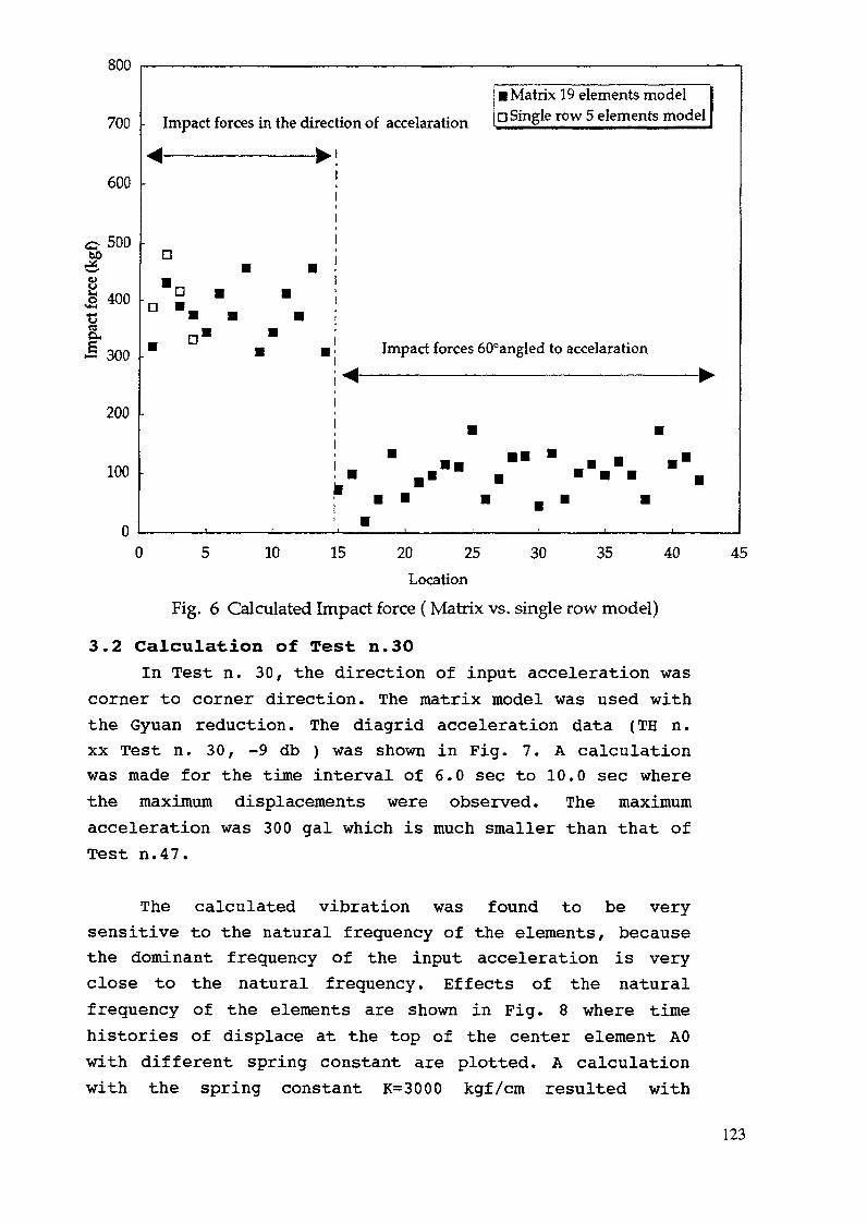
800

700

600

ooou

500

,0 400'SS-

>§ 300

200

100

0

Impact forces in the direction of accelaration

• Matrix 19 elements modelD Single row 5 elements model

D

n1Impact forces 60°angled to accelaration

0 10 15 30 35 4020 25Location

Fig. 6 Calculated Impact force ( Matrix vs. single row model)

3.2 Calculation of Test: n.30In Test n. 30, the direction of input acceleration was

corner to corner direction. The matrix model was used withthe Gyuan reduction. The diagrid acceleration data (TH n.xx Test n. 30, -9 db ) was shown in Fig. 7. A calculationwas made for the time interval of 6.0 sec to 10.0 sec wherethe maximum displacements were observed. The maximumacceleration was 300 gal which is much smaller than that ofTest n.47.

45

The calculated vibration was found to be verysensitive to the natural frequency of the elements, becausethe dominant frequency of the input acceleration is veryclose to the natural frequency. Effects of the naturalfrequency of the elements are shown in Fig. 8 where timehistories of displace at the top of the center element AOwith different spring constant are plotted. A calculationwith the spring constant K=3000 kgf/cm resulted with

123

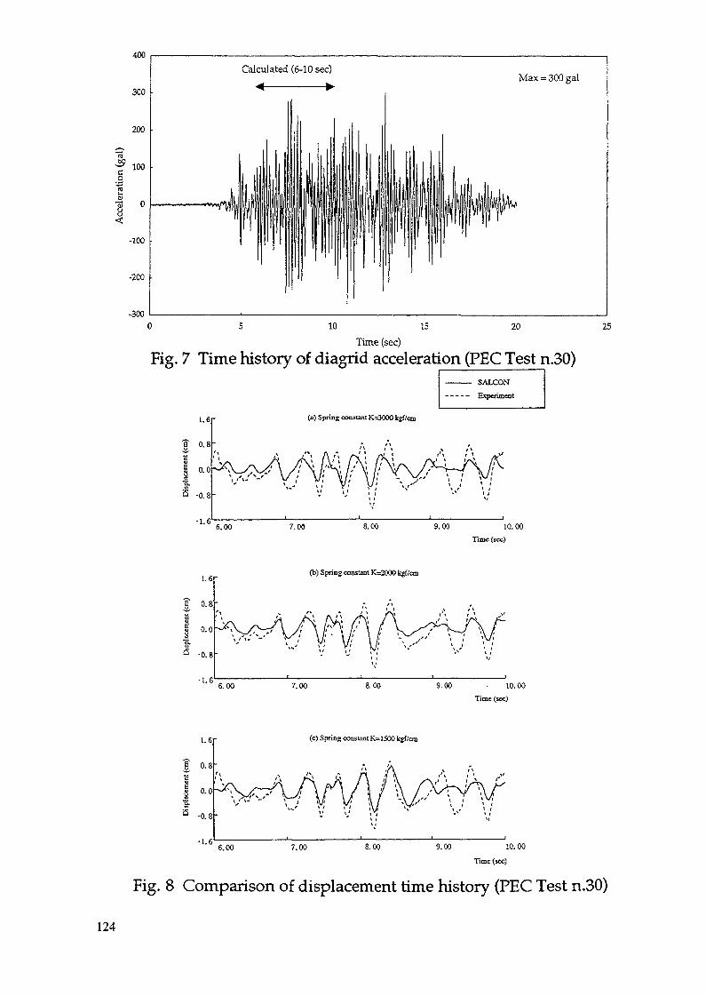
Time (sec)Fig. 7 Time history of diagrid acceleration (PEC Test n.30)

———— SALCON----- Experiment

1.6

0.8

(a) Spring constant K=3000 kgf/cm

6.00 7.00 9.00 10.00Time (sec)

1.6]

o.s:o.o

-0.8

-1.6 6.00

(b) Spring constant K=2000 kgf/cm

7.00 8.00 9.00 • 10.00Time (sec)

1.6]

0.0

-1.66.00

(c) Spring constant K=1500 kjf/on

7.00 8.00 9.00 10.00

Time (sec)

Fig. 8 Comparison of displacement time history (PEC Test n.30)

124

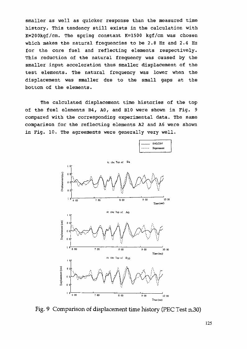
smaller as well as quicker response than the measured timehistory. This tendency still exists in the calculation withK=200kgf/cm. The spring constant K=1500 kgf/cm was chosenwhich makes the natural frequencies to be 2.8 Hz and 2.4 Hzfor the core fuel and reflecting elements respectively.This reduction of the natural frequency was caused by thesmaller input acceleration thus smaller displacement of thetest elements. The natural frequency was lower when thedisplacement was smaller due to the small gaps at thebottom of the elements.

The calculated displacement time histories of the topof the fuel elements B4, AO, and BIO were shown in Fig. 9compared with the corresponding experimental data. The samecomparison for the reflecting elements A2 and A6 were shownin Fig. 10. The agreements were generally very well.

SALOON

Expenment

It the Top of B4I 6r

6 00

At the Top of AO

0 8

1 6 6 00 7 00 i 00

At the Top of BIO

9 00 10 00Time (sec)

6 00 7 00 9 00 10 00Time (sec)

Fig. 9 Comparison of displacement time history (PEC Test n.30)

125

SALCONExperiment

At the Top of A2

1

i.er0.8

o.ojaCO

S -0.8

-1.6 6.00 7.00 8.00

At the Top of A6

9.00 10.00Time (sec)

1.6r

0.8

8 0.0!—O.

Ê -0.8

•1.6 6.00 7.00 8.00 9.00 10.00Time (sec)

Fig. 10 Comparison of displacement time history (PEC Test n.30)

4. Calculation of RAPSODZE TestsAs for RAPSODIE Tests RAP087 in the air and RAPZ32 in

the water, the seismic excitation of the test core wasrepresented by the central row which consists of 4nuetronic shield, 11 fuels and another 4 neutronic shields.Each of the 19 elements was modeled by 6 beams which werefixed at the bottom as shown in Fig. 11 and Fig. 12. Thefreedoms were condensed into the 3 nodes (Mid pad, Top pad,and Top) by Guyan reduction.

4.1 Calculation of Test RAP087The input data for RAP087 were summarized in Table 4.

The stiffness of the lower beam was adjusted to give thenatural frequency of 8 Hz for the fuel and 20 Hz for theneutron shield. At the top and middle pad levels, collision

126

elements were placed between each beams with the collisionrelated properties (spring/damping/gap) given in the dataprovided through IAEA. The fraction of critical damping forthe 1st vibration mode and the 2nd mode was 3% for thefuel and 1% for the neutron shield.

Impact ForceElement

HI-_j

Beam Stiffnesswas Adjusted

EL 1500 mm

EL 1280 mm

EL 995 nun

EL 710 mm

EL415mm

SALCON FEM MODEL

Y

A A

o00

V V

TEST FUEL ASSEMBLY

Fig.ll Calculation Model of Rapsodie Test Fuel Assembly

127

Impact ForceElement

Beam Stiffnesswas Adjusted

EL 1500 mm

EL 1280 mm

EL 995 mm

EL 710 mm

O EL 415 mm

O EL 120 mm

EL Omm

ooocs

SALCON FEM MODELTEST NEUTRONIC SHIELD

ELEMENT

Fig.12 Calculation Model of Rapsodie Test Neutronic Shield

A calculation was made during 0.15 to 2.65 sec of theinput acceleration shown in Fig. 10. The maximum inputacceleration was 1502.3 gal. The maximum displacements werecompared with the experimental data in Fig. 13. Thecalculated displacement time histories of the top of theelements were shown in Fig. 14 and Fig. 15 compared withthe corresponding experimental data. The displacement timehistories of the fuels were over plotted in Fig. 16compared with the experimental data. The agreements werereasonably well. The calculated maximum impact forces wereplotted in Fig. 17 and the typical time history wereplotted in Fig. 18.

128

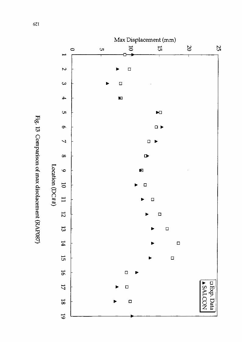
6ZI

3cw'*h-Aeuno3sua.03§SUX

s. n03£sun3fD

Ooo

K)

Öl

00

? «SUer.! s

K)

W

Öl

00

Max Displacement (mm)Öl Öl

D

IB

a

a

D

D >

E3

D

a

>• D

N3O

D

JS>Ul

> DW M

Z $

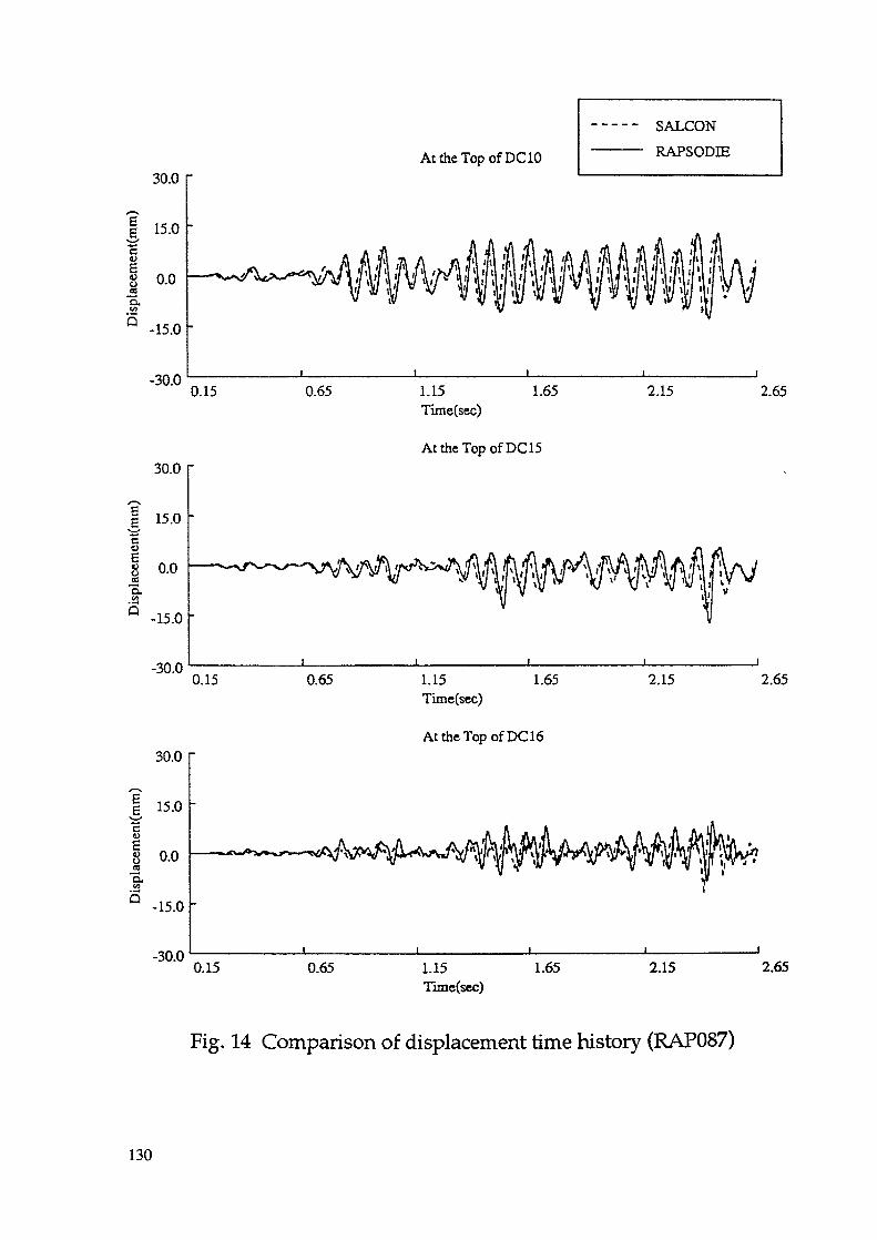
30.0

l 15.0eu

JS«9

S

o.o

-15.0

-30.0 0.15

30.0

l 15.0<u

o..säQ

0.0

-15.0

-30.00.15

30.0

l 15.0

i.

W

5 -15.0

-30.00.15

AttheTopofDCIO

----- SALCON———— RAPSODE

0.65 1.15Time(sec)

1.65 2.15 2.65

AttheTopofDCIS

0.65 1.15Time(sec)

1.65 2.15 2.65

AttheTopofDClö

0.65 1.15Time(sec)

1.65 2.15 2.65

Fig. 14 Comparison of displacement time history (RAP087)

130

30.0

l 15.0È:o

g 0.0o.u>2 -15.0

-30.00.15

30.0

§ 15.0

o

Cfl

"o.0.0

-15.0

-30.00.15

30.0

I 15.0c

1 o.oofQ.v>5 -15.0

-30.00.15

0.65

0.65

At the Top of DCO1

1.15Time(sec)

1.65

AttheTopofDC04

1.15Time(sec)

1.65

AttheTopofDC05

----- SALCONRAPSODffi

2.15 2.65

2.15 2.65

0.65 1.15Time(sec)

1.65 2.15 2.65

Fig. 15 Comparison of displacement time history (PAP087)

131

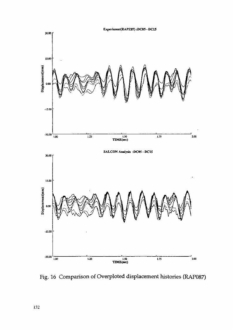
30.00 rExperiment(RAPZ87) -JÎC05 - DC15

15.00

-30.001.50

TIME(sec)1.75 2.00

30.00 r

13.00

BB

BZer

lQ

0.00

-15.00

-30.00

SALCON Analysis :DC«5 - DC15

1.00 L25 1.50TIME(sec)

1.75 2.00

Fig. 16 Comparison of Overploted displacement histories (RAP087)

132

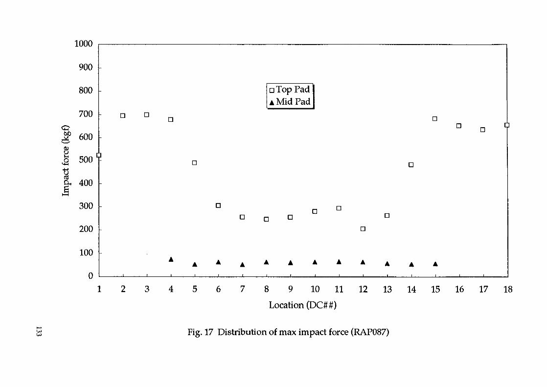
•8

1000

900

800

700

600

500

400

300

200

100

0

p

D O

i_______i

D

D

D

D OD D

D

D

D

D

D

l 2 3 4 5 6 7 8 9 10 11 12 13 14 15 16 17 18Location (DC##)

Fig. 17 Distribution of max impact force (RAP087)

loo.o r

Ioex

M

75.0

50.0

25.0

0.0L i l i l L

0.15 0.65

At the Mid Pad of DC05

1.15Time(sec)

1.65

SALCON

2.15 2.65

100.0 T

0.15

At the Mid Pad of DC07

0.65 1.15Tlme(scc)

1.65 2.15 2.65

loo.o rAt the Mid Pad of DCIO

J*N—S

8

äCL£

75.0

50.0

25.0

0.00.15 0.65 1.15

Tïme(sec)1.65 2.15 2.65

Fig. 18 Time histories of impact force (RAP087)

134

4.2 Calculation of Test RAPZ32As for Test RAPZ32 in the water, calculations were

made with the single row model. The effects of fluid wastreated by add mass. In order to decrease the naturalfrequency by 15% as described in the provided data, the addmass should be 2.5 times the fluid displacement mass asshown in Table 5. in the reference case, the large add masssuppresses the effective input acceleration by the factorßf as shown in Table 5. The calculated maximum displacementwith the reference input data was much smaller than theexperimental data as shown in Fig. 19. Two additionalcalculations were made to modify the effects of fluid. Thecalculation with smaller add mass (CASE A),thus larger ßfcan give the displacement comparable to the experimentaldata. The other one (CASE B) was neglecting thedisplacement mass which also increases ßf than thereference case. Moreover the stiffness of the neutronicshield was modified in the both cases as some problem inthe boundary condition was reported^). Although more workis needed to evaluate the effects of fluid, the agreementsare most satisfactory. The displacement time histories ofthe fuels were over plotted in Fig. 20.

5. Calculation of Monju testsMonju test has been calculated by SALCON code. The

followings are some results from open literature )The calculation model for the Monju single row test

and its input acceleration normalized to 400 gal are shownin Fig. 21 and 22 respectively. The calculated maximumdisplacements and some of their time histories are plottedin Fig. 23 together with the experimental data. Theagreements are satisfactory. As for the Monju matrix test,the single row model was used as shown in Fig. 24. Theinput acceleration was normalized to 600 gal. The maximumdisplacements and the time history of left most(No.l)assembly are compared with their respective experimentaldata in Fig. 25. The agreements are generally good.

135

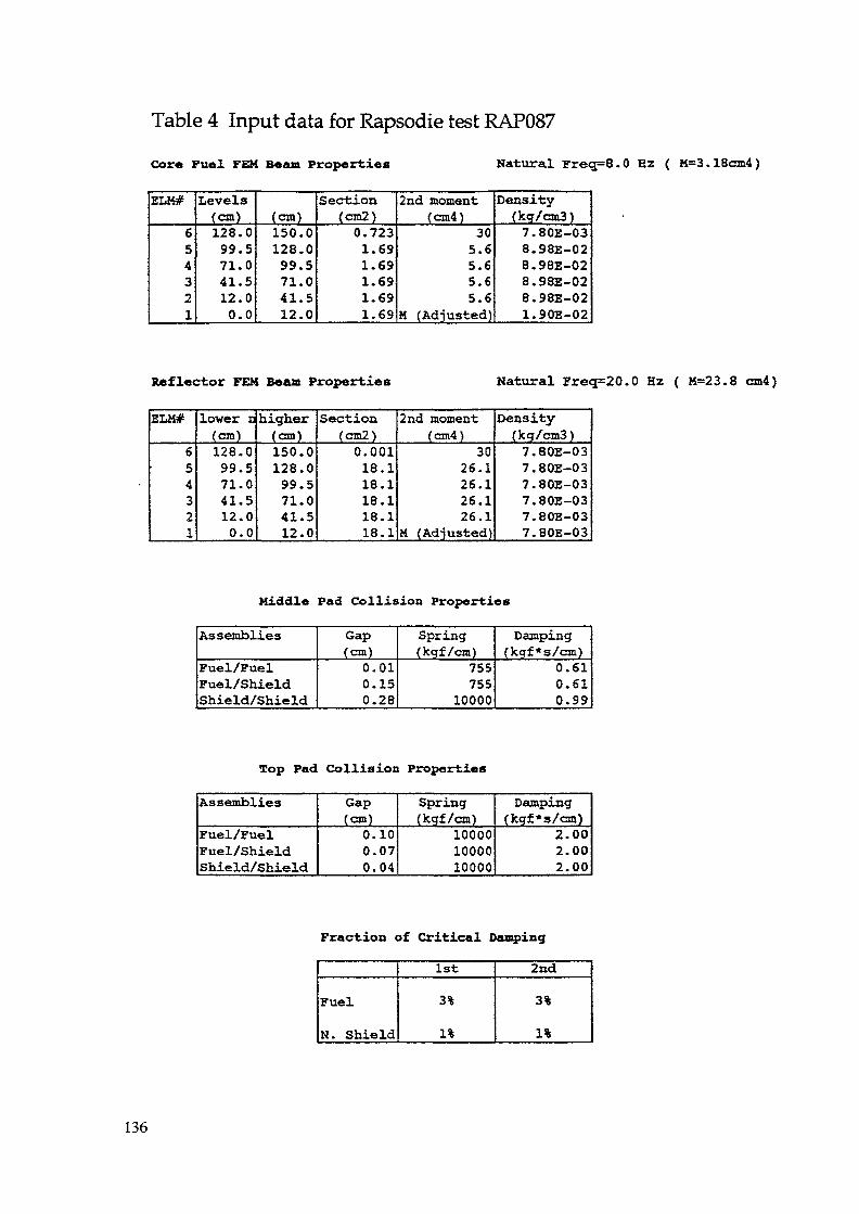
Table 4 Input data for Rapsodie test RAP087

Cor« Fuel FEM Bean Proper-ties Natural Freq=8.0 Hz ( M=3.18cm4)

ELM#

654321

Levels(cm)128.099.571.041.512.00.0

(cm)150.0128.099.571.041.512.0

Section(cm2)0.7231.691.691.691.691.69

2nd moment(cm4)

305.65.65.65.6

M (Adjusted)

Density(kg/cm3)7.80E-038.98E-028.98E-028.98E-028.98E-021.90E-02

Reflector FEH Beaut Properties Natural Freq=20.0 Hz ( M=23.8 cm4)

2LM#

654321

lower a(cm)128.099.571.041.512.00.0

higher(cm)150.0128.099.571.041.512.0

Section(cm2)

0.00118.118.118.118.118.1

2nd moment(cm4)

3026.126.126.126.1

M (Adjusted)

Density(kg/cm3)7.80E-037.80E-037.80E-037.80E-037.80E-037.80E-03

Middle Pad Collision Proper-ties

AssembliesFuel/FuelFuel/ShieldShield/Shield

Gap(cm)

0.010.150.28

Spring(kgf/cm)

755755

10000

Damping(kgf*s/cm)

0.610.610.99

Top Pad Collision Properties

Assemblies

Fuel/FuelFuel/ShieldShield/Shield

Gap(cm)

0.100.070.04

Spring(kgf/cm)

100001000010000

Damping(kgf*s/cm)

2.002.002.00

Fraction of Critical Damping

Fuel

N. Shield

1st

3%

1%

2nd

3%

1%

136

Table 5 Parameters for Calculations of RAPZ32 Test

"\Reference

CASE A

CASE B

Fluid EffectsCf

2.5

1.0

2.5

ßf (Fuel)

0.64

0.76

0.72*

Natural frequencyFuel Assem.

6.84 Hz

7.47 Hz

7.47 Hz

N. Shield

17.4 Hz

15.5 Hz**

12.5 Hz**

Fraction of Critical DampingFuel Assem.

5.0%

5.0%

5.0%

N. Shield

3.0%

3.0%

3.0%

Note:M-Mj =0.0 ** Stiffness was modified

U)-o

Mff: Fluid Add Mass

M^: Fluid Displacement Mass Md = S-pw

where S: Cross Section of the Displaced Fluid

/V Density of Fluid (water)

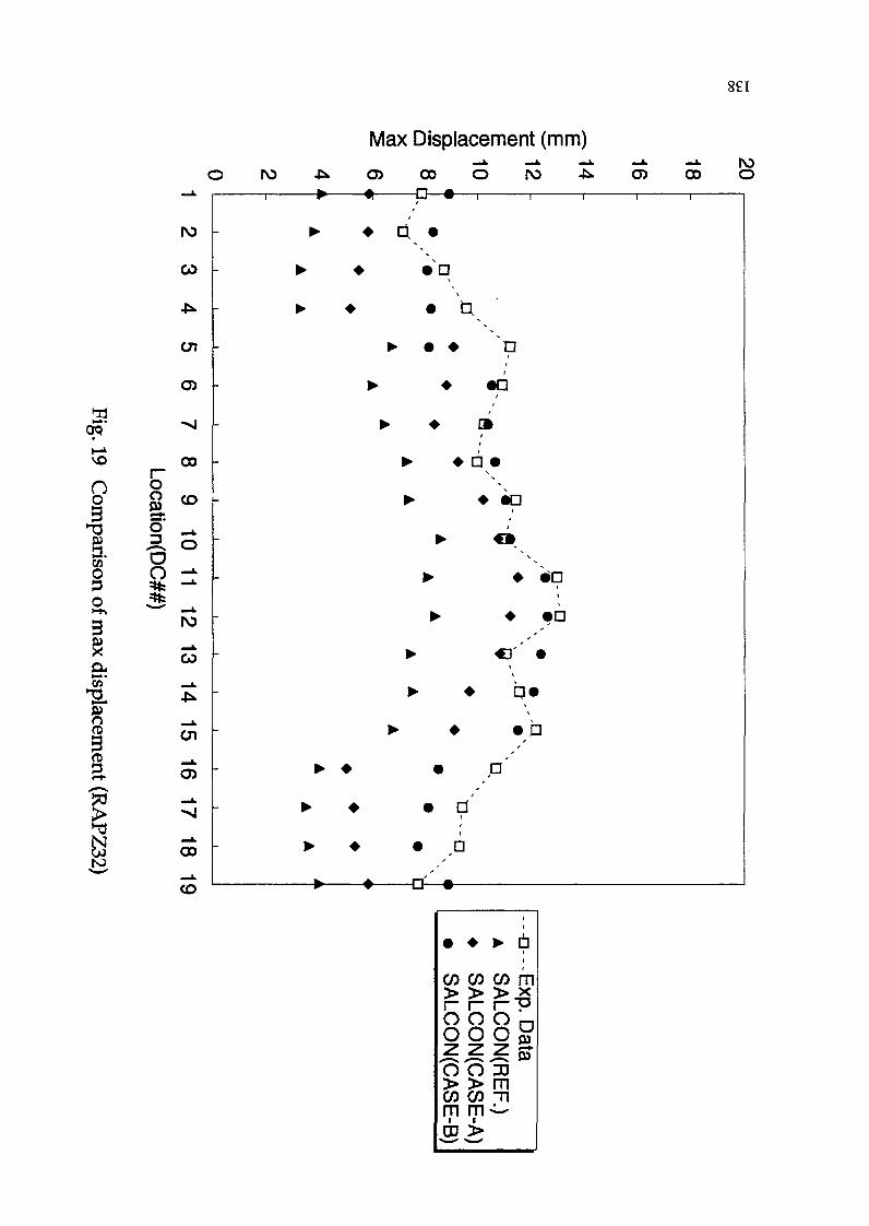
8£l

Max Displacement (mm)

OP

en§

et55'STn

CO

en

o

co

O toja ***

5' _,.>=3. oOO ^

IV)

co

en

oo

co

-o—•-* d, •* «n

• «a

' ** È*

• «a

ci' •* g*

diD

-D - -

co co co m> > >><O O O nO O O ojZ 2^ $O O DO> > mCO CO Tlm rn

N>o

O)

«J

û

30.00

25.00

20.00

15.00

10.00

5.00

0.00

•5.00

•10.00

8018018058068078088098108118128138H815816819

•15.00 1.00 1.50 2. 00 2. 50Time (sec)

3.00 3.50 4.00

Fig. 20 Overplot of calcurated displacement histories (RAPZ32)

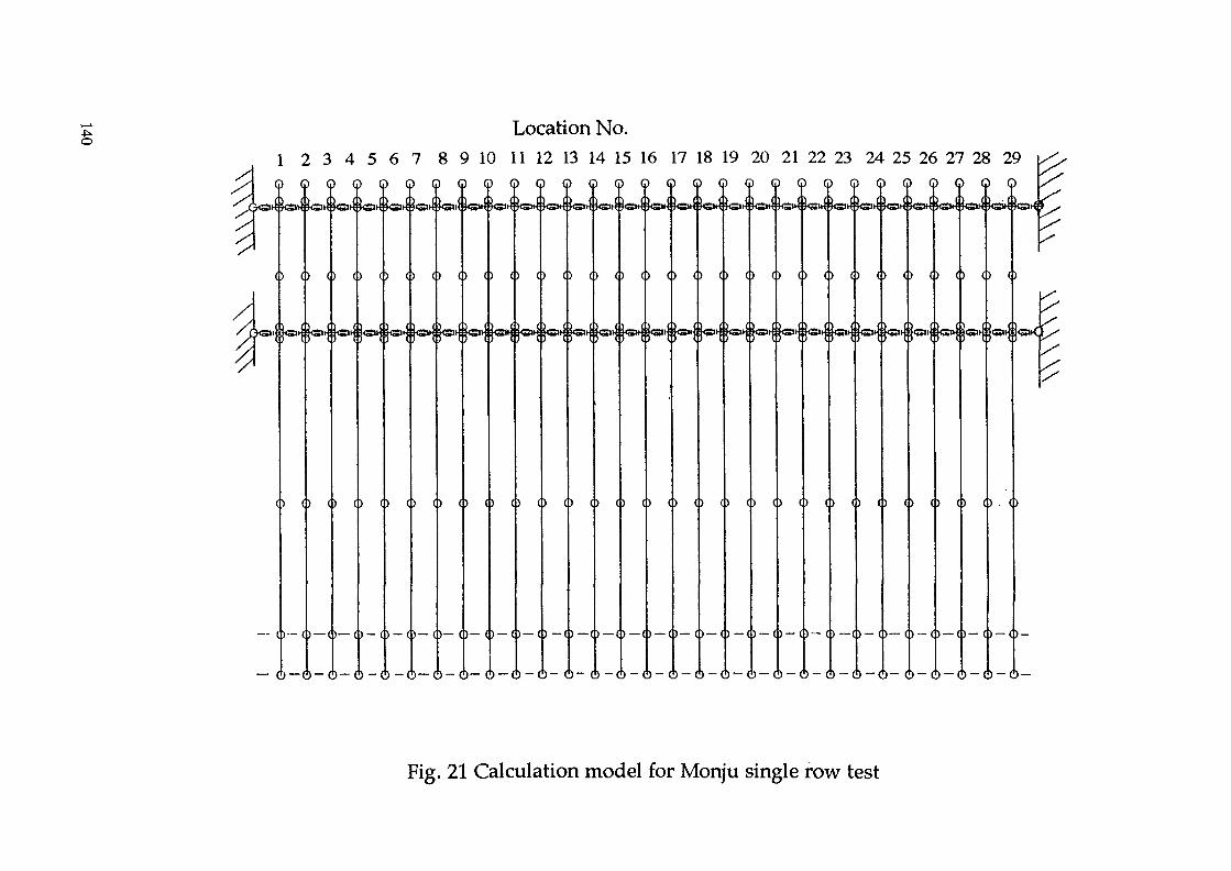
Location No.1 2 3 4 5 6 7 8 9 10 11 12 13 14 15 16 17 18 19 20 21 22 23 24 25 26 27 28 29

X

^

(

<

— 1

(M

(

1 I

)— (

> — r

) (<SF|

H

> (

i— f

> <

H

> c

>— f

> c(.„n, (

H

)— (> — f

> c

i (

> <

> — c> — f

> «1 L

") (

N

> <

i — i

(<5>K

H

> <

> — <> — «

) ««S»k

N

> <

>— f

) (

N

> (

) — C

> — f

(«l»i

M

> (

)— C

) — f

(k^

H

) (

) — (

)— f

) (ks.4

N

> «

)— c> — f

t•;CT,i

> (

H

> (

> — C

) — f

(

H

> <

> — c> — t

> <

H

> (

> — c> - f

(

*\tm**\

>— C

) — f

) (

H

> f

)— C

> — (

(

Iri4^oëin

) {

) — C

)— f

) (

) (><B»ttX

1 (

1—— 1

(

.4

) (

H

) C

) — C

) (<»4

> <

H

) <

)— c>- c

cw

> t

H

> <

(:i 4

H

)— C

) (W

H

)— f

> (^

H

> <

) — C

)— f

(^

) (

1 _ J

) (

)— C

) — f

(M

) (

M

>— c5 — C

(

*o4

(

H

> — (

Fig. 21 Calculation model for Monju single row test

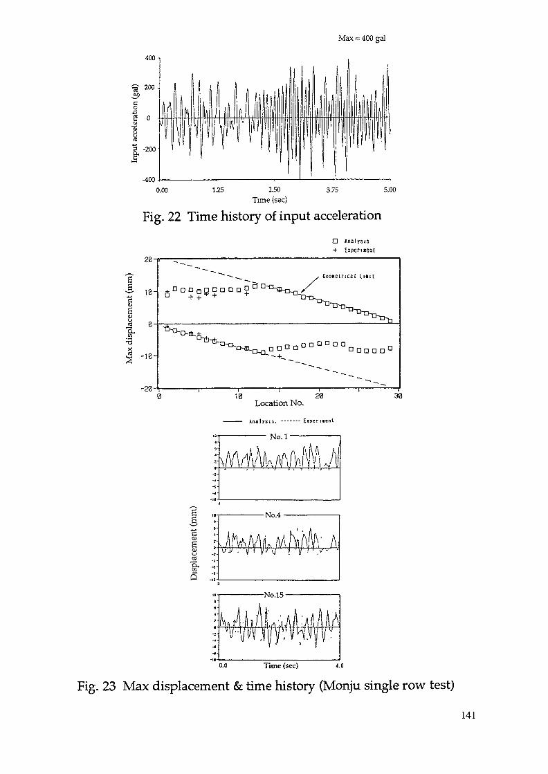
ho

Max

dis

plac

emen

t (m

m)

&In

put a

ccel

erat

ion

(gal)

tf. B S- &

C3 18

D

l EL

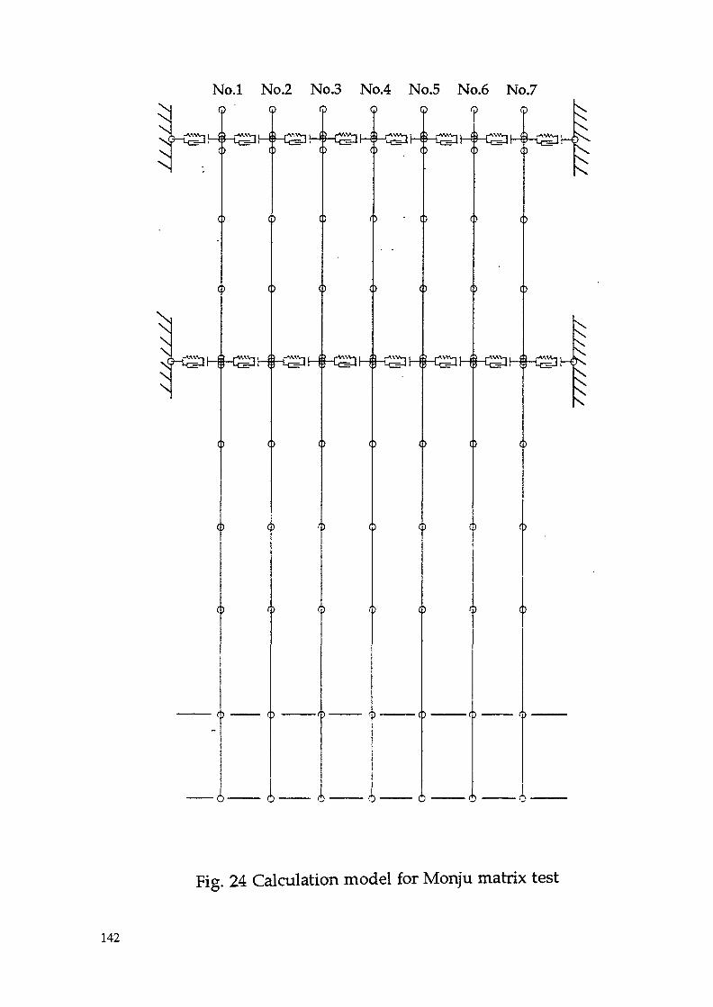
X]XX

X

X\XX

No.l No.2 No.3 No.4 No.5 No.6 No.7Q ' Q O Q Q Q Q

C)

C )

O

( ) C )

O ( ) <) <>

C)

f ) ————O

Q m

( > C)

O

X

XX

XX

Fig. 24 Calculation model for Monju matrix test

142

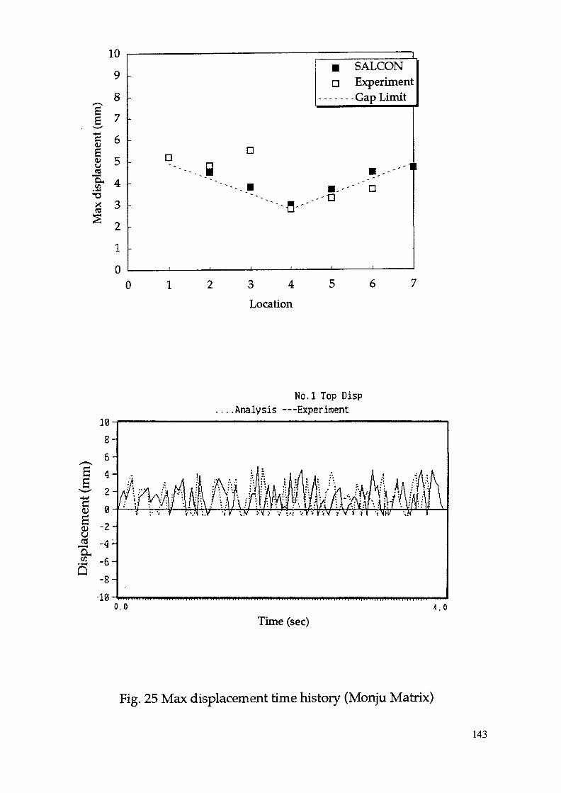
Disp

lace

men

t (m

m)

a K) i a n ro er. n> cn' I ? X

H re ft> o

Max

disp

lace

men

t (m

m)

r R »>

Ul ON

D

•D

D

Ü

O

D ill

||8

ë.

(Î

Zr*

3

U)

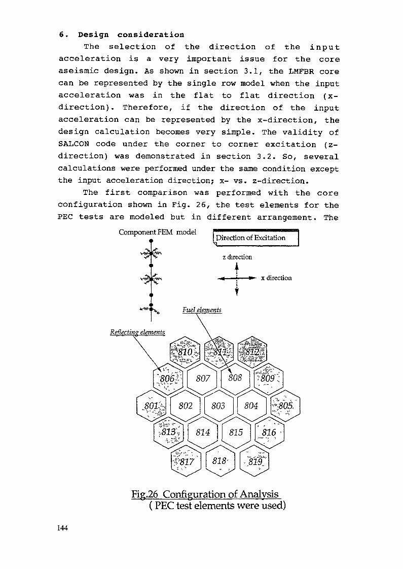
6. Design considerationThe selection of the direction of the input

acceleration is a very important issue for the coreaseismic design. As shown in section 3.1, the LMFBR corecan be represented by the single row model when the inputacceleration was in the flat to flat direction (x-direction). Therefore, if the direction of the inputacceleration can be represented by the x-direction, thedesign calculation becomes very simple. The validity ofSALCON code under the corner to corner excitation (z-direction) was demonstrated in section 3.2. So, severalcalculations were performed under the same condition exceptthe input acceleration direction; x- vs. z-direction.

The first comparison was performed with the coreconfiguration shown in Fig. 26, the test elements for thePEC tests are modeled but in different arrangement. The

Component FEM modelDirection of Excitation

z directioni

- »• x direction

Fuel elements

Reflecting elements

•¥817 818- . 819

Fig.26 Configuration of Analysis( PEC test elements were used)

144

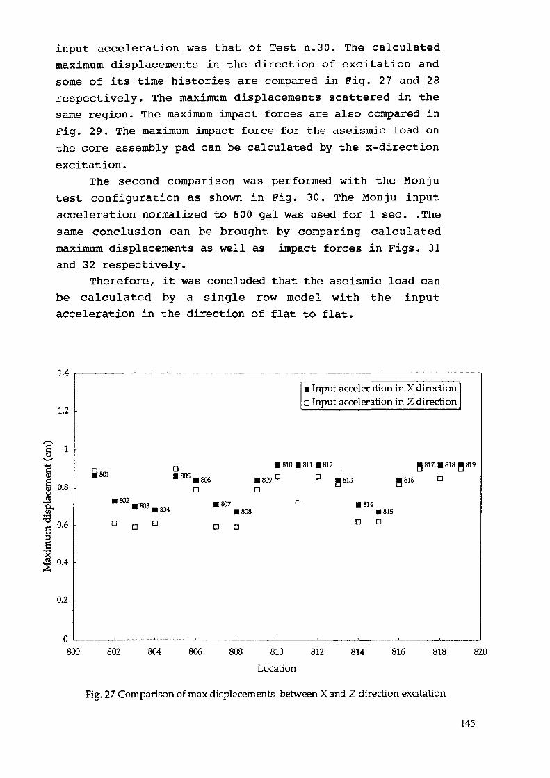
input acceleration was that of Test n.30. The calculatedmaximum displacements in the direction of excitation andsome of its time histories are compared in Fig. 27 and 28respectively. The maximum displacements scattered in thesame region. The maximum impact forces are also compared inFig. 29. The maximum impact force for the aseismic load onthe core assembly pad can be calculated by the x-directionexcitation.

The second comparison was performed with the Monjutest configuration as shown in Fig. 30. The Monju inputacceleration normalized to 600 gal was used for 1 sec. .Thesame conclusion can be brought by comparing calculatedmaximum displacements as well as impact forces in Figs. 31and 32 respectively.

Therefore, it was concluded that the aseismic load canbe calculated by a single row model with the inputacceleration in the direction of flat to flat.

1.4

1.2

• Input acceleration in X directiong Input acceleration in Z direction

cO>

rt

3

810 • 811 • 812 H 817 • 818 R 819

809°O D

I805H806 •809° D g 813 p 816

1802 • 807 D 1814• 808 • 815

D DD D

0.4

0.2

0800 802 804 806 808 810 812 814 816 818 820

Location

Fig. 27 Comparison of max displacements between X and Z direction excitation

145

Disp

lacem

ent (

cm)

Disp

lacem

ent (

cm)

Disp

lace

men

t (cm

)

3 CTQ £ ! B. co § n Si- tu ff a CO u su 8 <D 3- er. 3 o 3T & ^

. o o o o

i'

p O

p O>

o o

•8 00 g

o o

i'

p Op o

p o>

o o o o

ET n> •t O •o o •- 00

o o

51•o 00 o t\3

O O

oJP1a,S

H- *

90

80

70

60

50

40

30

20

10

0

• Input acceleratia Input accelerati

-

•

.

• • nB • n D

• • "" n D

D D DD G °° D

on in X directionon in Z direction

nn

Ü D

a°D

D D DD

LocationFig. 29 Comparison of impact forces between X and Z direction excitation

z direction

—*• x direction

Fig. 30 Configuration of Analysis( Monju assemblies were used)

147

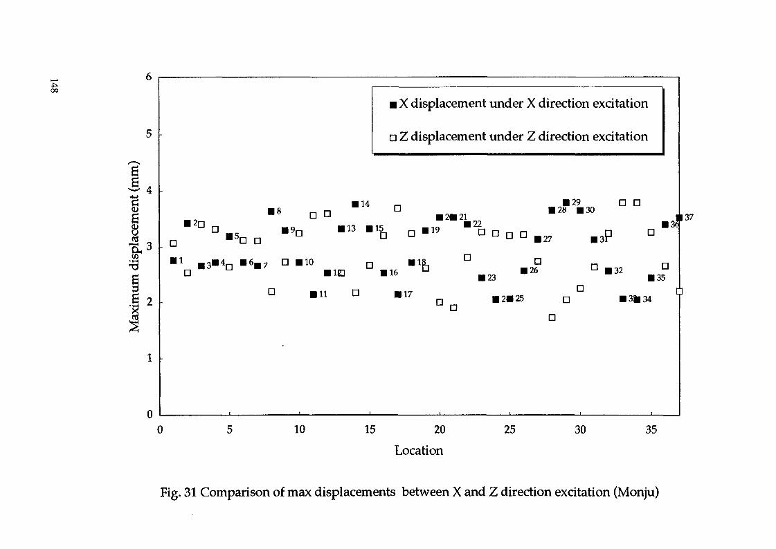
00

^ -Xgs>*t* '•Ma0)i

.1 2

0

I2rj

• X displacement under X direction excitation

ö Z displacement under Z direction excitation

114D 12« 21

• 29 D ö128 B30

113 mi5a Q B19 122137

o a ö 127D

O .„ D

D

• IQ

111 d• 23

a126 D «32 D

135

117 DD D B3»34

D

0 10 15 20

Location25 30 35

Fig. 31 Comparison of max displacements between X and Z direction excitation (Monju)

6000

5000

4000c-tf

j) 3000tjCuS"" 2000

1000

• Impact forces under X direction excitationD Impact forces under Z direction excitation

D

G

• a

,n aen

D

D •0

a D a a

a aa ü ,-,

20 40 60 80

Location100 120 140

Fig. 32 Comparison of impact forces between X and Z direction excitation (Monju)

Reference

1) Y. Sasaki, étal.,'Experimental Studies on Seismicvibration Phenomena of FBR Core Components',SMiRT7,F7/3,1983

2) Y. Sasaki, etal.,'Seismic Analysis of LMFBR CoreComponents',SMiRT 11,216/3, 1991

3) H.M.Hubert,T.J.R. Hughes etal.,'Improved NumericalDissipation for the Time Integration Algorithms inStructual Dynamics', Earthquake Eng. and structuralDynamics, Vol. 5, p283,1977

4) R.J. Guyan,'Reduction of Stiffness and Mass Matrix1,AIAAJ. Vol 3, p380, 1985

Next page(s) left blank 149

ANALYSIS OF THE CORE SEISMIC EXPERIMENTSUSING THE SAFA PROGRAM FOR INTERCOMPARISONOF LMFBR SEISMIC ANALYSIS CODES

T. HORIUCHIMechanical Engineering Research Laboratory,Hitachi Ltd,Tsuchiura, Ibaraki,Japan

Abstract

As a project of the IAEA/IWGFR, a coordinated research program on intercomparison ofLMFBR seismic analysis codes has been undertaken since 1991. In this research program, theparticipants conducted calculations on PEC, MONJU and RAPSODIE problems using theirown computer programs. As a final report for the coordinated research program, the resultscalculated using the SAFA program developed by Hitachi, Ltd. are reviewed. Since the calcula-tion results were found to correlate well with the ones measured during comparisons, the validityof SAFA for the seismic-response analysis of an FBR core was demonstrated. Intercomparisonof computer codes and some recommendations for future research are also made.

1 Introduction

A coordinated research program (CRP) on the intercomparison of LMFBR seismic analysis codeshas been undertaken since 1991 as a project of IAEA/IWGFR. The experimental data listed belowcontributed as problems for the coordinated research program.

• PEC — 19 elements in a matrix [1]

• RAPSODIE — 291 elements in a matrix [2]

• MONJU — 29 elements in a single row and 37 elements in a matrix [3] [4]

This paper has been prepared as a final report for the coordinated research program, in whichthe following is contained:

1. State-of-the-art in this field,

2. Description of the SAFA program, developed by Hitachi, Ltd., to analyze core componentvibration of fast breeder reactor core components during seismic excitation, and used for thebenchmark analyses in this CRP,

3. Review of results calculated using the SAFA program,

4. Intercomparison of computer codes,

5. Recommendations for future research.

2 State-of-the-art experimental and analytical work2.1 Overview

A fast breeder reactor (FBR) core is composed of as many as one thousand core components, includ-ing fuel assemblies, blanket assemblies, and neutron shield assemblies, all of which are immersed ina coolant fluid (liquid sodium). The subassemblies have load pads that transfer contact forces toadjacent subassemblies. When an earthquake excites the structure, these structural characteristics

151

cause the subassemblies to vibrate like cantilevers with load pad impacts under fluid-structure in-teraction. Since the seismic integrity of the core components is an important factor in FBR design,various studies have been made on the development and testing of seismic analysis codes for FBRcores. These are reviewed in this section.

The studies mainly focuse upon the following items:

1. Modeling fluid interaction forces,

2. Dealing with large number of degrees of freedom,

3. Integrating equation of motion with respect to time,

4. Determining nonlinear forces caused by impacts.

It is important to consider all of these items when simulating the seismic responses of structuralcharacteristics.

2.2 Experiments

Fundamental experiments on the evaluation of fluid force acting on subassemblies were conductedby Fujita[5], Preumont, et al.[6], and Horiuchi, et al.[7]. Vibration characteristics of a group ofbars installed in a small gap were experimented on by Horiuchi, et al.[8]. These results were usedto develop e and improve analytical and computational approaches.

Several experiments simulating actual FBR core structures have also been reported. Sasaki andMuto reported on experiments using MONJU (Japanese prototype reactor) core components[9].Martelli, et al. discussed experiments using PEC (Italian experimental reactor)[10]. Brochard, et al.reported results of experiments using a mock-up of RAPSODIE (French experimental reactor)[ll].

The MONJU experiments were conducted in air and in water using life-size subassembly modelsinstalled on a shaking table with two types of set-ups, that is, 29 bars in a single row and 37 barsarranged in a hexagonal matrix. Throughout the experiments, vibration characteristics such asresonant frequencies were measured as well as the time histories of displacement response, impactforce, and strain.

In the PEC experiments, up to 19 subassemblies in various set-ups were excited using a shakingtable with earthquake or random waves. The displacement responses were measured.

In the RAPSODIE experiments, the core model was composed of 91 fuel-assembly models (thecenter plus 5 rings) and 181 neutron shield models (4 rings). The displacement responses for anearthquake wave were recorded.

These experimental results contribute not only in showing the integrity of the structural designbut also in validating seismic-analysis computer codes. These data have also been utilized asproblems for this CRP of intercomparison work of LMFBR seismic analysis codes.

2.3 AnalysisIn addition to experimental work, studies on developing seismic-response-analysis methods andcomputer codes are being conducted in accordance with FBR development. In computer codes forseismic response analysis, subassemblies are usually modeled using beam finite-elements, and animpact phenomenon is described with a set comprised of a spring, a damper, and a gap.

Preumont, et al. developed a program named CLASH and calculated of SNR-2 plant seismicresponse [12]. This program treats any impact force as a pseudo-external force and a fluid force asa concentrated added mass. It is capable of calculating the seismic response of the core in two-dimensional arrangements. Martelli made use of a computer code named CORALIE to analyzeseismic responses in the PEC experiment discussed earlier[10]. This computer code can evaluatethe response of one-dimensional core model. Brochard, et al. also calculated for the RAPSODIEexperiment using CORALIE[13]. Morishita, et al. used a general-purpose finite-element-method

152

program, FINAS, to calculate the results obtained from the MONJU experiments[14]. Sasaki, et al.also conducted MONJU analysis using the Guyan reduction[15] in limiting the number of degreesof freedom[16]. Horiuchi, et al. developed a computer program named SAFA to analyze the seismicresponse of FBR core components[17]. The program was verified by comparisons with experimentalresults.

2.4 Response in the vertical direction

An evaluation of the vertical response of subassemblies is also important for structural design.Studies for this purpose were made by Aida, et al. [18] and Amada, et al. [19].

3 Description of core seismic analysis code

Benchmark analysis to be discussed in the following was performed using the SAFA (SeismicAnalysis program for Fuel Assemblies) computer program, developed by Hitachi, Ltd. to analyzecore component vibration in fast breeder reactors (FBR) during seismic excitation. The featuresof SAFA are briefly described as follows. Detailed discussion on the computer program has beenreported elsewhere [17].

3.1 Consideration of fluid force

Fluid force is considered as added mass in SAFA because fluid force is approximately proportionalto the acceleration of structures. Using this assumption, the equation of motion becomes

(M + My) x + Cx + Kx + q = -/, (1)

where M and Mv are mass and added mass matrices, respectively, C is a damping matrix, K isa stiffness matrix, x is a relative displacement vector, / is the earthquake-generated external forcevector, and q is the impact force vector.

Two types of added mass may be selected. One is a three-dimensional added mass matrix, usingwhich the interaction between the subassemblies and the core barrel, due to fluid force, is able tobe precisely considered. Although the added-mass matrix can be calculated by using another FEMcode, the calculation requires so much memory and so much computational time that the numberof degrees of freedom (DOFs) is limited at present. However, further improvements in calculationmethods and computer technology are expected to allow us to calculate the actual size of FBRcore structures. The other type of added mass is a concentrated added mass. This is a simplifiedmethod to treat fluid structure interaction, by which the natural frequency of the first mode ofthe subassemblies can be simulated. This allows seismic response to be calculated to a certainaccuracy when concentrated added mass is properly defined, because the first natural frequency isan important factor in the seismic response of subassemblies. Several methods to determine theadded mass based on structural conditions have been proposed [20] [7].

3.2 Reduction in the number of degrees of freedom

The modal superposition method [21] was employed by SAFA to transfer the coupled multi-degree-of-freedom system described by Eq. (1) to a set of single-degree-of-freedom (SDOF) systems inmodal space. The time integration of the equations of motion was then conducted in modal spaceand the SDOF system responses were transformed back to the original space to determine theseismic responses of the subassemblies.

Although as many eigen modes as the number of the system DOFs can be determined by modalanalysis, some of the modes contribute little to seismic response. These modes have therefore beeneliminated in the calculation to reduce the number of DOFs, to reduce computation time.

153

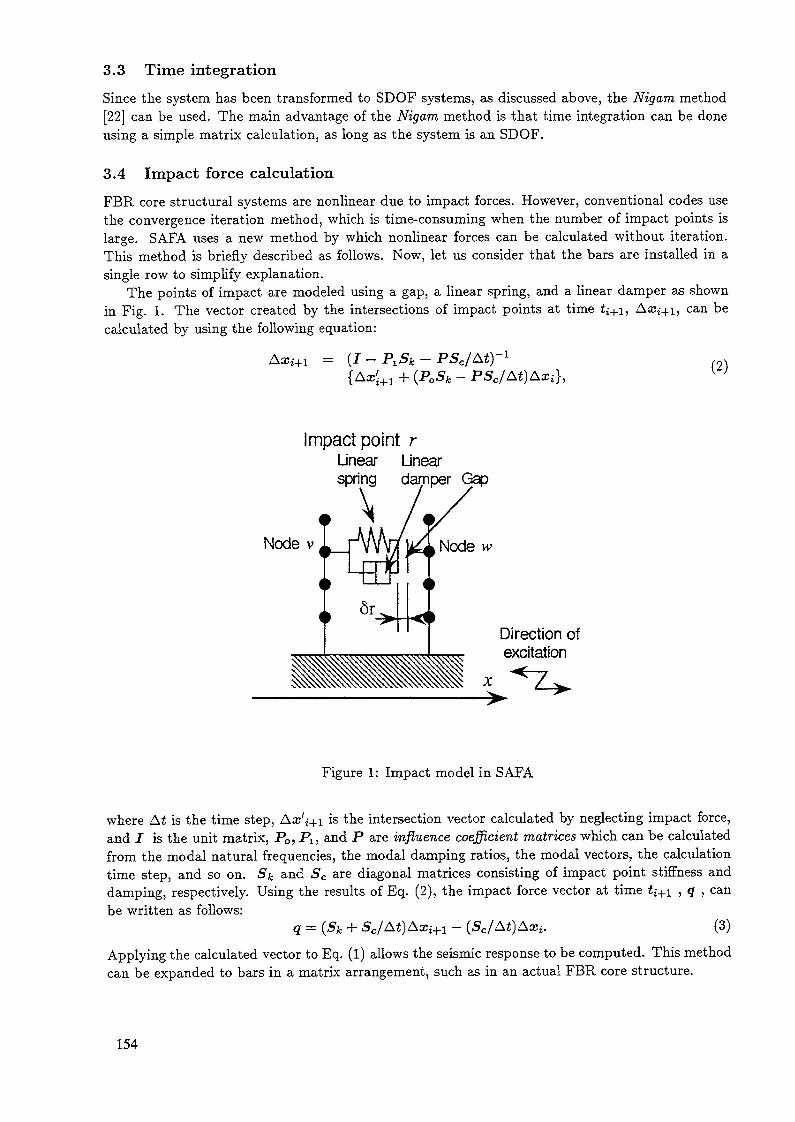
3.3 Time integration

Since the system has been transformed to SDOF systems, as discussed above, the Nigam method[22] can be used. The main advantage of the Nigam method is that time integration can be doneusing a simple matrix calculation, as long as the system is an SDOF.

3.4 Impact force calculation

FBR core structural systems are nonlinear due to impact forces. However, conventional codes usethe convergence iteration method, which is time-consuming when the number of impact points islarge. SAFA uses a new method by which nonlinear forces can be calculated without iteration.This method is briefly described as follows. Now, let us consider that the bars are installed in asingle row to simplify explanation.

The points of impact are modeled using a gap, a linear spring, and a linear damper as shownin Fig. 1. The vector created by the intersections of impact points at time ti+i, Axj+i, can becalculated by using the following equation:

= (I - k - P5C/ At)-1

(P0Sfc - (2)

Impact point rLinear Linearspring damper Gap

Node v Node w

Direction ofexcitation

Figure 1: Impact model in SAFA

where Ai is the time step, Ax'i+i is the intersection vector calculated by neglecting impact force,and J is the unit matrix, P0, PI, and P are influence coefficient matrices which can be calculatedfrom the modal natural frequencies, the modal damping ratios, the modal vectors, the calculationtime step, and so on. Sfc and Sc are diagonal matrices consisting of impact point stiffness anddamping, respectively. Using the results of Eq. (2), the impact force vector at time ij+i , q , canbe written as follows:

q = (Sk + Sc/At)A»i+1 - (5c/At)Axi. (3)

Applying the calculated vector to Eq. (1) allows the seismic response to be computed. This methodcan be expanded to bars in a matrix arrangement, such as in an actual FBR core structure.

154

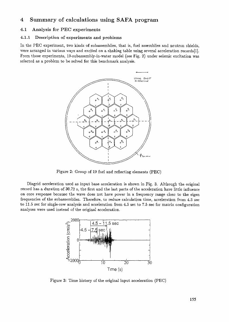
4 Summary of calculations using SAFA program

4.1 Analysis for PEC experiments

4.1.1 Description of experiments and problems

In the PEC experiment, two kinds of subassemblies, that is, fuel assemblies and neutron shields,were arranged in various ways and excited on a shaking table using several acceleration records [1].From those experiments, 19-subassembly-in-water model (see Fig. 2) under seismic excitation wasselected as a problem to be solved for this benchmark analysis.

Figure 2: Group of 19 fuel and reflecting elements (PEC)

Diagrid acceleration used as input base acceleration is shown in Fig. 3. Although the originalrecord has a duration of 30.72 s, the first and the last parts of the acceleration have little influenceon core response because the wave does not have power in a frequency range close to the eigenfrequencies of the subassemblies. Therefore, to reduce calculation time, acceleration from 4.5 secto 11.5 sec for single-row analysis and acceleration from 4.5 sec to 7.5 sec for matrix configurationanalyses were used instead of the original acceleration.

2000

Time (s)

Figure 3: Time history of the original input acceleration (PEC)

155

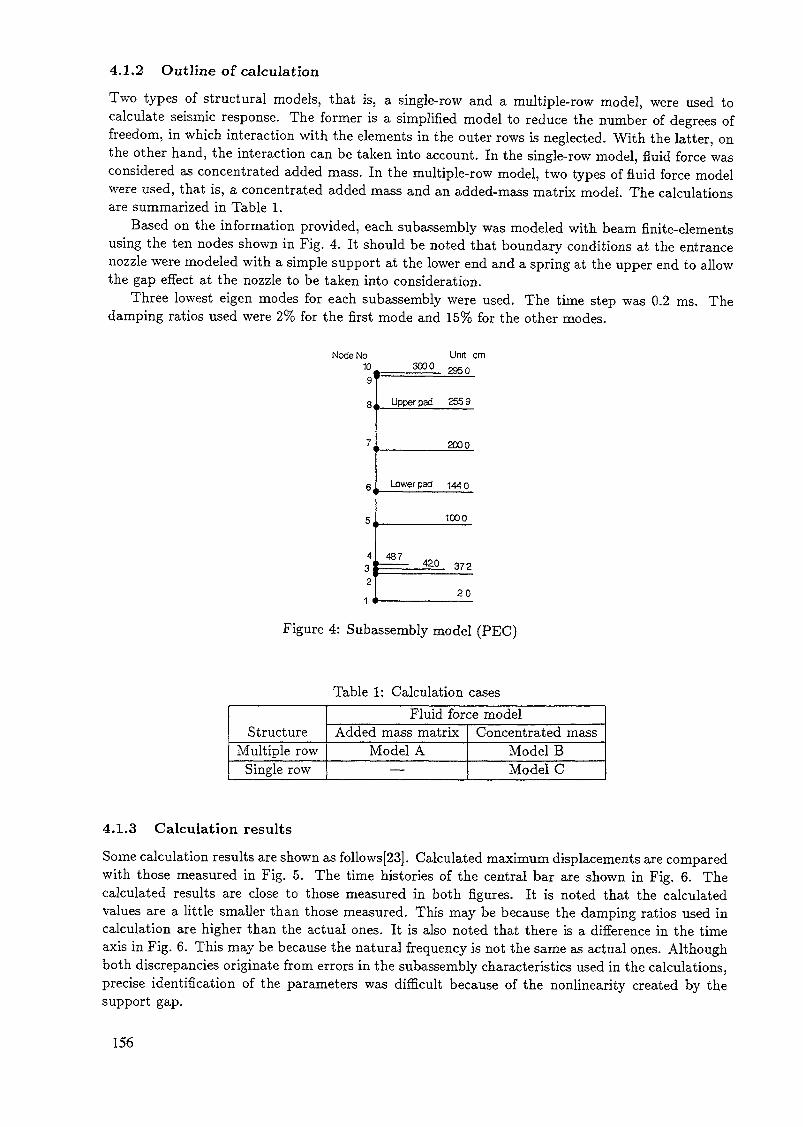
4.1.2 Outline of calculation

Two types of structural models, that is, a single-row and a multiple-row model, were used tocalculate seismic response. The former is a simplified model to reduce the number of degrees offreedom, in which interaction with the elements in the outer rows is neglected. With the latter, onthe other hand, the interaction can be taken into account. In the single-row model, fluid force wasconsidered as concentrated added mass. In the multiple-row model, two types of fluid force modelwere used, that is, a concentrated added mass and an added-mass matrix model. The calculationsare summarized in Table 1.

Based on the information provided, each subassembly was modeled with beam finite-elementsusing the ten nodes shown in Fig. 4. It should be noted that boundary conditions at the entrancenozzle were modeled with a simple support at the lower end and a spring at the upper end to allowthe gap effect at the nozzle to be taken into consideration.

Three lowest eigen modes for each subassembly were used. The time step was 0.2 ms. Thedamping ratios used were 2% for the first mode and 15% for the other modes.

Node No109

8|, Upper pad 2559

321 *

3000Unit cm2950

2000

g Lower pad 144 p

1000

487372

20

Figure 4: Subassembly model (PEC)

Table 1: Calculation cases

StructureMultiple row

Single row

Fluid force modelAdded mass matrix

Model A—

Concentrated massModel BModel C

4.1.3 Calculation results

Some calculation results are shown as follows[23]. Calculated maximum displacements are comparedwith those measured in Fig. 5. The time histories of the central bar are shown in Fig. 6. Thecalculated results are close to those measured in both figures. It is noted that the calculatedvalues are a little smaller than those measured. This may be because the damping ratios used incalculation are higher than the actual ones. It is also noted that there is a difference in the timeaxis in Fig. 6. This may be because the natural frequency is not the same as actual ones. Althoughboth discrepancies originate from errors in the subassembly characteristics used in the calculations,precise identification of the parameters was difficult because of the nonlinearity created by thesupport gap.

156

MeasuredSingle rowMultiple, ConcentratedMultiple, Matrix

B1 A1 AD M B7Bernent

Figure 5: Maximum displacement at top (PEC)

IU

ET 5_o."c<DE 00)Ü05Q.

5-5

•in

i i i i i i--

——— Experiment——— Calculation

/i «—

- * ,1_ i« £ 'A rA I

rv\ A /If HIV *7 jV m

~ \ > iI»

j.

\f r. [l (1 ,H /A A i i A ' 1 1 n / 'A|| Vn/^W1 \ ' ^ \ l ( ' j j |l \l v

1 if i| VM

— J » H

: 'Model A

• i i i i i i

-

--—

:—

*^T-~*"

_

-

10

^o.cQ)E 0(DO

_CÖQ.

5 -5

10

E 5

E 0<DO

_COQ.COQ -5

-10

U 0 1 2 3 4 5 6 7Time (s)

1 1 1 I l

Experiment•Calculation

U0 1 2 3 4Time (s)

ModelB Ij____i5 6 7

• Experiment- Calculation

ModelC -L

0 1 2 3 4 5 6 7Time (s)

Figure 6: Displacement time history of central element (PEC)

157

4.1.4 Discussions

As discussed above, vibration characteristics are nonlinear because of the support gap. This in-fluences not only natural frequency but also damping ratio. Therefore, calculation results largelydepend on how values are determined. Since these nonlinear characteristics are problematic in FBRcore structures to a certain extent, methods to treat nonlinearity should be established.

4.2 Analysis of RAPSODIE experiments

4.2.1 Description of experiments and problems

In the RAPSODIE experiments, 271 subassembly models, including 91 fuel assemblies (the centerand 5 rings) and 180 neutron shield elements (4 rings) were arranged as shown in Fig. 7 andexcited on a shaking table using the earthquake acceleration shown in Fig. 8 [2]. The experimentswere conducted in both air and water. The problem proposed was the calculation of displacementresponse in selected elements. To reduce calculation time, truncated acceleration records were used

Direction of excitation

W 10 " w w "r "g r w w w „ „ ,r

t tf -\f ir nr ir

i- •t-' -vf •>/• ic w -T t

ir -.r w -,/ -,

- "• - w -

V '"' If ?f ""*•?(' *"*•>

v- -Tr' O •î'r v-

~ w " ,-v * w '" v Neutron shieldFuel assembly

RowSRow 7 ;

Row6 (1}'2"3'']4.RowS ' J " "

Row 4 ' n' ]' ]'Row 3

Row 2 ' "Row 1 ' 1 " 2 " 3 ;\ 4 15

1 2 3 " 4 5 6 7 8 9 10 11 12 13 14 15 16 17 18Impact point number

Figure 7: Configuration of subassemblies (RAPSODIE)

10

§-105 10

Time (s)15

(a) Acceleration for in-air experiment

(b) Acceleration for in-water experiment

Figure 8: Time history of input acceleration (RAPSODIE)

158

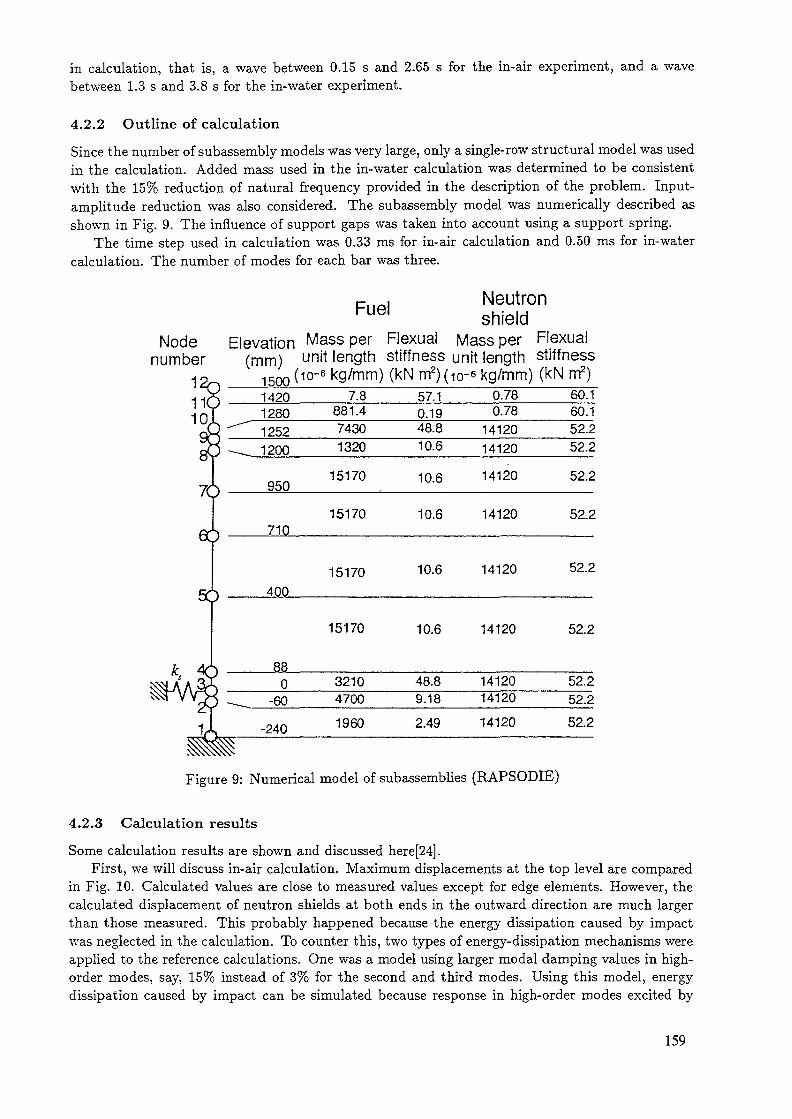
in calculation, that is, a wave between 0.15 s and 2.65 s for the in-air experiment, and a wavebetween 1.3 s and 3.8 s for the in-water experiment.

4.2.2 Outline of calculation

Since the number of subassembly models was very large, only a single-row structural model was usedin the calculation. Added mass used in the in-water calculation was determined to be consistentwith the 15% reduction of natural frequency provided in the description of the problem. Input-amplitude reduction was also considered. The subassembly model was numerically described asshown in Fig. 9. The influence of support gaps was taken into account using a support spring.

The time step used in calculation was 0.33 ms for in-air calculation and 0.50 ms for in-watercalculation. The number of modes for each bar was three.

FuelNode

number1

Neutronshield

Elevation Mass Per F|exual y\ass per Flexual(mm) unit length stiffness unit length stiffness

1500(io-6 kg/mm) (kN m2)(io-6 kg/mm) (kN nf)^1C0t7C

6C

5C

4;1•d

< 1420£ 12803 """' 1252J - 1200

) 950

) 710

) 400

) 88) 0} — _ -60, -240

7.8881.474301320

15170

15170

15170

15170

321047001960

57.10.1948.810.6

10.6

10.6

10.6

10.6

48.89.182.49

0.780.78

141201412014120

14120

14120

14120

141201412014120

60.160.152.252.252.2

52.2

52.2

52.2

52.252.252.2

Figure 9: Numerical model of subassemblies (RAPSODIE)

4.2.3 Calculation results

Some calculation results are shown and discussed here[24].First, we will discuss in-air calculation. Maximum displacements at the top level are compared

in Fig. 10. Calculated values are close to measured values except for edge elements. However, thecalculated displacement of neutron shields at both ends in the outward direction are much largerthan those measured. This probably happened because the energy dissipation caused by impactwas neglected in the calculation. To counter this, two types of energy-dissipation mechanisms wereapplied to the reference calculations. One was a model using larger modal damping values in high-order modes, say, 15% instead of 3% for the second and third modes. Using this model, energydissipation caused by impact can be simulated because response in high-order modes excited by

159

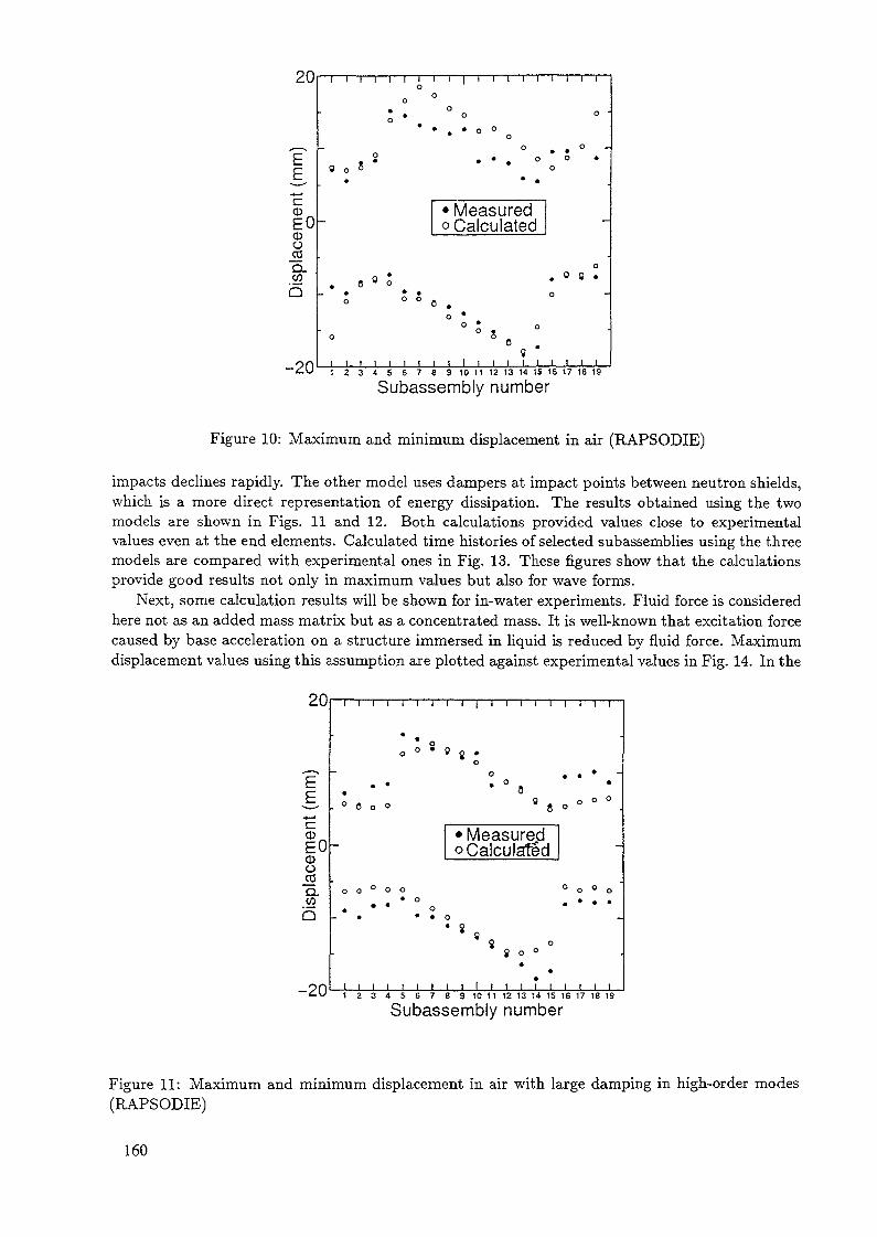
<L\}

acem

ent (

mm

)CLCO

b

-20

— i — i — i — i — i — i — i — i — i — | — i — : — i — \ — i — i i — i — r-O

0 °

* • ° o ° '

8 . • . o * S .9 o * °

• Measuredo Calculated

o

o ° 0 .o •

r ° : s'1 !.. 1 1 1 1 I 1 1 1 1 1 1 1 1 1 1 t 11 a 3 4 S 6 7 3 9 10 11 12 13 14 IS 16 17 18 19

Subassembly number

Figure 10: Maximum and minimum displacement in air (RAPSODIE)

impacts declines rapidly. The other model uses dampers at impact points between neutron shields,which is a more direct representation of energy dissipation. The results obtained using the twomodels are shown in Figs. 11 and 12. Both calculations provided values close to experimentalvalues even at the end elements. Calculated time histories of selected subassemblies using the threemodels are compared with experimental ones in Fig. 13. These figures show that the calculationsprovide good results not only in maximum values but also for wave forms.

Next, some calculation results will be shown for in-water experiments. Fluid force is consideredhere not as an added mass matrix but as a concentrated mass. It is well-known that excitation forcecaused by base acceleration on a structure immersed in liquid is reduced by fluid force. Maximumdisplacement values using this assumption are plotted against experimental values in Fig. 14. In the

20

»pla

cem

ent (

mm

)o

vs

b

-20

I I i 1 1 1 t 1 1 | i ! 1 1 1 | | 1 |

' • oo ° * 0 0 •

oo . . • -

• * * 8 ". * 0 o o « 8 o o ° ° .

• Measuredo Calculated

o o ° o o ° o ° o

« * * o *• • « o -

8 $ °8 o o

**

I i i i i i i t i 1 i i i r i i i i i1 2 3 4 5 6 7 8 9 10 1 1 12 13 14 15 16 17 18 19

Subassembly number

Figure 11: Maximum and minimum displacement in air with large damping in high-order modes(RAPSODIE)

160

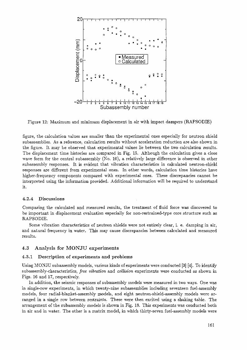
cCDEOCDO03D.W

b

-20

t l i i i

0 o

• Measuredo Calculated

1 1 1 1 1 1 1 t 1 1 1 1 1 1 1 1 1 1l Z 3 4 S 6 7 8 9 10 11 12 13 14 15 16 17 18 19

Subassembly number

Figure 12: Maximum and minimum displacement in air with impact dampers (RAPSODIE)

figure, the calculation values are smaller than the experimental ones especially for neutron shieldsubassemblies. As a reference, calculation results without acceleration reduction are also shown inthe figure. It may be observed that experimental values lie between the two calculation results.The displacement time histories are compared in Fig. 15. Although the calculation gives a closewave form for the central subassembly (No. 10), a relatively large difference is observed in othersubassembly responses. It is evident that vibration characteristics in calculated neutron-shieldresponses are different from experimental ones. In other words, calculation time histories havehigher-frequency components compared with experimental ones. These discrepancies cannot beinterpreted using the information provided. Additional information will be required to understandit.

4.2.4 Discussions

Comparing the calculated and measured results, the treatment of fluid force was discovered tobe important in displacement evaluation especially for non-restrained-type core structure such asRAPSODIE.

Some vibration characteristics of neutron shields were not entirely clear, i. e. damping in air,and natural frequency in water. This may cause discrepancies between calculated and measuredresults.

4.3 Analysis for MONJU experiments

4.3.1 Description of experiments and problems

Using MONJU subassembly models, various kinds of experiments were conducted [3] [4]. To identifysubassembly-characteristics, free vibration and collision experiments were conducted as shown inFigs. 16 and 17, respectively.

In addition, the seismic responses of subassembly models were measured in two ways. One wasin single-row experiments, in which twenty-nine subassemblies including seventeen fuel-assemblymodels, four radial-blanket-assembly models, and eight neutron-shield-assembly models were ar-ranged in a single row between restraints. These were then excited using a shaking table. Thearrangement of the subassembly models is shown in Fig. 18. This experiments was conducted bothin air and in water. The other is a matrix model, in which thirty-seven fuel-assembly models were

161

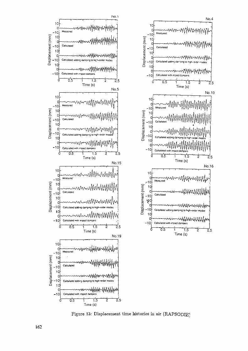
NO. 1No.4

Time (s)No.5

Q._10I. ' "v " "VI<2 Calculated adding damping to high-order modesQ 10

0-1 n ' ' ' '— ' u Calculated with impact dampers

0 0.5 1 1.5Time (s)

2.5

No.15

Measured

101-0;

_-io:E 10£ o"c H n l- Calojiatedo "~ l u

I 108 oS" -10 Calculated adding damping to high-order modes

Q 10o-

— 10 Calculated with impact dampers

0 0.5 1 1.5Time (s)

2.5

No.19—i——•——i——'——i——'——r-

i—~—vvv\ji/*v\jijyy^^Measured I11 ' ' ' "

10|-0

_-10E 10ä o1-10I 10§• — 1 0 f Calculated adding damping to high-order modes

100

— 1 0 \ Calculated with impact dampers

0.5 1 1.5 2Time (s)

2.5

2 25Time (s)

Figure 13: Displacement time histories in air (RAPSODIE'1

162

ö

^_^~J7_i£"""TGoo

•*— 1o<ÜA0.4E

«•— •

E13l^_

— 2Xe-CÖ^>

0

i i i i i i t

o TopD Top

D • Pad. Pad

D ' ———————

D

D

D

—D

0 O

~~ O °0 0

0

" • i :1 1 1 1 1 1 11 2 3 4 5 6 7

i i 1 i i t i i i i ta

with participation factorwithout participation factor Qwith participation factorwithout participation factor

D

oa o _

aa0a a a

D ° ?« ° °0 °o -

,;,..':1 1 1,... 1 1 1 1 i 1 1 i8 9 1011 12131415161718

Impact point numberFigure 14: Maximum and minimum displacement1 in water (RAPSODIE)

hexagonally arranged in a restraint ring and excited using a shaking table in air and in water. Theschematic of the 37-bar matrix experiments is shown in Fig.19.

Input-acceleration time history is shown in Fig. 20. The time history was scaled down toseveral amplitudes for the experiment. The seismic-response calculations were conducted using thea history record from 9 s to 14 s to reduce calculation time.

4.3.2 Outline of calculation

Calculations were conducted corresponding to experiments for subassembly-characteristic identi-fication using a fine finite-element model with 50 nodes, which is able to accommdate high-ordereigen modes (up to 48th) induced by impact force.

Seismic responses were calculated using the simplified numerical model as shown in Fig. 21. Itshould be noted that the effect of the gap at the support was considered by also using a springat the support in this model. It should additionally be noted that stiffness at the load pad wasmodified to a value at which the calculated impact force for the collision was close to the measuredone. For matrix experiments, the structure was assumed using a single-row or multiple-row model.The fluid force was modeled using an added-mass matrix or a concentrated added mass. Thecalculation cases are the same as for the PEC experiments, as summarized in Table 1.

4.3.3 Calculation results

Some calculation results follows [25]. Impact forces corresponding to collision experiments werecalculated as shown in Figs. 22 and 23. Figure 22 shows force at the middle load pad. In thefigure, the calculated results agree the experimental ones not only in maximum values but also intime history pattern, that is, there are two peaks for an impact. Figure 23 is the force at the topload pad, in which the calculated maximum force is larger than the measured force although themaximums of impact forces occur almost at the same time. This may be because a phenomenonwhich is unable to be considered using the present beam model (e. g. deflection in plane) occurredduring the actual impact. For seismic-response calculation, stiffness at a load pad was modifiedto be a value at which the calculated impact force for the collision experiment was close to themeasured one.

163

No. 1

_£_-'Cj- Measured

- id-

Q. iq-tnQ

-icf

Calculated with participation factor

Calculated witnqut participation lactor ,0 0.5 1 1.5

Time (s)2 2.5

cOJ

S-.ctJOQ.Wb o[

No. 4

— '-•"'••-•'••'"•-vWV-"1^Calculated with participation laclor

Calculaied without participai'on factor

0 0.5 1 1.5Time (s)

2 2.5

No. 5 No. 10

Disp

lace

men

t (m

m

Calculated with participation lactor

Calculated without participation lactor

0 0.5 1 1.5 2 2.5Time (s)

1 1.5Time (s)

No. 15

U

CD

h"O. 1Ctob "

-1C

\ —— ' —— i

Calculated with participation (actor

0 0.5 <d.oTime (s)

No-16

E-1CJ- Measured

¥ «*-a>OJu-11jgQ.to

Calculated with participation factor

-icf- Calculaied wilhout participation lactor

Time(s)v '

No. 19

i-c 1C<

i *

3-1•Q. iqto

Measured

Calculated with participation factor

[—•——^^^^fA/^fVl|W^^.Caicyîated wiihqm participation (actor,

0 0.5 1 1.5 2 2.5Time (s)

Figure 15: Displacement time histories in water (RAPSODIE)

164

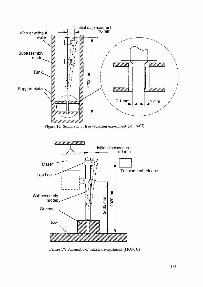
With or withoutwater

Subassemblymodel

Tank,

Support plate

1

r

'

/"is/v/////

-] i-,r/•** *»»rtvr

ift' r"V

1 t *4ft

t 4

f

'-N

Initial dis

i4t1

\s/S/SS/f.

}s/s////r/.

'/////////////////A

//11 1

EEooCM

1

pla

i

^

r

10 mm

w/////////.

V//////////<

0.1 mm^ ^^ ^— -

'//////////A

W///////A

0.1 mm— -

Figure 16: Schematic of free vibration experiment (MONJU)

W//////////S////////A

Subassemblymode!

Initial displacement50 mm

Tension and release

Figure 17: Schematic of collision experiment (MONJU)

165

Bar number1 2 3 4 5 6 7 8 91011121314151617181920212223242526272829

OOOOOOOOOOÛOOÛÛOOOOOOOOOOOOOE1 2 3 4 5 6 7 8 9101112131415161718192021222324252627282930

Impact force^*

.Displacement

Position ofstrain measurement

x Strain

Fuel assmbly model

Blancket assembly model

"Neutron shieldmodel

Figure 18: Schematic of single-row 29-subassembly experiment (MONJU)

Tank

Impact force ',

Figure 19: Schmatic of 37-bar matrix experiments (MONJU)

166

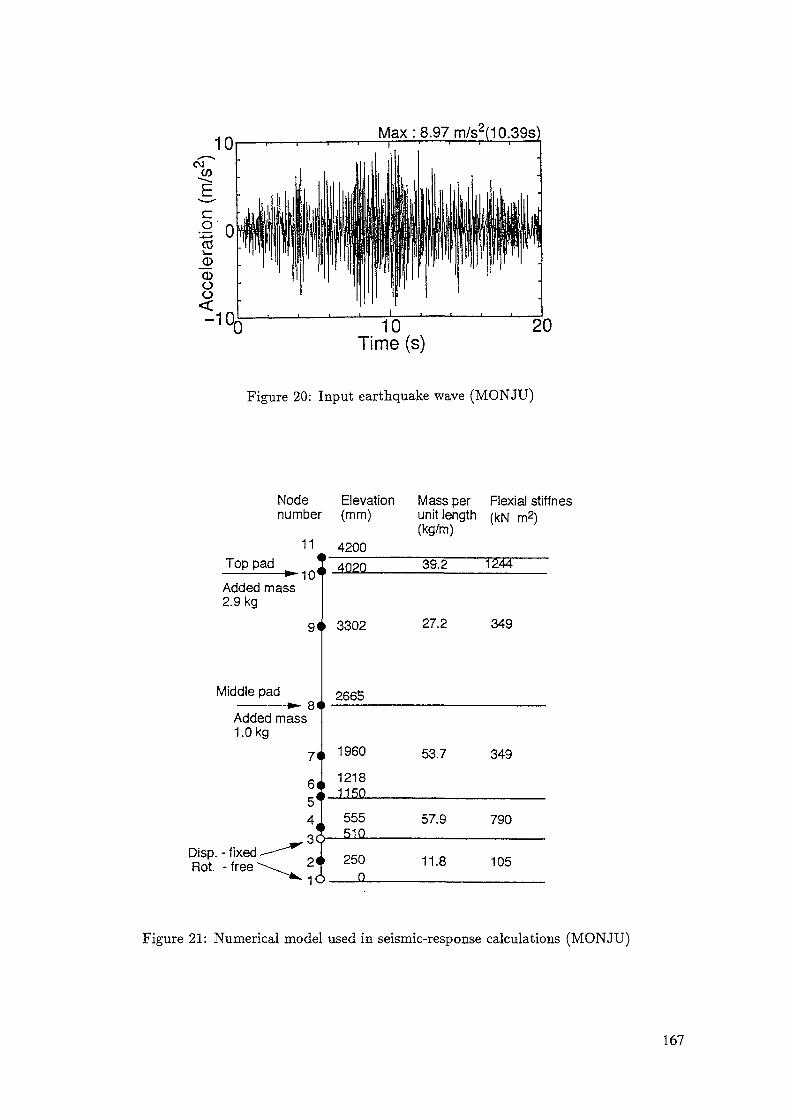
t)

Max: 8.97 m/s2(10.39s)

10Time (s)

20

Figure 20: Input earthquake wave (MONJU)

Node Elevation Mass per Flexial stiff n esnumber (mm) unit length (kN m2)

(kg/m)4200

DispRot.

Top pad

Added mass2.9kg

Middle pad———— f,Added mas1.0kg

-fixed— -^^- free '~^\_^

10*

9«

- 8«s

7<

6«5*4

.3C

2<- 1C

t 4020

i 3302

2665i ——————

, 1960

1218! 1150

555I 510

» 250\ 0

39.2 1244

27.2 349

53.7 349

57.9 790

11.8 105

Figure 21: Numerical model used in seismic-response calculations (MONJU)

167

Table 1: Calculation cases

StructureMultiple row

Single row

Fluid force modelAdded mass matrix

Model A—

Concentrated massModel BModel C

0 10Time (ms)

20

Figure 22: Calculation results for impact force at middle load pad (MONJU)

100Calculated

Measured

2 3 4 5Time (ms)

Figure 23: Calculation results for impact force at top load pad (MONJU)

168

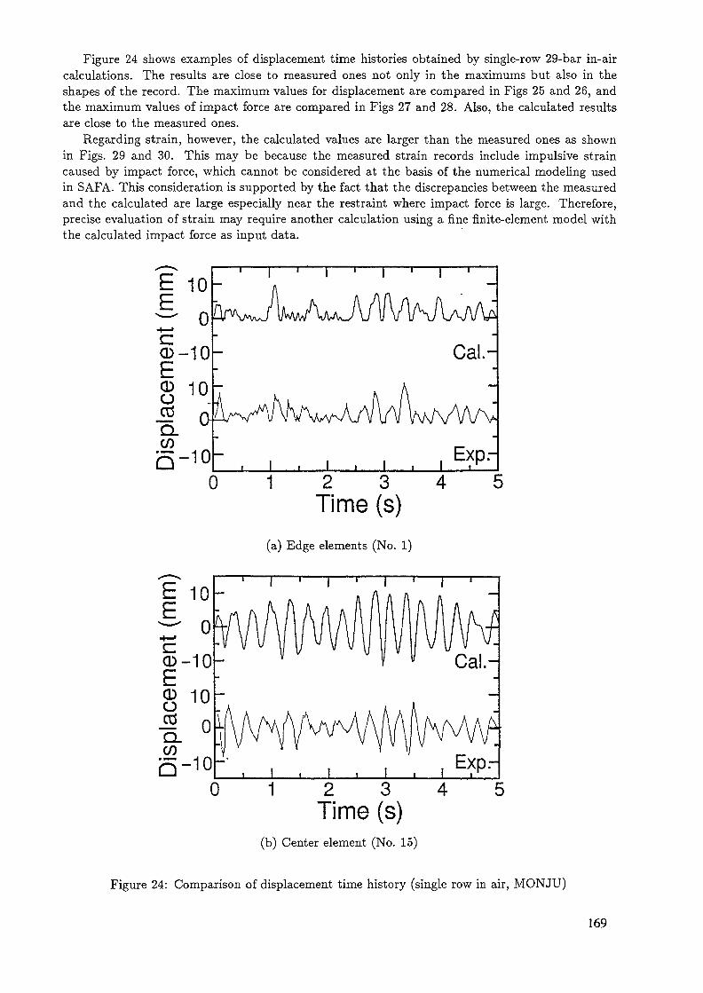
Figure 24 shows examples of displacement time histories obtained by single-row 29-bar in-aircalculations. The results are close to measured ones not only in the maximums but also in theshapes of the record. The maximum values for displacement are compared in Figs 25 and 26, andthe maximum values of impact force are compared in Figs 27 and 28. Also, the calculated resultsare close to the measured ones.

Regarding strain, however, the calculated values are larger than the measured ones as shownin Figs. 29 and 30. This may be because the measured strain records include impulsive straincaused by impact force, which cannot be considered at the basis of the numerical modeling usedin SAFA. This consideration is supported by the fact that the discrepancies between the measuredand the calculated are large especially near the restraint where impact force is large. Therefore,precise evaluation of strain may require another calculation using a fine finite-element model withthe calculated impact force as input data.

E 10'•— o-t—»

§5-10g 10! oMQ-10

E 10^- o•4— '

§5-10

8 1003"o.CO5-10

nu

I ' i I '

Cal.-

Exp.-0 1 2 3

Time (s)(a) Edge elements (No. 1)

Exp.-0 1 2 3 4 5

Time (s)(b) Center element (No. 15)

Figure 24: Comparison of displacement time history (single row in air, MONJU)

169

15

••—•>

§10

CD

CD

46COb

0

I 1 I I I I I ! 1 I I I i I 1 I I I ( I I I i | l ) | i i

(1 G = 9.806 m/s2)

0.1 G (Cal.),

0.1 G (Exp.)

i i i i i i i i i l i i i i i i i i i l i i i i i i i i i15

Bar number29

Figure 25: Maximum displacement (single row in air, MONJU)

15

I10•*-«CD

CDÜCOQ. 5COb

0

(1 G = 9.806 m/s"1)

Center (Cal.)

/,* Edge(Exp.)/

'' p Center (Exp.)Edge (Cal.)

0.2 0.4Input acceleration (G)

Figure 26: Maximum displacements for different maximum input accelerations (single row in air,MONJU)

170

20

CDüo10

crjQ.

0

"i i i i i i i n i i n i i i i i i | i i i i i IT n rTop pad

.0.3 G (Exp.) rr

0.3 G (Exp.)

f0.1 G (Exp.) -

i i i i i i t l i i i i i i t i i l i i i i i i i i i I

Impact point number 30

Figure 27: Maximum force (single row in air, MONJU)

20 _ (1 G = 9.806 m/s2

03Ü .

üCOQ.

o

Top padNo.1 (Cal.)

No.1 (Exp.)

No.30 (Exp.)

No.30 (Gal.)

Middle pad.No.1 (Cal.)

o.30 (Cal.)No.1 (Exp.)No.30 (Exp.) _

0 0.2 0.4Input acceleration (G)

Figure 28: Maximum forces for different maximum input accelerations (single row in air, MONJU)

171

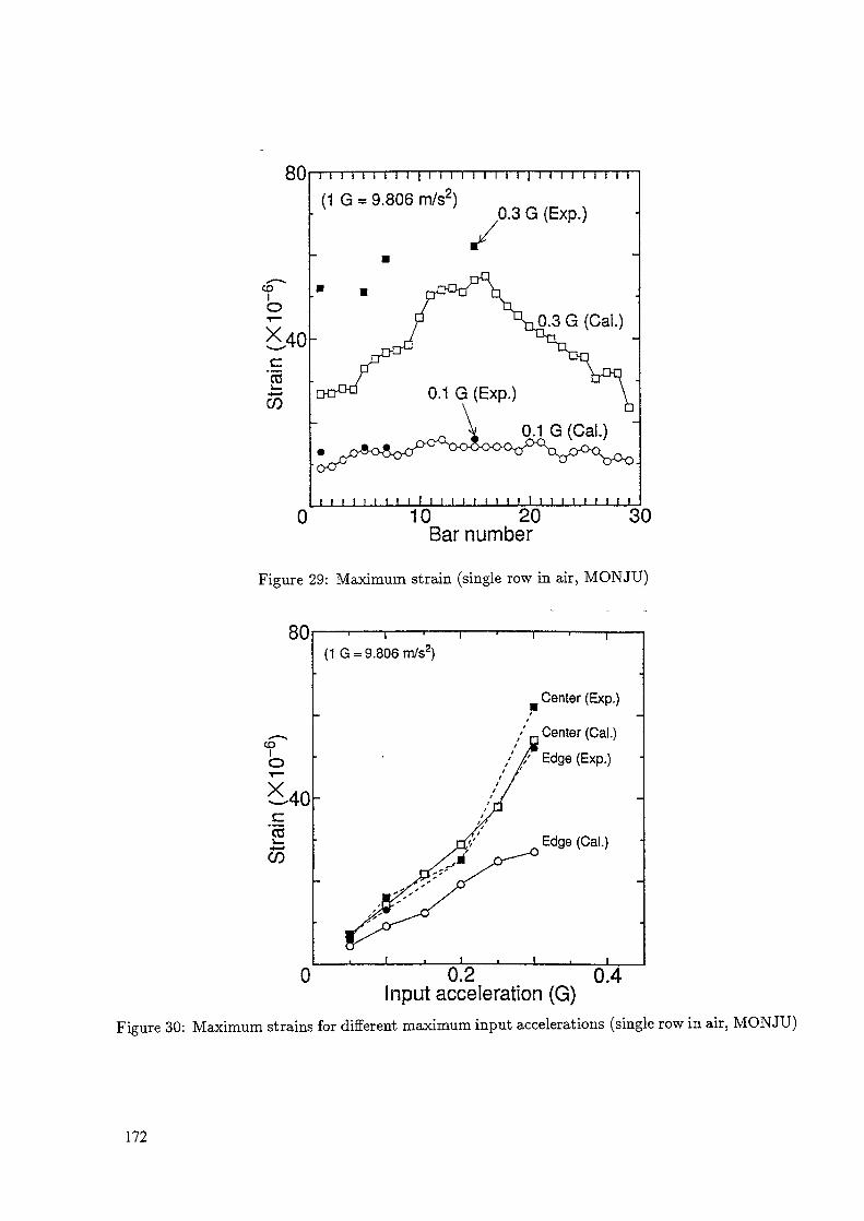
80

COI

><40c

"co•<—»CO

(1 G = 9.806 m/s2).0.3 G (Exp.)

.3 G (Cal.)

0 10 20Bar number

30

Figure 29: Maximum strain (single row in air, MONJU)

80

coO

X 40

co

(1 G = 9.806 m/s2)

Center (Exp.)/

/ o Center (Cal.)

/ / Edge (Exp.)

Edge (Cal.)

0 0.2 0.4Input acceleration (G)

Figure 30: Maximum strains for différent maximum input accelerations (single row in air, MONJU)

172

As examples of results obtained from 37-bar matrix calculations, the maximum impact force inthe in-water experiments are shown in Figs. 31 and 32.

The followings can be established from a comparison with the calculated results. With concen-trated mass models (B, C), the impact forces from the single-row model (C) were larger than thosefrom the multiple-row model (B). This may be due to the following reasons. In the experiment,impact between subassembly models in different rows took place and the energy in the exciteddirection was dissipated. Since the single-row model is unable to account for this effect, the impactforces increased. With multiple-row models (A, B), impact forces from the concentrated addedmass (B) were larger than those from the added mass matrix model (A). This can be understoodas follows: The fluid-structure interaction considered in Model A makes subassembly models vi-brate in phase and thus reduces interaction by impact between subassembly models in differentrows. Therefore, energy dissipation in the excitation direction becomes small.

20

1 0

CLE

i——r n——r i——r i——r

0.5 GCal. (Model C)

- Cal. (Model

Cal. (Model ACal. (Model B/

(1 G = 9.806 m/sTop pad

t___I___I 1___I___I___I___I

1 8impact point numberFigure 31: Maximum force (matrix in water, MONJU)

o- ^fe

MiddleCal. (Model A) •

/Cal. (Model C)

Exp.

Cal. (Mode! BX_

0.2 0.4 0.6 0.8Input acceleration (G)

Figure 32: Maximum forces for different maximum input accelerations (matrix in water, MONJU)

173

In a comparison between calculated results and measured ones, measured values are relativelysmaller than those calculated using Model A although it is the most precise model of the three.This can be understood in the following way. In the calculation, impact between the edge elementin the central row and the restraint occurs only in the direction of excitation because the half-plane model is used. In the experiment, however, impact in a different direction occurred as shownin Fig. 33. This means that the motion of the subassembly model was restrained in two or threedirections. Therefore, impact force became smaller than the perfect symmetrical motion consideredin the calculation.

0.3 G (2.94 m/s2) excitaion

6.0 kN 4.6 kN

OkN 3.9 kN

(a) Calculated(Model A)

(b) Measured(37 bars, in water)

Figure 33: Maximum impact force for impact direction (MONJU)

4.3.4 Discussions

In restrained-type core structures such as MONJU, it is obvious that impact force is an importantresponse value. As observed in the above discussions, proper impact parameters are necessary toobtain accurate predictions of impact force by calculation. Therefore, experiments to determinevalues are essential for seismic response analysis in actual core structures.

From calculations of matrix experiments, impact phenomena between subassemblies in differentrows were found to be significant in impact force evaluation. In addition, motion in directionsother than that of excitation is also important in some cases. The single-row model is unable toaccomodate such phenomenon, but it is useful as a simplified method to obtain approximate results.

5 Comparison of solutions

5.1 Comparison of programs

Some features of the computer programs used in this benchmark-analysis CRP are shown in Table 2.The programs are divided roughly into two types. One is for those using the direct integrationmethod, the other is for those using the modal superposition method. The numerical structuralmodels are almost identical. Various time integration algorithms were utilized.

In the following sections, solutions obtained by the varios programs will be compared. However,comparisons will be limited on MONJU single-subassembly experiments and PEC experiments

Table 2: The computer programs participating in the benchmark analysis

NameOrganization

PurposeCalcualuon method*

Tune integrationElement modelImpact model

SAFAHitachi,JapanSpecficModalNigainBeam

Gap+Spring

CASTEMCEA,FranceGeneralDirect

—Beam

Gap+Spnng

CORE-SEISIGCAR,

IndiaSpecificDirect

Newmark-^Beam

Gap+Spring

COSMOSBAEC,India

SpecificModel

Newmark-/?Beam

Gap+Spnng

DINAEAOKBM,RussiaGeneralDirect

Central differenceBeam

Gap+Spring

FINASPNC,Japan

GeneralDirect

Newmark-,9Beam

Gap+Spring

FINDSMffl,Japan

SpecificModal

Modified Tailor developmentBeam

Gap+Spring

SALOONToshiba,Japan.

SpecificDirect

Hubert-HughBeam

Gap+Spring« Modal — Modal superposition, Direct — Direct integration

174

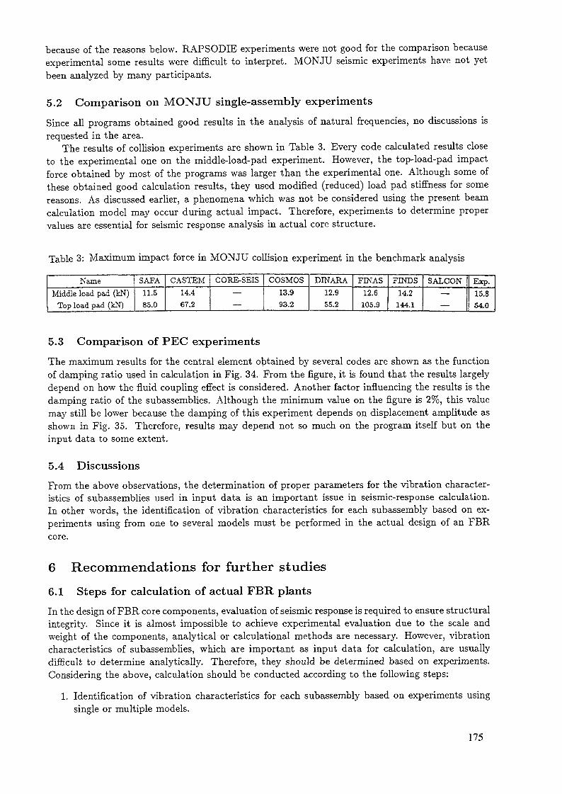
because of the reasons below. RAPSODIE experiments were not good for the comparison becauseexperimental some results were difficult to interpret. MONJU seismic experiments have not yetbeen analyzed by many participants.

5.2 Comparison on MONJU single-assembly experiments

Since all programs obtained good results in the analysis of natural frequencies, no discussions isrequested in the area.

The results of collision experiments are shown in Table 3. Every code calculated results closeto the experimental one on the middle-load-pad experiment. However, the top-load-pad impactforce obtained by most of the programs was larger than the experimental one. Although some ofthese obtained good calculation results, they used modified (reduced) load pad stiffness for somereasons. As discussed earlier, a phenomena which was not be considered using the present beamcalculation model may occur during actual impact. Therefore, experiments to determine propervalues are essential for seismic response analysis in actual core structure.

Table 3: Maximum impact force in MONJU collision experiment in the benchmark analysis

NameMiddle load pad (kN)

Top load pad (kN)

SAFA11.585.0

CASTEM14.467.2

COKE-SEIS

I

COSMOS13.993.2

DIN ARA12.955.2

FINAS12.6105.9

FINDS14.2144.1

SALCON• ——

Exp.15.854.0

5.3 Comparison of PEC experiments

The maximum results for the central element obtained by several codes are shown as the functionof damping ratio used in calculation in Fig. 34. From the figure, it is found that the results largelydepend on how the fluid coupling effect is considered. Another factor influencing the results is thedamping ratio of the subassemblies. Although the minimum value on the figure is 2%, this valuemay still be lower because the damping of this experiment depends on displacement amplitude asshown in Fig. 35. Therefore, results may depend not so much on the program itself but on theinput data to some extent.

5.4 DiscussionsFrom the above observations, the determination of proper parameters for the vibration character-istics of subassemblies used in input data is an important issue in seismic-response calculation.In other words, the identification of vibration characteristics for each subassembly based on ex-periments using from one to several models must be performed in the actual design of an FBRcore.

6 Recommendations for further studies

6.1 Steps for calculation of actual FBR plantsIn the design of FBR core components, evaluation of seismic response is required to ensure structuralintegrity. Since it is almost impossible to achieve experimental evaluation due to the scale andweight of the components, analytical or calculational methods are necessary. However, vibrationcharacteristics of subassemblies, which are important as input data for calculation, are usuallydifficult to determine analytically. Therefore, they should be determined based on experiments.Considering the above, calculation should be conducted according to the following steps:

1. Identification of vibration characteristics for each subassembly based on experiments usingsingle or multiple models.

175

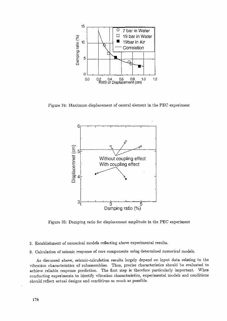
£o 10"5O)

1 5öSQ

0

0

\\\

° 7 bar in Water° 19 bar in Water• IQbarinAir

— Correlation

m'X,

*E -B-

0 0.2 0.4 0.6 0.8 1.0 1.R MS of Displacement (cm)

Figure 34: Maximum displacement of central element in the PEC experiment

IsECDÜ

_TO

g-4b

Without coupling effectWith coupling effect

3 5Damping ratio (%)

Figure 35: Damping ratio for displacement amplitude in the PEC experiment

2. Establishment of numerical models reflecting above experimental results.

3. Calculation of seismic response of core components using determined numerical models.

As discussed above, seismic-calculation results largely depend on input data relating to thevibration characteristics of subassemblies. Thus, precise characteristics should be evaluated toachieve reliable response prediction. The first step is therefore particularly important. Whenconducting experiments to identify vibration characteristics, experimental models and conditionsshould reflect actual designs and conditions as much as possible.

176

6.2 Criterion for seismic integrity of FBR cores

Needless to say, seismic integrity is an important design factor for FBR' core components. Integritydepends on vibration responses of subassemblies, such as displacement, impact force and strain.Therefore the programs used for the benchmark analysis were made to output such response values.Although it is difficult to define clear criteria for integrity, it is necessary to define some criteriaand to clarify requirements for programs, to develop further improved calculation programs in thefuture.

7 Conclusions

As a project of IAEA/IWGFR, a coordinated research program on intercomparison of LMFBRseismic analysis codes has been performed since 1991. During this research program, the partic-ipants have conducted calculations on PEC, MONJU and RAPSODIE problems using their owncomputer programs.

This report reviewed the results calculated using the SAFA program developed by Hitachi, Ltd.In all problems, the calculated results using SAFA were close to measured values within a certaindegree of accuracy. Therefore, it can be concluded that SAFA has the capability to be used inseismic-response analysis of FBR cores for practical use. However, some research on fluid force oradded mass may be required to improve results not only for SAFA but also for other codes.

Also the intercomparison of computer codes and recommendations for future research werediscussed. During the discussion, the importance of identification of subassembly vibration char-acteristics was emphasized.

References

[1] Test data, Distributed to participants of IAEA/IWGFR/CRP on intercomparison of LMFBRSeismic Analysis Codes, (1991).

[2] Brochard, D., Proposed Benchmark Problem for IAEA/Coordinated Research Program onInter Comparison of LMFBR Seismic Analysis Codes: Seismic Analysis of Thee FBR CoreMock-up Rapsodie, Distributed to the participants of IAEA/IWGFR/CRP on intercomparisonof LMFBR Seismic Analysis Codes, (1993).

[3] Iwata, K., Nakanishi, S., Morishita, M., Ohtsubo, T. and Inoue, T., Proposed BenchmarkProblems for IAEA/IWGFR Coordinated Research Program on Intercomparison of LMFBRSeismic Analysis Codes, Distributed to the participants of IAEA/IWGFR/CRP, (1991).

[4] Morishita, M., Proposed Benchmark Problems from MONJU Core Mock-up Experiments,Distributed to participants of IAEA/IWGFR/CRP on intercomparison of LMFBR SeismicAnalysis Codes, (1992).

[5] Fujita, K., Vibration characteristics and seismic response of grouped column in liquid, Trans.Jpn. Soc. Mech. Eng., 47-415, C, (1981), 251, (in Japanese).

[6] Preumont, A. et al, Fluid-Coupling Effects in LMFBR Core Seismic Analysis, Proc. 7th Int'lConf. on Struct. Mech. in Reactor TechnoL, E, E6/7, (1983), 275.

[7] Horiuchi, T., and Nakagawa, M., A three-dimensional analysis of added mass for earthquakeresponse of hexagonal bars immersed in liquid, Trans. Jpn. Soc. Mech. Eng. ser. C, 59-557,(1993), 93 (in Japanese).

[8] Horiuchi, T. and Nakagawa, M., Study on the impact vibration of grouped bars by shakingtable experiments, Trans. Jpn. Soc. Mech. Eng. ser. C, 55-512, (1989), 860 (in Japanese).

177

[9] Sasaki, Y. and Muto, T., Experimental Studies on Seismic Vibration Phenomena of FBRCore Components, Proc. 7th Int'l Conf. on Struct. Meek, in Reactor TechnoL, E, F6/7,(1983), 315.

[10] Martelli, A., Forni, M. Masoni, P. Marrsca, G. Castoldi, A. and Muzzi, F., Research andDevelopment Studies on Plant and Core Seismic Behavior for A Fast Reactor, Nucl. Eng.Des., 106, (1988), 103.

[11] Brochard, D., Buland, P., Gantenbein, F. and Gibert, R. J., Seismic Analysis of LMFBRCores, Mock-up RAPSODIE, Proc. 9th Int'l Conf. on Struct. Meek, in Reactor TechnoL, E,(1987), 33.

[12] Preumont, A., Pay, A. and Decauwers, A., The Seismic Analysis of a Free Standing FBRCore, A Case Study — SNR-2 Preliminary Design, Nucl Eng. Des., 103, (1987), 199.

[13] Brochard, D., Hammami, L. and Gantenbein, F., FBR Core Mock-Up Rapsodie II: NumericalModels, Proc. Int'l Conf. on Fast Reactor Core and Fuel Struct. Behavior, (1990), 199.

[14] Morishita, M. and Iwata, K., Seismic Behavior of a Free-Standing Core in a Large LMFBR,Nucl Eng. Des., 140, (1993), 309.

[15] Guyan, R. J., Reduction of Stiffness and Mass Matrix, AIAA J., 3 , (1965), 380.

[16] Sasaki, Y., Manome, E. and Kakehi, I., Seismic analysis of LMFBR core components, Trans,llth Int'l. Conf. Structural Mechanics in Reactor Technology, (1991), E, 491.

[17] Horiuchi, T., Nakagawa, M. and Kasai, H., Development of SAFA, A Seismic Analysis Pro-gram for FBR Core Components, Nucl Eng. Des., (To be published).

[18] Aida, Y., et al., Experimental and Analytical Studies on Vertical Response of FBR CoreComponents during Seismic Events Proc. 12th Int'l Conf. on Struct. Mech. in Reactor TechnoL,E, (1993), 33.

[19] Amada, et al. Study of Reactor Core Seismic Analysis Method, (1) - (4), Proc. Spring Conf.of Japan Atomic Society, F58 - F61, (1993), 346 - 349.

[20] Tomita, H., Flow-Path Network Method Analysis of the Vibration Characteristics of a Groupof Rods in Fluid, Trans. Jpn. Soc. Mech. Eng., 49-445, C, (1983), 1474, (in Japanese).

[21] Shar, V. N., Bohm, G. J. and Nahavandi, A. N., Modal Superposition Method for Computa-tionally Economical Nonlinear Structural Analysis, Trans. ASME, J. Press. Vessel TechnoL,101, (1979), 134.

[22] Nigam, N. C. and Jennings, P. C., Calculation of Response Spectra from Strong MotionEarthquake Records, Butt. Seism. Soc. of Am., 59, (1969), 902. .

[23] Horiuchi, T. and Motomiya, T., Seismic Analysis for PEC Fast Reactor Core Experiments Us-ing The SAFA Program, IAEA/IWGFR/CRP on intercomparison of LMFBR Seismic Anal-ysis Codes, Vienna, Austria, (1993).

[24] Horiuchi, T. and Motomiya, T., Seismic Analysis for the FBR Core Mock-up Rapsodie Experi-ments Using the SAFA Program, IAEA/IWGFR/CRP on intercomparison of LMFBR SeismicAnalysis Codes, O-arai, Japan, (1994).

[25] Horiuchi, T., Seismic Analysis for MONJU Core Seismic Experiments Using the SAFA Pro-gram, IAEA/IWGFR/CRP on intercomparison of LMFBR Seismic Analysis Codes, Bolonga,Italy, (1995).

178

SEISMIC ANALYSIS FOR MONJU CORE SEISMICEXPERIMENTS USING THE SAFA PROGRAM

T. HORIUCHIMechanical Engineering Research Laboratory,Hitachi Ltd,Tsuchiura, Ibaraki,Japan

Abstract

As a part of the IAEA/IWGFR coordinated research program on LMFBR seismic analysiscodes, the results of MONJU core seismic experiments conducted by PNC Japan, were analyzedand the experimental and the calculated results were compared. For these analyses, the com-puter program SAFA was utilized. This program was developed by Hitachi, Ltd., to analyzevibration of fast breeder reactor core components during seismic excitation. In comparisonsof displacements and impact forces, the calculated results were close to the experimental ones.However, on strains, the calculated results were smaller than the measured ones. This maybe because the measured strain records include impulsive strain caused by impact force, whichcannot be taken into account using the numerical model used in SAFA. Since the results werein good agreement in general, the effectiveness of the SAFA can be considered to have beenverified.

1 INTRODUCTIONAs a part of the IAEA/IWGFR coordinated research program on LMFBR seismic analysis codes,problems based on the results of the MONJU core seismic experiments, and which were proposedby PNC Japan [1], were analyzed.

The computer program SAFA (Seismic Analysis program for Fuel Assemblies) was applied.This program was developed by Hitachi, Ltd. to analyze core-component vibration of fast breederreactors (FBR) during seismic excitation.

In this paper, after a short description of the SAFA program, discussions on the calculationmodels will be given in detail. Afterwards the results of seismic analyses based on these modelswill be shown.

2 DESCRIPTION OF THE SAFA PROGRAM

The SAFA program models subassemblies using beam finite-elements and treats impact phenomena,between two subassemblies or between a subassembly and a restraint, using sets of gaps, springsand dampers. A schematic view of the numerical model is shown in Fig. 1.

The program introduces fluid force into the calculation using one of the following two addedmass models. One is a three-dimensional added-mass matrix, with which the interaction betweenthe subassemblies and the core barrel, due to fluid force, can be precisely considered. The otheris a concentrated added mass matrix, which is a simplified method for treating the fluid/structureinteraction, by using which the natural frequency of the first mode of the subassemblies can besimulated.

The program integrates the equation of motion for seismic-response with respect to time, makinguse of mode superposition with the pseudo-external force method [2], in which impact force isdetermined using a newly-developed algorithm that doesn't require multiple convergence iterations[3]. SAFA neglects high-order modes which have little contribution to seismic response, in order toreduce the number of degrees of freedom in calculation. Detailed discussions on the SAFA programare given elsewhere [4, 5],

179

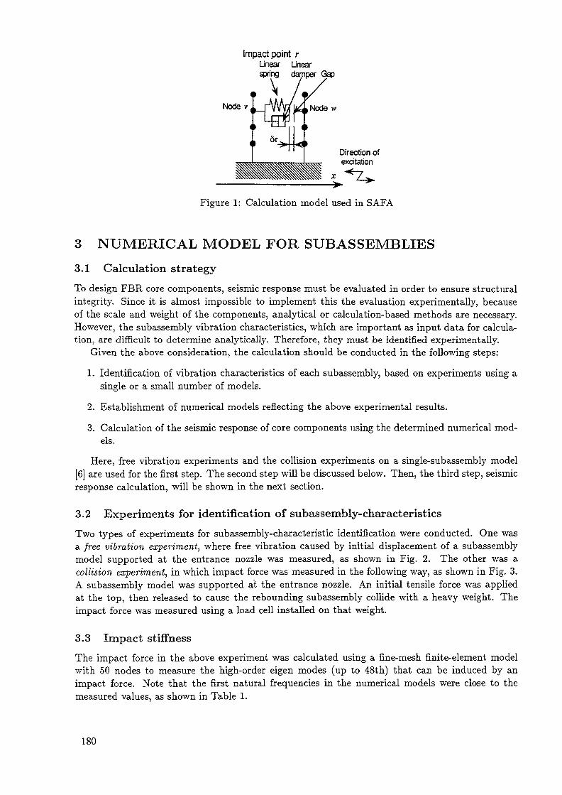
Impact point rLinear Linearspring damper Gap

Node v

Direction ofexcitation

Figure 1: Calculation model used in SAFA

3 NUMERICAL MODEL FOR SUB AS SEMBLIES

3.1 Calculation strategy

To design FBR core components, seismic response must be evaluated in order to ensure structuralintegrity. Since it is almost impossible to implement this the evaluation experimentally, becauseof the scale and weight of the components, analytical or calculation-based methods are necessary.However, the subassembly vibration characteristics, which are important as input data for calcula-tion, are difficult to determine analytically. Therefore, they must be identified experimentally.

Given the above consideration, the calculation should be conducted in the following steps:

1. Identification of vibration characteristics of each subassembly, based on experiments using asingle or a small number of models.

2. Establishment of numerical models reflecting the above experimental results.

3. Calculation of the seismic response of core components using the determined numerical mod-els.

Here, free vibration experiments and the collision experiments on a single-subassembly model[6] are used for the first step. The second step will be discussed below. Then, the third step, seismicresponse calculation, will be shown in the next section.

3.2 Experiments for identification of subassembly-characteristics

Two types of experiments for subassembly-characteristic identification were conducted. One wasa free vibration experiment, where free vibration caused by initial displacement of a subassemblymodel supported at the entrance nozzle was measured, as shown in Fig. 2. The other was acollision experiment, in which impact force was measured in the following way, as shown in Fig. 3.A subassembly model was supported at the entrance nozzle. An initial tensile force was appliedat the top, then released to cause the rebounding subassembly collide with a heavy weight. Theimpact force was measured using a load cell installed on that weight.

3.3 Impact stiffness

The impact force in the above experiment was calculated using a fine-mesh finite-element modelwith 50 nodes to measure the high-order eigen modes (up to 48th) that can be induced by animpact force. Note that the first natural frequencies in the numerical models were close to themeasured values, as shown in Table 1.

180

With or withoutwater

Subassemblymodel

Tank

Support plate

Initial displacement10mm

Figure 2: Schematic of free vibration experiment

Initial displacement50mm

Tension and release

Subassemblymodel

Figure 3: Schematic of collision experiment

181

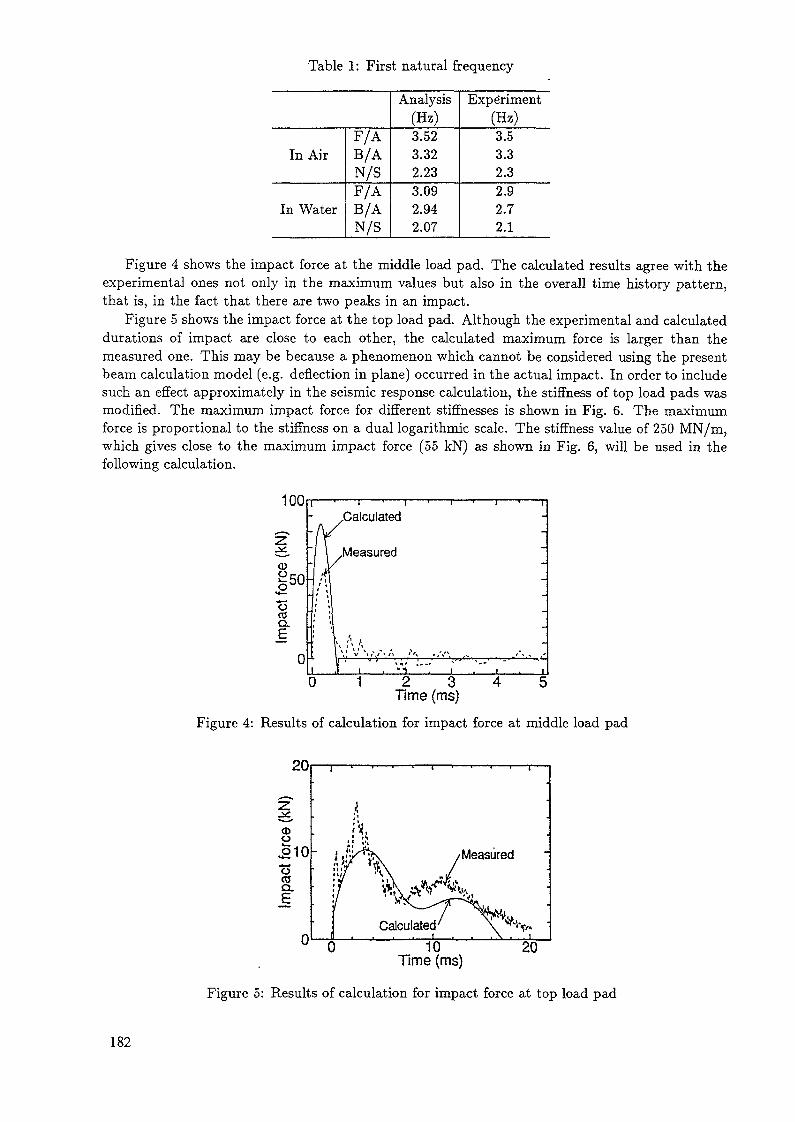
Table 1: First natural frequency

In Air

In Water

F/AB/AN/SF/AB/AN/S

Analysis(Hz)3.523.322.233.092.942.07

Experiment(Hz)3.53.32.32.92.72.1

Figure 4 shows the impact force at the middle load pad. The calculated results agree with theexperimental ones not only in the maximum values but also in the overall time history pattern,that is, in the fact that there are two peaks in an impact.

Figure 5 shows the impact force at the top load pad. Although the experimental and calculateddurations of impact are close to each other, the calculated maximum force is larger than themeasured one. This may be because a phenomenon which cannot be considered using the presentbeam calculation model (e.g. deflection in plane) occurred in the actual impact. In order to includesuch an effect approximately in the seismic response calculation, the stiffness of top load pads wasmodified. The maximum impact force for different stiffnesses is shown in Fig. 6. The maximumforce is proportional to the stiffness on a dual logarithmic scale. The stiffness value of 250 MN/m,which gives close to the maximum impact force (55 kN) as shown in Fig. 6, will be used in thefollowing calculation.

100

CD

Q,

0

.Calculated

Measured

0 1 2 3 4 5Time (ms)

Figure 4: Results of calculation for impact force at middle load pad

20

o£10"o

I

0

Measured

0 10 20Time (ms)

Figure 5: Results of calculation for impact force at top load pad

182

100

100 1000Impact stiffness (MN/m)

Figure 6: Maximum impact force for différent impact stiffnesses

3.4 Consideration of gaps at supportsThe subassembly models were supported with a small gap of 0.1 mm at the entrance nozzle. Thisgap causes a nonlinearity in the models. Free vibration of the subassembly model was calculatedusing the boundary conditions shown in Fig. 7-(a). An example time history is shown in Fig. 7-(b). Due to the nonlinearity caused by the gaps, the period between zero-crossings becomes longerwith the decay in displacement amplitude. The relation between natural frequency, which is calcu-lated from the period between zero-crossings, and displacement amplitude, is shown in Fig. 7-(c).Although the information provided on the experiment [1] does not include any discussion of thenonlinearity, the calculation results agree well with the experimental ones reported elsewhere byMorishita and Iwata [7].

Since modeling the supports considering gaps, as shown in Fig. 7-(a), left, increases the cal-culation load in the seismic-response calculation, the gap will be replaced by a spring (Fig. 7-(a),right), which gives a natural frequency corresponding to the assumed displacement amplitude inthe seismic response. The values used in the following calculation are summarized in Table 2.

Table 2: Additional spring stiffness value at the end support

Case

29 bars37 bars

Assumed displacement(mm)

53

1st natural frequency(Hz)3.23.0

Spring stiffness(MN/m)

6030

3.5 Number of modesSeismic-response calculation, like the calculation discussed above, with many eigen modes for eachsubassembly is not practical because it requires a great deal of calculation time. To determinethe number of modes to use in seismic response calculation, the relationship between number ofmodes and the distance of the value calculated from the maximum impact force measured in thecollision experiment is obtained, as shown in Fig. 8. The maximum impact force values calculatedwith small numbers of modes tends to be large. This may because, when neglecting high-ordermodes, displacement coming from the neglected modes is lost. Therfore, deflection caused by animpact becomes small. This is equivalent to a higher stiffness of the load pad. In order to take theneglected deflection into consideration, the following modification is applied. Let Ui, cjj and / bethe tth modal displacement, the zth modal natural circular frequency, and the impact force on thej'th node, respectively. Then, the equation of motion of the ith mode becomes

183

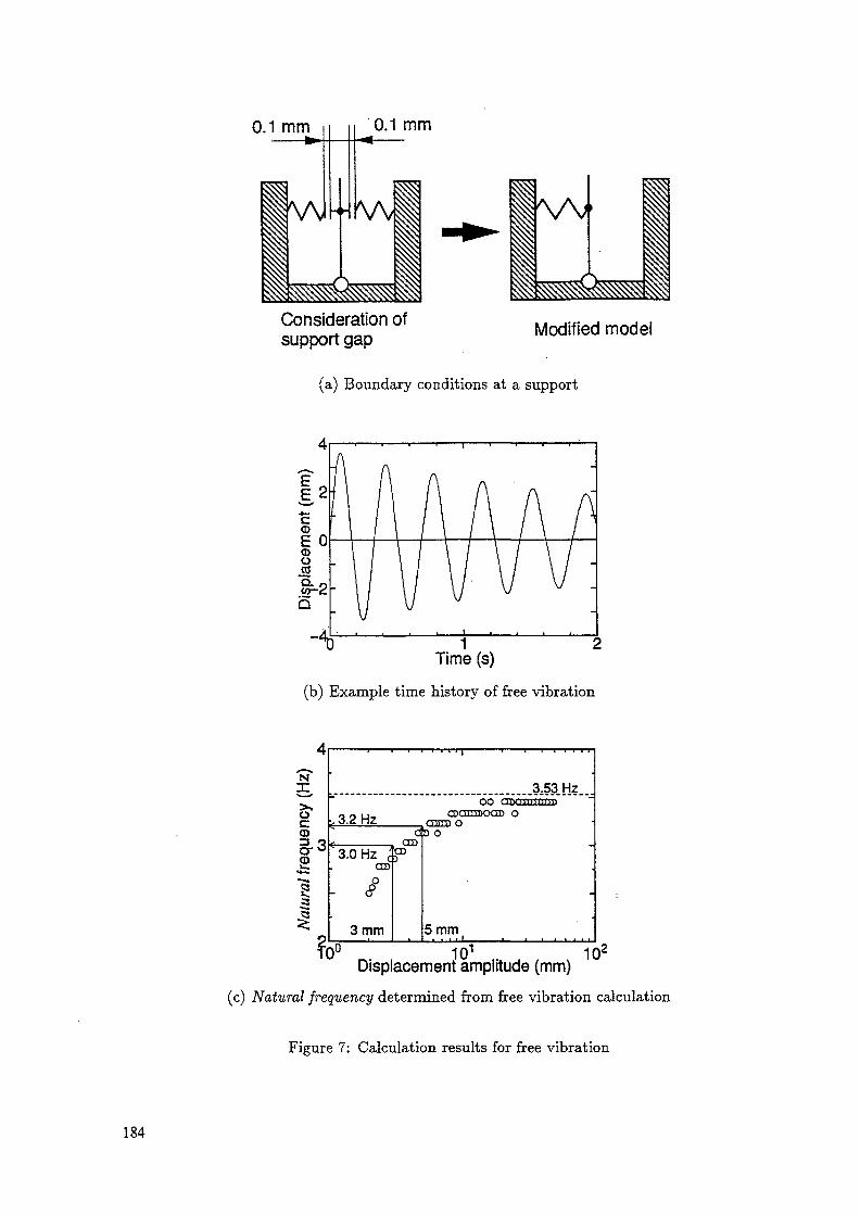
0.1 mm 0.1 mm

r K/vi

Consideration ofsupport gap

hModified model

(a) Boundary conditions at a support

Time (s)

(b) Example time history of free vibration

N

oCD3 -erCD

1

OO

3.2 Hz

3.0 Hz cCCD

do oŒD

3 mm 5 mm'0° 101 10*

Displacement amplitude (mm)(c) Natural frequency determined from free vibration calculation

Figure 7: Calculation results for free vibration

184

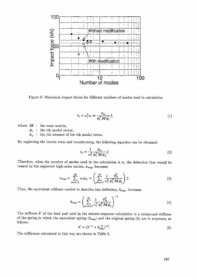
IUU

Z^-^CDÜ

«*—

•5OJQ.E

n

; ' , : : :i i ' >, - . i , • •• , iWithoiT • ' >

-5 Q•Q-V

-t-^ , -; ° Xi<! |With n

! • ' '; ; , ; i : • !

: 1 i ! ! :• 1 : Ml!

it modification i • '<i j i « i | «i ' i , i1 l I !

• • 1 1 - , i .

' !

' ' ! ! '. 1 , i i !

, , : , ,.,.„; , .! ' ! ' 1i ' ! ' i '

lodificatiori ]__ ; { |_i i { I 'M

' i I 'M1 1 ' I , !

10Number of modes

100

Figure 8: Maximum impact forces for different numbers of modes used in calculation

* (1)

where M : the mass matrix,<£j : the îth modal vector,4>13 : the j'th element of the ith modal vector.

By neglecting the inertia term and transforming, the following equation can be obtained:

*>?<tfM<f>t' (2)

Therefore, when the number of modes used in the calculation is n, the deflection that would becaused by the neglected high-order modes, xneg, becomes:

i-neg = E/ oo ,

= V — - (3)

Then, the equivalent stiffness needed to describe this deflection, kneg, becomes:

-1Kn&fj "~" (4)

The stiffness k' of the load pad used in the seismic-response calculation is a compound stiffnessof the spring in which the equivalent spring (kneg) and the original spring (k) are in sequence, asfollows:

The stiffnesses calculated in this way are shown in Table 3.

185

Table 3: Modified stiffnesses of load pads

Number of modes used3456

Kneg117 (MN/m)

96139845185

k' = (1/k + l/kneg)-1

80 (MN/m)190235238

The maximum impact forces using this modified load-pad stiffness are also shown in Fig. 8,in which it can be observed that the modified values gave good acuracy using only four mode,whereas the unmodified-stiffness results only became acceptable using five. It should be noted,however, that the result with the three lowest mode has a large amount of error. This may bebecause the inertia term in the fourth mode should not be neglected. Therefore, the followingseismic- response calculation will be conducted using the four lowest modes with a top-load-padstiffness of 190 MN/m.

3.6 Numerical model used in seismic-response calculations

Given the low number of modes used in the seismic-response calculation, the subassembly modelshown in Fig. 9 is used. The model is valid because the natural frequencies calculated using it areclose to those using the fine- mesh model..

Table 4: Natural frequency calculated by the simplified model

Mode number1234

Simplified3.53 (Hz)

18.8657.28116.61

Fine3.53 (Hz)

18.7657.44116.31

Nodenumber

11Top pad _Added mass2.9kg

Middle pad

Added mass1.0kg

8o

70

Elevation(mm)

42004020

Mass per Flexial stiffnesunit length (kN m2)(kg/m)

"302" 1244

3302

2665

27.2 349

19601218

53.7 349

Disp. - fixed -^Rot. -free~\

5*

2«^-W

; 11^0555

' 51O

. 250i 0

57.9

11.8

790

105

Figure 9: Numerical model used in seismic-response calculations

186

4 CALCULATION FOR SINGLE-ROW EXPERIMENTS

4.1 Description of experiments

In this experiment, twenty-nine subassembly, including seventeen of fuel-assemblies, four of radial-blanket-assemblies, and eight of neutron-shield-assemblies, were arranged in a single row betweenrestraints and excited using a shaking table. The arrangements of the subassembly models areshown in Fig. 10-(a). The measurement points relating to the following discussion are shown inFig. 10-(b). These experiments were conducted both in air and in water.

1 N>d

110.6 mm

^s^^^^^^^^^^s^x^^^^^^^^^N^^^^

oooooooooooooooooooooooooooo 1Vl\V\V^Vs\S\V\V\VV^^^

-^-Direction of excitation

Fuel assmbly model

Blancket assembly model

"Tank

. Restraint

.With orwithoutwater

FR utron shieldmodel

(a) Arrangement of subassembly models

Bar number1 2 3 4 5 6 7 8 9 1011121314151617181920212223242526272829

^OOOOOOOOOOOOOOOOOOOOOOOOOOOOOE1 2 3 4 5 6 7 8 9 10 11 12 13 14 15 16 17 18 192021 22 23 24 25 26 27 28 2930

lmpactforce /Displacement

Position ofstrain measurement

, „\ Strain

(b) Measurement points

Figure 10: Schematic of single-row 29-subassembly experiment

187

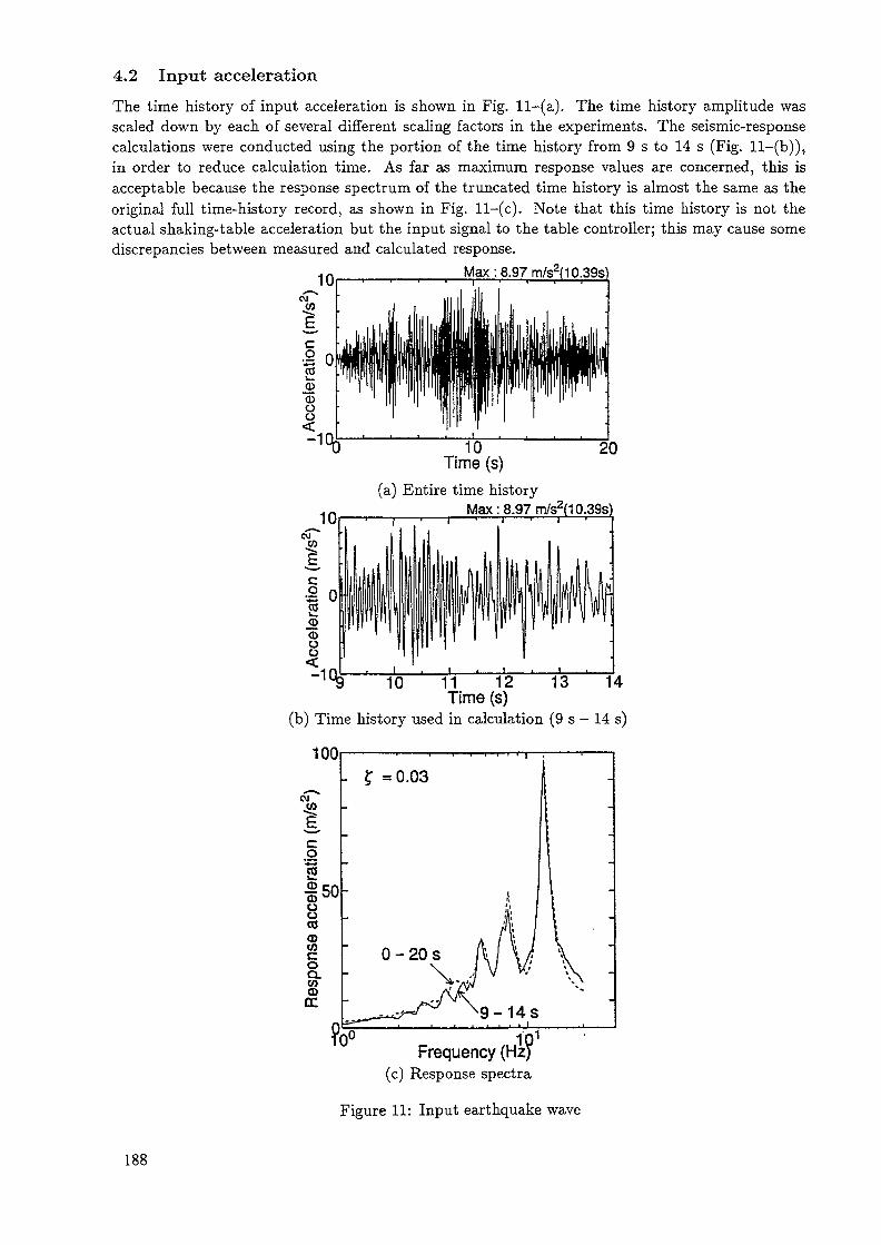
4.2 Input acceleration

The time history of input acceleration is shown in Fig. ll-(a). The time history amplitude wasscaled down by each of several different scaling factors in the experiments. The seismic-responsecalculations were conducted using the portion of the time history from 9 s to 14 s (Fig. ll-(b)),in order to reduce calculation time. As far as maximum response values are concerned, this isacceptable because the response spectrum of the truncated time history is almost the same as theoriginal full time-history record, as shown in Fig. ll-(c). Note that this time history is not theactual shaking-table acceleration but the input signal to the table controller; this may cause somediscrepancies between measured and calculated response.

Max: 8.97 m/s2(10.39s)

10Time (s)

(a) Entire time historyMax: 8.97 m/sz(10.39s)

10 13 1411 12Time (s)

(b) Time history used in calculation (9 s - 14 s)

100

1Q1

Frequency (Hz)(c) Response spectra

Figure 11: Input earthquake wave

188

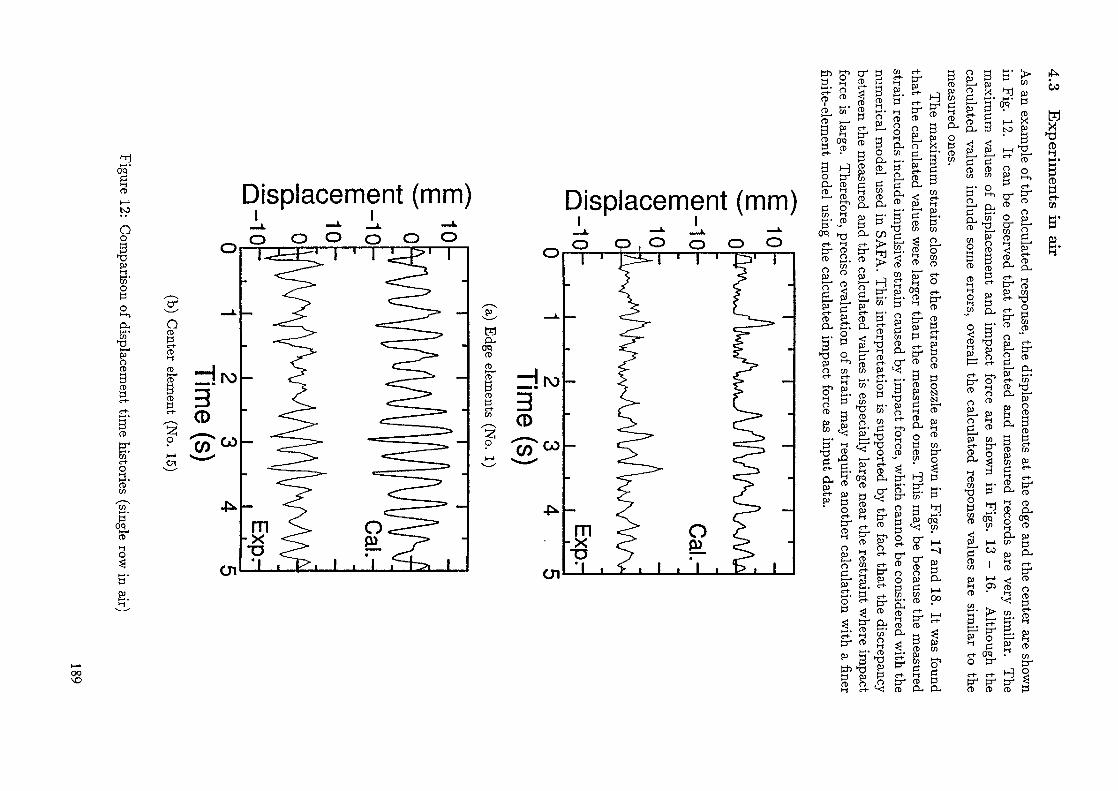
to

OoI

opo1-nCL.5)'

T3p"On>

3etEen"et-Ot-jet'cn

cnB'

n>HO

Displacement (mm) Displacement (mm)

OetPet-et^etet"

gg-

^O

et ,—a PS "•!2 <wP etc-t- •

3 H0 p-CL, et

0 S1en HS'-«irf- 1-t

ft" B.

g S

eT 2a £8- H*ST P

3 p>o oP 1-4O enet- et-

o1 S.

—B H•S ga

er Pet £

î let 2.P O«* ELof 3

g S-p £.S *Pi enet 5CL, CL,P 3'P D

CL. enet- >>

^£O

0)C-+-

3Bi-ietoonCL.cnP-oETCL,et

B'

S tr£ï.et p°- S"<! HPL 0 etet £•en P>-• £?;cn Qet P» ^.

^3 en

B. gP. -spî c-l-i-i et

(K) CL,

1^-fa et-H P;et- «tr w,et pr3 »en et-fT ^S. 8P. et.

^ ^ SîS-' H gtr et o^ i'-s3^ g

etoog£eti-ietCL,

P"et

P-P

-0r^g.1o X£• 3'^ 5et- P(t pCL, &< g-8L 3eS 3"en en< a1 5"2 enet et

8 eT? etpT Pp ET•* Sirr1 P» e?3 PS oP tsi§ £.M et

^ ^O »P enS eT

3 33 <8^^er p« ICD CL.

eg 00

g. t-HeT rt'P ^P pet cn

1 s»^ set PCL. CL.

P °S t°et >—•ûj OIn P

ilo ^D0- CL,I Ieten

POletcnO

§etMI-!O

K

i s ->«. 3 ga OT P

g - S3 to P< ' 3P i—< 'o^ ^ sret e-> oen P S,0 £1l~h er 5^^ " o»-.. ocn O pi

>Ö er ï-1

P jg Ss ^ r3 I et2 °-g- &• sg ?|§ - ^ gs- r sP O "*u eu et-p g- p"O p et

P" get 3o «&. pO H3- ^pT1 enet- o-

S,|>i Pet3 B'§ ^d^-

F w

^ ïP >-;1-1 CJiet •

3

S §et- OTO p-

P" P4

et et

p Ctet- cnet X)

^efs §°-g3 g-et enen PC ^S =•*-a-efet Ä

8 § "CL, jacn gp CL,8 £5 ro

à S

I.Pl'a

enP"

-Iet P

aX13(BH

P

B-

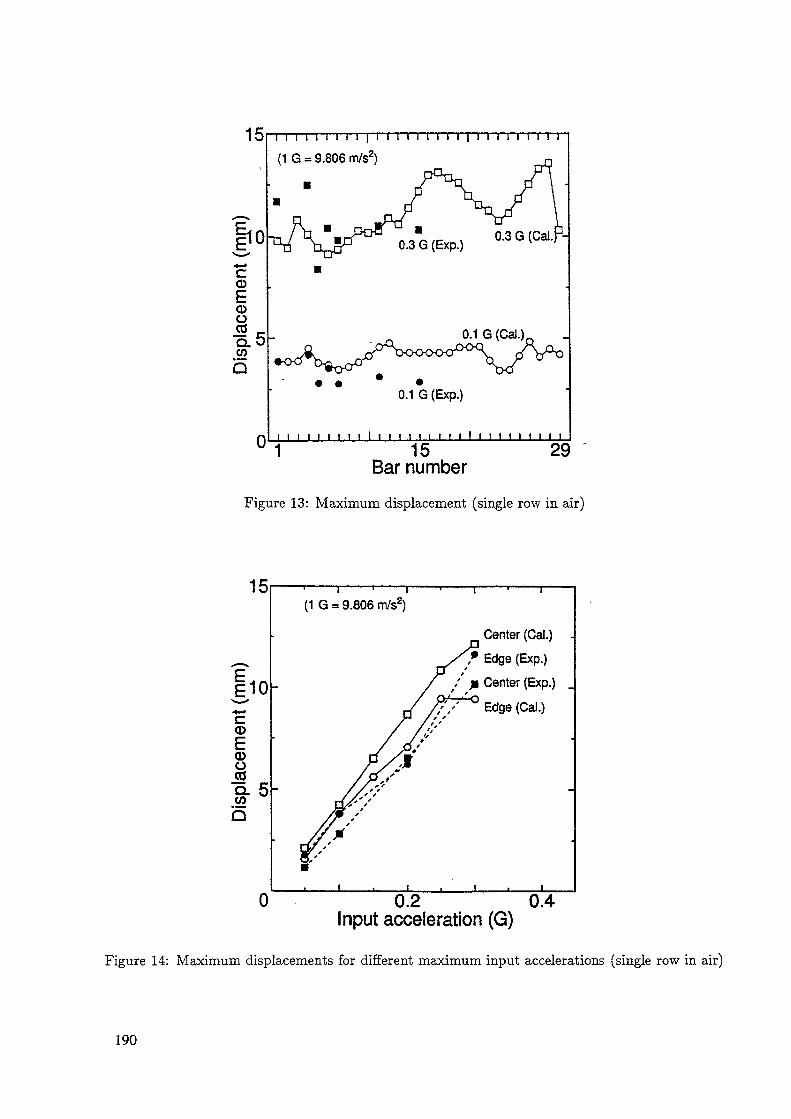
15

^—•x

|o03

CDÜ&0.CO

0

(1 G = 9.806 m/s2)

0.1 G (Cal.).

0.1 G (Exp.)

i i i i i i i i l i i i i i i i i i I i i i i i i1 15 29

Bar numberFigure 13: Maximum displacement (single row in air)

15

cCD

(DÜCOQ. 5COQ

0

(1 G = 9.806 m/s2)

Center (Gal.)

r Edge (Exp.)

.' p Center (Exp.)

Edge (Cal.)

0.2 0.4Input acceleration (G)

Figure 14: Maximum displacements for different maximum input accelerations (single row in air)

190

20

CD

o10

Q.

i i i i i i i i i | i i i i i n i i i i n i i i i i i iTop pad

0.3 G (Exp.)0.3 G (Exp.)

i i i i i i i i i M i i i i i i i i l i i i i i i i i i

Impact point number

Figure 15: Maximum force (single row in air)

20 . (1 G = 9.806 m/s2)

^CD

COCL

Top padNo.1 (Cai.)

No.1 (Exp.)

/ / No.30 (Exp.)

No.30 (Cal.)

Middle padNo.1 (Cal.)

lo.SO (Cal.).1 (Exp.)

No.30 (Exp.) -

0.2 0.4Input acceleration (G)

Figure 16: Maximum force for different maximum input accelerations (single row in air)

191

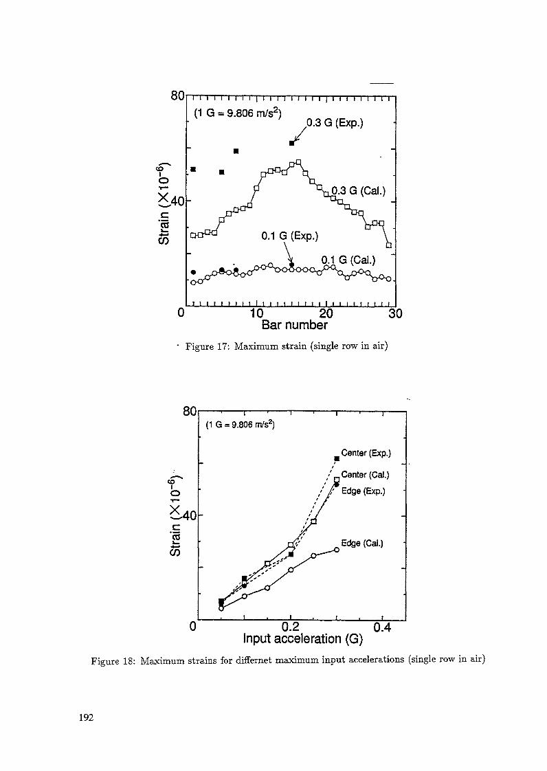
80

CO

X.40

205

(1 G = 9.806 m/s2),0.3 G (Exp.)

3 G (Cal.)

0i i i i i i i i i l i i i i i i i i i!_i_i_..i_i_r JU i

10 20Bar number

30

" Figure 17: Maximum strain (single row in air)

80

<obXcs+~*co

40

(1 G = 9.806 m/s2)

Center (Exp.)

/ 'Center (Cal.)/ /Edge (Exp.)

Edge (Cal.)

0 0.2 0.4input acceleration (G)

Figure 18: Maximum strains for differ net maximum input accelerations (single row in air)

192

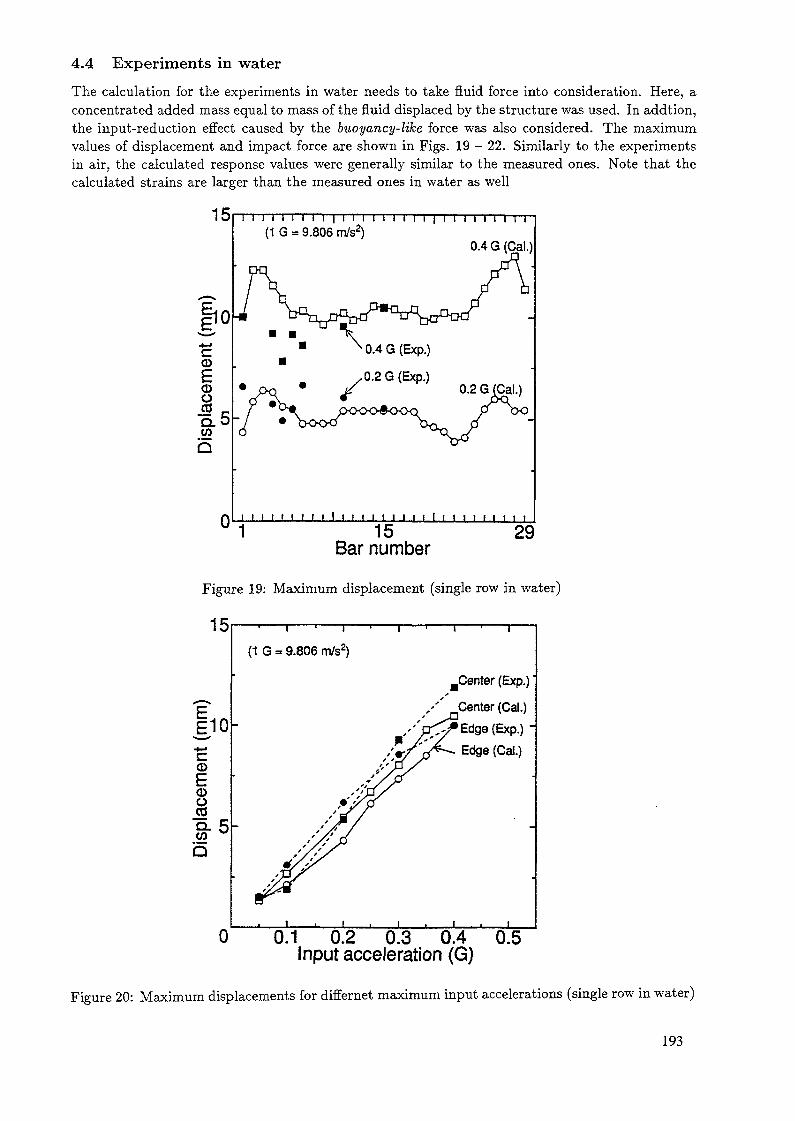
4.4 Experiments in water

The calculation for the experiments in water needs to take fluid force into consideration. Here, aconcentrated added mass equal to mass of the fluid displaced by the structure was used. In addtion,the input-reduction effect caused by the buoyancy-like force was also considered. The maximumvalues of displacement and impact force are shown in Figs. 19 - 22. Similarly to the experimentsin air, the calculated response values were generally similar to the measured ones. Note that thecalculated strains are larger than the measured ones in water as well

15

*•—xioCDCDO&0.CO

l l l M I I II | I I I I I I II I |(1 G = 9.806 m/s2)

l l i l i i l l l

0.4 G (Cal.)

k 0.4 G (Exp.)

,0.2 G (Exp.)

i i i i i i i i i l i i i i i i i i i l i i i i i i i i i15

Bar number29

Figure 19: Maximum displacement (single row in water)

15

^—^

I«••—«CD

CDÜcd"5. 5wb

(1 G = 9.806 m/s2)

Renter (Exp.)

Center (Cal.)Edge (Exp.) 'Edge (Cal.)

0 0.1 0.2 0.3 0.4 0.5Input acceleration (G)

Figure 20: Maximum displacements for differnet maximum input accelerations (single row in water)

193

20

oio

o.

0

0.4 G (Exp.) (1 G = 9.806 m/s2)Top pad

0.4 G (Exp.).

oo00 0.2G(Exp.>i i i i i i i i i i i i i i rimpact point number 30

Figure 21: Maximum force (single row in water)

20

oo010

Q.

(1 G =» 9.806 m/s2) Top padNo.1 (Exp.)

^

No.1 (Cal.)

No.30 (Exp.

No.30 (Cai.)

Middiepad_No.30 (Gal.)No.1 (Gal.)No.30 (Exp.)

""* No.1 (Bp.)"0.1 0.2 0.3 0.4 0.5

Input acceleration (G)

Figure 22: Maximum forces for different maximum input accelerations (single row in water)

194

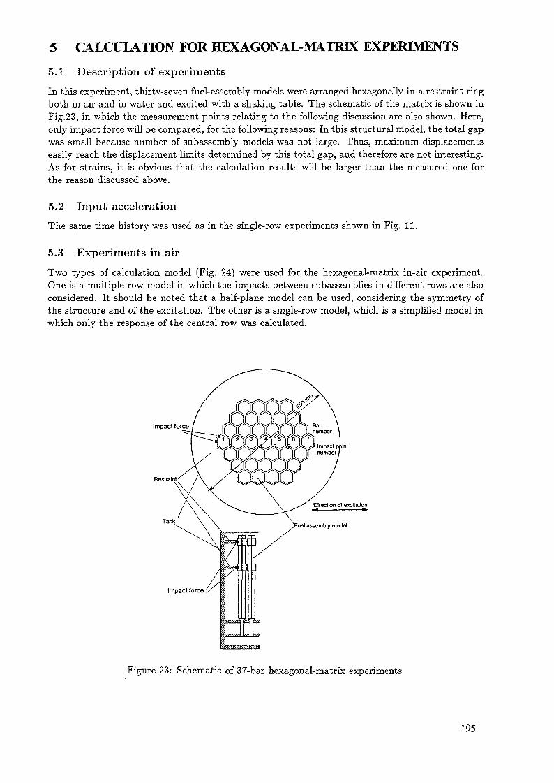
5 CALCULATION FOR HEXAGONAL-MATRIX EXPERIMENTS

5.1 Description of experiments

In this experiment, thirty-seven fuel-assembly models were arranged hexagonally in a restraint ringboth in air and in water and excited with a shaking table. The schematic of the matrix is shown inFig.23, in which the measurement points relating to the following discussion are also shown. Here,only impact force will be compared, for the following reasons: In this structural model, the total gapwas small because number of subassembly models was not large. Thus, maximum displacementseasily reach the displacement limits determined by this total gap, and therefore are not interesting.As for strains, it is obvious that the calculation results will be larger than the measured one forthe reason discussed above.

5.2 Input acceleration

The same time history was used as in the single-row experiments shown in Fig. 11.

5.3 Experiments in air

Two types of calculation model (Fig. 24) were used for the hexagonal-matrix in-air experiment.One is a multiple-row model in which the impacts between subassemblies in different rows are alsoconsidered. It should be noted that a half-plane model can be used, considering the symmetry ofthe structure and of the excitation. The other is a single-row model, which is a simplified model inwhich only the response of the central row was calculated.

Impact force

Restrain!

Tank

OuOQf

Impact force

Figure 23: Schematic of 37-bar hexagonal-matrix experiments

195

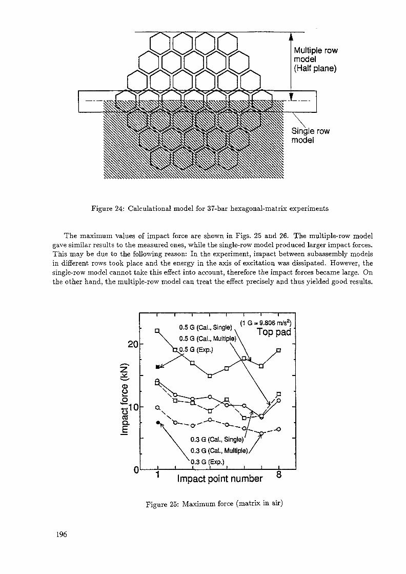
OÜÜOncrom

Multiple rowmodel(Half plane)

Single rowmodel

Figure 24: Calculational model for 37-bar hexagonal-matrix experiments

The maximum values of impact force are shown in Figs. 25 and 26. The multiple-row modelgave similar results to the measured ones, while the single-row model produced larger impact forces.This may be due to the following reason: In the experiment, impact between subassembly modelsin different rows took place and the energy in the axis of excitation was dissipated. However, thesingle-row model cannot take this effect into account, therefore the impact forces became large. Onthe other hand, the multiple-row model can treat the effect precisely and thus yielded good results.

20

CDO

COQ.

0

0.5 G (Cal.. Single) (1 G = 9.806 m/s2)Top pad

o-

7-

.0.3 G (Exp.)

j___i___i___i

-O

Impact point number 8

Figure 25: Maximum force (matrix in air)

196

30

200>£££"o

I I

(1 G = 9.806 m/s2)Top

Cal. (Single)Exp.Cal. (Multiple)

Middle _Cal. (Single)

Exp.aaCal. (Multiple)

0 0.2 0.4 0.6 0.8Input acceleration (G)

Figure 26: Maximum forces for différent maximum input accelerations (matrix in air)

5.4 Experiments in waterFor this calculation, three types of models with different structural modeling and fluid-force model-ing were used. As for structural modeling, the same multiple-row and single-row models were usedas in the in-air experiment. For fluid-force modeling, an added-mass matrix and a concentratedadded mass were used. As discussed in Section 2, the former can take fluid/structure interactioninto account, while the latter is a simplified model which can simulate only the predominant mode.The three calculation models are summarized in Table 5. Note that for the single-row model noadded-mass matrix exists. The concentrated added mass coefficient1 was calculated to be 1.03 byusing a method reported elsewhere [8]. The input-reduction effect by the buoyancy-like force wasalso taken into account.

Table 5: Calculation models

StructureMultiple row

Single row

Fluid force modelAdded mass matrix

Model A—

Concentrated massModel BModel C

The maximum values of impact force are shown in Figs. 27 and 28.First, let us compare the three calculation models. With the concentrated mass models (Model

B, C), the impact forces for the single-row model (Model C) were larger than those for the multiple-row model (Model B) — this is the same as the in-air result. With the multiple-row models (ModelA, B), the impact forces from the concentrated added mass (Model B) were larger than those fromthe added mass matrix model (Model A). This can be understood as follows: The fluid/structureinteraction considered in Model A, makes the subassembly models vibrate in-phase and thus reducesthe amount of impact interaction between subassembly models in different rows. Therefore, theenergy dissipation in the excitation direction becomes small.

197

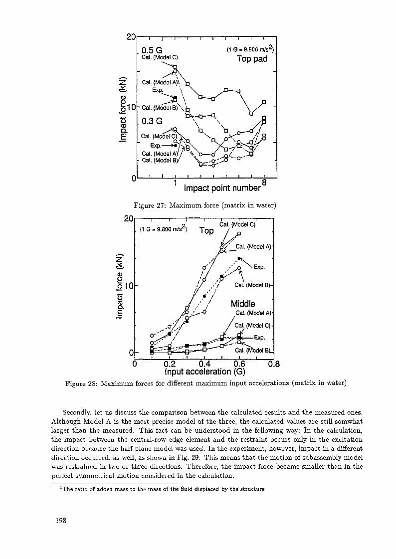
20

CD

§10oCOQ.

0

' 1 ' r

0.5 GCal. (Model C)

Cal. (Model A)\ExP;

- Cal. (Model

0.3 GCal. (Moclel

Exp.Cal. (ModelCal. (Model B

(1 G - 9.806 m/s2)Top pad

1 8Impact point number

Figure 27: Maximum force (matrix in water)

20. (1 G = 9.806 m/s )

<DÜ510

a.

0

Cal. (Model C)

.(Model A)

// /^"// // Cal. (Model B)-

'' / MiddleCal. (Model A)-

Cal. (Model C)

Exp.

Cal. (Model B),i___i___i

0 0.2 0.4 0.6 0.8Input acceleration (G)

Figure 28: Maximum forces for différent maximum input accelerations (matrix in water)

Secondly, let us discuss the comparison between the calculated results and the measured ones.Although Model A is the most precise model of the three, the calculated values are still somwhatlarger than the measured. This fact can be understood in the following way: In the calculation,the impact between the central-row edge element and the restraint occurs only in the excitationdirection because the half-plane model was used. In the experiment, however, impact in a differentdirection occurred, as well, as shown in Fig. 29. This means that the motion of subassembly modelwas restrained in two or three directions. Therefore, the impact force became smaller than in theperfect symmetrical motion considered in the calculation.

lrThe ratio of added mass to the mass of the fluid displaced by the structure

198

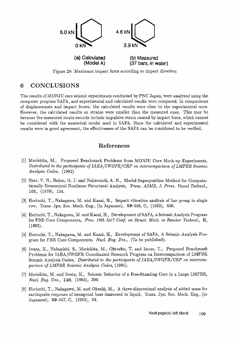
6.0 kN I I 4.6 kN

3.9 kN

(a) Calculated (b) Measured(Model A) (37 bars, in water)

Figure 29: Maximum impact force according to impact direction

6 CONCLUSIONSThe results of MONJU core seismic experiments conducted by PNC Japan, were analyzed using thecomputer program SAFA, and experimental and calculated results were compared. In comparisonsof displacements and impact forces, the calculated results were close to the experimental ones.However, the calculated results on strains were smaller than the measured ones. This may bebecause the measured strain-records include impulsive strain caused by impact force, which cannotbe considered with the numerical model used in SAFA. Since the calculated and experimentalresults were in good agreement, the effectiveness of the SAFA can be considered to be verified.

References

[1] Morishita, M., Proposed Benchmark Problems from MONJU Core Mock-up Experiments,Distributed to the participants of IAEA/IWGFR/CRP on intercomparison of LMFBR SeismicAnalysis Codes, (1992).

[2] Shar, V. N., Bohm, G. J. and Nahavandi, A. N., Modal Superposition Method for Computa-tionally Economical Nonlinear Structural Analysis, Trans. ASME, J. Press. Vessel Technol.,101, (1979), 134.

[3] Horiuchi, T., Nakagawa, M. and Kasai, H., Impact vibration analysis of bar group in singlerow, Trans. Jpn. Soc. Mech. Eng., (in Japanese), 59-559, C, (1993), 650.

[4] Horiuchi, T., Nakagawa, M. and Kasai, H., Development of SAFA, a Seismic Analysis Programfor FBR Core Components, Proc. 12th Int'l Conf. on Struct. Mech. in Reactor Technol., E,(1993).

[5] Horiuchi, T., Nakagawa, M. and Kasai, H., Development of SAFA, A Seismic Analysis Pro-gram for FBR Core Components, Nucl. Eng. Des., (To be published).

[6] Iwata, K., Nakanishi, S., Morishita, M., Ohtsubo, T. and Inoue, T., Proposed BenchmarkProblems for IAEA/IWGFR Coordinated Research Program on Intercomparison of LMFBRSeismic Analysis Codes, Distributed to the participants of IAEA/IWGFR/CRP on intercom-parison of LMFBR Seismic Analysis Codes, (1991).

[7] Morishita, M. and Iwata, K., Seismic Behavior of a Free-Standing Core in a Large LMFBR,Nucl. Eng. Des., 140, (1993), 309.

[8] Horiuchi, T., Nakagawa, M. and Ohashi, M., A three-dimensional analysis of added mass forearthquake response of hexagonal bars immersed in liquid, Trans. Jpn. Soc. Mech. Eng., (inJapanese), 59-557, C, (1993), 93.

Next page(s) left blank 199

FINAL REPORT ON RESULTS OFCALCULATIONS BY CORE-SEIS

R. RAVI, P. CHELLAPANDI, T. SELVARAJ,S.C. CHETAL, S.B. BHOJENuclear Systems Division,Indira Gandhi Centre for Atomic Research,Kalpakkam, India

Abstract

Under the Coordinated Research Program on 'Intercoraparison of LMFBR seismicanalysis codes' organised by IAEA/IWGFR, benchmark analysis using theexperimental data supplied by France, Italy and Japan have been carried outin order to verify and validate the computer codes developed for the coreseismic analysis. In this context, the special purpose computer code 'CORE-SEIS' has been developed at IGCAR, Kalpakkam, which has many novel featuresso as model the complex phenomenon that are associated with the seismicmotions of LMFBR subassemblies. The analysis has been performed for thefollowing cases.

Rapsodie (France) tests on free standing core in air and water.PEC (Italy) data on :

i) tests with single PEC fuel subassembly (in air and water)ii) teats with a small cluster (7 and 19 subassemblies) inair and water.

Monju (Japan) data on:i) impact and vibration tests on single subassemblyii) vibration tests on 37 subassembly cluster and 29subassemblies in a row.

Most of the experimental results are satisfactorily predicted by CORE-SEIS.The CORE-SEIS predictions also have shown good comparison with other coreseismic analysis codes used in the CRP.

1. INTRODUCTION

The core of a Liquid Metal Fast Breeder (LMFBR) is composed of severalhundreds of subassemblies of different kinds such as fuel, blanket andneutron shield subassemblies. They are self-standing hexagonal beamssupported on rigid structure called core support structure (CSS). The coreis completely immersed in liquid sodium with narrow spacings betweenadjacent assemblies.

In an earthquake event, the whole cluster of core subassemblies willbe experiencing a complicated vibratory motion due to nonlinearityintroduced by the collisions between the subassemblies and dynamicinteraction through fluid coupling forces. The vibratory motions ofsubassemblies are very crucial in an LMFBR due to their effects on theinsertability of control rods (CRs) for tripping the reactor and thereactivity addition aspects. The possible vibratory motions in thevertical and horizontal directions as well as radially inward and outwarddirections cause 'vertically oscillatory', 'beam bending type' and'flowering' modes respectively. If there is a mismatch between thecontrol rods and crest of subassemblies in the horizontal direction abovecertain limit (20-25mm), there may be a problem of insertability of CRs

201

during an earthquake (Fig.la). Since the reactor assembly of an LMFBR isvertically supported at the top, the CRs which are mounted on the top roof,will be withdrawn/inserted into reactor core under vertical motionsresulting in an addition/reduction of reactivity (Fig.lb). The movements ofcore radially inward (flowering motions towards the central zone whereneutron flux is high) as seen in Fig.lc, also cause the possibility ofreactivity addition.

Roof slab

Control Rod

Main V*s3«i

Core sub-assembly

CSS

(i) Mismatch due to relative horizontal motions

Withdrawal of CR

(ii) Reactivity insertion due to vertical motions

Flowering

(iti) Reactivity insertion due to radially inward motions".

Rg.l Effect of seismic motions on safety of LMFBR

202

Since the reactivity worth of LMFBR control rods is high (~1pcm/mm/rod) , a few mm movement itself is very crucial. Further theneutronic events are much faster than the time scale involved in theseismic motions, there is sufficient time available for the build up ofreactivity due to vibratory motions of the core during an earthquake event.Hence an accurate assessment of dynamic response of the subassemblies andalso their structural integrity is very important from the safety point ofview. This requires a well validated large scale non-linear dynamicanalysis methodology. In this context, a special purpose inhouse computersoftware called 'CORE-SEIS' has been developed. The code has been providedwith many novel features to have the capabilities to model the complexphenomenon that are associated with seismic motions of LMFBR subassembliesand also has ability to solve with reasonable amount of computer time.Some of the international codes available for this purpose are dealt inrefences [1-4].

2 . STATE-OF-THE-ART REVIEW OF THE SEISMIC EXPERIMENTAL AND ANALYTICAL WORKAT IGCAR

2.1. Seismic analysis methodology

The proposed site for the 500 MWe Prototype Fast Breeder Reactor{PFBR) is Kalpakkam which is situated in the low seismic zone. The siteseismicity for the Kalpakkam site is 0.176 g. The seismic analsyis of thePFBR rector assembly is performed in 2 phases. In the first phase, a timehistory analysis using spectrum compatible accelerograms is performed onthe 'stick' model comprising of base raft, reactor vault, reactorcontainment building. (RGB), reactor containment etc (Fig.2) [5-6]. Thefloor response spectrum is generated from the response at the roofslablevel, which is used in the second phase for the response spectrum analysisof an axisymmetric model of the reactor assembly including the fluidstructure interaction. Components like roofslab and core support structurewhich have radial stiffeners violating the axisymmetry are modelled by anaxisymmetric ring with negligible tangential stiffness using theorthotropic material modelling.

As for the experimental works, the dynamic experiments on the 1/3Othmodel of the main vessel has been carried out and the natural frequenciesof the structure in air and water filled condition were obtained using themodal shaker. The comparison between the calculated natural frequencies isgood except for the beam bending mode. The dynamic experiments on thel/15th model of the main vessel are on the anvil.

The shake table experiments on the 1.5 m tall bottom supported waterfilled Aluminium tank is being conducted to study the contribution of theshell modes in the seismic response. Significant shell bending modes (outof roundness circumferencial modes) have been observed during thehorizontal base excitation at various frequencies. The experiments are inthe advanced stage of completion.

Experiments on core subassemblies are also proposed with increasingcomplexity in the impact behaviour of the subassemblies.

2.2. Core seismic analysis

As for the core seismic • response, the response time history at the topsurface of CSS, is used as the input for the subsequent core seismicanalysis. In the first phase calculations, the mass inertia and stiffnessvalues of the subassemblies are accounted by introducing a single compositebeam. This means that the beam bending type deformation behaviour is onlyconsidered without introducing any complex nonlinear effects. In the

203

—RGB

ROOFSLAB SKIRTMAIN VESSEL

ss

Kv-CONCRETE VAULT

t%7

MODEL FOR HORIZONTAL EXCITATION MODEL FOR VERTICAL EXCITATION

Fig2. St ick model

second, phase more realistic motions are computed by time history analysis,including all the possible complexities. It is to be noted that the stickmodel is different for horizontal and vertical excitations because of thedifference in the supporting and inertial characteristics of the reactorassembly components as a whole.

2.3. Modelling complexities

Each fuel and blanket subassemblies in the core consists of many smallclad tubes and fuel pins surrounded by liquid sodium within an outerhexagonal sheath. This causes uncertainties in simulation of correctstiffness and mass effects. The uncertainity is still more for thesubassemblies which are seeing the end of life because of the effectsof the deformation of fuel pins due to neutron irradiation.Since each subassembly is free standing the boundary condition atsupport is very difficult to define (Fig.3) . It is neither fixed norsimply supported.Each subassembly is separated from the surrounding ones with small gapat intermediate loading pad locations (usually at one or two locationsalong the length, refer Fig.4). This produces strong non-linearity dueto change of contact conditions in the course of vibratory motion.Another difficulty is the definition of gap distribution at the startof an earthquake.Fluid structure interaction effects due to surrounding sodium aroundsubassembly.Definition of global damping values and also local damping at theloading pads.large size problem due to 3D aspects of core configuration which callsfor 180 deg. sector model for the analysis.

204

Ncoe2

Nooei

(a) AsmaJesLpoortard'scnngs (b) A sanoie sunport and scrngs witft gans

Fig.3 Boundary condition model

3. DESCRIPTION OF THE CORE SEISMIC ANALYSIS CODE 'CORE-SEIS'

3.1. Modelling features

Each, subassembly is treated as a 3D beam with different moment ofinertia and mass per unit length depending upon the internal structuresand configuration.The loading pads are modelled by a linear spring and a dash pot inassociation with the required gap (Fig.5).The supporting conditions at the foot of the subassembly are introducedby the springs with appropriate stiffness values so as to simulate thenatural frequency values observed experimentally.FSI effects are modelled using added mass concept both for internal andexternal sodium coolant.The global damping is introduced by defining modal damping coefficients(a,b) which are determined based on two natural frequencies ofinterest.

Fig.4 Loading pad details

205

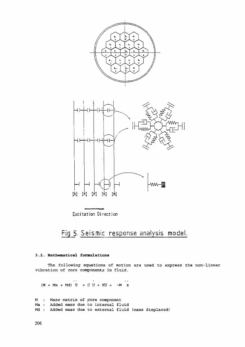
Hf-

-ih-

-1

d t>

Hf-

HK

-t

d l>

—\\-r

HM1 1 \

Ç

(] I?

^^**"

^^^

s~~

H^N .

_-^

<1

Excitation Direction

Fig 5. Seismic response analysis model.

3.2. Mathematical formulations

The following equations of motion are used to express the non-linearvibration of core components in fluid.

(M + Ma + Md) U + C U + K U = -M z

M : Mass matrix of core componentMa : Added mass due to internal fluidMd : Added mass due to external fluid (mass displaced)

206

C : Damping matrixK : Stiffness matrixU : Relative displacement vector with respect to support motionz : Support motion (seismic excitation)

The damping matrix is calculated by Rayleigh Damping model, using thefractions of critical damping for the first and second vibration mode.

In order to model the collision between subassembly, the stiffness andthe damping matrix are updated using the shock stiffness (Kc) and the shockdamping (Cc) at the appropriate locations corresponding to the degree offreedoms that are associated with the node at which the collision occurs.The collision stiffness matrix and the damping matrix are:

Kc -Kc Cc -Cc; [C]shock-Kc Kc -Cc Cc

[K]shock ~ ; [C]shock

The [K] shoci- and the [C] g^or-v are added to the global stiffness matrix[K] and damping matrix [C] respectively only when a gap closes.

The above equations of motions are solved using the Newmark-b method.At the begining of the solution step, the inequality for the gap closercondition is checked to accordingly modify the global stiffness and dampingmatrices. The solution is sought explicitly and hence no iterations areneeded for shock force calculations due to collision. Even though manysophisticated implicit algorithms are available to accurately model thecollision phenomena, the explicit technique is preferred to get anoptimum solution with reasonable computer time.

4. SUMMARY OF WORK DONE AT IGCAR ON CRP DURING 1990-95

The code CODE-SEIS has been developed during this period. As a part ofthe Coordinated Research programme, the three different analysis have beenperformed for the experimental data supplied by the countries France, Italyand Japan respectively by which the performance of the code CORE-SEIS hasbeen validated.

4.1. French data

1) Natural frequency determination of fuel sub-assemblies by assumingpinned support condition at the nodes corresponding to the top andbottom support plate.

2) Natural frequency determination by time history analysis by modelingthe gap between the sub-assembly and the diagrid.

3) Seismic response of central row of the mock up composed by 11 fuelassemblies and 8 neutronic shield elements in air.

4.2. Italian data

1) Natural vibration behaviour of single fuel and reflector S/A2) Response of a single fuel subassembly subjected to base random

excitation3} Response of 7 fuel SA configuration subjected to base excitation4) Response of 19 fuel subassembly configuration subjected to random base

excitation5) Response of 19 fuel and reflector subassembly configuration subjected

to base seismic excitation

207

4.3. Japanese data

1) Natural frequency analysis for single assembly2} Collision analysis for single assembly model3) Seismic response for single row configuration (29 sub-assemblies) - In

air4) Seismic response for single row configuration (29 sub-assemblies) - In

water5) Seismic response for cluster configuration in Matrix layout (37 sub-

assemblies) - In air6) Seismic response for cluster configuration in Matrix layout (37 sub-

assemblies) - In water

In all these cases the results of the calculation were in goodagreement with the experimental values.

5. RESULTS OF VALIDATION, VERIFICATION AND IMPROVEMENTS OF THE CORE-SEISUSING THE EXPERIMENTAL DATA

Since the calculations were performed for three different experimentaldata, the relevant results of the calculations and their comparisons withthe experiment are given separately.

5.1. Results of calculations with. French data

Rapsodie core mock up is composed of 91 fuel assemblies located atthe centre of the mock up (1 central assembly and 5 rings) surrounded by180 neutronic shield elements (4 rings). Since the total number ofsubassemblies in the cluster lay-out is 291, the total CPU time estimatedfor having a single result, for the cluster lay-out, will be more than 30days in PC 486 computer. Hence the analysis was done for the central row ofsubassemblies and the results of calculations are given here.

5.1.1. Eigen value analysis

The natural frequencies were found by both linear eigen value analysisand non-linear time history analysis.

In the linear eigen value analysis, the calculated natural frequencyfor the fuel sub-assembly in air with pinned support condition is 8.14 Hzwhich is 2% higher than the experimentally observed natural frequency of8.0 Hz.

In the non-linear time history, the natural period of vibration wasfound out from the tip displacement response history which is 0.1333 s.The natural frequency corresponding to this is 7.6 Hz which is 5% lessthan the experimentally observed value of 8.0 Hz.

5.1.2. Seismic calculations

The seismic calculations were performed for the 'Model A' whichrepresents the central row (diameter) of the mock-up composed by 11 fuelelements and 8 neutronic elements. The tip displacement response for allthe 19 subassemblies in the row were obtained. Four typical comparisonplots, three for fuel sub-assemblies and 1 for shielding sub-assembly areshown in the Fig. 6 to Fig. 9. From the Figures, it can be seen that the

208

E

20.00 -

15.00 '-

10.00 -

C 5.00

O.ÛOCL<£ -5.00-Q

-10.00 -

-15.00 -

-20.00

exptcore—seis

0.00 1.00 2,00 3.00TIME

COMPARISON OF DISPLACEMENT AT LOC.7IN AIR TEST. (ROW MODEL)

Fig.6

exptcore—seis

20.00 -i

0.00 -----

O

-20.000.00 3.001.00 2.00

Time (s)COMPARISON OF DISPLACEMENT AT LOC.8

IN AIR TEST. (ROW MODEL)

Fig.7

209

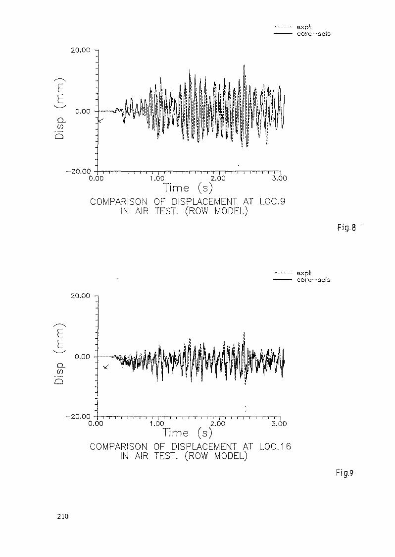
exptcore—seis

20.00 -,

EJE,CL

5

0.00 -—-<•

-20.00 T—I—I—I—t—I—I—1—I—|—I—I—I—I—I—I—1—I—r~|—I—1—I—I—I—I—I—I—I—!

0.00 1.00 2.00 3.00Time

COMPARSON OF DISPLACEMENT AT LOG.9IN AIR TEST. (ROW MODEL)

20.00 -,

EECLc/2Q

0.00 -----

-20.000.00

i j I I I I ! I I I I [ T

1.00 2.00 3.00

Fig.8

exptcore—seis

Time (s)COMPARISON OF DISPLACEMENT AT LOC.16

IN AIR TEST. (ROW MODEL)

Fig.9

210

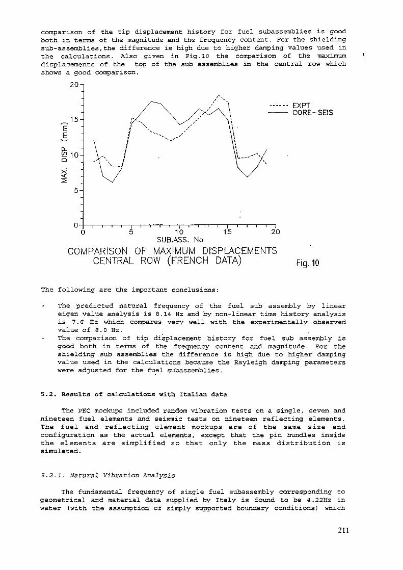
comparison of the tip displacement history for fuel subassemblies is goodboth in terms of the magnitude and the frequency content. For the shieldingsub-assemblies,the difference is high due to higher damping values used inthe calculations. Also given in Fig.10 the comparison of the maximumdisplacements of the top of the sub assemblies in the central row whichshows a good comparison.

20-1

a.<£ 10-Q

5-

0-0 10

i15

EXPTCORE-SEIS

20SUB.ASS. No

COMPARISON OF MAXIMUM DISPLACEMENTSCENTRAL ROW (FRENCH DATA) Fig.10

The following are the important conclusions :

The predicted natural frequency of the fuel sub assembly by lineareigen value analysis is 8.14 Hz and by non-linear time history analysisis 7.6 Hz which compares very well with the experimentally observedvalue of 8.0 Hz .The comparison of tip displacement history for fuel sub assembly isgood both in terms of the frequency content and magnitude. For theshielding sub assemblies the difference is high due to higher dampingvalue used in the calculations because the Rayleigh damping parameterswere adjusted for the fuel subassemblies.

5.2. Results of calculations with Italian data

The PEC mockups included random vibration tests on a single, seven andnineteen fuel elements and seismic tests on nineteen reflecting elements.The fuel and reflecting element mockups are of the same size andconfiguration as the actual elements, except that the pin bundles insidethe elements are simplified so that only the mass distribution issimulated.

5.2.1. Natural Vibra tion Analysis

The fundamental frequency of single fuel subassembly corresponding togeometrical and material data supplied by Italy is found to be 4.22Hz inwater (with the assumption of simply supported boundary conditions) which

211

is higher than the experimental value of 3.2Hz. Hence certain adjustmentson boundary condition have been made to match with experimentalobservations on the natural modal behaviour so that the comparison ofresponses by base excitations will be more meaningful. This has beenachieved in line with^ the approach followed by TOSHIBA.

5.2.2. Response Analysis of Single Fuel Subassembly for Random InputExcitations

The overall comparison• is quite satisfactory with respect to peakvalues. However, point by point comparison is impossible with the timehistories. Hence comparisons are made in frequency domain. The Fouriertransforms of responses (Accelerations) and also amplification factors(output/input} have been compared which showed a reasonble comparison.

5.2.3. Response Analysis of 7 Fuel Subassembly Configuration for RandomInput Excitations

Since all the 7 fuel subassemblies are identical in all the respects,theoretically it is expected that the response of single subassembly andthat of 7 subassembly case will be identical. But in reality due topossible variations in the supporting conditions, the individual behaviourmay not be identical which may cause relative displacements amongsubassemblies, changing with respect to time and thus leading to furthercomplex interactions due to impacts at load pads. Since modelling of suchuncertainties associated with the supporting conditions are nearlyimpossible, an attempt is made by assuming 3 fuel and 4 reflectorsubassemblies in the 7 element configuration to approximately account forthe possble variations in the individual subassembly behaviour in thetheoretical analysis. Thus for 7 element case, the following 2 analysesresults are reported:

Case 1. Analysis of single fuel subassembly under base excitations.Case 2. Analysis of 7 element case (3 fuel and 4 reflector assemblies)

under same excitationsThe comparison of Fourier transform of responses and Fourier transform

of amplification factors, corresponding to case-1 are shown in Figs.11 & 12respectively. The analysis with single subassembly has yielded bettercomparison. The overall response comparisons are good with respect to peakvalues. Results of analysis with 7 subassembly configuration as indicatedin case-2 have shown an additional peak at about 6 Hz which needs furtherinvestigation.

Similarly the calculations for response of 19 Fuel SubassemblyConfiguration under Base Random Exciations and seismic excitations wereperformed.

The following are the important conclusions :

Minor tuning in the geometrical, material & boundary condition data issufficient to get the best estimate on the natural frequencies.For the configuration with the identical subassemblies, the analysiswith single assembly gives satisfactory responses under random baseexcitations. Thus, it implies that the possible variations in thesupporting conditions at the foot are not critical for responsecalculations.

212

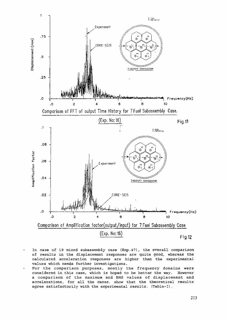
F FJt-3 9E-.ECICP

E

oo5CLv>5

t.O

oÜ

<

.75 -

.5 -

.25 -

Frequ«ncy(ttz).0 2 4 6 8 10

Comparison of FFT of output Time History for 7 Fuel Subassembly Case.

(Exp.No:16)

*••*') Fr«qu«ney(Hz)10

Comparison of Amplification factor(output/input) for 7 Fuel Subossembly Case(Exp. No: 16)

Fig.12

In case of 19 mixed subassetnbly case (Exp.47} , the overall comparisonof results in the displacement responses are quite good, whereas thecalculated acceleration responses are higher than the experimentalvalues which needs further investigations.For the comparison purposes, mostly the frequency domains wereconsidered in this case, which is hoped to be better the way. Howevera comparison of the maximum and RMS values of displacement andaccelerations, for all the cases, show that the theoretical resultsagree satisfactorily with the experimental results. (Table-I).

213

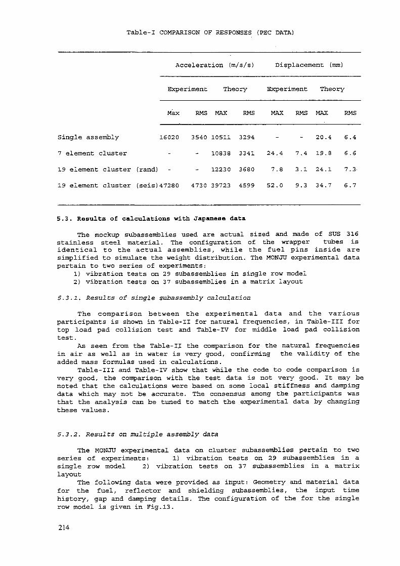
Table-I COMPARISON OF RESPONSES (PEC DATA)

Acceleration (ra/s/s) Displacement (mm)

Experiment Theory Experiment Theory

Max RMS MAX RMS MAX RMS MAX RMS

Single assembly 16020

7

19

19

element

element

element

cluster

cluster (rand)

cluster (seis) 47280

3540 10511

10838

12230

4730 39723

3294

3341

3680

4599

20

24.4 7.4 19

7.8 3.1 24

52.0 9.3 34

.4

.8

.1

.7

6

6

7

6

.4

.6

.3-

.7

5.3. Results of calculations with Japanese data

The mockup subassemblies used are actual sized and made of SUS 316stainless steel material. The configuration of the wrapper tubes isidentical to the actual assemblies, while the fuel pins inside aresimplified to simulate the weight distribution. The MONJU experimental datapertain to two series of experiments :

1) vibration tests on 29 subassemblies in single row model2) vibration tests on 37 subassemblies in a matrix layout

5.3.1. JResults of single subassembly calculation

The comparison between the experimental data and the variousparticipants is shown in Table-II for natural frequencies, in Table-III fortop load pad collision test and Table-IV for middle load pad collisiontest.

As seen from the Table-II the comparison for the natural frequenciesin air as well as in water is very good, confirming the validity of theadded mass formulas used in calculations.

Table-III and Table-IV show that while the code to code comparison isvery good, the comparison with the test data is not very good. It may benoted that the calculations were based on some local stiffness and dampingdata which may not be accurate. The consensus among the participants wasthat the analysis can be tuned to match the experimental data by changingthese values.

5.3.2. .Results on multiple assembly data

The MONJU experimental data on cluster subassemblies pertain to twoseries of experiments: 1) vibration tests on 29 subassemblies in asingle row model 2) vibration tests on 37 subassemblies in a matrixlayout

The following data were provided as input: Geometry and material datafor the fuel, reflector and shielding subassemblies, the input timehistory, gap and damping details. The configuration of the for the singlerow model is given in Fig.13.

214

N/S R/B F/A R/B N/SOOOOOOOOOOOOOOOOOOOOO

FOR T.LP.0.7 mm

FOR M.LP,1.0 mm

F/A : FUEL ASSEMBLYR/B : RADIAL BLANKET ASSEMBLYN/S : NEUTRON SHIELD ASSEMBLY

0.1 mm

Fig. 13 Test Configuration - 29 Assemblies in a Single Row Layout

Table-II COMPARISON OF NATURAL FREQUENCIES

FUEL ASSEMBLYIN AIR IN WATER

BLANKET ASSEMBLY NEUTRON SHIELDIN AIR IN WATER IN AIR IN WATER

EXPT.

BARC, INDIA

IGCAR, INDIA

PNC

HITACHI

MITSUBISHI

TOSHIBA

FRANCE

USSR

3

3

3

3

3

3

3

3

3

.5

.56

.56'

.54

.52

.51

.52

.59

.5

2

2

2

2

3

3

3

3

.9

.85

.83

.92

.09

-

.09

.15

.07

3

3

3

3

3

3

3

3

.3

.35

.61

.33

.33

-

.32

.39 '

.3

2

2

2

2

2

2

2

2

.7

.71

.87

.78

.89

-

.94

.99

.92

2

2

2

2

2

2

2

2

.3

.26

.61

.24

.26

-

.34

.28

.25

2.

1.

2.

2.

2.

-

2.

2.

2.

1

99

30

04

07

17

11

07

215

Table-III COLLISION AT TOP LOAD PADON

EXPT.

IGCAR, INDIA

BARC, IHDIA

PNC

HITACHI

MITSUBISHI

t

FRANCB

MAX. TIME DURATIONFORCEkgf msec msec

5513 0.24 0.70

9866 0.23 '0.52

11000 0.24 0.55

9500 0.24 0.52

10900 0.20 0.60

11223 0.27 0 . 57

15730 ? ?

14566 ? ?

8380 ? 0.85

6850 ? 0.70

SECOND TIME THIRD TIME NODES MODES TIME METHODMAX. MAX. STEPkgf • msec

1500 0.8 1200 1.02

0 - 0 - 13 0.01 DIRECT

0 - 0 - 38 10 0.01 MODAL

0 - 0 - 38 0.01 DIRECT

0 - 0 - 16 0,05 DIRECT

0 - 0 - 15 4 0.005 MODAL

0 - 0 - 2 0 2 ? MODAL

0 - 0 - 20 3 ? MODAL

0 - 0 - 48 3 0.01 MODALNO DAMP

0 - 0 - 48 ' 3 0.01 MODALDAMP

USSR 5614 0 . 50 2500 1800 ? DIRECT

Table-IV COLLISION AT MIDDLE PAD

MAX, TIME HIN TIME SECOND TIME NO OF NO OF TIME METHODFORCE FORCE MAX. NODES MODES STEPkgf msec kg£ msec kgf msec msec

EXPT. 1608 2.50 400 7 .2 720 11,0

IGCAR, INDIA 1195 3.12 343 8 .0 718 12.0 13 0.01 DIRECT

BARC, INDIA 1280 3.20 250 constant at 250 kgffrom 10 to 14 msec

38 10 0.01 MODAL

740 4.00 250 9.0 630 12.5 38 0.01 DIRECT

PNC 1250 3.00 100 constant at 100 kg£ 16 0.05 DIRECT

HITACHI 1395 3.40 235 9.8 504 14.4 15 0.05 MODAL

2127 ? 20 MODAL

MITSUBISHI 1450 ? 200 700 20 MODAL

1210 ? 200 600 48 0.01 MODALNO DAMP

FRANCE 1466 550 600 48 0.01 MODALDAMP

K> USSR 1322 1100 1200 DIRECT

5.3.2.1 Single row test

Seismic calculations were performed for the row configuration with theinput time history corresponding to 0.3 g for the in air calculations and0.4 g for the in water calculations. The shock stiffness value specified attop load pad (TLP) for the subassemblies is equal to 700000 N/mm and so thetime step to be employed for the calculations are very small (of the orderof 1 micro second to 5 micro second) . Usage of such high Ks values incomparison with the Ks values provided by the Italy and France (8600 N/mmand 740 N/mm respectively) has called for very huge solution time (CPU timefor 29 subassembly case, with a time step of 10 micro second, is about 150h in PC 486) . Also for the MONJU data, it was observed, that the use ofsuch high Ks value resulted in some numerical difficulties, which was notobserved when solving the problems with lower Ks values, for example theItalian data and the French data. This is due to the simple spring anddashpot model used in CORE-SETS to express the complex dynamic behaviour ofthe impulse.

The calculations were performed with Ks= 7000 N/mm at TLP and Ks =1200 N/mm at MLP. The results are given in Table-V, Table-VI and Table-VII.

Since the experimental results were given only in the form of plotswithout any digital values, a point to point comparison was not possible. Afew plots for comparison of displacements and strain history for thecentral subassembly are given in the Fig. 14 to Fig.21. It is to be notedhere that the comparison of displacement history as such is not correctbecause the input acceleration used for the calculation is not the measuredacceleration at the shaking table but the input signal to the shakingtable. From the results it can be seen that

generally comparison of the frequency content and the maximum values ofthe displacement and strain time history are good. It is to be notedhere that the comparison of the results in the frequency domain ispreferred rather than the absolute comparison of the responses. Sincedigitized values for the _experimental results were not provided, thecomparison in the frequency domain was not carried out.For in air analysis the difference in displacement values between thetheory and the experiment is within 10 % for the fuel and the reflectorelements. But for the shielding elements the discrepancy is higherbecause in the calculations the Rayleigh damping parameters were tuned

Table-V COMPARISON OF MAXIMUM DISPLACEMENTS (mm) (ROW MODEL)

LocationExpt

In air (0.3 g) In water (0.4 g)

CORE-SEIS Expt CORE-SEIS

DlD2D3D4D5D6D7

11.12.9.9.10.10.10.

,5,5, 0,8,0, 0,0

9'.9.10.10.11.9.9.

91470259026881

1083S8812

.0

.8

.0

.8

.8

.8

.0

11121111111011

.42

.21

.69

.81

.27

.05

.94

218

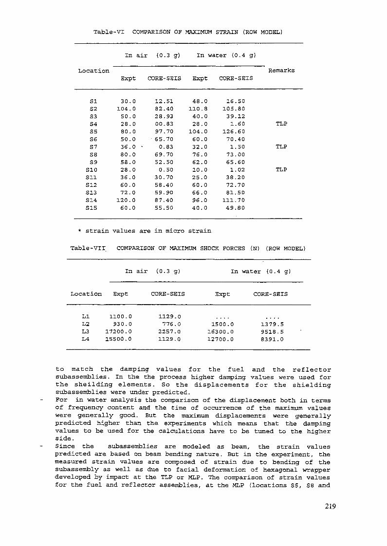
Table-VI COMPARISON OF MAXIMUM STRAIN (ROW MODEL)

In air (0.3 g) In water (0.4 g)

LocationExpt CORE-SEIS Expt CORE-SEIS

Remarks

SIS2S3S4S5S657S3S9S10SllS12S13S14S15

30104502880503680582836607212060

.0

.0

.0

.0

.0

.0

.0 '

.0

.0

.0

.0

.0

.0

.0

.0

1282280097

• 650

69520

3058598755

.51

.40

.93

.83

.70

.70

.83

.70

.50

.50

.70

.40

.90

.40

.50

48110402810460327662102560669640

.0

.8

.0

.0

.0

.0

.0

.0

.0

.0

.0

.0

.0

.0

.0

16105391

12670173651

38728111149

.50

.80

.12

.60

.60

.40

.50

.00

.60

.02

.20

.70

.50

.70

.80

TLP

TLP

TLP

* strain values are in micro strain

Table-Vil COMPARISON OF MAXIMUM SHOCK FORCES (N) (ROW MODEL)

In air (0.3 g) In water (0.4 g)

Location Expt CORE-SEIS Expt CORE-SEIS

LIL2L3L4

1100.0930.0

17200.015500.0

1129.0776.02257.01129.0

1500.016300.012700.0

1379.59518.58391.0

to match the damping values for the fuel and the reflectorsubassemblies. In the the process higher damping values were used forthe sheilding elements. So the displacements for the shieldingsubassemblies were under predicted.For in water analysis the comparison of the displacement both in termsof frequency content and the time of occurrence of the maximum valueswere generally good. But the maximum displacements were generallypredicted higher than the experiments which means that the dampingvalues to be used for the calculations have to be tuned to the higherside.Since the subassemblies are modeled as beam, the strain valuespredicted are based on beam bending nature. But in the experiment, themeasured strain values are composed of strain due to bending of thestibassembly as well as due to facial deformation of hexagonal wrapperdeveloped by impact at the TLP or MLP. The comparison of strain valuesfor the fuel and reflector assemblies, at the MLP (locations S5, S8 and

219

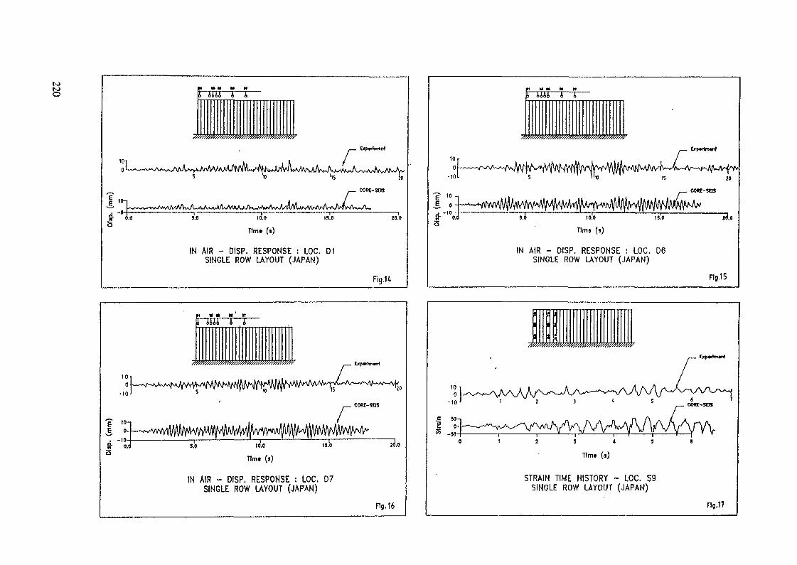
N)K)O

r—•-'~•^AA^/sJAAA^>AM^MA^^^^UY/^^

. -»-r£ 0.0S

5.0 10.0

Tim» (s)

W AIR - DISP. RESPONSE : LOG. 01SINGLE ROW LAYOUT (JAPAN)

codt-sas

Fig.14

Tim« (s)

IN AIR - DISP. RESPONSE : LOG. 06SINGLE ROW LAYOUT (JAPAN)

Flg.15

M • M W

IN AIR - DISP. RESPONSE : LOG. 07SINGLE ROW LAYOUT (JAPAN)

Flg. 16

Tlmt (s)

STRAIN TIME HISTORY - LOG. S9SINGLE ROW LAYOUT (JAPAN)

Flg.17

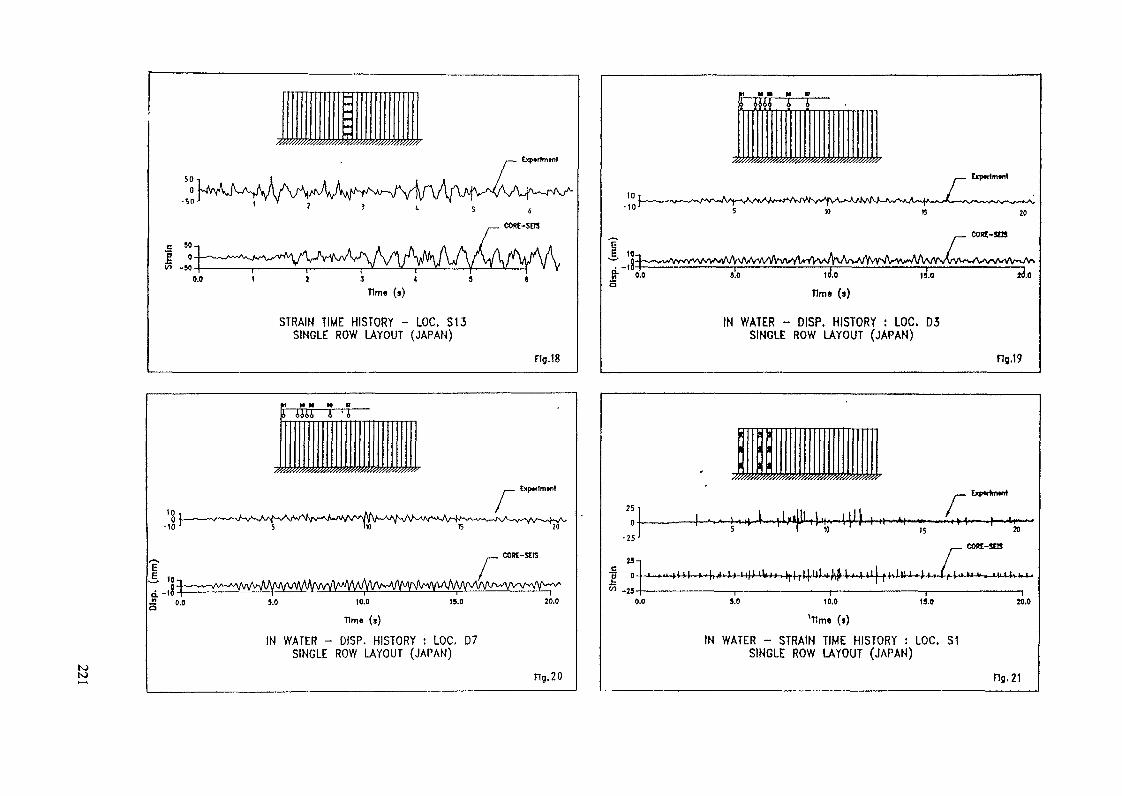
Tim» (s)

STRAIN TIME HISTORY - LOC. SI3SINGLE ROW LAYOUT (JAPAN)

Exp*r1m»nf

F1g.18

IN WATER - DISP. HISTORY : LOC. D3SINGLE ROW LAYOUT (JAPAN)

Ftg.19

*1 H H HI

j> AiAA À •V

&

Tim« (s)

IN WATER - DISP. HISTORY : LOC. D7SINGLE ROW LAYOUT (JAPAN)

COB£-S£1S

20.0

Hg.20

1 ! 1

1 1 1

1 1 1

25 ..

-2S

£ Tl, Ki t r H J , ' , f * „ tfn -,,

-r JH— -jJ -H*- * -* ——— '•H —— H — —10 r 15 JO

— cws-sns

|,!lt, )^ !,,,.< ki, f (,h|.i -J.i , \f u-.»' «*. JuiUhi.2 3 l i 1 1 1

0,0 3.0 10.0 tS.O ÏO.O

lT1m» (»)

IN WATER - STRAIN TIME HISTORY : LOC. S1SINGLE ROW LAYOUT (JAPAN)

ns.21

S12) and at the foot (locations S6, S9 and S15) are within 20 %. Thepredicted strain values at TLP are very small which is in accordancewith the classical theory that the strain at the cantilever tip due tobase motion is almost nil.The acceleration responses were high of the order of 30-50g, which isof the same order as obtained in the analysis of Italian data.From the results one can see that the global behaviour of thesubassembly is unaffected by the use of lower Ks values. The use oflower Ks values in the calculations has affected the results such as(i) the shock force at the TLP (ii) the acceleration values.

5.3.2.2 Cluster test

Due to limitation in the time available, only the central row with 7sub assemblies was analysed. It has been observed from the results of theanalysis of the Italian data, that such central row analysis gives equallygood results as the cluster analysis. For this analysis also ,As discussedin 4.2, reduced Ks value was used. The Table-VIII, Table-IX and Table-Xgive the comparison of the calculated maximum response values fordisplacement, strain and shock force. From the Tables one can see that

The difference in the displacement between the experiments and thecalculations is around 10 %, except at the location D3 (in water) . Atthe location D3 the calculated maximum- displacement values seems to beof the same order as the adjacent subassemblies, The reason for the lowexperimentally observed values is not known.The comparison of strain values at the MLP and at the foot are good(within 20 %) . At the TLP the strain values are low.

Table-VIII COMPARISON OF MAX. DISPLACEMENTS (mm) (CLUSTER MODEL)

In air In water

Location Expt CORE-SEIS Expt CORE-SEIS

DlD2D3D4

4.504.753.203.50

5.275.044.473.58

5.205.252.103.70

6.125.864.944.14

The following are the important conclusions :

The displacement and strain values are generally predicted well. Thedifference in displacement values between the theory and the experimentis about 10 % for the 'In 'air' calculations and about 20 % for the 'inwater' calculations.The strain values at MLP and at the foot of the subassembly comparewell within 20 %. The strain value at TLP is low, which is inaccordance with the classical theory. The reason for the lowerexperimentally observed value has to be studied.A shock stiffness value of 7000 N/mm at TLP is used in the calculationsinstead of 7E5 N/mm. The use of lower KS value has affected theresults such as (i) shock force (ii) the acceleration values.

222

Table-IX COMPARISON OF MAXIMUM STRAIN (CLUSTER MODEL)

LocationIn air (0.3 g) In water (0.4 g)

Remarks

Expt CORE-SEIS Expt CORE-SEIS

SIS2S3S4S5S6S7

40.82.17.33.69.27.35.

0555007

37650

36670

38

.7

.7

.6

.6

.3

.7

.5

29611732697

36

.0

.5

.5

.5

.2

.5

.7

41.79.1.43.88.1.47.

7330737

TLP

TLP

* strain values are in micro strain

Table-X COMPARISON OP MAX. SHOCK FORCES (N) (CLUSTER MODEL)

In air In water

Location Expt CORE-SEIS Expt CORE-SEIS

LIL2

2500.012500.0

358.01853.0

600.08500.0

477.03006.0

6. RECOMMENDATIONS FOR FURTHER STUDIES

The seismic response has got direct bearing on the reactivityoscillations of the core. The seismic vertical and horizontal oscillationsof the rector core can lead to reactivity changes due to control rodoscillations in the core, core compaction etc.. The core seismic analysisis complete only with the evaluation of such neutronic seismicinteraction effects and computing the final reactivity oscillations due tothe seismic event. The complexity of these calculations is well recognisedand it is imperative that such calculations are to be verified andvalidated with proper experimental data. Towards this it is recommendedthat the present CRP can be extended to include these core seismicreactivity oscillation calculations.

7. CONCLUSIONS

Towards the IAEA/IWGFR CRP on 'Intercomparison of LMFBR core seismiccodes', calculations have been performed for the RAPSODIE core mockup datasupplied by France, PEC data supplied by Italy and MONJU core mockup datasupplied by Japan, using the computer code CORE-SEIS developed by IGCAR,KALPAKKAM, INDIA. The following are the important conclusions:

223

French data

The predicted natural frequency of the fuel sub assembly by lineareigen value analysis is 8.14 Hz and by non-linear time history analysisis 7.6 Hz which compares very well with the experimentally observedvalue of 8.0 Hz.The seismic calculations were performed on the central row of the subassembly. The comparison of tip displacement history for fuel subassembly is good both in terms of the frequency content and magnitude.For shielding sub assemblies the difference is high due to higherdamping value used in the calculations because the Rayleigh dampingparameters were adjusted for the fuel subassemblies.

Italian data

For the configuration with the identical subassemblies, the analysiswith single assembly gives satisfactory responses under random baseexcitations. Thus, it implies that the possible variations in thesupporting conditions at the foot are not critical for responsecalculations.In case of 19 mixed subassembly case (Exp.47), the overall comparisonof results in the displacement responses are quite good, whereas thecalculated acceleration responses are higher than the experimentalvalues which needs further investigations.Comparison of the maximum and RMS values of displacement andaccelerations, for all the cases, show that the theoretical resultsagree satisfactorily with the experimental results.

Japanese data

The displacement and strain values are generally predicted well. Thedifference in displacement values between the theory and the experimentis about 10 % for the 'In air' calculations and about 20 % for the 'inwater' calculations.The strain values at MLP and at the foot of the subassembly comparewell within 20 %. The strain value at TLP is low, which is inaccordance with the classical theory. The reason for the lowerexperimentally observed value has to be studied.Since the use large Ks value such as 7E5 N/mm resulted in calculationinstabilities, a shock stiffness value of 7000 N/mm at TLP is used inthe calculations. The use of lower KS value has affected the resultssuch as (i) shock force (ii) the acceleration values.

REFERENCES

[1] BROCHARD, D., P.BULAND, F.GANTENBEIN and R.J.GIBERT (1987), "Seismicanalysis of LMFBR core. Mock Up RAPSODIE", Proc. Ninth Int. Conf. onStructural Mechanics in Reactor Technology, Laussane, Vol.E, pp.33-42.

[2] HORIUCHI, T., M.NAKAGAWA and H.KASAI (1993), "Development of SAFA, Aseismic analysis program for FBR core components", Proc. 12th Int.Conf. on Structural Mechanics in Reactor Technology, Stuttgart, Vol.E,Paper.E13/2, pp.381-386.

[3] MARTELLI, A., M.FORNI, P.MASONI, G.MARESCA, A.CASTOLDI, F.MUZZI (1988),"Research and development studies on plant and core seismic behaviourfor fast reactor", Nuclear engineering and design, Vol.106, pp.103-126.

224

[4] MORICHITA, M. and K. IWATA (1993) , "Seismic behaviour of free standingcore in a large LMFBR", Nuclear engineering and design, Vol.140,pp.309-318

[5] RAVI,R., VAZE,K.K.,BHOJE,S.B, " Seismic analysis of reactorassembly" ,Proc. 10th Int. Conf. on Structural Mechanics in ReactorTechnology, Vol.K, pp.139-144

[6] RAVI,R., ATHIANNAN,K., SELVARAJ,T., CHELLAPANDI,P., BHOJE,S.B, "Theoretical and experimental investigations of seismic behaviour ofreactor assembly of PFBR",Proc. llth Int. Conf. on Structural Mechanicsin Reactor Technology, Vol.E, pp.449-454

Next page(s) left blank 225

ANALYSIS OF THE CORE SEISMIC EXPERIMENTSUSING THE COSMOS/M CODE

K.K. VAZE, B. MURLIReactor Engineering Division,Bhabha Atomic Research Centre,Trombay, Bombay,India

Abstract

In a typical Liquid Metal Fast Breeder Reactor (LMFBR) the fuel pins are contained inhexagonal assemblies which rest on the diagrid. In a cluster of assemblies, there is a possibiityof contact between the neighbouring assemblies at the pad level during a seismic event. Thedeflected core may have more reactivity due to core compaction. Therefore, core seismicanalysis is an important item to ensure fast reactor safety in an earthquake.

Numerous experiments have been conducted in different countries on single assembly, a row ofassemblies and on small and large clusters. In order to enhance the quality and extent ofvalidation of the codes it was of interest to analyse the data using different codes.

Under the Co-ordinated Research Program on 'Inter comparison of LMFBR Seismic AnalysisCodes' analyses have been performed for the following tests.

Italy - Shake table testing of 7 and 19 element clusters.Japan - Natural frequency and impact tests on single assembly in air and waterJapan - Shake table testing of 29 element row and 37 element clusterFrance - — do - Rapsodie core mock-up.

The calculated results were compared with experimental data in respect of- maximum and RMS displacement and acceleration of a particular assembly- Fourier Spectra of displacement and acceleration.

It was found that the displacement responses; matched very well but there was a discrepancy inthe acceleration. The possible causes of this are i) imprecise determination of shockparameters ii) Filtering of high frequency acceleration signal in experimental measurements.

Due to the limitations of the computer program, the large cluster problem (Rapsodie mock-up)could not be solved. Apart from this, no other major limitation of the code was identified. It wasconcluded that the code has been validated against experimental data. Apart from this, theparticipants have also derived immense benefit in the areas of modelling of gaps, damping, fluideffects, measurements and processing of data.

1.0 SUMMARY:

Worldover, the design of the core of the Liquid Metal Fast BreederReactor (LMFBR) is found to have many similarities. The fuel elements in theform of pins are contained in hexagonal assemblies (wrappers). Theseassemblies rest on the diagrid and in many designs are of free-standing type;i.e., there is no external restraint against their radial movement (bowing). Theinternal restraint is derived from the fact that the clearances between theassemblies are very much reduced by providing pads (buttons) at one or twolocations along the height. The fuel assemblies are surrounded by the reflector,blanket and shielding assemblies.

227

During a seismic event, the seismic motion is transmitted to theassemblies through the diagrid. The resultant deflection of a single assembly isgoverned by its natural frequency (reduced due presence of liquid sodium),damping and the frequency content of the seismic motion at the diagrid level (thefloor response spectrum).

However, in a cluster of assemnblies, there is a possibiity of contactbetween the neighbouring assemnblies at the pad level. This limits thedeflections but intoduces impact forces of short duration. There is a possibilitythat the deflected core has more reactivity due to core compaction. Therefore,core seismic analysis is an important item to ensure fast reactor safety in anearthquake.

Various computer codes have been developed in different countries fornon-linear seismic analysis of LMFBR core. In addition, numerous experimenthave been conducted on single assembly, a row of assemblies and on small andlarge clusters. In order to enhance the quality and extent of validation of thecodes it was of interest to analyse the data available in different countries usingdifferent codes.

With this objective in mind, the Co-ordinated Research Program on'Inter comparison of LMFBR Seismic Analysis Codes' was started with the firstconsultancy meeting held in Oct. 1990. Over a period of four years, theparticipadnts have performed analyses for the following tests.

Test data TestSupplied by

Japan - Natural frequency determination of single assembly in air andwater.

Japan - Impact of single assembly on rigid mass.Italy - Shake table testing of 7 element cluster.

„ - -do- 19 -do- (allfuel)- do - 19 - do- (fuel + reflectror)

Japan - — do — 29 element rowJapan - — do — 37 element clusterFrance - — do — Rapsodie mock-up core.

This report gives the details of the calculations performed at BhabhaAtomioc Research Center. India. After giving the features of the computer codeused and describing the modelling aspects the report gives the results of thecalculations and the comparison with experimental data.

The comparison is made with respect to -

- maximum displacement of a particular assembly- R.M.S displacement of a particular assembly- maximum acceleration of a particular assembly- R.M.S acceleration of a particular assembly- Fourier Spectra of displacement and acceleration.

228

It was found that the displacement responses; both (maximum andRMS) matched very well but there was a discrepancy in the acceleration,particularly the maximum acceleration. Since this discrepancy was observed byall the prticipants it is perhaps due to imprecise determination of shockparameters.

Due to the limitations of the computer program, the large clusterproblem (Rapsodie mock-up) could not be solved.

Apart from this, no other major limitation of the code was identified. Itwas concluded that the code has been validated against experimental data.Apart from this, the participants have also derived immense benefit in the areasof modelling of gaps, damping, fluid effects, measurements and processing ofdata.

As future extension of the program the following suggestios aremade.

- Its forward integration into a reactivity calculation program.- Its backward integration into a code for seismic analysis of reactor

block. Since the seismic motion of diagrid is an input to the coreanalysis it needs to be put on a firm footing by validating themodelling aspects and the codes which perform these calculations.

2.0 REVIEW OF SEISMIC ANALYSIS WORK

- Seismic analysis work in Bhabha Atomic Research Centre is carried out insupport of 235 MWe and 500 MWe Pressurised Heavy Water Reactors(PHWRs). The Reactor Building of these reactors is a complex structureconsisting of Inner and Outer Containment Buildings, Internal Structure andCalandria Vault. For the purpose of calculating the forces and moments invarious members of this structure and for evaluating the floor response spectra,a stick model is employed. The beam properties of these complex cross-sectionsare not amenable to simple calculation. A procedure based on strain energyequivalence was developed for evaluating these properties. A paper publishedon this work is enclosed as Annexure I.

- The methodolgy developed for nonlinear analysis of LMFBR Cores caneasily be applied to nonlinear analysis of piping involving gap supports.Annexure II describes the exercise performed for validating the code for such ananalysis using a benchmark problem available in literature.

- In the seismic analysis of nuclear reactor buildings, the evaluation ofseismic response and ultimate strength is important in verifying the reliability ofequipment and components. The evaluation of the ultimate strength is also animportant issue when assessing the seismic safety factor of buildings. TheNuclear Power Engineering Corporation (NUPEC) of Japan has conducted aproject entitled "Elastoplastic Test of Reactor Buildings". As part of this project,the "Seismic Ultimate Dynamic Response Test" was carried out using a large-

229

scale, high performance shaking table at NUPEC's Tadotsu EngineeringLaboratory in 1991. The dynamic response behaviour of RC shear walls wasstudied and test data, useful for verification of seismic analysis codes, wereobtained. NUPEC has offered the utilization of this data as a Seismic ShearWall International Standard Problem (SSWISP), sponsored byOECD/NEA/CSNI. Bhabha Atomic Research Centre is also participating in thisvalidation exercise. The test was conducted in five stages with increasing levelsof amplitude, finally leading to collapse. Calculations for the first two stages havebeen completed and further calculations are in progress.

3.0 DESCRIPTION OF COMPUTER CODE

COSMOS/M:

Cosmos/M is a complete, modular, self-contained finite elementsystem developed by Structural Research and Analysis Corporation forpersonal computers and work stations. The program includes modules tosolve linear and nonlinear, static and dynamic structural problems.

The Cosmos/M system consists of a pre- and post processor,various analysis modules, interfaces, translators and utilities.

Frequency Analysis Module:

This module evaluates natural frequencies and the correspondingmode shapes of a system. The following are some important features:

. Eigenvalue extraction methods:- Subspace iteration- Lanczos- Jacobi- Inverse power iteration- Cyan Reduction

Advanced Dynamic Analysis Module:

This module uses the normal mode superposition methos tocalculate dynamic response of structures. The following are some importantfeatures:

. Analysis options:- Modal time history- Uniform and Multi-base motion- frequency response- shock spectra- Response spectra generation- Random vibration- Steady-state harmonic analysis- PSD/Random response

230

. Damping models- Scalar- Dashpot- Discrete viscous- Modal viscous- Structural- Material

. Initial conditions

. Time and frequency curves

. Stress analysis

. 2-node gap element problems with friction

Finite Element:

A breif description of the finite element used to model the LMFBRcore sub-assemblies namely the 3-D beam element is given below.

1) BEAM3D is a 2-node uniaxial element for three-dimensionalstructural models. For structural analysis, six(6) degrees of freedom (threetranslations and three rotations) are considered per node. This elementpermits using the unsymmetric cross-section when the shear center is notcoincident with the center of gravity; e.g., channel and L-shape cross-sections can be considered.

Forces,moments,and stresses are available in the elementcoordinate system.

2) The GAP element is defined by two nodes representing thedistance between any two points in a two- or three-dinensional model. Theactual gap separation is defined independent of the node locations and canassume any value including the distance between the modes. The elementresists either compression or tension depending on whether the gap distanceis positive or negative. An iterative procedure is adopted in the solution ofproblems involving gap elements. The iteration is performed at the end ofeach time step on gap elements closed, to ensure convergence of the forcein the element to its correct value corresponding to the relative displacementbetween the two nodes.

231

4.0 PROBLEMS & RESULTS

4.1 FREE VIBRATION TEST ON SINGLE ASSEMBLY

4.1.1 Problem Definition

Defined by: Dr. K. IwataPower Reactor and Nuclear Fuel DevelopmentCorporationJAPAN

Experiments conducted at : JAPAN

Three kinds of core sub-assembly models, namely,

i) Core Fuel Assemblyii) Radial Blanket Assembly and

iii) Neutron Shield Assembly

were tested by giving them an initial displacement of 10 mm at the top.Natural requencies were measured both in air and in water. See figure 4.1 forthe schematic of the test setup.

5: initiai Displacement( 10 RIB )

(A) Test Assembly(B) Support Plate(C) Tank

* In Air • In Hater

Fig. 4.1 Schematic View of Free Vibration Test

232

4.1.2 Input Data

The mass and stiffness datas were supplied by the experimenters.The datas required for modelling the sub-assemblies are provided in tables4.1 to 4.3.

4.1.3 Analysis

4.1.3.1 Natural Frequency Analysis

4.1.3.1 a. Free Vibrations in Air

The analyses were carried out using the general purpose finite elementcomputer code COSMOS/M. Two kinds of analyses were carried out.

(i) Linear Eigenvalue Analysis

The boundary conditions used for this analysis were pinned supports atthe upper and the lower support plates.

(ii) Nonlinear Time History Analysis

The boundary conditions were modified as follows. At both, upper andlower support plates, a gap support condition was simulated by adding gapelements on either side of the nodes at these locations. The gap distance wasset to 0.1 mm equal to the clearance avaible.

The assembly was given an initial displacement of 10 mm at the top byimposing a corresponding force. This force was then released suddenly and anonlinear time history analysis was carried out by direct integration methodwith a time step of 0.01 msec.

4.1.3.1b Free Vibrations in Water

Only the linear eigenvalue analysis was performed for this case. Thefinite element model used was same, but the densities were modified toaccount for the added mass due to water. The added mass was calculated asfollows.

(i) Added Mass due to Water Outside

This was assumed equal to the mass of water contained in a cylinderwith diameter equal to the corner-to-corner distance of the envelopinghexagon. The mass was calculated for individual sections which have differenthexagonal dimensions.

233

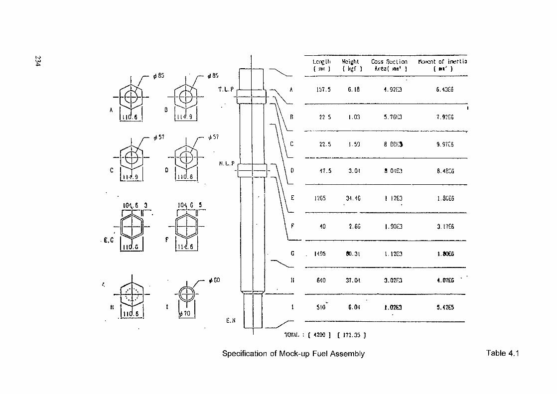
Lcnglli Height Cous Suction fluent of inert ia( um ) ( t<uf } Area( mn1 ) ( m' )

Ib7 .5 6.18

22.5 1.50

1205

1405 80.31

l 510 G.O'I

10FAI, : ( 4200 ] [ 172.35 ]

Specification of Mock-up Fuel Assembly

22 5 1.03 5.7GI-3

8 B8I3

17.5 3.0-1 8 O'i

I I2E3

2. GO 1.9013

I .12E3

II 640 37.0-1 3.02Ü

I.02Q

6. «Go

7.92EG

9.97C5

8.4SCÔ

3.I7C6

i.soec

4.07EG

5.42E5

Table 4.1

IO-\.C 3JPBT

110 .G

.G

[ci\i\.}\ Hci j j l i l Cuss Scclioo ftjncnt Of inenia( »'" ) ( kgf ) A i c o ( mn' ) ( mn1 )-

157.5 G. 18 ' 4.92E3

22.5 1.03

•17.5 3.0-1

12G5 3-1.98

510 6.0-1

5.7GE3

1.59 8.88E3

8.0-1E3

1.I2D

3.12 J.90E3

H95 98 32 I .12E3

C-IO ' 37.79 2.25E3

1.02E3

TOTAt, : ( -1200 ] [ 192.00 ]

6.43EG

7.92EG

8.18EC

I.80EB

3.17EO

1.80EG

2.98E6

5.42E5

Specification of mock-up Radial Blanket Assembly Table 4.2

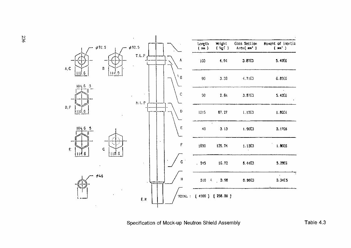
to

092 .5

A.CIII/ .6

r 092.5

T.L.I'

.9

i). Fid. l

10'V G 5v-,,

l l-f.8

-L-

M.L.P

F.. H

A

Ü

C

D

i——,

f

r — •

C '

r—

II

i —

Length( m« )

1GO

90

50

1215

40

1890

. 2-15

510 ••

Height Coss Section( kgf ) Arca{ «•' )

4.9-1 3.87E3

3.33 4.71E3

2.8-1 3.87E3

87.27 I.I2FJ

3.13 1.90E3

1.15.74 1.1 2G3

IG. 72 6.44Ë3

3.93 0.98E3

ftancnt of inertia

5.40EG

G.891ZG

5.40E6

1.8CE6

3.17E6

I.80C6

5.29EG

3.3-1E5

TOPAL : [ 4200 J [ 258.00 ]

Specification of Mock-up Neutron Shield Assembly Table 4.3

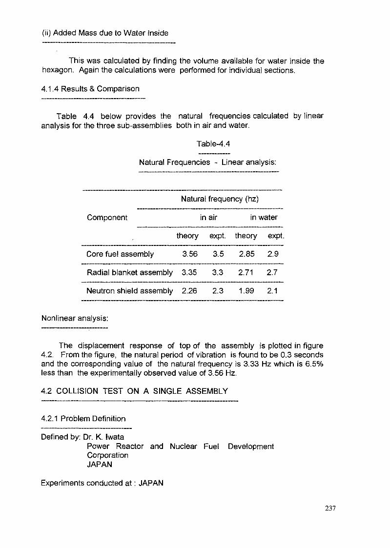
(ii) Added Mass due to Water Inside

This was calculated by finding the volume available for water inside thehexagon. Again the calculations were performed for individual sections.

4.1.4 Results & Comparison

Table 4.4 below provides the natural frequencies calculated by linearanalysis for the three sub-assemblies both in air and water.

Table-4.4

Natural Frequencies - Linear analysis:

Natural frequency (hz)

Component in air in water

theory expt. theory expt.

Core fuel assembly 3.56 3.5 2.85 2.9

Radial blanket assembly 3.35 3.3 2.71 2.7

Neutron shield assembly 2.26 2.3 1.99 2.1

Nonlinear analysis:

The displacement response of top of the assembly is plotted in figure4.2. From the figure, the natural period of vibration is found to be 0.3 secondsand the corresponding value of the natural frequency is 3.33 Hz which is 6.5%less than the experimentally observed value of 3.56 Hz.

4.2 COLLISION TEST ON A SINGLE ASSEMBLY

4.2.1 Problem Definition

Defined by: Dr. K. IwataPower Reactor and Nuclear Fuel DevelopmentCorporationJAPAN

Experiments conducted at : JAPAN

237

1 5E-002

1 OE-002

5 OE-003

0 OE+000CDE0)

-5 OE-003

COQ

-1 OE-002

-1 5E-002

-2 OE-002

\

00 02 03 04 05 06Time in seconds

07 08 09 1 0

Figure 4.2Frequency calculation by Nonlinear Analysis

The assembly model is given an initial displacement of 50 mm at the topload pad and is released to collide with a heavy weight at the top load pad(TLP) or at the Middle Load Pad (MLP). Collision forces were measured withthe load cell on the heavy mass. See figure 4.3 for the schematic of the testsetup.

4.2.2 Input Data

The mass and stiffness datas were supplied by the experimenters.The datas required for modelling the sub-assemblies are provided in tables4.1 to 4.3.

4.2.3 Analysis

Collision Test on Single Assembly

The model used for this analysis was same as the one used earlier fornonlinear time history analysis i.e. gap elements at the upper and lowersupport plates with gap distance = 0.1 mm were used. In addition, anothergap element was introduced at the top load pad (TLP) or the middle load pad(MLP) depending on the location of the collision. The gap distance for thiselement was set to zero, and the gap stiffnesses were set equal to the localstiffness of the load pads i.e.

238

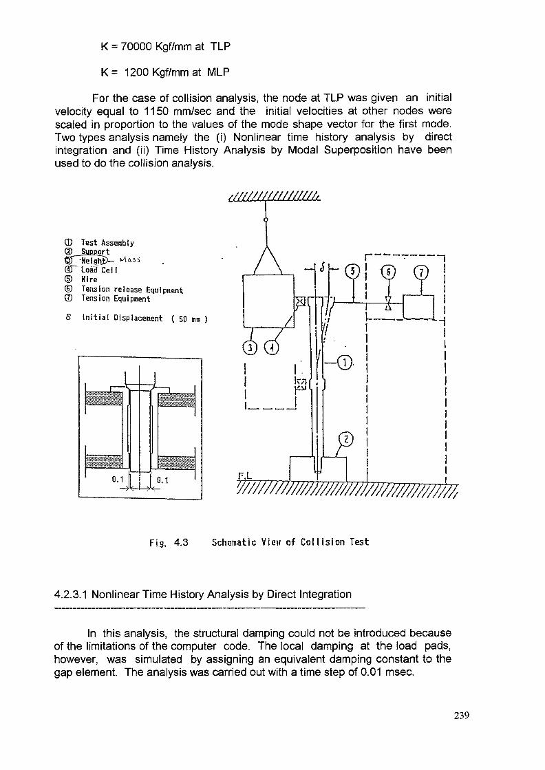
K = 70000 Kgf/mm at TIP

K= 1200 Kgf/mm at MLP

For the case of collision analysis, the node at TLP was given an initialvelocity equal to 1150 mm/sec and the initial velocities at other nodes werescaled in proportion to the values of the mode shape vector for the first mode.Two types analysis namely the (i) Nonlinear time history analysis by directintegration and (ii) Time History Analysis by Modal Superposition have beenused to do the collision analysis.

(D Test Assembly

® "Load" Cell© Hire© Tension release Equipment® Tension EquipmentS Initial Displacement ( 50 mm )

0.1Wf/lX,mm/.

0.1

Fig, 4.3 Schematic V iew of Col l is ion Test

4.2.3.1 Nonlinear Time History Analysis by Direct Integration

In this analysis, the structural damping could not be introduced becauseof the limitations of the computer code. The local damping at the load pads,however, was simulated by assigning an equivalent damping constant to thegap element. The analysis was carried out with a time step of 0.01 msec.

239

4.2.3.2 Time History Analysis by Modal Superposition

The first phase in this analysis consists of finding the naturalfrequencies and mode shapes. For this purpose, the boundary conditions atthe upper and lower support plates were changed. The translation degrees offreedom of the nodes at these locations are not constrained. The rotationdegree of freedom at the bottom most node was constrained. Thus, a rigidmode corresponding to the translation is included in the analysis.

The frequency and mode shape data calculated in the first phase areused in a modal superposition analysis with 10 modes included.

Structural damping was introduced by assuming that the damping matrixis of the form

[C] = a * [ M ] + b * [ K ]

The constants ' a ' and ' b ' were adjusted so as to give 3% dampingfor the first mode ( f1 = 3.56 Hz ) and 15% damping for the second mode ( f2 =19.1 Hz).

The local damping at the load pads was also simulated using a damperelement across the gap. The damping constant was adjusted to give a dampingcoefficient of 11 %.

4.2.4 Results & Comparison

Nonlinear Time History Analysis by Direct Integration

The results of these analyses are shown in

fig 4.4 for collision at TLP,

fig 4.5 for collision at MLP

The experimental values are also plotted in the same figures. Thesignificant findings like peak force and the time at which the peak force occursare shown in table 4.5.

Time History Analysis by Modal Superposition

The results of these analyses are shown in

fig 4.6 for collision at TLP,

fig 4.7 for collision at MLP

240

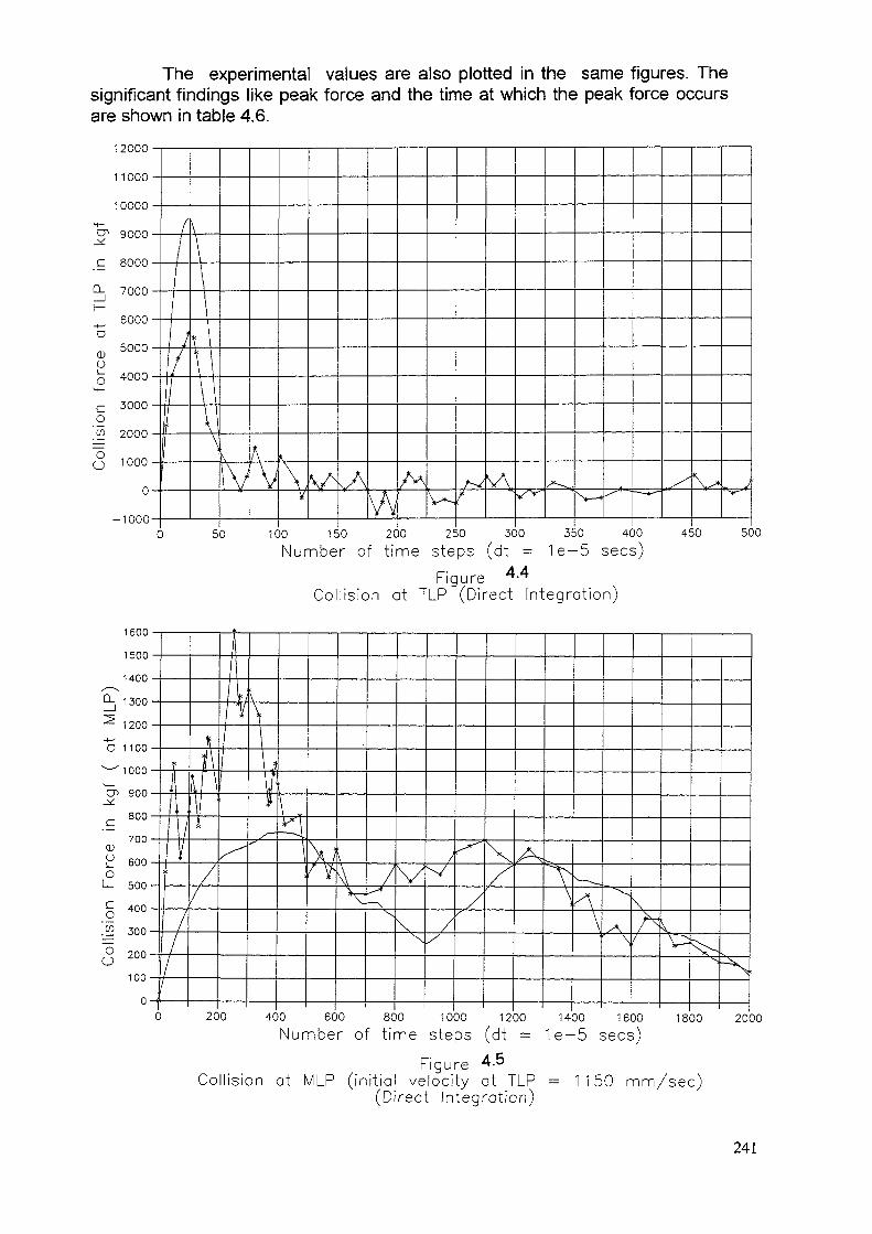
The experimental values are also plotted in the same figures. Thesignificant findings like peak force and the time at which the peak force occursare shown in table 4.6.

12000'11000 •10000 •9000 •8000-

7000 •

6000 •

(Uo5000-

4000-

c 3000•O'w 2000-

O 1000-

-1000-v*-,

100 150 200 250 300 350 400 450Number of time steps (dt = 1e-5 sees)

Figure ^.4Collision at TLP (Direct Integration)

500

a.

en

c

1600 •1500 -1400 -1300 •1200 •1100-'1000-

900-800-700-600-500-400-

oL_OL_CO.52 300-OO 200-

100-

200 400 600 800 1000 1200 1400 1600 1800Number of time steps (dt = 1e-5 sees)

Figure 4.5Collision at MLP (initial velocity at TLP = 1150 mm/sec)

(Direct Integration)

2000

241

(O

O O_ Öj' o'

T)

o CL c c "D CD '

—l ~D O — 5' D

tt>_1 O

CD

Cn O 3 3 0) 0) o

-1 o-

Z °

C c^S

.

3 CD

~;

W CD

o~O CL

o'

o

CD

_>l

•*"l

o-

cn o

03 CDO

)O

"• o oo O

"o to o O

"o

Col

lisio

n Fo

rce

in

kgf

( at

M

LP)

-i

NJ

OJ

-

Ul

O)

O

O

O

O

O

Oo

o

o

o

o

o

o

\

o o_ W 0'

Q ~oi] 03

"O o CO rt-" o' D

Col

lisio

n fo

rce

at

TLP

in

kgf

o o oo o o

M O O O

o o oo o o

en o o o

Öl o o o

o o o

oo o o o

CD o o o

o o o oo o o

o-

o

O"

g"O er.

N>

-,

o-

CD COO Q

. -•'^"

s:.

'-t-co

o>c "a CD

CD-

CD ,l

&-|

CO CD o

^VI

O

-v,_

^- O cn

-o

Table 4.5

Collision at TLP

Expt Analysis by Analysis bydirect integration Modal Superposition

Peak Force 5513 9500 11000Kgf

Time ofoccurrence 0.24 0.24 0.24(msec)

Table 4.6

Collision at MLP

Expt. Analysis by Analysis bydirect integration Modal Superposition

Peak Force 1608 740 1280Kgf

Time ofoccurrence 2.5 4.0 3.2(msec)

4.3 PEC CORE MOCK UP TESTS

4.3.1 Problem Definition

Defined by: Dr. Martelli

experiments conducted at: ITALY

This problem consists of the following cases.

i) Single fuel element in water subjected to 0 db excitation, Time historyNo. 3, Tape 1

ii) A cluster of 7 fuel elements in water, 0 db excitation, Time history No. 7,Tape 1

iii) A cluster of 19 fuel elements in water, 0 db excitation, Time history No.11, Tape 1 .

243

iv) A cluster of 8 fuel and 11 reflecting elements in water, 0 db excitation,Time history No. 61 of Tape 3

Analysis of Single fuel element in water subjected to 0 db excitation.

4.3.2 Input Data

4.3.2.1 Geometrical Details

The core of the Italian fast reactor PEC consists of hexagonal shroudswith flat-to-flat distance of 82.6 mm in cold condition. The elements receivesupport through the foot sections called spikes, which are inserted in the canlike diagrid structure. Two sets of pads are fitted to the core elements; one atthe element midplane and the other at 2.6 m from element base; to reduceinternal clearances and thus, element seismic relative motions to very smallvalues. This limits neutronic-seismic interactions to an acceptable level.

The mock-up elements are prototype hexagonal shroudsreproducing the geometry of the fuel and reflecting elements. The spikes arecylindrical, with two contact spheres which simulate the actual spike-canclearances. (Fig 4.8). The weights of the elements were obtained by filling theshrouds with a mixer of silicone rubber and lead shots. This avoids thepresence of internal non-linearities. Thus, the fuel and the reflectingelements differ only in the weights given by the different densities of theinner materials.

The fuel and reflecting elements are separated from each otherthrough small clearances ( gaps ) at the pad locations. The values of theclearances at the top and middle pads are given in Table-4.7. The locationsAO, A1 etc. are shown in Fig 4.9.

4.3.2.2 Stiffness Properties

Beam Properties

The hexagonal elements are modelled as beams. The stiffnessproperties of the beams representing the fuel elements viz. cross-sectionalarea and moment of inertia are given in Table-4.8. The stiffness properties ofthe reflecting elements are identical.

Shock Stiffness

When the elements strike each other at the pad locations during theseismic motion, there is a local deformation of the faces of the hexagons. Thestiffness associated with this is termed as shock stiffness. This is evaluated byconducting tests on the elements, in which, the force and the deformation aremeasured. (Fig 4.10). The stiffness values at the two pad locations are givenin Table-4.7.

244 .

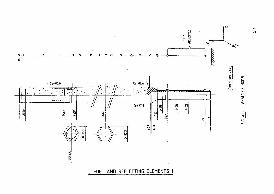
QLU (Nl/J

U4 0

• 3A

•<*-£* ————— o ———————— « — e —— o —— o — e — <3> —— © —— e —— e —— © — e —— e —— -Q _

*-

irr»«I

oo

•»

(UCM

ni/)oistLU

S

QO

1/5

CO

LD

( FUEL AND REFLECTING ELEMENTS )

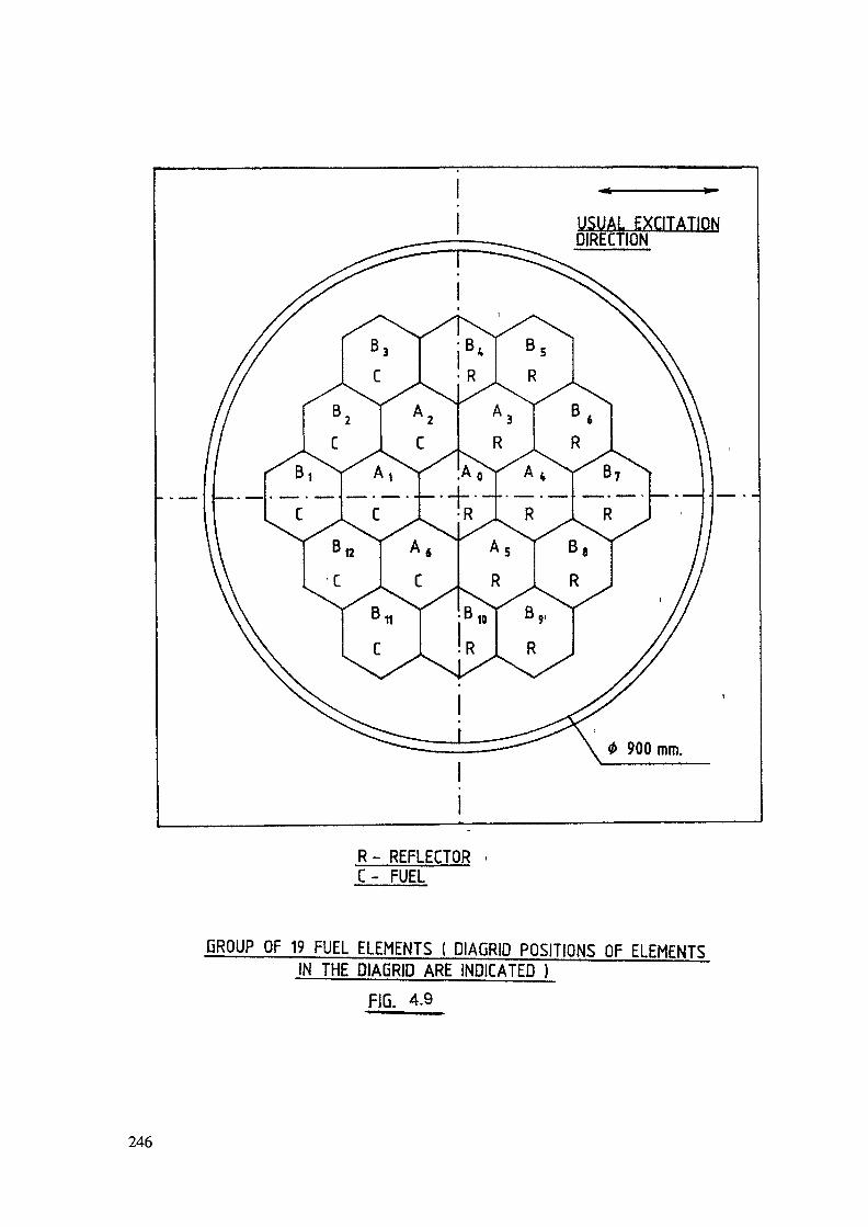
USUAL EXCITATIONDIRECTION

R - REFLECTOR .C- FUEL

GROUP OF 19 FUEL ELEMENTS ( DIAGRID POSITIONS OF ELEMENTSIN THE DIAGRID ARE INDICATED )

FIG. 4.9

246

Table 4.7

Gap and Shock Parameters

Adjacentelements

AO-A1AO-A2AO-A3AO-A4AO-A5AO-A6A1-A6A1-A2A1-A6A1-B1A1-B12A2-A3A2-B2A2-B3A2-B4A3-A4A3-B4A3-B5A3-B6A4-A5A4-B6,A4-B7A4-B8A5-A6A5-B8A5-B9A5-B10A6-B10A6-B11A6-B12B1-B2B1-B12B2-B3B3-B4B4-B5B5-B6B6-B7B11-B8B8-B9B9-B10B10-B11B11-B12

Gap atMLPcm

0.0250.0500.0500.0250.0500.0500.0500.0500.1150.1860.1860.0260.0920.2300.1860.0500.1860.2300.0920.0500.1860.1150.1860.0260.0920.2300.1860.1860.2300.0920.1400.1400.1400.0700.0700.1400.1400.1400.1400.0700.0700.140

Gap atTLP

cm

0.0250.0500.0500.0250.0500.0500.0500.0500.1150.1860.1860.0260.0920.2300.1860.0500.1860.2300.0920.0500.1860.1150.1860.0260.0920.2300.1860.1860.2300.0920.1400.1400.1400.0700.0700.1400.1400.1400.1400.0700.0700.140

Stiff, atMLPKgf/cm

866086608660866086608660866086608660866086608660866086608660866086608660866086608660866086608660866086608660866086608660866086608660866086608660866086608660866086608660

Stiff, atTLPKgf/cm

885088508850885088508850885088508850885088508850885088508850885088508850885088508850885088508850885088508850885088508850885088508850885088508850885088508850885088508850

Damp atMLPKgf.s/cm

4.7744.7744.7744.7744.7744.7744.7744.7744.7744.7744.7744.7744.7744.7744.7744.7744.7744.7744.7744.7744.7744.7744.7744.7744.7744.7744.7744.7744.7744.7744.7744.7744.7744.7744.7744.7744.7744.7744.7744.7744.7744.774

Damp, atTLP

Kgf.s/cm

4.1924.1924.1924.1924.1924.1924.1924.1924.1924.1924.1924.1924.1924.1924.1924.1924.1924.1924.1924.1924.1924.1924.1924.1924.1924.1924.1924.1924.1924.1924.1924.1924.1924.1924.1924.1924.1924.1924.1924.1924.1924.192

247

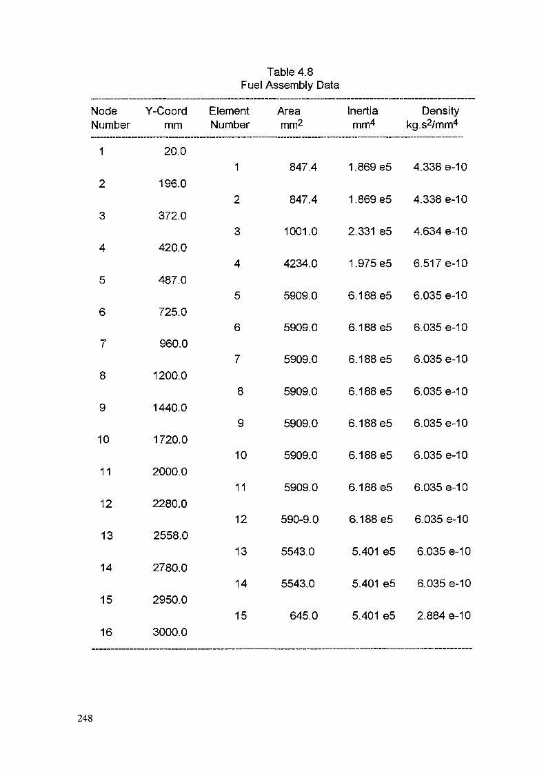
Table 4.8Fuel Assembly Data

Jode Y-Coord ElementJumber mm Number

1

2

3

4

5

6

7

8

9

10

11

12

13

14

15

16

20.0

196.0

372.0

420.0

487.0

725.0

960.0

1200.0

1440.0

1720.0

2000.0

2280.0

2558.0

2780.0

2950.0

3000.0

1

2

3

4

5

6

7

8

9

10

11

12

13

14

15

Areamm2

847.4

847.4

1001.0

4234.0

5909.0

5909.0

5909.0

5909.0

5909.0

5909.0

5909.0

590-9.0

5543.0

5543.0

645.0

Inertiamm4

1.86905

1.86905

2.331 e5

1 .975 e5

6.188e5

6.188e5

6.188e5

6.188e5

6.188e5

6.188e5

6.188e5

6.188e5

5.401 e5

5.401 e5

5.401 e5

Densitykg.s2/mm4

4.338e-10

4.338 e-10

4.6346-10

6.51 7 e-10

6.035e-10

6.035e-10

6.035e-10

6.0356-10

6.035e-10

6.0356-10

6.0356-10

6.0356-10

6.035e-10

6.0356-10

2.884 e-10

248

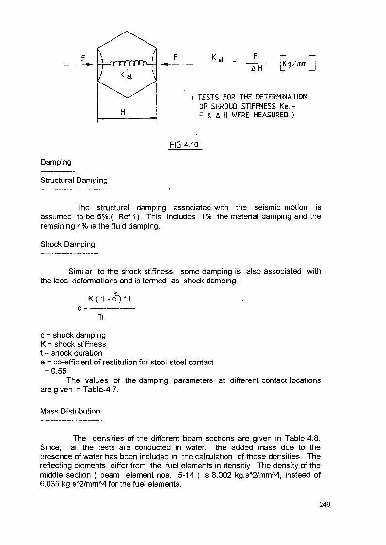
H

K el K g/mm

( TESTS FOR THE DETERMINATIONOF SHROUD STIFFNESS Kel-F & A H WERE MEASURED }

FIG 4.10

Damping

Structural Damping

The structural damping associated with the seismic motion isassumed to be 5%.( Ref.1). This includes 1% the material damping and theremaining 4% is the fluid damping.

Shock Damping

Similar to the shock stiffness, some damping is also associated withthe local deformations and is termed as shock damping.

K ( 1 - e) * t

c = shock dampingK = shock stiffnesst = shock duratione = co-efficient of restitution for steel-steel contact= 0.55

The values of the damping parameters at different contact locationsare given in Table-4.7.

Mass Distribution

The densities of the different beam sections are given in Table-4.8.Since, all the tests are conducted in water, the added mass due to thepresence of water has been included in the calculation of these densities. Thereflecting elements differ from the fuel elements in densitiy. The density of themiddle section ( beam element nos. 5-14 ) is 8.002 kg.sA2/mmA4, instead of6.035 kg.sA2/mmA4 for the fuel elements.

249

Experimental Measurements

Following experimental measurements were provided.

Test No.1 - AO top acceeleration Time History No. 4Test No.2 - AO top displacement Time History No. 8Test No.3 - AO top displacement Time History No. 12Test No.4 - AO top acceeleration Time History No. 62

B1 top acceeleration Time History No. 63B3 top acceeleration Time History No. 64B7 top acceeleration Time History No. 65B9 top acceeleration Time History No. 66

B11 top acceeleration Time History No. 67AO top displacement Time History No. 68A1 top displacement Time History No. 69A4 top displacement Time History No. 70B1 top displacement Time History No. 71B7 top displacement Time History No. 72

The numerical values were supplied in the form of diskettes.

4.3.3 Analysis

Analysis was carried out by using the general purpose finite elementcomputer code COSMOS. All the four configurations were analysed using themodal superposition approach.

4.3.3.1 Modal Superposition

This consists of performing a free vibration analysis of the beammodel, finding the natural frequencies and mode shapes and then performinga time history analysis with the desired number of modes.

Analysis Model

The hexagonal elements are modelled by using the beam elements ofthe finite element program. These beams are fixed at bottom. In the actualexperiment, the support configuration has clearances at the two contactspheres. This introduces a non-linearity, in the sense that the naturalfrequency of the elements depends on the excitation level. This observationwas made by Dr. Martelli. They had circumvented this problem by assuminga condition of fixity at the bottom and by adjusting the stiffness of the spike foreach level of excitation in such a way that the experimentally measured naturalfrequency of the element is simulated. The same approach is followed herealso. The Young's Modulus of the spike is adjusted to get the desirednatural frequency. For the 0 db level of excitation employed in the tests, the

250

first natural frequency of the fuel elements was 3.30 Hz and that of the reflectingelements was 3.0 Hz.

Free vibration analysis was performed and the first three modes wereextracted. The first three natural frequencies of the fuel element were 3.3Hz,22.1 Hz and 64.3Hz. Those for the reflecting element were 3.1 Hz, 19.9Hz and57.1 Hz. The clearances at the pad locations were modelled by using the 'gap1

elements in the time history analysis.

The structural damping is modelled as Rayleigh damping. For the 5%damping employed in the analysis, the values of the two co-efficients alpha andbeta are 0.095/sec and 0.002493 sec resp.

The gap elements used to model the clearances at the pad locationsincorporated the shock stiffness. But due to the limitations of the programcapabilities, the shock damping could not be modelled in this analysis. Non-linear analysis using direct integration method can account for this dampingbut takes enormous amount of computer time. The effect of neglecting this isdiscussed later.

A typical model for the 7 element configuration is shown in Fig 4.11.The model for other configurations is similar with the number of hexagonalrings appropriately changed. Although the figure shows the full model,analysis itself was performed for only half the model, utilising the condition ofsymmetry.

Time step of 1 ms was used in the analysis. The effect of reduced timestep was also studied.

4.3.4 Results & Discussion

Displacement vs time history plot of location Ao respectively fromanalysis, experiment and both superimposed (for comparison) are shown infigures 4.12 to 4.14, for the case of 19 element cluster (mixed). It can be seenthat the comparison is very good.

The results of the calculations are presented in Tables 4.9 & 4.10. Thetable gives the experimental and the theoretical values of the relativedisplacement ( maximum and RMS) and the total acceleration ( maximum andRMS ), at different locations for the different configurations studied.

The maximum and the RMS values ( measured and calculated) ofthe response can be compared with the maximum and RMS values of theexcitation and the magnification factor can be found. These factors for thedifferent configurations are given in Table 4.11.

251

-DIRECTION OF EXCITATION

PLANE OF SYMMETRY

PLAN VIEW <

N

77/+T7

77ÏÏ7T

\

///T//

777 *77

777777

TOP LOAD PAD

MIDDLE LOAD PAD

777^*77 BOTTOM GRID PLATE

77? *?7

7-ELEMENT CLUSTERMODEL FOR MODAL ANALYSIS

FIG/4,1V-'-

252

B-iResponse of 19 element cluster (mixed)

5.5 6.5 , 7.5 8.5Time in sees.

Figure 4.12

9.5

locot'on : AO

10.5 11.5

Response of 19 element cluster (mixed) location : AO

4-

_a.V) 0_

5 ~^

-4-

-6-Experiment

~T———1———1———T——I———I-

10.54.5 5.5 6.5 7.5 8.5Time in secs.

Figure 4.13

9.5 11.5

253

-6-

Response of 19 element cluster (mixed)

1. Experiment2. BARC/lndia

4.5 5.5 7.5 . 8.5Time in sees.

Figure 4.14

9.5 10.5 11.5

Table 4.9

Clusters with all fuel elements

Comparison of responses

acceleration- cm/s/s

expt. theory

displacement- cm

expt. theory

max. rms max rms max. rms max. rms

Single 1602 354 1084 373assembly

2.6 0.86

7-elementcluster

1246 372 2.44 0.74 2.9 0.86

19-elementclusterall fuel

1286 405 2.57 0.78 3.1 0.94

254

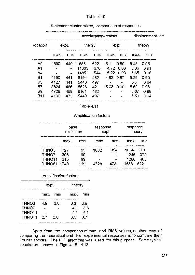
Table 4.10

19-element cluster mixed, comparison of responses

location expt.

acceleration- cm/s/s

theory expt.

displacement- cm

theory

max. rms max rms max. rms max. rms

AOA1A4B1B3B7B9B11

4590--

41904127382447284130

440--

441441466459473

11558116031485281945440562681615440

622676544482497421482497

5.14.725.224.82

-5.03

--

0.890.830.930.87

-0.90

--

5.455.365.655.295.55.595.675.50

0.950.910.960.900.940.980.980.94

Table 4.11

Amplification factors

base responseexcitation expt.

max. rms max. rms

THN03 327 99 1602 354THNO7 306 99THNO11 315 99THNO61 1748 169 4728 473

Amplification factors

expt. theory

max. rms max. rms

THN03 4.9 3.6 3.3 3.8THNO7 - - 4.1 3.8THNO11 - - 4.1 4.1THN061 2.7 2.8 6.6 3.7

responsetheory

max. rms

1084 3731246 3721286 405

11558 622

Apart from the comparison of max. and RMS values, another way ofcomparing the theoretical and the experimental responses is to compare theirFourier spectra. The FFT algorithm was used for this purpose. Some typicalspectra are shown in Figs. 4.15-4.18.

255

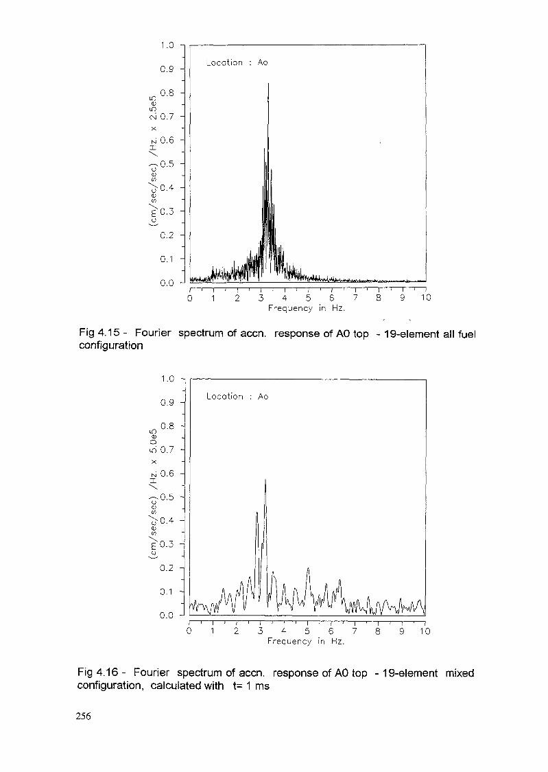
in

1.0 -i

0.9 -

0.7 -

N 0.6 -

— 0.5 -oO)en

>0.4 -CDin

0.2 -

0.1 -

0.0 J

l3 4 5 6 7

Frequency in Hz.

' — i10

Fig 4.15 - Fourier spectrum of accn. response of AO top - 19-element all fuelconfiguration

1.0 -,

0.9 -

n 0.8 -moLO 0.7 -X

N 0.6 -

o<uCO\o0)

-0.5 -

0.4 -

0.3 -

0.2 -

0.1 -

0.0 -

Location : Ao

2 3 4 5 6 7Frequency in Hz.

10

Fig 4.16 - Fourier spectrum of accn. response of AO top - 19-element mixedconfiguration, calculated with t= 1 ms

256

160

15 20Frequency in Hz

25 30

Fig 4.17 - Fourier spectrum of accn. response of AO top - 19-element mixedconfiguration, experimentally measured

o.o20

Frequency in Hz

Fig 4.18- Fourier spectrum of accn. response of AO top -19-element mixedconfiguration, calculated with t =0.1 ms

257

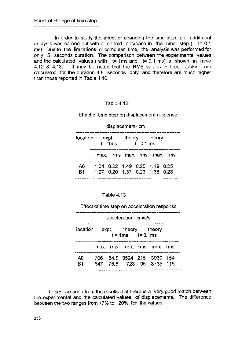
Effect of change of time step

In order to study the effect of changing the time step, an additionalanalysis was carried out with a ten-fold decrease in the time step ( t= 0.1ms). Due to the limitations of computer time, the analysis was performed foronly 5 seconds duration. The comparison between the experimental valuesand the calculated values ( with t= 1ms and t= 0.1 ms) is shown in Table4.12 & 4.13. It may be noted that the RMS values in these tables arecalculated for the duration 4-8 seconds only and therefore are much higherthan those reported in Table 4.10.

Table 4.12

Effect of time step on displacement response

displacement- cm

location expt. theory theoryt = 1ms t= 0.1 ms

max. rms max. rms max. rms

AO 1.04 0.22 1.49 0.25 1.49 0.25B1 1.27 0.20 1.37 0.23 1.38 0.23

Table 4.13

Effect of time step on acceleration response

acceleration- cm/s/s

location expt. theory theoryt = 1ms t= 0.1ms

max. rms max. rms max. rms

AO 706 84.5 3524 215 3939 154B1 647 75.8 723 95 3735 115

It can be seen from the results that there is a very good match betweenthe experimental and the calculated values of displacements. The differencebetween the two ranges from +7% to +20% for the values.

258

For acceleration, however, the discrepancy is much larger. Thecorresponding differences range from -30% to +150% for the maximum values,and from -10% to +41 % for the RMS values.

The major shortcoming in the calculations was that shock dampingwas not accounted for. Obviously, the displacements are not affected by theshock damping. Therefore, the reactivity changes, which are function ofdisplacement response, can be well predicted even without shock damping.However, for accurate prediction of accelerations and in turn, the contactforces between the elements at the contact pads; shock damping isimportant. The importance of the shock parameters viz. shock stiffness andshock damping; in determining the acceleration and force response wasbrought out in Stage-l results. As stated earlier, the reason for not includingthe shock damping was the enormous amount of computer time required when itis included.

Effect of time step

From the comparison of the responses given in Tables 4.12 & 4.13, itcan be seen that as far as displacement response is concerned, there ispractically no change in response due to ten-fold decrease in the time step.However, the acceleration response does change. Even here, the change inRMS values is not as much as the change in the maximum values.

4.4 MONJU - CORE TESTS

4.4.1 Problem Definition

Defined by:

experiments conducted at: PNC, JAP AN.

This problem consists of the following cases,

i) Seismic test on 29 assemblies in a single row

ii) Seismic test on 37 fuel assemblies in matrix layout

The testing configurations for the two cases are shown in figure 4.19.The tests were carried out both in air and in water.

This report presents the results of the calculations performed for thetests in water.

259

MONJU CORE AND TEST CONFIGURATIONS

SINGLE ROW MODEL(29 CORE ELEMENTS)

CLUSTER MODEL(37 FUEL ASSEMBLIES)

4.19

4.4.2 Input datas

4.4.2.1 Geometrical Details

The mock-ups of Monju core simulate the dimensions and mass andstiffness distributions of the actual assemblies.

The geometry and mass distribution data for Fuel Assembly (F/A),Radial Blanket Assembly (R/B) and Neutron Shield Assembly (N/S) are listed inTables I through III respectively.

For the tests conducted in water, the added mass due to the presence ofwater has been included in the calculation by adjusting the densities.

The fuel and blanket and shielding assemblies are separated fromeach other through small clearances ( gaps ) at the pad locations. The nominalvalues of the gaps are;

0.7 mm at top load pads (TLP)1.0 mm at middle load pad (MLP)

4.4.2.2 Stiffness Properties

Beam Properties

The hexagonal elements are modelled as beams. The stiffnessproperties of the beams; cross-sectional area, moment of inertia are as given inTables 4.1 to 4.3.

260

Shock Stiffness

When the elements strike each other at the pad locations during theseismic motion, there is a local deformation of the faces of the hexagons. Thestiffness associated with this is termed as shock stiffness. This is evaluated byconducting tests on the elements, in which, the force and the deformation aremeasured. The stiffness values at the two pad locations are given below.

T.LP. M.L.P.

F/A 7.0 E04 kg/mm 1.2 E03 kg/mm

R/B 7.0 E04 kg/mm 1.2 E03 kg/mm

N/S 7.0 E04 kg/mm 1.2 E03 kg/mm

DAMPING

Structural Damping

The structural damping associated with the seismic motion is assumedto be 3% for fuel and blanket assemblies and 2 % for the shielding assembliesfor the first mode and 15% for all higher modes .

Shock Damping

Similar to the shock stiffness, some damping is also associated withthe local deformations and is termed as shock damping. The value of the shockdamping is 11 %.

Supporting Condition

The assemblies are assumed to be pinned at the top and the bottomplates of the core support structure (diagrid).

Instrumentation

Accleration, relative displacement, impact force and strain were measured attypical locations.

Figure no. 4.20 shows the instrumentaion locations for the row model testwhile figure 4.21 shows these locations for the cluster model tests.

261

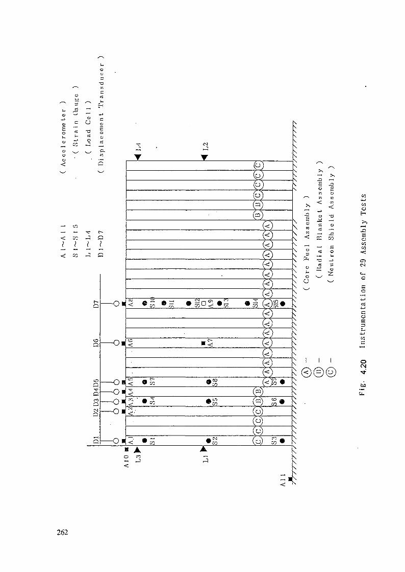
Oü

0

oci

0o

L L<; M

? ?

(o)

(<0

coVI

l(*)

»S

< «• A A

3

TCJ

"P

"®

OT '

ny.

^ CO

ti o— ~

WO

O

Cü O

O

C3

O

5

Oc\

262

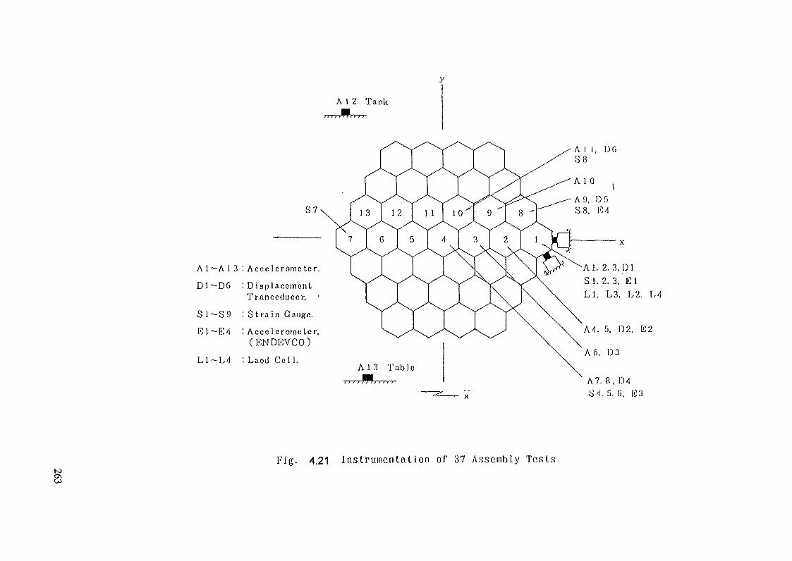
A l 2 TankTT f yi^^/T^n 7~

A1~-A 1 3 '• A c c e l e r o m c t e r .

D1~D6 : D i s p l a c e m e n tTranccducer .

S 1~S9 : S t r a i n Gauge.

El~-E ' l ' • A c c c l o r o m e ter.(ENDEVCO)

Ll-L'l : Laod C e l l .

A 9, 05S 8. E'i

\

— x

Al. 2. 3. DlSi. 2. 3. ElLI. L3. L2. L 4

A'). 5. D2, E2

A 6, D3

A7. 8, D4SI. 5. 6. E3

Fig. 4.21 Instrumentation of 37 Assembly TestsK)

Seismic Input

The original acceleration time history which was used for giving input toshaking table was supplied by PNC. For the 400 gal test level theaccelerations were scaled by a factor 400/897.1.

4.4.3.0 Analysis

Analysis was carried out by using the general purpose finite elementcomputer code COSMOS. All the test configurations were analysed using themodal superposition approach.

4.4.3.1 Modal Superposition

This consists of performing a free vibration analysis of the beam model,finding the natural frequencies and mode shapes and then performing a timehistory analysis with the desired number of modes.

Analysis Model

The hexagonal elements are modelled by using the beam elements ofthe finite element program. These beams are pinned at two locations.

Free vibration analysis was performed and the first three modes wereextracted. The clearances at the pad locations were modelled by using the'gap' elements in the time history analysis.

The structural damping was modelled as modal damping.

The gap elements used to model the clearances at the pad locationsincorporated the shock stiffness. But due to the limitations of the programcapabilities, the shock damping could not be modelled in this analysis.

The row model consists of beam elements arranged in a row with thegaps and the associated springs on both sides of each element.

A typical model for the 7 element cluster configuration is shown in Fig4.11. The model for 37 element configurations is similar with the number ofhexagonal rings appropriately changed. Although the figure shows the fullmodel, analysis itself was performed for only half the model, utilising thecondition ofsymmetry.

Time step of 0.025 ms was used in the analysis.

264

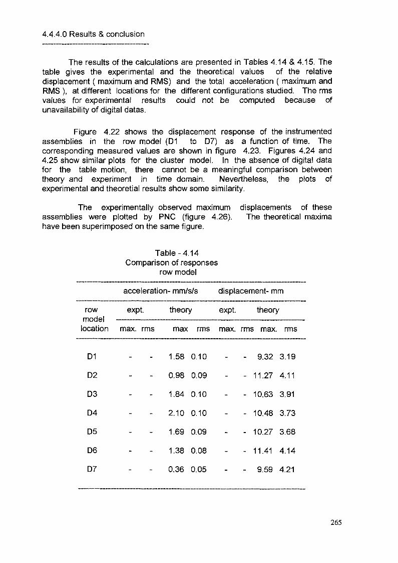
4.4.4.0 Results & conclusion

The results of the calculations are presented in Tables 4.14 & 4.15. Thetable gives the experimental and the theoretical values of the relativedisplacement ( maximum and RMS) and the total acceleration ( maximum andRMS ), at different locations for the different configurations studied. The rmsvalues for experimental results could not be computed because ofunavailability of digital datas.

Figure 4.22 shows the displacement response of the instrumentedassemblies in the row model (D1 to D7) as a function of time. Thecorresponding measured values are shown in figure 4.23. Figures 4.24 and4.25 show similar plots for the cluster model. In the absence of digital datafor the table motion, there cannot be a meaningful comparison betweentheory and experiment in time domain. Nevertheless, the plots ofexperimental and theoretial results show some similarity.

The experimentally observed maximumassemblies were plotted by PNC (figure 4.26).have been superimposed on the same figure.

displacements of theseThe theoretical maxima

Table-4.14Comparison of responses

row model

rowmodel —————location max. rms

D1

D2

D3

D4

D5

D6

D7

acceleration- mm/s/s

expt.

displacement- mm

theory expt. theory

max rms max. rms max. rms

1.58

0.98

1

2

1

1

0

.84

.10

.69

.38

.36

0.

0

0,

0

0.

0,

.10

.09

.10

.10

.09

.08

0.05

- 9

- 11

- 10

- 10

- 10

- 11

.32

.27

.63

.48

.27

.41

- 9.59

3

4

3

3

3

4

4

.19

.11

.91

.73

.68

.14

.21

265

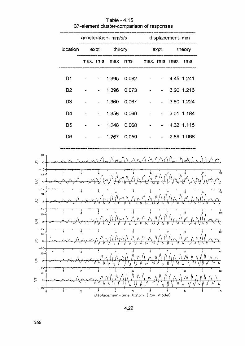
Table-4.1537-element cluster-comparison of responses

acceleration- mm/s/s

location expt. theory

D1

D2

D3

D4

D5

D6

max. rms max rms

- 1.395 0.082

- 1.396 0.073

- 1.360 0.067

- 1.356 0.060

- 1.248 0.068

- 1.267 0.059

displacement- mm

expt. theory

max. rms max. rms

4.45 1.241

3.96 1.216

3.60 1.224

3.01 1.184

4.32 1.115

2.89 1.068

10-

Q An-10-

10-?

CMa

10

4,fA A.ö V K

-10-

10 n°

A . .i ' i '

AftA.MA' U u W .u u '

10

\j£\U ^

-10-

10n°

•3-O

10

-10-

10-

A,. ..A. A \tt-10-

v v v w v v~1———r

410-

,sA/V^VN-10-

»On°f\ f\ A A

10

v - y v n/wvr3 4 5 6 7

Displacement-time history (Row model)

4.22

10

266

1)1 1)1, 1)7

'A U A A _L__L

i . l^-^_—, /vVvvV^-v^~A'V*^"V\^^

^-J \0 I? ( m i x )

to

423 Di sp l acemen t Tune H i s t o r y (400gal , In W a t e r )

Q

10-1

0 A / A f J \ f A - " A

-10-

10n°

Q

10

-On°~

10

-10-

10 n°

J f i A A ^ A A A A^Vt

10

-10-———r n——i——i——'——r1 2 3

~l———i———I———i———T5 6 7

g 0-

-IQ-

10

.0-?

toQ 0-

I i I8 9

~110

-10-3 4 5 6 7

Displacement—time history (cluster model)

I10

4.24

S1U ßa.N,o'

•s

< $iii\ei^^^^

i^f^w^fi^^„—..V,„,N~J,Y.V -,'vVY^sVvr,™

A/We Ace

Fig 425 Disp lacement Time H i s t o r y ( « i O O g a l , In Wate r )

268

EXAMPLE OF TEST DATA (SINGLE ROW TEST)

10

i n vva 1erO 20 0 gal• «I 0 0 ga 1

10 15Component Number

DISTRIBUTION OF MAX. DISPLACEMENTTO S1 EARTHQUAKE EXCITATION4.26

Apart from the comparison of max. and RMS values, another way ofpresenting the theoretical and the experimental response is to compute theirFourier spectra. Figs.4.27 & 4.28 show the spectum for displacement response,figure 4.27 shows a clear peak at 3.3 Hz, the first natural frequency.

It can be seen from the results that there is a resonably good matchbetween the experimental and the calculated values of displacements.

The major shortcoming in the calculations was that shock damping wasnot accounted for. This suggests that the displacements are not affectedby the shock damping and the reactivity changes, which are function ofdisplacement response, can be well predicted even without shock damping.However, for accurate prediction of accelerations and in turn, the contactforces between the elements at the contact pads; shock damping is probablyimportant.

The computer code being used for the seismic analysis of LMFBR coresis capable of predicting the displacement response of the assemblies with areasonable accuracy. The same cannot bew said of the acceleration or theimpact force response, but cause of this may lie in the modelling of the shockparameters which, at present, is based on the static tests.

5.0 CONCLUSIONS

The computer code COSMOS/M used for seismic analysis has a fewshortcomings as follows:

269

1200

1000

800

600

400

200

0 1

FFT of Displacement Response D1 (Row model)Figure 4.27

1000

900

800

700'

600

500

400'

300'

200'

100-

0-0 2 4 6 8 10 12 14 16 18 20

Frequency in Hz

FFT of displacement Response D1 (cluster model)Figure 4.28

270

- inability to model shock damping in modal superposition method. This may notbe a serious shortcoming because the calculated results without shock dampinghave shown good match for displacement response which is the primaryresponse of concern.

-Limitation on the number of gaps (150) , which makes it unsuitable for theanalysis of a large cluster such as Rapsodie mock-up. Although this will be ahandicap when core of the actual reactor is analysed, this too may not beserious because a large core can be analysed using a row model. This reducesthe problem size considerably and the solution is very close to the experimentalvalues.

The computer code COSMOS/M has been validated for seismicanalysis of LMFBR cores.

6.0 RECOMMENDATIONS FOR FURTHER STUDIES

As future extension of the program the following suggestios aremade.

- Its forward integration into a reactivity calculation program.- Its backward integration into a code for seismic analysis of reactor block.

Since the seismic motion of diagrid is an input to the core analysis it needs to beput on a firm footing by validating the modelling aspects and the codes whichperform these calculations.

REFERENCES

1) Martelli.A., Gauvain.J & Bernard.A., "Non-linear Dynamic andSeis mic Analysis of Fast Reactor Cores — 1 — TheoreticalModel", SMiRT-6

2) Martelli.A., "Methods for the Seismic Verification of a FastReactor Core", SMiRT-8.

3) Brochard.D., " Seismic Behaviour of LMFBR Cores "., SMiRT-8

4) Di Giamberardino., et al,"Study of the Structural Behaviourof PEC reactor fuel Element Sub-Assembly Support Charged byDesign Earthquake", SMiRT-8

5) Bonacina.G., et al., "Response ot Impacts of Fast ReactorCore Bêlements During Seismic Excitation", SMiRT-8

6) Bonacina.G., Castoldi.A., &Zola.M., "Dynamic and SeismicResponse in Air and Water of Prototypic Models of PEC FastReactor Core Elements", SMiRT -

271

7) Cecchini.F et al., "Feed-Backs on PEC Fast Reactor CoreDesign due to Seismic Conditions and Main NumericalResults", SMiRT-

8} Castoldi.A., "Experimental demonstration of the PEC FastReactor Scramability in the Case of Earthquake", SMiRT-

9) Neri.P., "Experimental Tests for Structural and FunctionalVerifications of PEC Fast Reactor Core Elements with SeismicLoadings", SMiRT -

10) Martelli.A., et al., 'Vessel-Core Seismic Interaction for aFast Reactor", smlrt-7

11 ) Gantenbein.F., et al., "Seismic Behaviour of a Fast Reactorcore. Application on SUPER PHENIX I", SMiRT-7

12) Bonacina.G., etal., "Dynamic and seismic Behaviour of PECreactor Core elements; Comparison Between computed andexperimental Results", SMiRT-7

13) Sasaki.Y., et al., "Experimental Studies on SeismicVibration Phenomena of FBR core Components", SMiRT-7

272

ANNEX IADVANCEMENT IN THE SEISMIC ANALYSIS OF COMPLEX

REACTOR BUILDING STRUCTURES

G.R.REDDY, K.K.VAZE, H.S.KUSHWAHA K.V.Subramanian, J.V.TandaleReactor Engineering Division Tata Consulting Engineers .Bhabha Atomic Research Centre 414-Veer Savarkar MargBombay-400085, India Prabha Devi, Bombay-400025

ABSTRACTSeismic analysis oî complex Nuclear Reactor Building is carried out

using lumped mass beam model. Beam model is used because of its simplicityand economy. Beam properties like area, shear area , moment of inertia arecalculated using classical equations available in the literature. Theseproperties are used for stiffness calculation. Masses are lumped at differentnodal points. In this paper, difficulties of evaluating the properties usingclassical equations are explained. A simple,accurate and a new procedurewhich overcomes the difficulties is explained. Also validity of the procedure isbrought out.

2.0 INTRODUCTION

The Reactor Building (RB) as shown in fig.1 consists of Internal Structure(IS) and Calandria Vault (CV) contained in a coaxial inner and outercontainment walls (ICW and OCW) cast monolithically with a circular raft at EL85000. The OCW consists of cylindrical RCC wall of die 54.72 msupporting RCC torispherical dome. The ICW consists of prestressedcylindrical wall of inner dia 49.5 and supports a prestressed concretetorispherical dome with a steel liner.

The CV as shown in fig.2 is a tall, hollow, rectangular box made of heavyconcrete. In the north and south walls of vault, there is an octoganal openingto house the calandria endshield assembly. Calandria endshield assembly issupported by diaphragm plates. The diaphragm is a flexible member along N-Sdirection to accommodate the axial thermal expansion of calandria assembly.The calandria is fixed to the vault through 4 keys. The purpose of the keys is tokeep the calandria , reactivity and shutdown mechanisms in position duringearthquake. Calandria consists of main shell, subshell and annular plate .

The annular plate connets the main shell and subshell. The other end ofthe subshell is connected to the endshield assembly. Calandria housescalandria tubes, pressure tubes and fuel bundles. It is filled with heavy waterand submerged in light water in the vault. Endshiel consists of two tube sheetsjoined by 392 lattice tubes. Each lattice tube houses endfitting which isconnected to pressure tube. The space between lattice tubes and tube sheets isfilled with carbon steel balls and water.

The IS is a complex three dimensional structure consisting of following

a. Structural frame work consisting of columns and beams,b. Reinforced concrete beams, columns and thick shear walls,c. Prestressed concrete pressure walls.

273

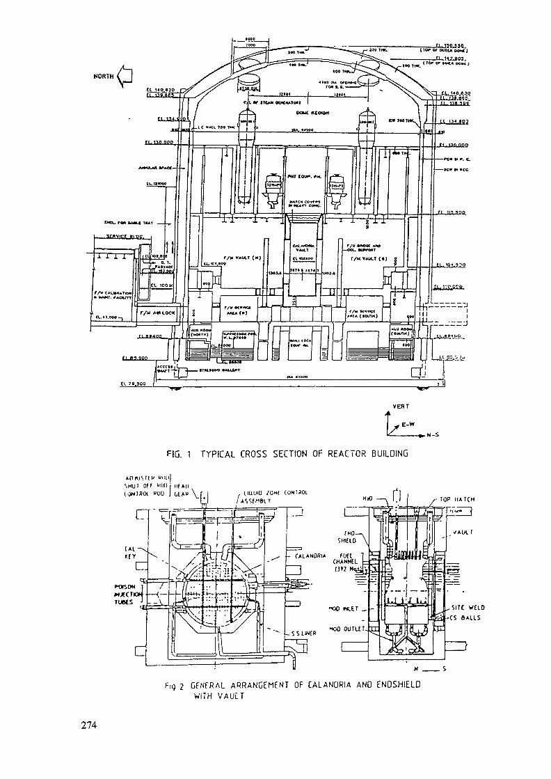
NORTH

) I ' I«LUMWHJACCCS* I L__.1»WT *^-f 3——— lIMfM*« «MUHT

.300 /

VERT

-».N-S

FIG. 1 TYPICAL CROSS SECTION OF REACTOR BUILDING

funSHUT Off "Oll l ilf All(OMJRCX. »ou j UAH Vf, UUUIÜ /UNI CON IDOL

- TOP M A T C H

- CALANORIA FU(lCHANNEL!3»2

- S S L W E R

Fig 2 GENERAL ARRANGEMENT OF CALANÜRIA AND ENDSHIELOWITH V A U Î T

214

The IS is symmetric about EW axis but unsymmetric about NS axis as infig 3-5. From EL 85000 to EL 100000 is a closed massive section as shown inflg.3. From EL 100000 TO EL 115000 it is an open section as shown in fig.4.At EL 104500 there is an offset in the section along north south direction andfrom there pressure walls are going upto EL 115000. These pressure walls aresupported by a slab at EL 104500. This slab is supported by north or south wallat one end and two concrete columns at the other end. Above 115500 there aretwo boxes (fig.5) housing the steam generators (SG). The east west walls ofeach SG is supported on walls below it. The north and south wall though restingon slab at EL 115500, spans as deep beam between east and west walls. TheIS and ICW are connected by an annular steel plate at EL 130000 as the IS isflexible above 115500. This link permits transfer of lateral force but allows thetwo structures to rotate independent of each other.

Calculating beam equivalent stiffness of containments is not a difficultproblem. It was earlier [1] shown that beam equivalent stiffness evaluatedusing classical formulae will represent a simle structure properly andproduce accurate response for seismic loads. However, evaluating equivalentbeam properties of complex IS using classical formulae may not representthe structure properly and hence a method based on strain energyequivalence is applied and beam equivalent properties were calculated .The details of the procedure are explained in subsequent sections.

Though CV along with calandria endshield assembly may behave like shearcantilever beam [2], and classical formulas may be sufficient for calculatingbeam properties, here it is tried to apply method of strain energy equivalenceto calculate beam equivalent properties and compare with classical formulas.

K 8

? 5 I t j 25 l 7C

FIG. 3. PLAN AT ELEVATION es o m OF is (INTERNAL STUCTUREJ

275

»iN -

7771

»12

7TT£

ie.7»

IT

I 75 L II td »«

f! «

o-,i 01:T

Het

10, 3i iiri

W

1070 ii

FIG. 4. PLAN AT ELEVATION 104.5 m OF IS

I I

»o»

W

i

-s 8

«72

l»2l

7400

l 2072

FIG. 5. HALF PLAN AT ELEVATION 115.5-130.0» OF IS

276

Jktf MODELLING TECHNIQUES:

3.1 CONVENTIONAL 2D BEAM MODEL:

This is the simplest model (Fig.6) one can make for analysisngstructures. Here it is assumed that the structure behaves like cantilever beamand classical beam assumptions like plane sections remain plane before andafter deformation, rigid connections between two sections etc. Floors areassumed rigid. Mass of the structure is lumped at series of points [1] at centre ofthe building. The beam section properties are calculated using classicalformulae[3] and are given in table. 1. Effects of slabs flexibility, offset at EL114500, partial support of SG box north and south walls is neglected.TheOCW is represented by 23 elements, ICW is represented by 21 elements.The IS is represented by represented by 2 elements and the transverse,vertical, rotational and torsional springs are applied at the raft level to cater tothe effect of soil-structure interaction (ASCE 4-86). All the substructures arerepresented at the centre of the building. The connection between the IS andICW at EL 130000 is modelled using springs representing the stiffness ofthe connecting link at the respective nodes.

sac w i

Kx * TRANSLAT1ONALSPRING

K« » ROTATIONALSPRING

CWTERNALS1o

® r " OICAU1NORIA!i i3 .îaoz«

- V "5 JO5 3<

HALf SECTION OF REACTCP BULDIMGK . - «

MATHEMATICAL MODEL FORSEISMIC ANALYSIS

MODEL OF REACTOR BUILDING FOR ROCKY SITE

FIG. 6. 2D BEAM MODEL OF REACTOR BUILDING

277

Table. 1. Comparison of sectional properties for IS

SECTION SHEAR MI@EW SHEAR MI@NS AREAAREA m AREA m m

NS m

J CENTRE OFm RIGIDITY

EW(m) NS(m)

EL 85- 93EL 93-1 00EL 93-1 04EL104-109

EL109-115EL115-130

FORMFEM

FORMFEM

FORMFEM

FORMFEM

FORMFEM

FORMFEM

27317115610312464

1211091291144222

2106527630116403616551532475164330453044451551322

265227114449734291029105638

460311831040354156209132106403378105403378571937125137

43039223417619294

151110153709057

101039743122

17030120

1255392

9911108

1097512612660

0.00.00.00.00.00.0

-0.85-2.25-2.200.140.640.48

ZQ. 3D STICK MODEL BASED ON STRAIN ENERGY EQUIVALENCE

In this method of modelling, beam stiffness is calculated using strainenergy equivalence [5,6] of the beam model and 3D finite element model(FEM). In this .unlike above method , the effect of flexibility of floors, offset atEL 104500, partial support of SG box north and south wall is accounted andprocedure is explained below.

A 3D FEM model is made as shown in fig.7. Though columns, beams andfloors external to the shear wall structure are modelled, they are not shown

MOOE1.

FIG. 1. MATHEMATICAL MODELS OF REACTOR IS

278

in this figure for clarity. Thin plate and shell element are used for modellingslabs walls. Shear beam elements are used for modelling columns and beams offloors.

3:2.1 Centre of rigidity and Torsional inertia

Centre of rigidity of a section is obtained by evaluating the torsional centre,as in the linear domain both are same point on the crosssection. For differentsections of the internal structure , torsional moments are applied, and thepoint on each section where horizontal displacement is zero is determined. Thisis the torsional centre. For determination of torsional inertia for the elementsof the beam representing the IS, torsional loads are applied on the full FEM

3.0 MODELLING TECHNIQUES:

3.1 CONVENTIONAL 2D BEAM MODEL:

This is the simplest model (Fig.6) one can make for analysisngstructures. Here it is assumed that the structure behaves like cantilever beamand classical beam assumptions like plane sections remain plane before andafter deformation, rigid connections between two sections etc. Floors areassumed rigid. Mass of the structure is lumped at series of points [1] at centre ofthe building. The beam section properties are calculated using classicalformulae[3] and are given in table. 1. Effects of slabs flexibility, offset at EL114500, partial support of SG box north and south walls is neglected.TheOCW is represented by 23 elements, ICW is represented by 21 elements.The IS is represented by represented by 2 elements and the transverse,vertical- rotational and torsional springs are applied at the raft level to cater tothe effect of soil-structure interaction (ASCE 4-86). All the substructures arerepresented at the centre of the building. The connection between the IS andICW at EL 130000 is modelled using springs representing the stiffness ofthe connecting link at the respective nodes.

3,2 3D STICK MODEL BASED ON STRAIN ENERGY EQUIVALENCE

In this method of modelling, beam stiffness is calculated using strainenergy equivalence [5,6] of the beam model and 3D finite element model(FEM). In this ,unlike above method , the effect of flexibility of floors, offset atEL 104500, partial support of SG box north and south wall is accounted andprocedure is explained below.

A 3D FEM model is made as shown in fig.7. Though columns, beams andfloors external to the shear wall structure are modelled, they are not shownin this figure for clarity. Thin plate and shell element are used for modellingslabs walls. Shear beam elements are used for modelling columns and beams offloors.

3.2.1 Centre of rigidity and Torsional inertia

Centre of rigidity of a section is obtained by evaluating the torsional centre,as in the linear domain both are same point on the crosssection. For different

279

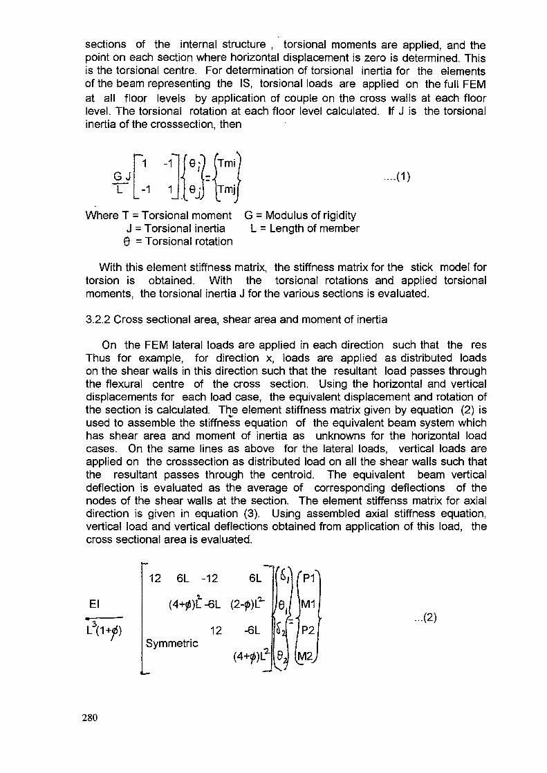
sections of the internal structure , torsional moments are applied, and thepoint on each section where horizontal displacement is zero is determined. Thisis the torsional centre. For determination of torsional inertia for the elementsof the beam representing the IS, torsional loads are applied on the full FEMat all floor levels by application of couple on the cross walls at each floorlevel. The torsional rotation at each floor level calculated. If J is the torsionalinertia of the crosssection, then

G J1 -1

-1 1....(1)

Where T = Torsional moment G = Modulus of rigidityJ = Torsional inertia L = Length of member0 = Torsional rotation

With this element stiffness matrix, the stiffness matrix for the stick model fortorsion is obtained. With the torsional rotations and applied torsionalmoments, the torsional inertia J for the various sections is evaluated.

3.2.2 Cross sectional area, shear area and moment of inertia

On the FEM lateral loads are applied in each direction such that the resThus for example, for direction x, loads are applied as distributed loadson the shear walls in this direction such that the resultant load passes throughthe flexural centre of the cross section. Using the horizontal and verticaldisplacements for each load case, the equivalent displacement and rotation ofthe section is calculated. The element stiffness matrix given by equation (2) isused to assemble the stiffness equation of the equivalent beam system whichhas shear area and moment of inertia as unknowns for the horizontal loadcases. On the same lines as above for the lateral loads, vertical loads areapplied on the crosssection as distributed load on all the shear walls such thatthe resultant passes through the centroid. The equivalent beam verticaldeflection is evaluated as the average of corresponding deflections of thenodes of the shear walls at the section. The element stiffenss matrix for axialdirection is given in equation (3). Usjng assembled axial stiffness equation,vertical load and vertical deflections obtained from application of this load, thecross sectional area is evaluated.

El

12 6L -12 6L

(4+0)L-6L (2-0)1^

12 -6LSymmetrie

•t]t*&2

B2

I* *\P1M1

P2

M2j

...(2)

280

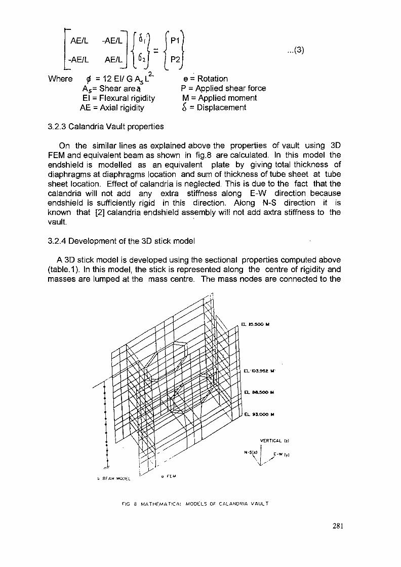
AE/L -AE/L

-AE/L AE/L

P1

Where 0 =12EI/GASLA5= Shear are %El = Flexural rigidity

AE = Axial rigidity

3.2.3 Calandria Vault properties

P2L J

...(3)

e = RotationP = Applied shear forceM = Applied moment& = Displacement

On the similar lines as explained above the properties of vault using 3DFEM and equivalent beam as shown in fig.8 are calculated. In this model theendshield is modelled as an equivalent plate by giving total thickness ofdiaphragms at diaphragms location and sum of thickness of tube sheet at tubesheet location. Effect of calandria is neglected. This is due to the fact that thecaiandria will not add any extra stiffness along E-W direction becauseendshield is sufficiently rigid in this direction. Along N-S direction it isknown that [2] calandria endshield assembly will not add axtra stiffness to thevault.

3.2.4 Development of the 3D stick model

A 3D stick model is developed using the sectional properties computed above(table.1). In this model, the stick is represented along the centre of rigidity andmasses are lumped at the mass centre. The mass nodes are connected to the

EL K.50O M

EX'»03.952 M'

EL »&SOO M

t, Bf AM MODEL

F!G 8 MATHEMATICAL MODELS OF CALANDRIA VAULT

281

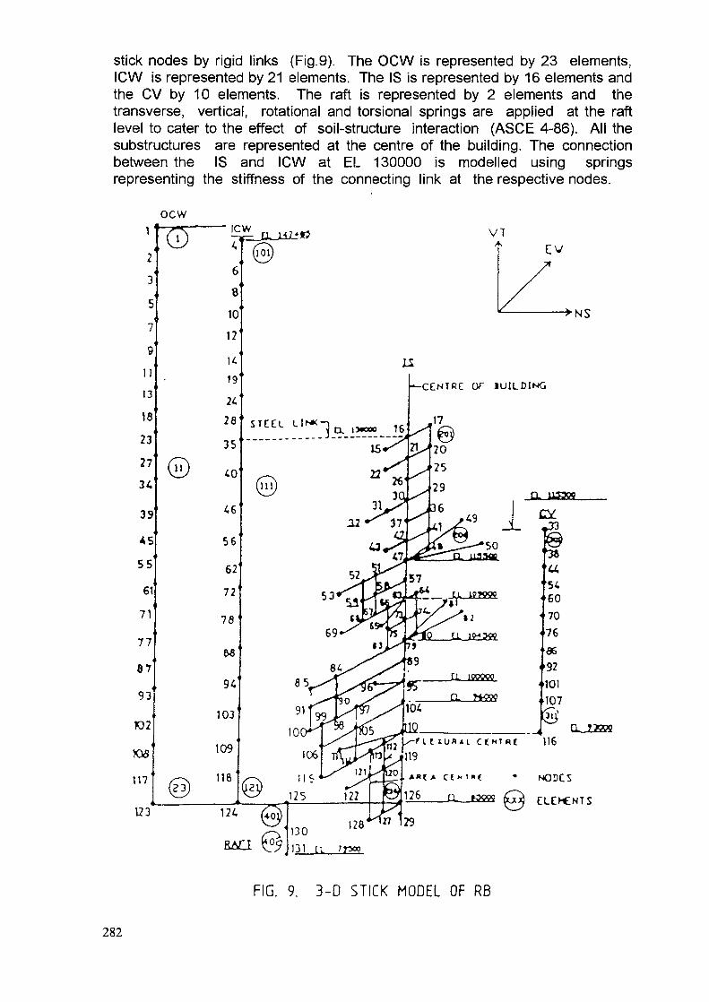
stick nodes by rigid links (Fig.9). The OCW is represented by 23 elements,ICW is represented by 21 elements. The IS is represented by 16 elements andthe CV by 10 elements. The raft is represented by 2 elements and thetransverse, vertical, rotational and torsional springs are applied at the raftlevel to cater to the effect of soil-structure interaction (ASCE 4-86). All thesubstructures are represented at the centre of the building. The connectionbetween the IS and ICW at EL 130000 is modelled using springsrepresenting the stiffness of the connecting link at the respective nodes.

OCW

>NS

*-CENTRC OT JUILDING

RATT

FIG. 9. 3-D STICK MODEL OF RB

282

4.0 STRAIN ENERGY EQUIVALENCETo establish the equivalence of the 3D stick model as representing the

IS , the total strain energy in the two models (FE an 3D stick of substructureIS) for an arbitrary loading system is compared.

The strain energy U is equal to the work done in distorting the system.

U = 1/2OK -5 -.(4)

But, P = K£or PT=6K; HenceU=&1/2 P '....(5)

Where ° = displacement vector, K = Global stiffness matrix,P = total load vector

An eccentric load applied on the structure, causes all the displacementcomponenets, depending upon the eccentricity between the flexural centre andthe centre of applied loads. The strain energy viz. internal work done as perequqtion (4) is equal to the external work done computed using equation (5).

An arbitrary system of loads is applied at all levels in all the threedirections(two horizontal and one vertical)and torque is also applied at alllevels about vertical axis and the corresponding strain energies in the 3Dstick model and FEM of the IS are compared. The comparison is reported intable.4.

5.0 ANALYSIS

Dynamic analysis using 2D beam model and 3D beam model wasperformed. Frequencies and participation factors were calculated and are givenin table.3

6.0 VALIDATION OF BEAM MODELS

6.1 Analysis by Varying the load set

To find the independency of the equivalent stiffness of IS evaluated usingenergy equivalence method with respect to the load set considered, sixtypical load sets as shown in fig. 10 have been considered and using energyequivalence beam properties were evaluated and are shown in table.5. Staticdeflection for a general loading (fig. 10, GEN-LC)and for the six sets ofproperties was calculated using 3D stick model and tabulated in table.6. It canbe seen that variation in displacement is negligible. Dynamic analysis wascarried out using six sets of properties. Frequencies and the participationfactors are shown in table.7-8 respectively. The variation in frequencies andparticipation factors is negligibly small. Though, results are shown for N-Sdirection, for all other directions ( E-W, Vert) results were compared and foundin good agreement [6].

283

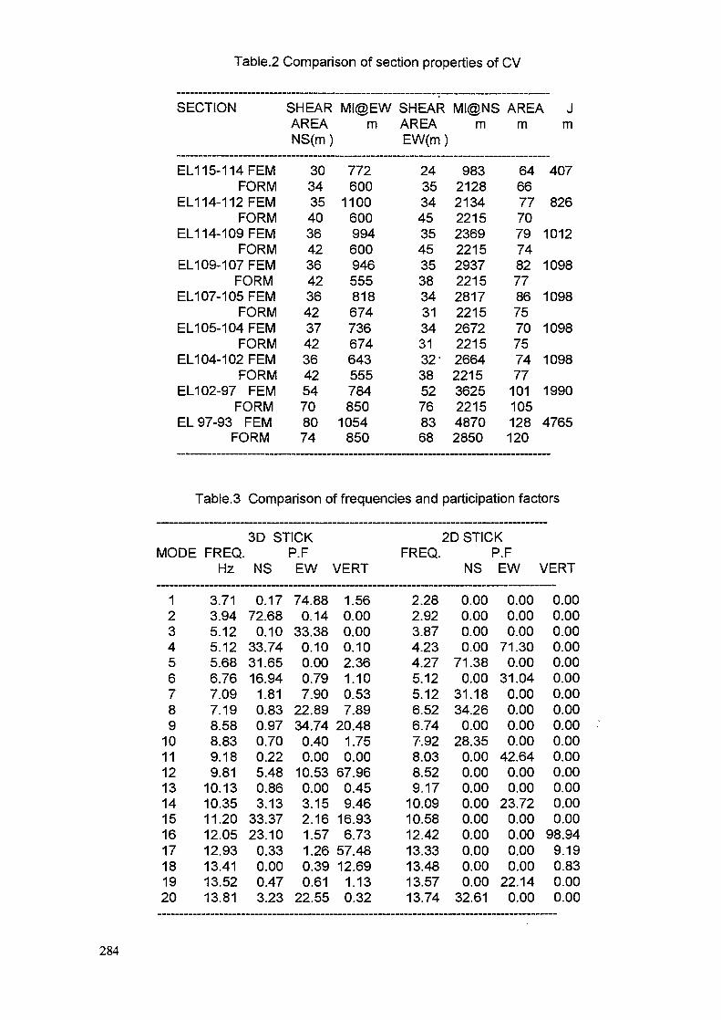
Table.2 Comparison of section properties of CV

SECTION SHEAR M!@EW SHEAR M1@NS AREA JAREA m AREA m m mNS(m ) EW(m )

EL11 5-114 FEM 30 772FORM 34 600

EL1 14-1 12 FEM 35 1100FORM 40 600

EL1 14-109 FEM 36 994FORM 42 600

EL109-107 FEM 36 946FORM 42 555

EL107-105 FEM 36 818FORM 42 674

EL105-104 FEM 37 736FORM 42 674

EL104-102 FEM 36 643FORM 42 555

EL1 02-97 FEM 54 784FORM 70 850

EL 97-93 FEM 80 1054FORM 74 850

24 983 64 40735 2128 6634 2134 77 82645 2215 7035 2369 79 101245 2215 7435 2937 82 109838 2215 7734 2817 86 109831 2215 7534 2672 70 109831 2215 7532' 2664 74 109838 2215 7752 3625 101 199076 2215 10583 4870 128 476568 2850 120

Table.3 Comparison of frequencies and participation factors

3D STICKMODE FREQ. P.F

Hz NS EW VERT

1 3.71 0.17 74.88 1.562 3.94 72.68 0.14 0.003 5.12 0.10 33.38 0.004 5.12 33.74 0.10 0.105 5.68 31.65 0.00 2.366 6.76 16.94 0.79 1.107 7.09 1.81 7.90 0.538 7.19 0.83 22.89 7.899 8.58 0.97 34.74 20.48

10 8.83 0.70 0.40 1.7511 9.18 0.22 0.00 0.0012 9.81 5.48 10.53 67.9613 10.13 0.86 0.00 0.4514 10.35 3.13 3.15 9.4615 11.20 33.37 2.16 16.9316 12.05 23.10 1.57 6.7317 12.93 0.33 1.26 57.4818 13.41 0.00 0.39 12.6919 13.52 0.47 0.61 1.1320 13.81 3.23 22.55 0.32

2D STICKFREQ. P.F

NS EW VERT

2.28 0.00 0.00 0.002.92 0.00 0.00 0.003.87 0.00 0.00 0.004.23 0.00 71.30 0.004.27 71.38 0.00 0.005.12 0.00 31.04 0.005.12 31.18 0.00 0.006.52 34.26 0.00 0.006.74 0.00 0.00 0.007.92 28.35 0.00 0.008.03 0.00 42.64 0.008.52 0.00 0.00 0.009.17 0.00 0.00 0.00

10.09 0.00 23.72 0.0010.58 0.00 0.00 0.0012.42 0.00 0.00 98.9413.33 0.00 0.00 9.1913.48 0.00 0.00 0.8313.57 0.00 22.14 0.0013.74 32.61 0.00 0.00

284

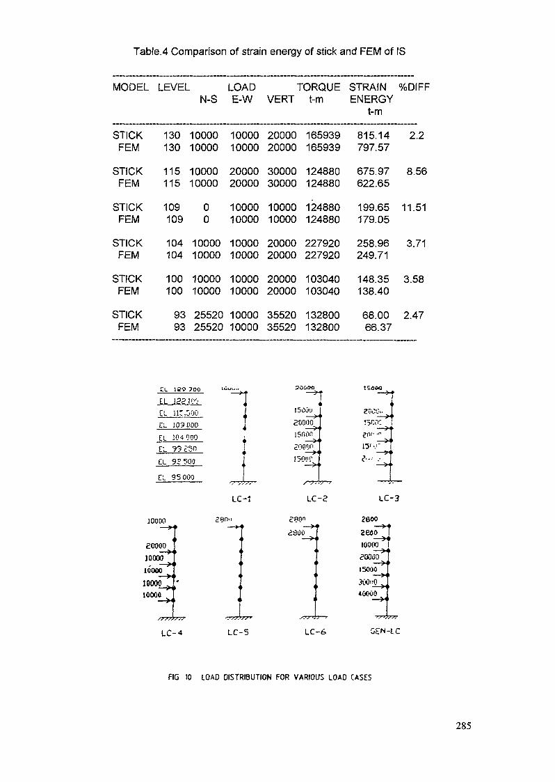
Table.4 Comparison of strain energy of stick and FEM of IS

MODEL LEVELN-S

STICK 130 10000FEM 130 10000

STICK 115 10000FEM 115 10000

STICK 109 0FEM 109 0

STICK 104 10000FEM 104 10000

STICK 100 10000FEM 100 10000

STICKFEM

CL

£LTL

93 2552093 25520

189 700 l

12210'.'ir.ooo

LOADE-W

1000010000

2000020000

1000010000

1000010000

1000010000

1000010000

•"•"""> »

D_ 109000

EL 104000

EL '?3£5n

{ \

t .

«

CL 92^00

EL 95 000

10000— »-i

20000

10000

10000. V )

10000 ?

10000

t

LC-1

cSn-ii ^*

•777-

r

1

4

77*

VERT

2000020000

3000030000

1000010000

2000020000

2000020000

3552035520

TORQUEt-m

165939165939

124880124880

124880124880

227920227920

103040103040

132800132800

JùûOft—— >•

150û'j— >

200001

c

1

—— >:oor;f5U!".S

LC-ec80n

•fc-. h

as ÛO_ y.^'

I

.'.*«•' V

STRAIN %DIFFENERGY

t-m

815.14 2.2797.57

675.97 8.56622.65

199.65 11.51179.05

258.96 3.71249.71

148.35 3.58138.40

68.00 2.4766.37

ÎSOOO— 5-»

2C'OGutsnncen(i •"

•7->

—— »<

— >• .

~-"" V-

LC-3

^eoo— >•'aeôo

— X10000

200ÜO— ><

15000

jyipi'O >|

4ÛOOO

LC-4 LC-5 LC-6 GEiN-LC

FIG 10 LOAD DISTRIBUTION FOR VARIOUS LOAD CASES

285

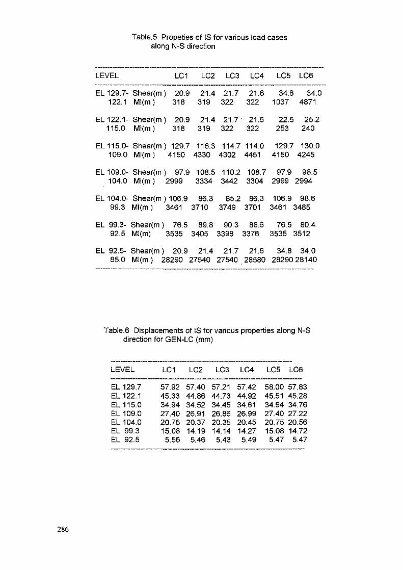
Table.5 Propeties of IS for various load casesalong N-S direction

LEVEL LC1 LC2 LC3 LC4 LC5 LC6

EL 129.7- Shear(m) 20.9 21.4 21.7 21.6 34.8 34.0122.1 Ml(m) 318 319 322 322 1037 4871

EL122.1- Shear(m) 20.9 21.4 21.7' 21.6 22.5 25.2115.0 Ml(m) 318 319 322 322 253 240

EL 115.0- Shear(m) 129.7 116.3 114.7 114.0 129.7 130.0109.0 Ml(m) 4150 4330 4302 4451 4150 4245

EL 109.0- Shear(m) 97.9 108.5 110.2 108.7 97.9 98.5104.0 Ml(m) 2999 3334 3442 3304 2999 2994

EL 104.0- Shear(m) 106.9 86.3 85.2 86.3 106.9 98.699.3 Ml(m) 3461 3710 3749 3701 3461 3485

EL 99.3- Shear(m ) 76.5 89.8 90.3 88.6 76.5 80.492.5 Ml(m) 3535 3405 3398 3376 3535 3512

EL 92.5- Shear(m) 20.9 21.4 21.7 21.6 34.8 34.085.0 Ml(m) 28290 27540 27540 28580 2829028140

Table.6 Displacements of IS for various properties along N-Sdirection for GEN-LC (mm)

LEVEL LC1 LC2 LC3 LC4 LC5 LC6ELELELELELELEL

129122115109104

.7

.1

.0

.0

.099.392.5

57.9245.3334.9427.4020.7515.085.56

574434262014

.40

.86

.52

.91

.37

.195.46

57.2144.7334.4526.8620.3514.145.43

5744.342620

.42

.92

.61

.99

.4514.275.49

58.45,34,27,20,155.

.00

.51

.94

.40

.75

.08

.47

57.8345.2834.7627.2220.5614.725.47

286

Table.7 Frequencies for various property sets (Hz)

Mode LC1 LC2 LC3 LC4 LC5 LC6

1234567

2.582.604.556.027.938.269.43

2.582.604.556.067.938.269.43

2.592.604.556.087.938.269.43

2.582.604.556.077.938.269.43

2.572.604.556.137.888.279.38

2.572.604.556.187.888.289.38

8 10.63 10.67 10.67 10.67 10.72 10.739 11.21 11.43 11.47 11.42 11.52 11.65

10 12.85 12.99 13.05 13.02 14.82 14.83

Table.8 Modal participation factors along N-S direction

Mode LC1 LC2 LC3 LC4 LC5 LC6

12345678910

39..

1.23.

3.14.2.

29011084000211978054

39122

2163

.27

.02

.02

.89

.00

.02

.08

.19

.83

.58

39.,

22.

1.17.3.

35069981000308990946

39122

2173

.40

.03

.96

.90

.00

.02

.09

.26

.09

.20

39.40 .39.011.0324.84 24.00.10.05

1.0019.32 19.67

.36

.02

.98

.77

.00

.13

.04

.63

.81

.77

6.2 Dynamic analysis of FEM and equivalent beam model

Using 3D FEM (fig.7) fequencies and participation factors are evaluatedby carrying dynamic analysis and are shown in table.9. First mode shape of3D FEM along N-S direction is shown in fig.11.

An equivalent beam model of the IS as shown in fig.7 was made forcomparing flexural modes along N-S and E-W direction. Dynamic analysis wascarried out for the two sets of properties. In one set properties derived byabove said procedure were used .(modell). In another set, propertiesobtained using classical formulae were used (model-2). Frequencies andparticipation factors for these models are given in table.9.

Similarly for calandria vault using 3D FEM (fig.8) dynamic analysis wascarried out. Frequencies and participation factors were calculated andtabulated in table. 10. First mode shapes along N-S and E-W direction areshown in fig. 12-13. Similar to the IS for CV two beam models were made anddynamic analysis was carried out. Frequencies and participation factors areshown in table. 10.

287

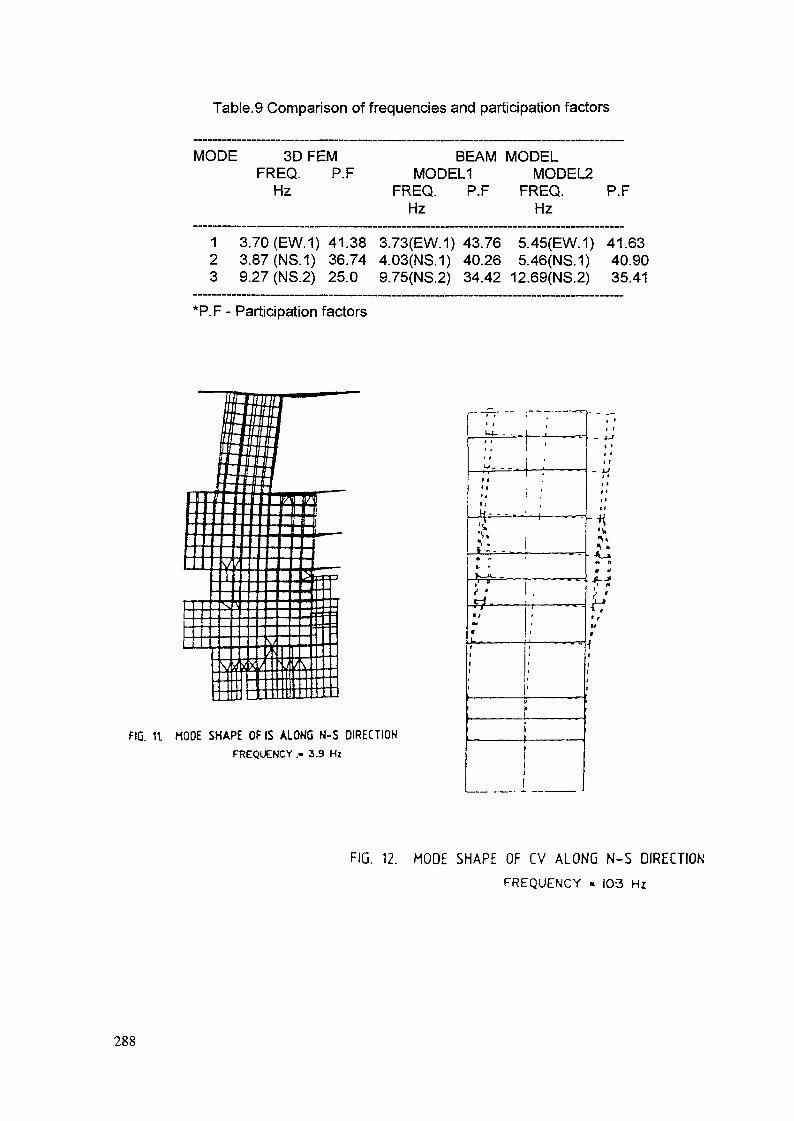
Table.9 Comparison of frequencies and participation factors

MODE 3DFEMFREQ. P.F

Hz

1 3.70 (EW.1) 41.382 3.87 (NS.1) 36.743 9.27 (NS.2) 25.0

BEAM MODELMODEL1 MODEL2

FREQ. P.F FREQ. P.FHz Hz

3.73(EW.1) 43.76 5.45(EW.1) 41.634.03(NS.1) 40.26 5.46(NS.1) 40.909.75(NS.2) 34.42 12.69(NS.2) 35.41

*P.F - Participation factors

FIG. 11 MODE SHAPE OF IS ALONG N-S DIRECTIONFREQUENCY .- 3.9 Hi

k4- - _ _' '

U_ . _

tt1

\%«,I"

•

-^ ——————t"

F?-

•/

rL(tf1

L •'1

,'

(

—i —— ^

'

1

1*

--•n<w^»*< »

A_»«• H

ff ^

?

FIG. 12. MODE SHAPE OF CV ALONG N-S DIRECTIONFREQUENCY - 103 Hz

288

FIG 13 MODE SHAPE OF CV ALONG E-W DIRECTION

FREQUENCY . 158Hi

Table. 10 Comparison of frequenciesand participation factors of CV

MODE 3DFEMFREQ. P.F

Hz

BEAM MODELMODEL1 MODEL2

FREQ. P.F FREQ. P.FHz Hz

1 10.36 (NS.1) 15.87 10.77(NS.1) 17.39 10.50(NS.1) 17 532 15.80 (EW.1) 14.99 15.82(NS.1) 18.26 14.76(EW.1) 18.45

.-7.0 DISCUSSIONS AND CONCLUSIONS

1. In the seismic analysis of RB using beam model, it is required tocalculate global response like forces and moments etc and effect of localbehaviour is neglected. Also it is required to calculate the fundamentalfrequencies more accurately. Because while generating floor response spectra(FRS) which is used for designing the equipment supported on floors, it can beobserved that the peaks will occur at the fundamental frequencies of the RB.

It can be seen from table.3 that the frequencies and participation factorsare quite different between 2D beam model and 3D beam model. In the case of2D beam model the first three frequencies are due to torsion and hence noparticipation.

2. The strain energy comparison of the system (3D FEM, 3D beam) for thegiven loading will give the idea of the stiffness comparison, because strainenergy is related to the loading and the stiffness. It can be seen from the

289

table.4 that there is a good comparison of strain energy between 3D FEM andbeam model. While calculating energy, loads are applied on the floor levelsinorder to have global deformation of the structure and neglecting localeffects. This is generally acceptable assumption.3. A comparsion of frequency of actual structure calculated by experiment orby analysis of 3D FEM with the simplified model (beam model) will give theidea of how well the stiffness and inertia effects are taken in to account whilemodelling. An excellent comparison of frequencies and participation factors canbe seen from the table.9 between 3D FEM and equivalent beam (model-A)evaluated using strain energy principle . There is a big difference infrequencies of beam model generated using classical formulas. This showsthat the classical formulas will over estimate, the stiffness. Though this will notgive much difference in response but there will be large deviation in FRS assaid before. In the higher modes the beam model ( 3D beam or 2D beam) maynot give accurate frequency and participation factors. Effect of this may beneglected because in the beam model the participation will be more than 3DFEM and give higher peaks in FRS and response of the structure.Equipments are designed by using flattened spectra. Desrepancy of higherfrequencies may not affect the design of equipment because of flatteningFRS at peaks may envelop the actual values generated by using 3D FEM. It isimportant to note that the FRS secondary peaks are smaller than the primarypeak. Hence the fundamental frequency has to be calculated as accurately aspossible.

4. If the structure is regular in shape with out any discontinuities thenclassical formulas can be adopted for calculating stiffness. This view can bestrengthened by seeing the frequencies and participation factors comparison ofcalandria vault (table. 10)

5. The stiffness of the structure should be independent of the loading setwhich will be chosen for calculating- it. Different load sets were selected.Equivalent beam properties based on energy principle were evaluated for allsets. Equivalence of these properties was established by comparingstatic displacements (table.6), frequencies (table.7) and participation factors(table.8). A good comparison of all these parameters shows that the stiffnesscalculated is independent of loading.

6. Finally it can be concluded that the method presented will eliminate theproblems of classical formulas and is simple, accurate method of modelling ofcomplex structure like Reactor Building.

290

REFERENCES

1. G.R.Reddy., R.S.Soni., B.K.Dutta., H.S.Kushwaha., A.Kakodkar. Static anddynamic analysis of nuclear containment. ASKA users conference

2. G.R.Reddy., W.V.Ramana., H.S.Kushwaha., A.Kakodkar. Seismic analysisof calandria endshield assembly of 500 MWe PHWR. RED/HSK/640/90.Reactor Engineering division, Bhabha Atomic Research Centre. Bombay-85,India.

3. Young,W.C., 1989, Roarks formulae for stress and strain. McGraw HillBook Co. Singapore.

4. ASCE 4-1986, Seismic analysis of safety related Nuclear Structures andCommentary, ASCE,345, East 47th, street, New York-10017-2398.

5. K.V.Subramanian., R.K.Ingle., H.S.Kushwaha., K.K.Vaze., G.R.Reddy.,G.V.Karandikar. Evaluation of sectional properties of a complex structure forstick model. Vol.K2, SMIRT-12,1993.

6. G.R.Reddy., K.KVaze., H.S.Kushwaha., J.V.Tandale., K.V.Subramanian.Validation of 3D beam equivalent properties obtained from FEM analysis.Internal report. Reactor Engineering Division. Bhabha Atomic Research Centre,Bombay-85, India.

291

Annex II

NON LINEAR DYNAMIC ANALYSIS INVOLVING GAPS, BUMPER SUPPORTSAND TIE RODS.

In the design of structural systems such as nuclear reactor coolant pipings,bumpers and tie rods, the basic structure is linear. For transient analysis ofpiping loops under conditions of earthquake and hypothetical accident of piperupture, the linear system becomes nonjinear because of forces due tobottoming in gaps, plastic action in bumper stops or tie rods etc. The dynamicanalysis of such structures is presented in this paper. Nonlinearities such asbumper gap elements, plasticity etc are defined as functions of motion andincorporated as generalized pseudo forces. The results of a case study ispresented and compared with the results of similar analyses reported byMOLNAR[1].

1.0 Introduction

The standard practice followed in seismic design of nuclear componentsand structures is to perform either response spectrum or response modalhistory analysis. A major part of the effort, which is common in both methods,is the solution of the eigenvalue problems. The maximum value of anyresponse of interest can be determined by using modal vectors, frequenciesand input response spectrum since for design purpose it is generallysufficient to know only the maximum value of the response. The criticisms ofthe response spectrum method arise from the fact that the phasing informationis lost in the process of evaluating the spectrum.

In time history modal analysis uncoupled equations are each numericallyintegrated using time history input function. The response quantities are thendetermined by performing time wise summation of modal responses.Response spectrum and response nodal history analysis methods are onlyvalid for linear elastic response of structure. However, the latter approachhas also been extended for nonlinear analysis of pipings. The behavior ofstructure having gaps and stops is linear during seismic event with a fewnonlinearities at support points. These nonlinearities are handled asgeneralized pseudo force. The right-hand side of the modal differentialequations and the modal superposition technique is still applicable. In thepresent case the general purpose Finite Element Program COSMOS/M version1.61 is used to carry out the analysis. A case study is presented viz. a threedimensional piping system subjected to external forces at various supports(figure 1).

2.0 Gap-Friction finite element and determination of pseudo forces

The Gap-friction element is defined by two nodes representing the distancebetween any two points in a 2D or 3D model. The gap element is defined interms of a initial gap distance and a stiffness value. The element behavessimilar to a rigid link which can resist either compression or tension in thedirection normal to the interface. A compressive gap resists compression

292

Fs (t) 10

HG. 1 A TYPICAL 3D PIPING SYSTEM WITH GAP RESTRAINTS

once the relative contraction between the two nodes exceeds the defined gapdistance. A tensile gap limits the relative expansion between the two nodes tothe gap distance. The gap-friction element is an agent which can simulate thegap forces rather than any stiffness. The so called gap stiffness which in realitymay not exist is introduced to cater the local deformation of the colliding bodiesand this stiffness is active only during the period of collision and plays no partbefore or after the collision. This stiffness doesn't affect the free vibrationcharacteristics of the initial linear structure and thus is not part of the linearstructure. For a rigid gap the gap stiffness is set to infinity. That is after theclosure of the gap any local deformation is resisted and behaves perfectlyrigid. An iterative procedure is adopted in the solution of problems involvinggap elements. The iteration is performed at the end of each time step on gapelements which are closed, to ensure convergence of the force in the elementto its correct value corresponding to the relative displacement between the twonodes. Friction forces may also be considered in conjunction with gapelements if the coefficient of friction is supplied. Sliding resistance developsonce the gap is closed. Maximum force of friction at each time step is equal tothe product of normal force Fn and the coefficient of friction..

Damper elements can also be considered between any two nodes or any onenode and ground for modal time-history problems. The damping coefficient isdefined in terms of its components along the global X,Y and Z directions.

293

3.0 Application

A three dimensional piping system has been considered along with bumpersupports as shown in the figure 1 and the response of the system due to theexternally applied forces as shown in figure 2 has been determined by modalsuperposition technique. The piping system consists of 9 pipe elements, twoelbows and three gap-bumper supports. The piping system is fixed at its ends.The model without the presence of the gap supports, represents the basic linearsystem. Tables 1,2 and 3 respectively list the properties of the pipe, propertiesof the gap-bumper supports and the nodal coordinates and inertial values.

3000-

10cO

- 2000-

C

_0"JZc

o loao-i_ob_

F,

T——I——I——I——I——I——I——I——I——I——10.4 0.5

Time in secondsFigure 2 Externally applied forces at supportsshown in figure 1

Table 1Properties of Pipe

Outside diameterWall thicknessYoung's modulusPoisson's ratio

= 508 mm= 25.4 mm= 206.8 GPa= 0.33

Table 2Properties of gap restraints

i gi(mm) ki(MN/m)

1 6.35 350.22 3.175 525.33 1.5748 262.6

294

Table 3Nodal Coordinates and inertia values

Rotary inertiaNode X(m) Y(m) Z(m) Weight(N) (mN-sq.m)

123456789101112131415

01.272.543.813.815.085.085.085.085.08

. 5.085.085.2075.085.08

0000-0.1271.272.543.815.086.356.356.356.356.356.35

0000000-0.127001.272.542.543.815.08

4224.84224.84224.88449.704224.88449.704224.84224.84224.88449.704224.80

0002869.2002869.200002869.2000

4.0 Results

Table 4 gives the first five frequencies obtained for the 3-D linear system bythe present analysis and the corresponding values obtained by MOLNAR [1].Table 5 shows the forces generated at the bumpers at different times and thecorresponding values reported by MOLNAR [1]. From table 5 it can be clearlyseen that the results of the present analysis are in excellent agreement with thatof MOLNAR [1].

Table 4Frequencies (Hz)

mode COSMOS/M MOLNAR

12345

10.3914.9516.2341.4242.06

10.3914.9416.2341.4042.04

295

Table 5Gap forces in kN

gap1 gap2 gaps

Time COSMOS/M MOLNAR COSMOS/M MOLNAR COSMOS/M MOLNAR

0.0000.0250.0500.0750.1000.1250.1500.1750.2000.225

0.0961.2

1030.1003.1348.10.9252.91686.2150.438.8

0.0961.5

1028.21003.81345.7

13.3252.21687.32153.8428.3

0.00.0

203.50.0

88.10.0

947.91247.127.2

89.5

0.00.0

203.20.0

91.60.0

947.31243.0157.9100.5

0.0417.5653.4

0.0649.5

1035.1909.1410.1243.1740.

0.0428.7654.1

0.0651.5

1033.11912.81412.51229.71754.5

0.250 1629. 1630.8 1587. 1564.1 2132. 2153.80.275 558.4 550.6 349.7 353.6 2418. 2394.90.300 0.0 0.0 50.2 56.5 2162. 2144.9

5.0 Discussion/Conclusion

The results for the natural frequencies and the gap forces obtained by thepresent analysis are in excellent agreement with the corresponding valuesreported by MOLNAR[2].

From the results of case study presented above it is concluded that complexpiping systems with nonlinear support conditions subjected to varying forcingfunctions can be easily analyzed using the gap-friction element of COSMOS/M

References

[1] Molnar A.J., Vashi K.M., and Gay C.W., "Application of Normal Modetheory and Pseudo force Methods to Solve Problems WithNonlinearities" Trans, of ASME J. of pressure vessel Technology,vol 98 May 1976.

296

SEISMIC ANALYSIS OF MONJU ANDRAPSODIE LMFBR CORE MOCK-UPS

B. FONTAINE, F. GANTENBEINCEA-CEN Saclay,Gif-sur-Yvette, France

Abstract

ABSTRACT : Sophisticated methods have been developed to study the seismic response ofLMFBR cores. These methods, mainly based on FEM beam models take into account nonlinearities and fluid structure interaction. The associated numerical techniques consistessentially in the computer code CASTEM 2000, developed by CEA/DMT. In order tovalidate these methods, a long series of experiments were performed on core mock-upsloaded by seismic excitations. Several tests, performed in air and in water ( simulatingsodium ) were applied on Rapsodie and Monju cores. The aim of this paper is to present andto compare the experimental results and calculation through assembly displacements andshock forces.

1. STATE OF THE ART REVIEW OF CEA/DMT WORK

The fast reactors are made of several hundred flexible beams embedded in a diagrid,separated by small gaps and immersed in a fluid. So to study the dynamic response of a coreto an earthquake, we need a non-linear model which takes into account the shock betweenassemblies and the fluid-structure interaction.

The shock forces are simulated by systems of non-linear springs and dampers. Thesesprings must take into account two aspects : the local stiffness of ovalisation due to localdeformation of the beam and the stiffness due to neglected modes.

The inertial effects due to fluid-structure interaction have been taken into accountthrough different ways :

• distributed mass added to assembly models : this kind of modelization has beenapplied to Rapsodie [1], Phénix and SuperPhenix cores [2],

• modelization with finite elements of fluid and structures [3],

• homogeneization : this method consists in replacing the physical heterogenousmedium ( the assemblies and the surrounding fluid ) by an homogenous equivalentmedium [4].

In order to validate these methods and to determinate some physical parameters, testswere performed on shaking tables. The main experimental programs are Rapsodie andSymphony programs [5]. The aims of these tests are principally the experimentaldetermination of the lessening of assembly frequencies due to fluid, the fluid couplingbetween assemblies, the influence of the input direction [6], and the design of an equivalentlinear model in order to introduce a core model in a reactor vessel calculation [7].

297

2. COMPUTER CODE DESCRIPTION

For this type of study, CEA/DMT has developed the computer code CASTEM 2000.The equation of motion which is used in CASTEM 2000 is the well known Bernoulli-Eulerbeam equation. In order to avoid too small integration time step which may be required in anexplicit integration scheme, CASTEM 2000 allows the use of modal analysis. The basic beamequation is projected on the eigenmodes of the beam. Then we have to calculate the modalcoefficients which are the solutions of an harmonic type equation. The generalized force inthe second member of this equation takes into account the seimic excitation and the shockforces.

3. REACTOR CORE MOCK-UPS EXPERIMENTS AND CODE VALIDATION

3.1. Rapsodie test

3.1.1. Description of the RAPSODIE core mock-up

The RAPSODIE core mock-up is presented on the figure 1. It is composed by 91 fuelassemblies located at the center of the mock-up ( 1 central and 5 rings ) surrounded by 180neutronic shield elements ( 4 rings ).

The fuel assemblies are constituted by ( fig. 2 ) :

51

PAD ———— t

HEXCAN ———

\

DIAGRID-T0-

\

ÏÏ

r^

@

——

^^

0

?•

VL

\

' |

"

tf

u=o.c

£EoCO

F" 6o

CM

fCJ

,

FIG. 1. rapsodie mock-up. FIG.2. Fuel assembly.

298

• a cylindrical spike inserted in the diagrid,

• an hexcan containing the pin bundle ( the flat to flat dimension of the hexagonalcross section is equal to 49.8 mm ).

• pads located on the hexcan at 710 mm above the upper plate of the diagrid.

There are two contact points between the diagrid and the spike. At the lower contactpoint ( sphere-cone contact ), there is no gap between the spike and the diagrid ( the weight ofthe assembly is supported there ) but at the upper one there is a small technological clearance(0.1 mm ) necessary for the insertion of the spike into the diagrid.

The neutronic shield elements ( fig. 3 ) are constituted by a steel cylinder ( diameter 48mm ) bolted on the dummy diagrid. This dummy diagrid is located at the same level as thediagrid upper plate.

FIG. 3. Neutronic shield element.

The bundle pitch of the whole mock-up is equal to 50.8 mm. The gap separating thefaces of two adjacent fuel assemblies is equal to 1 mm except at the pad level where it isreduced to 0.1 mm. The gap separating two adjacent neutronic shield elements is equal to 2.8mm except at the top where it is reduced to 0.4 mm ( a steel ring has been added at the top ofthese elements, see fig. 3). The gaps between the external fuel assemblies and the internalneutronic shield elements are equal to 1.5 mm at the pad level and 0.4 mm at the top.

The mock-up is surrounded by a stiff cylindrical vessel ( diameter : 1.1 m ) in order toperform tests in water. The vessel is assumed to be stiff enough in order to induce noamplification of the table motion ( in the seismic frequency range ).

3.1.2. Shock stiffness and structural damping

The impacts between the subassemblies are supposed to be located at the pad levelwhere the gaps are small and at the top where the displacements are important.

299

Because the subassemblies are represented with only four modes ( in the range 0 - 200Hz ), the shock stiffnesses are corrected by neglected modes stiffness.

The values of damping used for the calculations are the following :

• 3 % for all fuel assembly modes in air

• 1% for all neutronic shield element modes in air

• 5 % for all fuel assembly modes in water

• 3 % for all neutronic shield element modes in water

3.1.3. Seismic input

The time histories of the seismic accelerations of the shaking table are presented infigures 4 and 5. To limit CPU time but in keeping a representative response, time duration foranalysis will be 2.5 s, beginning at the time 0.15 s for the test in air and at the time 1.3 s forthe test in water.

FIG. 4.

3.1.4. Preliminary analysis

3RO *CCCtC»*HOH SOfttt* -

FIG. 5.

If the fuel assemblies are assumed to be pinned at their contact points with the diagrid,and the neutronic shield elements clamped on the dummy diagrid, the first eigenfrequenciesare :

• 8.13 Hz for the fuel assemblies,

• 20.7 Hz for the neutronic shield elements.

But because of the gaps which exist between the spike of the fuel assemblies and thediagrid the behavior of fuel assemblies are typically non linear and their frequencies dependon the excitation level. In figure 6 is shown the evolution of the first eigenfrequency versusthe maximal displacement at the top. In air, the frequency is close to 8 Hz for a displacementupper than 15 mm.

300

FUEL ASSEMBLY FREQUENCY8.0

7.0

' 6.0

5.0

4.0

3.0

6 « o* *

* o o o.*.*

0.000 0.010 0.020 0.030maximal displacement (m)

FIG. 6.

0.040

+ airo waier

In water, the added mass effect was introduced by lessening ( about 15 % ) the in aireigenfrequency, and by increasing the modal masses and displacements with an added massratio ( 30 % ). The steadiness of the frequency appears then at 6.8 Hz for a maximumdisplacement of 15 mm too.

3.1.5. Seismic response analysis

• In air calculation

Since the experimental responses were only measured on the central row of the mock-up, the core model used for in air calculation was the single row model ( model A ).

In figure 7 are shown the maximum and minimum assemblies top displacements versustheir position in the core. The profile of displacement obtained from calculation is very closeto the experimental one.

In figure 8 are compared the displacement time histories of the central fuel assemblyissued from calculation and tests : the calculated displacement is very similar in magnitude tothe measured one. The synchronization between the two curves is also very good. The figure9 represents the displacement of one external fuel assembly. The impacts against neutronicshield elements is responsible for the dissymmetry. The calculation is also in good agreementwith the experimental result. Concerning the neutronic shield element displacements, we canobserve in figure 10 a discrepancy between calculation and test. The reason of thisdiscrepancy is not very clear : it is possible that the contact between the element and thediagrid is not well modelized.

The profile of impact forces in the core at pad level and at top level are shown infigure 11. We can notice that the maximal values are principally located between the fuelassemblies and the neutronic shield elements. Although there exists no experimental result,the forces can be compared with calculations performed by other members of the CRP. The

301

IIQ

0.02

0.01

0.00

-o.ot

-0.02

Extreme relative displacements at the lop of the assemblieslost RAP087 in air compared to t central row cateutatJoo

O—OMix. OtoWxl

O—DI*>.C«tajli»<tl*plac<m«M•——• Mn. DMiCOTffK b) t«*b

0 1 2 3 4 5 6 7 8 9 10 11 12 13 14 15 16 17 18 19 20Assemblies

FIG. 7.

XI E-JI SB_

* - se. calculation

test

F/G. 8. FIG. 9.

5000.0

4000.0

U 3000.0<D

5

g 2000.0

1000.0

0.0

Maximum Impact forceContrai row ealcutatjon In air RAP087

FIG. 10. FIG. 11.

302

profile of forces at pad level calculated by PNC is very similar and the values of maximumforces are the same ( 1 kN ). At top level the maximum force is reached at 5 kN, i. e. higherthan at pad level because the shock springs are suffer.

• In water calculation

To take into account the fluid-structure interaction, only added mass effect was firstapplied on the assemblies, i. e. without coupling effect with the vessel. Consequently, thefrequencies were lessening and the generalized displacement qg

1 and generalized mass mg 2

were modified in the same ratio (30 %), as explained in chapter 3.1.4.

Since the water was carried with the vessel, buoyancy effects were observed on theassemblies during the tests. This phenomenon tends to decrease the effect of seismicacceleration. To modelize it, the modal displacements of the assemblies were lessening in asecond phase, in order to introduce the coupling between the assemblies and the vessel :

q water = <lair

with:qa ( = qair x 0.3 ) : contribution due to added mass effectqc: contribution due to vessel coupling effect

The participation ratio is noted

_ q water

qair

The value of qc, generally higher than qa, depends on the distance between theassemblies and the vessel, but is considerably modified by the free surface effect. In Rapsodiecase, the ratio between the generalized displacement in water and in air was fitted from testsand estimated close to 0,9 ( i. e. a little lower in water than in air ).

The results of three calculations with different participation ratios ( r\= 0.6 or 0.9 or 1 )are compared with the experimental measures in figure 10. We can notice that thedisplacements calculated with no coupling effect ( rj = 1.3 ) would certainly be much higherthan the experimental ones. When this coupling is taken into account, the magnitudes ofdisplacements issued from calculation decrease to be in better agreement with the tests.Concerning the frequency content of the assemblies responses, a little difference can beobserved between tests and calculation which shows that a more accurate value of the addedmass ratio should be applied. About neutron shield element displacements, large differencescan be observed between tests and calculation. There is presently no clear explanation for thisdiscrepancy.

1 qg = XtMU, where M is the mass matrix, X the modal shape and U a unit vector in the direction of theseismic acceleration.

2 mg = X'MX

303

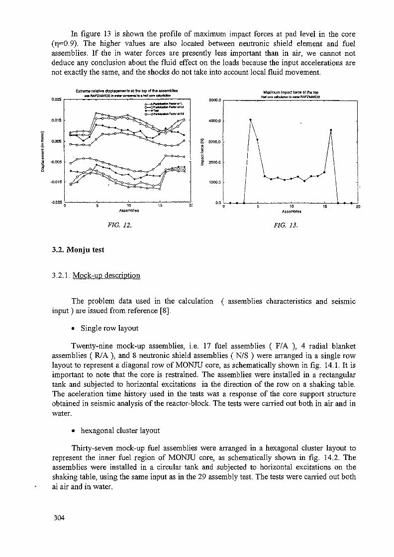
In figure 13 is shown the profile of maximum impact forces at pad level in the core(T|=0.9). The higher values are also located between neutronic shield element and fuelassemblies. If the in water forces are presently less important than in air, we cannot notdeduce any conclusion about the fluid effect on the loads because the input accelerations arenot exactly the same, and the shocks do not take into account local fluid movement.

0.025

0.015

0.005

-0.005 •

-0.015 •

-0.02S

Extrem« relativ« displacements at the top of the assembliesMl HAPZPMME3J In mur aurçna H • In» cor. nkubfcn

Maximum Impact lore« at the topH»« ox» nfcutrton h nur IWZIUME32

5 10Assemblies

FIG. 12. FIG. 13.

3.2. Monju test

3.2.1. Mock-up description

The problem data used in the calculation ( assemblies characteristics and seismicinput ) are issued from reference [8].

• Single row layout

Twenty-nine mock-up assemblies, i.e. 17 fuel assemblies ( F/A ), 4 radial blanketassemblies ( R/A ), and 8 neutronic shield assemblies ( N/S ) were arranged in a single rowlayout to represent a diagonal row of MONJU core, as schematically shown in fig. 14.1. It isimportant to note that the core is restrained. The assemblies were installed in a rectangulartank and subjected to horizontal excitations in the direction of the row on a shaking table.The aceleration time history used in the tests was a response of the core support structureobtained in seismic analysis of the reactor-block. The tests were carried out both in ah" and inwater.

• hexagonal cluster layout

Thirty-seven mock-up fuel assemblies were arranged in a hexagonal cluster layout torepresent the inner fuel region of MONJU core, as schematically shown in fig. 14.2. Theassemblies were installed in a circular tank and subjected to horizontal excitations on theshaking table, using the same input as in the 29 assembly test. The tests were carried out bothai air and in water.

304

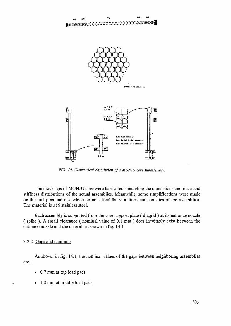
OirccttM or EiciUtiea

F/i: Fuel use«Iyt/u: blLat Dliaket Ax*e»blyH/S: tkMilran aldd iuably

F/G. 14. Geometrical description of a MONJU core subassembly.

The mock-ups of MONJU core were fabricated simulating the dimensions and mass andstiffness distributions of the actual assemblies. Meanwhile, some simplifications were madeon the fuel pins and etc. which do not affect the vibration characteristics of the assemblies.The material is 316 stainless steel.

Each assembly is supported from the core support plate ( diagrid ) at its entrance nozzle( spike ). A small clearance ( nominal value of 0.1 mm ) does inevitably exist between theentrance nozzle and the diagrid, as shown in fig. 14.1.

3.2.2. Gaps and damping

are :As shown in fig. 14.1, the nominal values of the gaps between neighboring assemblies

• 0.7 mm at top load pads

• 1.0 mm at middle load pads

305

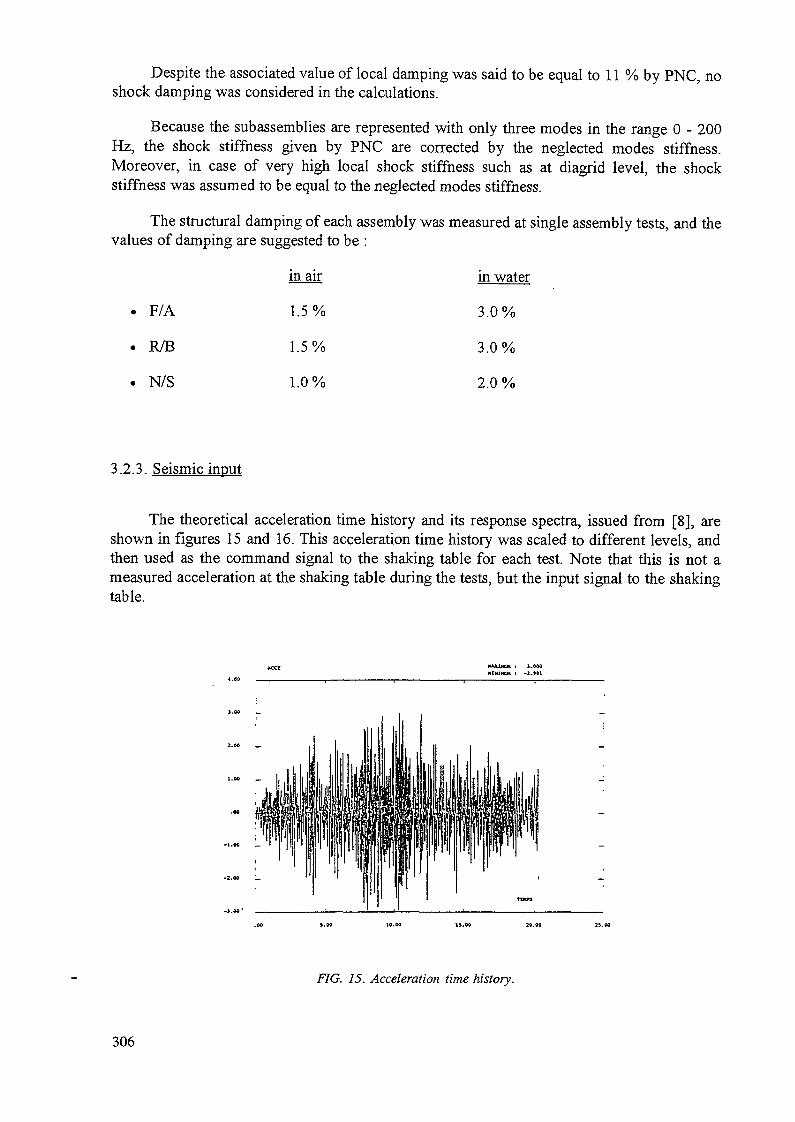
Despite the associated value of local damping was said to be equal to 11 % by PNC, noshock damping was considered in the calculations.

Because the subassemblies are represented with only three modes in the range 0 - 200Hz, the shock stiffness given by PNC are corrected by the neglected modes stiffness.Moreover, in case of very high local shock stiffness such as at diagrid level, the shockstiffness was assumed to be equal to the neglected modes stiffness.

The structural damping of each assembly was measured at single assembly tests, and thevalues of damping are suggested to be :

in water

3.0%

3.0%

2.0 %

F/A

R/B

N/S

m air

1.5%

1.5 %

1.0%

3.2.3. Seismic input

The theoretical acceleration time history and its response spectra, issued from [8], areshown in figures 15 and 16. This acceleration time history was scaled to different levels, andthen used as the command signal to the shaking table for each test. Note that this is not ameasured acceleration at the shaking table during the tests, but the input signal to the shakingtable.

MAXIMUM i 3-000XIMIHUM I -Z.ttl

FIG. 15. Acceleration time history.

306

1 I 4 < 1 3 4 t l 2 4 « 1 2 4

JOt-J IOC-1 10CO 10CI

FIG. 16. Response spectra with 1% and 1.5% damping ratio.

The excitation levels applied in this study are :

Single row layout :•0,2 g

Hexagonal cluster layout :

•0,3 g

•0,2 g•0 ,3g

'0,4g

'0,5g

3.2.4. Preliminary analysis

A linear analysis was first done to determine the in-air eigenfrequencies of theassemblies. In order to avoid the rigid body motion of the assembly due to the gaps at diagridlevel, the assembly was assumed to be pinned at this contact. The first eigenfrequenciesobtained were then :

• F/A:3.59Hz• R/B : 4.42 Hz• N/S:3.32Hz

Because of the small clearances which exist between the entrance nozzle and the coresupport plate, the frequencies of each assembly depend on the excitation level : in figure 17 isshown the evolution of the fuel first natural frequency versus the maximal displacement ofthe head. It can be noted that the asymptotic frequency is equal to 3.6 Hz and is obtained for adisplacement upper than 20 mm.

307

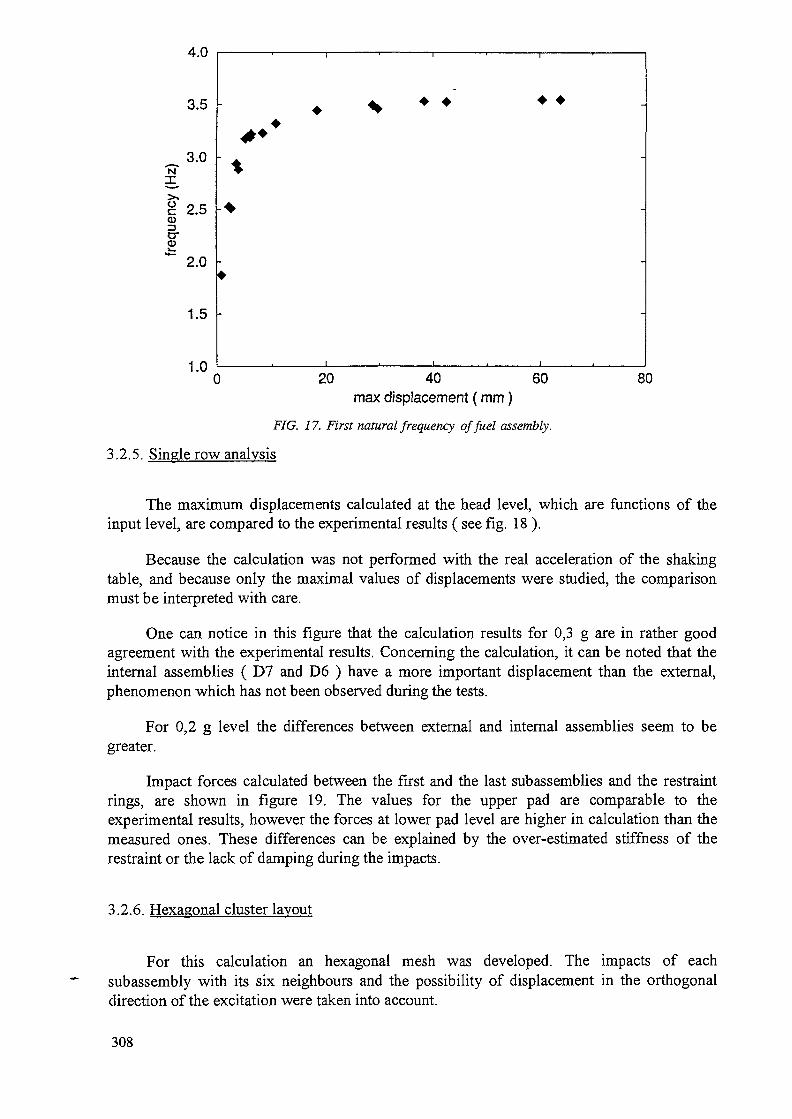
4.0

3.5

3.0

£ 2.5CD

erE*" 2.0

1.5

1.020 40 60 80

max displacement ( mm )

FIG. 17. First natural frequency offiiel assembly.

3.2.5. Single row analysis

The maximum displacements calculated at the head level, which are functions of theinput level, are compared to the experimental results ( see fig. 18 ).

Because the calculation was not performed with the real acceleration of the shakingtable, and because only the maximal values of displacements were studied, the comparisonmust be interpreted with care.

One can notice in this figure that the calculation results for 0,3 g are in rather goodagreement with the experimental results. Concerning the calculation, it can be noted that theinternal assemblies ( D7 and D6 ) have a more important displacement than the external,phenomenon which has not been observed during the tests.

For 0,2 g level the differences between external and internal assemblies seem to begreater.

Impact forces calculated between the first and the last subassemblies and the restraintrings, are shown in figure 19. The values for the upper pad are comparable to theexperimental results, however the forces at lower pad level are higher in calculation than themeasured ones. These differences can be explained by the over-estimated stiffness of therestraint or the lack of damping during the impacts.

3.2.6. Hexagonal cluster layout

For this calculation an hexagonal mesh was developed. The impacts of eachsubassembly with its six neighbours and the possibility of displacement in the orthogonaldirection of the excitation were taken into account.

308

o a o •01 02 03 Ot 05 OS 07

;

\

;

;

i A A ô A A o , ^ . ^ , .

—1—1

^ I—, --s ^> ,— «,

1 Vl/

/ © calculation

8JJL-n^rn

_

A> D

A A*0»

Ao

A

•

©t

o•*

A.D

0

©

&o,fa

©

•

O4

a

©0 0.5 0.1

input Aec. Ig]

0 - 0 1 » - Dta . 02 » - OSO - 03 » - 06

9 - 0 7

L1 »•

• • • « U

•< U

*• ; tjttff

©©

02Input Acc lg]

©© test

© calculation

FIG. 18. Single row layouts: displacements. FIG. 19. Single row layout: impact forces.

The displacements of subassemblies and impact forces against the restraint aredescribed in figures 20 and 21.

t.o

ff-ll-

^rrrff"*~~* T^

-ood. (Ton)

in >ir j

» "\

=

L3N

ÜJ

0

A1

U>

O

- L1^l

©

0

"A

f

®

O

©

o

A

/•

®

O

———— 1 ___0.1 •0.2 0.3 ' 0.4

input Ace. (g)O.S

FIG. 20. Hexagonal cluster layout: impact forces.

0.6

309

tX 1

A

OA

B

•i

8»"

©

rf

©t

e^

©

A

6

a•

©v^t

9b

D*

(D

A.

B•

^t

© a

® te

i01 02 0.3 O.i OS 0.6

Input Acc. (g)

O — No 1 101) •— No l (DO£ — No 2 (02) * — No 8 (OS)0— No3(D3) » — No 10 (06)

calculation

FIG. 21. Hexagonal cluster layout: displacements.

The agreement between calculation and experiment is rather good for thedisplacements ( see fig. 20 ). For high level ( 0.4 g and 0.5 g ), the scattering of maximumdisplacements measured during the tests is confirmed by the calculation. As for the single rowtest, the external assemblies seem to have greater displacements than the internal ones ( D4,D10).

The calculated impact forces are much higher than the measured ones. One can actuallynotice a ratio of two between the calculation and the measures ( fig. 21 ). The explanation ofthat difference may be, as for the sinle row layout, an over-estimation of the stiffness of therestraint or the lack of impact damping. Moreover, the differences between real andtheoretical acceleration can considerably modify the maximal values of impact forces.

4. CONCLUSION

CEA/DMT has performed with CASTEM 2000 calculations in order to analyse theseismic behavior of RAPSODIE and MONJU mock-ups. The aim of these calculations was todemonstrate the quality of the core models used in LMFBR core, through the determinationof shock forces between assemblies and in water behavior.

Concerning MONJU tests, calculations were performed with two layouts : single rowand hexagonal mock-up. The agreement with the test results are rather good for thedisplacements. The impact forces at upper pad level are comparable to the tests in the case ofthe single row layout but the agreement is not so good for the hexagonal cluster. In order toameliorate the results, an introduction of damping and a better estimation of stiffness of therestraint can be envisaged. Moreover, the comparison would be more accurate if the timehistories of forces and displacements were studied and not only their maximal values and ifthe calculation was performed with the real acceleration of the shaking table.

310 Next page(s) left blank

To analyse RAPSODIE tests, calculations performed with single row model and halfcore model were compared with in air and in water experimental tests. In air, the calculationresults ( maximal values and time-histories ) and measures are in rather good agreement. Inwater, there are some differences between tests and calculation when the coupling effect withthe vessel is not correctly taken into account. So the coupling mass ratio as the added massratio must be accurately estimated in order to take into account correctly the fluid-structureinteraction in FBR core calculations.

REFERENCES

[1] BROCHARD, BULAND, GANTENBEIN, GIBERT.- "Seismic analysis of LMFBRcores, mock-up RAPSODIE" - SMTRT Conference - LAUSANNE (1987) - Vol. E - pp33-42.

[2] BERNARD, VAN DORSSELAERE, GANTENBEIN.- "Seismic behavior of a fastreactor core - Application to SUPERPHENIX 1" - SMIRT Conference - CHICAGO(1983)-Paper F7/1.

[3] COMBESCURE, GIBERT, JEANPEERRE, HOFFMANN, LIVOLANT.- " Fluid-structure interaction - A general method used in the CEASEMT Computer Programs" -Computers and Structures - Vol 12, pp. 471-474 ( 1980).

[4] BROCHARD, GANTENBEIN, GIBERT.- "Dynamic analysis of LMFBR core by anhomogénéisation method" - ASME - PVP Conference - SAN DIEGO (1987).

[5] BULAND, FONTAINE, GANTENBEIN, CHERON. - "SYMPHONY experimentalmock-up" - SMIRT Conference - PORTO ALLEGRE (1995) - Paper E512 - ( to bepublished ).

[6] BROCHARD, BULAND, GANTENBEIN.- "FBR core mock-up RAPSODIE :Experimental analysis" - International Conference on Fast Reactor Core end FuelStructural Behaviour - INVERNESS ( UK) -1990.

[7] BULAND, BROCHARD.- 'Experimental determination of a LMFBR seismic equivalentcore model" - International Conference on Fast Reactor Core end Fuel StructuralBehaviour - INVERNESS ( UK) -1990.

[8] MORISHtTA - " Proposed benchmark problems from MONJU core mock-upexperiments" - IAEA/TWGFR- Coordinated reseafch program on intercomparison ofLMFBR seismic analysis codes.

Next page(s) left blank 3 j

Fontaine, B.

Horiuchi, T.

Martelli, A.(Chairman)

Morishita, M.

Rinejski, A.(Scientific Secretary)

Silaev, V.

Vaze, K.K.

LIST OF PARTICIPANTS

CEA-CEN Saclay,F-911911 Gif-sur-Yvette Cedex, France

Mechanical Engineering Laboratory,Hitachi, Ltd,502 Kandatsu,Tsuchiura, Ibaraki, 300, Japan

ENEA,Via Martiri di Monte Sole - 4,1-40129 Bologna, Italy

Systems and Components Division,Power Reactor and Nuclear Fuel Development Corporation,Oarai Engineering Center, 4002 Narita,Oarai, Ibaraki, 311-13, Japan

Division of Nuclear Power,International Atomic Energy Agency,Wagramerstrasse 5,P.O. Box 100,A-1400 Vienna, Austria

Experimental Machine Building and Design Bureau,Burnakovsky Proezd - 15,603603 Nizhny Novgorod - 74,Russian Federation

Reactor Engineering Division,Bhabha Atomic Research Centre,Trombay, Bombay 400 085, India

313