interest rate modeling in the new era - operations...
TRANSCRIPT

Interest Rate Modeling in the New Era
Fabio Mercurio
Bloomberg L.P., New York
ColumbiaMarch 21, 2016
1 / 89

Interest rates in the old eraThe pricing of a floating rate note
Before the credit crunch of 2007, interest rates in the market showedtypical textbook behavior. For instance:
Example 1A floating rate bond where LIBOR is set in advance and paid in arrearsis worth par (=100) at inception.
-0 T1 T2 TM
6
100
Ti−1 Ti
6
100 · τi · L(Ti−1,Ti)
where τi is the “length” of the interval (Ti−1,Ti], and L(Ti−1,Ti)denotes the LIBOR at Ti−1 for maturity Ti.
2 / 89

Interest rates in the old eraForward deposits vs FRAs
Example 2The forward rate implied by two deposits coincides with thecorresponding FRA rate: FDepo = FFRA.
The forward rate implied by the two deposits with maturity T1 and T2 isdefined by:
FDepo =1
T2 − T1
[P(0,T1)
P(0,T2)− 1]
The corresponding FRA rate is the (unique) value of K = FFRA forwhich the following swap(let) has zero value at time t = 0.
-
t = 0 T1 T2
L(T1,T2)− K
3 / 89

Interest rates in the old eraCompounding forward rates
Example 3Compounding two consecutive 3m forward LIBOR rates yields thecorresponding 6m forward LIBOR rate:(
1 + 14 F3m
1)(
1 + 14 F3m
2)
= 1 + 12 F6m
where
F3m1 = F(0; 3m, 6m)
F3m2 = F(0; 6m, 9m)
F6m = F(0; 3m, 9m)
-
t = 0 3m 6m 9m
︷ ︸︸ ︷︷ ︸︸ ︷︸ ︷︷ ︸
F3m1 F3m
2
F6m 4 / 89

Interest rates in the new eraThe explosion of the basis
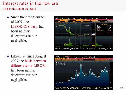
Since the credit crunchof 2007, theLIBOR-OIS basis hasbeen neitherdeterministic nornegligible.
Likewise, since August2007 the basis betweendifferent tenor LIBORshas been neitherdeterministic nornegligible.
5 / 89
Interest rates in the new eraThe explosion of the basis
Since the credit crunchof 2007, theLIBOR-OIS basis hasbeen neitherdeterministic nornegligible.
Likewise, since August2007 the basis betweendifferent tenor LIBORshas been neitherdeterministic nornegligible.
6 / 89

Interest rates in the new eraThe use of different discount and forward curves
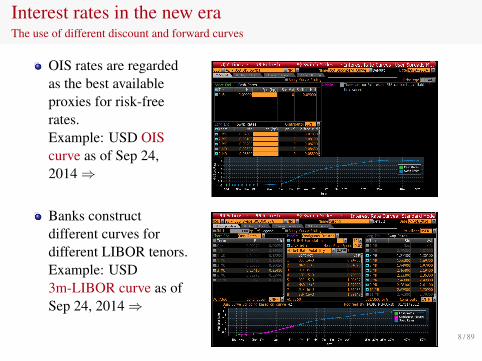
OIS rates are regardedas the best availableproxies for risk-freerates.Example: USD OIScurve as of Sep 24,2014⇒
Banks constructdifferent curves fordifferent LIBOR tenors.Example: USD3m-LIBOR curve as ofSep 24, 2014⇒
7 / 89
Interest rates in the new eraThe use of different discount and forward curves
OIS rates are regardedas the best availableproxies for risk-freerates.Example: USD OIScurve as of Sep 24,2014⇒
Banks constructdifferent curves fordifferent LIBOR tenors.Example: USD3m-LIBOR curve as ofSep 24, 2014⇒
8 / 89

Definitions in the multi-curve worldDiscount curve
We assume OIS discounting.
We consider a tenor x and an associated time structureT x = {0 < T0, . . . ,TM}, with Tk − Tk−1 = x, k = 1, . . . ,M.
OIS forward rates are defined as in the classic single-curve paradigm:
Fxk(t) := FD(t; Tk−1,Tk) =
1τk
[PD(t,Tk−1)
PD(t,Tk)− 1]
for k = 1, . . . ,M, whereτk is the year fraction for the interval (Tk−1,Tk];PD(t,T) denotes the discount factor at time t for maturity T for thediscount (OIS) curve.
Consistently with OIS discounting, we assume that risk-adjustedmeasures are defined by the discount curve.
9 / 89

Definitions in the multi-curve worldDiscount curve
We assume OIS discounting.
We consider a tenor x and an associated time structureT x = {0 < T0, . . . ,TM}, with Tk − Tk−1 = x, k = 1, . . . ,M.
OIS forward rates are defined as in the classic single-curve paradigm:
Fxk(t) := FD(t; Tk−1,Tk) =
1τk
[PD(t,Tk−1)
PD(t,Tk)− 1]
for k = 1, . . . ,M, whereτk is the year fraction for the interval (Tk−1,Tk];PD(t,T) denotes the discount factor at time t for maturity T for thediscount (OIS) curve.
Consistently with OIS discounting, we assume that risk-adjustedmeasures are defined by the discount curve.
10 / 89

Definitions in the multi-curve worldDiscount curve
We assume OIS discounting.
We consider a tenor x and an associated time structureT x = {0 < T0, . . . ,TM}, with Tk − Tk−1 = x, k = 1, . . . ,M.
OIS forward rates are defined as in the classic single-curve paradigm:
Fxk(t) := FD(t; Tk−1,Tk) =
1τk
[PD(t,Tk−1)
PD(t,Tk)− 1]
for k = 1, . . . ,M, whereτk is the year fraction for the interval (Tk−1,Tk];PD(t,T) denotes the discount factor at time t for maturity T for thediscount (OIS) curve.
Consistently with OIS discounting, we assume that risk-adjustedmeasures are defined by the discount curve.
11 / 89

Definitions in the multi-curve worldForward LIBOR rates
The forward LIBOR rate at time t for the period [Tk−1,Tk] is denotedby Lx
k(t) and defined by
Lxk(t) = ETk
D
[L(Tk−1,Tk)|Ft
],
whereL(Tk−1,Tk) denotes the LIBOR set at Tk−1 with maturity Tk;ET
D denotes expectation under the (OIS) T-forward measure;Ft denotes the “information” available at time t.
As in single-curve modeling, Lxk(t) is the fixed rate to be exchanged at
time Tk for L(Tk−1,Tk) so that the swaplet has zero value at time t:
-
t
0Value swaplet:
Time: Tk−1 Tk
L(Tk−1,Tk)− Lxk(t)
12 / 89

Definitions in the multi-curve worldForward LIBOR rates
The forward LIBOR rate at time t for the period [Tk−1,Tk] is denotedby Lx
k(t) and defined by
Lxk(t) = ETk
D
[L(Tk−1,Tk)|Ft
],
whereL(Tk−1,Tk) denotes the LIBOR set at Tk−1 with maturity Tk;ET
D denotes expectation under the (OIS) T-forward measure;Ft denotes the “information” available at time t.
As in single-curve modeling, Lxk(t) is the fixed rate to be exchanged at
time Tk for L(Tk−1,Tk) so that the swaplet has zero value at time t:
-
t
0Value swaplet:
Time: Tk−1 Tk
L(Tk−1,Tk)− Lxk(t)
13 / 89

Definitions in the multi-curve worldForward LIBOR rates
The previous definition of forward LIBOR rate is natural for the followingreasons (we omit the superscript x):
1 Lk(t) = ETkD
[L(Tk−1,Tk)|Ft
]coincides with the classically defined
forward rate in the limit case of a single curve:
ETkD
[L(Tk−1,Tk)|Ft
]= ETk
D
[FD(Tk−1; Tk−1,Tk)|Ft
]=
1τk
ETkD
[PD(t,Tk−1)−PD(t,Tk)
PD(t,Tk)
]=FD(t; Tk−1,Tk)
2 Lk(Tk−1) coincides with the LIBOR L(Tk−1,Tk):
Lk(Tk−1) = ETkD
[L(Tk−1,Tk)|FTk−1
]= L(Tk−1,Tk)
3 Lk(0) can be stripped from market data.4 Lk(t) is a martingale under the corresponding OIS forward measure5 This definition allows for a natural extension of the market formulas for
swaps, caps and swaptions.
14 / 89

Definitions in the multi-curve worldForward LIBOR rates
The previous definition of forward LIBOR rate is natural for the followingreasons (we omit the superscript x):
1 Lk(t) = ETkD
[L(Tk−1,Tk)|Ft
]coincides with the classically defined
forward rate in the limit case of a single curve:
ETkD
[L(Tk−1,Tk)|Ft
]= ETk
D
[FD(Tk−1; Tk−1,Tk)|Ft
]=
1τk
ETkD
[PD(t,Tk−1)−PD(t,Tk)
PD(t,Tk)
]=FD(t; Tk−1,Tk)
2 Lk(Tk−1) coincides with the LIBOR L(Tk−1,Tk):
Lk(Tk−1) = ETkD
[L(Tk−1,Tk)|FTk−1
]= L(Tk−1,Tk)
3 Lk(0) can be stripped from market data.4 Lk(t) is a martingale under the corresponding OIS forward measure5 This definition allows for a natural extension of the market formulas for
swaps, caps and swaptions.
15 / 89

Definitions in the multi-curve worldForward LIBOR rates
The previous definition of forward LIBOR rate is natural for the followingreasons (we omit the superscript x):
1 Lk(t) = ETkD
[L(Tk−1,Tk)|Ft
]coincides with the classically defined
forward rate in the limit case of a single curve:
ETkD
[L(Tk−1,Tk)|Ft
]= ETk
D
[FD(Tk−1; Tk−1,Tk)|Ft
]=
1τk
ETkD
[PD(t,Tk−1)−PD(t,Tk)
PD(t,Tk)
]=FD(t; Tk−1,Tk)
2 Lk(Tk−1) coincides with the LIBOR L(Tk−1,Tk):
Lk(Tk−1) = ETkD
[L(Tk−1,Tk)|FTk−1
]= L(Tk−1,Tk)
3 Lk(0) can be stripped from market data.4 Lk(t) is a martingale under the corresponding OIS forward measure5 This definition allows for a natural extension of the market formulas for
swaps, caps and swaptions.
16 / 89

Definitions in the multi-curve worldForward LIBOR rates
The previous definition of forward LIBOR rate is natural for the followingreasons (we omit the superscript x):
1 Lk(t) = ETkD
[L(Tk−1,Tk)|Ft
]coincides with the classically defined
forward rate in the limit case of a single curve:
ETkD
[L(Tk−1,Tk)|Ft
]= ETk
D
[FD(Tk−1; Tk−1,Tk)|Ft
]=
1τk
ETkD
[PD(t,Tk−1)−PD(t,Tk)
PD(t,Tk)
]=FD(t; Tk−1,Tk)
2 Lk(Tk−1) coincides with the LIBOR L(Tk−1,Tk):
Lk(Tk−1) = ETkD
[L(Tk−1,Tk)|FTk−1
]= L(Tk−1,Tk)
3 Lk(0) can be stripped from market data.
4 Lk(t) is a martingale under the corresponding OIS forward measure5 This definition allows for a natural extension of the market formulas for
swaps, caps and swaptions.
17 / 89
Definitions in the multi-curve worldForward LIBOR rates
The previous definition of forward LIBOR rate is natural for the followingreasons (we omit the superscript x):
1 Lk(t) = ETkD
[L(Tk−1,Tk)|Ft
]coincides with the classically defined
forward rate in the limit case of a single curve:
ETkD
[L(Tk−1,Tk)|Ft
]= ETk
D
[FD(Tk−1; Tk−1,Tk)|Ft
]=
1τk
ETkD
[PD(t,Tk−1)−PD(t,Tk)
PD(t,Tk)
]=FD(t; Tk−1,Tk)
2 Lk(Tk−1) coincides with the LIBOR L(Tk−1,Tk):
Lk(Tk−1) = ETkD
[L(Tk−1,Tk)|FTk−1
]= L(Tk−1,Tk)
3 Lk(0) can be stripped from market data.4 Lk(t) is a martingale under the corresponding OIS forward measure
5 This definition allows for a natural extension of the market formulas forswaps, caps and swaptions.
18 / 89

Definitions in the multi-curve worldForward LIBOR rates
The previous definition of forward LIBOR rate is natural for the followingreasons (we omit the superscript x):
1 Lk(t) = ETkD
[L(Tk−1,Tk)|Ft
]coincides with the classically defined
forward rate in the limit case of a single curve:
ETkD
[L(Tk−1,Tk)|Ft
]= ETk
D
[FD(Tk−1; Tk−1,Tk)|Ft
]=
1τk
ETkD
[PD(t,Tk−1)−PD(t,Tk)
PD(t,Tk)
]=FD(t; Tk−1,Tk)
2 Lk(Tk−1) coincides with the LIBOR L(Tk−1,Tk):
Lk(Tk−1) = ETkD
[L(Tk−1,Tk)|FTk−1
]= L(Tk−1,Tk)
3 Lk(0) can be stripped from market data.4 Lk(t) is a martingale under the corresponding OIS forward measure5 This definition allows for a natural extension of the market formulas for
swaps, caps and swaptions.19 / 89

Definitions in the multi-curve worldLIBOR-OIS basis spreads
Explicit modeling:- Additive spreads (e.g. M., 2009; Fujii et al., 2009; Amin, 2010)
Sxk (t) := Lx
k(t)− Fxk(t), k = 1, . . . ,M.
- Multiplicative spreads (e.g. Henrard, 2007, 2009)
1 + τkSxk (t) :=
1 + τkLxk(t)
1 + τkFxk(t)
, k = 1, . . . ,M.
- Instantaneous spreads (e.g. Andersen and Piterbarg, 2010)
PL(t,T) = PD(t,T) e∫ T
t s(u) du
Implicit modeling:One models the joint evolution of OIS rates and x-curve rates (e.g. M.,2010; Brace, 2010; Kenyon, 2010; Moreni and Pallavicini, 2011;Torrealba, 2011), or risk-free rates and credit events (e.g. Morini, 2012;Filipovic and Trolle, 2012).
20 / 89
Definitions in the multi-curve worldLIBOR-OIS basis spreads
Explicit modeling:- Additive spreads (e.g. M., 2009; Fujii et al., 2009; Amin, 2010)
Sxk (t) := Lx
k(t)− Fxk(t), k = 1, . . . ,M.
- Multiplicative spreads (e.g. Henrard, 2007, 2009)
1 + τkSxk (t) :=
1 + τkLxk(t)
1 + τkFxk(t)
, k = 1, . . . ,M.
- Instantaneous spreads (e.g. Andersen and Piterbarg, 2010)
PL(t,T) = PD(t,T) e∫ T
t s(u) du
Implicit modeling:One models the joint evolution of OIS rates and x-curve rates (e.g. M.,2010; Brace, 2010; Kenyon, 2010; Moreni and Pallavicini, 2011;Torrealba, 2011), or risk-free rates and credit events (e.g. Morini, 2012;Filipovic and Trolle, 2012).
21 / 89

The valuation of an interest rate swap (IRS)
We consider an IRS whose floating leg pays at Tk, k = a, . . . , b, theLIBOR with tenor Tk − Tk−1 = x, which is set (in advance) at Tk−1:
τkL(Tk−1,Tk)
The time-t value of this payoff is:
τkPD(t,Tk)ETkD
[L(Tk−1,Tk)|Ft
]= τkPD(t,Tk)Lx
k(t)
The swap’s fixed leg is assumed to pay the fixed rate K on datesT ′c, . . . ,T
′d, with year fractions τ ′j .
The IRS value to the fixed-rate payer is given by
IRS(t,K) =
b∑k=a+1
τkPD(t,Tk)Lxk(t)− K
d∑j=c+1
τ ′j PD(t,T ′j )
22 / 89

The valuation of an interest rate swap (IRS)
We consider an IRS whose floating leg pays at Tk, k = a, . . . , b, theLIBOR with tenor Tk − Tk−1 = x, which is set (in advance) at Tk−1:
τkL(Tk−1,Tk)
The time-t value of this payoff is:
τkPD(t,Tk)ETkD
[L(Tk−1,Tk)|Ft
]= τkPD(t,Tk)Lx
k(t)
The swap’s fixed leg is assumed to pay the fixed rate K on datesT ′c, . . . ,T
′d, with year fractions τ ′j .
The IRS value to the fixed-rate payer is given by
IRS(t,K) =
b∑k=a+1
τkPD(t,Tk)Lxk(t)− K
d∑j=c+1
τ ′j PD(t,T ′j )
23 / 89
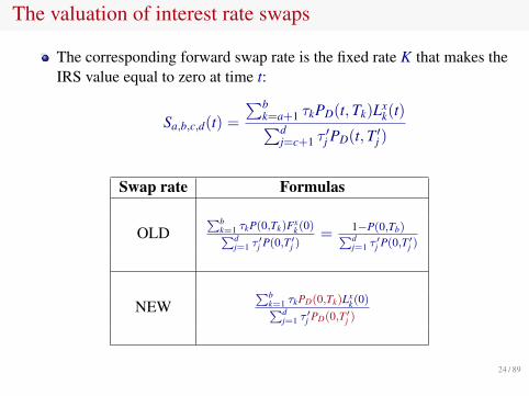
The valuation of interest rate swaps
The corresponding forward swap rate is the fixed rate K that makes theIRS value equal to zero at time t:
Sa,b,c,d(t) =
∑bk=a+1 τkPD(t,Tk)Lx
k(t)∑dj=c+1 τ
′j PD(t,T ′j )
Swap rate Formulas
OLD∑b
k=1 τkP(0,Tk)Fxk(0)∑d
j=1 τ′j P(0,T′j )
= 1−P(0,Tb)∑dj=1 τ
′j P(0,T′j )
NEW∑b
k=1 τkPD(0,Tk)Lxk(0)∑d
j=1 τ′j PD(0,T′j )
24 / 89

Dual-curve vs single-curve strippingUSD 3m forward rates
25 / 89

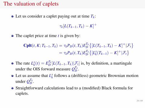
The valuation of caplets
Let us consider a caplet paying out at time Tk:
τk[L(Tk−1,Tk)− K]+
The caplet price at time t is given by:
Cplt(t,K; Tk−1,Tk) = τkPD(t,Tk)ETkD
{[L(Tk−1,Tk)− K]+|Ft
}= τkPD(t,Tk)ETk
D
{[Lx
k(Tk−1)− K]+|Ft}
The rate Lxk(t) = ETk
D [L(Tk−1,Tk)|Ft] is, by definition, a martingaleunder the OIS forward measure QTk
D .
Let us assume that Lxk follows a (driftless) geometric Brownian motion
under QTkD .
Straightforward calculations lead to a (modified) Black formula forcaplets.
26 / 89

The valuation of caplets
Let us consider a caplet paying out at time Tk:
τk[L(Tk−1,Tk)− K]+
The caplet price at time t is given by:
Cplt(t,K; Tk−1,Tk) = τkPD(t,Tk)ETkD
{[L(Tk−1,Tk)− K]+|Ft
}= τkPD(t,Tk)ETk
D
{[Lx
k(Tk−1)− K]+|Ft}
The rate Lxk(t) = ETk
D [L(Tk−1,Tk)|Ft] is, by definition, a martingaleunder the OIS forward measure QTk
D .
Let us assume that Lxk follows a (driftless) geometric Brownian motion
under QTkD .
Straightforward calculations lead to a (modified) Black formula forcaplets.
27 / 89

The valuation of caplets
Let us consider a caplet paying out at time Tk:
τk[L(Tk−1,Tk)− K]+
The caplet price at time t is given by:
Cplt(t,K; Tk−1,Tk) = τkPD(t,Tk)ETkD
{[L(Tk−1,Tk)− K]+|Ft
}= τkPD(t,Tk)ETk
D
{[Lx
k(Tk−1)− K]+|Ft}
The rate Lxk(t) = ETk
D [L(Tk−1,Tk)|Ft] is, by definition, a martingaleunder the OIS forward measure QTk
D .
Let us assume that Lxk follows a (driftless) geometric Brownian motion
under QTkD .
Straightforward calculations lead to a (modified) Black formula forcaplets.
28 / 89
The valuation of caplets
Let us consider a caplet paying out at time Tk:
τk[L(Tk−1,Tk)− K]+
The caplet price at time t is given by:
Cplt(t,K; Tk−1,Tk) = τkPD(t,Tk)ETkD
{[L(Tk−1,Tk)− K]+|Ft
}= τkPD(t,Tk)ETk
D
{[Lx
k(Tk−1)− K]+|Ft}
The rate Lxk(t) = ETk
D [L(Tk−1,Tk)|Ft] is, by definition, a martingaleunder the OIS forward measure QTk
D .
Let us assume that Lxk follows a (driftless) geometric Brownian motion
under QTkD .
Straightforward calculations lead to a (modified) Black formula forcaplets.
29 / 89

The valuation of European swaptions
A payer swaption gives the right to enter at time Ta = T ′c an IRS withpayment times for the floating and fixed legs given by Ta+1, . . . ,Tb andT ′c+1, . . . ,T
′d, respectively.
Therefore, the swaption payoff at time Ta = T ′c is
[Sa,b,c,d(Ta)− K]+d∑
j=c+1
τ ′j PD(T ′c,T′j )
where K is the fixed rate and
Sa,b,c,d(t) =
∑bk=a+1 τkPD(t,Tk)Lx
k(t)
Cc,dD (t)
Cc,dD (t) =
d∑j=c+1
τ ′j PD(t,T ′j )
30 / 89

The valuation of European swaptions
A payer swaption gives the right to enter at time Ta = T ′c an IRS withpayment times for the floating and fixed legs given by Ta+1, . . . ,Tb andT ′c+1, . . . ,T
′d, respectively.
Therefore, the swaption payoff at time Ta = T ′c is
[Sa,b,c,d(Ta)− K]+d∑
j=c+1
τ ′j PD(T ′c,T′j )
where K is the fixed rate and
Sa,b,c,d(t) =
∑bk=a+1 τkPD(t,Tk)Lx
k(t)
Cc,dD (t)
Cc,dD (t) =
d∑j=c+1
τ ′j PD(t,T ′j )
31 / 89

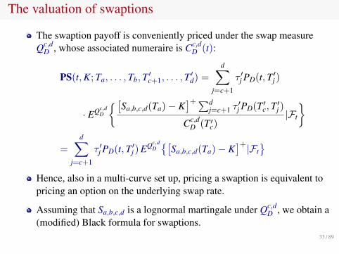
The valuation of swaptions
The swaption payoff is conveniently priced under the swap measureQc,d
D , whose associated numeraire is Cc,dD (t):
PS(t,K; Ta, . . . ,Tb,T ′c+1, . . . ,T′d) =
d∑j=c+1
τ ′j PD(t,T ′j )
· EQc,dD
{[Sa,b,c,d(Ta)− K]+∑d
j=c+1 τ′j PD(T ′c,T
′j )
Cc,dD (T ′c)
|Ft
}
=
d∑j=c+1
τ ′j PD(t,T ′j ) EQc,dD{[
Sa,b,c,d(Ta)− K]+|Ft
}
Hence, also in a multi-curve set up, pricing a swaption is equivalent topricing an option on the underlying swap rate.
Assuming that Sa,b,c,d is a lognormal martingale under Qc,dD , we obtain a
(modified) Black formula for swaptions.
32 / 89
The valuation of swaptions
The swaption payoff is conveniently priced under the swap measureQc,d
D , whose associated numeraire is Cc,dD (t):
PS(t,K; Ta, . . . ,Tb,T ′c+1, . . . ,T′d) =
d∑j=c+1
τ ′j PD(t,T ′j )
· EQc,dD
{[Sa,b,c,d(Ta)− K]+∑d
j=c+1 τ′j PD(T ′c,T
′j )
Cc,dD (T ′c)
|Ft
}
=
d∑j=c+1
τ ′j PD(t,T ′j ) EQc,dD{[
Sa,b,c,d(Ta)− K]+|Ft
}Hence, also in a multi-curve set up, pricing a swaption is equivalent topricing an option on the underlying swap rate.
Assuming that Sa,b,c,d is a lognormal martingale under Qc,dD , we obtain a
(modified) Black formula for swaptions.33 / 89

The new market formulas for caps and swaptions
Type Formulas
OLD Cplt τkP(t,Tk) Bl(K,Fx
k(t), vk√
Tk−1 − t)
NEW Cplt τkPD(t,Tk) Bl(K,Lx
k(t), v̄k√
Tk−1 − t)
OLD PS∑d
j=c+1 τ′j P(t,T ′j ) Bl
(K, SOLD(t), ν
√Ta − t
)
NEW PS∑d
j=c+1 τ′j PD(t,T ′j ) Bl
(K, SNEW(t), ν̄
√Ta − t
)
34 / 89

The new market formulas for caps and swaptionsOIS vs LIBOR discounting
USD Xy10y OIS-based swaption vols USD Xy10y LIBOR-based swaption vols
35 / 89

Pricing general interest rate derivatives
We just showed how to value swaps, caps, and swaptions under theassumption of distinct discount (OIS) and forward curves.
What about exotics?
The pricing of general interest rate derivatives should be consistent withthe practice of using OIS discounting. In fact:
A Bermudan swaption should be more expensive than the underlyingEuropean swaptions. In addition, on the last exercise date, a Bermudanswaption becomes a European swaption.A one-period ratchet is equal to a caplet.Etc ...
We must forsake the traditional single-curve models and switch to amulti-curve framework.
36 / 89

Pricing general interest rate derivatives
We just showed how to value swaps, caps, and swaptions under theassumption of distinct discount (OIS) and forward curves.
What about exotics?
The pricing of general interest rate derivatives should be consistent withthe practice of using OIS discounting. In fact:
A Bermudan swaption should be more expensive than the underlyingEuropean swaptions. In addition, on the last exercise date, a Bermudanswaption becomes a European swaption.A one-period ratchet is equal to a caplet.Etc ...
We must forsake the traditional single-curve models and switch to amulti-curve framework.
37 / 89

Pricing general interest rate derivatives
We just showed how to value swaps, caps, and swaptions under theassumption of distinct discount (OIS) and forward curves.
What about exotics?
The pricing of general interest rate derivatives should be consistent withthe practice of using OIS discounting. In fact:
A Bermudan swaption should be more expensive than the underlyingEuropean swaptions. In addition, on the last exercise date, a Bermudanswaption becomes a European swaption.A one-period ratchet is equal to a caplet.Etc ...
We must forsake the traditional single-curve models and switch to amulti-curve framework.
38 / 89

Pricing general interest rate derivatives
We just showed how to value swaps, caps, and swaptions under theassumption of distinct discount (OIS) and forward curves.
What about exotics?
The pricing of general interest rate derivatives should be consistent withthe practice of using OIS discounting. In fact:
A Bermudan swaption should be more expensive than the underlyingEuropean swaptions. In addition, on the last exercise date, a Bermudanswaption becomes a European swaption.A one-period ratchet is equal to a caplet.Etc ...
We must forsake the traditional single-curve models and switch to amulti-curve framework.
39 / 89

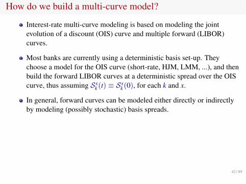
How do we build a multi-curve model?
Interest-rate multi-curve modeling is based on modeling the jointevolution of a discount (OIS) curve and multiple forward (LIBOR)curves.
Most banks are currently using a deterministic basis set-up. Theychoose a model for the OIS curve (short-rate, HJM, LMM, ...), and thenbuild the forward LIBOR curves at a deterministic spread over the OIScurve, thus assuming Sx
k (t) ≡ Sxk (0), for each k and x.
In general, forward curves can be modeled either directly or indirectlyby modeling (possibly stochastic) basis spreads.
Modeling the OIS curve is necessary for two reasons:
Swap rates depend on OIS discount factors.The pricing measures we consider are those defined by the OIS curve.
Calculating swaption prices in closed form may be hard in general.
40 / 89

How do we build a multi-curve model?
Interest-rate multi-curve modeling is based on modeling the jointevolution of a discount (OIS) curve and multiple forward (LIBOR)curves.
Most banks are currently using a deterministic basis set-up. Theychoose a model for the OIS curve (short-rate, HJM, LMM, ...), and thenbuild the forward LIBOR curves at a deterministic spread over the OIScurve, thus assuming Sx
k (t) ≡ Sxk (0), for each k and x.
In general, forward curves can be modeled either directly or indirectlyby modeling (possibly stochastic) basis spreads.
Modeling the OIS curve is necessary for two reasons:
Swap rates depend on OIS discount factors.The pricing measures we consider are those defined by the OIS curve.
Calculating swaption prices in closed form may be hard in general.
41 / 89
How do we build a multi-curve model?
Interest-rate multi-curve modeling is based on modeling the jointevolution of a discount (OIS) curve and multiple forward (LIBOR)curves.
Most banks are currently using a deterministic basis set-up. Theychoose a model for the OIS curve (short-rate, HJM, LMM, ...), and thenbuild the forward LIBOR curves at a deterministic spread over the OIScurve, thus assuming Sx
k (t) ≡ Sxk (0), for each k and x.
In general, forward curves can be modeled either directly or indirectlyby modeling (possibly stochastic) basis spreads.
Modeling the OIS curve is necessary for two reasons:
Swap rates depend on OIS discount factors.The pricing measures we consider are those defined by the OIS curve.
Calculating swaption prices in closed form may be hard in general.
42 / 89
How do we build a multi-curve model?
Interest-rate multi-curve modeling is based on modeling the jointevolution of a discount (OIS) curve and multiple forward (LIBOR)curves.
Most banks are currently using a deterministic basis set-up. Theychoose a model for the OIS curve (short-rate, HJM, LMM, ...), and thenbuild the forward LIBOR curves at a deterministic spread over the OIScurve, thus assuming Sx
k (t) ≡ Sxk (0), for each k and x.
In general, forward curves can be modeled either directly or indirectlyby modeling (possibly stochastic) basis spreads.
Modeling the OIS curve is necessary for two reasons:
Swap rates depend on OIS discount factors.The pricing measures we consider are those defined by the OIS curve.
Calculating swaption prices in closed form may be hard in general.
43 / 89

How do we build a multi-curve model?
Interest-rate multi-curve modeling is based on modeling the jointevolution of a discount (OIS) curve and multiple forward (LIBOR)curves.
Most banks are currently using a deterministic basis set-up. Theychoose a model for the OIS curve (short-rate, HJM, LMM, ...), and thenbuild the forward LIBOR curves at a deterministic spread over the OIScurve, thus assuming Sx
k (t) ≡ Sxk (0), for each k and x.
In general, forward curves can be modeled either directly or indirectlyby modeling (possibly stochastic) basis spreads.
Modeling the OIS curve is necessary for two reasons:
Swap rates depend on OIS discount factors.The pricing measures we consider are those defined by the OIS curve.
Calculating swaption prices in closed form may be hard in general.44 / 89

Deterministic basis models
In absence of market shocks, basis spreads tend to be relatively stable:
Therefore, it makes sense to assume that the LIBOR-OIS basis isconstant over time.
We consider a tenor x and an associated time structureT = {0 < T0, . . . ,TM}, with Tk − Tk−1 = x, k = 1, . . . ,M.
45 / 89

Deterministic basis models
In absence of market shocks, basis spreads tend to be relatively stable:
Therefore, it makes sense to assume that the LIBOR-OIS basis isconstant over time.
We consider a tenor x and an associated time structureT = {0 < T0, . . . ,TM}, with Tk − Tk−1 = x, k = 1, . . . ,M.
46 / 89

Deterministic basis models
In absence of market shocks, basis spreads tend to be relatively stable:
Therefore, it makes sense to assume that the LIBOR-OIS basis isconstant over time.
We consider a tenor x and an associated time structureT = {0 < T0, . . . ,TM}, with Tk − Tk−1 = x, k = 1, . . . ,M.
47 / 89

Deterministic basis models
In a deterministic and additive basis model one start by modeling OISrates.
Then one defines LIBOR rates by setting:
Lxk(t) = Fx
k(t) + Sxk (t), k = 1, . . . ,M
where, for k = 1, . . . ,M, the OIS forward rates Fxk are defined as in the
classic single-curve paradigm, namely:
Fxk(t) := FD(t; Tk−1,Tk) =
1τk
[PD(t,Tk−1)
PD(t,Tk)− 1]
and the additive basis Sxk is deterministic and given by:
Sxk (t) = Sx
k (0) = Lxk(0)− Fx
k(0)
The pricing of caps is straightforward. The pricing of swaptions ismore complex, but presents little difficulty.
48 / 89

Deterministic basis models
In a deterministic and additive basis model one start by modeling OISrates.Then one defines LIBOR rates by setting:
Lxk(t) = Fx
k(t) + Sxk (t), k = 1, . . . ,M
where, for k = 1, . . . ,M, the OIS forward rates Fxk are defined as in the
classic single-curve paradigm, namely:
Fxk(t) := FD(t; Tk−1,Tk) =
1τk
[PD(t,Tk−1)
PD(t,Tk)− 1]
and the additive basis Sxk is deterministic and given by:
Sxk (t) = Sx
k (0) = Lxk(0)− Fx
k(0)
The pricing of caps is straightforward. The pricing of swaptions ismore complex, but presents little difficulty.
49 / 89
Deterministic basis models
In a deterministic and additive basis model one start by modeling OISrates.Then one defines LIBOR rates by setting:
Lxk(t) = Fx
k(t) + Sxk (t), k = 1, . . . ,M
where, for k = 1, . . . ,M, the OIS forward rates Fxk are defined as in the
classic single-curve paradigm, namely:
Fxk(t) := FD(t; Tk−1,Tk) =
1τk
[PD(t,Tk−1)
PD(t,Tk)− 1]
and the additive basis Sxk is deterministic and given by:
Sxk (t) = Sx
k (0) = Lxk(0)− Fx
k(0)
The pricing of caps is straightforward. The pricing of swaptions ismore complex, but presents little difficulty.
50 / 89

Should one model stochastic basis spreads?
The fact that a model parameter evolves stochastically does not implythat it must be modeled as stochastic.
Do we need to model stochastic basis spreads?
Obviously, we do not have to if, for instance, we price a cap.
We clearly have to if we price an option on the LIBOR-OIS basis.
But what about non-trivial examples?Bermudan swaptionsCMS spread optionsResattable cross-currency swaptionsEUR cash-settled swaptions. . .
Stochastic-basis models can also be introduced for CVA purposes (seenext slides).
51 / 89

Should one model stochastic basis spreads?
The fact that a model parameter evolves stochastically does not implythat it must be modeled as stochastic.
Do we need to model stochastic basis spreads?
Obviously, we do not have to if, for instance, we price a cap.
We clearly have to if we price an option on the LIBOR-OIS basis.
But what about non-trivial examples?Bermudan swaptionsCMS spread optionsResattable cross-currency swaptionsEUR cash-settled swaptions. . .
Stochastic-basis models can also be introduced for CVA purposes (seenext slides).
52 / 89
Should one model stochastic basis spreads?
The fact that a model parameter evolves stochastically does not implythat it must be modeled as stochastic.
Do we need to model stochastic basis spreads?
Obviously, we do not have to if, for instance, we price a cap.
We clearly have to if we price an option on the LIBOR-OIS basis.
But what about non-trivial examples?Bermudan swaptionsCMS spread optionsResattable cross-currency swaptionsEUR cash-settled swaptions. . .
Stochastic-basis models can also be introduced for CVA purposes (seenext slides).
53 / 89
Should one model stochastic basis spreads?
The fact that a model parameter evolves stochastically does not implythat it must be modeled as stochastic.
Do we need to model stochastic basis spreads?
Obviously, we do not have to if, for instance, we price a cap.
We clearly have to if we price an option on the LIBOR-OIS basis.
But what about non-trivial examples?Bermudan swaptionsCMS spread optionsResattable cross-currency swaptionsEUR cash-settled swaptions. . .
Stochastic-basis models can also be introduced for CVA purposes (seenext slides).
54 / 89

Should one model stochastic basis spreads?
The fact that a model parameter evolves stochastically does not implythat it must be modeled as stochastic.
Do we need to model stochastic basis spreads?
Obviously, we do not have to if, for instance, we price a cap.
We clearly have to if we price an option on the LIBOR-OIS basis.
But what about non-trivial examples?Bermudan swaptionsCMS spread optionsResattable cross-currency swaptionsEUR cash-settled swaptions. . .
Stochastic-basis models can also be introduced for CVA purposes (seenext slides).
55 / 89

Should one model stochastic basis spreads?
The fact that a model parameter evolves stochastically does not implythat it must be modeled as stochastic.
Do we need to model stochastic basis spreads?
Obviously, we do not have to if, for instance, we price a cap.
We clearly have to if we price an option on the LIBOR-OIS basis.
But what about non-trivial examples?Bermudan swaptionsCMS spread optionsResattable cross-currency swaptionsEUR cash-settled swaptions. . .
Stochastic-basis models can also be introduced for CVA purposes (seenext slides).
56 / 89

An introduction to CVA
CVA stands for Credit Valuation Adjustment.
It is the adjustment to the “risk-free” value of a derivatives portfoliothat remunerates for losses upon default of counterparties.
Unilateral CVA is the CVA that focuses on counterparty’s default, andexcludes our own.
Assuming no CSA, unilateral CVA is given by:
CVA = (1− R)E[1{τ≤T}D(0, τ)V+
τ
]where
R is counterparty’s recovery rateD(0, t) is the discount factor: D(0, t) = exp{−
∫ t0 r(u) du}
τ is counterparty’s default timeVt is the portfolio value at time t
57 / 89
An introduction to CVA
CVA stands for Credit Valuation Adjustment.
It is the adjustment to the “risk-free” value of a derivatives portfoliothat remunerates for losses upon default of counterparties.
Unilateral CVA is the CVA that focuses on counterparty’s default, andexcludes our own.
Assuming no CSA, unilateral CVA is given by:
CVA = (1− R)E[1{τ≤T}D(0, τ)V+
τ
]where
R is counterparty’s recovery rateD(0, t) is the discount factor: D(0, t) = exp{−
∫ t0 r(u) du}
τ is counterparty’s default timeVt is the portfolio value at time t
58 / 89
An introduction to CVA
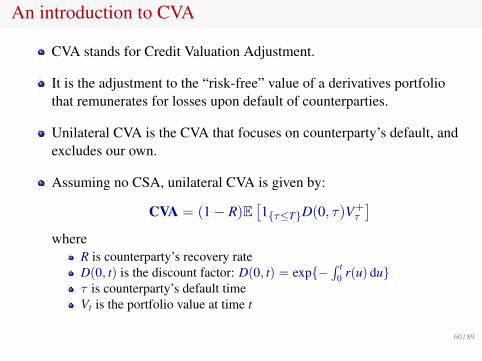
CVA stands for Credit Valuation Adjustment.
It is the adjustment to the “risk-free” value of a derivatives portfoliothat remunerates for losses upon default of counterparties.
Unilateral CVA is the CVA that focuses on counterparty’s default, andexcludes our own.
Assuming no CSA, unilateral CVA is given by:
CVA = (1− R)E[1{τ≤T}D(0, τ)V+
τ
]where
R is counterparty’s recovery rateD(0, t) is the discount factor: D(0, t) = exp{−
∫ t0 r(u) du}
τ is counterparty’s default timeVt is the portfolio value at time t
59 / 89
An introduction to CVA
CVA stands for Credit Valuation Adjustment.
It is the adjustment to the “risk-free” value of a derivatives portfoliothat remunerates for losses upon default of counterparties.
Unilateral CVA is the CVA that focuses on counterparty’s default, andexcludes our own.
Assuming no CSA, unilateral CVA is given by:
CVA = (1− R)E[1{τ≤T}D(0, τ)V+
τ
]where
R is counterparty’s recovery rateD(0, t) is the discount factor: D(0, t) = exp{−
∫ t0 r(u) du}
τ is counterparty’s default timeVt is the portfolio value at time t
60 / 89

An introduction to CVA
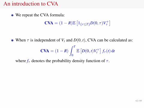
We repeat the CVA formula:
CVA = (1− R)E[1{τ≤T}D(0, τ)V+
τ
]
When τ is independent of Vt and D(0, t), CVA can be calculated as:
CVA = (1− R)
∫ T
0E[D(0, t)V+
t]
fτ (t) dt
where fτ denotes the probability density function of τ .
In general, one may want to assume a non-zero correlation between τand market risk factors, thus modeling Wrong-Way Risk (WWR). Inthis case the CVA formula becomes:
CVA = (1− R)
∫ T
0E[D(0, t)V+
t |τ = t]
fτ (t) dt
61 / 89
An introduction to CVA
We repeat the CVA formula:
CVA = (1− R)E[1{τ≤T}D(0, τ)V+
τ
]
When τ is independent of Vt and D(0, t), CVA can be calculated as:
CVA = (1− R)
∫ T
0E[D(0, t)V+
t]
fτ (t) dt
where fτ denotes the probability density function of τ .
In general, one may want to assume a non-zero correlation between τand market risk factors, thus modeling Wrong-Way Risk (WWR). Inthis case the CVA formula becomes:
CVA = (1− R)
∫ T
0E[D(0, t)V+
t |τ = t]
fτ (t) dt
62 / 89
An introduction to CVA
We repeat the CVA formula:
CVA = (1− R)E[1{τ≤T}D(0, τ)V+
τ
]
When τ is independent of Vt and D(0, t), CVA can be calculated as:
CVA = (1− R)
∫ T
0E[D(0, t)V+
t]
fτ (t) dt
where fτ denotes the probability density function of τ .
In general, one may want to assume a non-zero correlation between τand market risk factors, thus modeling Wrong-Way Risk (WWR). Inthis case the CVA formula becomes:
CVA = (1− R)
∫ T
0E[D(0, t)V+
t |τ = t]
fτ (t) dt
63 / 89

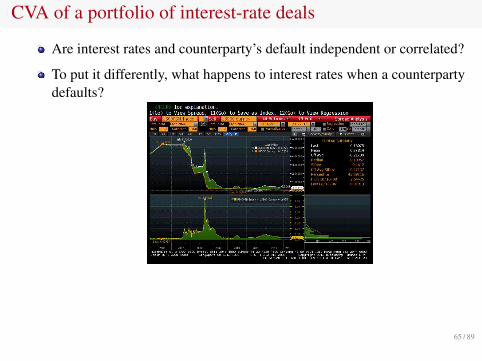
CVA of a portfolio of interest-rate deals
Are interest rates and counterparty’s default independent or correlated?
To put it differently, what happens to interest rates when a counterpartydefaults?
It appears that interest rates jump at default (of a large counterparty).
But, which rates really jump?
64 / 89
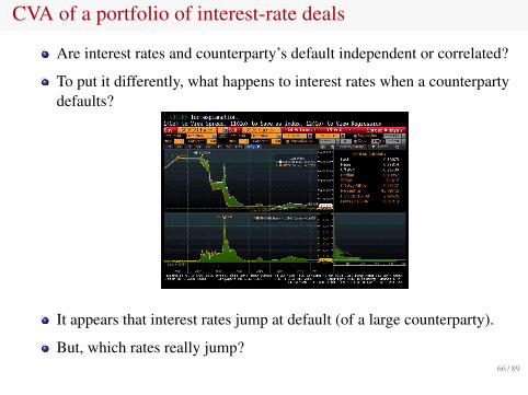
CVA of a portfolio of interest-rate deals
Are interest rates and counterparty’s default independent or correlated?
To put it differently, what happens to interest rates when a counterpartydefaults?
It appears that interest rates jump at default (of a large counterparty).
But, which rates really jump?
65 / 89
CVA of a portfolio of interest-rate deals
Are interest rates and counterparty’s default independent or correlated?
To put it differently, what happens to interest rates when a counterpartydefaults?
It appears that interest rates jump at default (of a large counterparty).
But, which rates really jump?66 / 89
Multi-curve modeling for CVA purposes
Inspired by historical evidence, M. and Li. (2015) assumed that basisspreads Sx
k (t) jump at counterparty’s default, and that they evolveaccording to:
dSxk (t) = Jx
k(t) 1{t≤τ} (−λ dt + dNt)
where N is a Poisson process with constant intensity λ.
For simplicity, we here set Jxk(t) ≡ J, so that (for t ≤ Tk−1):
Sxk (t) = Sx
k (0) +
{−λJt t < τ
−λJτ + J t ≥ τ
OIS rates can be assumed to follow any classic single-curve model.
LIBORs can then be obtained using:
Lxk(t) = Fx
k(t) + Sxk (t)
67 / 89

Multi-curve modeling for CVA purposes
Inspired by historical evidence, M. and Li. (2015) assumed that basisspreads Sx
k (t) jump at counterparty’s default, and that they evolveaccording to:
dSxk (t) = Jx
k(t) 1{t≤τ} (−λ dt + dNt)
where N is a Poisson process with constant intensity λ.
For simplicity, we here set Jxk(t) ≡ J, so that (for t ≤ Tk−1):
Sxk (t) = Sx
k (0) +
{−λJt t < τ
−λJτ + J t ≥ τ
OIS rates can be assumed to follow any classic single-curve model.
LIBORs can then be obtained using:
Lxk(t) = Fx
k(t) + Sxk (t)
68 / 89

Multi-curve modeling for CVA purposes
Inspired by historical evidence, M. and Li. (2015) assumed that basisspreads Sx
k (t) jump at counterparty’s default, and that they evolveaccording to:
dSxk (t) = Jx
k(t) 1{t≤τ} (−λ dt + dNt)
where N is a Poisson process with constant intensity λ.
For simplicity, we here set Jxk(t) ≡ J, so that (for t ≤ Tk−1):
Sxk (t) = Sx
k (0) +
{−λJt t < τ
−λJτ + J t ≥ τ
OIS rates can be assumed to follow any classic single-curve model.
LIBORs can then be obtained using:
Lxk(t) = Fx
k(t) + Sxk (t)
69 / 89
Multi-curve modeling for CVA purposes
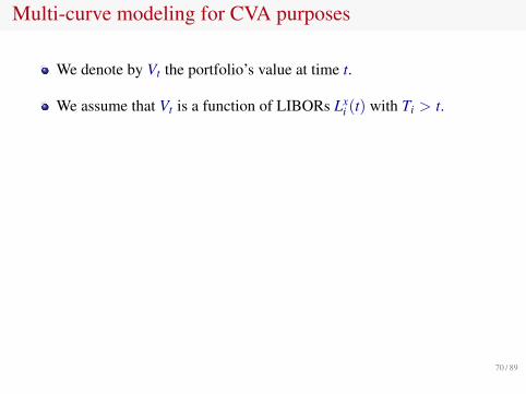
We denote by Vt the portfolio’s value at time t.
We assume that Vt is a function of LIBORs Lxi (t) with Ti > t.
For any i = 1, . . . ,M and t ≥ 0, we set:
bxi (t) :=
{Sx
i (0)− λJTi−1 if Ti−1 < tSx
i (0) + J − λJt if Ti−1 > t
which is the time-t basis conditional on default happening at time t.
We define b(t) to be the vector of all bxi (t)’s with ending date Ti > t.
Similarly, F(t) denotes the vector of forward rates Fxi (t) with Ti > t.
70 / 89

Multi-curve modeling for CVA purposes
We denote by Vt the portfolio’s value at time t.
We assume that Vt is a function of LIBORs Lxi (t) with Ti > t.
For any i = 1, . . . ,M and t ≥ 0, we set:
bxi (t) :=
{Sx
i (0)− λJTi−1 if Ti−1 < tSx
i (0) + J − λJt if Ti−1 > t
which is the time-t basis conditional on default happening at time t.
We define b(t) to be the vector of all bxi (t)’s with ending date Ti > t.
Similarly, F(t) denotes the vector of forward rates Fxi (t) with Ti > t.
71 / 89
Multi-curve modeling for CVA purposes
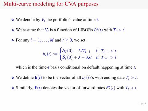
We denote by Vt the portfolio’s value at time t.
We assume that Vt is a function of LIBORs Lxi (t) with Ti > t.
For any i = 1, . . . ,M and t ≥ 0, we set:
bxi (t) :=
{Sx
i (0)− λJTi−1 if Ti−1 < tSx
i (0) + J − λJt if Ti−1 > t
which is the time-t basis conditional on default happening at time t.
We define b(t) to be the vector of all bxi (t)’s with ending date Ti > t.
Similarly, F(t) denotes the vector of forward rates Fxi (t) with Ti > t.
72 / 89

Calculating CVA for a portfolio of European-styleinterest-rate deals
With some abuse of notation, we write:
Vt = V(t,b(t),F(t)
)The WWR CVA formula is then given by
CVAWWR = (1− R)
∫ T
0E[D(0, t) V
(t,b(t),F(t)
)+]λe−λt dt
We call independent CVA the CVA obtained by setting J = 0.Denoting by B(t) the vector of initial basis spreads Sx
i (0) with Ti > t,we get
CVAIND = (1− R)
∫ T
0E[D(0, t) V
(t,B(t),F(t)
)+]λe−λt dt
73 / 89
Calculating CVA for a portfolio of European-styleinterest-rate deals
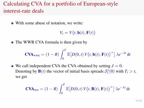
With some abuse of notation, we write:
Vt = V(t,b(t),F(t)
)The WWR CVA formula is then given by
CVAWWR = (1− R)
∫ T
0E[D(0, t) V
(t,b(t),F(t)
)+]λe−λt dt
We call independent CVA the CVA obtained by setting J = 0.Denoting by B(t) the vector of initial basis spreads Sx
i (0) with Ti > t,we get
CVAIND = (1− R)
∫ T
0E[D(0, t) V
(t,B(t),F(t)
)+]λe−λt dt
74 / 89

Calculating CVA for a portfolio of European-styleinterest-rate deals
We derive two CVA approximations by adjusting the initial basis vector.
The first approximation is based on neglecting λJ terms in vector b(t):
bxi (t) ≈
{Sx
i (0) if Ti−1 < tSx
i (0) + J if Ti−1 > t
Pretending that the prompt basis jumps as well, we get:
CVAWWR(B(0)) ≈ CVAIND(B̄(0))
whereB̄(0) = B(0) + J
So, as a rule of thumb, CVA can be obtained by shifting upwards theinitial basis curve in the independent CVA model.
75 / 89

Calculating CVA for a portfolio of European-styleinterest-rate deals
We derive two CVA approximations by adjusting the initial basis vector.The first approximation is based on neglecting λJ terms in vector b(t):
bxi (t) ≈
{Sx
i (0) if Ti−1 < tSx
i (0) + J if Ti−1 > t
Pretending that the prompt basis jumps as well, we get:
CVAWWR(B(0)) ≈ CVAIND(B̄(0))
whereB̄(0) = B(0) + J
So, as a rule of thumb, CVA can be obtained by shifting upwards theinitial basis curve in the independent CVA model.
76 / 89

Calculating CVA for a portfolio of European-styleinterest-rate deals
We derive two CVA approximations by adjusting the initial basis vector.The first approximation is based on neglecting λJ terms in vector b(t):
bxi (t) ≈
{Sx
i (0) if Ti−1 < tSx
i (0) + J if Ti−1 > t
Pretending that the prompt basis jumps as well, we get:
CVAWWR(B(0)) ≈ CVAIND(B̄(0))
whereB̄(0) = B(0) + J
So, as a rule of thumb, CVA can be obtained by shifting upwards theinitial basis curve in the independent CVA model.
77 / 89

Calculating CVA for a portfolio of European-styleinterest-rate deals
We derive two CVA approximations by adjusting the initial basis vector.The first approximation is based on neglecting λJ terms in vector b(t):
bxi (t) ≈
{Sx
i (0) if Ti−1 < tSx
i (0) + J if Ti−1 > t
Pretending that the prompt basis jumps as well, we get:
CVAWWR(B(0)) ≈ CVAIND(B̄(0))
whereB̄(0) = B(0) + J
So, as a rule of thumb, CVA can be obtained by shifting upwards theinitial basis curve in the independent CVA model.
78 / 89

Calculating CVA for a portfolio of European-styleinterest-rate deals
The above approximation does not take into account the drift correctioncoming from the compensated Poisson process.A better approximation is based on replacing the time-dependent driftterm λJt with a constant (non-zero) one.
To this end, for each basis Sxi+1(t), we define the effective default time
τ̄i+1 by
τ̄i+1 := E[τ |τ < Ti] =eλTi − 1− λTi
λ(eλTi − 1)≈ Ti
2− λT2
i
12
Our second approximation then reads as:
CVAWWR(B(0)) ≈ CVAIND(B̄(0)− λJτ̄ )
whereτ̄ := {τ̄1, . . . , τ̄M}
79 / 89

Calculating CVA for a portfolio of European-styleinterest-rate deals
The above approximation does not take into account the drift correctioncoming from the compensated Poisson process.A better approximation is based on replacing the time-dependent driftterm λJt with a constant (non-zero) one.To this end, for each basis Sx
i+1(t), we define the effective default timeτ̄i+1 by
τ̄i+1 := E[τ |τ < Ti] =eλTi − 1− λTi
λ(eλTi − 1)≈ Ti
2− λT2
i
12
Our second approximation then reads as:
CVAWWR(B(0)) ≈ CVAIND(B̄(0)− λJτ̄ )
whereτ̄ := {τ̄1, . . . , τ̄M}
80 / 89

Calculating CVA for a portfolio of European-styleinterest-rate deals
The above approximation does not take into account the drift correctioncoming from the compensated Poisson process.A better approximation is based on replacing the time-dependent driftterm λJt with a constant (non-zero) one.To this end, for each basis Sx
i+1(t), we define the effective default timeτ̄i+1 by
τ̄i+1 := E[τ |τ < Ti] =eλTi − 1− λTi
λ(eλTi − 1)≈ Ti
2− λT2
i
12
Our second approximation then reads as:
CVAWWR(B(0)) ≈ CVAIND(B̄(0)− λJτ̄ )
whereτ̄ := {τ̄1, . . . , τ̄M}
81 / 89

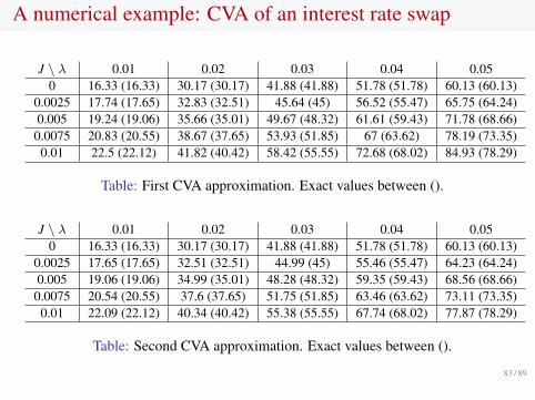
A numerical example: CVA of an interest rate swap
We consider an ATM 20-year payer interest rate swap (market data asof March 13, 2013).Features: the notional is USD 1000, the fixed rate is 2.90%, fixed-legpayments are semi-annual, floating-leg’s quarterly.We assume that the instantaneous OIS rate follows a one-factorHull-White (1990) model:
dr(t) = κ[ϑ(t)− r(t)] dt + σ dW(t)
where we set κ = 0.03 and σ = 0.005.
J \ λ 0.01 0.02 0.03 0.04 0.050 16.33 30.17 41.88 51.78 60.13
0.0025 17.65 32.51 45.00 55.47 64.240.0050 19.06 35.01 48.32 59.43 68.660.0075 20.55 37.65 51.85 63.62 73.350.0100 22.12 40.42 55.55 68.02 78.29
Table: Exact CVA. 82 / 89
A numerical example: CVA of an interest rate swap
J \ λ 0.01 0.02 0.03 0.04 0.050 16.33 (16.33) 30.17 (30.17) 41.88 (41.88) 51.78 (51.78) 60.13 (60.13)
0.0025 17.74 (17.65) 32.83 (32.51) 45.64 (45) 56.52 (55.47) 65.75 (64.24)0.005 19.24 (19.06) 35.66 (35.01) 49.67 (48.32) 61.61 (59.43) 71.78 (68.66)0.0075 20.83 (20.55) 38.67 (37.65) 53.93 (51.85) 67 (63.62) 78.19 (73.35)0.01 22.5 (22.12) 41.82 (40.42) 58.42 (55.55) 72.68 (68.02) 84.93 (78.29)
Table: First CVA approximation. Exact values between ().
J \ λ 0.01 0.02 0.03 0.04 0.050 16.33 (16.33) 30.17 (30.17) 41.88 (41.88) 51.78 (51.78) 60.13 (60.13)
0.0025 17.65 (17.65) 32.51 (32.51) 44.99 (45) 55.46 (55.47) 64.23 (64.24)0.005 19.06 (19.06) 34.99 (35.01) 48.28 (48.32) 59.35 (59.43) 68.56 (68.66)0.0075 20.54 (20.55) 37.6 (37.65) 51.75 (51.85) 63.46 (63.62) 73.11 (73.35)0.01 22.09 (22.12) 40.34 (40.42) 55.38 (55.55) 67.74 (68.02) 77.87 (78.29)
Table: Second CVA approximation. Exact values between ().
83 / 89
Conclusions
We started by describing the changes in market interest rate quoteswhich have occurred since August 2007.
We have also described the market practice of using OIS discounting inthe valuation of the main interest rate derivatives.
We have shown how to price swaps, caps and swaptions under theassumption of two distinct curves for generating future LIBOR ratesand for discounting.
The pricing formulas for caps and swaptions result in a simplemodification of the corresponding Black formulas used by the marketin the single-curve setting.
Interest rate models are then extended to the multi-curve case bymodeling basis spreads.
Finally, we have introduced a jump-at-default multi-curve model forcalculating the CVA of a portfolio of IR deals.
84 / 89

Conclusions
We started by describing the changes in market interest rate quoteswhich have occurred since August 2007.
We have also described the market practice of using OIS discounting inthe valuation of the main interest rate derivatives.
We have shown how to price swaps, caps and swaptions under theassumption of two distinct curves for generating future LIBOR ratesand for discounting.
The pricing formulas for caps and swaptions result in a simplemodification of the corresponding Black formulas used by the marketin the single-curve setting.
Interest rate models are then extended to the multi-curve case bymodeling basis spreads.
Finally, we have introduced a jump-at-default multi-curve model forcalculating the CVA of a portfolio of IR deals.
85 / 89
Conclusions
We started by describing the changes in market interest rate quoteswhich have occurred since August 2007.
We have also described the market practice of using OIS discounting inthe valuation of the main interest rate derivatives.
We have shown how to price swaps, caps and swaptions under theassumption of two distinct curves for generating future LIBOR ratesand for discounting.
The pricing formulas for caps and swaptions result in a simplemodification of the corresponding Black formulas used by the marketin the single-curve setting.
Interest rate models are then extended to the multi-curve case bymodeling basis spreads.
Finally, we have introduced a jump-at-default multi-curve model forcalculating the CVA of a portfolio of IR deals.
86 / 89
Conclusions
We started by describing the changes in market interest rate quoteswhich have occurred since August 2007.
We have also described the market practice of using OIS discounting inthe valuation of the main interest rate derivatives.
We have shown how to price swaps, caps and swaptions under theassumption of two distinct curves for generating future LIBOR ratesand for discounting.
The pricing formulas for caps and swaptions result in a simplemodification of the corresponding Black formulas used by the marketin the single-curve setting.
Interest rate models are then extended to the multi-curve case bymodeling basis spreads.
Finally, we have introduced a jump-at-default multi-curve model forcalculating the CVA of a portfolio of IR deals.
87 / 89

Conclusions
We started by describing the changes in market interest rate quoteswhich have occurred since August 2007.
We have also described the market practice of using OIS discounting inthe valuation of the main interest rate derivatives.
We have shown how to price swaps, caps and swaptions under theassumption of two distinct curves for generating future LIBOR ratesand for discounting.
The pricing formulas for caps and swaptions result in a simplemodification of the corresponding Black formulas used by the marketin the single-curve setting.
Interest rate models are then extended to the multi-curve case bymodeling basis spreads.
Finally, we have introduced a jump-at-default multi-curve model forcalculating the CVA of a portfolio of IR deals.
88 / 89

Conclusions
We started by describing the changes in market interest rate quoteswhich have occurred since August 2007.
We have also described the market practice of using OIS discounting inthe valuation of the main interest rate derivatives.
We have shown how to price swaps, caps and swaptions under theassumption of two distinct curves for generating future LIBOR ratesand for discounting.
The pricing formulas for caps and swaptions result in a simplemodification of the corresponding Black formulas used by the marketin the single-curve setting.
Interest rate models are then extended to the multi-curve case bymodeling basis spreads.
Finally, we have introduced a jump-at-default multi-curve model forcalculating the CVA of a portfolio of IR deals.
89 / 89