interfacial pattern formation in nonlinear dynamic systems: dendrites, fingers and interfacial waves...

Nonlinear Analysis. Theory, Methods % Applications, Vol. 30, No. 5, pp. 2775-2786, 1997 Proc. 2nd World Congress of Nonlinear Analysts

0 1997 Elsevier Science Ltd

PII: SO362-546X(97)00412-4 Printed in Great Britain. All rights reserved

0362.546)[/97$17.00+0.00

INTERFACIAL PATTERN FORMATION IN NONLINEAR DYNAMIC SYSTEMS:

DENDRITES, FINGERS AND INTERFACIAL WAVES BY

JIAN-JUN XU

Department of Mathematics and Statistics

McGill University

Montreal, Quebec, Canada H3A 2K6

Key words and phrases: Interfacial instabilities, pattern formation and selection, dendrite growth in solid-

ification, viscous fingering in a Hele-Shaw cell, asymptotic expansions, Stokes phenomenon.

1. INTRODUCTION

In the past several decades, two important interfacial phenomena preoccupied a large number of investigators in the broad areas of Condensed Matter Physics, Material Science, Applied Mathematics, Fluid Dynamics,

etc. (e.g. [Al-A17];[Bl-B18]). These two phenomena occur in completely different scientific fields, but both are described by similar nonlinear free boundary problem of PDE system; the boundary conditions on the in-

terface for the both cases contain a nonlinear curvature operator with the surface tension. Moreover, the both

cases raise the same theoretical issues, and they can be solved by the same analytical approach. Therefore, these two phenomena are regarded as the special examples of a variety of nonlinear phenomena in nature, and

the prominent topics of the new interdisciplinary field: nonlinear science. In what follows, we shall briefly describe these two interfacial phenomena.

Dendritic Growth in Solidification

Dendritic growth is a common interfacial phenomenon in phase transition and crystal growth. A typical single free dendrite growth is shown in Fig. 1.1.

Experimental observations show that at the later stage of growth, a dendrite has a smooth tip moving with a constant velocity. It emits a stationary wave-train, propagating along the interface towards the root. The

essence and origin of this nonlinear interfacial phenomenon have been a fundamental subject in the field of condensed matter physics and material science for a long period of time. The first important result in dendrite

growth was Ivansov’s zero surface tension, needle crystal, solution published in 1947. But the Ivantsov solution

did not solve the problem of dendrite growth. Specifically the solution cannot predict the growth rate, and being needle like, totally fails to explain the formation of microstructure visible on dendrites. The next

significant contribution was the experimental results by Schaefer, Glicksman and Ayers (1975-1976)(e.g. [A3- A4]). These researchers made extensive, detailed experiments and, on the basis of these, correctly defined the

pattern selection problem for realistic dendrite growth: the growth velocity of the dendrite tip is a uniquely determined function of the growth condition and the properties of material.

This selection problem has motivated and inspired over a generation of broad theoretical and experimental research activities.

The basic questions of dendrite growth have been: (i). what mechanism determines tip growth velocity?

(ii). what is the origin and essence of micro-structure? 2775

Second World Congress of Nonlinear Analysts 2176

(b)

Figure 1.1: Dendrite growth: (a) photograph of a single free dendrite growth from pure organic material melt Succinonitrile (SCN) (Huang and Glicksman (1981)); (b) ex p erimental record of a two dimensional dendrite growth from supersaturated (NHdBr) solution (Dougherty and Gollub (1987)).

Viscous Fingering in a Hele-Shaw Cell

Viscous fingering in Hele-Shaw cell is another famous, classic, interfacial phenomenon which occurs in the field of fluid dynamics (e.g. [Bl-B18]). The Hele-Shaw cell is a thin, essentially ‘two-dimensional’, rectangular container in which the intrusion of one fluid into another forms the commonly called ‘viscous fingers’. This

simple device has been an excellent environment for observation of fundamental features of interfacial dynamics, and the theory developed for viscous fingers provides a foundation of understanding for many fluid-fluid

systems. Observation of viscous fingers in Hele-Shaw cells has inspired over a generation of experimental and

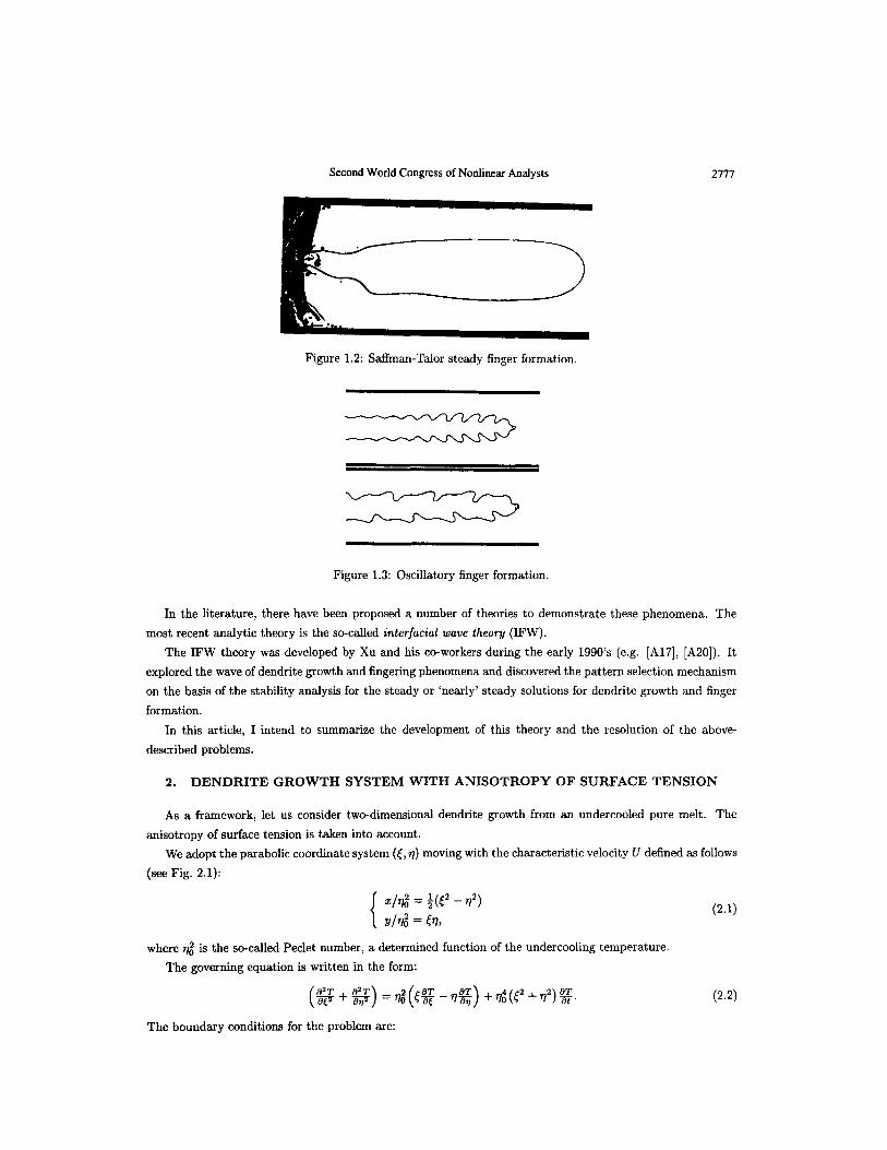
theoretical research since the first systematic study by S&man and Taylor in 1958 (e.g. [B2]). Experiments show that two types of stationary fingers can persist for long periods of time. The first type,

the subject of Saffman and Taylor’s original 1958 research, are smooth, steady fingers, which occur if the surface tension parameter is large (see Fig. 1.2). When the surface tension parameter is small, oscillatory,

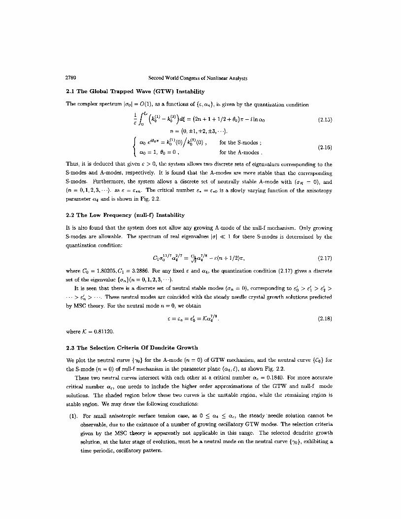
narrow, dendrite-like fingers may form. Oscillatory fingers were first discovered by Couder et. al. (1986)(e.g.

B[3]), and later, by Kopf-Sill and Homsy (1987)(e.g. [B4]). The oscillatory fingers found by Couder et. al, had a tiny bubble placed at the tip (see Fig. 1.3), while the oscillatory fingers found by Kopf-Sill and Homsy

were formed naturally without a nose bubble. The presence of even a small bubble has a noticeable effect on the finger. Of course, once the surface tension parameter is sufficiently small, stationary fingers of any kind

can no longer exist, splitting, shielding, and spreading into a chaotic pattern, throughout the Hele-Shaw cell. The fundamental issues include: (i). the stability mechanisms, (ii). the selection conditions for smooth

fingers and both types of oscillatory fingers, The above listed issues in dendrite growth and Hele-Shaw flow have been long-standing, challenging prob-

lems in the broad fields of applied mathematics, fluid mechanics, condensed matters physics, chemical engi- neering, etc. for about half a century, preoccupied many investigators from various fields.


Figure 1.2: SafFman-Talor steady finger formation.

Figure 1.3: Oscillatory finger formation.

In the literature, there have been proposed a number of theories to demonstrate these phenomena. The

most recent analytic theory is the so-called interfacial wave theory (IFW).

The IFW theory was developed by Xu and his co-workers during the early 1990’s (e.g. [A17], [A20]). It

explored the wave of dendrite growth and fingering phenomena and discovered the pattern selection mechanism

on the basis of the stability analysis for the steady or ‘nearly’ steady solutions for dendrite growth and finger

formation.

In this article, I intend to summarize the development of this theory and the resolution of the above-

described problems.

2. DENDRITE GROWTH SYSTEM WITH ANISOTROPY OF SURFACE TENSION

As a framework, let us consider two-dimensional dendrite growth from an undercooled pure melt. The

anisotropy of surface tension is taken into account.

We adopt the parabolic coordinate system (E, 7~) moving with the characteristic velocity U defined as follows

(see Fig. 2.1):

where r$ is the so-called Peclet number, a determined function of the undercooling temperature.

The governing equation is written in the form:

(2.1)

(2.2)

The boundary conditions for the problem are:

2778 Second World Congress of Nonlinear Analysts

Figure 2.1: The parabolic coordinate system used for two dimensional dendrite growth

1. The up-stream far field condition:

2. The regularity condition:

Ts = O(l), as r/ t 0;

(2.3)

(2.4)

3. The interface conditions: at 7 = n8(t, t),

(i) the thermodynamic equilibrium condition:

T = Ts (2.5)

(ii) the Gibbs-Thomson condition:

(2.6)

where s is the stability parameter of isotropic surface tension, x is the curvature operator

(2.7)

A, = f(0/(1+ t212> f(E) = (1 - a4)(1 + r2)2 + 8a,(2 (2.8)

and (~4 is the parameter of anisotropy.

(iii) the heat balance condition:

& (T - Ts) - v:& (T - Ts) + 9: (EG)

+7); (t2 + a”) % = 0 (2.9)

In addition to the above, one needs to impose the tip smooth conditions at < = 0 and the root conditions at

< = L >> 1. Given the parameters 0 5 E << 1, -1 < T, < 0 and 0 5 cr4 < 1, the above system allows the

steady state solutions, and some even more general, ‘nearly’ steady solutions. The crucial issue is the stability

of these steady, or ‘nearly’ steady solutions.


A linear eigenvalue problem for the perturbations can be formulated and is to be solved in the whole

complex < plane. Let E + 0, in terms of the multiple variables expansion (MVE) method, one can derive the eigen modes for the linear perturbed system.

These eigenmodes in the outer region can be described by some special types of traveling waves

which are subject to the following local dispersion formula:

where

Al = E&g A0 = 1

For any fixed eigenvalue oo, one can solve three wave numbers as the functions of <,

(2.10)

(2.11)

(2.12)

where we define

iw) = Jyql - i*ot)” (2.13)

m = -&(l - ihot)

Only the short wave branch, Hr - wave with the larger %{I$)} > 0 and the long wave branch, H3 - wave with the smaller IR{!$)} > 0 are physically meaningful. The Hz -wave with R{@} < 0 , must be ruled out.

Therefore the outer solution can be expressed as

) . (2.14)

It is then found that these MEV solutions have a singularity at 4 = & in the complex plane, where &

satisfies the equation: ac alto =O.

As a consequence, in order to derive a uniformly valid asymptotic solution, one must divide the complex <

plane into two regions: the outer region away from & and the inner region near &; derive the inner equation by using the proper inner variables and find the inner asymptotic solutions. Finally, one must match the outer

solution and the inner solution in the intermediate region. This procedure results in two different types of spectra of eigenvalues (TO: (i) the complex SpeCtrUm, CTO = (OR - iw); w > 0 ; (ii) the real spectrum, oo = oR.

Consequently, the system is subject to two different types of instability mechanisms:

(1) The global trapped wave (GTW) instability, induced by perturbations with a high frequency, IwI = O(1).

(2). The Low-Frequency (null-f) instability mechanism, induced by perturbations with low frequency, w 5

O(E).


2.1 The Global Trapped Wave (GTW) Instability

The complex spectrum 1001 = O(l), as a functions of {E, (YJ}, is given by the quantization condition

1 - SC E 0 Ec /$p -@))#= (2n+1+1/2+Be)7r-ilnac

n = (0, &I, f2, f3,. .).

LYO eiooa = kF)(O)/kf)(O) , for the S-modes ;

cQ=l, eo=o, for the A-modes

(2.15)

(2.16)

Thus, it is deduced that given E > 0, the system allows two discrete sets of eigenvalues corresponding to the

S-modes and A-modes, respectively. It is found that the A-modes are more stable than the corresponding

S-modes. Furthermore, the system allows a discrete set of neutrally stable A-mode with (on = 0), and

(n = 0, 1,2,3,. .). as E = Ebb. The critical number st = E*O is a slowly varying function of the anisotropy

parameter (~4 and is shown in Fig. 2.2.

2.2 The Low F’requency (null-f) Instability

It is also found that the system does not allow any growing A-mode of the null-f mechanism. Only growing

S-modes are allowable. The spectrum of real eigenvalues 1~1 < 1 for these S-modes is determined by the

quantization condition:

C~U~“~@ = $a:” - E(n + 1/2)7r, (2.17)

where Cc = 1.80205,Ci = 3.2886. For any fixed E and cr4, the quantization condition (2.17) gives a discrete

set of the eigenvaiue {o,,}(n = 0, 1,2,3, .).

It is seen that there is a discrete set of neutral stable modes (a, = 0), corresponding to E; > E; > E; >

. . > EL > . . . . These neutral modes are coincided with the steady needle crystal growth solutions predicted

by MSC theory. For the neutral mode n = 0, we obtain

E=E~=E;=Kc$‘. (2.18)

where K = 0.81120.

2.3 The Selection Criteria Of Dendrite Growth

We plot the neutral curve (70) for the A-mode (n = 0) of GTW mechanism, and the neutral curve {Cc} for

the S-mode (n = 0) of null-f mechanism in the parameter plane (crq,E), as shown Fig. 2.2.

These two neutral curves intersect with each other at a critical number a, = 0.1840. For more accurate . .

critical number LY,, one needs to include the higher order approximations of the GTW and null-f mode

solutions. The shaded region below these two curves is the unstable region, while the remaining region is

stable region. We may draw the following conclusions:

(1). For small anisotropic surface tension case, as 0 < (~4 5 a,, the steady needle solution cannot be

observable, due to the existence of a number of growing oscillatory GTW modes. The selection criteria

given by the MSC theory is apparently not applicable in this range. The selected dendrite growth

solution, at the later stage of evolution, must be a neutral mode on the neutral curve {-ye}, exhibiting a

time periodic, oscillatory pattern.


Figure 2.2: Neutral curves with (n = 0) for dendrite growth in the parameters (Q~,E) plane. The curve {-yo} is for the GTW mechanism; while {Co} is for the null-f mechanism.

(2). For large anisotropic surface tension case, as (~4 > a,, The selected dendrite growth solution must be a steady neutral mode on the neutral curve {Co}, exhibiting a time-independent smooth needle pattern.

This coincides with the selection criteria by the MSC theory.

3. VISCOUS FINGERING OF A HELE-SHAW FLOW

Viscous fingering in a Hele-Shaw cell can be mathematically formulated as a similar free boundary problem

of PDE. to that for dendrite growth. Consider the evolution of a finger developing in a Hele-Shaw cell in the positive y-direction of a moving coordinate system (2,~) fixed at the finger’s tip. The flow velocity in the

upstream far field is set to a constant U,, but the tip velocity, in general, may slowly change with time, as

t >> 1. (see Fig 3.1.)

Figure 3.1: The coordinate system for viscous finger formation.

For simplicity, we shall assume that the dynamic viscosity of the more viscous fluid is p, while the viscosity of the less viscous fluid is zero; all physical quantities have been averaged along the thickness of the cell, so that

the problem is treated as being two-dimensional. We utilize one-half of the width of the cell W as the length

scale and use the flow velocity at far field up-stream, U,, as the velocity scale; the product U,W is used as

the scale of the potential function d(z, y,t) of the absolute velocity field u(z,u, t). In terms of these scales,

ys(z, t) represents the interface’s shape, while the non-dimensional tip velocity is denoted by U. The effective width of the finger is defined as X = l/U. Moreover, we assume that for any finite time t > 0, the finger has


a finite length, with a triple point T (z = 1, y = ye) down stream. This triple point is also a stagnation point of the flow field. Thus, the general unsteady flow in a Hele-Shaw cell is described by Laplace’s equation

with the following boundary and regularity conditions:

1. the upstream far field condition:

?!Ll. !!!?!=o II= ey : @I ’ ax ’ as y-km;

2. the slipping condition on the side-walls:

a4 - = 0, ax at 2 = fl;

3. the interface conditions at s(z, y, t) = y - ys(z, t) = 0,,

(i). the dynamic condition

4 = E2n{Ys(x,t)h

(ii). the kinematic condition

Ts 2 = V, = U(t)(e, n) - fl

(3.2)

(3.3)

(3.4)

(3.5)

Here, {e,, er,} are the unit coordinate vectors along the x-axis and y-axis, respectively; n is the outward

normal vector of the interface; K is the curvature operator and the surface tension parameter is defined

as

where y is the surface tension and b is the thickness of the cell.

4. the downstream triple point condition:

04 a4 u=o: -=-=I), ax ax at z = fl, y = ylT(t);

Since the triple point T is a stagnation point, from the kinematic consideration it follows that

J

t y = yT(t) = -L - o Udt.

5. the regularity conditions at the tip.

(3.6)

(3.7)

(3.8)

Given parameters 0 5 E (< 1 and 0 < X = l/U < 1, this system may not allow the steady finger solution, but it does allows a class of the ‘nearly’ steady finger solutions. The crucial issue again is the stability of these ‘nearly’ steady finger solutions.


Very similar to the case of dendrite growth, one can derive the eigen modes for the linear perturbed system

in terms of the multiple variables expansion (MVE) method. These eigen modes, in the outer region, are also

described by some travelling waves expressed in the form

ho = Lo(p) = D exp { $ + i lp kc&),

where p is a new variable measuring the arc length of the interface of the finger staring from the tip. These

waves are subject to a similar local dispersion formula:

uo = C*(p,io) = g.$ [(I - @) - E&Y@] . 0 0

This formula can be written in the form, exactly as for dendrite growth:

me = -G,b) = s(p)2 Jf.- [(l - ip) - &]

(3.10)

(3.11)

provided one sets

k e

= G(P)ko; (T, = x312

AU2 0 00. (3.12) 0

The outer solutions

~o=Dl~xp{~+~~P~~‘d~),Daexp{~+~~~~~’dp}~ (3.13)

also has a singular point pc in the complex plane. Hence, the similar matching procedure is also needed. It

leads to a very similar spectra structure: (i) the complex spectrum oo = (un - iw); w > 0 and (ii) the real

spectrum. Accordingly, the system is also subject to the instability mechanisms:

(1). The global trapped wave (GTW) instability, induced by perturbations with a high frequency, Iwl = O(1).

(2). The Low-Frequency (null-f) instability mechanism, induced by perturbations with low frequency, w =

O(E).

3.1 The GTW Instability

For the complex spectrum, we obtain the following quantization conditions:

1 - /( E 0

Pc $’ - if’)+ = (2n + 1 + l/2 + .!&)a - ilncuo (3.14)

n = (0, fl, f2, ~t3,. . .),

where

This quantization condition determines two discrete sets of complex eigenvalues for S-modes and A-modes,

respectively, as the functions of (E, X0). Given Xo, the system allows a set of neutrally stable modes (on = 0),

as E = .sen, (n = 0, 1,2,. . .), where E*O = E, > ~~1 > ~~2 > . . Or given E, the system allows a set of neutrally

stable modes with Xo = Xl;‘, (n = 0, 1,2,. .), where Xr’ < Xt’ < . . . It has been found that the neutral

A-modes are more stable than the neutral S-modes. The neutral A-mode (n=O) curve is shown in Fig. 3.2.


3.2 The Null-f Instability

For the null-f instability, it is found that the S-modes are more stable than the corresponding A-modes. The

spectrum of the real eigenvalues oo for the S-modes is given by the quantization condition:

;xocTo = (2X0 - 1)3/4 xv2 - &(n. + 1/2)rr

0

For any fIxed E and Xo , from the quantization condition (3.16), one can obtain a discrete set of eigenvalues

{o~)}(n = 0, 1,2,3,. . .). Given Xo, the system allows a discrete set of neutral stable modes (gc’ = 0),

corresponding to E = EL, (n = 1,2,. .), where eb > E: > E; > . . > EL > ‘. . . On the other hand, given E > 0,

the system allows a discrete set of neutral modes with width parameters Xo = Xg’, or tip velocity Ue = Uin).

The neutral S-modes are determined by the formula:

(244 - 1)3i4

If-- xp

= &(n. + l/2)71 (3.17)

These neutral modes are steady finger solutions that coincide with the classic steady finger solutions discov-

ered numerically by Vanden Broeck (1983) and the MSC theory. The null-f instability was first discovered

numerically by Kessler and Levine (1986). It was also studied by Bensimon Pelce and Shraiman in terms of a

different approach (1987).

3.3 The Selection Criteria Of Finger Solutions

Based on the understanding of instability mechanisms clarified in the preceding sections, the selection criteria

for finger solutions can be naturally derived. In Fig. 3.2, we plot the neutral curve {-yo} of the A-modes

(n = 0) of the GTW mechanism, and the neutral curve {Co} the S-modes (n = 0) of the null-f mechanism, in

the parameter plane (A,&). These two neutral curves intersect with each other at a critical number cc = 0.0908.

The shaded region below these two curves is the stable region, while the region above both these two curves,

is the unstable region.

&

Figure 3.2: Neutral curves with (n = 0) for fingering formation in, the parameters (E, Xo) plane. The curve

(70) is for the GTW mechanism; while {CO} is for the null-f mechanism.

For a given operating condition, E is fixed, but X(q corresponding to the finger under the investigation may

vary. Hence, the state of our dynamical system moves slowly in the (E, X) phase plane. In general, as t + 00,

the finger solution may have the following three possible behaviors: (i) it may approach a steady solution


describing a smooth finger; (ii) it may approach a time periodic solution describing an oscillatory finger; (iii)

it may have no limiting solution, or evolves with multiple short time scales, describing a chaotic pattern.

Therefore, from the above stability analysis, one may make the following statements:

1. When E > cc, the system will have a steady limiting solution as t -+ ~0. No oscillatory finger can

persist. Such a selected steady smooth finger solution must be on the neutral curve {Cc,}. This criteria

is consistent with the microscopic solvability condition (MSC) theory.

2. However, for small surface tension, when E < cc, the steady needle solution can never persist, due to the

existence of GTW instability. Apparently, the conclusion made by Tanveer and others that the steady

finger solution (n = 0) is linearly stable for the whole range of 0 < E << 1 is incorrect and the selection

criteria given by the MSC theory is not applicable in the range 0 5 E < E,.

3. If the finger system exhibits a time periodic, oscillatory pattern as t -+ 03, this limit solution must be a

neutral mode on the neutral curve (7s) and it occurs only when 0 5 E 5 E,. The unsteady oscillatory

pattern determined by the GTW neutral mode is self-sustained. It can be stimulated by an imposed

initial perturbation and does not need a continuously acting noise for its persistence. Of course, this

criteria for the range of (E < Q) is only a necessary condition for the occurrence of a time periodic,

oscillatory finger. It has not been proved as a sufficient condition for such linear neutrally stable mode

to be actually observed. In the practice, the oscillatory fingers are easily observed, when a tiny bubble is

applied on the tip. It has been verified that the experimental date of these oscillatory fingers are indeed

on the GTW neutral curve (7s) (see [BlS]).

4. If the finger system exhibits a chaotic pattern as t + co, the state point of the system must be staying

in the unstable region.

REFERENCES

(A). Dendrite growth

Al. Ivantsov, G. P., Dokl. Akad. Nauk, SSSR.. 58, p. 567, (1947).

A2. Nash, G. E. and Glicksman, M. E., Acta Metall. 22, p. 1283, (1974).

A3. Glicksman, M. E., Schaefer, R. J. and Ayers, J. D., Phil. Mag., 32, p. 725, (1975).

A4. Glicksman, M. E., Schaefer, R. J. and Ayers, J. D., Metall. Trans., A 7, p. 1747, (1976).

A5. Langer, J. S. and Milller-Krumbaar, Acta Metall., 26, p. 1681; 1689; 1697, (1978).

A6. Langer, J. S., Rev. Mod. Phys. Vol. 52, No: 1, January (1980).

A7. Huang, S. C. and Glicksman, M. E., Acta Metall., 29, p. 701, (1981)

AB. Kessler, D. A., Koplik, J. and Levine, H., Pattern Formation Far horn Equilibrium: the free space

dendritic crystal in “Proc. NATO A.R.W. on Patterns, Defects and Microstructures in Non-equilibrium

Systems” (Astin, TX., March, 1986)

A9. Kessler, D. A. and Levine, H., Phys. Rev. Lett., 57, p. 3069, (1986).

AlO. Dougherty, A. and Gollub, J. P., The Phys. Rev. A., 38, p. 3043, (1988)

All. J.J. Xu, “Global Asymptotic Solution For Axisymmetric Dendrite Growth with Small Undercooling”

NATO AS1 Series E: Applied Science - No: 125 p. 95-109 (1987)


A12. P. Pelce,“Dynamics of Curved Front”, Academic New York, (1988)

A13. J.J. Xu, “Global Neutral Stable State and Selection Condition of Tip Growth Velocity”, J. Crystal

Growth, 100, p. 481, (1990).

A14. J.J. Xu, “Asymptotic Theory of Steady Axisymmetric Needle-like Crystal Growth”, Studies in Applied

Mathematics, 82, p. 71, (1990).

A15. J.J. Xu, “Interfacial Wave Theory of Solidification - Dendritic Pattern Formation and Selection of

Tip Velocity”, The Physical Review A 15., Vol. 43, No: 2, p. 930-947, (1991).

A16. J.J. Xu, “Two-Dimensional Dendritic Growth with Anisotropy of Surface Tension”, Physics (D), 51, p.

579-595, (1991).

A17. J.J. Xu, “Generalized Needle Solutions, Interfacial Instabilities, and Pattern Formation”, The Physical

Review E. Vol. 53, No: 5, p. 5051-5062, (1996).

(B). Viscous Fingering

Bl. Zhuravlev, PA, Zap Leningr. Corn. Inst. Vol. 33, p. 54-61 (1956).

B2. P.G. Saffman and G.I. Taylor, ProcR. Sot. London Ser. A. 245, p. 312, (1958).

B3. Y. Couder, N. Gerard and M. Rabaud, Phys. Rev. A. 34, p. 5175, (1986).

B4. A.R. Kopf-Sill and G.M. Homsy, Phys. Fluids, 30, No: 9, p. 2607, (1987).

B5. D. Bensimon, P. Pelce and B.I. Shraiman, J. Physique 48, p. 2081, (1987).

B6. Jean-Marc Vanden-Broeck, Phys. Fluids, Vol. 26, No:8, p. 2033, (1983).

B7. S. Tanveer, Phys. Fluid 30, (8), p. 1589, (1987).

B8. D.C. Hong and J.S. Langer, Phys. Rev. Lett. 56, p. 2032), (1986).

B9. D.A. Kessler and H. Levine, Phys. Rev. A, 32, p. 1930, (1985); 33, p. 2632, (1986).

BlO. J. Mclean and P.G. Saffman, J. Fluid Mech. 102, p. 455, (1981).

Bll. A.J. DeGregoria and L.W. Schwartz, J. Fluid Mech. 164, p. 383, (1986).

B12. E. Meiburg and G.M. Homsy, Phys. Fluids 31, (3), p. 429, (1988).

B13. P. Tabling, G. Zocchi and A. Libchaber, J. Fluid Mech. 177, p. 67, (1987).

B14. G.M. Homsy, Annu. Rev. Fluid Mech. 19, p. 271, (1987).

B15. S.D. Howison, A.A. Lacey and J.R. Ockendon, Q.J. Mech. Appl. Math. 41 p. 183, (1988).

B16. J.J. Xu, “Global Instability of Viscous Fingering in Hele-Shaw Cell - Formation of Oscillatory Finger-

s”, European Journal of Applied Mathematics, Vol. 2, p. 105-132, (1991).

B17. J.J. Xu, “Interfacial Wave Theory for Oscillatory Finger’s Formation in a Hele-Shaw Cell: a Comparison

with Experiments” European Journal of Applied Mathematics, Vol. 7, p. 169-199, (1996).

B18. J.J. Xu, “Interfacial Instabilities and Fingering Formation in Hele-Shaw Flow”, IMA Journal of Applied

Mathematics, 57, p. 101-135, (1996).

interfacial pattern formation in nonlinear dynamic systems: dendrites, fingers and interfacial waves...

Documents