Intergenerational health correlations: Is it genes or is it

income?

Ana Llena-Nozal

a*

Maarten Lindeboom b

Bas van der Klaauw c

January 2006

Very preliminary and incomplete

Abstract: This paper investigates how much of health is transmitted across generations through

genetics and how much through behavior and socio-economic status (SES). Low SES children

start adulthood with lower education and health and this may constrain their economic position in

adulthood. The intergenerational correlation of income may be linked to health but it is not clear

what mechanisms are driving this. Low SES parents may face financial constraints that lower

parental investment, they may have lower parenting skills, or they may have worse health

outcomes that constraint economic opportunities and these may be transmitted across generations.

Both unobserved heterogeneity and parental health need to be accounted for in order to

disentangle the correlation. We use a cohort study, the National Child Development Study, which

follows individuals since their birth in 1958 until their 40s. We exploit the richness of the data

and incorporate information on twins, adoptees and the cohort members’ own children to

disentangle the nature and nurture components. Our findings suggest that parental income

significantly reduces the risk of ill health in children. Individuals not having a natural father are

more prone to poor health but experience a similar mitigating impact of income. Income appears

to no longer be significant when we control for parental health and time investment. On the other

hand, when financial difficulties are used to measure poverty, the effects persist, even after

controlling for individual unobserved heterogeneity.

a: Free University Amsterdam & Tinbergen Institute.

b. Free University Amsterdam, Tinbergen Institute, HEB, IZA & Netspar.

* Correspondence: Department of Economics and Business Administration, Free University of Amsterdam,

De Boelelaan 1105, 1081 HV Amsterdam, The Netherlands. E-mail: allenanozal@econ.vu.nl

c. Free University Amsterdam, Tinbergen Institute, Scholar & CEPR.

1. Introduction

There exists a strong positive association between health and socio-economic status (SES) at

adult ages. Whilst there is agreement on the strength of the association between health and SES,

little is known about the underlying mechanisms. Causality can run both ways: from poor health

to lower income or from low income to poorer health. Many studies point out that the gradient in

health status has its antecedents in childhood and in recent years there has been a growing

literature exploring the association between SES and health in childhood. Looking at child’s

health instead of adult health has the additional advantage that it rules out problems of reverse

causality. Indeed, in Western countries, children do not contribute to family income and one can

therefore focus solely on the adverse effects of poverty on health. There are several reasons why

parental income might be associated with offspring’s health. One possibility is that parents from a

lower socio-economic background suffer from financial constraints and invest less in their

children's education, nutrition and environment. Financial constraints might results in parents

from lower incomes purchasing less health care or other goods affecting child’s health. Parental

decisions such as prenatal care and nutrition can be affected by parental income and wealth and

may have a strong influence in the health of their children even as they enter adulthood. In

addition, lower income can influence health through the effects of the environment such as

neighborhood and housing conditions. Secondly, health behavior is correlated with income and

worse health habits (drinking, smoking and exercise) might be transmitted across generations.

Finally, health problems might be genetically transmitted across generations. In particular, some

studies have shown the association between parental mortality from cardiovascular disease and

offspring’s birth weight (Davey Smith et al., 1997) and between parental diabetes and offspring’s

birth weight (Hypponen et al., 2003). Genetic endowments might also explain why some

individuals are both healthier and wealthier. Both unobserved heterogeneity and parental health

need to be accounted for in order to disentangle the correlation.

Recent research has looked at the possible transmission mechanisms between income and

child’s health. Most studies point out that: 1) Permanent income appears to be more important

than current income; 2) it is the level rather than the changes in income which matter; and 3) that

it is persistent poverty rather than transitory or occasional poverty which matters (Benzeval &

Judge, 2001). Case, Lubotsky and Paxson (CLP-2002) suggest that the relationship can be partly

explained by the fact that children in higher-income households experience less chronic

conditions and their parents manage those conditions better. Higher income children have higher

health stocks for any given chronic conditions and low-income children have more adverse

effects from poor health at birth. They also find that the income effect for children living with

birth and non-birth parents is not significantly different. Nevertheless, controlling for health at

birth, parental health, health insurance and maternal labor supply does not completely eliminate

the effect of income and do not account for the income gradient in childhood health. Currie et al.

(2004) replicate the analysis with pooled data from the UK (HSE) and find that the size of the

gradient is significantly smaller and does not increase with child age. Using additional data on

nutrition and lifestyle, they find that consumption of vegetables and parental exercise are

important but do not reduce the income gradient in child heath. On the other hand, family income

is not important in determining health measured by blood tests results. Currie & Stabile (2003)

pursue this analysis further using panel data and find that children from both low and high SES

recover similarly from past health shocks. Their analysis shows that the gradient occurs because

low SES children receive more shocks.

Most studies on child health and income do not control for unobserved heterogeneity and

parental health. The methods used have generally looked at the association between parental

income and child health, controlling for a set of variables which attempt to capture the child’s

health endowment and as much as possible the parents own health and the parents’ production of

child health. Doyle et al. (2005) question to what extent the income (or education/SES) effects on

child’s health are the result of a spurious correlation due to the correlation with some

unobservable variables. The study by Kebede (2003) uses a fixed-effects specification to remove

the bias caused by the correlation between income and the unobservables. Kebede (2003)

examines the determinants of child health in rural Ethiopia and finds no significant correlation

between children’s health and per capita expenditures. Parental health is highly significant and

appears to influence child health through genetic rather than behavioral factors. On the other

hand, Burgess et al. (2005) question whether the use of fixed-effects for children is appropriate

since the individual effects at early ages might not be fixed. They use a cohort data from the UK

and find that, controlling for maternal health and parental choice of health inputs in early

childhood, there is almost no effect of income on child health. Their results also suggest that the

transmission mechanism from income to child health operates through maternal health (in

particular mental health) rather than through health related behaviors. Doyle et al. (2005) identify

the effect of parental education on child health using the exogenous variation in schooling caused

by the raising of the minimum school leaving age (for those born after September 1957) and

grandparent’s smoking histories as instrument for parental income. They find that the use of

instruments eliminates the effects of parental income and education.

In this paper we investigate how much of health is transmitted across generations through

genetics and how much through pregnancy-related growth, parental and own health behavior and

socio-economic status. We use the intergenerational information of a cohort study, the National

Child Development Study, which follows individuals since their birth in 1958 until their 40s. We

use the information on the parental background, health and behavior and income, and the

individual’s own information while exploiting the panel data nature of the data and the

information on the cohort member’s own children. This issue is particularly relevant for policy as

it provides further evidence on whether increasing parental income through different benefits

substantially contributes to children’s outcomes. In addition, it throws light on the process of

intergenerational mobility by examining what is the role of health transmission in the

intergenerational correlation of earnings or to what extent is the transmission of social

disadvantage merely a reflection of poor health transmitted across generations.

2. The model and empirical specification of the model

2.1 The Model

We base our conceptual framework on the demand for health model developed by Grossman

(1972, 1999) since it is the most relevant theoretical framework to explain an individual's health

status. Health is defined as a durable capital stock that produces an output of healthy time

(Grossman, 1972). The demand for health corresponds to two reasons: for consumption and for

investment purposes. It represents a consumption commodity because sick days produce

disutility. Health can be viewed as an investment commodity because it influences the time

available for market and nonmarket activities. Indeed, an increase in the stock of health may

increase economic resources through an increase in time available for work. Individuals are

supposed to inherit an initial stock of health, which depreciates with age and increases with health

investments.

In this paper, we focus on how health is transmitted from the parents. In this case, health

of offspring at birth might be due to a genetic component, but also partly the result of the

optimizing behavior of parents. Parents make decisions in terms of how to allocate the resources

in the households and invest in the child’s human and health capital. The health outcome of

children is thus a result of the parental maximization problem, where parents maximize the

expected value of an intertemporal utility function that has as arguments children's health,

commodities and health inputs. The household's utility function in each period follows

(Rosenzweig & Schultz, 1983; Rosenzweig & Wolpin, 1988):

U �U�X it,Z it,Hit;S�

where H is the health of the child, Z are health-related inputs (health behavior, health

environment, use of medical services), X are other commodities. Utility may also be affected by

household characteristics ( S� such as education and age (representing life cycle position and

preferences). Fertility decisions are taken as given and we ignore the problems of how decisions

are taken in the household. Preferences are assumed to be intertemporally additive and the utility

function is increasing and concave in its arguments (individuals are risk-averse). Households use

certain inputs and transform them through a production technology into the health of their

offspring. The production if child health is specified by the production function

H �h�Z it,��

where � represents family-specific health endowments known to the family but not

controlled by them and child characteristics such as inherent healthiness/immunity. Child health

is a function of such health inputs as nutrition, parental time and health care use, and of parental

health productivity (i.e. the ability to translate those inputs into the production of child health).

Production of health is also a function of past health. Parental decisions unknown to the

researcher affect this process. This is the case, for instance, if parental behavior responds to

unanticipated health outcomes as indicated by Rosenzweig & Wolpin (1988). The production of

child health (the health technology or productivity) is thus influenced by the characteristics of the

child, parental characteristics and the health environment. Income may affect the behavior of

parents in the case of credit constraints as poor parents may not be able to invest optimally.

On the other hand, the effect of income might also act through and impact on the quality of

parenting.

The budget constraint for the household is:

F ��

t

Wtp t

where F is exogenous money income, pt are exogenous prices and W �X�Z.

The reduced form demand function for the health outcome is:

H ���p,F,��.

Reduced form expressions relate the impact of exogenous factors on a variable representing

child’s health. To examine the relationship between health outcomes and health inputs, hybrid or

quasi-structural equations are used. The reason is the lack of available data.

H �� �Zm ,p l,F,��

where Ym corresponds to one input and the other are the determinants of all other inputs.

Nevertheless, "hybrid" functions give biased estimates according to Rosenzweig and Schultz

(1983) because they are unable to differentiate between the properties of the health production

function and the characteristics of the household preferences.

2.2. Empirical specification

In this paper we estimate a household health production function using information on several

health and morbidity indicators and a set of determinants such as parental characteristics and

parental health behavior.

Direct estimation of the production function will most likely lead to biased coefficient

estimates. The reason for the bias is that a mother may have information regarding her health

endowment that may influence her choice of inputs (health behavior for instance), leading to an

endogeneity of certain health inputs. The error term, containing household heterogeneity is likely

to be correlated with the health outcome-- thus OLS estimates will be inconsistent. Indeed, the

observed association between the variables and the measures of the child’s health will overstate

the consequences for the child’s health.

Consistent estimates of the health production can be obtained estimating a structural

demand system identifying the underlying preference parameters. Given the absence of all prices

and household expenditures, Rosenzweig and Schultz (1983) suggest that a two-stage least

squares. They estimate first the demand equations for behavioral input variables which are then

used for the second-stage estimates of the health production parameters. In our paper, we

combine different approaches to obtain as much information as possible on the relative

importance of factors that contribute to the intergenerational transmission of health. Firstly, we

will examine the association between income and child health at birth and during childhood and

adolescence. We will exploit the richness of our dataset and introduce several measures of

parental health and behavior in an attempt to capture as much heterogeneity as possible. We will

also exploit the panel data nature of the data to estimate individual fixed-effects for an indicator

for chronic illnesses. Secondly, we will look at three generations health outcomes since the

dataset contains information on the children of the cohort members and examine the effects of

grandparents’ and parents’ factors on the cohort member’s children while exploiting the variation

among siblings. Thirdly, we will use data on twins to difference out any correlation attributable to

genetics. Identical twins possess identical genetic endowments and share the same pre-natal

environment. Differences in the health of their children will be informative. Finally, we will use

adoptees to try to get a causal relation between health behavior and income. Children are

randomly placed with adoptive parents and thus the relationship between parental health and

children’s health cannot reflect genetic factors.

2.2.1 Fixed-effects

The indicator for the offspring health is regressed on time-variant covariates and the fixed-effects

are estimated. We will then regress the estimated individual fixed-effects on a series of variables

representing prenatal inputs, parental behavior in early life/Perinatal care inputs, parental health

productivity, and a set of own characteristics. We also take into account birth order and number

of siblings since it has been found to affect parental choice of other inputs since parents have to

make decisions about the distribution of those inputs across siblings. The fixed-effects model

controls for sample selection due to fertility and mortality selection. We are well aware that for

children individual characteristics (particularly in health) might not be fixed but rather develop

over time. Differencing might not therefore remove all the individual fixed effects. We

nevertheless perform the estimation as a comparison method with the OLS estimates; where the

health variable of the child at the different ages is regressed on a set of parental characteristics

(see part 3).

2.2.2. Siblings fixed-effects (for twins also)

We use differences in parental behaviors between births to estimate a so-called “sibling fixed-

effects” model. The sibling fixed-effect model is estimated by taking deviations of health from

the family mean. For this, we need data on health outcomes of siblings and parental behavior to

estimate the effects of parental behavior, the variance of health endowments and the variance in

measurement errors for each outcome. The sibling fixed-effects model requires that the

heterogeneity parameter is constant across births.

The reduced form health outcome of a child is:

ijjiji XXH ε++=

Where Hi is the child’s health measure, X ij are the k variables on individual I in household j

and X j are the k2 household variables (e.g. parental characteristics) and ij is the error term.

The error term is the sum of a household specific component (equal across siblings) and a person-

specific component. The person-specific component represents unobservable personal

characteristics such as health endowments.

ij �☺i ��ij

“The household-specific term reflects unobserved variation in the health environment of

households, the infant health technology and household preferences “(Pitt, Rosenzweig, 1990).

2.2.3. OLS for adoptees

3. Data

The National Child Development Study (NCDS) is a longitudinal study of 17,000 babies born in

Great Britain in the week of 3-9 March 1958. NCDS data are available for secondary analysis

from The Data Archive at the University of Essex. The study started as the “Perinatal Mortality

Survey (PMS)” and surveyed the economic and obstetric factors associated with stillbirth and

infant mortality. Since the first wave, cohort members have been traced on six other occasions to

monitor their physical, educational and social circumstances. The waves were carried out in 1965

(age 7), 1969 (age 11), 1974 (age 16), 1981 (age 23), 1991 (age 33) and 1999 (age 42). The first

three surveys were augmented with immigrants born in the same week, but no attempt to include

immigrants was made since 1974. In addition to the main sweeps, information about the public

examinations was obtained from the schools in 1978. For the birth survey, information was

gathered from the mother and the medical records. For the surveys during childhood and

adolescence, interviews were carried out with parents, teachers, and the school health service,

while ability tests were administered. The subsequent surveys included information on

employment and income, health and health behavior, citizenship and values, relationships,

parenting and housing, education and training of the respondents.

3.1 Prenatal care and birth

The PMS contains some information on the birth mother during the pregnancy with respect to her

health input utilization, problems experienced during the pregnancy and background. The main

measures of health at birth included are birthweight (in ounces), birthweight by gestational age

and sex (in standard deviations) and an indicator of whether the child experienced an illness in the

first week of life. Background information that might be related to child’s health include mother’s

age, height and pre-pregnancy weight (in bands), mother’s marital status, father’s age and social

class (based on occupation), grandparent’s social class. Some information on maternal behavior

during the pregnancy is also available. Prenatal care has been found in a number of studies

(Rosenzweig & Schultz, 1982, Frank et al, 1992, Brown et al., 2001) to be relevant for birth

outcomes and child health at birth. We therefore use the information on delay in seeking prenatal

care (first week of mother’s visit) and on the number of prenatal care visits of the mother.

Maternal smoking during the pregnancy, an indicator of whether the mother was working during

the pregnancy and in which week she stopped are also available. There is also information on

multiple births and the NCDS contains a small sample of 438 twins. Previous obstetric records

show whether the mother has had previous births, stillbirths and ectopic abortions. Finally,

problems during the pregnancy such as pleclampsia, bleeding, toxemia and low hemoglobin

levels are available.

3.2 Child health

During childhood and adolescence parents are asked questions about their children’s record of

illnesses, psychological problems, accidents and hospitalizations. A medical examination is

performed by a physician who records the child’s specific medical problems. Using this

information we develop several measures of child’s health. The first one is a measure of

morbidity based on the number of conditions the child has experienced at ages 7, 11 and 16. The

conditions are categorized under 13 groups (see Power & Pecham and Appendix, 1987) and the

group of infectious diseases is excluded from the morbidity index as most children experience

them. The prevalence of conditions is as follows:

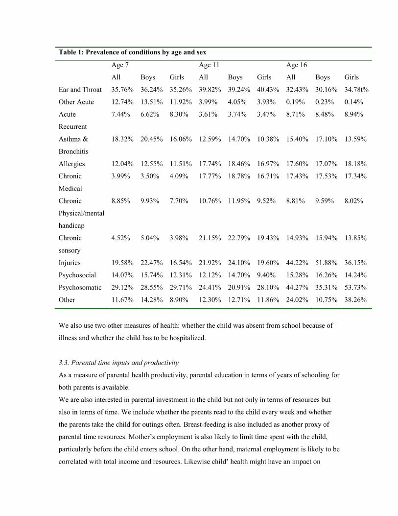
Table 1: Prevalence of conditions by age and sex

Age 7 Age 11 Age 16

All Boys Girls All Boys Girls All Boys Girls

Ear and Throat 35.76% 36.24% 35.26% 39.82% 39.24% 40.43% 32.43% 30.16% 34.78t%

Other Acute 12.74% 13.51% 11.92% 3.99% 4.05% 3.93% 0.19% 0.23% 0.14%

Acute

Recurrent

7.44% 6.62% 8.30% 3.61% 3.74% 3.47% 8.71% 8.48% 8.94%

Asthma &

Bronchitis

18.32% 20.45% 16.06% 12.59% 14.70% 10.38% 15.40% 17.10% 13.59%

Allergies 12.04% 12.55% 11.51% 17.74% 18.46% 16.97% 17.60% 17.07% 18.18%

Chronic

Medical

3.99% 3.50% 4.09% 17.77% 18.78% 16.71% 17.43% 17.53% 17.34%

Chronic

Physical/mental

handicap

8.85% 9.93% 7.70% 10.76% 11.95% 9.52% 8.81% 9.59% 8.02%

Chronic

sensory

4.52% 5.04% 3.98% 21.15% 22.79% 19.43% 14.93% 15.94% 13.85%

Injuries 19.58% 22.47% 16.54% 21.92% 24.10% 19.60% 44.22% 51.88% 36.15%

Psychosocial 14.07% 15.74% 12.31% 12.12% 14.70% 9.40% 15.28% 16.26% 14.24%

Psychosomatic 29.12% 28.55% 29.71% 24.41% 20.91% 28.10% 44.27% 35.31% 53.73%

Other 11.67% 14.28% 8.90% 12.30% 12.71% 11.86% 24.02% 10.75% 38.26%

We also use two other measures of health: whether the child was absent from school because of

illness and whether the child has to be hospitalized.

3.3. Parental time inputs and productivity

As a measure of parental health productivity, parental education in terms of years of schooling for

both parents is available.

We are also interested in parental investment in the child but not only in terms of resources but

also in terms of time. We include whether the parents read to the child every week and whether

the parents take the child for outings often. Breast-feeding is also included as another proxy of

parental time resources. Mother’s employment is also likely to limit time spent with the child,

particularly before the child enters school. On the other hand, maternal employment is likely to be

correlated with total income and resources. Likewise child’ health might have an impact on

maternal decision on whether to work or not and on mother’s labor supply.

Based on teacher’s assessment, there is some information on the level of interested of parents in

their child’s schooling. Another indication of investment is the information on parental wishes

about their offspring continuing their education.

In wave 3, parents report their cigarette consumption and this can also be a proxy of parental

attitudes towards health and health habits that can be transmitted.

3.4 Parental health

The NCDS records parental weight and height when the child is age 11. This information can be

transformed to obtain the Body mass Index (BMI) which is a measure of obesity. In addition,

chronic conditions for the father, mother and/or relatives is recorded in all waves during

childhood and adolescence. At age 7, the information is quite limited and it is only known

whether a relative had a congenital heart condition, diabetes or convulsions. At ages 11, the father

and the mother’s chronic condition is categorized according to the following groups:

Table 2: Parental chronic conditions

Age 11 Age 16

Mother Father Mother Father

Respiratory 12.55% 20.20% 14.86% 22.17%

Psychiatry 26.16% 11.94% 25.00% 10.06%

Subnormality 1.58% 0.20% 0.43%

Urogenital 9.28% 2.29% 3.43% 2.29%

Alimentary 6.33% 12.54% 5.57% 7.54%

Locomotory 11.71% 16.42% 11.57% 19.20%

Neurology 3.80% 5.17% 5.57% 4.91%

Infectious 0.84% 0.80% 1.14% 1.83%

Special 1.58% 2.495 3.57% 3.20%

Cardiovascular 14.56% 19.90% 12.14% 19.31%

Dermatological 1.58% 1.29% 1.43% 1.14%

Other 10.02% 6.77% 15.29% 8.34%

948 1005 700 875

Finally, when the cohort members are adults they are asked in wave 4 and 5 whether the father

and the mother are still alive.

3.5 Parental income

The information collected by the NCDS only contains one measure of family income when the

child is 16. This might not be a reflection of living standards earlier in childhood nor of persistent

poverty problems. For this reason, the data holders developed a measure of permanent income.

Using grouped dependent variable techniques and variables representing parental education,

occupation, age and region, they predicted permanent income. Because of the estimation

technique, this variable is therefore correlated with other variables of interest. In addition, there

are many missing cases because the following cases are excluded from the analysis: cases where

occupational class is missing and cases where the children are not living with either natural parent

at age 16.

We therefore experiment with several measures of income including whether the family had

serious financial difficulties, whether the child received free meals at school, and parental

socioeconomic status based on occupation.

3.6 Background characteristics

The dataset contains other additional information on the children’s background such as the sex,

number of siblings, birth order, region, and household composition, that is, whether the child had

one parental figure or not and which one (natural, adopted, foster, etc).

The NCDS includes a reduced number of children who have been adopted (around 200).

Adoption is assumed to be random and children are placed with the adoption family 3 months

after birth. This removes the potential bias that parents in better health select those children in

better health for adoption. The NCDS adoptees are illegitimate children who are randomly placed

for adoption. Because of this, we do have some information on both the birth mother and the

adoptive parents. Because of the nature of the data we have some information on the birth mother

and the adoptive parents, which is unusual and not often found in data.

3.7 Cohort member’s children

In addition, wave 5 includes information about the cohort members’ children. The sample

consists of 4207 children, of which 23 are adopted. This includes some information about the

pregnancy and the delivery (smoking, problems during labor, etc). The mother also reports

information on the child’s infectious illnesses (measles, chicken pox), hearing problems, speech

difficulties, as well as other conditions such as asthma, epilepsy, hay fever, eczema, migraine,

diabetes and behavioral problems. Two assessment tests are given to the children to evaluate their

reading and math abilities (Ppvt reading test and piat math test). They are nevertheless not the

same as those previously administered to the cohort members. There is only information at one

point in time for those children and it is done at a young age. In addition, there are issues of

selection since older children will be typically those from teenage mothers. The data would only

allow us to look at the correlation between parental illnesses and children’s illnesses but we won’t

be able to disentangle the genetic part and the environmental part. Because of the children’s age

we cannot look at variables such as years of education and labor market outcomes correlation

with the parents’.

4. Results

4.1 Prenatal factors and health at birth

Prenatal care shows to have a positive impact on the baby’s weight. Maternal smoking is

associated with lower birthweight. High socio-economic status or higher income appears to have

a positive impact on birthweight. Mother’s own physical characteristics such as height and weight

are as expected highly correlated with the baby’s own weight. Mother schooling appears to

increase birthweight only when gestation time is not taken into account. Problems during the

pregnancy such as bleeding and toxemia have a negative impact on health at birth. Obstetric

history also appears to matter as indicated by the negative effect pas stillbirths and a too short

interval between this birth and the previous one, while having more children increases the weight

of the subsequent children. Nevertheless these results do not take into account the potential

endogeneity of variables such as prenatal care choice, smoking, etc.

Table 3: Health at birth and maternal care

Estimated birthweight Log of estimated birthweight

number of prenatal

care visits

0.617 0.164 0.446 0.006 0.001 0.004

(19.46)** (5.48)** (11.34)** (20.27)** (4.57)** (11.59)**

Parity 1.331 1.100 1.180 0.011 0.009 0.010

(9.01)** (8.01)** (6.44)** (7.64)** (6.67)** (5.97)**

sex of child -4.658 -4.950 -4.931 -0.041 -0.044 -0.043

(14.66)** (17.08)** (12.67)** (12.71)** (15.75)** (12.32)**

mother's age -0.190 -0.047 -0.080 -0.002 -0.000 -0.001

(5.01)** (1.35) (1.70) (4.77)** (0.77) (1.62)

Mother smoking –

medium

-4.098 -3.330 -4.049 -0.038 -0.029 -0.035

(9.06)** (8.05)** (7.21)** (8.32)** (7.37)** (7.09)**

Mother smoking –

heavy

-6.150 -5.569 -6.220 -0.056 -0.050 -0.056

(12.20)** (12.08)** (9.91)** (11.08)** (11.13)** (9.93)**

high ses 1.467 1.257 0.014 0.011

(3.66)** (3.47)** (3.40)** (3.12)**

Permanent income 4.757 0.044

(4.14)** (4.28)**

Week of 1s mother

prenatal visit- 1st-

3rd

-13.198 -8.277 0.954 -0.162 -0.108 0.009

(4.17)** (2.91)** (0.23) (5.08)** (3.93)** (0.25)

Week of 1s mother

prenatal visit- 36

week

8.372 3.868 6.702 0.093 0.045 0.064

(3.75)** (1.78) (2.12)* (4.11)** (2.13)* (2.26)*

Mother’s weight

in stones >=15st

12.814 10.271 10.143 0.107 0.082 0.083

(5.54)** (4.69)** (3.46)** (4.60)** (3.86)** (3.17)**

Mother’s weight

in stones: under 7

-7.355 -6.749 -6.320 -0.075 -0.068 -0.058

(6.12)** (6.14)** (4.05)** (6.16)** (6.37)** (4.14)**

past stillbirths and

neonatal deaths

-4.267 -2.454 -1.758 -0.048 -0.028 -0.016

(7.03)** (4.42)** (2.28)* (7.93)** (5.14)** (2.32)*

Bleeding -2.250 -1.371 -0.382 -0.027 -0.017 -0.003

(6.28)** (4.21)** (0.86) (7.50)** (5.42)** (0.77)

Toxaemia -2.127 -1.839 -2.108 -0.023 -0.019 -0.021

(6.23)** (5.93)** (5.04)** (6.65)** (6.44)** (5.57)**

Interval between

births <=1 year

-4.730 -0.627 -2.058 -0.053 -0.010 -0.020

(4.39)** (0.61) (1.50) (4.89)** (0.98) (1.61)

Scotland 2.313 2.807 2.325 0.019 0.024 0.020

(3.87)** (5.12)** (3.20)** (3.11)** (4.46)** (3.05)**

Mother stayed in

school after

minimum age

1.333 0.470 0.687 0.015 0.006 0.007

(3.40)** (1.33) (1.42) (3.82)** (1.61) (1.67)

height of mum in

inches

0.776 0.826 0.787 0.006 0.007 0.007

(10.85)** (12.67)** (8.93)** (8.72)** (10.70)** (8.36)**

Gestationalperiod

in days

0.668 0.008 4.157

(62.12)** (73.36)** (58.08)**

Constant 75.256 -115.243 48.340 4.421 2.255 7497

(15.88)** (21.75)** (6.02)** (92.62)** (44.03)** 0.137

Observations 13797 12685 7497 13797 12685

R-squared 0.136 0.340 0.142 0.121 0.385

4.2 Child health and parental income

Our primary estimates for child health are presented in Table 4. Here we used the number of

chronic illnesses at 3 different ages (corresponding to the 3 waves) as a measure of health. We

also include another measure of health available at ages 11 and 16: whether the child was absent

from school due to illness. The estimates for chronic illnesses are obtained using OLS while those

for absence from school are obtained through a probit. We observe that the coefficient for the log

of permanent parental income is negative and significant for all measures except at age 7. The

size of the coefficient also increases with age, indicating that the income gradient becomes more

pronounced with age, which is in line with the results found by Case et al. (2002) using US data

but not with Currie et al. (2005) using British data. Compared to Case et al. (2002) our coefficient

for income is smaller at ages 7 and 11 while being larger at age 16. The inclusion of additional

controls such as family size and sex does not change primarily the results1.

1 We do not include additional controls such as the age of the parents, the absence of the father or mother, parental education, occupation or region because the permanent income was predicted using those variables. For all tables in

this section, we include only the relevant variables and/or those significant at least the 5% level.

Table 4: Health status and family income

Number of chronic illness School absences due to illness

Age 7 Age 11 Age 16 Age 11 Age 16

predicted

permanent

parental income

-0.119 -0.211 -0.493 -0.432 -1.169

(1.43) (2.26)* (5.02)** (5.90)** (11.34)**

Constant 2.388 3.170 5.056 1.866 4.580

(5.71)** (6.77)** (10.28)** (5.09)** (8.93)**

Observations 8478 8050 7757 8890 8890

R-squared 0.000 0.001 0.003

Controls for Sex and Family size

predicted

permanent

parental income

-0.155 -0.228 -0.436 -0.440 -1.060

(1.82) (2.39)* (4.41)** (5.88)** (10.09)**

Sex of child -0.182 -0.137 0.316 0.150 0.217

(5.87)** (3.93)** (7.12)** (5.52)** (5.94)**

Constant 2.905 3.501 4.237 1.679 3.540

(6.65)** (7.10)** (8.44)** (4.33)** (6.71)**

Observations 8466 8039 7743 8866 8870

R-squared 0.005 0.003 0.015

We account next for the possibility that our results may be due to heterogeneity of health

at birth. Indeed, as detailed by Case et al. (2002), children from a lower income family might be

born with worse health and might take longer to recover, partly explaining why income matters

for health at alter ages. We therefore include two indicators of health heterogeneity at birth. The

first one is the child’s birthweight and the second is an indicator of whether the child had an

illness in the first week after birth. The results (in Table 5) indicate that health at birth is an

important predictor of health during childhood and adolescence. Higher birthweight is associated

with a lower number of chronic illnesses at ages 7 and 11. At age 16, the coefficient is

insignificant, indicating that the effects of low birthweight might decrease with age. Birthweight

does not appear to matter for school illnesses. An illness at birth increases the number of chronic

illnesses at all ages. The coefficient does nevertheless decrease with age. We observe that the

effects of parental income slightly decrease with the inclusion of health at birth but that the

coefficient remains significant2. We include another specification with the interaction between

income and illness at birth in order to check whether poor birth health has larger adverse effects

for low income children. This term is negative but only significant for children at age 11.

Table 5: Health status and family income given health at birth

Number of chronic illness School absences due to

illness

Age 7 Age 11 Age 16 Age 11 Age 16

predicted permanent

parental income

-0.123 -0.204 -0.409 -0.442 -1.053

(1.44) (2.15)* (4.13)** (5.88)** (10.00)**

sex of child -0.188 -0.148 0.312 0.153 0.212

(6.01)** (4.19)** (8.50)** (5.58)** (5.74)**

Estimated

birthweight

-0.002 -0.003 -0.002 0.000 -0.001

(2.33)* (2.76)** (1.62) (0.42) (0.79)

Illness at birth 0.778 0.685 0.501 -0.012 -0.137

(8.37)** (6.63)** (4.66)** (0.15) (1.19)

Constant 2.964 3.685 4.283 1.645 3.608

(6.70)** (7.36)** (8.37)** (4.17)** (6.72)**

Observations 8435 8011 7715 8835 8840

R-squared 0.014 0.009 0.018

Poor birth at health and income interactions

predicted permanent

parental income

-0.107 -0.174 -0.386 -0.432 -1.037

2 We also observe that the decrease in the impact of income associated with the controls for health at birth is much lower than the one obtained by Case et al (2002) – where the coefficient becomes close to -0.09. In this sense, our results are more in line with Currie et al. (2004) who use British data.

(1.24) (1.81) (3.86)** (5.68)** (9.75)**

sex of child -0.187 -0.146 0.313 0.154 0.213

(5.98)** (4.14)** (8.53)** (5.60)** (5.75)**

Estimated

birthweight

-0.002 -0.003 -0.002 0.000 -0.001

(2.33)* (2.76)** (1.63) (0.42) (0.81)

Illness at birth 3.975 6.602 5.427 2.002 3.484

(1.51) (2.24)* (1.69) (0.84) (0.96)

Illness at

birth*family income

-0.641 -1.185 -0.987 -0.404 -0.733

(1.21) (2.01)* (1.53) (0.85) (1.00)

Constant 2.883 3.533 4.166 1.595 3.531

(6.45)** (6.98)** (8.05)** (4.00)** (6.51)**

Observations 8435 8011 7715 8835 8840

R-squared 0.014 0.010 0.018

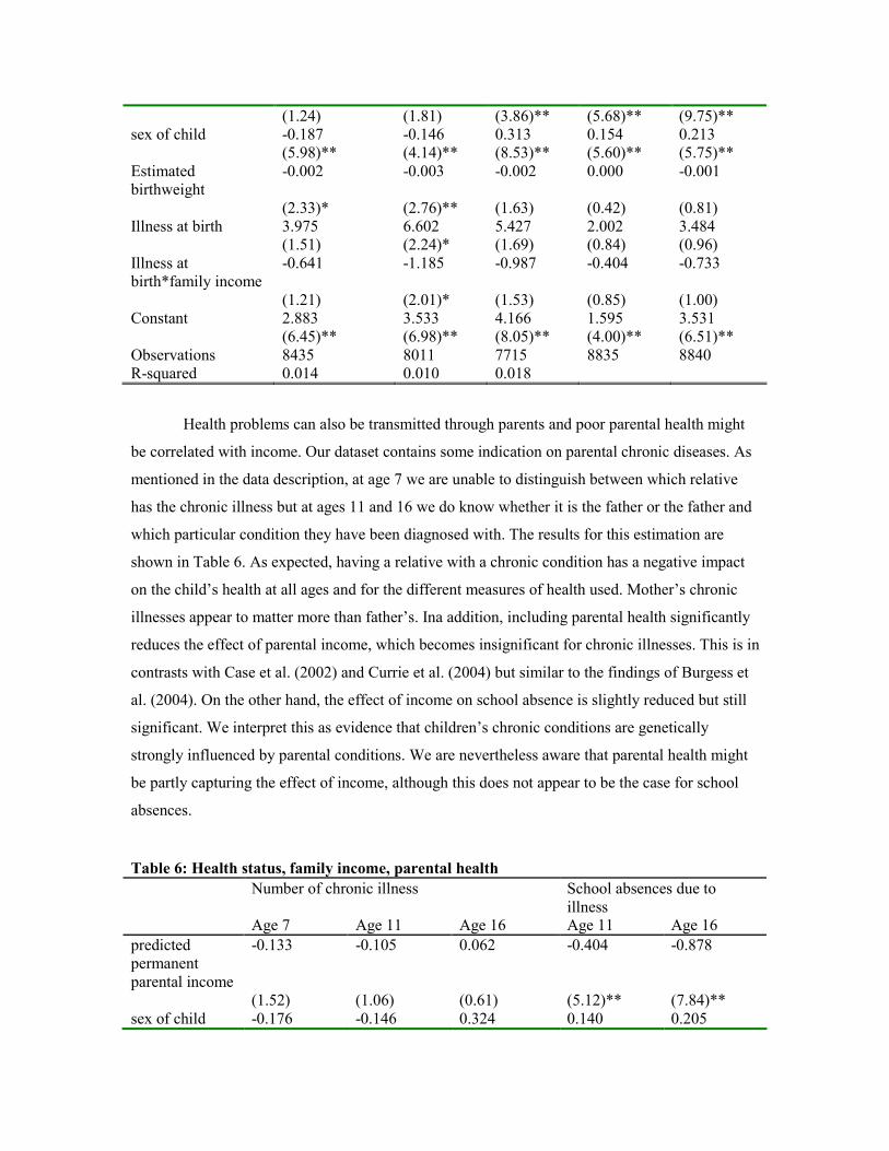
Health problems can also be transmitted through parents and poor parental health might

be correlated with income. Our dataset contains some indication on parental chronic diseases. As

mentioned in the data description, at age 7 we are unable to distinguish between which relative

has the chronic illness but at ages 11 and 16 we do know whether it is the father or the father and

which particular condition they have been diagnosed with. The results for this estimation are

shown in Table 6. As expected, having a relative with a chronic condition has a negative impact

on the child’s health at all ages and for the different measures of health used. Mother’s chronic

illnesses appear to matter more than father’s. Ina addition, including parental health significantly

reduces the effect of parental income, which becomes insignificant for chronic illnesses. This is in

contrasts with Case et al. (2002) and Currie et al. (2004) but similar to the findings of Burgess et

al. (2004). On the other hand, the effect of income on school absence is slightly reduced but still

significant. We interpret this as evidence that children’s chronic conditions are genetically

strongly influenced by parental conditions. We are nevertheless aware that parental health might

be partly capturing the effect of income, although this does not appear to be the case for school

absences.

Table 6: Health status, family income, parental health

Number of chronic illness School absences due to

illness Age 7 Age 11 Age 16 Age 11 Age 16

predicted

permanent

parental income

-0.133 -0.105 0.062 -0.404 -0.878

(1.52) (1.06) (0.61) (5.12)** (7.84)**

sex of child -0.176 -0.146 0.324 0.140 0.205

(5.57)** (4.09)** (9.02)** (5.00)** (5.39)**

Family illnesses 0.356

(7.27)**

Father chronic

illness

0.357 1.034 0.163 0.203

(4.95)** (15.09)** (2.91)** (3.14)**

Mother chronic

illness

0.577 1.327 0.208 0.323

(7.62)** (16.71)** (3.52)** (4.49)**

Bmi father -0.022 -0.019 -0.007 0.003 -0.003

(4.26)** (3.18)** (1.17) (0.59) (0.52)

Bmi mother 0.007 0.009 0.006 0.009 0.017

(1.77) (2.02)* (1.28) (2.53)* (3.74)**

Constant 3.141 3.124 1.597 1.245 2.268

(6.52)** (5.64)** (2.88)** (2.84)** (3.78)**

Observations 7963 7553 7262 8328 8320

R-squared 0.014 0.016 0.063

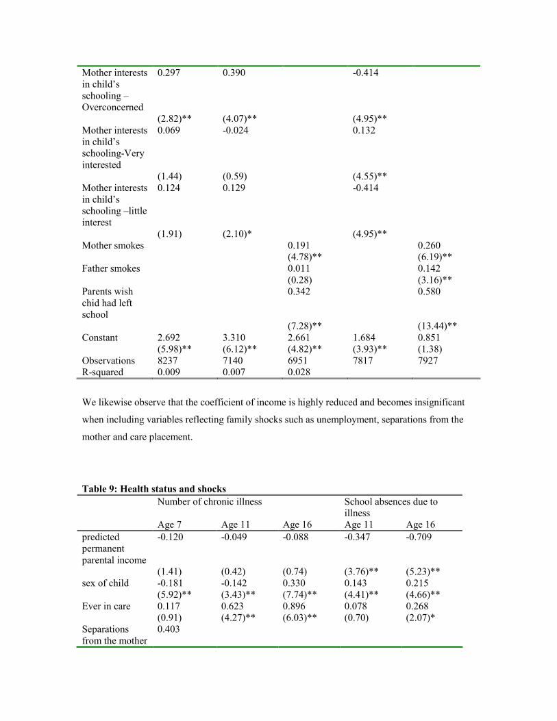
We are also interested in the effects of parental time and parental health behavior on

child’s health. We present the results on Table 7. We observe again that adding parental behavior

does reduce the impact of income on health and that the gradient disappears for the number of

chronic illnesses. Income does still matter for school absences due to illness. Father’s outing with

the child significantly reduces the number of chronic illnesses at age 7 but not at 11. Parental over

concern with schooling as assessed by the teacher appears to be positively correlated with the

number of chronic illnesses. Surprisingly children whose parents were over concerned with their

education and those whose parents showed little interest were less likely to miss school due to

illnesses. Parental wishes for lower education are associated with lower child’s health. Maternal

smoking is also significantly correlated with poor health.

Table 7: Health status, family income, parental behavior

Number of chronic illness School absences due to illness

Age 7 Age 11 Age 16 Age 11 Age 16

Predicted

permanent

parental income

-0.108 -0.187 -0.160 -0.414 -0.608

(1.21) (1.77) (1.49) (4.95)** (5.02)**

sex of child -0.191 -0.113 0.333 0.132 0.240

(6.10)** (3.06)** (8.74)** (4.55)** (5.89)**

Mother outings

with the child

0.090 -0.042 -0.414

(1.68) (0.67) (4.95)**

Father outings

with the child

-0.144 -0.083 0.132

(3.52)** (1.34) (4.55)**

Mother interests

in child’s

schooling –

Overconcerned

0.297 0.390 -0.414

(2.82)** (4.07)** (4.95)**

Mother interests

in child’s

schooling-Very

interested

0.069 -0.024 0.132

(1.44) (0.59) (4.55)**

Mother interests

in child’s

schooling –little

interest

0.124 0.129 -0.414

(1.91) (2.10)* (4.95)**

Mother smokes 0.191 0.260

(4.78)** (6.19)**

Father smokes 0.011 0.142

(0.28) (3.16)**

Parents wish

chid had left

school

0.342 0.580

(7.28)** (13.44)**

Constant 2.692 3.310 2.661 1.684 0.851

(5.98)** (6.12)** (4.82)** (3.93)** (1.38)

Observations 8237 7140 6951 7817 7927

R-squared 0.009 0.007 0.028

We likewise observe that the coefficient of income is highly reduced and becomes insignificant

when including variables reflecting family shocks such as unemployment, separations from the

mother and care placement.

Table 9: Health status and shocks

Number of chronic illness School absences due to

illness

Age 7 Age 11 Age 16 Age 11 Age 16

predicted

permanent

parental income

-0.120 -0.049 -0.088 -0.347 -0.709

(1.41) (0.42) (0.74) (3.76)** (5.23)**

sex of child -0.181 -0.142 0.330 0.143 0.215

(5.92)** (3.43)** (7.74)** (4.41)** (4.66)**

Ever in care 0.117 0.623 0.896 0.078 0.268

(0.91) (4.27)** (6.03)** (0.70) (2.07)*

Separations

from the mother

0.403

for more than a

week

(12.94)**

Domestic

problems

0.593

(7.85)**

Father

unemployed

0.022

(0.21)

Number of

Weeks dad off

work due to

illness

0.013 0.018 0.006 0.013

(4.71)** (6.05)** (3.06)** (5.21)**

Number of

Weeks dad off

work due to

unemployment

0.008 0.001 0.007 0.011

(2.06)* (0.26) (2.41)* (3.32)**

Number of

Weeks dad off

work due to

other causes

0.027 -0.002

(2.04)* (0.23)

Constant 2.579 2.608 2.378 1.251 1.676

(5.93)** (4.35)** (3.93)** (2.63)** (2.44)*

Observations 8425 5660 5498 6201 6223

R-squared 0.034 0.012 0.029

Finally, we compare different specifications for parental wealth: parental income, father’s

socioeconomic status (SES) at birth of the child and whether the family experienced financial

difficulties3. After inclusion of all the controls, neither parental income nor SES remain

significant. Financial difficulties however are significant at all ages and have a much higher

coefficient.

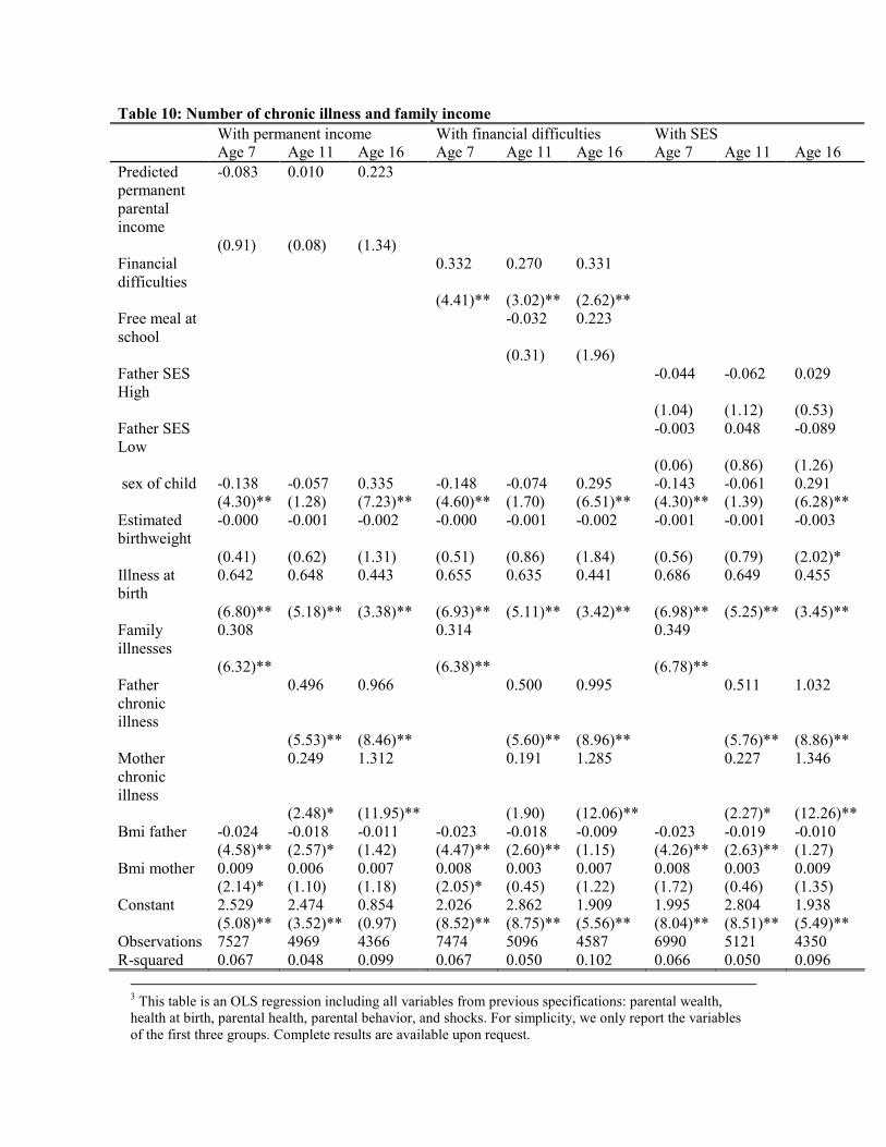
Table 10: Number of chronic illness and family income

With permanent income With financial difficulties With SES

Age 7 Age 11 Age 16 Age 7 Age 11 Age 16 Age 7 Age 11 Age 16

Predicted

permanent

parental

income

-0.083 0.010 0.223

(0.91) (0.08) (1.34)

Financial

difficulties

0.332 0.270 0.331

(4.41)** (3.02)** (2.62)**

Free meal at

school

-0.032 0.223

(0.31) (1.96)

Father SES

High

-0.044 -0.062 0.029

(1.04) (1.12) (0.53)

Father SES

Low

-0.003 0.048 -0.089

(0.06) (0.86) (1.26)

sex of child -0.138 -0.057 0.335 -0.148 -0.074 0.295 -0.143 -0.061 0.291

(4.30)** (1.28) (7.23)** (4.60)** (1.70) (6.51)** (4.30)** (1.39) (6.28)**

Estimated

birthweight

-0.000 -0.001 -0.002 -0.000 -0.001 -0.002 -0.001 -0.001 -0.003

(0.41) (0.62) (1.31) (0.51) (0.86) (1.84) (0.56) (0.79) (2.02)*

Illness at

birth

0.642 0.648 0.443 0.655 0.635 0.441 0.686 0.649 0.455

(6.80)** (5.18)** (3.38)** (6.93)** (5.11)** (3.42)** (6.98)** (5.25)** (3.45)**

Family

illnesses

0.308 0.314 0.349

(6.32)** (6.38)** (6.78)**

Father

chronic

illness

0.496 0.966 0.500 0.995 0.511 1.032

(5.53)** (8.46)** (5.60)** (8.96)** (5.76)** (8.86)**

Mother

chronic

illness

0.249 1.312 0.191 1.285 0.227 1.346

(2.48)* (11.95)** (1.90) (12.06)** (2.27)* (12.26)**

Bmi father -0.024 -0.018 -0.011 -0.023 -0.018 -0.009 -0.023 -0.019 -0.010

(4.58)** (2.57)* (1.42) (4.47)** (2.60)** (1.15) (4.26)** (2.63)** (1.27)

Bmi mother 0.009 0.006 0.007 0.008 0.003 0.007 0.008 0.003 0.009

(2.14)* (1.10) (1.18) (2.05)* (0.45) (1.22) (1.72) (0.46) (1.35)

Constant 2.529 2.474 0.854 2.026 2.862 1.909 1.995 2.804 1.938

(5.08)** (3.52)** (0.97) (8.52)** (8.75)** (5.56)** (8.04)** (8.51)** (5.49)**

Observations 7527 4969 4366 7474 5096 4587 6990 5121 4350

R-squared 0.067 0.048 0.099 0.067 0.050 0.102 0.066 0.050 0.096

3 This table is an OLS regression including all variables from previous specifications: parental wealth,

health at birth, parental health, parental behavior, and shocks. For simplicity, we only report the variables

of the first three groups. Complete results are available upon request.

4.3 Fixed-effects estimation

The effect of a change in financial difficulties since last wave appears to have an increase in the

number of chronic conditions. Comparing the size of the coefficient with the OLS estimation, the

panel data estimates are smaller. We also see that changes in the family composition matter for

the appearance of chronic conditions. Indeed, no longer being with one’s natural father raises the

number of chronic conditions.

Financial difficulties are instrumented by housing characteristics (house ownership, number of

rooms, availability of indoor lavatory and hot water). The results show that using instruments

highly increases the effects of financial difficulties on children’s health.

Table 11: Individual Fixed Effects Estimates for Health

Individual FE IV FE

Financial difficulties 0.157 0.169 0.176 0.159 3.188 (4.38)** (4.74)** (4.90)** (4.48)** (3.44)**

Number of children

in the household

-0.142 -0.144 -0.142 -0.179

(12.60)** (12.73)** (12.60)** (10.46)**

Non natural mother 0.310 0.294 0.262

(2.04)* (1.94) (1.48)

Non natural father 0.269 0.269 0.676

(3.06)** (3.07)** (4.19)**

Chronic illness in

the family

0.396 0.320

(14.16)** (8.00)**

Constant 2.096 2.518 2.508 2.453 2.287

(291.88)** (73.55)** (73.02)** (71.33)** (34.67)**

Observations 36275 36138 36136 36136 35979

R-squared 0.001 0.009 0.009 0.019

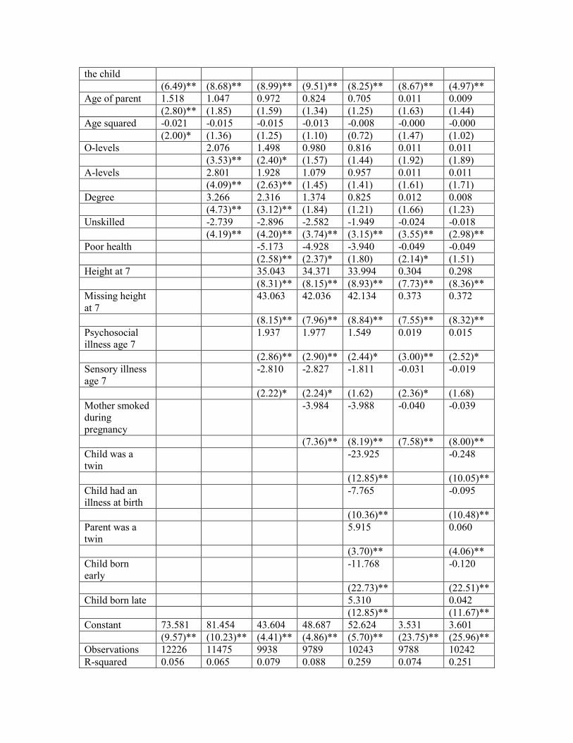
In the second stage, the fixed effects estimated from the first stage are regressed on covariates

representing parental health and behavior, and some individual characteristics. We observe that

individual effects are lower for females and for those with higher birthweight. Father’s year of

education is negative and significant while mother’s is positive. The opposite occurs with father’s

and mother’s Body mass Index. Children who suffered from illnesses at birth and the mother

experienced bleeding during the pregnancy have higher individual effects.

Table 12: Regressions on Fixed Effects

Variables FE model IV FE model

sex of child -0.043 -0.043 -0.045

(3.02)** (3.05)** (2.96)**

Parity 0.028 0.028 -0.023

(5.76)** (5.81)** (4.41)**

Bleeding during

pregnancy

0.147 0.148 0.160

(9.37)** (9.45)** (9.52)**

Toxemia -0.066 -0.066 -0.045

(4.52)** (4.52)** (2.88)**

Illness at birth 0.612 0.612 0.674

(14.85)** (14.87)** (15.23)**

Estimated birthweight -0.002 -0.002 -0.001

(5.32)** (5.37)** (1.49)

Bmi father -0.012 -0.012 -0.009

(5.00)** (5.05)** (3.27)**

Bmi mother 0.016 0.016 0.011

(8.30)** (8.35)** (5.57)**

Father’s years of

education

-0.019 -0.019 -0.001

(3.12)** (3.16)** (0.15)

Mother’s years of

education

0.020 0.019 0.037

(2.81)** (2.77)** (4.90)**

Family illnesses 0.422

(20.00)**

Breastfed 0.069 0.067 0.093

(4.53)** (4.46)** (5.72)**

Maternal smoking during

pregnancy

0.135 0.136 0.043

(8.92)** (9.03)** (2.67)**

bsag total score 0.014 0.014 0.006

(16.35)** (16.27)** (6.89)**

Constant -0.020 0.042 -0.314

(0.18) (0.38) (2.66)**

Observations 32102 32102 31973

R-squared 0.052 0.038 0.029

4.4 Cohort members and their children

Table 13: Regression of children’s Birthweight on parental birthweight and other parental

characteristics

With Birthweight With log of BW

Sex -10.238 -11.064 -11.493 -11.837 -7.169 -0.308 -0.172

(2.90)** (3.13)** (3.15)** (3.16)** (2.05)* (2.19)* (1.29)

Birthweight 0.148 0.140 0.122 0.124 0.123 0.145 0.141

(6.05)** (5.89)** (4.92)** (4.78)** (4.95)** (6.34)** (6.82)**

Sex*BW 0.099 0.105 0.108 0.106 0.075 0.066 0.040

(3.36)** (3.58)** (3.56)** (3.41)** (2.59)** (2.25)* (1.43)

Sex of the child -1.123 -1.380 -1.573 -1.460 -2.006 -0.011 -0.017

(2.68)** (3.22)** (3.43)** (3.19)** (4.78)** (2.48)* (4.05)**

Birth order of 1.717 2.375 2.687 2.920 2.394 0.025 0.018

the child

(6.49)** (8.68)** (8.99)** (9.51)** (8.25)** (8.67)** (4.97)**

Age of parent 1.518 1.047 0.972 0.824 0.705 0.011 0.009

(2.80)** (1.85) (1.59) (1.34) (1.25) (1.63) (1.44)

Age squared -0.021 -0.015 -0.015 -0.013 -0.008 -0.000 -0.000

(2.00)* (1.36) (1.25) (1.10) (0.72) (1.47) (1.02)

O-levels 2.076 1.498 0.980 0.816 0.011 0.011

(3.53)** (2.40)* (1.57) (1.44) (1.92) (1.89)

A-levels 2.801 1.928 1.079 0.957 0.011 0.011

(4.09)** (2.63)** (1.45) (1.41) (1.61) (1.71)

Degree 3.266 2.316 1.374 0.825 0.012 0.008

(4.73)** (3.12)** (1.84) (1.21) (1.66) (1.23)

Unskilled -2.739 -2.896 -2.582 -1.949 -0.024 -0.018

(4.19)** (4.20)** (3.74)** (3.15)** (3.55)** (2.98)**

Poor health -5.173 -4.928 -3.940 -0.049 -0.049

(2.58)** (2.37)* (1.80) (2.14)* (1.51)

Height at 7 35.043 34.371 33.994 0.304 0.298

(8.31)** (8.15)** (8.93)** (7.73)** (8.36)**

Missing height

at 7

43.063 42.036 42.134 0.373 0.372

(8.15)** (7.96)** (8.84)** (7.55)** (8.32)**

Psychosocial

illness age 7

1.937 1.977 1.549 0.019 0.015

(2.86)** (2.90)** (2.44)* (3.00)** (2.52)*

Sensory illness

age 7

-2.810 -2.827 -1.811 -0.031 -0.019

(2.22)* (2.24)* (1.62) (2.36)* (1.68)

Mother smoked

during

pregnancy

-3.984 -3.988 -0.040 -0.039

(7.36)** (8.19)** (7.58)** (8.00)**

Child was a

twin

-23.925 -0.248

(12.85)** (10.05)**

Child had an

illness at birth

-7.765 -0.095

(10.36)** (10.48)**

Parent was a

twin

5.915 0.060

(3.70)** (4.06)**

Child born

early

-11.768 -0.120

(22.73)** (22.51)**

Child born late 5.310 0.042

(12.85)** (11.67)**

Constant 73.581 81.454 43.604 48.687 52.624 3.531 3.601

(9.57)** (10.23)** (4.41)** (4.86)** (5.70)** (23.75)** (25.96)**

Observations 12226 11475 9938 9789 10243 9788 10242

R-squared 0.056 0.065 0.079 0.088 0.259 0.074 0.251

4.5 Children’s health by household composition

Table 13: Health status, family income, type

Number of chronic illness at age

7

Number of chronic illness at age

11

Number of chronic illness at age

16

Singletons Twins Adoptees Singletons Twins Adoptees Singletons Twins Adoptees

Estimated

birthweight

-0.003 -0.012 0.002 -0.004 -0.021 -0.000 -0.002 -0.009 0.005

(4.91)** (2.51)* (0.36) (4.42)** (3.20)** (0.00) (2.50)* (1.30) (0.58)

sex of child -0.242 0.035 -0.585 -0.198 -0.040 -0.410 0.278 0.199 -0.231

(9.67)** (0.21) (2.65)** (6.72)** (0.18) (1.48) (8.25)** (0.83) (0.75)

Constant 2.546 2.744 2.365 2.822 4.051 2.837 2.462 3.059 2.446

(26.82)** (5.04)** (2.96)** (25.27)** (5.60)** (2.68)** (19.06)** (3.98)** (2.20)*

Observations 13348 310 170 11415 254 134 9280 193 107

R-squared 0.008 0.021 0.042 0.005 0.039 0.017 0.009 0.014 0.010

References

Benzeval M, Judge K. Income and Health: The Time Dimension, Social Science and Medecine,

2001; 52: 1371-1390.

Burgess S, Propper C, Rigg J, the ALSPAC Study Team. The Impact of Low-Income on Child

Health: Evidence from a Birth Cohort Study, CMPO Working Paper Series, Working Paper

04/098, 2004.

Case A, Lubotsky M, Paxson C. Economic Status and Health in Childhood: The Origins of the

Gradient, American Economic Review, 2002; 92(5): 1308-1334.

Currie A, Shields MA, Wheatley Price S. Is the Child Health / Family Income Gradient

Universal? Evidence from England, IZA Discussion Paper Series, Discussion Paper No. 1328,

2004.

Currie J, Moretti E. Biology as Destiny? Short and Long-Run Determinants of Intergenerational

Transmission of Birth Weight, NBER Working Papers Series, Working Paper 11567, 2005.

Currie J, Stabile M. Socioeconomic Status and Child Health: Why Is the Relationship Stronger

for Older Children? American Economic Review 2003; 93(5): 1813-1823.

Davey Smith G, Hart C, Ferrell C, Upton M, Hole D, Hawthorne V, Watt G. Birth weight of

offspring and mortality in the Renfrew and Paisley study: prospective observational

study, British Medical Journal, 1997; 315: 1189-1193.

Doyle O, Harmon C, Walker I. The Impact of Parental Income and Education on the Health of

their Children, IZA Discussion Paper Series, Discussion Paper No. 1832, 2005.

Grossman M. On the concept of health capital and the demand for health. Journal of Political

Economy 1972; 80: 223-255.

Hyppönen E, Davey Smith G, Power C. Parental diabetes and birth weight of offspring:

intergenerational cohort study, British Medical Journal, 2003; 326: 19-20.

Kebede B. Genetic Endowments, Parental and Child Health in Rural Ethiopia. Scottish Journal of

Political Economy, 2005; 52(2): 194-221.

Power C, Peckham C. Childhood Morbidity and Adult Ill-Health, National child Development

Study User Support Group, Working Paper No. 37, 1987.

Rosenzweig MR, Schultz TP. Estimating a Household Production Function: Heterogeneity, the

Demand for Health Inputs, and Their Effect on Birth Weight, The Journal of Political Economy,

1983; 91(5): 723-746.

Rosenzweig MR, Wolpin KI. Heterogeneity, Intrafamily Distribution, and Child Health. The

Journal of Human Resources, 1988; 23(4): 437-461.

Appendix A

Table A1: Health information by generation

Generation1: Parents of the

cohort members

Generation 2: Cohort

members

Generation 3: children of the

cohort members

1) Before and/or during

pregnancy

a) Mother’s Height

b) Mother’s Weight

c) Prenatal care

d) Maternal smoking

e) Pregnancy-related

problems

(pleclampsia,

bleeding, toxemia and

low hemoglobin)

2) After pregnancy

a) Height and weight

b) Chronic conditions (in

wave 1- only 3

categories- and wave

2)

c) Date of death

d) Parental smoking

1) Health at birth

a) Birthweight (by

gestational age and

sex)

b) Illness in the first

week of life

2) During childhood

a) Accidents

b) Hospitalizations

c) Chronic conditions

(physical)

d) Acute conditions

e) Psychological

problems

3) In adulthood

a) SAH

b) Disability/LSI

c) Health behavior:

smoking, drinking,

exercise, nutrition

d) Height and weight

(self-reported)

1) Pregnancy information

2) Birthweight

3) Motor problems, chronic

conditions (asthma,

epilepsy, hay fever,

eczema, migraine,

diabetes), behavioral.